MorphoActivation: Generalizing ReLU activation function by mathematical morphology

Abstract

This paper analyses both nonlinear activation functions and spatial max-pooling for Deep Convolutional Neural Networks (DCNNs) by means of the algebraic basis of mathematical morphology. Additionally, a general family of activation functions is proposed by considering both max-pooling and nonlinear operators in the context of morphological representations. Experimental section validates the goodness of our approach on classical benchmarks for supervised learning by DCNN.

1 Introduction

Artificial neural networks were introduced as mathematical models for biological neural networks [24]. The basic component is a linear perceptron which is a linear combination of weights with biases followed by a nonlinear function called activation function. Such components (usually called a layer) can then be concatenated eventually leading to very complex functions named deep artificial neural networks (DNNs) [7]. Activation function can also be seen as an attached function between two layers in a neural network. Meanwhile, in order to get the learning in a DNNs, one needs to update the weights and biases of the neurons on the basis of the error at the output. This process involves two steps, a Back-Propagation from prediction error and a Gradient Descent Optimization to update parameters [7]. The most famous activation function is the Rectified Linear Unit (ReLU) proposed by [27], which is simply defined as $\texttt{ReLU}(x)=\max(x,0)$. A clear benefit of ReLU is that both the function itself and its derivatives are easy to implement and computationally inexpensive. However, ReLU has a potential loss during optimization because the gradient is zero when the unit is not active. This could lead to cases where there is a gradient-based optimization algorithm that will not adjust the weights of a unit that was never initially activated. An approach purely computational motivated to alleviate potential problems caused by the hard zero activation of ReLU, proposed a leaky ReLU activation [18]: $\texttt{LeakyReLU}(x)=\max(x,.01x)$. A simple generalisation is the Parametric ReLU proposed by [11], defined as $\texttt{PReLU}_{\beta}(x)=\max(x,\beta x)$, where $\beta\in\mathds{R}$ is a learnable parameter. In general, the use of piecewise-linear functions as activation function has been initially motivated by neurobiological observations; for instance, the inhibiting effect of the activity of a visual-receptor unit on the activity of the neighbouring units can be modelled by a line with two segments [10]. On the other hand, for the particular case of structured data as images, a translation invariant DNN called Deep Convolutional Neural Networks (DCNN) is the most used architecture. In the conventional DCNN framework interspersed convolutional layers and pooling layers to summarise information in a hierarchical structure. The common choice is the pooling by a maximum operator called max-pooling, which is particularly well suited to the separation of features that are very sparse [3].

As far as these authors know, that morphological operators have been used in the context of DCNNs following the paradigm of replacing lineal convolutions by non-linear morphological filters [31, 34, 15, 26, 13], or hybrid variants between linear and morphological layers [30, 32, 14, 33]. Our contribution is more in the sense of [5] where the authors show favourable results in quantitative performance for some applications when seeing the max-pooling operator as a dilation layer. However, we go further to study both nonlinear activation and max-pooling operators in the context of morphological representation theory of nonlinear operators. Finally, in the experimental section, we compare different propositions in a practical case of training a multilayer CNNs for classification of images in several databases.

2 ReLU activation and max-pooling are morphological dilations

2.1 Dilation and Erosion

Let us consider a complete lattice $({\cal L},\leq)$, where and $\bigvee$ and $\bigwedge$ are respectively its supremum and infimum. A lattice operator $\psi:{\cal L}\to{\cal L}$ is called increasing operator (or isotone) is if it is order-preserving, i.e., $\forall X,Y$, $X\leq Y\implies\psi(X)\leq\psi(Y)$. Dilation $\delta$ and erosion $\varepsilon$ are lattice operators which are increasing and satisfy

$$\delta\left(\bigvee_{i\in J}X_{i}\right)=\bigvee_{i\in J}\delta\left(X_{i}\right); \varepsilon\left(\bigwedge_{i\in J}X_{i}\right)=\bigwedge_{i\in J}\varepsilon\left(X_{i}\right).$$

Dilation and erosion can be then composed to obtain other operators [12]. In this paper, we also use morphological operators on the lattice of functions $\mathcal{F}(\mathds{R}^{n},\bar{\mathds{R}})$ with the standard partial order $\leq$. The sup-convolution and inf-convolution of function $f$ by structuring function $g$ are given by

$$(f\oplus g)(x)=\delta_{g}(f)(x) := \sup_{y\in\mathds{R}^{n}}\left\{f(x-y)+g(y)\right\},$$ (1)

$$(f\ominus g)(x)=\varepsilon_{g}(f)(x) := \inf_{y\in\mathds{R}^{n}}\left\{f(x+y)-g(y)\right\}.$$ (2)

2.2 ReLU and max-pooling

Let us now consider the standard framework of one-dimensional signals on DCNNs where any operator is applied on signals $f(x)$ supported on a discrete grid subset of $\mathbb{Z}$. The ReLU activation function [27] applied on every pixel $x$ of an image $f$ is defined as

$$\texttt{ReLU}(f(x)):=\max\left(0,f(x)\right).$$ (3)

The Max-pooling operator of pooling size $R$ and strides $K$, maps an image $f$ of $n$ pixels onto an image of $n^{\prime}:=\lfloor\frac{n-R}{K}+1\rfloor$ by taking the local maxima in a neighbour of size $R$, and moving the window $K$ elements at a time, skipping the intermediate locations:

$$\texttt{MaxPool}_{R}(f)(x)=\delta^{\texttt{MaxPool}}_{R}(f)(x):=\bigvee_{y\in W_{R}(x)}\{f(K\cdot x-y)\}.$$ (4)

where $W_{R}(y)=0$ if $y$ belongs to the neighbour of size $R$ centred in $x$ and $-\infty$ otherwise. There are other operations in DCNN which use the maximum operation as main ingredient, namely the Maxout layer [8] and the Max-plus layer (morphological perceptron) [4, 37].

From the definition of operators, it is straightforward to prove the following proposition

Proposition 1

ReLU activation function and max-pooling are dilation operators on the lattice of functions.

Proof

Using the standard partial ordering $\leq$, we note that both ReLU and max-pooling are increasing:

$$f\leq g\implies\texttt{ReLU}(f)\leq\texttt{ReLU}(g);\>\>\>\delta^{\texttt{MaxPool}}_{R}(f)\leq\delta^{\texttt{MaxPool}}_{R}(g).$$

They commute with supremum operation

$${\texttt{ReLU}}(f\vee g)={\texttt{ReLU}}(f)\vee{\texttt{ReLU}}(g);\>\>\>\delta^{\texttt{MaxPool}}_{R}(f\vee g)=\delta^{\texttt{MaxPool}}_{R}(f)\vee\delta^{\texttt{MaxPool}}_{R}(g).$$

These two operators are both also extensive, i.e., $f\leq\delta(f)$. ReLU is also idempotent, i.e., $\texttt{ReLU}(\texttt{ReLU}(f))=\texttt{ReLU}(f)$. Then ReLU is both a dilation and a closing.

Remark 1: Factoring activation function and pooling. The composition of dilations in the same complete lattice can often be factorized into a single operation. One can for instance define a nonlinear activation function and pooling dilation as

$$\delta^{\text{ActPool}}_{R;\alpha}(f)(x):=\bigvee_{y\in W_{R}(x)}\left\{\max\left(0,f(K\cdot x-y)+\alpha\right)\right\},$$

where $W$ denotes a local neighbour, usually a square of side $R$. Note that that analysis does not bring any new operator, just the interpretation of composed nonlinearities as a dilation.

Remark 2: Positive and negative activation function, symmetric pooling. More general ReLU-like activation functions also keep a negative part. Let us consider the two parameters $\beta^{+},\beta^{-}\in\mathds{R}$, we define $(\beta^{+},\beta^{-})$-ReLU as

$${\texttt{ReLU}}_{\beta^{+},\beta^{-}}(f)(x):=\left\{\begin{array}[]{ll}\beta^{+}f(x)&\text{if}\>\>\>f(x)>0\\ \beta^{-}f(x)&\text{if}\>\>\>f(x)\leq 0\end{array}\right.$$

In the case when $\beta^{+}\geq\beta^{-}$, one has

$${\texttt{ReLU}}_{\beta^{+},\beta^{-}}(f)(x)=\max\left(\beta^{-}f(x),\beta^{+}f(x)\right).$$ (5)

Note that the Leaky ReLU [18] corresponds to $\beta^{+}=1$ and $\beta^{-}=0.01$. The Parametric ReLU [11] takes $\beta^{+}=1$ and $\beta^{-}=\theta$ learned along with the other neural-network parameters. More recently [17] both $\beta^{+}$ and $\beta^{-}$ are learned in the ACtivateOrNot (ACON) activation function, where a softmax is used to approximate the maximum operator.

Usually in CNNs, the max-pooling operator is used after activation, i.e., $\delta^{\text{MaxPool}}_{R}({\texttt{ReLU}}_{\beta^{+},\beta^{-}}(f))$, which is spatially enlarging the positive activation and removing the negative activation. It does not seem coherent with the goal of using the pooling to increase spatial equivariance and hierarchical representation of information. It is easy to "fix" that issue by using a more symmetric pooling based on taking the positive and negative parts of a function. Given a function $f$, it can be expressed in terms of its positive $f^{+}$ and negative parts $f^{-}$, i.e., $f=f^{+}-f^{-}$, with $f^{+}(x)=\max(0,f(x))$ and $f^{-}(x)=\max(0,-f(x))$, where both $f^{+}$ and $f^{-}$ are non-negative functions. We can now define a positive and negative max-pooling. The principle is just to take a max-pooling to each part and recompose, i.e.,

$$\delta^{\texttt{MaxPool}^{+}_{-}}_{R}(f)(x) = \delta^{\texttt{MaxPool}}_{R}(f^{+})(x)-\delta^{\texttt{MaxPool}}_{R}(f^{-})(x)$$

$$= \delta^{\texttt{MaxPool}}_{R}(\max(0,f))(x)+\varepsilon^{\texttt{MinPool}}_{R}(\min(0,f))(x).$$

We note that (2.2) is self-dual and related to the dilation on an inf-semilattice [16]. However, in the general case of (2.2) by learning both $\beta^{-},\beta^{+}$,

$$\delta^{\texttt{MaxPool}^{+}_{-}}_{\beta^{+},\beta^{-},R}(f)(x)=\delta^{\texttt{MaxPool}}_{R}(\max(0,\beta^{-}f))(x)+\varepsilon^{\texttt{MinPool}}_{R}(\min(0,\beta^{+}f))(x)$$ (7)

is not always self-dual.

3 Algebraic theory of minimal representation for nonlinear operators and functions

In the following section, we present the main results about representation theory of nonlinear operators from Matheron [23], Maragos [20] and Bannon-Barrera [1] (MMBB).

3.1 MMBB representation theory on nonlinear operators

Let us consider a translation-invariant (TI) increasing operator $\Psi$. The domain of the functions considered here is either $E=\mathds{R}^{n}$ or $E=\mathbb{Z}^{n}$, with the additional condition that we consider only closed subsets of $E$. We consider first the set operator case applied on ${\cal P}(E)$ and functions $f:E\to\mathds{R}\cap\infty$.

Kernel and basis representation of TI increasing set operators. The kernel of the TI operator $\Psi$ is defined as the following collection of input sets [23]: $\text{Ker}(\Psi)=$ $\left\{A\subseteq E\>:\>\mathbf{0}\in\Psi(A)\right\}$, where $\mathbf{0}$ denotes the origin of $E$.

Theorem 3.1 (Matheron (1975) [23])

Consider set operators on ${\cal P}(E)$. Let $\Psi:{\cal P}(E)\to{\cal P}(E)$ be a TI increasing set operator. Then

$$\Psi(X)=\bigcup_{A\in\text{Ker}(\Psi)}X\ominus A=\bigcap_{B\in\text{Ker}(\bar{\Psi})}X\oplus\check{B}.$$

where the dual set operator is $\bar{\Psi}(X)=$ $[\Psi(X^{c})]^{c}$ and $\check{B}$ is the transpose structuring element.

The kernel of $\Psi$ is a partially ordered set under set inclusion which has an infinity number of elements. In practice, by the property of absorption of erosion, that means that the erosion by $B$ contains the erosions by any other kernel set larger than $B$ and it is the only one required when taking the supremum of erosions. The morphological basis of $\Psi$ is defined as the minimal kernel sets [20]:

$$\text{Bas}(\Psi)=\left\{M\in\text{Ker}(\Psi)\>:\>[A\in\text{Ker}(\Psi)\>\>\text{and}\>\>A\subseteq M]\implies A=M\right\}.$$

A sufficient condition for the existence of $\text{Bas}(\Psi)$ is for $\Psi$ to be an upper semi-continuous operator. We also consider closed sets on ${\cal P}(E)$.

Theorem 3.2 (Maragos (1989) [20])

Let $\Psi:{\cal P}(E)\to{\cal P}(E)$ be a TI, increasing and upper semi-continuous set operator . Then

$$\Psi(X)=\bigcup_{M\in\text{Bas}(\Psi)}X\ominus M=\bigcap_{N\in\text{Bas}(\bar{\Psi})}X\oplus\check{N}.$$

Kernel and basis representation of TI increasing operators on functions. Previous set theory was extended [20] to the case of mappings on functions $\Psi(f)$ and therefore useful for signal or grey-scale image operators. We focus on the case of closed functions $f$, i.e., its epigraph is a closed set. In that case, the dual operator is $\bar{\Psi}(f)=$ $-\Psi(-f)$ and the transpose function is $\check{f}(x)=$ $f(-x)$. Let

$$\text{Ker}(\Psi):=\left\{f\>:\Psi(f)(\mathbf{0})\geq 0\right\}$$

be the kernel of operator $\Psi$. As for the TI set operators, a basis can be obtained from the kernel functions as its minimal elements with respect to the partial order $\leq$, i.e.,

$$\text{Bas}(\Psi):=\left\{g\in\text{Ker}(\Psi)\>:\>[f\in\text{Ker}(\Psi)\>\>\text{and}\>\>f\leq g]\implies f=g\right\}.$$

This collection of functions can uniquely represent the operator.

Theorem 3.3 (Maragos (1989) [20])

Consider an upper semi-continuous operator $\Psi$ acting on an upper semi-continuous function $f$. Let $\text{Bas}(\Psi)=$ $\{g_{i}\}_{i\in I}$ be its basis and $\text{Bas}(\bar{\Psi})=$ $\{h_{j}\}_{j\in J}$ the basis of the dual operator. If $\Psi$ is a TI and increasing operator then it can be represented as

$$\Psi(f)(x) = \sup_{i\in I}\>(f\ominus g_{i})(x)=\sup_{i\in I}\>\inf_{y\in\mathbb{R}^{n}}\left\{f(x+y)-g_{i}(y)\right\}$$ (8)

$$= \inf_{j\in J}\>(f\oplus\check{h}_{j})(x)=\inf_{j\in J}\>\sup_{y\in\mathbb{R}^{n}}\left\{f(x-y)+\check{h}_{j}(y)\right\}$$ (9)

The converse is true. Given a collection of functions ${\cal B}=$ $\{g_{i}\}_{i\in I}$ such that all elements of it are minimal in $({\cal B},\leq)$, the operator $\Psi(f)=$ $\sup_{i\in I}$ $\{f\ominus g_{i}\}$ is a TI increasing operator whose basis is equal to ${\cal B}$.

For some operators, the basis can be very large (potentially infinity) and even if the above theorem represents exactly the operator by using a full expansion of all erosions, we can obtain an approximation based on smaller collections or truncated bases ${\cal B}\subset$ $\text{Bas}(\Psi)$ and $\bar{{\cal B}}\subset$ $\text{Bas}(\bar{\Psi})$. Then, from the operators $\Psi_{l}(f)=\sup_{g\in{\cal B}}\{f\ominus g\}$ and $\Psi_{u}(f)=\inf_{h\in\bar{{\cal B}}}\{f\oplus\check{h}\}$ the original $\Psi$ is bounded from below and above, i.e., $\Psi_{l}(f)\leq$ $\Psi(f)\leq$ $\Psi_{u}(f)$. Note also that in the case of a non minimal representation by a subset of the kernel functions larger than the basis, one just gets a redundant still satisfactory representation.

The extension to TI non necessarily increasing mappings was presented by Bannon and Barrera in [1], which involves a supremum of an operator involving an erosion and an anti-dilation. This part of the Matheron-Maragos-Bannon-Barrera (MMBB) theory is out of the scope of this paper.

3.2 Max-Min representation for Piecewise-linear functions

Let us also remind the fundamental results from the representation theory by Ovchinnikov [28, 29] which is rooted in a Boolean and lattice framework and therefore related to the MMBB theorems. Just note that here we focus on a representation for functions and previously it was a representation of operators on functions. Let $f$ be a smooth function on a closed domain $\Omega\subset\mathds{R}^{n}$. We are going to represent it by a family of affine linear functions $g_{t}$ which are tangent hyperplanes to the graph of $f$. Namely, for a point $t\in\Omega$, one defines

$$g_{t}(x)=\left\langle\nabla f(t),x-t\right\rangle+f(t),\>\>\>x\in\Omega,$$ (10)

where $\nabla f(t)$ is the gradient vector of $f$ at $t$. We have the following general result about the representation of piecewise-linear (PL) functions as max-min polynomial of its linear components.

Theorem 3.4 ([9][2][29])

Let $f$ be a PL function on a closed convex domain $\Omega\subset\mathds{R}^{n}$ and $\{g_{1}=\beta_{1}x+\alpha_{1},\cdots,g_{d}=\beta_{d}x+\alpha_{d}\}$ be the set of the $d$ linear components of $f$, with $\beta_{i},\alpha_{i}\in\mathds{R}^{n}$. There is a family $\{K_{i}\}_{i\in I}$ of subsets of set $\{1,\cdots,d\}$ such that

$$f(x)=\bigvee_{i\in I}\bigwedge_{j\in K_{i}}g_{j}(x),\>\>x\in\Omega.$$ (11)

Conversely, for any family of distinct linear functions $\{g_{1},\cdots,g_{d}\}$ the above formula defines a PL function.

The expression is called a max-min (or lattice) polynomial in the variable $g_{i}$. We note that a PL function $f$ on $\Omega$ is a “selector” of its components $g_{i}$, i.e., $\forall x\in\Omega$ there is an $i$ such that $f(x)=g_{i}(x)$. The converse is also true, with functions $\{g_{i}\}$ linearly ordered over $\Omega$ [29].

Let us also mention that from this representation we can show that a PL function is representable as a difference of two concave (equivalently, convex)-PL functions [29]. More precisely, let note $h_{i}(x)=\inf_{j\in K_{i}}g_{j}(x)$, with $h_{i}$ a concave function. We are reminded that sums and minimums of concave functions are concave. One have $h_{i}=$ $\sum_{k}h_{k}-\sum_{k\neq i}h_{k}$, therefore

$$f=\bigvee_{i\in I}h_{i}=\sum_{k}h_{k}-\bigwedge_{i\in I}\sum_{k\neq i}h_{k}.$$

4 Morphological universal activation functions

Using the previous results, we can state the two following results for the activation function and the pooling by increasing operators. Additionally, a proposed layer used in the experimental section is formulated.

4.1 Universal representation for activation function and pooling

Proposition 2

Any piecewise-linear activation function $\sigma:\mathds{R}\to\mathds{R}$ can be universally expressed as

$$\sigma(x)=\bigwedge_{j\in J}\left[\bigvee_{i\in I}\left\{\beta_{i}^{j}x+\alpha_{i}^{j}\right\}\right]=\bigwedge_{j\in J}p_{j}(x)$$ (12)

where $p_{j}=\bigvee_{i\in I}\left\{\beta_{i}^{j}x+\alpha_{i}^{j}\right\}$ is a PL convex function.

Proposition 3 (Pooling)

Any increasing pooling operator $\pi:\mathds{R}^{n}\to\mathds{R}^{n^{\prime}}$ can be universally expressed as

$$\pi(f)(x)=\bigwedge_{j\in J}\left[\delta_{b_{j}}(f)\right(K\cdot x)],$$ (13)

where $\{b_{j}\}_{j\in J}$ is a family of structuring functions defining by transpose the basis of the dual operator to $\pi$.

In both cases, there is of course a dual representation using the maximum of erosions. The dilation operator of type $z\mapsto\bigvee_{i}[\beta_{i}z+\alpha_{i}]$ plays a fundamental role in multiplicative morphology [12].

Remark: Tropical polynomial interpretation. The max-affine function $p_{j}=\bigvee_{i\in I}\left\{\beta_{i}^{j}z+\alpha_{i}^{j}\right\}$ is a tropical polynomial such that in that geometry, the degree of the polynomial corresponds to the number of pieces of the PL convex function. The set of such polynomials constitutes the semiring $\mathds{R}_{\max}$ of tropical polynomials. Tropical geometry in the context of lattice theory and neural networks is an active area of research [22] [21] [25], however those previous works have not considered the use of minimal representation of tropical polynomials as generalised activation functions.

Remark: Relationships to other universal approximation theorems. These results on universal representation of layers in DCNN are related to study the capacity of neural networks to be universal approximators for smooth functions. For instance, both maxout networks [8] and max-plus networks [37] can approximate arbitrarily well any continuous function on a compact domain. The proofs are based on the fact that [35] continuous PL functions can be expressed as a difference of two convex PL functions, and each convex PL can be seen as the maximum of affine terms.

Tropical formulation of ReLU networks has shown that a deeper network is exponentially more expressive than a shallow network [36]. To explore the expressiveness of networks with our universal activation function and pooling layer respect to the deepness of DCNN is therefore a fundamental relevant topic for future research.

4.2 MorphoActivation Layer

We have now all the elements to justify why in terms of universal representation theory of nonlinear operators ReLU and max-pooling can be replaced by a more general nonlinear operator defined by a morphological combination of activation function, dilations and downsampling, using a max-plus layer or its dual.

More precisely, we introduce two alternative architectures of the MorphoActivation layer (Activation and Pooling Morphological Operator) $f\mapsto$ $\Psi^{\text{Morpho}}:\mathds{R}^{n}\to\mathds{R}^{n^{\prime}}$ either by composition $[\pi\circ\sigma(f)](x)$ or $[\sigma\circ\pi(f)](x)$ as follows:

$$\Psi^{\text{Morpho}}_{1}(f)=\bigwedge_{1\leq j\leq M}\left\{\delta^{\texttt{MaxPool}}_{R,b_{j}}\left(\bigvee_{1\leq i\leq N}(\beta_{i}^{j}f+\alpha_{i}^{j})\right)\right\},$$ (14)

$$\Psi^{\text{Morpho}}_{2}(f)=\bigwedge_{1\leq i\leq N}\left\{\bigvee_{1\leq j\leq M}\left(\beta_{i}^{j}\delta^{\texttt{MaxPool}}_{R,b_{i}}(f)+\alpha_{i}^{j}\right)\right\},$$ (15)

where

$$\left\{\begin{array}[]{l}\delta^{\texttt{MaxPool}}_{R,b_{j}}(f)(x)=\delta_{b_{j}}(f)(R\cdot x),\>\>\>\>\text{with}\\ \\ \delta_{b_{j}}(f)(x)=(f\oplus b_{j})(x)=\bigvee_{y\in W}\{f(x-y)+b_{j}(y)\}\end{array}\right.$$

In the context of an end-to-end learning DCNN, the parameters $\beta_{j}$, $\alpha_{j}$ and structuring functions $b_{j}$ are learnt by backpropagation [34]. The learnable structuring functions $\mathbf{b}_{j}$ play the same role as the kernel in the convolutions. Note that one can have $R=1$, the pooling does not involve downsampling. We note that in a DCNN network the output of each layer $T^{k}$ is composed of the affine function $x\mapsto\mathbf{W}^{k}x+\mathbf{b}^{k}$, where $\mathbf{W}^{k}$ is the weight matrix (convolution weights in a CNN layer) and $\mathbf{b}^{k}$ the bias, and the activation function $\sigma$, i.e., $T^{k}=$ $\sigma\left(\mathbf{W}^{k}T^{k-1}+\mathbf{b}^{k}\right)$, where $\sigma$ is acting elementwise. Using our general activation (12), we obtain that

$$T^{k}=\bigwedge_{j\in J}\left[\bigvee_{i\in I}\left\{\beta_{i}^{jk}\mathbf{W}^{k}T^{k-1}+\beta_{i}^{jk}\mathbf{b}^{k}+\alpha_{i}^{jk}\right\}\right],$$

and therefore the bias has two terms which are learnt. We propose therefore to consider in our experiments that $\mathbf{b}^{k}$ is set to zero since its role will be replaced by learning the $\alpha_{i}^{jk}$.

5 Experimental Section

Firstly, to illustrate the kind of activation functions that our proposition can learn, we use the MNIST dataset as a ten class supervised classification problem and an architecture composed of two convolutional layers and a dense layer for reducing to the number of classes. The activation functions that we optimise by stochastic gradient descent have as general form $\min(\max(\beta_{0}x+\alpha_{0},\beta_{1}x+\alpha_{1},\alpha_{2}),\alpha_{3})$, which corresponds to (14) and (15) where $R=1$, i.e., without pooling. We have initialised all the activation functions to be equal to $\max(\min(\texttt{ReLU}(x),6),-6)$ as it is illustrated in Fig.1(left). The accuracy of this network without any training is $14\%$. Surprisingly when one optimises only the parameters of activation functions the network accuracy increases to the acceptable performance of $92.38\%$ and a large variability of activation functions are found Fig.1(center). This is a way to assess the expressive power of the parameter of the activation as it has been proposed in [6]. Additionally, an adequate separation among classes is noted by visualising the projection to two-dimensional space of the last layer via the t-SNE [19] algorithm. Of course, a much better accuracy ($98,58\%$) and inter-class separation is obtained by optimising all the parameters of the network Fig.1(right).

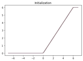
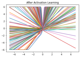
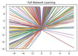
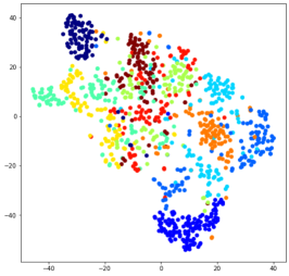
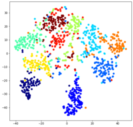
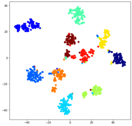
Figure 1: First Row: Left: Random Initialisation with (14%) of accuracy on the test set, We use a simplified version of proposed activation $\min(\max(\beta_{0}x+\alpha_{0},\beta_{1}x+\alpha_{1},\alpha_{2}),\alpha_{3})$, with initialisation $\max(\min(\texttt{ReLU}(x),6),-6)$ Centre: Training only activation functions (92.38%), Right: Training Full Network (98,58%). Second Row: t-SNE visualisation of last layer is the 10-classes MNIST prediction for a CNN.

Secondly, we compare the performance of (2.2), (7), (14) and (15) following the common practice and train all the models using a training set and report the standard top-one error rate on a testing set. We use as architecture a classical two-layer CNN (without bias for (14) and (15)) with 128 filters of size ($3\times 3$) per layer, and a final dense layer with dropout. After each convolution the different propositions are used to both produce a nonlinear mapping and reduce spatial dimension via pooling stride of two. As a manner of comparison, we include the case of a simple ReLU activation followed by a MaxPool with stride two. The difference in top-one error rate on a testing set is reported in Table 1 for CIFAR10, CIFAR100 and Fashion-MNIST databases. These quantitative results shown in propositions (2.2) and (7) do not seem to improve the performance in the explored cases. Additionally, (15) performs better than (14), and it improves the accuracy in comparison with our baseline in all the considered databases.

	Fashion MNIST			CIFAR10			CIFAR100
MaxPool(ReLU)	93.11			78.04			47.57
Self-dual Relu in (2.2)	-2.11			-20.12			-31.14
(7)	-0.95			-1.75			-4.39
MorphoActivation in (14)	N=2	N=3	N=4	N=2	N=3	N=4	N=2	N=3	N=4
M=2	-0.06	-0.05	-0.1	-0.42	0.02	-0.02	0.44	0.7	0.4
M=3	-0.14	-0.14	-0.06	-0.57	-0.4	-0.35	0.56	0.49	0.61
M=4	-0.02	-0.08	-0.01	0.05	-0.62	-0.5	0.41	0.35	0.73
MorphoActivation in (15)	N=2	N=3	N=4	N=2	N=3	N=4	N=2	N=3	N=4
M=2	0.04	-0.16	-0.12	1.84	2.02	1.49	3.31	3.5	3.45
M=3	0.08	-0.09	0.12	2.39	1.96	1.82	3.48	3.55	3.86
M=4	-0.02	0.09	-0.03	2.49	2.25	2.13	3.47	3.73	3.58

Table 1: Relative difference with respect to our baseline (ReLU followed by a MaxPool). Architecture used is a CNN with two layers. ADAM optimiser with an early stopping with patience of ten iterations. Only Random Horizontal Flip has been used as image augmentation technique for CIFARs. The results are the average over three repetitions of the experiments.

6 Conclusions and Perspectives

To the best of our knowledge, this is the first work where nonlinear activation functions in deep learning are formulated and learnt as max-plus affine functions or tropical polynomials. We have also introduced an algebraic framework inspired from mathematical morphology which provides a general representation to integrate the nonlinear activation and pooling functions.

Besides more extended experiments on the performance on advanced DCNN networks, our next step will be to study the expressivity power of the networks based on our morphological activation functions. The universal approximation theorems for ReLU networks would just be a particular case. We conjecture that the number of parameters we are adding on the morphological activation can provide a benefit to get more efficient approximations of any function with the same width and depth.

Acknowledgements

This work has been supported by Fondation Mathématique Jacques Hadamard (FMJH) under the PGMO-IRSDI 2019 program. This work was granted access to the Jean Zay supercomputer under the allocation 2021-AD011012212R1.

References

- [1] Banon, G.J.F., Barrera, J.: Minimal representations for translation-invariant set mappings by mathematical morphology. SIAM Journal on Applied Mathematics 51(6), 1782–1798 (1991)
- [2] Bartels, S.G., Kuntz, L., Scholtes, S.: Continuous selections of linear functions and nonsmooth critical point theory. Nonlinear Analysis: Theory, Methods & Applications 24(3), 385–407 (1995)
- [3] Boureau, Y.L., Ponce, J., LeCun, Y.: A theoretical analysis of feature pooling in visual recognition. In: ICML. pp. 111–118 (2010)
- [4] Charisopoulos, V., Maragos, P.: Morphological perceptrons: geometry and training algorithms. In: ISMM. pp. 3–15. Springer (2017)
- [5] Franchi, G., Fehri, A., Yao, A.: Deep morphological networks. Pattern Recognition 102, 107246 (2020)
- [6] Frankle, J., Schwab, D.J., Morcos, A.S.: Training batchnorm and only batchnorm: On the expressive power of random features in cnns. ICLR (2021)
- [7] Goodfellow, I., Bengio, Y., Courville, A.: Deep learning. MIT press (2016)
- [8] Goodfellow, I., Warde-Farley, D., Mirza, M., Courville, A., Bengio, Y.: Maxout networks. In: ICML. pp. 1319–1327 (2013)
- [9] Gorokhovik, V.V., Zorko, O.I., Birkhoff, G.: Piecewise affine functions and polyhedral sets. Optimization 31(3), 209–221 (1994)
- [10] Hartline, H.K., Ratliff, F.: Inhibitory interaction of receptor units in the eye of limulus. The Journal of General Physiology 40(3), 357–376 (1957)
- [11] He, K., Zhang, X., Ren, S., Sun, J.: Delving deep into rectifiers: Surpassing human-level performance on imagenet classification. In: IEEE ICCV. pp. 1026–1034 (2015)
- [12] Heijmans, H.J.A.M.: Theoretical aspects of gray-level morphology. IEEE Transactions on Pattern Analysis & Machine Intelligence 13(06), 568–582 (1991)
- [13] Hermary, R., Tochon, G., Puybareau, É., Kirszenberg, A., Angulo, J.: Learning grayscale mathematical morphology with smooth morphological layers. Journal of Mathematical Imaging and Vision (2022)
- [14] Hernández, G., Zamora, E., Sossa, H., Téllez, G., Furlán, F.: Hybrid neural networks for big data classification. Neurocomputing 390, 327–340 (2020)
- [15] Islam, M.A., Murray, B., Buck, A., Anderson, D.T., Scott, G.J., Popescu, M., Keller, J.: Extending the morphological hit-or-miss transform to deep neural networks. IEEE Transactions on NNs and Learning Systems 32(11), 4826–4838 (2020)
- [16] Keshet, R.: Mathematical morphology on complete semilattices and its applications to image processing. Fundamenta Informaticae 41(1-2), 33–56 (2000)
- [17] Ma, N., Zhang, X., Liu, M., Sun, J.: Activate or not: Learning customized activation. In: IEEE CVPR. pp. 8032–8042 (2021)
- [18] Maas, A.L., Hannun, A.Y., Ng, A.Y., et al.: Rectifier nonlinearities improve neural network acoustic models. In: Proc. ICML. vol. 30, p. 3 (2013)
- [19] Van der Maaten, L., Hinton, G.: Visualizing data using t-SNE. Journal of Machine Learning Research 9(11) (2008)
- [20] Maragos, P.: A representation theory for morphological image and signal processing. IEEE Tran. on Pattern Analysis and Machine Intel. 11(6), 586–599 (1989)
- [21] Maragos, P., Charisopoulos, V., Theodosis, E.: Tropical geometry and machine learning. Proceedings of the IEEE 109(5), 728–755 (2021)
- [22] Maragos, P., Theodosis, E.: Multivariate tropical regression and piecewise-linear surface fitting. In: ICASSP. pp. 3822–3826. IEEE (2020)
- [23] Matheron, G.: Random sets and integral geometry. John Wiley & Sons (1974)
- [24] McCulloch, W.S., Pitts, W.: A logical calculus of the ideas immanent in nervous activity. The Bulletin of Mathematical Biophysics 5(4), 115–133 (1943)
- [25] Misiakos, P., Smyrnis, G., Retsinas, G., Maragos, P.: Neural network approximation based on hausdorff distance of tropical zonotopes. In: ICLR. pp. 0–8 (2022)
- [26] Mondal, R., Dey, M.S., Chanda, B.: Image restoration by learning morphological opening-closing network. MM-Theory and Applications 4(1), 87–107 (2020)
- [27] Nair, V., Hinton, G.E.: Rectified linear units improve restricted boltzmann machines. In: ICML (2010)
- [28] Ovchinnikov, S.: Boolean representation of manifolds functions. J. Math. Anal. Appl. 263, 294–300 (2001)
- [29] Ovchinnikov, S.: Max–min representations of piecewise linear functions. Beiträge Algebra Geom. 43, 297–302 (2002)
- [30] Pessoa, L.F., Maragos, P.: Neural networks with hybrid morphological/rank/linear nodes: a unifying framework with applications to handwritten character recognition. Pattern Recognition 33(6), 945–960 (2000)
- [31] Ritter, G.X., Sussner, P.: An introduction to morphological neural networks. In: 13th International Conf. on Pattern Recognition. vol. 4, pp. 709–717. IEEE (1996)
- [32] Sussner, P., Campiotti, I.: Extreme learning machine for a new hybrid morphological/linear perceptron. Neural Networks 123, 288–298 (2020)
- [33] Valle, M.E.: Reduced dilation-erosion perceptron for binary classification. Mathematics 8(4), 512 (2020)
- [34] Velasco-Forero, S., Pagès, R., Angulo, J.: Learnable EMD based on mathematical morphology. SIAM Journal on Imaging Sciences 15(1), 23–44 (2022)
- [35] Wang, S.: General constructive representations for continuous piecewise-linear functions. IEEE Trans. on Circuits and Systems I 51(9), 1889–1896 (2004)
- [36] Zhang, L., Naitzat, G., Lim, L.H.: Tropical geometry of deep neural networks. In: International Conference on Machine Learning. pp. 5824–5832. PMLR (2018)
- [37] Zhang, Y., Blusseau, S., Velasco-Forero, S., Bloch, I., Angulo, J.: Max-plus operators applied to filter selection and model pruning in NNs. In: ISMM. pp. 310–322 (2019)