River Surface Patch-wise Detector Using Mixture Augmentation for Scum-cover-index

Abstract

Urban rivers provide a water environment that influences residential living. River surface monitoring has become crucial for making decisions about where to prioritize cleaning and when to automatically start the cleaning treatment. We focus on the organic mud, or “scum”, that accumulates on the river’s surface and contributes to the river’s odor and has external economic effects on the landscape. Because of its feature of a sparsely distributed and unstable pattern of organic shape, automating the monitoring process has proved difficult. We propose a patch-wise classification pipeline to detect scum features on the river surface using mixture image augmentation to increase the diversity between the scum floating on the river and the entangled background on the river surface reflected by nearby structures like buildings, bridges, poles, and barriers. Furthermore, we propose a scum-index cover on rivers to help monitor worse grade online, collect floating scum, and decide on chemical treatment policies. Finally, we demonstrate the application of our method on a time series dataset with frames every ten minutes recording river scum events over several days. We discuss the significance of our pipeline and its experimental findings.

River surface detection, Image augmentation, Patch-wise monitoring, Scum-cover-ratio, Scaled heatmap.

1 Introduction

1.1 Related Works

Automated garbage collection and river cleaning robots have been the center of river manager assisted robotics research for the past decade [1,2]. Additionally, river surface monitoring has become crucial to decide which areas are the worst and to automatically begin the cleaning process. Since 1991, there have been numerous studies for understanding the scum formation mechanism, such as in-house experiments [3,4], field observations regarding organic sludge and odor [5,6], and automatic scum behavior monitoring using river surface computer vision [7,8]. Owing to the complex events and intertwined phenomena that include physical, chemical, biological, and hydrological features, it is not widely known how to fundamentally solve the river scum problem.

After a few days of rainfall, combined sewer overflows (CSOs) suddenly occur at the upstream of the river owing to scum and the highly dispersed residential living environment. This organic mud or “scum” that appears on the river’s surface contributes to the river’s odor and has external economic effects on the landscape. Mizuta et al. [8] proposed a method for monitoring scum in an urban river’s tidal area. The 805 split lattice color images with a 20 $\times$ 20 pixel size were automatically used by the fixed point camera to determine whether or not scum was present. The accuracy for identifying the scum ranged from 58 to 88 percent using this straightforward neural network model with one hidden layer. The input variables included the 45 features of statistics and 25, 50, and 75 percentiles for each pixel’s RGB components. Additionally, they included input features like bridges and fences as reflected background features that were visible on the water surface. Although this was a preliminary version of the scum monitoring method, there is still room for accuracy enhancement and generalization to deep learning algorithms for pixel-by-pixel classification, also known as semantic segmentation, such as the U-Net [9]. Nakatani et al. [10] studied detailed observations of scum using multiple cameras and sediment surveys in a tidal river to understand the generation and floating behavior of scum using the U-Net. They discovered evidence that the local flow may have a significant impact on the spatial-temporal behavior of the scum owing to the tide level. Semantic segmentation is unquestionably a possible option for a rough scum monitoring method. If we use the marine debris object type [11,12], which includes bottles, cans, hooks, and tires, the U-Net with the ResNet34 backbone was still the best performing model. However, it has not always scored high accuracy with a mean Intersection of Union, 0.748.

However, the scum feature has a sparsely distributed and unstable pattern, which makes it difficult to improve the semantic segmentation accuracy. The scum segmentation on the river surface still has an over-prediction issue, and is insufficiently accurate for scum monitoring on the river water surface. The area of interest, the scum, was obscured by the water surface, which frequently reflected the nearby background features such as the building, bridge, pole, sign, sky, and trees. The authors propose a patch-wise classification method using image augmentation to improve the precise recognition of the river scum.

1.2 Pixel-wise Segmentation vs Patch Classification

First, we debate whether supervised learning such as that used in classification, object detection, and semantic segmentation, is a better deep learning approach. We can select semantic segmentation or classification if the target feature of the scum is not categorized into object context. It becomes challenging to annotate the scum feature on the pixel-wise region of interest (ROI) within the river surface in the case of the semantic segmentation. The scum features are sparsely dispersed, and the pattern is unstable and complex If we attempt to annotate one of the filled regions with multiple scum features, the trained learners would be low precision and the false negative error would increase resulting in a prediction of scum when it is actually background. Therefore, the authors proposed a patch-wise classification approach rather than the pixel-wise semantic segmentation. The patch size is 128 $\times$ 256. In contrast, we can consider an approach from unsupervised learning like the generator and anomaly detection such as the Variational Auto-Encoder (VAE) [13].

Figure 1: Scum Feature of z-space Trained from Three Classes Conditional VAE (defined by C0:early scum, C1:grow-thick scum, C2:background. Training dataset has respectively (5,026, 4,070, 4,308). Test dataset has each classes (550, 450, 470).)

As illustrated in Fig.1, we demonstrated how to train the three classes of conditional VAE [14] using a dataset that was defined by C0. “early scum,” C1. “grow-thick scum,” and C2. “background.” Here, the bridge z-space contains 256 elements. Using t-SNE, we could dimension-reduce the z-mean and z-variance into plots of two and three dimensions. Hence, the three classes of river water surface, scum-generated feature, and a background that includes the building, train, bridge, barrier, pole, and tree, were not independent of each other. Here, a fake scene was reflected on the river’s water surface with a mirrored background rather than an actual image. River water surface images are very complex and are dependent on the water surface class and the target scum feature. Therefore, we did not select the generative learning and pixel-wise segmentation approaches. We discovered that it did not fit the dataset of river scum images for accurate scum detection. To tackle the low precision problem, this study proposed a patch-wise classification approach using mixture image augmentation.

Figure 2: Pipeline Overview from a Camera Frame Input to Scum-cover-index

1.3 Overview of Pipeline

As shown in Fig.2, we give an overview of the pipeline from the offline training stage to the online prediction and computing scum index. The first three components of the training stage are 1) data preparedness, 2) mixture image augmentation, 3) patch-classification deep learning. The data preparation process involves cropping a rectangle without the far region’s top and extracting four rows by five columns of patch images. Mixture image augmentation [15] transforms into diversified images using multiple raw images, such as the mixup [16,17], Cutout [18], and random image cropping and patching (RICAP) [19]. Convolutional neural networks (CNNs), such as ResNet50, ResNet101, and Inception-v3, are used in deep learning for patch classification. Second, the prediction stage using the pretrained deep network includes the following steps: 1) predict 20 patch probabilities; 2) combine their probabilities into a matrix; 3) create a scaled heatmap; 4) binarize the mask image; and 5) calculate the pixel count of the scum region. The prediction brings the total number of patch probabilities taken from the raw input frame to 20. Their probability values are combined into a matrix. The matrix with four rows by five columns is transformed into a scaled heatmap with a grayscale intensity range of 0 to 255. The heatmap can binarize a mask image with pixels set to 0 or 1. The scum region pixel with a value of one on the mask image can be counted. Finally, the temporal scum index at a time stamp is computed as the value we call “scum-cover-ratio” whose scum region pixel count is divided by the river region pixel count, ranging from 0 to 100 percent. Here, the river region can count pixels without a background. The background region is constant when the camera angle is fixed, allowing us to set the river region’s pixel count. We can repeatedly calculate the scum-cover-ratio using the raw input frame image collected every ten minutes. We can visualize the time series of scum-cover-ratio and draw the heatmap ranging from blue to red.

To distinguish between the floating scum feature and the entangled background on the river surface mirrored close to structures like buildings, bridges, poles, and barriers, we propose a patch classification pipeline to detect scum regions on the river surface using mixture augmentation. We also proposed a scum-cover-ratio index to help with online scum appearance degradation and decision-making regarding collecting floating scum and chemical treatment policy. Finally, we demonstrated how to use our pipeline on a time series of frames every ten minutes, recording the river scum vision for several days at an urban river in Japan 2021.

2 River Surface Detection Method

2.1 Crop Far Region and Patch Classification

The first three steps of the training stage are data preparation, mixture image augmentation, and deep learning patch classification. The data preparation operates to crop a rectangle without the top of the far region and to extract four rows by five columns of patch images. The size of the river vision camera used in this study is 1,280 pixels wide by 720 pixels high. We precisely cut the top of the rectangle at 1,280 pixels in width and 108 pixels in height, because of the extremely low resolution of this relatively remote area and the background noise from the bridge, building, pole, and barrier. The remaining image is therefore 128 $\times$ 256 in size and 512 by a width 1,280; hence, we can extract it based on a patch image. We can thus create a patch image with four rows by five columns. We define the scum condition on the river surface: C0: early scum, C1: grow-thick scum, and C2: background. CNNs can be used to implement deep learning to classify patch images into three classes via supervised learning, e.g., ResNet18, ResNet50 [20], MobileNetv2 [21], and self-supervised and unsupervised learning [22]. We chose ResNet50, ResNet101, and Inception-v3 as practical CNNs for the supervised classification model; these deep networks are frequently used to facilitate transfer learning.

2.2 Mixture Augmentation for Variety and Disentanglement

The past decade has seen renewed importance of augmented image data for deep learning [13]. Image data augmentation is categorized into two i.e., basic image manipulation and deep learning approaches. The former augmentation includes 1) kernel filters, 2) geometric transformations, 3) random erasing, 4) mixing images, and 5) color space transformations. The latter consists of three components: 1) adversarial training, 2) neural style transfer, and 3) GAN model-based transformation. Particularly, geometric transformation, image blending, and neural style transfer have contributed to meta learning [15]. The deep learning-based augmentation could not be fitted to the target dataset of the river surface because of the features entangled between the region of interest in the scum and the background mirroring the building, bridge, pole, and barrier. This study proposes the fundamental image manipulations, such as mixing and random erasing of images. To detangle the river surface feature, the random erasing technique is straightforward and efficient as the regional dropout in the training images. We also believe that the augmentation of mixing images diversifies the river water surface feature. Using multiple raw images, the mixture image augmentation creates diversified images, like the mixup [16,17], Cutout [18], and RICAP [19]. CNN deep learning is used for patch classification.

As illustrated in Fig.3, the mixup is a linear combination manipulation using two randomly sampled images $X_{i},X_{j}$. Here, we set the random weight parameter $\lambda\in[0,1]$. This weight parameter is randomly generated from the Beta distribution $Beta(\alpha,\alpha)$ where it takes a value between $[0,1]$. It is generated from the uniform distribution when $\alpha=1.0$. When $\alpha=0.2,0.4$, the peakiness on both sides increases in a bustab-like shape. Therefore, we can write the following two equations to represent the mix-up image augmentation.

$$\tilde{M} =\lambda X_{i}+(1-\lambda)X_{j}\;$$ (1)

$$\tilde{C}_{mixup} =\lambda z_{i}+(1-\lambda)z_{j}$$ (2)

Here, two randomly selected images from different classes are labeled $z_{i},z_{j}$, and the augmented new label $\tilde{C}_{mixup}$ results in one-hot encoding. Notably, the mixup augmentation never enhances the overall performance of classification deep learning, even if two images were randomly selected from the same class.

Figure 3: Mixup Augmented Images of Scum grow-thick class

As shown in Fig.4, the Cutout is a straightforward regularization technique that involves random masking out square input regions during training. Inspired by the dropout regularization mechanisms, this is an extremely easy implementation, but it could be combined with the existing form of data augmentation to further enhance model performance. To apply to situations like occlusion, the Cutout image augmentation has been labeled regional dropout. This regional dropout has been used with the drop rate $d\in\{0.4,0.5,0.6\}$ in past experimental studies on natural image recognition datasets. We set the size of square mask images to one third of the total hight and width on input images. We randomly set the upper-left of corner on the mask within each training image. The complex entangled features on the river surface could be disentangled using the Cutout regularization. The entangled features included the scum floating organ and mirrored sky, bridge, building, and pole backgrounds.

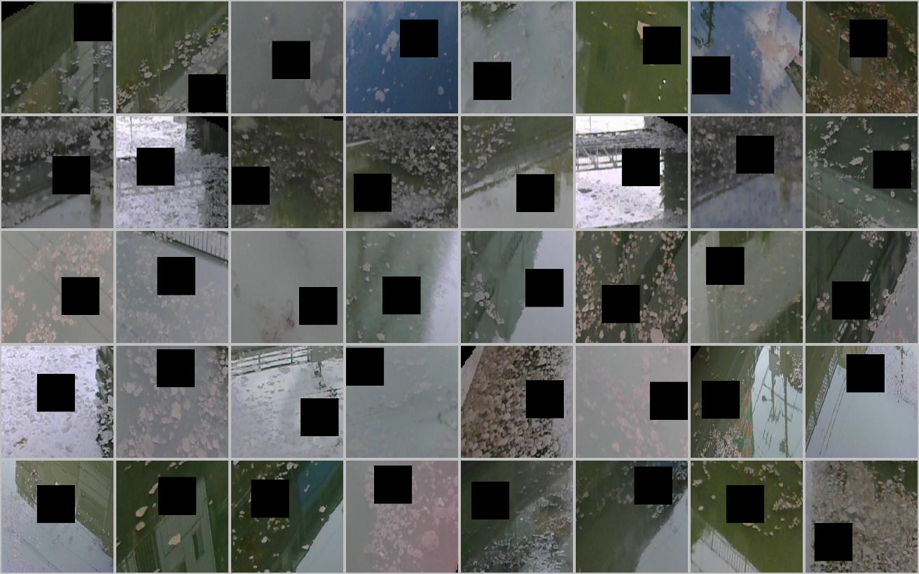
Figure 4: Cutout Augmented Images of Scum grow-thick class

As illustrated in Fig.5, RICAP involves mixing four randomly cropped images, respectively, and concatenating them into a new augmented image. RICAP greatly expands the variety of images and prevents overfitting of deep CNNs. Image data manipulation is done in three steps. First, we can randomly select four images $m\in{1,2,3,4}$ from the practice dataset. On the upper left $(m=1)$, upper right $(m=2)$, lower left $(m=3)$, and lower right sides $(m=4)$, we patch them in that order. Second, we can crop the images separately. $\bar{w}$ and $\bar{h}$ denotes the width and height of the training image, respectively. We can randomly set the boundary position $(w,h)$ of the four images $m$ from a uniform distribution. This is known as the variant $anywhere$-RICAP.