Markovian Foundations for Quasi-Stochastic Approximation
with Applications to Extremum Seeking Control

Abstract

This paper concerns quasi-stochastic approximation (QSA) to solve root finding problems commonly found in applications to optimization and reinforcement learning. The general constant gain algorithm may be expressed as the time-inhomogeneous ODE ${\mathchoice{\genfrac{}{}{}{1}{d}{dt}}{\genfrac{}{}{}{1}{d}{dt}}{\genfrac{}{}{}{3}{d}{dt}}{\genfrac{}{}{}{3}{d}{dt}}}\Uptheta_{t}=\alpha f_{t}(\Uptheta_{t})$, with state process $\Uptheta$ evolving on $\mathbb{R}^{n}$. Theory is based on an almost periodic vector field, so that in particular the time average of $f_{t}(\theta)$ defines the time-homogeneous mean vector field ${\widebar{f}}\colon\mathbb{R}^{d}\to\mathbb{R}^{d}$ with ${\widebar{f}}(\theta^{*})={\mathchoice{{\mathchoice{\mbox{\large\sf 0}}{\mbox{\large\sf 0}}{\mbox{\tiny\sf 0}}{\mbox{\tiny\sf 0}}}}{\mbox{\sf 0}}{\mbox{\tiny\sf 0}}{\mbox{\tiny\sf 0}}}$. Under smoothness assumptions on the functions involved, the following exact representation is obtained:

$${\mathchoice{\genfrac{}{}{}{1}{d}{dt}}{\genfrac{}{}{}{1}{d}{dt}}{\genfrac{}{}{}{3}{d}{dt}}{\genfrac{}{}{}{3}{d}{dt}}}\Uptheta_{t}=\alpha[{\widebar{f}}(\Uptheta_{t})-\alpha\widebar{\Upupsilon}_{t}+\alpha^{2}{\cal W}_{t}^{0}+\alpha\frac{d}{dt}{\cal W}_{t}^{1}+\frac{d^{2}}{dt^{2}}{\cal W}_{t}^{2}]$$

along with formulae for the smooth signals $\{\widebar{\Upupsilon}_{t},{\cal W}_{t}^{i}:i=0,1,2\}$. This representation is based on the application of techniques from Markov processes, for which Poisson’s equation plays a central role. This new representation, combined with new conditions for ultimate boundedness, has many applications for furthering the theory of QSA and its applications, including the following implications that are developed in this paper:

• A proof that the estimation error $\|\Uptheta_{t}-\theta^{*}\|$ is of order $O(\alpha)$, but can be reduced to $O(\alpha^{2})$ using a second order linear filter.

• In application to extremum seeking control [an approach to gradient free optimization], it is found that the results do not apply because the standard algorithms are not Lipschitz continuous. A new approach is presented to ensure that the required Lipschitz bounds hold, and from this we obtain stability, transient bounds, asymptotic bias of order $O(\alpha^{2})$, and asymptotic variance of order $O(\alpha^{4})$.

• It is in general possible to obtain better than $O(\alpha)$ bounds on error in traditional stochastic approximation when there is Markovian noise.

AMS-MSC: 68T05 (Primary), 93E35, 49L20 (Secondary)

1 Introduction

The basic problem of interest in this paper is root finding: find or approximate a solution $\theta^{*}\in\mathbb{R}^{d}$ to ${\widebar{f}}(\theta^{*})=0$, where ${\widebar{f}}\colon\mathbb{R}^{d}\to\mathbb{R}^{d}$ may not be available in closed form, but noisy measurements of ${\widebar{f}}(\theta)$ are available for any $\theta$. There is a large library of solution techniques.

1.1 Root finding with noisy observations

The field of stochastic approximation (SA) was born in the work of Robbins and Monro [48]. The goal is to solve the root finding problem in which the function ${\widebar{f}}\colon\mathbb{R}^{d}\to\mathbb{R}^{d}$ is expressed as the expectation

$${\widebar{f}}(\theta)\mathbin{:=}{\sf E}[f(\theta,{\scalebox{1.1}{$\upxi$}})]$$ (1)

with $\upxi$ a random vector taking values in $\mathbb{R}^{m}$, and $f\colon\mathbb{R}^{d}\times\mathbb{R}^{m}\to\mathbb{R}^{d}$.

The basic SA algorithm is expressed as the $d$-dimensional recursion,

$$\theta_{n+1}=\theta_{n}+\alpha_{n+1}f(\theta_{n},{\scalebox{1.1}{$\upxi$}}_{n+1})\,,\qquad n\geq 0,$$ (2)

in which $\{\alpha_{n}\}$ is the non-negative step-size sequence, and ${\scalebox{1.1}{$\upxi$}}_{n+1}\buildrel\rm d\over{\longrightarrow}{\scalebox{1.1}{$\upxi$}}$ as $n\to\infty$. Writing $\widetilde{\Xi}_{n}=f(\theta_{n},{\scalebox{1.1}{$\upxi$}}_{n+1})-{\widebar{f}}(\theta_{n})$, the SA recursion can be expressed in the suggestive form,

$$\theta_{n+1}=\theta_{n}+\alpha_{n+1}\{{\widebar{f}}(\theta_{n})+\widetilde{\Xi}_{n}\}\,,\qquad n\geq 0$$ (3)

This is interpreted as a noisy Euler approximation of the ODE

$${\mathchoice{\genfrac{}{}{}{1}{d}{dt}}{\genfrac{}{}{}{1}{d}{dt}}{\genfrac{}{}{}{3}{d}{dt}}{\genfrac{}{}{}{3}{d}{dt}}}\upvartheta_{t}={\widebar{f}}(\upvartheta_{t})$$ (4)

Convergence theory for SA is based on the recognition that the identity ${\widebar{f}}(\theta^{*})=0$ means that $\theta^{*}$ is the stationary point for this ODE. Convergence of the SA recursion is established under the assumption that (4) is globally asymptotically stable, along with some regularity conditions on the noise, and the standard assumptions ensuring success of noiseless Euler approximations [7]. Note that in early work it was assumed that the sequence ${\scalebox{1.1}{$\bm{\upxi}$}}\mathbin{:=}\{{\scalebox{1.1}{$\upxi$}}_{n}:n\geq 1\}$ is i.i.d.  (independent and identically distributed). It is made clear in [7] that convergence does not require such strong assumptions; it is only when we turn to rates of convergence that we require strong assumptions and far more elaborate analysis.

While there have been exciting advances in SA theory over recent decades, these advances do not allow us to escape an unfortunate truth: in the majority of applications of SA, the mean square error decays no faster than $1/n$. There appears to be no way to avoid the Central Limit Theorem.

While this curse of variance is true in broad generality, there is a remedy made possible by the flexibility we have in many application domains, such as optimization and reinforcement learning: in these applications it is we who design the noise for purposes of “exploration”. We obtain much more efficient algorithms by abandoning randomness in the algorithm.

It is also convenient to perform analysis in continuous time, so that the recursion (2) is replaced with an ordinary differential equation.

Quasi-Stochastic Approximation  is a deterministic analog of stochastic approximation. The QSA ODE is defined by the ordinary differential equation

$${\mathchoice{\genfrac{}{}{}{1}{d}{dt}}{\genfrac{}{}{}{1}{d}{dt}}{\genfrac{}{}{}{3}{d}{dt}}{\genfrac{}{}{}{3}{d}{dt}}}\Uptheta_{t}=a_{t}f(\Uptheta_{t},{\scalebox{1.1}{$\upxi$}}_{t})$$ (5)

where $f\colon\mathbb{R}^{d}\times\mathbb{R}^{m}\to\mathbb{R}^{d}$ is continuous. The $m$-dimensional deterministic continuous time process $\bm{\upxi}$ is called the probing signal.

Subject to mild assumptions, it was shown in [26] that the algorithm can be designed so that the squared error decays at rate $1/t^{4\rho}$ for the vanishing gain algorithm, using

$$a_{t}=\alpha/(1+t/t_{e})^{\rho}$$ (6)

with $\rho\in({\mathchoice{\genfrac{}{}{}{1}{1}{2}}{\genfrac{}{}{}{1}{1}{2}}{\genfrac{}{}{}{3}{1}{2}}{\genfrac{}{}{}{3}{1}{2}}},1)$, and $\alpha>0$, $t_{e}\geq 1$ arbitrary constants.

The present article focuses on the case $\rho=0$, meaning the gain is constant: $a_{t}\equiv\alpha$.

It is assumed throughout the paper that the probing signal is a nonlinear function of sinusoids: ${\scalebox{1.1}{$\upxi$}}_{t}=G_{0}({\scalebox{1.1}{$\upxi$}}_{t}^{0})$, with $G_{0}\colon\mathbb{R}^{K}\to\mathbb{R}^{m}$ continuous, and

$${\scalebox{1.1}{$\upxi$}}_{t}^{0}=[\cos(2\pi[\,\omega_{1}t+\phi_{1}]);\,\dots;\,\cos(2\pi[\,\omega_{K}t+\phi_{K}])]$$ (7)

Motivation for a nonlinearity may be to create rich probing signals from simple ones. For example, with $K=1$ we can obtain ${\scalebox{1.1}{$\upxi$}}_{t}=[\cos(2\pi\omega_{1}t);\,\cos(4\pi\omega_{1}t);\,\dots;\,\cos(2m\pi\omega_{1}t)]$ for any $m\geq 1$, with $G_{0}\colon\mathbb{R}\to\mathbb{R}^{m}$ polynomial. On choosing $G_{0}$ linear we obtain, for vectors $\{v^{i}\}\subset\mathbb{R}^{m}$,

$${\scalebox{1.1}{$\upxi$}}_{t}=\sum_{i=1}^{K}v^{i}\cos(2\pi[\omega_{i}t+\phi_{i}])$$ (8)

For analysis it is crucial to abandon ${\scalebox{1.1}{$\upxi$}}_{t}^{0}$ in favor of the $K$-dimensional clock-process $\Phi$ with entries $\Phi_{t}^{i}=\exp(2\pi j[\omega_{i}t+\phi_{i}])$. On defining $G(z)=G_{0}((z+1/z)/2)$, where $1/z\mathbin{:=}(1/z_{1},\dots,1/z_{K})$ for $z\in\{\mathbb{C}\setminus\{0\}\}^{K}$, we obtain

$${\scalebox{1.1}{$\upxi$}}_{t}=G(\Phi_{t})$$ (9)

The function $G$ will be assumed continuous on the restricted domain $\{\mathbb{C}\setminus\{0\}\}^{K}$.

The clock-process $\Phi$ is Markovian. It can also be expressed as the solution to the linear system,

$${\mathchoice{\genfrac{}{}{}{1}{d}{dt}}{\genfrac{}{}{}{1}{d}{dt}}{\genfrac{}{}{}{3}{d}{dt}}{\genfrac{}{}{}{3}{d}{dt}}}\Phi_{t}=W\Phi_{t},\quad\text{with }W=2\pi j\hbox{\rm diag\thinspace}(\omega_{i})$$ (10)

It evolves on a compact subset of Euclidean space denoted $\Upomega\subset\mathbb{C}^{K}$, and it is evident that the uniform distribution on $\Upomega$ is the unique invariant measure for $\Phi$; this is denoted $\uppi$.

The mean vector field associated with (5) is defined as the expectation,

$${\widebar{f}}(\theta)={\sf E}[f(\theta,G(\Phi))]\,,\qquad\theta\in\mathbb{R}^{d}\,,\qquad\textit{in which $\Phi\sim\uppi$. }$$ (11)

1.2 Perturbative mean flow

The central conclusion on which most of the concepts in this paper are based upon is the following representation for the QSA ODE, which holds under smoothness conditions on $f$ and $G_{0}$.

Perturbative Mean Flow:  The solution to the QSA ODE admits the exact description

$${\mathchoice{\genfrac{}{}{}{1}{d}{dt}}{\genfrac{}{}{}{1}{d}{dt}}{\genfrac{}{}{}{3}{d}{dt}}{\genfrac{}{}{}{3}{d}{dt}}}\Uptheta_{t} =\alpha[{\widebar{f}}(\Uptheta_{t})-\alpha\widebar{\Upupsilon}_{t}+{\cal W}_{t}]$$ (12)

$$\qquad{\cal W}_{t}=\alpha^{2}{\cal W}_{t}^{0}+\alpha\frac{d}{dt}{\cal W}_{t}^{1}+\frac{d^{2}}{dt^{2}}{\cal W}_{t}^{2}$$

The details:

• The deterministic processes $\{{\cal W}_{t}^{i}:i=0,1,2\}$ have explicit representations, given in (44a)–(44c), as smooth functions of the larger state process ${\mathchoice{\mbox{\boldmath$\Psi$}}{\mbox{\boldmath$\Psi$}}{\mbox{\boldmath$\scriptstyle\Psi$}}{\mbox{\boldmath$\scriptscriptstyle\Psi$}}}=(\bm{\Uptheta},{\mathchoice{\mbox{\boldmath$\Phi$}}{\mbox{\boldmath$\Phi$}}{\mbox{\boldmath$\scriptstyle\Phi$}}{\mbox{\boldmath$\scriptscriptstyle\Phi$}}})$.

• The function $\widebar{\Upupsilon}_{t}=\widebar{\Upupsilon}(\Uptheta_{t})$ appears when there is multiplicative noise in the QSA ODE. It can contribute significantly to the estimation error $\|\Uptheta_{t}-\theta^{*}\|$, resulting in large bias and variance. Fortunately, it can be eliminated with careful design.

The implications of the perturbative mean flow (or P-mean flow) representation to algorithm design are focuses of this paper.

However, there is one catch: while the P-mean flow representation holds in broad generality, we cannot use it to establish stability (in the sense of ultimate boundedness) since to-date we have not found global Lipschitz bounds on the functions $\{\widebar{\Upupsilon},{\cal W}^{i}:i=0,1,2\}$.

Algorithm Performance:  The pair ${\mathchoice{\mbox{\boldmath$\Psi$}}{\mbox{\boldmath$\Psi$}}{\mbox{\boldmath$\scriptstyle\Psi$}}{\mbox{\boldmath$\scriptscriptstyle\Psi$}}}=(\bm{\Uptheta},{\mathchoice{\mbox{\boldmath$\Phi$}}{\mbox{\boldmath$\Phi$}}{\mbox{\boldmath$\scriptstyle\Phi$}}{\mbox{\boldmath$\scriptscriptstyle\Phi$}}})$ is a Feller Markov process. Existence of an invariant measure $\upvarpi\sim{\mathchoice{\mbox{\boldmath$\Psi$}}{\mbox{\boldmath$\Psi$}}{\mbox{\boldmath$\scriptstyle\Psi$}}{\mbox{\boldmath$\scriptscriptstyle\Psi$}}}$ is guaranteed for QSA whenever the sample path $\bm{\Uptheta}$ is bounded from at least one initial condition. It is not known if $\upvarpi$ is unique, so bias and variance are defined in terms of sample path averages

$$\beta_{\Uptheta} =\mathop{\rm lim{\,}sup}_{T\to\infty}\Bigl{\|}\frac{1}{T}\int_{0}^{T}[\Uptheta_{t}-\theta^{*}]\,dt\Bigr{\|}\,,$$ (13)

$$\sigma^{2}_{\Uptheta} =\Bigl{(}\mathop{\rm lim{\,}sup}_{T\to\infty}\frac{1}{T}\int_{0}^{T}\|\Uptheta_{t}-\theta^{*}\|^{2}\,dt\Bigr{)}-\|\beta_{\Uptheta}\|^{2}\,.$$

The standard $L_{p}$ norms are also considered in their sample path forms:

$$\|\Uptheta-\theta^{*}\|_{L_{1}}=\mathop{\rm lim{\,}sup}_{T\to\infty}\frac{1}{T}\int_{0}^{T}\|\Uptheta_{t}-\theta^{*}\|\,dt\,,$$ (14)

$$\|\Uptheta-\theta^{*}\|_{L_{2}}=\sqrt{\mathop{\rm lim{\,}sup}_{T\to\infty}\frac{1}{T}\int_{0}^{T}\|\Uptheta_{t}-\theta^{*}\|^{2}\,dt}\,.$$

The $L_{1}$ norm is also referred to as the absolute average error (AAD). These quantities are related via

$$\|\Uptheta-\theta^{*}\|_{L_{1}}\leq\|\Uptheta-\theta^{*}\|_{L_{2}}=\sqrt{\sigma^{2}_{\theta}+\beta_{\Uptheta}^{2}}\,.$$ (15)

We say that the AAD is $O(\eta_{\alpha})$ if there is a finite constant $B_{0}$ such that $\|\Uptheta-\theta^{*}\|_{L_{1}}\leq B_{0}\eta_{\alpha}$ for all $\alpha>0$ in a neighborhood of the origin; $\eta_{\alpha}$ will be polynomial in $\alpha$.

We find that the AAD of QSA may be order $O(\alpha)$ even when $\widebar{\Upupsilon}\equiv 0$. Fig. 1 illustrates how linear filtering techniques can reduce this AAD to $O(\alpha^{2})$. The concept is simple: if ${\mathchoice{\genfrac{}{}{}{1}{d}{dt}}{\genfrac{}{}{}{1}{d}{dt}}{\genfrac{}{}{}{3}{d}{dt}}{\genfrac{}{}{}{3}{d}{dt}}}u_{t}$ is passed through a low pass filter with bandwidth $\gamma>0$, then the output $y_{t}$ satisfies $|y_{t}|\leq\gamma\|{\mathchoice{\mbox{\boldmath$u$}}{\mbox{\boldmath$u$}}{\mbox{\boldmath$\scriptstyle u$}}{\mbox{\boldmath$\scriptscriptstyle u$}}}\|_{\infty}+o(1)$. In general we require a second order filter to attenuate the term $\frac{d^{2}}{dt^{2}}{\cal W}_{t}^{2}$ appearing in (12).

We are also interested in the target bias, defined as the sample average

$$b_{\bar{f}}\mathbin{:=}\lim_{T\to\infty}\frac{1}{T}\int_{0}^{T}{\widebar{f}}(\Uptheta_{t})\,dt$$ (16)

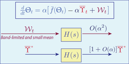
Figure 1: Perturbative mean flow and its implication to filter design.

1.3 Stability theory for QSA

We opt for the usual control-theoretic definition for the full state process: We say that ${\mathchoice{\mbox{\boldmath$\Psi$}}{\mbox{\boldmath$\Psi$}}{\mbox{\boldmath$\scriptstyle\Psi$}}{\mbox{\boldmath$\scriptscriptstyle\Psi$}}}=(\bm{\Uptheta},{\mathchoice{\mbox{\boldmath$\Phi$}}{\mbox{\boldmath$\Phi$}}{\mbox{\boldmath$\scriptstyle\Phi$}}{\mbox{\boldmath$\scriptscriptstyle\Phi$}}})$ is ultimately bounded if there is a fixed constant $B<\infty$ satisfying the following: for each initial condition $\Uptheta_{0}=\theta$, $\Phi_{0}=z$, there is a finite time $t_{0}=t_{0}(\theta,z)$ such that

$$\|\Uptheta_{t}\|\leq B\,,\qquad t\geq t_{0}$$ (17)

Two criteria to establish this property are available based entirely on the mean vector field ${\widebar{f}}$:

• Lipschitz Lyapunov Function: For a $C^{1}$ function $V\colon\mathbb{R}^{d}\to\mathbb{R}_{+}$ and a constant $\delta_{0}>0$,

  $$\frac{d}{dt}V(\upvartheta_{t})\leq-\delta_{0}V(\upvartheta_{t})\,,\qquad\textit{when $\|\upvartheta_{t}\|\geq\delta_{0}^{-1}$}$$ (18)

  This is equivalently expressed $\nabla V(\theta)\cdot{\widebar{f}}(\theta)\leq-\delta_{0}V(\theta)$ for all $\|\theta\|\geq\delta_{0}^{-1}$. This implies a similar bound for the QSA ODE under very general conditions. Most crucial is that $f$, ${\widebar{f}}$, and $V$ each satisfy a global Lipschitz bound.

• ODE@$\infty$: This is the vector field obtained by scaling

  $${\widebar{f}}_{\infty}(\theta)\mathbin{:=}\lim_{r\to\infty}{\widebar{f}}^{r}(\theta)\quad\textit{with}\quad{\widebar{f}}^{r}(\theta)=r^{-1}{\widebar{f}}(r\theta)\,,\qquad\theta\in\mathbb{R}^{d}$$ (19)

  If this exists, and if the ODE with this vector field is locally asymptotically stable, then we establish a relaxation of (18) that also implies that $\Psi$ is ultimately bounded.

The first criterion might look odd to those accustomed to quadratic Lyapunov functions. Suppose that $V_{1}$ is quadratic, of the form $V_{1}(\theta)=\theta^{\intercal}P\theta$ with $P>0$ $(d\times d)$, and solves $\nabla V_{1}(\theta)\cdot{\widebar{f}}(\theta)\leq-\delta_{1}V_{1}(\theta)$ for some $\delta_{1}>0$ and all $\|\theta\|\geq\delta_{1}^{-1}$. It follows from the chain rule that (18) holds using $V=\sqrt{1+V_{1}}$, and $\delta_{0}\in(\delta_{1}/2,1)$.

The second approach is based on the very notion of ultimate boundedness: if this condition fails to hold, then by definition the state blows up. Hence we look at the evolution on a compressed spatial scale. An example is shown in Fig. 2, with details postponed to Section 3.

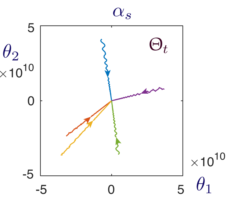
Figure 2: Solutions to extremum seeking control for the Rastrigin objective, starting from very large initial conditions

The ODE@$\infty$ is also a useful technique to establish ultimate boundedness of the mean flow: consider a large initial condition, with magnitude $r=\|\upvartheta_{0}\|$. The scaled state process $\upvartheta^{r}_{t}=r^{-1}\upvartheta_{t}$ solves the scaled ODE,

$${\mathchoice{\genfrac{}{}{}{1}{d}{dt}}{\genfrac{}{}{}{1}{d}{dt}}{\genfrac{}{}{}{3}{d}{dt}}{\genfrac{}{}{}{3}{d}{dt}}}\upvartheta^{r}_{t}=r^{-1}{\widebar{f}}(\upvartheta_{t})={\widebar{f}}^{r}(\upvartheta_{t}^{r})\,,\qquad\|\upvartheta^{r}_{0}\|=1$$ (20)

This simple conclusion leads to a proof of ultimate boundedness for the mean flow, following two observations:

(i)  The convergence in (19) is uniform on compact subsets of $\mathbb{R}^{d}$ (an application of Lipschitz continuity).

(ii)  if ${\widebar{f}}_{\infty}$ is locally asymptotically stable, then it must be globally exponentially asymptotically stable, with the origin the unique stationary point, ${\widebar{f}}_{\infty}({\mathchoice{{\mathchoice{\mbox{\large\sf 0}}{\mbox{\large\sf 0}}{\mbox{\tiny\sf 0}}{\mbox{\tiny\sf 0}}}}{\mbox{\sf 0}}{\mbox{\tiny\sf 0}}{\mbox{\tiny\sf 0}}})={\mathchoice{{\mathchoice{\mbox{\large\sf 0}}{\mbox{\large\sf 0}}{\mbox{\tiny\sf 0}}{\mbox{\tiny\sf 0}}}}{\mbox{\sf 0}}{\mbox{\tiny\sf 0}}{\mbox{\tiny\sf 0}}}$.

Based on these conclusions we obtain semi-exponential stability, in the following sense: for some $\delta_{e}>0$ and initial conditions satisfying $\|\upvartheta_{0}\|\geq\delta_{e}^{-1}$, solutions to (4) satisfy

$$V(\upvartheta_{t})\leq V(\upvartheta_{0})e^{-\delta_{e}t}\,,\qquad 0\leq t\leq T(\upvartheta_{0})$$ (21)

where $T$ is the first entrance time: $T(\upvartheta_{0})\mathbin{:=}\min\{t\geq 0:\|\upvartheta_{t}\|\leq\delta_{e}^{-1}\}$.

The bound (21) is extended to the QSA ODE in Thm. 2.9, under either of these two stability criteria.

1.4 Bridge building

As motivation, to provide examples, and to provide a short literature survey, we present a brief survey of gradient free optimization (GFO) and how it is related to QSA and extremum seeking control (ESC). The definition of ESC is postponed to Section 3, based on interpretation of its standard block diagram description shown in Fig. 3.

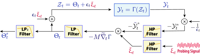
Figure 3: A Typical Architecture for Extremum Seeking Control for Gradient-Free Optimization

1.4.1 SPSA

Within the area of GFO two algorithms of Spall are most easily described and justified. Each are SA algorithms of the form (2), differing only in the definition of $f$:

$$\text{\sf 1SPSA:}\quad f(\theta,{\scalebox{1.1}{$\upxi$}}) =-\frac{1}{\varepsilon}{\scalebox{1.1}{$\upxi$}}\Upgamma(\theta+\varepsilon{\scalebox{1.1}{$\upxi$}})$$ (22a)

$$\text{\sf 2SPSA:}\quad f(\theta,{\scalebox{1.1}{$\upxi$}}) =-\frac{1}{2\varepsilon}{\scalebox{1.1}{$\upxi$}}\bigl{[}\Upgamma(\theta+\varepsilon{\scalebox{1.1}{$\upxi$}})-\Upgamma(\theta-\varepsilon{\scalebox{1.1}{$\upxi$}})\bigr{]}$$ (22b)

It is assumed that the probing sequence $\{{\scalebox{1.1}{$\upxi$}}_{n}\}$ is i.i.d., and in much of the theory it is assumed that the entries of ${\scalebox{1.1}{$\upxi$}}_{n}$ have support in $\{-1,1\}$. In either case, the mean vector field is defined via (1):

$${\widebar{f}}(\theta)\mathbin{:=}{\sf E}[f(\theta,{\scalebox{1.1}{$\upxi$}}_{n+1})]\,,\qquad\theta\in\mathbb{R}^{d}$$

This is independent of $n$ under the assumption that the probing sequence is i.i.d..

Motivation for either is usually based on a first-order Taylor series approximation. The following exact representations follow from the Fundamental Theorem of Calculus:

$$\text{\sf 1SPSA:}\quad f(\theta,{\scalebox{1.1}{$\upxi$}}) =-{\scalebox{1.1}{$\upxi$}}{\scalebox{1.1}{$\upxi$}}^{\intercal}\frac{1}{\varepsilon}\int_{0}^{\varepsilon}\nabla\Upgamma\,(\theta+t{\scalebox{1.1}{$\upxi$}})\,dt-\frac{1}{\varepsilon}{\scalebox{1.1}{$\upxi$}}\Upgamma(\theta)$$ (23a)

$$\text{\sf 2SPSA:}\quad f(\theta,{\scalebox{1.1}{$\upxi$}}) =-{\scalebox{1.1}{$\upxi$}}{\scalebox{1.1}{$\upxi$}}^{\intercal}\frac{1}{2\varepsilon}\int_{-\varepsilon}^{\varepsilon}\nabla\Upgamma\,(\theta+t{\scalebox{1.1}{$\upxi$}})\,dt$$ (23b)

These representations in terms of average gradients provide the first step in the proof of the following:

Proposition 1.1.

Suppose that the $d$-dimensional sequence $\bm{\upxi}$ is i.i.d. with zero mean, and that ${\scalebox{1.1}{$\upxi$}}_{n+1}\buildrel\rm dist\over{=}-{\scalebox{1.1}{$\upxi$}}_{n+1}$ (equality in distribution). Then the mean vector fields for 1SPSA and 2SPSA coincide.

Suppose in addition that the objective $\Upgamma$ is continuously differentiable ($C^{1}$) and strongly convex in a neighborhood of the optimizer $\theta^{\text{\tiny\sf opt}}$. Then, there exists $\varepsilon^{0}>0$ such that the function ${\widebar{f}}$ has a root $\theta^{*}$ for $0<\varepsilon\leq\varepsilon^{0}$, and for either 1SPSA or 2SPSA,

$$\|\theta^{*}-\theta^{\text{\tiny\sf opt}}\|=O(\varepsilon^{2})\qquad\textit{and}\qquad\Upgamma(\theta^{*})-\Upgamma(\theta^{\text{\tiny\sf opt}})=O(\varepsilon^{4})$$ (24)

$\sqcap$$\sqcup$

SPSA is a perfect example of a successful algorithm that can be improved using deterministic exploration.

1.4.2 ESC and QSA

Spall’s SPSA recursions admit natural analogs as QSA ODEs, with vector fields

$$\text{\sf 1qSGD:}\quad f(\Uptheta_{t},{\scalebox{1.1}{$\upxi$}}_{t}) =-\frac{1}{\varepsilon}{\scalebox{1.1}{$\upxi$}}_{t}\Upgamma(\Uptheta_{t}+\varepsilon{\scalebox{1.1}{$\upxi$}}_{t})$$ (25a)

$$\text{\sf 2qSGD:}\quad f(\Uptheta_{t},{\scalebox{1.1}{$\upxi$}}_{t}) =-\frac{1}{2\varepsilon}{\scalebox{1.1}{$\upxi$}}_{t}\bigl{[}\Upgamma(\Uptheta_{t}+\varepsilon{\scalebox{1.1}{$\upxi$}}_{t})-\Upgamma(\Uptheta_{t}-\varepsilon{\scalebox{1.1}{$\upxi$}}_{t})\bigr{]}$$ (25b)

in which qSGD refers to quasi-stochastic gradient descent. In examples that follow we typically take the sinusoidal probing signal (8).

In Section 3 we show that 1qSGD is a simple instance of extremum seeking control.

And we also find a challenge: in both domains, ESC and 1qSGD, convergence theory is limited because the vector field $f$ is not Lipschitz continuous in its first variable. Lipschitz continuity is a critical component of theory for both SA and QSA. A remedy is introduced in this paper, through the introduction of a state-depending probing gain. Details are found in Section 3.2.

1.4.3 Averaging

The theory of averaging for variance reduction is well-established in the SA literature, with application to optimization [19, 38, 37] and to GFO [51]. The idea is very simple: given the estimates $\{\theta_{n}:0\leq n\leq N\}$ from any SA recursion, obtain a new estimate via

$$\theta^{\text{\tiny\sf PR}}_{N}\mathbin{:=}\frac{1}{N-N_{0}}\sum_{n=N_{0}+1}^{N}\theta_{n}$$ (26)

where $1\leq N_{0}<N$ is chosen to discard large transients. This apparently simple “hack” provides enormous benefit: under mild conditions, the variance of this estimate of $\theta^{*}$ is minimal in a strong sense [7, 23]. The technique goes by the name of Polyak-Ruppert averaging in honor of the creators of the technique and original analysis [49, 42, 43] (note Polyak’s contributions in [42] prior to his collaboration with Juditsky). The article [13] is an early application of these ideas to accelerate GFO.

This is similar to the low pass filter shown in (3), generating $\Uptheta^{\text{\tiny\sf F}}_{t}$ from $\Uptheta_{t}$. We will find better options for fixed gain QSA in Section 2.3.

1.4.4 Multiplicative noise

One objective of this paper is to bring to light the challenges posed by multiplicative noise. Many optimistic results in prior work consider additive noise models for which the nuisance term $\Upupsilon$ is not present:

• Estimation error bounds of order $O(\alpha^{2})$ are obtained in [2] for ESC when the objective is quadratic.

• There are recent optimistic results in the stochastic approximation literature for fixed gain algorithms [37, 16]. Through design it is possible to obtain zero asymptotic bias and optimize variance (via averaging). These results are obtained for models with additive white noise.

For QSA we obtain both $O(\alpha^{2})$ bounds for AAD and target bias through careful design of filters and the probing signal. Theory shows that we cannot expect $O(\alpha^{2})$ AAD for general models, unless a filter is designed following the specifications in Thm. 2.7.

In stochastic settings with Markovian noise it is not at all clear how to obtain such strong conclusions—averaging cannot remove the inherent $O(\alpha)$ AAD that is a consequence of statistical memory. Details are found in Section 2.5.3.

Overview  The remainder of the body of the paper is organized into five additional sections: The main technical results of the paper are contained in Section 2, including a proof of the P-mean flow representation (12). Implications to extremum seeking control are summarized in Section 3, with examples in Section 4, and conclusions and directions for future research are summarized in Section 5. A literature survey is contained in Section 6, and proofs of some technical results are contained in the Appendix.

2 QSA Theory

The theory described in this section is based on the fixed-gain QSA ODE with $a_{t}\equiv\alpha>0$:

$${\mathchoice{\genfrac{}{}{}{1}{d}{dt}}{\genfrac{}{}{}{1}{d}{dt}}{\genfrac{}{}{}{3}{d}{dt}}{\genfrac{}{}{}{3}{d}{dt}}}\Uptheta_{t}=\alpha f(\Uptheta_{t},{\scalebox{1.1}{$\upxi$}}_{t})$$ (27)

Convergence of $\{\Uptheta_{t}\}$ to $\theta^{*}$ cannot be expected; instead with careful design of the algorithm we obtain bounds on asymptotic bias of order $O(\alpha^{2})$ and variance of order $O(\alpha^{4})$.

2.1 Markovian framework for analysis

In the theory of SA the stochastic sequence $\{{\scalebox{1.1}{$\upxi$}}_{n+1}\}$ appearing in (2) is not always assumed to be i.i.d.. Sharp results on asymptotic variance are available when it can be expressed as a function of a well behaved Markov chain. It may come as a big surprise to learn that the techniques extend to QSA analysis, and the application of techniques rooted in Markov chain theory are the only tools available to obtain (12) and its progeny.

For the fixed gain QSA ODE it is clear that the pair ${\mathchoice{\mbox{\boldmath$\Psi$}}{\mbox{\boldmath$\Psi$}}{\mbox{\boldmath$\scriptstyle\Psi$}}{\mbox{\boldmath$\scriptscriptstyle\Psi$}}}=(\bm{\Uptheta},{\mathchoice{\mbox{\boldmath$\Phi$}}{\mbox{\boldmath$\Phi$}}{\mbox{\boldmath$\scriptstyle\Phi$}}{\mbox{\boldmath$\scriptscriptstyle\Phi$}}})$ is itself the state process for a time-homogeneous dynamical system. It can also be regarded as a Feller Markov process on the closed state space $\Uppi=\mathbb{R}^{d}\times\Upomega$. Provided $\Psi$ is ultimately bounded, it admits at least one invariant measure [35, Thm. 12.1.2], which we denote $\upvarpi$. This is valuable conceptually, and in terms of notation. We can unambiguously write ${\widebar{g}}\mathbin{:=}{\sf E}[g(\Uptheta,{\scalebox{1.1}{$\upxi$}})]$ for a function $g\colon\mathbb{R}^{d}\times\mathbb{R}^{K}\to\mathbb{R}$, where the expectation is with respect to $\Psi\sim\upvarpi$.

The following simple result will aid in interpretation of other expectations. For any function $h\colon\Uppi\to\mathbb{R}$ that is continuously differentiable, define the continuous function $\mathcal{D}h$ via

$$\mathcal{D}h\,(\theta,z)\mathbin{:=}\partial_{\theta}h\,(\theta,z)\cdot f(\theta,G(z))+\partial_{z}h\,(\theta,z)\cdot Wz\,,\qquad(\theta,z)\in\Uppi$$ (28)

In Markov terminology, the functional $\mathcal{D}$ is known as the differential generator for $\Psi$.

Proposition 2.1.

Let $h\colon\Uppi\to\mathbb{R}$ be a $C^{1}$ function, and denote $g=\mathcal{D}h$. The following then hold:

• $g(\Psi_{t})={\mathchoice{\genfrac{}{}{}{1}{d}{dt}}{\genfrac{}{}{}{1}{d}{dt}}{\genfrac{}{}{}{3}{d}{dt}}{\genfrac{}{}{}{3}{d}{dt}}}h(\Psi_{t})$.

• Suppose that for some initial condition $\Psi_{0}$, the resulting trajectory $\{\Psi_{t}:t\geq 0\}$ is uniformly bounded. Then,

  $$\lim_{T\to\infty}\frac{1}{T}\int_{0}^{T}g(\Psi_{t})\,dt={\mathchoice{{\mathchoice{\mbox{\large\sf 0}}{\mbox{\large\sf 0}}{\mbox{\tiny\sf 0}}{\mbox{\tiny\sf 0}}}}{\mbox{\sf 0}}{\mbox{\tiny\sf 0}}{\mbox{\tiny\sf 0}}}$$

• Suppose that an invariant measure $\upvarpi$ exists with compact support. Then ${\sf E}[g(\Psi)]=0$ when $(\Uptheta,\Phi)=\Psi\sim\upvarpi$. In particular, on choosing $h(\theta,z)\equiv\theta$,

  $${\sf E}[f(\Uptheta,G(\Phi))]={\mathchoice{{\mathchoice{\mbox{\large\sf 0}}{\mbox{\large\sf 0}}{\mbox{\tiny\sf 0}}{\mbox{\tiny\sf 0}}}}{\mbox{\sf 0}}{\mbox{\tiny\sf 0}}{\mbox{\tiny\sf 0}}}$$ (29)

  $\sqcap$$\sqcup$

Proof.

Part (i) follows from the chain rule, and (ii) from the fundamental theorem of calculus:

$$h(\Psi_{T})=h(\Psi_{0})+\int_{0}^{T}g(\Psi_{t})\,dt\,,\qquad T>0$$

Part (iii) also follows from the fundamental theorem of calculus, using the expression above, but with a random initial condition. Choose $\Psi_{0}=(\Uptheta_{0},\Phi_{0})$ to be a $\Uppi$-valued random variable with distribution $\upvarpi$. We then have $\Psi_{t}\sim\upvarpi$ for all $t$. Taking expectations of each side completes the proof:

$${\sf E}[h(\Psi_{0})]={\sf E}[h(\Psi_{0})]+T{\sf E}[g(\Psi_{0})]$$

$\sqcap$$\sqcup$

Our main motivation for a Markovian framework comes from the application of solutions to Poisson’s equation: for functions $g,\,{\hat{g}}\colon\Upomega\to\mathbb{R}$, this is expressed

$${\hat{g}}(\Phi_{0})={\hat{g}}(\Phi_{T})+\int_{0}^{T}\tilde{g}(\Phi_{t})\,dt\,,\qquad T\geq 0\,,$$ (30)

where $\tilde{g}(z)=g(z)-{\widebar{g}}$ for $z\in\Upomega$, with ${\widebar{g}}$ the steady-state mean. We say that ${\hat{g}}$ is the solution to Poisson’s equation, and that $g$ is the forcing function. If ${\hat{g}}$ is continuously differentiable, then from (10) we obtain $\nabla^{\intercal}{\hat{g}}(z)Wz=-\tilde{g}(z)$ for $z\in\Upomega$.

Justification for smooth solutions to Poisson’s equation is obtained in [26] when the forcing function is analytic, and subject to assumptions on the frequencies defining $\Phi$. A review is contained in the Appendix, and a summary of required assumptions in Assumption (A0) below.

• Please note:

• The solution ${\hat{g}}$ is not unique. We always normalize so that ${\sf E}[{\hat{g}}(\Phi)]=0$.

• In the applications of Poisson’s equation used in this paper, it is frequently true that the function $g$ depends on $\Phi_{t}$ only through ${\scalebox{1.1}{$\upxi$}}_{t}$. This is this is not in general true for ${\hat{g}}$.

• Finally, on notation: we often write ${\hat{g}}_{t}$ instead of ${\hat{g}}(\Uptheta_{t},\Phi_{t})$ (similar notation for other functions of $\Psi$).

We will not require solutions for the joint process $\Psi$, but require a slight abuse of notation: for a vector-valued function on the joint state space $g\colon\Uppi\to\mathbb{R}$, we denote by ${\hat{g}}(\theta,\,\cdot\,)$ the solution to Poisson’s equation with $\theta\in\mathbb{R}^{d}$ fixed:

$${\hat{g}}(\theta,\Phi_{0})={\hat{g}}(\theta,\Phi_{T})+\int_{0}^{T}\tilde{g}(\theta,\Phi_{t})\,dt\,,\qquad T\geq 0\,.$$ (31)

This is applied with $g=f$ [the QSA ODE vector field (5)]; the solution ${\hat{f}}$ plays a part in the definition of $\widebar{\Upupsilon}$.

Further implications require a few assumptions and notation:

Assumptions  The following assumptions are in force throughout much of the paper.

The first assumption sets restrictions on frequencies: we begin with a “basis” of irrationally related frequencies specified as follows: For an integer $K_{0}$, frequencies $\{\omega_{1}^{0}\,,\dots\,,\omega_{K_{0}}^{0}\}$ are chosen of the following form:

$$\omega_{i}^{0}=\log(a_{i}/b_{i})>0\,,\ \ 1\leq i\leq K_{0}\,,\ \ \textit{where $\{a_{i},b_{i}\}$ are positive integers. }$$ (32)

$$\{\omega_{i}^{0}:1\leq i\leq K_{0}\}$$ are linearly independent over the field of rational numbers.

(A0a)  ${\scalebox{1.1}{$\upxi$}}_{t}=G_{0}({\scalebox{1.1}{$\upxi$}}_{t}^{0})$ for all $t$, with ${\scalebox{1.1}{$\upxi$}}_{t}^{0}$ defined in (7). The function $G_{0}\colon\mathbb{R}^{K}\to\mathbb{R}^{m}$ is assumed to be analytic, with the coefficients in the Taylor series expansion for $G_{0}({\scalebox{1.1}{$\upxi$}}_{t}^{0})$ absolutely summable.

(A0b)  The frequencies $\{\omega_{1}\,,\dots\,,\omega_{K}\}$ satisfy one of the two conditions:

Periodic: For a fixed but arbitrary frequency $\omega_{1}>0$ and an increasing sequence of positive integers $\{n_{i}\}$,

$$\omega_{i}=n_{i}\omega_{1}\,,\quad 2\leq i\leq K$$ (33a)

Transcendental Almost Periodic: The frequencies $\{\omega_{i}:1\leq i\leq K\}$ are positive, distinct, and in the positive integer span of the $\{\omega_{i}^{0}:1\leq i\leq K_{0}\}$:

$$\omega_{i}=\sum_{j}n_{i,j}\omega_{j}^{0}\quad\textit{ for integers $\{n_{i,j}\}\subset\mathbb{Z}_{+}$.}$$ (33b)

(A1)  The functions ${\widebar{f}}$ and $f$ are Lipschitz continuous: for a constant $L_{f}<\infty$,

$$\|{\widebar{f}}(\theta^{\prime})-{\widebar{f}}(\theta)\| \leq L_{f}\|\theta^{\prime}-\theta\|,$$ (34a)

$$\|f(\theta^{\prime},{\scalebox{1.1}{$\upxi$}})-f(\theta,{\scalebox{1.1}{$\upxi$}})\|+\|f(\theta,{\scalebox{1.1}{$\upxi$}}^{\prime})-f(\theta,{\scalebox{1.1}{$\upxi$}})\| \leq L_{f}\bigl{[}\|\theta^{\prime}-\theta\|+\|{\scalebox{1.1}{$\upxi$}}^{\prime}-{\scalebox{1.1}{$\upxi$}}\|\bigr{]}$$

for all $\theta^{\prime}\,,\theta\in\mathbb{R}^{d}$, ${\scalebox{1.1}{$\upxi$}}\,,{\scalebox{1.1}{$\upxi$}}^{\prime}\in\mathbb{R}^{m}$.

(A2)  The vector fields $f$ and ${\widebar{f}}$ are each twice continuously differentiable, with derivatives denoted

$$A(\theta,z) =\partial_{\theta}f\,(\theta,z)\,,\qquad{\bar{A}}(\theta)=\partial_{\theta}{\widebar{f}}\,(\theta)$$ (34b)

(A3)  There exists a solution ${\hat{f}}$ to Poisson’s equation that is continuously differentiable on $\Uppi$, and normalized so that ${\sf E}[{\hat{f}}(\theta,\Phi)]={\mathchoice{{\mathchoice{\mbox{\large\sf 0}}{\mbox{\large\sf 0}}{\mbox{\tiny\sf 0}}{\mbox{\tiny\sf 0}}}}{\mbox{\sf 0}}{\mbox{\tiny\sf 0}}{\mbox{\tiny\sf 0}}}$ for each $\theta$, with $\Phi\sim\uppi$. Its Jacobian with respect to $\theta$ is denoted

$$\widehat{A}(\theta,z)\mathbin{:=}\partial_{\theta}{\hat{f}}\,(\theta,z)$$ (34c)

Moreover, there are continuously differentiable solutions to Poisson’s equation for each of the two forcing functions ${\hat{f}}$ and $\Upupsilon$, with

$$\Upupsilon(\theta,z)=-\widehat{A}(\theta,z)f(\theta,G(z))$$ (34d)

The solutions are denoted, respectively, $\hat{\vphantom{\rule{1.0pt}{5.93056pt}}\smash{\hat{f}}}$ and $\widehat{\Upupsilon}$:

$$\hat{\vphantom{\rule{1.0pt}{5.93056pt}}\smash{\hat{f}}}(\theta,\Phi_{t_{0}}) =\int_{t_{0}}^{t_{1}}{\hat{f}}(\theta,\Phi_{t})\,dt+\hat{\vphantom{\rule{1.0pt}{5.93056pt}}\smash{\hat{f}}}(\theta,\Phi_{t_{1}})$$

$$\widehat{\Upupsilon}(\theta,\Phi_{t_{0}}) =\int_{t_{0}}^{t_{1}}[\Upupsilon(\theta,\Phi_{t})-\widebar{\Upupsilon}(\theta)]\,dt+\widehat{\Upupsilon}(\theta,\Phi_{t_{1}})\,, 0\leq t_{0}\leq t_{1}$$ (34e)

$$\textit{with}\quad\widebar{\Upupsilon}(\theta) ={\sf E}[\Upupsilon(\theta,\Phi)]=-\int_{\Upomega}\widehat{A}(\theta,z)f(\theta,G(z))\,\uppi(dz)\,, \theta\in\mathbb{R}^{d}$$

They are also normalized: ${\sf E}[\hat{\vphantom{\rule{1.0pt}{5.93056pt}}\smash{\hat{f}}}(\theta,\Phi)]={\sf E}[\widehat{\Upupsilon}(\theta,\Phi)]={\mathchoice{{\mathchoice{\mbox{\large\sf 0}}{\mbox{\large\sf 0}}{\mbox{\tiny\sf 0}}{\mbox{\tiny\sf 0}}}}{\mbox{\sf 0}}{\mbox{\tiny\sf 0}}{\mbox{\tiny\sf 0}}}$ for each $\theta$.     $\sqcap$$\sqcup$

Assumption (A0b) is justified in Section A.2, but deserves some explanation here. First, it would appear that (33a) is a special case of (33b) in which $K_{0}=1$. Note however that no restriction is placed on $\omega_{1}$ in (33a), except that it is strictly positive.

The assumption is imposed for two reasons:

• It is a sufficient condition ensuring that $\widebar{\Upupsilon}\equiv{\mathchoice{{\mathchoice{\mbox{\large\sf 0}}{\mbox{\large\sf 0}}{\mbox{\tiny\sf 0}}{\mbox{\tiny\sf 0}}}}{\mbox{\sf 0}}{\mbox{\tiny\sf 0}}{\mbox{\tiny\sf 0}}}$, assuming that Assumption (A3) holds so that $\Upupsilon$ is well defined. See the example following Thm. 2.7 to see that constraints on the frequencies are indeed needed for this.

• If $f(\theta,G(z))$ is an analytic function of $(\theta,z)$ on an appropriate domain, then Assumption (A3) holds.

Claim (i) is an application of Prop. 2.5; this result doesn’t require the full (A0b)—it is sufficient that the frequencies are distinct. Claim (ii) follows from Thm. A.5.

As for the remaining assumptions, we require (A1)–(A3) and further assumptions to obtain sharp bounds on bias and variance. In particular, the functions introduced in (A3) determine all of the terms in (12), with $\widebar{\Upupsilon}$ is defined in (34e).

The assumptions on $G_{0}$ in Assumption (A0a) are imposed so that the probing signal is almost periodic [1]. This combined with the Lipschitz conditions in (A1) imply a uniform version of the Law of Large Numbers:

Proposition 2.2.

Under (A0a) and (A1) the uniform Law of Large Numbers holds:

$$\lim_{T\to\infty}\sup_{\theta,z_{0}}\frac{1}{1+\|\theta\|}\left|\frac{1}{T}\int_{0}^{T}\bigl{[}f(\theta,{\scalebox{1.1}{$\upxi$}}_{t})-{\widebar{f}}(\theta)\bigr{]}\,dt\right|=0$$ (35)

where the supremum is over $\theta_{0}\in\mathbb{R}^{d}$, and initial conditions $\Phi_{0}=z_{0}\in\Upomega$.     $\sqcap$$\sqcup$

2.2 Three steps towards the perturbative mean flow

The notation in (34d) is complex, which brings us to the following compact alternative: For $h\colon\Uppi\to\mathbb{R}^{d}$ that is continuously differentiable in its first variable we let $D^{f}h$ denote its directional derivative in the direction $f$, where $f$ is the vector field for the QSA ODE:

$$[D^{f}h](\theta,z)=\partial_{\theta}h\,(\theta,z)\cdot f(\theta,G(z))\,,\qquad(\theta,z)\in\Uppi$$ (36)

This defines a component of the differential generator (28); recall from Prop. 2.1 that $g=\mathcal{D}h$ implies that $g(\Psi_{t})={\mathchoice{\genfrac{}{}{}{1}{d}{dt}}{\genfrac{}{}{}{1}{d}{dt}}{\genfrac{}{}{}{3}{d}{dt}}{\genfrac{}{}{}{3}{d}{dt}}}h(\Psi_{t})$.

The following companion to Prop. 2.1 will be used in the following: for any smooth solution to Poisson’s equation with forcing function $h\colon\Uppi\to\mathbb{R}$,

$${\mathchoice{\genfrac{}{}{}{1}{d}{dt}}{\genfrac{}{}{}{1}{d}{dt}}{\genfrac{}{}{}{3}{d}{dt}}{\genfrac{}{}{}{3}{d}{dt}}}{\hat{h}}(\Uptheta_{t},z) =\alpha[D^{f}{\hat{h}}](\Uptheta_{t},z)\,,\ z\in\Upomega$$ (37)

$${\mathchoice{\genfrac{}{}{}{1}{d}{dt}}{\genfrac{}{}{}{1}{d}{dt}}{\genfrac{}{}{}{3}{d}{dt}}{\genfrac{}{}{}{3}{d}{dt}}}{\hat{h}}(\Uptheta_{t},\Phi_{t}) =\alpha[D^{f}{\hat{h}}](\Uptheta_{t},\Phi_{t})-[h(\Uptheta_{t},\Phi_{t})-{\overline{h}}(\Uptheta_{t})]$$ (38)

Using $h={\hat{f}}$, the definition (34d) gives

$$\Upupsilon_{t}=-[D^{f}{\hat{f}}](\Uptheta_{t},\Phi_{t})=-\frac{1}{\alpha}\{{\mathchoice{\genfrac{}{}{}{1}{d}{dt}}{\genfrac{}{}{}{1}{d}{dt}}{\genfrac{}{}{}{3}{d}{dt}}{\genfrac{}{}{}{3}{d}{dt}}}{\hat{f}}_{t}+[f(\Uptheta_{t},{\scalebox{1.1}{$\upxi$}}_{t})-{\widebar{f}}(\Uptheta_{t})]\}$$ (39)

We now proceed through the three steps, with this representation in view:

$${\mathchoice{\genfrac{}{}{}{1}{d}{dt}}{\genfrac{}{}{}{1}{d}{dt}}{\genfrac{}{}{}{3}{d}{dt}}{\genfrac{}{}{}{3}{d}{dt}}}\Uptheta_{t}=\alpha\bigl{[}{\widebar{f}}(\Uptheta_{t})+\widetilde{\Xi}_{t}]\,,$$ (40)

where $\widetilde{\Xi}_{t}=f(\Uptheta_{t},{\scalebox{1.1}{$\upxi$}}_{t})-{\widebar{f}}(\Uptheta_{t})$ is called the apparent noise. Understanding (12) is equivalent to determining the functions $\{{\cal W}^{i}\}$ in the representation

$$\widetilde{\Xi}_{t} =-\alpha\widebar{\Upupsilon}_{t}+\alpha^{2}{\cal W}_{t}^{0}+\alpha{\mathchoice{\genfrac{}{}{}{1}{d}{dt}}{\genfrac{}{}{}{1}{d}{dt}}{\genfrac{}{}{}{3}{d}{dt}}{\genfrac{}{}{}{3}{d}{dt}}}{\cal W}_{t}^{1}+\tfrac{d^{2}}{dt^{2}}{\cal W}_{t}^{2}$$ (41)

Step 1:  Apply (38) with $g={\hat{f}}$:

$${\mathchoice{\genfrac{}{}{}{1}{d}{dt}}{\genfrac{}{}{}{1}{d}{dt}}{\genfrac{}{}{}{3}{d}{dt}}{\genfrac{}{}{}{3}{d}{dt}}}{\hat{f}}(\Uptheta_{t},\Phi_{t})=\partial_{\theta}{\hat{f}}(\Uptheta_{t},\Phi_{t}){\mathchoice{\genfrac{}{}{}{1}{d}{dt}}{\genfrac{}{}{}{1}{d}{dt}}{\genfrac{}{}{}{3}{d}{dt}}{\genfrac{}{}{}{3}{d}{dt}}}\Uptheta_{t}-[f(\Uptheta_{t},{\scalebox{1.1}{$\upxi$}}_{t})-{\widebar{f}}(\Uptheta_{t})]$$

This gives the first transformation of the apparent noise:

$$\widetilde{\Xi}_{t}=\underbrace{-{\mathchoice{\genfrac{}{}{}{1}{d}{dt}}{\genfrac{}{}{}{1}{d}{dt}}{\genfrac{}{}{}{3}{d}{dt}}{\genfrac{}{}{}{3}{d}{dt}}}{\hat{f}}(\Uptheta_{t},\Phi_{t})}_{\text{High pass}}+\underbrace{\alpha\partial_{\theta}{\hat{f}}(\Uptheta_{t},\Phi_{t})f(\Uptheta_{t},{\scalebox{1.1}{$\upxi$}}_{t})\phantom{{\mathchoice{\genfrac{}{}{}{1}{d}{dt}}{\genfrac{}{}{}{1}{d}{dt}}{\genfrac{}{}{}{3}{d}{dt}}{\genfrac{}{}{}{3}{d}{dt}}}}}_{\text{Attenuation}}$$

Recalling (34d) gives in shorthand notation,

$$\widetilde{\Xi}_{t}=-{\mathchoice{\genfrac{}{}{}{1}{d}{dt}}{\genfrac{}{}{}{1}{d}{dt}}{\genfrac{}{}{}{3}{d}{dt}}{\genfrac{}{}{}{3}{d}{dt}}}{\hat{f}}_{t}-\alpha\Upupsilon_{t}$$ (42)

Step 2:  Repeat previous argument with ${\hat{f}}$:

$${\mathchoice{\genfrac{}{}{}{1}{d}{dt}}{\genfrac{}{}{}{1}{d}{dt}}{\genfrac{}{}{}{3}{d}{dt}}{\genfrac{}{}{}{3}{d}{dt}}}\hat{\vphantom{\rule{1.0pt}{5.93056pt}}\smash{\hat{f}}}(\Uptheta_{t},\Phi_{t}) =\alpha[D^{f}\hat{\vphantom{\rule{1.0pt}{5.93056pt}}\smash{\hat{f}}}](\Uptheta_{t},\Phi_{t})-{\hat{f}}_{t}$$

$$\Rightarrow{\hat{f}}_{t}=\alpha[D^{f}\hat{\vphantom{\rule{1.0pt}{5.93056pt}}\smash{\hat{f}}}](\Uptheta_{t},\Phi_{t})-{\mathchoice{\genfrac{}{}{}{1}{d}{dt}}{\genfrac{}{}{}{1}{d}{dt}}{\genfrac{}{}{}{3}{d}{dt}}{\genfrac{}{}{}{3}{d}{dt}}}\hat{\vphantom{\rule{1.0pt}{5.93056pt}}\smash{\hat{f}}}_{t}$$

$$\Rightarrow{\mathchoice{\genfrac{}{}{}{1}{d}{dt}}{\genfrac{}{}{}{1}{d}{dt}}{\genfrac{}{}{}{3}{d}{dt}}{\genfrac{}{}{}{3}{d}{dt}}}{\hat{f}}_{t}=\alpha{\mathchoice{\genfrac{}{}{}{1}{d}{dt}}{\genfrac{}{}{}{1}{d}{dt}}{\genfrac{}{}{}{3}{d}{dt}}{\genfrac{}{}{}{3}{d}{dt}}}[D^{f}\hat{\vphantom{\rule{1.0pt}{5.93056pt}}\smash{\hat{f}}}](\Uptheta_{t},\Phi_{t})-\tfrac{d^{2}}{dt^{2}}\hat{\vphantom{\rule{1.0pt}{5.93056pt}}\smash{\hat{f}}}_{t}$$

Step 3:  Repeat with $\Upupsilon$:

$${\mathchoice{\genfrac{}{}{}{1}{d}{dt}}{\genfrac{}{}{}{1}{d}{dt}}{\genfrac{}{}{}{3}{d}{dt}}{\genfrac{}{}{}{3}{d}{dt}}}\widehat{\Upupsilon}(\Uptheta_{t},\Phi_{t}) =\alpha[D^{f}\widehat{\Upupsilon}](\Uptheta_{t},\Phi_{t})-[\Upupsilon_{t}-\widebar{\Upupsilon}(\Uptheta_{t})]$$

$$\Rightarrow\Upupsilon_{t}=\widebar{\Upupsilon}_{t}+\alpha[D^{f}\widehat{\Upupsilon}](\Uptheta_{t},\Phi_{t})-{\mathchoice{\genfrac{}{}{}{1}{d}{dt}}{\genfrac{}{}{}{1}{d}{dt}}{\genfrac{}{}{}{3}{d}{dt}}{\genfrac{}{}{}{3}{d}{dt}}}\widehat{\Upupsilon}_{t}$$

Steps 2 and 3 combined with (42) lead to the P-mean flow representation:

Theorem 2.3.

Suppose that continuously differentiable solutions to Poisson’s equation exist, for each of the three forcing functions $f$, ${\hat{f}}$, and $\Upupsilon$. Then,

• The pre-P mean flow representation holds:

  $${\mathchoice{\genfrac{}{}{}{1}{d}{dt}}{\genfrac{}{}{}{1}{d}{dt}}{\genfrac{}{}{}{3}{d}{dt}}{\genfrac{}{}{}{3}{d}{dt}}}Y_{t} =\alpha\bigl{[}{\widebar{f}}(Y_{t})-\alpha\bigl{(}B_{t}{\hat{f}}_{t}+\Upupsilon_{t}\bigr{)}\bigr{]}\,,\qquad B_{t}=\int_{0}^{1}{\bar{A}}(Y_{t}-r\alpha{\hat{f}}_{t})\,dr$$ (43a)

  $$\Uptheta_{t} =Y_{t}-\alpha{\hat{f}}_{t}$$ (43b)

• The P mean flow representation (12) holds with

  $${\cal W}_{t}^{0}={\cal W}^{0}(\Uptheta_{t},\Phi_{t}) \mathbin{:=}-[D^{f}\widehat{\Upupsilon}](\Uptheta_{t},\Phi_{t})$$ (44a)

  $${\cal W}_{t}^{1}={\cal W}^{1}(\Uptheta_{t},\Phi_{t}) \mathbin{:=}-[D^{f}\hat{\vphantom{\rule{1.0pt}{5.93056pt}}\smash{\hat{f}}}](\Uptheta_{t},\Phi_{t})+\widehat{\Upupsilon}(\Uptheta_{t},\Phi_{t})$$ (44b)

  $${\cal W}_{t}^{2}={\cal W}^{2}(\Uptheta_{t},\Phi_{t}) \mathbin{:=}\hat{\vphantom{\rule{1.0pt}{5.93056pt}}\smash{\hat{f}}}(\Uptheta_{t},\Phi_{t})$$ (44c)

  $\sqcap$$\sqcup$

Thm. A.5 provides conditions ensuring existence of smooth solutions to Poisson’s equation. Analysis in Section A.2 also leads to the proof that $\widebar{\Upupsilon}(\theta)={\mathchoice{{\mathchoice{\mbox{\large\sf 0}}{\mbox{\large\sf 0}}{\mbox{\tiny\sf 0}}{\mbox{\tiny\sf 0}}}}{\mbox{\sf 0}}{\mbox{\tiny\sf 0}}{\mbox{\tiny\sf 0}}}$ when the frequencies satisfy (A0). Below is a summary of conclusions:

Lemma 2.4.

Suppose that $\theta^{*}\in\mathbb{R}^{d}$ is the unique solution to ${\widebar{f}}(\theta)={\mathchoice{{\mathchoice{\mbox{\large\sf 0}}{\mbox{\large\sf 0}}{\mbox{\tiny\sf 0}}{\mbox{\tiny\sf 0}}}}{\mbox{\sf 0}}{\mbox{\tiny\sf 0}}{\mbox{\tiny\sf 0}}}$. Suppose moreover that Assumption (A2) holds, and denote ${\tilde{\theta}}=\theta-\theta^{*}$. Then,

• There is a function ${\cal E}_{A}\colon\mathbb{R}^{d}\to\mathbb{R}^{d}$ satisfying

  $${\widebar{f}}(\theta)=A^{*}{\tilde{\theta}}+{\cal E}_{A}(\theta)\,,\qquad\theta\in\mathbb{R}^{d}\,.$$ (45a)

  The error term is Lipschitz continuous, and admits the quadratic bound ${\cal E}_{A}(\theta)\leq L_{A}\|{\tilde{\theta}}\|^{2}$.

• If $A^{*}$ is invertible,

  $$\Uptheta_{t}-\theta^{*}=[A^{*}]^{-1}\bigl{[}{\widebar{f}}(\Uptheta_{t})-{\cal E}_{A}(\Uptheta_{t})\bigr{]}\,.$$ (45b)

  And, provided the target bias and variance are finite,

  $$\beta_{\Uptheta}\leq\|[A^{*}]^{-1}\|_{F}\bigl{[}\beta_{\bar{f}}+L_{A}\,\sigma_{\Uptheta}^{2}\bigr{]}\,.$$ (45c)

  where the subscript $F$ indicates the Frobenius norm.

$\sqcap$$\sqcup$

Proposition 2.5.

Consider the QSA ODE (27) subject to (A0a) and (A1), but with arbitrary choices of frequencies $\{\omega_{i}\}$. Then, subject to the assumptions of Thm. 2.3,

• For any invariant measure $\upvarpi$ exists, with compact support,

  $$b_{\bar{f}}={\sf E}\bigl{[}{\widebar{f}}(\Uptheta)\bigr{]}=\alpha{\sf E}\bigl{[}\Upupsilon(\Uppsi)\bigr{]}-\alpha^{2}{\sf E}\bigl{[}{\cal W}^{0}(\Uppsi)\bigr{]}$$

  where $\Uppsi=(\Uptheta,\Upphi)$ denotes a $\Uppi$-valued random vector with distribution $\upvarpi$. This implies $b_{\bar{f}}=O(\alpha)$.

• If in addition (A0) holds, then $\widebar{\Upupsilon}(\theta)=0$ for all $\theta$, and

  $$b_{\bar{f}}={\sf E}\bigl{[}{\widebar{f}}(\Uptheta)\bigr{]}=-\alpha^{2}{\sf E}\bigl{[}{\cal W}^{0}(\Uppsi)\bigr{]}$$

  with ${\cal W}^{0}$ defined below (44a), implying $b_{\bar{f}}=O(\alpha^{2})$ in this case.     $\sqcap$$\sqcup$

Proof.

Part (i) follows from (42). For (ii), the function classes $S$ and ${\widehat{S}}$ are orthogonal: for $g=h\circ G\in S$ and $\ell\in{\widehat{S}}$ we must have

$$\int h(G(z))\ell(z)\,\uppi(dz)=0\,.$$ (46)

In view of (34d), the $i$th entry of $\Upupsilon(\theta)$ may be expressed

$$\Upupsilon_{i}=\sum_{j=1}^{d}\widehat{A}_{i,j}g_{j}\,,$$

with $g_{j}(\theta,z)=f_{j}(\theta,G(z))$, so that $g_{j}\in S$. For each $\theta\in\mathbb{R}^{d}$ we have $\widehat{A}_{i,j}(\theta,\,\cdot\,)\in{\widehat{S}}$, so the result follows from (46).

The result that the target bias is of order $O(\alpha^{2})$ follows from (ii) in Prop. 2.5.     $\sqcap$$\sqcup$

The conclusion $\widebar{\Upupsilon}(\theta)=0$ in part (ii) is most surprising; it is based on geometry illustrated in Fig. 4.

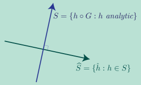
Figure 4: Orthogonality of two function classes: 1. Analytic functions of the probing signal, and 2. Corresponding solutions to Poisson’s equation.

2.3 Implications to filter design

Filter design proceeds under the assumption that the state process is ultimately bounded, in the sense of (17), but we require something slightly stronger for the family of QSA ODEs with fixed gain:

$\alpha^{0}$-Ultimate Boundedness:  With $\alpha^{0}>0$ constant, the family of QSA ODE models is $\alpha^{0}$-ultimately bounded if there is a fixed constant $B$ such that for each $\alpha\in(0,\alpha^{0}]$, initial condition $\Uptheta_{0}=\theta$, and $\Phi_{0}=z$, there is a finite time $t_{0}=t_{0}(\theta,z,\alpha)$ such that (17) holds for (27). It is also assumed that $t_{0}$ is continuous on its domain.

Criteria for $\alpha^{0}$-ultimate boundedness are surveyed in Section 2.4—see Thm. 2.9.

Assumption (A4) will be put in place throughout the remainder of the paper:

(A4)  The family of QSA ODE models is $\alpha^{0}$-ultimately bounded, and the mean flow satisfies the following two conditions:

• The ODE ${\mathchoice{\genfrac{}{}{}{1}{d}{dt}}{\genfrac{}{}{}{1}{d}{dt}}{\genfrac{}{}{}{3}{d}{dt}}{\genfrac{}{}{}{3}{d}{dt}}}\upvartheta_{t}={\widebar{f}}(\upvartheta_{t})$ is globally asymptotically stable with unique equilibrium $\theta^{*}$.

• The matrix $A^{*}={\bar{A}}(\theta^{*})$ is Hurwitz.

Subject to $\alpha^{0}$-ultimate boundedness we obtain the following consequence of the P-mean flow representation: there are finite constants $B_{\ell}\leq B_{\ell}^{+}$, independent of $\alpha$, such that for each $\theta=\Uptheta_{0}\in\mathbb{R}^{d}$ and $\alpha\in(0,\alpha^{0}]$, the following first entrance time is finite:

$$T_{\ell}(\theta)=\min\{t\geq 0:\max_{z_{0}}\|\Uptheta_{t}-\theta^{*}\|\leq B_{\ell}\}$$ (47a)

where the maximum is over $\Phi_{0}=z_{0}$. Moreover, for $t\geq T_{\ell}$ the trajectory is constrained to the larger region: For each $\Psi_{0}=(\theta,\Phi_{0})$,

$$\|\Uptheta_{t}-\theta^{*}\|\leq B_{\ell}^{+}\,,\qquad t\geq T_{\ell}(\theta)$$ (47b)

The time $T_{\ell}(\theta)$ depends on $\alpha$, but the constants $B_{\ell}$, $B_{\ell}^{+}$ do not.

Thm. 2.9 contains a criterion for $\alpha^{0}$-ultimate boundedness in a strong form. From (59) it follows that we can construct $\alpha^{0}$, together with a function ${\bar{T}}^{0}_{\ell}$, satisfying

$$T^{\alpha}_{\ell}(\theta)\leq{\bar{T}}^{\alpha}_{\ell}(\theta)\mathbin{:=}\frac{\alpha^{0}}{\alpha}{\bar{T}}^{0}_{\ell}(\theta)\,,\qquad\textit{for all $\theta$ and all $0<\alpha\leq\alpha^{0}$.}$$

The matrix $A^{*}={\bar{A}}(\theta^{*})$ is invertible under (A4). In this case we define a new function ${\bar{Y}}\colon\mathbb{R}^{d}\to\mathbb{R}^{d}$ via

$${\bar{Y}}=[A^{*}]^{-1}\widebar{\Upupsilon}$$ (48)

along with the fixed vectors $\widebar{\Upupsilon}^{*}=\widebar{\Upupsilon}(\theta^{*})$ and ${\bar{Y}}^{*}=[A^{*}]^{-1}\widebar{\Upupsilon}^{*}$. This notation is used for approximations obtained in [26, 34] for vanishing gain algorithms.

Proposition 2.6.

If Assumptions (A1)–(A4) hold, then for each initial condition $\Psi_{0}=(\theta,z_{0})\in\Uppi$,

$${\mathchoice{\genfrac{}{}{}{1}{d}{dt}}{\genfrac{}{}{}{1}{d}{dt}}{\genfrac{}{}{}{3}{d}{dt}}{\genfrac{}{}{}{3}{d}{dt}}}\Uptheta_{t}=\alpha A^{*}\bigl{[}\Uptheta_{t}-\theta^{*}-\alpha{\bar{Y}}^{*}+{\cal W}_{t}\bigr{]}+O(\alpha^{3})\,,\qquad\textit{for all $t\geq T_{\ell}(\theta)$}$$ (49)

This linearization is useful only if the matrix $A^{*}={\bar{A}}(\theta^{*})$ is Hurwitz, which is why this assumption appears in (A4). Subject to this assumption, the approximation (49) strongly suggests that we apply linear filtering techniques to reduce volatility.

For reasons that will become clear in the proof of Thm. 2.7 that follows, a filter that obtains AAD of order $O(\alpha^{2})$ can be chosen to be of second order, with bandwidth approximately equal to $\alpha$. It must also have unity DC gain, which brings us to the following special form for the filtered estimates:

$$\tfrac{d^{2}}{dt^{2}}\Uptheta^{\text{\tiny\sf F}}_{t}+2\gamma\zeta\tfrac{d}{dt}\Uptheta^{\text{\tiny\sf F}}_{t}+\gamma^{2}\Uptheta^{\text{\tiny\sf F}}_{t}=\gamma^{2}\Uptheta_{t}$$ (50)

It is the unity gain that prevents us from eliminating the error inherited from $\widebar{\Upupsilon}$, illustrated using ${\bar{Y}}^{*}$ in Fig. 1.

If ${\bar{Y}}^{*}=0$, then the coefficients $\gamma$ and $\zeta$ can be designed to reduce AAD dramatically. Theory predicts that a first order filter is not effective in general.

In the following companion to Thm. 2.15 we consider the family of QSA ODEs with fixed gain $\alpha$, and let the natural frequency $\gamma$ scale with $\alpha$.

Theorem 2.7.

Consider the solution to the QSA ODE with fixed gain. For each $\alpha>0$, the filtered estimates are obtained using (50), in which the value of $\zeta\in(0,1)$ is fixed, and $\gamma=\eta\alpha$ with $\eta>0$ also fixed.

Subject to Assumptions (A1)–(A4), the following conclusions hold for $0<\alpha\leq\alpha^{0}$:

$$\|\Uptheta_{t}-\theta^{*}\| \leq O(\alpha)+o(1)$$ (51a)

$$\|\Uptheta^{\text{\tiny\sf F}}_{t}-\theta^{*}\| \leq O(\alpha\gamma+\alpha^{2})+O(\alpha\|\widebar{\Upupsilon}^{*}\|)+o(1)$$ (51b)

with $\widebar{\Upupsilon}^{*}=\widebar{\Upupsilon}(\theta^{*})$. Consequently, the AAD for $\Uptheta^{\text{\tiny\sf F}}$ is bounded by $O(\alpha^{2})$ provided $\widebar{\Upupsilon}^{*}=0$.

The full proof is postponed to Section A.4. The proof of (51a) follows from two conclusions from the given assumptions: that the ODE (4) is exponentially asymptotically stable, by Prop. 2.10, which implies the existence of a smooth Lyapunov function for the mean flow. One solution is

$$V(\theta)=\int_{0}^{T}e^{\delta_{0}t}\|\upvartheta_{t}-\theta^{*}\|^{2}\,dt\,,\qquad\upvartheta_{0}=\theta\in\mathbb{R}^{d}$$ (52)

with $\delta_{0}>0$ chosen so that the integrand is vanishing, and $T>0$ sufficiently large so that $e^{\delta_{0}T}\|\upvartheta_{T}-\theta^{*}\|\leq{\mathchoice{\genfrac{}{}{}{1}{1}{2}}{\genfrac{}{}{}{1}{1}{2}}{\genfrac{}{}{}{3}{1}{2}}{\genfrac{}{}{}{3}{1}{2}}}\|\theta-\theta^{*}\|$ for any $\theta$. This Lyapunov function is then applied to the representation (43a). The proof of (51b) is then simpler since we can apply (51a) to justify linearization around $\theta^{*}$, applying an entirely linear systems theory analysis.

The approximations (2.7) imply bounds on the absolute deviation of parameter estimates, and hence the AAD. Bounds on bias and variance also follow as corollaries to Thm. 2.7.

Corollary 2.8.

Under the assumptions of Thm. 2.7,

• The asymptotic bias and variance (13) admit the bounds,

  $$\beta_{\Uptheta} =O(\alpha)\,,\quad\sigma^{2}_{\Uptheta}=O(\alpha^{2})\,,$$ (53a)

  $$\beta_{\Uptheta^{\text{\tiny\sf F}}} =O(\alpha)\,,\quad\sigma^{2}_{\Uptheta^{\text{\tiny\sf F}}}=O(\alpha^{2})\,,$$ (53b)

• If in addition (A0) holds, then

  $$\beta_{\Uptheta} =O(\alpha^{2})\,,\quad\sigma^{2}_{\Uptheta}=O(\alpha^{2})\,,$$ (53c)

  $$\beta_{\Uptheta^{\text{\tiny\sf F}}} =O(\alpha^{2})\,,\quad\sigma^{2}_{\Uptheta^{\text{\tiny\sf F}}}=O(\alpha^{4})\,.$$ (53d)

$\sqcap$$\sqcup$

Assumption (A0) has the largest impact on bias and variance. Equation (53c) tells us that the variance is of order $O(\alpha^{2})$ subject to this restriction on frequencies, which is remarkable when compared with standard results from SA theory (see (106) and discussion that follows). Filtering brings the variance down to $O(\alpha^{4})$; a restatement of the second bound in (53d).

Example

Two linear QSA ODEs will be used to illustrate the impact of $\widebar{\Upupsilon}^{*}$ on AAD:

$${\mathchoice{\genfrac{}{}{}{1}{d}{dt}}{\genfrac{}{}{}{1}{d}{dt}}{\genfrac{}{}{}{3}{d}{dt}}{\genfrac{}{}{}{3}{d}{dt}}}\Uptheta_{t} =\alpha[A_{t}\Uptheta_{t}+2\sin(\omega t)+1]$$ (54a)

$${\mathchoice{\genfrac{}{}{}{1}{d}{dt}}{\genfrac{}{}{}{1}{d}{dt}}{\genfrac{}{}{}{3}{d}{dt}}{\genfrac{}{}{}{3}{d}{dt}}}\Uptheta_{t} =\alpha[A_{t}\Uptheta_{t}+2\cos(\omega t)+1]$$ (54b)

where $A_{t}=-(1+\sin(\omega t))$ with $\omega>0$. Assumption (A0b) holds for (54a) with $K=1$ in (7), using ${\scalebox{1.1}{$\upxi$}}^{0}_{t}=\cos(\omega t)$. In the second case (54b), Assumption (A0b) is violated: any realization of ${\scalebox{1.1}{$\upxi$}}^{0}_{t}$ will require $K=2$ with $\omega_{1}=\omega_{2}$.

We obtain a formula for $\widebar{\Upupsilon}^{*}$ in each case, based on the following observations:

• They share the common mean vector field ${\widebar{f}}(\theta)=-\theta+1$, so that $\theta^{*}=1$.

• They also share the same linearizations: $A(\theta,{\scalebox{1.1}{$\upxi$}})=\partial_{\theta}f(\theta,{\scalebox{1.1}{$\upxi$}})=-(1+\sin(\omega t))$ and $A^{*}=-1$.

  Consequently, ${\bar{Y}}(\theta)=[A^{*}]^{-1}\widebar{\Upupsilon}(\theta)=-\widebar{\Upupsilon}(\theta)$, and for any $\theta$ and $t$,

  $$\widehat{A}(\theta,\Phi_{t})=-\omega^{-1}\cos(\omega t)$$

  Observe that $\int\widehat{A}(\theta,z)\,\uppi(dz)={\mathchoice{{\mathchoice{\mbox{\large\sf 0}}{\mbox{\large\sf 0}}{\mbox{\tiny\sf 0}}{\mbox{\tiny\sf 0}}}}{\mbox{\sf 0}}{\mbox{\tiny\sf 0}}{\mbox{\tiny\sf 0}}}$ and ${\mathchoice{\genfrac{}{}{}{1}{d}{dt}}{\genfrac{}{}{}{1}{d}{dt}}{\genfrac{}{}{}{3}{d}{dt}}{\genfrac{}{}{}{3}{d}{dt}}}\widehat{A}(\theta,\Phi_{t})=-[A(\theta,{\scalebox{1.1}{$\upxi$}}_{t})-{\bar{A}}(\theta)]$, as required.

• A crucial difference is the steady-state apparent noise: $f(\theta^{*},{\scalebox{1.1}{$\upxi$}}_{t})=\sin(\omega t)$ for (54a), and $f(\theta^{*},{\scalebox{1.1}{$\upxi$}}_{t})=-\sin(\omega t)+2\cos(\omega t)$ for (54b).

From the (34e) we find that $\widebar{\Upupsilon}(\theta)=\widebar{\Upupsilon}^{*}$ (independent of $\theta$):

$$-{\bar{Y}}(\theta)=\widebar{\Upupsilon}(\theta) \mathbin{:=}-\lim_{T\to\infty}\frac{1}{T}\int_{0}^{T}\widehat{A}(\theta,\Phi_{t})\cdot f(\theta,{\scalebox{1.1}{$\upxi$}}_{t})\,dt$$

$$=\begin{cases}\displaystyle\ \ \ 0&\text{Model \eqref{e:lin_barY0}}\\ \displaystyle\ \ -\lim_{T\to\infty}\frac{1}{T}\int_{0}^{T}\{-\omega^{-1}\cos(\omega t)\}\cdot\{2\cos(\omega t)\}\,dt=\frac{1}{\omega}\quad&\text{Model \eqref{e:lin_barYnot}}\end{cases}$$

In each case, we have used the fact that $\widehat{A}(\theta,\Phi_{t})$ and $\widehat{A}(\theta,\Phi_{t})\cdot\sin(\omega t)$ each have time average equal to zero.

Simulation Setup  We are interested in comparing AAD for $\bm{\Uptheta}$ with and without filtering. The special case $\omega=0.1$ was considered, many gains were tested in the range $\alpha\in[10^{-3},0.9]$, and in each experiment the solution to the QSA ODE was approximated using an Euler scheme with sampling time of $0.1$ sec.

Data $\{\Uptheta_{t}\}$ for each choice of $\alpha$ was then used to obtain the two filtered estimates:

$${\Uptheta}^{1\text{\tiny\sf F}}_{t}=\int^{t}_{0}h^{1}_{t-\tau}\Uptheta_{\tau}\,d\tau,\qquad{\Uptheta}^{2\text{\tiny\sf F}}_{t}=\int^{t}_{0}h^{2}_{t-\tau}\Uptheta_{\tau}\,d\tau$$

where $h^{1}_{t}$ and $h^{2}_{t}$ have Laplace transforms:

$$H_{1}(s)=\frac{\gamma}{s+\gamma},\qquad H_{2}(s)=\frac{\gamma^{2}}{s^{2}+2\zeta\gamma s+\gamma^{2}}\,,\qquad\textit{ with $\gamma=\alpha$, $\zeta=0.8$. }$$ (55)

The steady-state $L_{1}$ norm of the error was approximated using the Monte-Carlo estimate,

$$\|\Uptheta_{\alpha}\|_{L_{1}}\mathbin{:=}\frac{1}{T-T_{0}}\int^{T}_{T_{0}}|\Uptheta_{\tau}-\theta^{*}|\,d\tau$$

taking $T_{0}=0.8T$, so that only the final $20\%$ of the run was included. This was repeated to obtain $\|{\Uptheta}^{1\text{\tiny\sf F}}_{\alpha}\|_{L_{1}}$ and $\|{\Uptheta}^{2\text{\tiny\sf F}}_{\alpha}\|_{L_{1}}$ for each value of $\alpha$ considered.

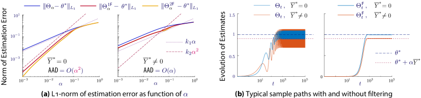
Figure 5: AAD as a function of $\alpha$ for different filtering techniques (left). Impact of ${\bar{Y}}^{*}$ on estimation error (right).

Results  The final estimates for each case are shown plotted against $\alpha$ on a logarithmic scale in Fig. 5 (a). Also shown for comparison with expected bounds are plots of the linear functions $r_{1}(\alpha)=k_{1}\alpha$, $r_{2}(\alpha)=k_{2}\alpha^{2}$. The constants $k_{1},k_{2}$ were chosen to aid comparison. The results agree with Thm. 2.7. In particular, we see in Fig. 5 that the term $\alpha{\bar{Y}}^{*}$ dominates the estimation error when ${\bar{Y}}^{*}\neq 0$. In this case, filtering has no improvement on reducing AAD of order $O(\alpha)$. When ${\bar{Y}}^{*}=0$, Fig. 5 (a) shows that filtering reduces AAD to $O(\alpha^{2})$ for $\alpha<0.1$, and this is observed for both first and second order low pass filters. An explanation for the similar performance is contained in Section A.3.

The evolution of the process $\{{\Uptheta}^{2\text{\tiny\sf F}}_{t}\}$ for the specific case of $\alpha=0.01$ is shown in Fig. 5 (b). The volatility of $\bm{\Uptheta}$ is massive in each case, and reduced dramatically with filtering.

These results illustrate the importance of carefully designing the probing signal: the inclusion of a phase shift in one of the entries of $\bm{\upxi}$ might appear harmless. In fact, this small change results in significant estimation error—10% in this example.

2.4 Some stability theory

Here we establish ultimate boundedness of the QSA ODE under either of the two stability criteria surveyed in the introduction. The Lyapunov bound is recalled here in slightly modified form, and given a new name:

• There exists a $C^{1}$ function $V:\mathbb{R}^{d}\rightarrow[1,\infty)$ and a constant $\delta_{0}>0$ such that the following bound holds for (4) for any time $\tau\geq 0$ for which $\|\upvartheta_{\tau}\|\geq\delta_{0}^{-1}$:

  $$\frac{d}{d\tau}V(\upvartheta_{\tau})\leq-\delta_{0}V(\upvartheta_{\tau})$$ (56)

  Moreover, the function is Lipschitz continuous with linear growth: there exists a constant $L_{V}<\infty$ such that

  $$|V(\theta^{\prime})-V(\theta)| \leq L_{V}\|\theta^{\prime}-\theta\|\,, \theta \theta^{\prime}$$ for all , . (57)

  $$V(\theta) \geq\|\theta\|\,, \|\theta\|\geq\delta_{0}^{-1}$$ when

The use of “(V4)” is because of its close connection with a similar “drift condition” in the theory of Markov chains and processes [35].

It is convenient to consider a relaxation:

• There is a function $V\colon\mathbb{R}^{d}\to\mathbb{R}_{+}$ satisfying the bound (57), together with constants $T<\infty$ and $\delta_{1}>0$ such that for each initial condition $\upvartheta_{0}$ and $\tau\geq 0$,

  $$V(\upvartheta_{\tau+T})-V(\upvartheta_{\tau})\leq-\delta_{1}\|\upvartheta_{\tau}\|,\quad\text{for all }\tau\geq 0\,,\ \|\upvartheta_{\tau}\|>\delta_{1}^{-1}$$ (58)

This unifies the theory since it is obviously implied by (V4), and we will see that it is implied by asymptotic stability of the ODE@$\infty$.

Theorem 2.9.

Suppose that (A1) and the Lyapunov bound (V4’) hold for the fixed gain QSA ODE (27). Then, there is $\alpha^{0}>0$ and positive constants $b$ and $\delta$ such that the following bounds hold for any $\alpha\in(0,\alpha^{0}]$ and any initial condition $\Uptheta_{0},\Phi_{0}$:

$$\|\Uptheta_{t}\|\leq b\|\Uptheta_{0}\|\exp(-\alpha\delta t)\,,\quad\textit{for $t\leq T_{1}$, where $T_{1}=\min\{t:\|\Uptheta_{t}\|\leq\delta^{-1}\}$.}$$ (59)

Consequently, the family of QSA ODE models is $\alpha^{0}$-ultimately bounded.

The full proof of the theorem is postponed to the Appendix, based on the following two steps:

• Bounds on the difference between solutions to QSA ODE (27) and the solutions to the ODE,

  $${\mathchoice{\genfrac{}{}{}{1}{d}{dt}}{\genfrac{}{}{}{1}{d}{dt}}{\genfrac{}{}{}{3}{d}{dt}}{\genfrac{}{}{}{3}{d}{dt}}}\upvartheta_{t}=\alpha{\widebar{f}}(\upvartheta_{t})$$ (60)

• A proof that (V4’) implies a version of (59) for the mean flow.

A similar result is established in [26] for the QSA ODE with vanishing gain.

The implications of (V4’) for the mean flow are summarized here:

Proposition 2.10.

Suppose that (V4’) holds, along with (A1) and (A4). Then the ODE (4) is exponentially asymptotically stable: for positive constants $b$ and $\delta$, and any initial condition $\upvartheta_{0}$,

$$\|\upvartheta_{t}-\theta^{*}\|\leq b\|\upvartheta_{0}-\theta^{*}\|e^{-\delta t}\,,\qquad t\geq 0$$

Proof.

The proof is obtained by interpreting Fig. 6. The time $T_{1}$ is the first $t\geq 0$ such that $\upvartheta_{t}\in B_{1}$, and $T_{2}$ the first $t\geq T_{1}$ such that $\upvartheta_{t}\in B_{2}$. The set $B_{1}$ is defined in the figure, and $B_{2}$ is a region of exponential asymptotic stability.

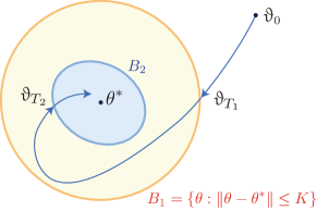
Figure 6: Roadmap for the proof of exponential asymptotic stability for ${\mathchoice{\genfrac{}{}{}{1}{d}{dt}}{\genfrac{}{}{}{1}{d}{dt}}{\genfrac{}{}{}{3}{d}{dt}}{\genfrac{}{}{}{3}{d}{dt}}}\upvartheta_{t}={\widebar{f}}(\upvartheta_{t})$.

Lemma A.10 tells us that, under (V4’), the constant $$K B_{1} b_{1} \delta_{1} \upvartheta_{0}\in B_{1}^{c}$$ defining can be chosen sufficiently large so that there are positive constants and such that the following bound holds for :

$$\|\upvartheta_{T_{1}}-\theta^{*}\|\leq b_{1}\|\upvartheta_{0}-\theta^{*}\|e^{-\delta_{1}T_{1}}$$ (61a)

The set $$B_{1} T_{2}-T_{1} \upvartheta_{0} b_{1}$$ is bounded, so that is uniformly bounded over all initial conditions for —this is where we apply globally asymptotically stability from (A4). Consequently, the constant can be increased if necessary to obtain

$$\|\upvartheta_{T_{2}}-\theta^{*}\|\leq b_{1}\|\upvartheta_{T_{1}}-\theta^{*}\|$$ (61b)

Finally we specify $$B_{2} \upvartheta_{t}\in B_{2} t\geq T_{2} b_{2} \delta_{2}$$: it is chosen so that it is absorbing, that is for all , and for some positive constants and ,

$$\|\upvartheta_{t}-\theta^{*}\|\leq b_{2}\|\upvartheta_{T_{2}}-\theta^{*}\|e^{-\delta_{2}(t-T_{2})}\,,\qquad t\geq T_{2}.$$ (61c)

The proof is completed on combining the three bounds (61c), with $$\delta=\min(\delta_{1},\delta_{2})$$.

$\sqcap$$\sqcup$

2.4.1 QSA solidarity

Here we establish bounds between the solutions of the QSA ODE and the mean flow (60). However, it is convenient to eliminate the $\alpha$ in (60) through a change of time-scale: If $\bm{\upvartheta}$ is a solution to (60), then $\{\upvartheta_{t/\alpha}:t\geq 0\}$ is a solution to (4).

Similarly, on denoting $\Uptheta_{t}^{\alpha}=\Uptheta_{t/\alpha}$, the scaling is removed from (27):

$${\mathchoice{\genfrac{}{}{}{1}{d}{dt}}{\genfrac{}{}{}{1}{d}{dt}}{\genfrac{}{}{}{3}{d}{dt}}{\genfrac{}{}{}{3}{d}{dt}}}\Uptheta^{\alpha}_{t}=f(\Uptheta^{\alpha}_{t},{\scalebox{1.1}{$\upxi$}}^{\alpha}_{t})$$ (62)

with ${\scalebox{1.1}{$\upxi$}}^{\alpha}_{t}\mathbin{:=}{\scalebox{1.1}{$\upxi$}}_{t/\alpha}$. Hence time is speeded up for the probing signal when $\alpha>0$ is small.

Proposition 2.11.

Consider the QSA ODE subject to (A1). There is $\alpha^{0}>0$, $B_{0}<\infty$, and $\varepsilon_{0}\colon\mathbb{R}_{+}\to\mathbb{R}_{+}$ such that the following uniform bounds hold for respective solutions to (62) and (4), with common initial condition $\Uptheta_{0}=\upvartheta_{0}=\theta_{0}\in\mathbb{R}^{d}$. For each $\Phi_{0}\in\Upomega$, $T>0$, and $\alpha\in(0,\alpha^{0}]$:

$$\|\Uptheta_{T}^{\alpha}-\upvartheta_{T}\|\leq B_{0}\exp(2L_{f}T)\bigl{[}1+\|\theta_{0}\|\bigr{]}\varepsilon_{0}(\alpha)$$ (63)

with $\varepsilon_{0}(\alpha)\to 0$ as $\alpha\downarrow 0$.

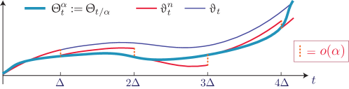
Figure 7: Solidarity between the time-scaled QSA ODE and the mean flow.

The proof of the proposition is contained in the Appendix. The main idea is illustrated in Fig. 7: the time axis is partitioned into intervals of width $\Delta>0$ on which $\Uptheta_{t}^{\alpha}$ is approximately constant. With $\tau_{n}=n\Delta$, we let $\{\upvartheta^{n}_{t}:t\geq\tau_{n}\}$ denote the solution to (4) with $\upvartheta^{n}_{\tau_{n}}=\Uptheta^{\alpha}_{\tau_{n}}$. The proof follows in three steps: 1.  bounds on the error $\|\upvartheta^{n}_{t}-\Uptheta^{\alpha}_{t}\|$ for $t\in[\tau_{n},\tau_{n+1}]$; 2.  bounds on $\|\upvartheta^{n}_{t}-\upvartheta_{t}\|$ for all $t$ and $n$, and 3.  combine 1 and 2 (with minor additional approximations) to complete the proof.

2.4.2 ODE@$\infty$

We now explain how to establish (V4’) based on the ODE@$\infty$ introduced in Section 1.3, with vector field ${\widebar{f}}_{\infty}$ defined in (19). The limit exists in many applications, and is often much simpler than ${\widebar{f}}$. In particular, ${\widebar{f}}_{\infty}(0)=0$ (the origin is a stationary point), and the function is radially linear: ${\widebar{f}}_{\infty}(c\theta)=c{\widebar{f}}_{\infty}(\theta)$ for any $\theta\in\mathbb{R}^{d}$ and $c\geq 0$. Based on these properties it is known that the origin is locally stable in the sense of Lyapunov if and only if it is globally exponentially asymptotically stable [8].

The following result follows from arguments leading to the proof of [34, Prop. 4.22]:

Theorem 2.12.

Suppose that the limit (19) exists, and suppose that the origin is asymptotically stable for the ODE@$\infty$. Then, there is a Lipschitz continuous solution to (58).     $\sqcap$$\sqcup$

The proof of the theorem is contained in the Appendix, where it is shown that the following function is a solution to (58), similar to (52):

$$V(\theta)=\int_{0}^{T}\|\upvartheta_{t}^{\infty}\|\,dt\,,\qquad\upvartheta_{0}^{\infty}=\theta\in\mathbb{R}^{d}$$ (64)

Lipschitz continuity of both ${\widebar{f}}_{\infty}$ and $V$ is inherited from ${\widebar{f}}$.

To illustrate application of the theorem, consider the gradient flow for which ${\widebar{f}}=-\nabla\Upgamma$:

$${\mathchoice{\genfrac{}{}{}{1}{d}{dt}}{\genfrac{}{}{}{1}{d}{dt}}{\genfrac{}{}{}{3}{d}{dt}}{\genfrac{}{}{}{3}{d}{dt}}}\upvartheta=-\nabla\Upgamma\,(\upvartheta)$$ (65)

with $\Upgamma\colon\mathbb{R}^{d}\to\mathbb{R}$, with minimum denoted $\Upgamma^{\text{\tiny\sf opt}}$. The existence of ${\widebar{f}}_{\infty}$ implies that the following limit also holds:

$$\Upgamma_{\infty}(\theta)\mathbin{:=}\lim_{r\to\infty}r^{-2}\Upgamma(r\theta)\,,\qquad\theta\in\mathbb{R}^{d}$$ (66)

This follows from the representation

$$\Upgamma(\theta)-\Upgamma(0)=\int_{0}^{1}{\mathchoice{\genfrac{}{}{}{1}{d}{dt}}{\genfrac{}{}{}{1}{d}{dt}}{\genfrac{}{}{}{3}{d}{dt}}{\genfrac{}{}{}{3}{d}{dt}}}\Upgamma(t\theta)\,dt=\int_{0}^{1}\theta^{\intercal}\nabla\Upgamma\,(t\theta)\,dt$$

which implies the representation ${\widebar{f}}_{\infty}(\theta)=-\nabla\Upgamma_{\infty}(\theta)$ and

$$\Upgamma_{\infty}(\theta)=-\int_{0}^{1}\theta^{\intercal}\nabla\Upgamma_{\infty}(t\theta)\,dt\,,\qquad\theta\in\mathbb{R}^{d}$$ (67)

The gradient flow is ultimately bounded under mild assumptions:

Proposition 2.13.

Suppose that $\Upgamma_{\infty}$ is $C^{1}$, and $\Upgamma_{\infty}(\theta)>0$ for $\theta\neq 0$. Then the ODE@$\infty$ for the gradient flow is exponentially asymptotically stable: for some $B<\infty$, $\delta>0$, and any initial $\upvartheta^{\infty}_{0}\in\mathbb{R}^{d}$,

$$\|\upvartheta^{\infty}_{t}\|^{2}\leq B\|\upvartheta^{\infty}_{0}\|^{2}e^{-\delta t}\,,\qquad\textit{for $t\geq 0$.}$$ (68)

Consequently, the gradient flow itself is ultimately bounded.

Proof.

Both $\Upgamma_{\infty}$ and $\|\nabla\Upgamma_{\infty}\|^{2}$ are bounded above and below by quadratic functions—this follows from continuity and the radial homogeneity properties

$$\Upgamma_{\infty}(r\theta)=r^{2}\Upgamma_{\infty}(\theta)\,,\qquad\nabla\Upgamma_{\infty}\,(r\theta)=r\nabla\Upgamma_{\infty}\,(\theta)\,,\qquad\theta\in\mathbb{R}^{d}\,,\ r>0$$

Hence the following constants exist as finite positive numbers,

$$\kappa_{+}=\max\frac{\Upgamma_{\infty}(\theta)}{\|\theta\|^{2}}\,,\quad\kappa_{-}=\min\frac{\Upgamma_{\infty}(\theta)}{\|\theta\|^{2}}\,,\qquad\chi_{+}=\max\frac{\|\nabla\Upgamma_{\infty}\,(\theta)\|^{2}}{\|\theta\|^{2}}\,,\quad\chi_{-}=\min\frac{\|\nabla\Upgamma_{\infty}\,(\theta)\|^{2}}{\|\theta\|^{2}}\,,$$

where the min and max are over non-zero $\theta\in\mathbb{R}^{d}$.

We have ${\mathchoice{\genfrac{}{}{}{1}{d}{dt}}{\genfrac{}{}{}{1}{d}{dt}}{\genfrac{}{}{}{3}{d}{dt}}{\genfrac{}{}{}{3}{d}{dt}}}\Upgamma_{\infty}(\upvartheta^{\infty})=-\|\nabla\Upgamma_{\infty}\,(\upvartheta^{\infty})\|^{2}$, and from the above definitions we conclude that ${\mathchoice{\genfrac{}{}{}{1}{d}{dt}}{\genfrac{}{}{}{1}{d}{dt}}{\genfrac{}{}{}{3}{d}{dt}}{\genfrac{}{}{}{3}{d}{dt}}}\Upgamma_{\infty}(\upvartheta^{\infty})=-\delta\Upgamma_{\infty}(\upvartheta^{\infty})$ with $\delta=\chi_{-}/\kappa_{+}$. Hence $\Upgamma_{\infty}(\upvartheta^{\infty}_{t})\leq e^{-\delta t}\Upgamma_{\infty}(\upvartheta^{\infty}_{0})$, which completes the proof using $B=\kappa_{+}/{\kappa_{-}}$.     $\sqcap$$\sqcup$

2.5 Extensions

Three extensions follow.

• The first is to almost periodic linear systems to illustrate the connections, and because one conclusion is useful in establishing finer bounds for general QSA ODEs.

• Then, we review the main conclusions from [26] for vanishing gain QSA.

• Finally, we explain how bias bounds extend to stochastic approximation.

2.5.1 Almost periodic linear systems

A quasi periodic linear system is a special case of QSA with constant gain:

$${\mathchoice{\genfrac{}{}{}{1}{d}{dt}}{\genfrac{}{}{}{1}{d}{dt}}{\genfrac{}{}{}{3}{d}{dt}}{\genfrac{}{}{}{3}{d}{dt}}}\Uptheta_{t}=\alpha A_{t}\Uptheta_{t}\,,\qquad A_{t}\mathbin{:=}A({\scalebox{1.1}{$\upxi$}}_{t})\,,$$ (69)

The matrix-valued function of time $D_{T}=\int_{0}^{T}A_{t}\,dt$, $T\geq 0$, emerges in the theory. In the notation of Prop. 2.14 this becomes $D_{T}=T{\bar{A}}^{*}+\widehat{A}_{0}-\widehat{A}_{T}$. If $A_{T}$ and $D_{T}$ commute for each $T$, one obtains a simple expression for the state transition matrix [30, 52].

In this linear case, a bound on the Lyapunov exponent is equivalent to a bound on the following for each non-zero initial condition $\theta$:

$$\Lambda_{\Uptheta}(\theta)=\lim_{t\to\infty}\tfrac{1}{t}\log(\|\Uptheta_{t}\|)\,,\qquad\Uptheta_{0}=\theta\in\mathbb{R}^{d}$$ (70)

Proposition 2.14 (Application to Quasi Periodic Linear Systems).

Consider the linear QSA ODE (69), subject to the following subset of Assumptions (A1)–(A4):

• $A^{*}\mathbin{:=}{\sf E}[A({\scalebox{1.1}{$\upxi$}})]$ is Hurwitz.

• ${\hat{f}}(\theta,z)=\widehat{A}(z)\theta$, which solves

  $$\widehat{A}(\Phi_{t_{0}})=\int_{t_{0}}^{t_{1}}[A({\scalebox{1.1}{$\upxi$}}_{t})-A(\theta)]\,dt+\widehat{A}(\Phi_{t_{1}})\,,\qquad 0\leq t_{0}\leq t_{1}$$

For each $\alpha>0$, let $\Lambda_{\Uptheta}^{\alpha}$ denote the Lyapunov exponent associated with (69). Then $\Lambda_{\Uptheta}^{\alpha}<0$ for sufficiently small $\alpha>0$, and

$$\lim_{\alpha\downarrow 0}\frac{1}{\alpha}\Lambda_{\Uptheta}^{\alpha}=\text{\rm Re}(\lambda_{1})<0$$ (71)

where $\lambda_{1}$ is an eigenvalue of $A^{*}$ with maximal real part.

Proof.

We establish only the upper bound,

$$\mathop{\rm lim{\,}sup}_{\alpha\downarrow 0}\frac{1}{\alpha}\Lambda_{\Uptheta}^{\alpha}\leq\text{Re}(\lambda_{1})$$ (72)

leaving the technical details for the lower bound to the reader.

The following calculation is identical to the first step in the proof of Thm. 2.3, using the shorthand $\widehat{A}_{t}=\widehat{A}(\Phi_{t})$:

$${\mathchoice{\genfrac{}{}{}{1}{d}{dt}}{\genfrac{}{}{}{1}{d}{dt}}{\genfrac{}{}{}{3}{d}{dt}}{\genfrac{}{}{}{3}{d}{dt}}}{\hat{f}}(\Uptheta_{t},\Phi_{t})\mathbin{:=}{\mathchoice{\genfrac{}{}{}{1}{d}{dt}}{\genfrac{}{}{}{1}{d}{dt}}{\genfrac{}{}{}{3}{d}{dt}}{\genfrac{}{}{}{3}{d}{dt}}}\bigl{(}\widehat{A}_{t}\Uptheta_{t}\bigr{)} =\bigl{(}{\mathchoice{\genfrac{}{}{}{1}{d}{dt}}{\genfrac{}{}{}{1}{d}{dt}}{\genfrac{}{}{}{3}{d}{dt}}{\genfrac{}{}{}{3}{d}{dt}}}\widehat{A}_{t}\bigr{)}\Uptheta_{t}+\widehat{A}_{t}\bigl{(}{\mathchoice{\genfrac{}{}{}{1}{d}{dt}}{\genfrac{}{}{}{1}{d}{dt}}{\genfrac{}{}{}{3}{d}{dt}}{\genfrac{}{}{}{3}{d}{dt}}}\Uptheta_{t}\bigr{)}$$

$$=-[A_{t}-A^{*}]\Uptheta_{t}+\alpha\widehat{A}_{t}A_{t}\Uptheta_{t}$$

Note that $\Upupsilon_{t}\mathbin{:=}-\widehat{A}_{t}A_{t}\Uptheta_{t}$ in the notation of Thm. 2.3.

The resulting identity $A_{t}\Uptheta_{t}=A^{*}+\alpha\widehat{A}_{t}A_{t}-{\mathchoice{\genfrac{}{}{}{1}{d}{dt}}{\genfrac{}{}{}{1}{d}{dt}}{\genfrac{}{}{}{3}{d}{dt}}{\genfrac{}{}{}{3}{d}{dt}}}\bigl{(}\widehat{A}_{t}\Uptheta_{t}\bigr{)}$ is substituted into (69) to obtain

$${\mathchoice{\genfrac{}{}{}{1}{d}{dt}}{\genfrac{}{}{}{1}{d}{dt}}{\genfrac{}{}{}{3}{d}{dt}}{\genfrac{}{}{}{3}{d}{dt}}}\Uptheta_{t}=\alpha\bigl{[}A^{*}+\alpha\widehat{A}_{t}A_{t}\bigr{]}\Uptheta_{t}-\alpha{\mathchoice{\genfrac{}{}{}{1}{d}{dt}}{\genfrac{}{}{}{1}{d}{dt}}{\genfrac{}{}{}{3}{d}{dt}}{\genfrac{}{}{}{3}{d}{dt}}}\bigl{(}\widehat{A}_{t}\Uptheta_{t}\bigr{)}$$

This motivates the introduction of a new state variable $Y_{t}=[I+\alpha\widehat{A}_{t}]\Uptheta_{t}$ to obtain the state space model

$${\mathchoice{\genfrac{}{}{}{1}{d}{dt}}{\genfrac{}{}{}{1}{d}{dt}}{\genfrac{}{}{}{3}{d}{dt}}{\genfrac{}{}{}{3}{d}{dt}}}Y_{t}=\alpha\bigl{[}A^{*}+\alpha\widehat{A}_{t}A_{t}\bigr{]}\bigl{[}I+\alpha\widehat{A}_{t}\bigr{]}^{-1}Y_{t}$$

The inverse exists for all sufficiently small $\alpha>0$ since $\{\widehat{A}_{t}\}$ is bounded, from which we obtain

$${\mathchoice{\genfrac{}{}{}{1}{d}{dt}}{\genfrac{}{}{}{1}{d}{dt}}{\genfrac{}{}{}{3}{d}{dt}}{\genfrac{}{}{}{3}{d}{dt}}}Y_{t}=\alpha\bigl{[}A^{*}+\alpha{\cal E}^{\alpha}_{t}\bigr{]}Y_{t}$$ (73)

in which $\{{\cal E}^{\alpha}_{t}\}$ is uniformly bounded in $t$, and $\alpha$ in a neighborhood of the origin. For each $t$,

$$\lim_{\alpha\downarrow 0}\tfrac{1}{\alpha}{\cal E}^{\alpha}_{t}=\widehat{A}_{t}A_{t}-A^{*}\widehat{A}_{t}$$

The remainder of the proof is standard. First, for any positive definite matrix $P$, on taking $V(\theta)=\theta^{\intercal}P\theta$ we have

$$2\Lambda_{\Uptheta}(\theta)=\lim_{t\to\infty}\tfrac{1}{t}\log(V(\Uptheta_{t}))=\lim_{t\to\infty}\tfrac{1}{t}\log(V(Y_{t}))$$

This is simply a consequence of the fact that all norms are equivalent on $\mathbb{R}^{d}$, along with uniform bounds on the norm of $[I+\alpha\widehat{A}_{t}]$ and its inverse.

The matrix $\delta I+A^{*}$ is Hurwitz for any $0\leq\delta<|\text{Re}(\lambda_{1})|$, so that there is a solution $P>0$ to the Lyapunov equation ${A^{*}}^{\intercal}P+PA^{*}+2\delta P=-I$. Applying (73) gives

$${\mathchoice{\genfrac{}{}{}{1}{d}{dt}}{\genfrac{}{}{}{1}{d}{dt}}{\genfrac{}{}{}{3}{d}{dt}}{\genfrac{}{}{}{3}{d}{dt}}}V(Y_{t})=-\alpha\bigl{[}2\delta V(Y_{t})+\|Y_{t}\|^{2}\bigr{]}+\alpha^{2}Y_{t}^{\intercal}\bigl{[}{{\cal E}^{\alpha}_{t}}^{\intercal}P+P{\cal E}^{\alpha}_{t}\bigr{]}Y_{t}.$$

For $\alpha>0$ sufficiently small we obtain the upper bound,

$$2\Lambda_{\Uptheta}(\theta)=\lim_{t\to\infty}\tfrac{1}{t}\log(V(Y_{t})) \leq-2\alpha\delta+O(\alpha^{2})$$

$$\textit{giving}\quad\mathop{\rm lim{\,}sup}_{\alpha\downarrow 0}\frac{1}{\alpha}\Lambda_{\Uptheta}^{\alpha} \leq-\delta$$

This establishes (72) since $\delta<|\text{Re}(\lambda_{1})|$ is arbitrary.     $\sqcap$$\sqcup$

The representation (73) suggests that we might go further, using repeated applications of Poisson’s equation as in our treatment of general QSA ODEs. On writing

$${\mathchoice{\genfrac{}{}{}{1}{d}{dt}}{\genfrac{}{}{}{1}{d}{dt}}{\genfrac{}{}{}{3}{d}{dt}}{\genfrac{}{}{}{3}{d}{dt}}}Y_{t}=\alpha A_{t}^{1}Y_{t}\,,\qquad A_{t}^{1}=A^{*}+\alpha{\cal E}^{\alpha}_{t}$$

successive applications of this approach would lead to a family of almost periodic linear systems,

$${\mathchoice{\genfrac{}{}{}{1}{d}{dt}}{\genfrac{}{}{}{1}{d}{dt}}{\genfrac{}{}{}{3}{d}{dt}}{\genfrac{}{}{}{3}{d}{dt}}}Y_{t}^{i}=\alpha A_{t}^{i}Y_{t}^{i}\,,\qquad i\geq 2$$

The hope is that we would obtain $A_{t}^{i}\to A^{*}$ as $i\to\infty$ for each $t$, leading to the time-homogeneous linear system, combined with time varying coordinate transformation $\mathcal{T}_{t}$:

$${\mathchoice{\genfrac{}{}{}{1}{d}{dt}}{\genfrac{}{}{}{1}{d}{dt}}{\genfrac{}{}{}{3}{d}{dt}}{\genfrac{}{}{}{3}{d}{dt}}}Y_{t}^{\infty}=A^{*}Y_{t}^{\infty}\,,\qquad\Uptheta_{t}=\mathcal{T}_{t}Y_{t}^{\infty}$$

2.5.2 Vanishing gain

The main result of [26], concerns rates of convergence for the QSA ODE, and averaging techniques to improve these rates. The gain is taken of the form (6) with $\rho\in({\mathchoice{\genfrac{}{}{}{1}{1}{2}}{\genfrac{}{}{}{1}{1}{2}}{\genfrac{}{}{}{3}{1}{2}}{\genfrac{}{}{}{3}{1}{2}}},1)$ and $t_{e}=1$. In this setting, the use of Polyak-Ruppert averaging is sometimes effective. At time $T$, the averaged parameter estimate is defined as

$$\Uptheta^{\text{\tiny\sf PR}}_{T}\mathbin{:=}\frac{1}{T-T_{0}}\int_{T_{0}}^{T}\Uptheta_{t}\,dt$$ (74)

in which the starting time scales linearly with $T$: for fixed $\kappa>1$ we chose $T_{0}$ to solve $1/(T-T_{0})=\kappa/T$.

Theorem 2.15.

Suppose that Assumptions (A1)–(A4) hold, and that the solutions to the QSA ODE (5) have bounded sample paths. Then the following conclusions hold:

$$\Uptheta_{t} =\theta^{*}-a_{t}{\hat{f}}^{*}_{t}+O(a_{t}\|{\bar{Y}}^{*}\|)+o(a_{t}) t\geq t_{0}$$ (75a)

$$\Uptheta^{\text{\tiny\sf PR}}_{T} =\theta^{*}+a_{T}[c(\kappa,\rho)+o(1)]{\bar{Y}}^{*}+O(T^{-2\rho})\,,\qquad T_{0}\geq t_{0}$$ (75b)

where $c(\kappa,\rho)=c(\kappa,\rho)=\kappa[1-(1-1/\kappa)^{1-\rho}]/(1-\rho)$, and ${\bar{Y}}^{*}=[A^{*}]^{-1}\widebar{\Upupsilon}^{*}$.

Consequently, $\Uptheta^{\text{\tiny\sf PR}}_{T}$ converges to $\theta^{*}$ with rate bounded by $O(T^{-2\rho})$ if and only if ${\bar{Y}}^{*}=0$.

This is a remarkable conclusion, since we can choose $\rho$ to obtain a rate of convergence arbitrarily close to $O(T^{-2})$.

The key step in the proof is to obtain a version of the perturbative mean flow, this time for the scaled error,

$$Z_{t}=\frac{1}{a_{t}}\bigl{(}\Uptheta_{t}-\theta^{*}\bigr{)}\,,\qquad t\geq t_{0}$$ (76)

The analysis is entirely local, so that a linearization around $\theta^{*}$ is justified:

$${\mathchoice{\genfrac{}{}{}{1}{d}{dt}}{\genfrac{}{}{}{1}{d}{dt}}{\genfrac{}{}{}{3}{d}{dt}}{\genfrac{}{}{}{3}{d}{dt}}}Z_{t}=a_{t}[o(1)I+A^{*}]Z_{t}+\widetilde{\Xi}_{t}$$

in which the definition of the apparent noise $\{\widetilde{\Xi}_{t}\}$ is unchanged. Applying (42) then gives,

$${\mathchoice{\genfrac{}{}{}{1}{d}{dt}}{\genfrac{}{}{}{1}{d}{dt}}{\genfrac{}{}{}{3}{d}{dt}}{\genfrac{}{}{}{3}{d}{dt}}}Z_{t}=a_{t}[o(1)I+A^{*}]Z_{t}-{\mathchoice{\genfrac{}{}{}{1}{d}{dt}}{\genfrac{}{}{}{1}{d}{dt}}{\genfrac{}{}{}{3}{d}{dt}}{\genfrac{}{}{}{3}{d}{dt}}}{\hat{f}}_{t}-a_{t}\Upupsilon_{t}$$ (77)

The change of variables $Y_{t}=Z_{t}+{\hat{f}}_{t}$ then gives an approximation similar to (43a):

$${\mathchoice{\genfrac{}{}{}{1}{d}{dt}}{\genfrac{}{}{}{1}{d}{dt}}{\genfrac{}{}{}{3}{d}{dt}}{\genfrac{}{}{}{3}{d}{dt}}}Y_{t}=a_{t}\bigl{(}[o(1)I+A^{*}]Y_{t}\bigr{)}-a_{t}\bigl{(}[o(1)I+A^{*}]{\hat{f}}_{t}+\Upupsilon_{t}\bigr{)}$$

This leads to two consequences: a rate of convergence of order $O(a_{t})$ for $\Uptheta_{t}$, and a bound of order $O(a_{t}^{2})$ for $\Uptheta^{\text{\tiny\sf PR}}_{t}$. However, a rate of order $O(a_{t}^{2})$ is only possible if $\widebar{\Upupsilon}^{*}={\mathchoice{{\mathchoice{\mbox{\large\sf 0}}{\mbox{\large\sf 0}}{\mbox{\tiny\sf 0}}{\mbox{\tiny\sf 0}}}}{\mbox{\sf 0}}{\mbox{\tiny\sf 0}}{\mbox{\tiny\sf 0}}}$.

2.5.3 Implications to stochastic approximation

To obtain extensions to the stochastic setting recall the definition of $\Upupsilon$ in (34d), and the representations for its steady-state mean value:

$$\Upupsilon(\theta,z) =-[\partial_{\theta}{\hat{f}}(\theta,z)]\cdot f(\theta,G(z))$$ (78)

$$\alpha{\sf E}[\Upupsilon(\Psi)] =-{\sf E}[\widetilde{\Xi}]\,,\qquad\qquad\widetilde{\Xi}=f(\Psi)-{\widebar{f}}(\Uptheta)$$

The second identity is obtained on combining (42) with Prop. 2.1 (with expectations in steady-state).

Something similar appears in a stochastic setting, and presents a similar challenge for variance reduction via averaging. Here we establish an analog of Prop. 2.5 (i).

Consider the general SA recursion (2) with constant gain,

$$\theta_{n+1}=\theta_{n}+\alpha\bigl{[}{\widebar{f}}(\theta_{n})+\widetilde{\Xi}_{n}\bigr{]}\,,\qquad\widetilde{\Xi}_{n}=f(\theta_{n},{\scalebox{1.1}{$\upxi$}}_{n+1})-{\widebar{f}}(\theta_{n})$$

It is assumed throughout that $f$ satisfies the uniform Lipschitz condition imposed in (A1).

Assume a finite state space Markovian realization for the probing sequence: there is an irreducible Markov chain on a finite state space ${\sf X}$ and function $G\colon{\sf X}\to\mathbb{R}^{d\times d}$ that specifies ${\scalebox{1.1}{$\upxi$}}_{n}=G(\Phi_{n})$. Then $\Psi_{n}\mathbin{:=}(\theta_{n},\Phi_{n})$ is a Markov chain, and it satisfies the Feller property under our standing assumption that $f$ is continuous in $\theta$.

Assume that the sequence is bounded in $L_{2}$ for at least one initial condition: $\sup_{n}{\sf E}[\|\theta_{n}\|^{2}]<\infty$. The Feller property combined with tightness implies the existence of at least one invariant probability measure $\upvarpi$ on ${\cal B}(\mathbb{R}^{d}\times{\sf X})$. Moreover, under the invariant distribution, the random vector $\theta_{n}$ has a finite $p$th moment for $p<2$. Existence of $\upvarpi$ is justified in Section 12.1.1 of [35], and the uniform second moment implies uniform integrability of $\{\|\theta_{n}\|^{p}:n\geq 1\}$ from one initial condition, implying ${\sf E}[\|\theta_{n}\|^{p}]<\infty$ when $(\theta_{n},\Phi_{n})\sim\upvarpi$.

Suppose that $\Psi_{0}\sim\upvarpi$ so that $\{\Psi_{n}:n\geq 0\}$ is a stationary process. Taking expectations of both sides of the recursion gives:

$${\sf E}[\theta_{n}]={\sf E}[\theta_{n+1}]={\sf E}[\theta_{n}]+\alpha{\sf E}\bigl{[}{\widebar{f}}(\theta_{n})\bigr{]}+\alpha{\sf E}\bigl{[}\widetilde{\Xi}_{n}\bigr{]}$$

From this we obtain the identity

$${\sf E}\bigl{[}{\widebar{f}}(\theta_{n})\bigr{]}=-{\sf E}\bigl{[}\widetilde{\Xi}_{n}\bigr{]}$$

When $\{\widetilde{\Xi}_{n}\}$ is a martingale difference sequence, such as when $\Phi$ is i.i.d., the right hand side is zero, which is encouraging. In the Markov case this conclusion is no longer valid.

We can see this by bringing in Poisson’s equation for the Markov chain:

$${\sf E}[{\hat{f}}(\theta,\Phi_{n+1})\mid{\cal F}_{n}]={\hat{f}}(\theta,\Phi_{n})-\bigl{[}f(\theta,{\scalebox{1.1}{$\upxi$}}_{n})-{\widebar{f}}(\theta)\bigr{]}$$

where ${\cal F}_{n}=\sigma(\Psi_{0}\,,\dots\,,\Psi_{n})$. This implies a useful representation for the apparent noise,

$$\widetilde{\Xi}_{n} =f(\theta_{n},{\scalebox{1.1}{$\upxi$}}_{n+1})-{\widebar{f}}(\theta_{n})=\bigl{[}{\hat{f}}(\theta_{n},\Phi_{n+1})-{\hat{f}}(\theta_{n},\Phi_{n+2})\bigr{]}+{\cal W}_{n+2}$$ (79)

where ${\cal W}_{n+1}={\hat{f}}(\theta,\Phi_{n+2})-{\sf E}[{\hat{f}}(\theta,\Phi_{n+2})\mid{\cal F}_{n+1}]$ is a martingale difference sequence.

It is assumed that the solution to Poisson’s equation is normalized to have zero mean: ${\mathchoice{{\mathchoice{\mbox{\large\sf 0}}{\mbox{\large\sf 0}}{\mbox{\tiny\sf 0}}{\mbox{\tiny\sf 0}}}}{\mbox{\sf 0}}{\mbox{\tiny\sf 0}}{\mbox{\tiny\sf 0}}}=\sum_{z}{\hat{f}}(\theta,z)\,\uppi(z)$ for each $\theta$, with $\uppi$ the unique invariant probability measure for $\Phi$. Under the Lipschitz assumption on $f$ we have $\|{\hat{f}}(\theta,z)\|\leq L_{{\hat{f}}}[1+\|\theta\|]$ for some constant $L_{{\hat{f}}}$ and all $(\theta,z)$ (apply any of the standard representations of Poisson’s equation in standard texts, such as [35]).

Proposition 2.16.

The tracking bias may be expressed

$${\sf E}[{\widebar{f}}(\theta_{n})]=\alpha{\sf E}[\Upupsilon_{n}]\,,\qquad\textit{with}\quad\Upupsilon_{n}\mathbin{:=}-\frac{1}{\alpha}\bigl{[}{\hat{f}}(\theta_{n+1},\Phi_{n+2})-{\hat{f}}(\theta_{n},\Phi_{n+2})\bigr{]}\,,$$

where the expectations are taken in steady-state, so independent of $n$.

This is entirely consistent with the conclusion in the continuous time case, in which the derivative appearing in (78) is replaced by a difference.

There are deeper connections explained in the Appendix—see in particular the formula (110). As in the deterministic setting, we expect $\Upupsilon_{n}$ to be bounded over $0<\alpha\leq\alpha^{0}$ for suitably small $\alpha^{0}>0$, but it may be large if the Markov chain has significant memory.

Proof.

Applying (79), the partial sums of the apparent noise may be expressed

$$\sum_{n=1}^{N}\widetilde{\Xi}_{n}={\cal M}_{N+2}+\bigl{[}{\hat{f}}(\theta_{0},\Phi_{2})-{\hat{f}}(\theta_{N},\Phi_{N+2})\bigr{]}+\sum_{n=0}^{N-1}\bigl{[}{\hat{f}}(\theta_{n+1},\Phi_{n+2})-{\hat{f}}(\theta_{n},\Phi_{n+2})\bigr{]}$$

where $\{{\cal M}_{N+2}=\sum_{n=1}^{N}{\cal W}_{n+2}\}$ is a zero-mean martingale. Consider now the stationary regime with $\Psi_{0}\sim\upvarpi$. Taking expectations of both sides, dividing each side by $N$, and letting $N\to\infty$ gives the desired result.     $\sqcap$$\sqcup$

3 Implications to Extremum Seeking Control

3.1 What is extremum seeking control?

While much of ESC theory concerns tracking the minimizer of a time-varying objective (that is, $\Upgamma$ depends on both the parameter $\theta$ and time $t$), it is simplest to first explain the ideas in the context of global optimization of the static objective $\Upgamma\colon\mathbb{R}^{d}\to\mathbb{R}$.

We begin with an explanation of the appearance of $-M{\widetilde{\nabla}\!}_{t}\Upgamma$ in Fig 3. The low pass filter with output $\Uptheta_{t}$ is designed so that the derivative ${\mathchoice{\genfrac{}{}{}{1}{d}{dt}}{\genfrac{}{}{}{1}{d}{dt}}{\genfrac{}{}{}{3}{d}{dt}}{\genfrac{}{}{}{3}{d}{dt}}}\Uptheta_{t}$ is small in magnitude, to justify a quasi-static analysis. An example is

$${\mathchoice{\genfrac{}{}{}{1}{d}{dt}}{\genfrac{}{}{}{1}{d}{dt}}{\genfrac{}{}{}{3}{d}{dt}}{\genfrac{}{}{}{3}{d}{dt}}}\Uptheta_{t}=-\sigma[\Uptheta_{t}-\theta^{\text{\tiny{\sf ctr}}}]+\alpha U_{t}\,,\qquad U_{t}=-M{\widetilde{\nabla}\!}_{t}\Upgamma$$ (80)

with parameters satisfying $0<\sigma<\alpha$.

Motivation for the high pass filter is provided using two extremes. In each case it is assumed that the probing gain is constant: $\upepsilon_{t}\equiv\varepsilon$, independent of time.

Pure differentiation:  In this case, the figure is interpreted as follows

$$M{\widetilde{\nabla}\!}_{t}\Upgamma=\bigl{(}{\mathchoice{\genfrac{}{}{}{1}{d}{dt}}{\genfrac{}{}{}{1}{d}{dt}}{\genfrac{}{}{}{3}{d}{dt}}{\genfrac{}{}{}{3}{d}{dt}}}{\scalebox{1.1}{$\upxi$}}_{t}\bigr{)}\bigl{(}\tfrac{1}{\varepsilon}{\mathchoice{\genfrac{}{}{}{1}{d}{dt}}{\genfrac{}{}{}{1}{d}{dt}}{\genfrac{}{}{}{3}{d}{dt}}{\genfrac{}{}{}{3}{d}{dt}}}\Upgamma(\Uptheta_{t}+\varepsilon{\scalebox{1.1}{$\upxi$}}_{t})\Bigr{)}$$ (81)

Adopting the notation from the figure $\check{{\scalebox{1.1}{$\upxi$}}}_{t}={\mathchoice{\genfrac{}{}{}{1}{d}{dt}}{\genfrac{}{}{}{1}{d}{dt}}{\genfrac{}{}{}{3}{d}{dt}}{\genfrac{}{}{}{3}{d}{dt}}}{\scalebox{1.1}{$\upxi$}}_{t}$, we obtain by the chain rule

$$M{\widetilde{\nabla}\!}_{t}\Upgamma=\check{{\scalebox{1.1}{$\upxi$}}}_{t}{\check{{\scalebox{1.1}{$\upxi$}}}_{t}}^{\intercal}\nabla\Upgamma\,(\Uptheta_{t}+\varepsilon{\scalebox{1.1}{$\upxi$}}_{t})+{\cal W}_{t}$$ (82)

where ${\cal W}_{t}=\check{{\scalebox{1.1}{$\upxi$}}}_{t}\nabla^{\intercal}\Upgamma\,(\Uptheta_{t}+\varepsilon{\scalebox{1.1}{$\upxi$}}_{t}){\mathchoice{\genfrac{}{}{}{1}{d}{dt}}{\genfrac{}{}{}{1}{d}{dt}}{\genfrac{}{}{}{3}{d}{dt}}{\genfrac{}{}{}{3}{d}{dt}}}\Uptheta_{t}$ is small by design of the low pass filter—consider (80), with $\alpha>0$ small.

This justifies the diagram with $M_{t}=\check{{\scalebox{1.1}{$\upxi$}}}_{t}{\check{{\scalebox{1.1}{$\upxi$}}}_{t}}^{\intercal}$ time varying, but it is the expectation of $M_{t}$ that is most important in analysis.

The pair of equations (80, 81) is an instance of the QSA ODE (5), with $2d$-dimensional probing signal $({\scalebox{1.1}{$\upxi$}}_{t},\check{{\scalebox{1.1}{$\upxi$}}}_{t})$.

All pass:  This is the special case in which the high pass filter is removed entirely, giving

$$M{\widetilde{\nabla}\!}_{t}\Upgamma={\scalebox{1.1}{$\upxi$}}_{t}\tfrac{1}{\varepsilon}\Upgamma\,(\Uptheta_{t}+\varepsilon{\scalebox{1.1}{$\upxi$}}_{t})$$ (83)

This takes us back to the beginning: based on (25a) we conclude that 1qSGD is the ESC algorithm in which $\sigma=0$ in the low pass filter, and the high pass filter is unity gain.

In Section 3.3 we explain how the more general ESC ODE can be cast as QSA.

3.2 State dependent probing

It is time to explain the time varying probing gain, denoted $\upepsilon_{t}$ in Fig. 3. This will be state dependent for two important reasons:

• The vector fields for ESC and the special case 1qSGD are not Lipschitz continuous unless the objective is Lipschitz. For 1qSGD, the vector field includes $\mathcal{Y}^{\text{\footnotesize\sf n}}_{t}=\frac{1}{\varepsilon}\Upgamma(\Uptheta_{t}+\varepsilon{\scalebox{1.1}{$\upxi$}}_{t})$, and we show below that every ESC algorithm admits a state space representation driven by the same signal.

• If the observed cost $\Upgamma({\cal Z}_{t})$ is large, then it makes sense to increase the exploration gain to move more quickly to a more desirable region of the parameter space.

Two choices for $\upepsilon_{t}\equiv\upepsilon(\Uptheta_{t})$ are proposed here:

$$\upepsilon(\theta) =\varepsilon\sqrt{1+\Upgamma(\theta)-\Upgamma^{-}}$$ (84a)

$$\upepsilon(\theta) =\varepsilon\sqrt{1+\|\theta-\theta^{\text{\tiny{\sf ctr}}}\|^{2}/\upsigma_{p}^{2}}$$ (84b)

where in (84a) the constant $\Upgamma^{-}$ chosen so that $\Upgamma(\theta)\geq\Upgamma^{-}$ for all $\theta$. In the second option, $\theta^{\text{\tiny{\sf ctr}}}$ is interpreted as an a-priori estimate of $\theta^{\text{\tiny\sf opt}}$, and $\upsigma_{p}$ plays the role of standard deviation around this prior.

The first is most intuitive, since it directly addresses (ii): the exploration gain $\upepsilon_{t}$ is large when $\Upgamma(\Uptheta_{t})$ is far from its optimal value. However, it does not lead to an online algorithm since $\Upgamma(\Uptheta_{t})$ is not observed. In a discrete-time implementation we would use the online version:

$$\upepsilon_{t_{n}}=\varepsilon\sqrt{1+\Upgamma({\cal Y}_{t_{n-1}})-\Upgamma^{-}}$$

In cases (84a) or (84b) we introduce the new notation,

$$\mathcal{Y}^{\text{\footnotesize\sf n}}(\theta,{\scalebox{1.1}{$\upxi$}})=\frac{1}{\upepsilon}\Upgamma(\theta+\upepsilon{\scalebox{1.1}{$\upxi$}})\,,$$ (85)

with the usual shorthand $\mathcal{Y}^{\text{\footnotesize\sf n}}_{t}=\mathcal{Y}^{\text{\footnotesize\sf n}}(\Uptheta_{t},{\scalebox{1.1}{$\upxi$}}_{t})$. The use of (84b) leads to a Lipschitz vector field for ESC:

Proposition 3.1.

The function $\mathcal{Y}^{\text{\footnotesize\sf n}}$ defined in (85) is uniformly Lipschitz continuous in $\theta$ under either of the following assumptions on $\upepsilon=\upepsilon(\theta)$, and with objective $\Upgamma$ whose gradient is uniformly Lipschitz continuous:

• $\upepsilon$ is defined by (84b).

• $\upepsilon$ is defined by (84a), and there is $\delta>0$ such that $\|\nabla\Upgamma(\theta)\|\geq\delta\|\theta\|$ whenever $\|\theta\|\geq\delta^{-1}$.

Moreover, under either (i) or (ii), the following approximation holds,

$$\mathcal{Y}^{\text{\footnotesize\sf n}}(\theta,{\scalebox{1.1}{$\upxi$}})=\frac{1}{\upepsilon(\theta)}\Upgamma(\theta)+{\scalebox{1.1}{$\upxi$}}^{\intercal}\nabla\,\Upgamma(\theta)+O(\upepsilon)\,,$$ (86)

where the error term $O(\upepsilon)$ is bounded by a fixed constant times $\upepsilon(\theta)$.

Proof.

The proof follows from a variation on (23a) and the definition (85):

$$\mathcal{Y}^{\text{\footnotesize\sf n}}(\theta,{\scalebox{1.1}{$\upxi$}})={\scalebox{1.1}{$\upxi$}}^{\intercal}\int_{0}^{1}\nabla\Upgamma\,(\theta+t\upepsilon(\theta){\scalebox{1.1}{$\upxi$}})\,dt+\frac{1}{\upepsilon(\theta)}\Upgamma(\theta)$$

The integrand in the first term is Lipschitz in $\theta$, since the composition of Lipschitz functions is Lipschitz. The second term is Lipschitz since its gradient is bounded under the given assumptions.     $\sqcap$$\sqcup$

3.3 ESC and QSA

We demonstrate here that the general ESC ODE can be interpreted as QSA, driven by the observation process $\mathcal{Y}^{\text{\footnotesize\sf n}}_{t}=\mathcal{Y}^{\text{\footnotesize\sf n}}(\Uptheta_{t},{\scalebox{1.1}{$\upxi$}}_{t})$. We find that a more informative interpretation of ESC is described as a two time-scale variant of the QSA ODE.

For simplicity we opt for the first order low pass filter,

$${\mathchoice{\genfrac{}{}{}{1}{d}{dt}}{\genfrac{}{}{}{1}{d}{dt}}{\genfrac{}{}{}{3}{d}{dt}}{\genfrac{}{}{}{3}{d}{dt}}}\Uptheta_{t}=-\sigma\Uptheta_{t}-\alpha{\widetilde{\nabla}\!}_{t}\Upgamma\,,\qquad{\widetilde{\nabla}\!}_{t}\Upgamma=\check{{\scalebox{1.1}{$\upxi$}}}_{t}\check{\mathcal{Y}}^{\text{\footnotesize\sf n}}_{t}$$ (87)

The high pass filter is a general linear filter of order $q\geq 1$, with state space realization defined by matrices $(F,G,H,J)$ of compatible dimension. For a scalar input $u_{t}$, with the output of the high pass filter denoted $y_{t}$, and the $q$-dimensional state at time $t$ is denoted $Z_{t}$, we then have by definition,

$${\mathchoice{\genfrac{}{}{}{1}{d}{dt}}{\genfrac{}{}{}{1}{d}{dt}}{\genfrac{}{}{}{3}{d}{dt}}{\genfrac{}{}{}{3}{d}{dt}}}Z_{t} =FZ_{t}+Gu_{t}$$ (88)

$$y_{t} =H^{\intercal}Z_{t}+Ju_{t}$$

In the architecture Fig. 3 the high pass filter is used for $d+1$ different choices of input and zero initial conditions are assumed: when $u_{t}=\mathcal{Y}^{\text{\footnotesize\sf n}}_{t}$, the output is $y_{t}=\check{\mathcal{Y}}^{\text{\footnotesize\sf n}}_{t}$, and the $i$th component $\check{{\scalebox{1.1}{$\upxi$}}}_{t}^{i}$ of the filtered probing signal is the output with $u_{t}={\scalebox{1.1}{$\upxi$}}_{t}^{i}$.

Proposition 3.2.

The ESC ODE obtained using the low pass filter (87) and high pass filter (88) is itself a state space model with $(d+q)$-dimensional state $X_{t}=[\Uptheta_{t}^{\intercal},Z_{t}^{\intercal}]^{\intercal}$. The nonlinear dynamics can be expressed

$${\mathchoice{\genfrac{}{}{}{1}{d}{dt}}{\genfrac{}{}{}{1}{d}{dt}}{\genfrac{}{}{}{3}{d}{dt}}{\genfrac{}{}{}{3}{d}{dt}}}X_{t} =\alpha\begin{bmatrix}-\frac{\sigma}{\alpha}I&-\check{{\scalebox{1.1}{$\upxi$}}}_{t}\text{\rm H}^{\intercal}\\ 0&\frac{1}{\alpha}\text{\rm F}\end{bmatrix}X_{t}+\alpha\begin{bmatrix}-\text{\rm J}\check{{\scalebox{1.1}{$\upxi$}}}_{t}\\ \frac{1}{\alpha}\text{\rm G}\end{bmatrix}\mathcal{Y}^{\text{\footnotesize\sf n}}_{t}\,,$$ (89)

It is a controlled nonlinear state space model with input $({\scalebox{1.1}{$\upxi$}},\check{{\scalebox{1.1}{$\upxi$}}})$ for any choice of $\upepsilon$ in (3.2).

Thm. 2.3 can be freely applied to the state space representation (89) because the theorem makes no assumptions on the magnitude of $\alpha$, or even stability of the QSA ODE.

Recall that $\alpha$ is a fixed constant, so the fact that $f$ depends on this gain is irrelevant in the definition for the QSA vector field,

$$f(x,\check{{\scalebox{1.1}{$\upxi$}}},{\scalebox{1.1}{$\upxi$}})=\begin{bmatrix}-\frac{\sigma}{\alpha}I&-\check{{\scalebox{1.1}{$\upxi$}}}\text{\rm H}^{\intercal}\\ 0&\frac{1}{\alpha}\text{\rm F}\end{bmatrix}x+\begin{bmatrix}-\text{\rm J}\check{{\scalebox{1.1}{$\upxi$}}}\\ \frac{1}{\alpha}\text{\rm G}\end{bmatrix}\mathcal{Y}^{\text{\footnotesize\sf n}}(\theta,{\scalebox{1.1}{$\upxi$}})\,.$$ (90)

Three solutions to Poisson’s equation are required to write down the P-mean flow:

(i)  The solution $\widehat{\mathcal{Y}}^{\text{\tiny\sf n}}$ with forcing function $\mathcal{Y}^{\text{\footnotesize\sf n}}$.

(ii)  $\widehat{\check{{\scalebox{1.1}{$\upxi$}}}}$ with forcing function $\check{{\scalebox{1.1}{$\upxi$}}}$ (similar to ${\widehat{G}}$ in (119c)).

(iii)  $\widehat{Q}$ with forcing function $Q(\theta,\Phi)=-\text{\rm J}\check{{\scalebox{1.1}{$\upxi$}}}\mathcal{Y}^{\text{\footnotesize\sf n}}(\theta,{\scalebox{1.1}{$\upxi$}})$.

Theorem 3.3.

If $\Upgamma$ is analytic, the P-mean flow representation holds,

$${\mathchoice{\genfrac{}{}{}{1}{d}{dt}}{\genfrac{}{}{}{1}{d}{dt}}{\genfrac{}{}{}{3}{d}{dt}}{\genfrac{}{}{}{3}{d}{dt}}}X_{t}=\alpha[{\widebar{f}}(X_{t})-\alpha\widebar{\Upupsilon}_{t}+{\cal W}_{t}]\,,$$ (91a)

in which

$${\widebar{f}}(x)=\begin{bmatrix}-\frac{\sigma}{\alpha}I&0\\ 0&\frac{1}{\alpha}\text{\rm F}\end{bmatrix}x+\begin{bmatrix}-\text{\rm J}{\sf E}[\check{{\scalebox{1.1}{$\upxi$}}}(\Phi)\mathcal{Y}^{\text{\footnotesize\sf n}}(\theta,{\scalebox{1.1}{$\upxi$}}]\\ \frac{1}{\alpha}\text{\rm G}{\sf E}[\mathcal{Y}^{\text{\footnotesize\sf n}}(\theta,{\scalebox{1.1}{$\upxi$}})]\end{bmatrix}\,,$$ (91b)

with expectations in steady-state. The functions ${\hat{f}}$ and $\widebar{\Upupsilon}$ admit the representations,

$${\hat{f}}(x,z) =\begin{bmatrix}0&-\widehat{\check{{\scalebox{1.1}{$\upxi$}}}}(z)\text{\rm H}^{\intercal}\\ 0&0\end{bmatrix}x+\begin{bmatrix}-\text{\rm J}\widehat{Q}(\theta,z)\\ \frac{1}{\alpha}\text{\rm G}\widehat{\mathcal{Y}}^{\text{\tiny\sf n}}(\theta,z)\end{bmatrix}\,,$$ (91c)

$$\Upupsilon(x,z) =\frac{1}{\alpha}\begin{bmatrix}\widehat{\check{{\scalebox{1.1}{$\upxi$}}}}(z)\text{\rm H}^{\intercal}\{\text{\rm F}\zeta+\text{\rm G}\mathcal{Y}^{\text{\footnotesize\sf n}}(\theta,{\scalebox{1.1}{$\upxi$}}(z))\}\\ 0\end{bmatrix}\,.$$ (91d)

Proof.

The expression (91c) follows directly from (90). There is simplification because terms not involving $\upxi$ or $\check{{\scalebox{1.1}{$\upxi$}}}$ vanish. The formula (91d) then follows from the definition $\Upupsilon(x,z)=-\partial_{x}{\hat{f}}(x,z)f(x,z)$.

$\sqcap$$\sqcup$

The interpretation of the P-mean field representation is entirely different here because $\Upupsilon$ is no longer a nuisance term, but a critical part of the dynamics. Applications to design remains a topic for future research.

Interpretation as two time-scale QSA:  The ODE (89) falls into this category, where $(Z_{t},\Phi_{t})$ represents the fast state variables. The basic principle is that we can approximate the solution to the $(d+q)$-dimensional state space model through the following quasi-static analysis. For a given time $t$, let $\{{\bar{Z}}_{r}:r\geq t\}$ denote the solution to the state space model defining $Z$ with $\Uptheta_{r}\equiv\theta$ for all $-\infty<r<\infty$:

$${\bar{Z}}_{r}(\theta)=\int_{-\infty}^{r}e^{F(r-\tau)}GY_{\tau}\,d\tau\,,\quad\textit{with}\ \ Y_{\tau}=\frac{1}{\upepsilon(\theta)}{\cal Y}(\theta+\upepsilon(\theta){\scalebox{1.1}{$\upxi$}}_{\tau})$$

The next step is to substitute the solution to obtain the approximate dynamics,

$${\mathchoice{\genfrac{}{}{}{1}{d}{dt}}{\genfrac{}{}{}{1}{d}{dt}}{\genfrac{}{}{}{3}{d}{dt}}{\genfrac{}{}{}{3}{d}{dt}}}\Uptheta_{t}\approx-\sigma\Uptheta_{t}-\alpha\bigl{[}\check{{\scalebox{1.1}{$\upxi$}}}_{t}H^{\intercal}{\bar{Z}}_{t}(\Uptheta_{t})+J\check{{\scalebox{1.1}{$\upxi$}}}_{t}\mathcal{Y}^{\text{\footnotesize\sf n}}_{t}\bigr{]}$$ (92)

A more useful approximation is obtained on applying Prop. 3.1:

$$\mathcal{Y}^{\text{\footnotesize\sf n}}_{t} \approx\frac{1}{\upepsilon(\theta)}\Upgamma(\Uptheta_{t})+{\scalebox{1.1}{$\upxi$}}_{t}^{\intercal}\nabla\Upgamma\,(\Uptheta_{t})\,,$$

$$\text{\rm H}^{\intercal}{\bar{Z}}(\theta,\Phi_{t}) \approx\text{\rm H}^{\intercal}\int_{-\infty}^{t}e^{\text{\rm F}(t-\tau)}\text{\rm G}\bigl{\{}\frac{1}{\upepsilon(\theta)}\Upgamma(\theta)+{\scalebox{1.1}{$\upxi$}}_{\tau}^{\intercal}\nabla\,\Upgamma(\theta)\bigr{\}}\,d\tau$$

$$=h_{0}\frac{1}{\upepsilon(\theta)}\Upgamma(\theta)+\check{{\scalebox{1.1}{$\upxi$}}}_{t}^{\intercal}\nabla\,\Upgamma(\theta)\,,$$

where $h_{0}=-\text{\rm H}^{\intercal}\text{\rm F}^{-1}\text{\rm G}$ is the DC gain of the high pass filter.

Substitution in (92) gives

$${\mathchoice{\genfrac{}{}{}{1}{d}{dt}}{\genfrac{}{}{}{1}{d}{dt}}{\genfrac{}{}{}{3}{d}{dt}}{\genfrac{}{}{}{3}{d}{dt}}}\Uptheta_{t}\approx-\sigma\Uptheta_{t} -\alpha M_{t}\nabla\Upgamma(\Uptheta_{t})-\alpha\check{{\scalebox{1.1}{$\upxi$}}}_{t}\frac{1}{\upepsilon_{t}}(h_{0}+\text{\rm J})\Upgamma(\Uptheta_{t})\,,$$

$$\textit{with}\quad M_{t}=\check{{\scalebox{1.1}{$\upxi$}}}_{t}[\check{{\scalebox{1.1}{$\upxi$}}}_{t}+\text{\rm J}{\scalebox{1.1}{$\upxi$}}_{t}]^{\intercal}\,.$$

Once tight error bounds in these approximations are established, design and analysis proceeds based on the $d$-dimensional QSA approximation. In particular, without approximation this QSA ODE is stable provided the high pass filter is passive, such as a lead compensator. Passivity combined with the positivity of $\Sigma_{\text{\tiny${\scalebox{1.1}{$\upxi$}}$}}$ implies that $M+M^{\intercal}>0$ with $M={\sf E}_{\uppi}[M_{t}]$.

Theory for two time-scale QSA is not yet available to justify this approximation. The extension of stochastic theory is a topic of current research.

3.4 Perturbative mean flow for qSGD

Thm. 3.4 below is a summary of the conclusions of Thm. 2.3 and Thm. 2.7 for qSGD ODEs.

We obtain some additional local stability structure, in terms of Lyapunov exponents, defined in terms of the sensitivity process

$${\cal S}_{t}\mathbin{:=}\frac{\partial}{\partial\Uptheta_{0}}\Uptheta_{t}$$ (93)

It is a solution to the time varying linear system

$${\mathchoice{\genfrac{}{}{}{1}{d}{dt}}{\genfrac{}{}{}{1}{d}{dt}}{\genfrac{}{}{}{3}{d}{dt}}{\genfrac{}{}{}{3}{d}{dt}}}{\cal S}_{t}=\alpha A(\Uptheta_{t},{\scalebox{1.1}{$\upxi$}}_{t}){\cal S}_{t}\,,\qquad{\cal S}_{0}=I\ (d\times d)$$ (94)

with $A(\theta,{\scalebox{1.1}{$\upxi$}})$ defined in (34b). The Lyapunov exponent is defined as

$$\Lambda_{\Uptheta}=\lim_{t\to\infty}\tfrac{1}{t}\log(\|{\cal S}_{t}\|)$$ (95)

If $\Lambda_{\Uptheta}$ is negative, then the trajectories of the QSA ODE from distinct initial conditions couple in a topological sense. It will be seen in Thm. 3.4 that this holds true for 2qSGD subject to conditions on the objective function and the gains.

In (96b) the time $t_{0}$ is chosen so that $\|\Uptheta_{t}-\theta^{*}\|\leq B\alpha$ for some $B$, and all $t\geq t_{0}$.

Theorem 3.4 (QSA Theory for ESC).

Consider an objective function $\Upgamma$ satisfying the following:

• $\Upgamma$ is analytic with Lipschitz gradient satisfying $\|\nabla\Upgamma(\theta)\|\geq\delta\|\theta\|$ for some $\delta>0$ and all $\theta$ satisfying $\|\theta\|\geq\delta^{-1}$.

• The objective has a unique minimizer $\theta^{\text{\tiny\sf opt}}$, and it is the only solution to $\nabla\Upgamma(\theta)={\mathchoice{{\mathchoice{\mbox{\large\sf 0}}{\mbox{\large\sf 0}}{\mbox{\tiny\sf 0}}{\mbox{\tiny\sf 0}}}}{\mbox{\sf 0}}{\mbox{\tiny\sf 0}}{\mbox{\tiny\sf 0}}}$.

• $P=\nabla^{2}\Upgamma\,(\theta^{\text{\tiny\sf opt}})$ positive definite.

Consider 1qSGD or 2qSGD with constant gain $\alpha$. Suppose that the probing signal is chosen of the form (8) with $K=d$, frequencies satisfying (32), and $\Sigma_{\text{\tiny${\scalebox{1.1}{$\upxi$}}$}}>0$.

Then, for either algorithm, there are positive constants $\varepsilon^{0}$ and $\alpha^{0}$ such that the following approximations are valid for $0<\varepsilon\leq\varepsilon^{0}$, $0<\alpha\leq\alpha^{0}$:

$${\mathchoice{\genfrac{}{}{}{1}{d}{dt}}{\genfrac{}{}{}{1}{d}{dt}}{\genfrac{}{}{}{3}{d}{dt}}{\genfrac{}{}{}{3}{d}{dt}}}\Uptheta_{t} =\alpha\bigl{[}-\Sigma_{\text{\tiny${\scalebox{1.1}{$\upxi$}}$}}\nabla\Upgamma\,(\Uptheta_{t})+{\cal W}_{t}+O(\varepsilon^{2})\bigr{]}\,, t\geq 0$$ (96a)

$$=\alpha\bigl{[}-\Sigma_{\text{\tiny${\scalebox{1.1}{$\upxi$}}$}}P[\Uptheta_{t}-\theta^{\text{\tiny\sf opt}}]+{\cal W}_{t}+O(\alpha^{2}+\varepsilon^{2})+o(1)\bigr{]}\,, t\geq t_{0}$$ (96b)

Moreover, the following hold for $0<\varepsilon\leq\varepsilon^{0}$, $0<\alpha\leq\alpha^{0}$:

• $\|\Uptheta_{t}-\theta^{\text{\tiny\sf opt}}\|\leq O(\alpha+\varepsilon^{2})+o(1)$

• $\|\Uptheta^{\text{\tiny\sf F}}_{t}-\theta^{\text{\tiny\sf opt}}\|\leq O(\alpha^{2}+\varepsilon^{2})+o(1)$, with filtered estimate obtained using the criteria of Thm. 2.7.

In addition, the Lyapunov exponent (95) is negative in the special case of 2qSGD.

Proof.

The analytic assumption is imposed so that (A3) holds, thanks to Thm. A.5.

Prop. A.11 tells us that the QSA ODE is $\alpha^{0}$ ultimately bounded for some $\alpha^{0}>0$. The estimation error bounds in (i) and (ii) are then immediate from Thm. 2.7.

Justification of (96a) follows from Thm. 2.3 and the approximation ${\widebar{f}}(\theta)=-\Sigma_{\text{\tiny${\scalebox{1.1}{$\upxi$}}$}}\nabla\,\Upgamma(\theta)+O(\varepsilon^{2})$ obtained for 1qSGD in Prop. A.14 and for 2qSGD in Prop. A.15. The term $\widebar{\Upupsilon}_{t}$ appearing in (12) is zero on application of Prop. 2.5.

The approximation (96b) then follows from (96a) and the Taylor series approximation

$$\nabla\Upgamma\,(\Uptheta_{t})=\nabla\Upgamma\,(\theta^{\text{\tiny\sf opt}})+P[\Uptheta_{t}-\theta^{\text{\tiny\sf opt}}]+O(\|\Uptheta_{t}-\theta^{\text{\tiny\sf opt}}\|^{2})$$

The first term above is zero by assumption, $\nabla\Upgamma\,(\theta^{\text{\tiny\sf opt}})={\mathchoice{{\mathchoice{\mbox{\large\sf 0}}{\mbox{\large\sf 0}}{\mbox{\tiny\sf 0}}{\mbox{\tiny\sf 0}}}}{\mbox{\sf 0}}{\mbox{\tiny\sf 0}}{\mbox{\tiny\sf 0}}}$, and $\|\Uptheta_{t}-\theta^{\text{\tiny\sf opt}}\|\leq\|\Uptheta_{t}-\theta^{*}\|+\|\theta^{*}-\theta^{\text{\tiny\sf opt}}\|=O(\alpha+\varepsilon^{2})$ for $t\geq t_{0}$, giving $\|\Uptheta_{t}-\theta^{\text{\tiny\sf opt}}\|^{2}\leq O(\alpha^{2}+\varepsilon^{4})$ (recall that $\|\Uptheta_{t}-\theta^{*}\|\leq B\alpha$ for $t\geq t_{0}$). These approximations imply (96b).

The proof that $\Lambda_{\Uptheta}<0$ for 2qSGD follows from identifying the linearization matrix used in the LTI approximation (49). The following is established in Prop. A.15:

$$A(\theta,{\scalebox{1.1}{$\upxi$}})=A^{0}({\scalebox{1.1}{$\upxi$}})+O(\varepsilon)\,,\qquad\textit{with }A^{0}({\scalebox{1.1}{$\upxi$}})=-{\scalebox{1.1}{$\upxi$}}{\scalebox{1.1}{$\upxi$}}^{\intercal}\nabla^{2}\,\Upgamma(\theta)$$

in which the error $O(\varepsilon)$ depends smoothly on $\theta$. Hence the dynamics (94) for the sensitivity process can be expressed

$${\mathchoice{\genfrac{}{}{}{1}{d}{dt}}{\genfrac{}{}{}{1}{d}{dt}}{\genfrac{}{}{}{3}{d}{dt}}{\genfrac{}{}{}{3}{d}{dt}}}{\cal S}_{t}=-\alpha[(\alpha+\varepsilon^{2})M_{t}+{\scalebox{1.1}{$\upxi$}}_{t}{\scalebox{1.1}{$\upxi$}}^{\intercal}_{t}P]{\cal S}_{t}\,,\qquad t\geq t_{0}\,,$$ (97)

where the norm of the matrix process $\{M_{t}:t\geq t_{0}\}$ is bounded by a constant that is independent of $\varepsilon$ or $\alpha$, though $t_{0}$ is dependent on these parameters.

The remainder of the proof is then identical to the proof of Prop. 2.14.     $\sqcap$$\sqcup$

Approximations in Section A.5 suggest that a negative Lyapunov exponent is not likely for any variant of 1qSGD. We obtain in this case,

$$A(\theta,{\scalebox{1.1}{$\upxi$}})=-\partial_{\theta}\Bigl{(}\frac{1}{\upepsilon(\theta)}\Upgamma(\theta)\Bigr{)}{\scalebox{1.1}{$\upxi$}}-{\scalebox{1.1}{$\upxi$}}{\scalebox{1.1}{$\upxi$}}^{\intercal}\nabla^{2}\,\Upgamma(\theta)+O(\varepsilon)$$

If $\upepsilon=\varepsilon$, independent of $\theta$, this simplifies to

$$A(\theta,{\scalebox{1.1}{$\upxi$}})=-\Bigl{(}\frac{1}{\varepsilon}{\scalebox{1.1}{$\upxi$}}\nabla^{\intercal}\Upgamma\,(\theta)+{\scalebox{1.1}{$\upxi$}}{\scalebox{1.1}{$\upxi$}}^{\intercal}\nabla^{2}\,\Upgamma(\theta)\Bigr{)}+O(\varepsilon)$$

It is likely that the Lyapunov exponent is negative for small $\varepsilon>0$ and $\alpha\ll\varepsilon$, but this is not an interesting setting.

4 Examples

In each of the following experiments, the QSA ODEs were implemented using an Euler approximation with time discretization of $1~{}$sec. The probing signal respected (8) with $\{\omega_{i}\}$ irrationally related.

4.1 Optimization of Rastrigin’s Objective

We illustrate the fast rates of convergence of QSA with vanishing gain by surveying results from an experiment in [26].

Simulation Setup

The $1$qSGD algorithm (25a) and its stochastic counterpart (22a) were used for the purpose of optimizing the Rastrigin Objective in $\mathbb{R}^{2}$

$$\Upgamma(\theta)=20+\sum_{i=1}^{2}\left[\theta_{i}^{2}-10\cos(2\pi\theta_{i})\right]$$ (98)

The experiments were conducted before discovery of the Lipschitz variant of $1$qSGD so $\upepsilon(\theta)=\varepsilon=0.25$ and the sample paths of $\bm{\Uptheta}$ were projected onto $[-B,B]^{2}$ with $B=5.12$, which is the evaluation domain commonly used for this objective [53]. The QSA ODE was implemented through an Euler scheme with time sampling of $1~{}$sec with $a_{t}=\min\{0.5,(t+1)^{-0.85}\}$. $M=200$ independent experiments were run with $\Uptheta^{m}_{0}$ uniformly sampled from $[-B,B]^{2}$ for $\{1\leq m\leq M\}$. For each experiment, the probing signal was selected of the form

$${\scalebox{1.1}{$\upxi$}}^{m}_{t}=2[\sin(t/4+\phi^{m}),\sin(t/e^{2}+\phi^{m})]^{\intercal}$$ (99)

where for each $m$, $\phi^{m}$ was uniformly sampled from $[-\pi/2,\pi/2]$. The noise for stochastic algorithm was a scaled and shifted Bernoulli with $p=1/2$ and had support in the set $\{-\sqrt{2},\sqrt{2}\}$. The values $\pm\sqrt{2}$ were chosen so that the covariance matrices in both algorithms were equal.

In order to test theory for rates of convergence with acceleration through PR averaging, the empirical covariance was computed for $1$qSGD across all initial conditions,

$$\overline{\Sigma}_{T} =\frac{1}{M}\sum_{i=1}^{M}\Uptheta_{T}^{i}{\Uptheta_{T}^{i}}^{\intercal}-\widebar{\Uptheta}_{T}\widebar{\Uptheta}_{T}^{\intercal}\,,\qquad\widebar{\Uptheta}_{T}=\frac{1}{M}\sum_{i=1}^{M}\Uptheta_{T}^{i}$$ (100)

$$\hat{\sigma}_{T} =\sqrt{{\rm tr\,}(\overline{\Sigma}_{T})}$$

In each experiment the trajectories $\{\Uptheta_{t}\}$ were accelerated through PR averaging with $\kappa=5$. If the scaled empirical covariance $a_{T}^{-2}\hat{\sigma}_{T}$ is bounded in $T$, we have $\|\Uptheta^{\text{\tiny\sf PR}}_{T}-\theta^{*}\|=O(T^{-2\rho})$.

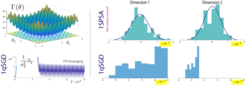
Figure 8: Rastrigin objective (top left), scaled empirical covariance (bottom left), histograms of estimation error for $1$SPSA with PR averaging (top middle and top right), histograms of estimation error for $1$qSGD with PR averaging (bottom middle and bottom right).

Results

Fig. 8 shows plots for the scaled empirical covariance for $1$qSGD as well as histograms for the estimation error $\Uptheta^{\text{\tiny\sf PR}}_{T}-\theta^{*}$ for both algorithms. We see in Fig. 8 that the convergence rates of $O(T^{-2\rho})$ are achieved by both filtering techniques.

The variance of the estimation error for the deterministic algorithm is much smaller than for its stochastic counterpart: Fig. 8 shows that the reduction is roughly two orders of magnitude.

Outliers were identified with Matlab’s isoutlier function and removed from the histograms in Fig. 8. Around $40\%$ of the estimates were considered outliers for the stochastic algorithm, while none was observed for its deterministic counterpart.

Recall that bias is inherent in both 1qSGD and 1SPSA when using a non-vanishing probing gain. It would appear from Fig. 8 that this bias is larger for 1qSGD [consider the histogram for estimates of $\theta_{1}^{*}=0$, which shows that final estimates typically exceed this value]. In fact, there is no theory to predict if 1qSGD is better or worse than 1SPSA in terms of bias. The bias is imperceptible in the stochastic case due to the higher variance combined with the removal of outliers.

4.2 Vanishing vs Fixed Gain Algorithms - Rastrigin’s Objective

Experiments were performed to test the performance of the Lipschitz version of $1$qSGD for both constant and vanishing gain algorithms. Two take-aways from the numerical results surveyed below:

• The value of a second order filter can be substantial when using a fixed gain algorithm. Recall that this conclusion was not at all clear for either of the linear examples (54a, 54b), even though in the first case the example satisfies the assumptions of Thm. 2.7.

• However, in this example the flexibility of a vanishing gain algorithm is evident: with high gain during the start of the run (when $a_{t}\approx\alpha$) there is a great deal of exploration, especially when $\Uptheta_{t}$ is far from the optimizer due to the use of $\upepsilon(\theta)$. The vanishing gain combined with the use of distinct frequencies then justifies the use of PR-averaging, which results in extremely low AAD in this example.

Simulation Setup

For this objective, $M=5$ individual experiments were carried out in a similar fashion to the experiments summarized in Section 4.1. The Lipschitz variant of $1$qSGD was implemented using each of the initial conditions so projection of the sample paths $\{\Uptheta^{m}_{t}\}$ was not necessary. Each experiment used $\upepsilon(\theta)=\varepsilon\sqrt{1+\|\theta\|^{2}}$ with $\varepsilon=0.6$ and the same probing signal ${\scalebox{1.1}{$\upxi$}}^{m}_{t}$ as in (99). The following three choices of gain were tested for each initial condition:

$$\text{(a) }a_{t}=0.1(t+1)^{-0.65}\quad\text{(b) }a_{t}=\alpha_{b}=3\times 10^{-3}\quad\text{(c) }a_{t}=\alpha_{s}=7\times 10^{-4}$$

For the vanishing gain case (a) the process $\{\Uptheta^{m}_{t}\}$ was accelerated through PR averaging with $\kappa=5$, while for the fixed-gain case two filters of the form (55) where used with $\zeta=0.8$ and $\gamma=\eta\alpha$ for various values of $\eta\geq 1$. These experiments were repeated for $\Uptheta^{m}_{0}$ uniformly sampled from $10^{10}[-B,B]^{2}$ with $B=5.12$.

Results

The top row of Fig. 9 shows the evolution of $\{\Uptheta^{m}_{t}\}$ for each $m$ with $\eta=5$. The second row shows the evolution of $\{\Upgamma(\Uptheta^{\text{\tiny\sf PR}}_{T}),\Upgamma({\Uptheta}^{1\text{\tiny\sf F}}_{T}),\Upgamma({\Uptheta}^{2\text{\tiny\sf F}}_{T}),\Upgamma(\Uptheta_{T})\}$ for the single path yielding the best performance for each gain choice across all 5 initial conditions.

We see in Fig. 9 a clear advantage of vanishing gain algorithms: the algorithm explores much more in the beginning of the run, eventually deviating from $\theta^{\text{\tiny\sf opt}}$ by the bias inherent to the $1$qSGD algorithm.

For the runs that used $\alpha_{b}$ (case (b)), we have a good amount of exploration, but the steady state behavior is poor. Case (c) using the smaller value of $\alpha$ yielded better results.

Fig. 9 shows the benefit of variance reduction from second order filter as opposed to a first order filter, based on runs that used $\alpha_{s}$. As opposed to the results in Fig. 5, this example shows that we can’t always obtain the best AAD with a first order filter. For these experiments, the filtered final estimation of $\theta^{*}$ yields comparable objective values to what is seen in the vanishing gain experiment. However, we do not always observe desirable exploration as in the vanishing gain case: we see several sample paths hovering around local minima of the objective rather than $\theta^{\text{\tiny\sf opt}}$.

Results for the trajectories with initial conditions of order $10^{10}$ were presented in Fig. 2.

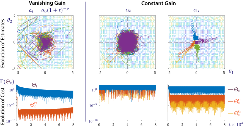
Figure 9: Comparison of the performance between vanishing and constant gain $1$qSGD for the Rastrigin Objective.

4.3 The Walking Camel

The next numerical results are based on a tracking problem using the $1$qSGD algorithm. Although the results in this subsection will show that the algorithm successfully tracks the signal $\{\theta^{\text{\tiny\sf opt}}_{t}\}$, we are not advocating the use of $1$qSGD for tracking applications. The algorithm was employed to illustrate general algorithm design principles; better performance is likely in algorithms with a carefully designed low pass filter such as (80) with $\sigma>0$. Several experiments were conducted to address the following questions:

• How does the frequency content of the probing signal affect performance?

• How does the rate of change of the signal $\{\theta^{\text{\tiny\sf opt}}_{t}\}$ impact tracking performance?

• How does filtering reduce estimation error and variance in tracking?

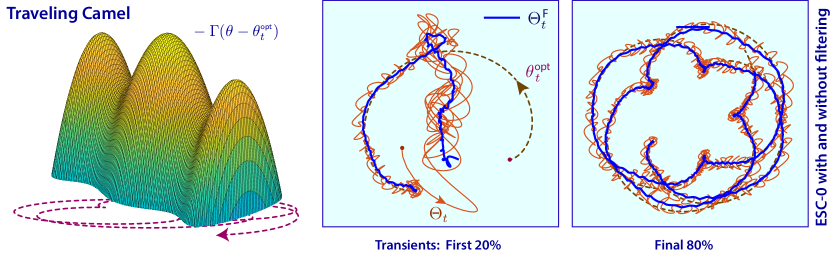
Figure 10: Tracking for the travelling camel with ESC-0

Simulation Setup

The Three-Hump Camel objective is the sixth-order polynomial function on $\mathbb{R}^{2}$:

$$\Upgamma(\theta)=2\theta_{1}^{2}+\theta_{1}\theta_{2}+\theta_{2}^{2}+\tfrac{1}{6}\theta_{1}^{6}-1.05\theta_{1}^{4}$$ (101)

A plot of the negative of this objective is shown on the left hand side of Fig. 10. Observe that the infimum of $\Upgamma$ over $\mathbb{R}^{2}$ is not finite. The domain of this function is usually taken to be the bounded region $[-5,5]^{2}$ [53].

We considered a time varying version, of the form

$$\Upgamma_{t}=\Upgamma(\theta-\theta^{\text{\tiny\sf opt}}_{t})$$

with the following choices of $\{\theta^{\text{\tiny\sf opt}}_{t}\}$:

$$\text{(a) }\theta^{\text{\tiny\sf opt}}_{t}=\begin{bmatrix}m\cos(\omega^{\circ}t)-h\cos(m\omega^{\circ}t/b^{\circ})\\ m\sin(\omega^{\circ}t)-h\sin(m\omega^{\circ}t/b^{\circ})\end{bmatrix}\quad\text{where }\omega^{\circ}=2\times 10^{-3}~{}\text{rad/sec},b^{\circ}=3/5,m=8/5,h=0.6$$ (102)

$$\text{(b) }\theta^{\text{\tiny\sf opt}}_{t}=\begin{bmatrix}1\\ 1\end{bmatrix}g_{t},\quad\text{where }g_{t}=\begin{cases}\Delta(t/T_{0}),&t\leq T/2\\ \Pi(t/T_{0}),&t>T/2\end{cases}\quad\text{and }T_{0}=\frac{c}{b}~{}\text{sec with }b\in\{1,3,5\},c=5\times 10^{-3}$$

The choice (a) is an example of an epitrochoid path. In (b) the notation $\Delta,\Pi$ is used to denote the unit triangle and square waves, respectively. The objective $\Upgamma_{t}$ was normalized so that $\theta^{\text{\tiny\sf opt}}={\mathchoice{{\mathchoice{\mbox{\large\sf 0}}{\mbox{\large\sf 0}}{\mbox{\tiny\sf 0}}{\mbox{\tiny\sf 0}}}}{\mbox{\sf 0}}{\mbox{\tiny\sf 0}}{\mbox{\tiny\sf 0}}}$.

Experiments were conducted for a single initial condition $\Uptheta_{0}$, chosen to be a second (non-optimal) local minima of the objective, and the following probing signals:

$${\scalebox{1.1}{$\upxi$}}^{a}_{t}=2\begin{bmatrix}\sin(t/9)\\ \sin(t/e^{3})\end{bmatrix},\quad{\scalebox{1.1}{$\upxi$}}^{b}_{t}=2\begin{bmatrix}\sin(t/4)\\ \sin(t/e^{2})\end{bmatrix},\quad{\scalebox{1.1}{$\upxi$}}^{c}_{t}=2\begin{bmatrix}\sin(\sqrt{20}t/10)\\ \sin(\pi t/10)\end{bmatrix}$$ (103)

The assumptions of Prop. 3.1 are violated in this example, since the gradient of this objective is not Lipschitz continuous. For this reason, the state-dependent gain $\upepsilon$ was abandoned in favor of a constant gain in these experiments. Choices for the parameters $\upepsilon(\theta)\equiv\varepsilon$ and $\alpha$ were problem specific: (a) $\varepsilon=0.2$ and $\alpha=6\times 10^{-3}$, (b) $\varepsilon=0.5$ and $\alpha=5\times 10^{-3}$.

The process $\{\Uptheta_{t}\}$ was projected onto the set $[-5,5]^{2}$. The filters in (55) were used for variance reduction, with $\zeta=0.8$ and $\gamma=\eta\alpha$ for several $\eta\geq 1$.

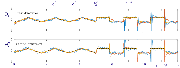
Figure 11: Tracking of $\{\theta^{\text{\tiny\sf opt}}_{t}\}$ for several choices of probing signal.

Results

Case (a)  Phase plots of the trajectories $\{\Uptheta_{t}\},\{{\Uptheta}^{1\text{\tiny\sf F}}_{t}\}$ are shown in Fig. 10. These plots display results with the probing signal ${\scalebox{1.1}{$\upxi$}}^{b}_{t}$ and $\eta=5$. It is possible to see in Fig. 10 that the output of $1$qSGD tracks $\{\theta^{\text{\tiny\sf opt}}_{t}\}$ after a transient period. Since the gain is non-vanishing, $\bm{\Uptheta}$ oscillates around the trajectory $\{\theta^{\text{\tiny\sf opt}}_{t}\}$. As expected by Thm. 2.7, the filtered process has much less variability.

Case (b)  Fig. 11 shows the evolution of $\{\Uptheta_{t}\}$ using each probing signal in (103). Here, the signal $\{\theta^{\text{\tiny\sf opt}}_{t}\}$ has period $T_{0}$ with $b=3$ (102). The plots in Fig. 11 illustrate how the frequency content of the probing signal impacts tracking performance: higher frequencies yield less variability over most of the run.

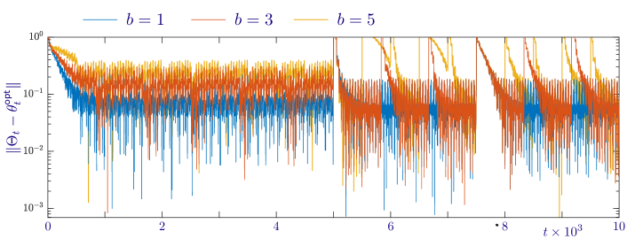
Figure 12: Estimation error for different $b$ (102).

The evolution of the estimation error $\{\|\Uptheta_{t}-\theta^{\text{\tiny\sf opt}}_{t}\|\}$ is shown in Fig. 12 for each value of $b$ listed in (102). Only ${\scalebox{1.1}{$\upxi$}}^{c}_{t}$ in (103) was used as the probing signal for these experiments. We see in Fig. 12 that tracking performance deteriorates as the rate of change of $\{\theta^{\text{\tiny\sf opt}}_{t}\}$ increases. When $t>T/2$, the signal $\{\theta^{\text{\tiny\sf opt}}_{t}\}$ is nearly static for each period and hence we expect the rate of change of $\{\theta^{\text{\tiny\sf opt}}_{t}\}$ to have little effect on the AAD. This is confirmed by the results in shown in Fig. 12: the steady state estimation errors are roughly the same for all values of $b$.

Fig. 13 shows the evolution $\{\Upgamma(\Uptheta_{t}),\Upgamma({\Uptheta}^{1\text{\tiny\sf F}}_{t}),\Upgamma({\Uptheta}^{2\text{\tiny\sf F}}_{t})\}$ as functions of time for $\eta\in\{5,15\}$. Again, the selected probing signal was ${\scalebox{1.1}{$\upxi$}}^{c}_{t}$ and the signal $\{\theta^{\text{\tiny\sf opt}}_{t}\}$ had period $T_{0}$ with $b=3$ for both choices of $\eta$. We see in Fig. 13 that the filtered estimates $\{{\Uptheta}^{1\text{\tiny\sf F}}_{t}\}$ yield lower objective values than $\{{\Uptheta}^{2\text{\tiny\sf F}}_{t}\}$ for $t\leq T/2$. When $t>T/2$, the estimates $\{{\Uptheta}^{1\text{\tiny\sf F}}_{t}\}$ only yield lower objective values than $\{{\Uptheta}^{2\text{\tiny\sf F}}_{t}\}$ for very small portions of the run. That is, a second order filter is preferable when the rate of change of $\{\theta^{\text{\tiny\sf opt}}_{t}\}$ is small.

Recall that the parameter $\eta$ scales the bandwidth of the filter. We see in Fig. 13 an improvement in tracking for both filters when $\eta$ is increased as a consequence of the increased bandwidth.

Figure 13: Evolution of $\Upgamma$ for different filtering techniques.

5 Conclusions

This paper introduces a new exact representation of the QSA ODE, opening several doors for analysis. Major outcomes of the perturbative mean flow representation include the clear path to obtaining transient bounds based on those of the mean flow, and guidelines on how to design filters to obtain bias and AAD of order $O(\alpha^{2})$. There is much more to be unveiled:

$\triangle$  The use of filtering for acceleration of algorithms is not at all new. It will be exciting to investigate the implications of the acceleration techniques pioneered by Polyak and Nesterov for nonlinear optimization, particularly in their modern form (see [28, § 2.2] and the references therein).

The integration of these two disciplines may provide insight on how to design the high pass filters shown in Fig. 3, or suggest entirely new architectures.

$\triangle$  The introduction of normalization in the observations in the general form (85) was crucial to obtain global stability of ESC ODEs. There are many improvements to consider. First, on considering the Taylor series approximation (86), performance is most likely improved via a second normalization:

$$\mathcal{Y}^{\text{\footnotesize\sf n}}_{t}=\frac{1}{\upepsilon_{t}}\Bigl{[}\Upgamma(\Uptheta_{t}+\upepsilon_{t}{\scalebox{1.1}{$\upxi$}}_{t})-\Upgamma^{\star}_{t}\Bigr{]}\,,$$

in which $\{\Upgamma^{\star}_{t}\}$ are estimates of the minimum of the objective. These might be obtained by passing $\{{\cal Y}_{r}\mathbin{:=}\Upgamma(\Uptheta_{r}+\upepsilon_{r}{\scalebox{1.1}{$\upxi$}}_{r})\}$ through a low pass filter.

$\triangle$  Far better performance might be obtained through an observation process inspired by 2SPSA. Consider first a potential improvement of 2SPSA: A state dependent exploration gain is introduced, so that (22b) becomes

$$\theta_{n+1}=\theta_{n}-\alpha_{n+1}\frac{1}{2\varepsilon}{\scalebox{1.1}{$\upxi$}}_{n+1}\bigl{[}\Upgamma(\theta_{n}+\upepsilon_{n}{\scalebox{1.1}{$\upxi$}}_{n+1})-\Upgamma(\theta_{n}-\upepsilon_{n}{\scalebox{1.1}{$\upxi$}}_{n+1})\bigr{]}\,$$

with $\upepsilon_{n}=\upepsilon(\theta_{n})$. The division by $2\varepsilon$ (independent of state) remains, since 2SPSA in its original form satisfies the required Lipschitz conditions for SA provided $\nabla\Upgamma$ is Lipschitz continuous.

There are surely many ways to obtain an online version based on QSA. One approach is through sampling: denote $T_{n}=nT$ for a given sampling interval $T>0$, and take $\mathcal{Y}^{\text{\footnotesize\sf n}}_{t}$ constant on each interval $[T_{n},T_{n+1})$, designed to mimic 2SPSA. One option is the simple average,

$$\mathcal{Y}^{\text{\footnotesize\sf n}}_{T_{n+1}}\mathbin{:=}\frac{2}{T}\frac{1}{2\varepsilon} \int_{T_{n}}^{T_{n}+T/2}{\scalebox{1.1}{$\upxi$}}_{t}\bigl{[}\Upgamma(\theta_{n}+\upepsilon_{t}{\scalebox{1.1}{$\upxi$}}_{t})-\Upgamma(\theta_{n}-\upepsilon_{t}{\scalebox{1.1}{$\upxi$}}_{t})]\,dt$$

with $\theta_{n}=\Uptheta_{T_{n}}$. This can be computed in real-time, based on two sets of observations:

$$\Upgamma(\theta_{n}+\upepsilon_{t}{\scalebox{1.1}{$\upxi$}}_{t}) T_{n}\leq t\leq T_{n}+T/2$$

$$\Upgamma(\theta_{n}-\upepsilon_{n}{\scalebox{1.1}{$\upxi$}}_{t-T/2}) T_{n}+T/2\leq t\leq T_{n+1}$$

$\triangle$  The implications to reinforcement learning deserve much greater attention. The applications of QSA and ESC in [33, 21, 34] are only a beginning.

$\triangle$  It may be straightforward to extend the P-mean flow representation (12) to tracking problems. This may start with the general topic of time inhomogeneous QSA, of the form

$${\mathchoice{\genfrac{}{}{}{1}{d}{dt}}{\genfrac{}{}{}{1}{d}{dt}}{\genfrac{}{}{}{3}{d}{dt}}{\genfrac{}{}{}{3}{d}{dt}}}\Uptheta_{t}=\alpha f(\Uptheta_{t},{\scalebox{1.1}{$\upxi$}}_{t};t)\,.$$

Analysis would require consideration of solutions to Poisson’s equation, such as ${\hat{f}}(\theta,\,\cdot\,;t)$ for each $\theta\in\mathbb{R}^{d}$ and $t\in\mathbb{R}$. The representation will be more complex than (12), but will likely lead to sharper bounds than are presently available.

6 Literature and Resources

Background on stability via Lyapunov criteria is standard [7, 23]. The ODE@$\infty$ approach was introduced in [8], and refined in a series of papers since [4, 45, 6].

Quasi-stochastic approximation:  The first appearance of the QSA ODE is the almost periodic linear system discussed in Section 2.5.1—see [30, 52] for the century-old history.

The first work on QSA as an alternative to SA appears in [24, 25] with applications to finance, and [5] contains initial results on convergence rates that are better than that obtained for their stochastic counterparts, but nothing like the bounds obtained here. The setting for this prior work is in discrete time.

The QSA ODE appeared in applications to reinforcement learning in [33], which motivated the convergence rate bounds in [50] for multi-dimensional linear models, of which (2.3) are special cases (except that analysis is restricted to vanishing gain algorithms).

The work of [50] was extended to nonlinear QSA in [10, 11], and initial results on PR averaging and the challenges with multiplicative noise is one topic of [34, § 4.9]. Until recently it was believed that the best convergence rate possible is $O(1/T)$ for the vanishing gain algorithms considered. Recently, this was shown to be fallacy: convergence rates arbitrarily close to $O(T^{-2})$ are obtained in [26] via PR-averaging, but again this requires that a version of $\Upupsilon$ be zero.

Extremum seeking control:  ESC is perhaps among the oldest gradient-free optimization methods. It was born in the 1920s when a extremum seeking control solution was developed to maintain maximum transfer of power between a transmission line and a tram car [27, 54, 29]. Successful stories of the application of ESC to various problems have been shared over the 20th century – e.g. [46, 47, 15, 32, 39], but theory was always behind practice: the first Lyapunov stability analysis for ESC algorithms appeared in the 70s for a very special case [31].

General local stability and bounds on estimation error for ESC with scalar-valued probing signals were established 30 years later in [22] and later extended for multi-dimensional probing in [2], but the authors do not specify a domain of attraction for stability. Stronger stability results was than established in [55], where the authors show that for an arbitrarily large set of initial conditions, it is possible to find control parameters so that the extermum seeking method results in a solution arbitrarily close the extrema to be found. This is known as semi-global pratical stability in the ESC literature. These analytical contributions sparked further research [14, 20, 17, 41].

It is pointed out in [36] that there is a potential “curse of dimensionality” when using sinusoidal probing signals, which echos the well known curse in Quasi Monte Carlo [3].

Convergence rates for stochastic approximation:  Consider first the case of vanishing step-size: with step-size $\alpha_{n}=(1+n)^{-\rho}$, ${\mathchoice{\genfrac{}{}{}{1}{1}{2}}{\genfrac{}{}{}{1}{1}{2}}{\genfrac{}{}{}{3}{1}{2}}{\genfrac{}{}{}{3}{1}{2}}}<\rho<1$, we obtain the following limits for the scaled asymptotic mean-square error (AMSE):

$$\lim_{n\to\infty}\frac{1}{\alpha_{n}}{\sf E}[\|\theta_{n}-\theta^{*}\|^{2}] =\hbox{\rm trace\,}(\Sigma_{\theta}(\rho))$$ (104)

$$\lim_{n\to\infty}n{\sf E}[\|\theta^{\text{\tiny\sf PR}}_{n}-\theta^{*}\|^{2}] =\hbox{\rm trace\,}(\Sigma_{\theta}^{*})$$ (105)

where $\{\theta^{\text{\tiny\sf PR}}_{n}\}$ are obtained from $\{\theta_{n}\}$ via Polyak-Ruppert averaging (26). The covariance matrix in the second limit has the explicit form $\Sigma_{\theta}=G\Sigma_{\Delta}G^{\intercal}$ with $G={A^{*}}^{-1}$ and $\Sigma_{\theta}$ the covariance of $f(\theta^{*},{\scalebox{1.1}{$\upxi$}}_{n+1})$ (see (2)). The covariance matrix $\Sigma_{\theta}^{*}$ is minimal in a strong sense [40, 6, 7, 23].

There is an equally long history of analysis for algorithms with constant gains. For simplicity assume an SA algorithm with $\bm{\upxi}$ i.i.d., so that the stochastic process $\theta$ is a Markov chain. Stability of the ODE@$\infty$ implies a strong form of geometric ergodicity under mild assumptions on the algorithm [8], which leads to bounds on the variance

$${\sf E}[\|\theta_{n}-\theta^{*}\|^{2}]={\sf E}[\|\theta_{\infty}-\theta^{*}\|^{2}]+O(\varrho^{n})$$ (106)

where the steady-state mean ${\sf E}[\|\theta_{\infty}-\theta^{*}\|^{2}]$ is of order $O(\alpha)$ with step-size $\alpha>0$, and $\varrho<1$ since $\theta$ is geometrically ergodic. Averaging can reduce variance significantly [37, 16].

Zeroth order optimization:  We let $\theta^{*}$ denote the limit of the algorithm (assuming it exists), and $\theta^{\text{\tiny\sf opt}}$ the global minimizer of $\Upgamma$.

We begin with background on methods based on stochastic approximation, which was termed gradient free optimization (GFO) in the introduction.

1. GFO   Much of the theory is based on vanishing gain algorithms, and the probing gain is also taken to be vanishing in order to establish that the algorithm is asymptotically unbiased.

Polyak was also a major contributor to the theory of convergence rates for GFO algorithms that are asymptotically unbiased, with [44] a highly cited starting point. If the objective function is $p$-fold differentiable at $\theta^{*}$ then the best possible rate for the AMSE is $O(n^{-\beta})$ with $\beta=\frac{p-1}{2p}$. This work was motivated in part by the upper bounds and algorithms of Fabian [18]. See [13, 12, 40] for more recent history, and algorithms based on averaging that achieve this bound; typically using averaging combined with vanishing step-sizes.

2. ESC  Theory has focused on constant-gain algorithms because many authors are interesting in tracking rather than solving exactly a static optimization problem.

It is shown in [22], that it is possible to implement ESC to find a control law that drives a system near to an equilibrium state $x^{\text{\tiny\sf opt}}$, minimizing the steady-state value of its output at $-y^{\text{\tiny\sf opt}}$. It is assumed that $x^{\text{\tiny\sf opt}}=\Upgamma(\theta^{\text{\tiny\sf opt}})$ where $\Upgamma:\mathbb{R}\to\mathbb{R}^{d}$ is a smooth function. For a scalar-valued perturbation signal of the form ${\scalebox{1.1}{$\upxi$}}_{t}=\alpha\sin(\omega t)$, the estimation error $\|y^{*}-y^{\text{\tiny\sf opt}}\|$ is of order $O(\alpha^{2})$, assuming stability of the algorithm. These results are later extended to the case where $\theta,{\scalebox{1.1}{$\upxi$}}\in\mathbb{R}^{d}$ in [2] satisfying: ${\scalebox{1.1}{$\upxi$}}^{j}_{t}=\alpha\sin(\omega_{j}t)$, for $\{1\leq j\leq d\}$. In this multivariate setting, the function $\Upgamma:\mathbb{R}^{d}\to\mathbb{R}^{d}$ was assumed to be quadratic and time-varying. It is shown that the estimation error for tracking is not only a function of $\alpha$ but also the frequencies of $\upxi$ , since $\|y^{*}-y^{\text{\tiny\sf opt}}\|$ was of order $O(1/\omega^{2}_{1}+d^{2}\alpha^{2})$ where $\omega_{1}$ is the smallest frequency among $\{\omega_{j}\}$.

Appendix A Appendix

A.1 ODE QSA Solidarity

The first step in the proof of Prop. 2.11 is to re-interpret the LLN (35):

Lemma A.1.

If (A1) holds then the following uniform Law of Large Numbers holds: there is a function $\varepsilon_{f}\colon\mathbb{R}\to\mathbb{R}_{+}$ such that for any $\theta\in\mathbb{R}^{d}$ and $\Phi_{0}\in\Upomega$,

$$\left|\frac{1}{T}\int_{0}^{T}\bigl{[}f(\theta,{\scalebox{1.1}{$\upxi$}}^{\alpha}_{t})-{\widebar{f}}(\theta)\bigr{]}\,dt\right|\leq\bigl{(}1+\|\theta\|\bigr{)}\varepsilon_{f}(T/\alpha)$$ (108)

with $\varepsilon_{f}(r)\to 0$ as $r\to\infty$.

Armed with this lemma, we now compare solutions to (62) with solutions to the mean flow (4). If both are initialized at the same value $\upvartheta_{0}=\Uptheta_{0}=\theta_{0}$, we obtain for any $T>0$,

$$\Uptheta^{\alpha}_{T}=\theta_{0}+\int_{0}^{T}f(\Uptheta_{r}^{\alpha},{\scalebox{1.1}{$\upxi$}}^{\alpha}_{r})\,dr\,,\qquad\upvartheta_{T}=\theta_{0}+\int_{0}^{T}{\widebar{f}}(\upvartheta_{r})\,dr$$

The challenge is that the bound (108) holds with $\theta$ fixed, so that it is not immediately applicable to comparison of the two ODEs.

To proceed we divide the positive real line into adjacent intervals $[\tau_{n},\tau_{n+1})$, and let $\{\upvartheta^{n}_{t}:t\geq\tau_{n}\}$ denote the solution to (4) with $\upvartheta^{n}_{\tau_{n}}=\Uptheta^{\alpha}_{\tau_{n}}$. We take $\tau_{n}=\Delta n$ for each $n$, with $\Delta\in(0,1]$ to be chosen as a function of $\alpha\leq 1$. The following corollary to Lemma A.1 will provide constraints on this choice.

Lemma A.2.

The following uniform bounds hold under (A1): for a fixed constant $B_{f}$, and each $n\geq 0$,

$$\|\upvartheta^{n+1}_{\tau_{n+1}}-\upvartheta^{n}_{\tau_{n+1}}\|=\|\Uptheta^{\alpha}_{\tau_{n+1}}-\upvartheta^{n}_{\tau_{n+1}}\|\leq\Delta B_{f}^{n}(\Delta,\alpha)\mathbin{:=}B_{f}\Delta^{2}+\Delta[1+\|\upvartheta^{n}_{\tau_{n}}\|]\varepsilon_{f}(\Delta/\alpha)$$

The proof of the lemma relies on Lemma A.1 and an application of the Bellman-Grönwall inequality:

Lemma A.3.

Let $\bm{\upvartheta}^{i}$, $i=1,2$, denote two solutions to (4), with different initial conditions. Then, subject to (A1),

$$\|\upvartheta^{1}_{t}-\upvartheta^{2}_{t}\|\leq\|\upvartheta^{1}_{0}-\upvartheta^{2}_{0}\|e^{L_{f}t}\,,\qquad t\geq 0.$$

Proof of Lemma A.2.

The equality $\|\upvartheta^{n+1}_{\tau_{n+1}}-\upvartheta^{n}_{\tau_{n+1}}\|=\|\Uptheta^{\alpha}_{\tau_{n+1}}-\upvartheta^{n}_{\tau_{n+1}}\|$ follows from the definitions. To bound the latter, we write

$$\Uptheta^{\alpha}_{\tau_{n+1}}-\upvartheta^{n}_{\tau_{n+1}} =\int_{\tau_{n}}^{\tau_{n+1}}\bigl{[}f(\Uptheta^{\alpha}_{r},{\scalebox{1.1}{$\upxi$}}^{\alpha}_{r})-{\widebar{f}}(\upvartheta^{n}_{r})\bigr{]}\,dr$$ Bounds:

$$=\int_{\tau_{n}}^{\tau_{n+1}}\bigl{[}f(\Uptheta^{\alpha}_{\tau_{n}},{\scalebox{1.1}{$\upxi$}}^{\alpha}_{r})-{\widebar{f}}(\upvartheta^{n}_{\tau_{n}})\bigr{]}\,dr O\bigl{(}\bigl{(}1+\|\upvartheta^{n}_{\tau_{n}}\|\bigr{)}\varepsilon_{f}(\Delta/\alpha)\bigr{)}$$

$$\quad+\int_{\tau_{n}}^{\tau_{n+1}}\bigl{[}f(\Uptheta^{\alpha}_{r},{\scalebox{1.1}{$\upxi$}}^{\alpha}_{r})-f(\Uptheta^{\alpha}_{\tau_{n}},{\scalebox{1.1}{$\upxi$}}^{\alpha}_{r})\bigr{]}\,dr\qquad O\bigl{(}\Delta^{2}\bigr{)}$$

$$\quad+\int_{\tau_{n}}^{\tau_{n+1}}\bigl{[}{\widebar{f}}(\upvartheta^{n}_{\tau_{n}})-{\widebar{f}}(\upvartheta^{n}_{r})\bigr{]}\,dr O\bigl{(}\Delta^{2}\bigr{)}$$

That is, the error is the sum of three terms, in which the first is bounded via Lemma A.1, and the second two are bounded by $O(\Delta^{2})$ for $\Delta\leq 1$ under the Lipschitz assumptions on $f$ and ${\widebar{f}}$.     $\sqcap$$\sqcup$

The next step is to obtain uniform bounds on the error ${\cal E}_{n}=\|\upvartheta^{n}_{\tau_{n}}-\upvartheta_{\tau_{n}}\|$ for each $n$, with $\upvartheta_{\tau_{n}}$ the solution at time $\tau_{n}$ with initial condition $\upvartheta_{0}=\Uptheta_{0}=\theta_{0}$, so in particular ${\cal E}_{0}=0$.

Lemma A.4.

The following uniform bounds hold under (A1), provided $\varepsilon_{f}(\Delta/\alpha)\leq 1$: for a fixed constant $B_{f}^{1}$, and each $n\geq 0$,

$$\|\upvartheta^{n}_{\tau_{n}}-\upvartheta_{\tau_{n}}\|\leq B_{f}^{1}\exp(2L_{f}\tau_{n})\bigl{[}1+\|\theta_{0}\|\bigr{]}\cdot\bigl{[}\Delta+\varepsilon_{f}(\Delta/\alpha)\bigr{]}$$

Proof.

The proof begins with the triangle inequality to obtain a recursive bound:

$${\cal E}_{n+1}\mathbin{:=}\|\upvartheta^{n+1}_{\tau_{n+1}}-\upvartheta_{\tau_{n+1}}\| \leq\|\upvartheta^{n}_{\tau_{n+1}}-\upvartheta_{\tau_{n+1}}\|+\|\upvartheta^{n+1}_{\tau_{n+1}}-\upvartheta^{n}_{\tau_{n+1}}\|$$

$$\leq\|\upvartheta^{n}_{\tau_{n+1}}-\upvartheta_{\tau_{n+1}}\|+\Delta B_{f}^{n}(\Delta,\alpha)$$

The recursion is obtained on combining this bound with Lemma A.3:

$${\cal E}_{n+1}\leq e^{L_{f}\Delta}\|\upvartheta^{n}_{\tau_{n}}-\upvartheta_{\tau_{n}}\|+\Delta B_{f}^{n}(\Delta,\alpha)=e^{L_{f}\Delta}{\cal E}_{n}+\Delta B_{f}^{n}(\Delta,\alpha)$$

where $B_{f}^{n}$ appears in Lemma A.2. Applying the triangle inequality,

$$B_{f}^{n}(\Delta,\alpha)=B_{f}\Delta+[1+\|\upvartheta^{n}_{\tau_{n}}\|]\varepsilon_{f}(\Delta/\alpha)\leq\bigl{(}B_{f}\Delta+\varepsilon_{f}(\Delta/\alpha)\bigr{)}+\bigl{(}\|\upvartheta_{\tau_{n}}\|+{\cal E}_{n}\bigr{)}\varepsilon_{f}(\Delta/\alpha)$$

An application of Lemma A.3 once more gives $\|\upvartheta_{\tau_{n}}\|\leq e^{L_{f}\tau_{n}}\|\theta_{0}\|$.

Combining these bounds gives

$${\cal E}_{n+1} \leq\beta_{\Delta}{\cal E}_{n}+\Delta\bigl{[}{\cal U}^{0}+{\cal U}^{1}e^{L_{f}\tau_{n}}\bigr{]}$$

  with $$\beta_{\Delta}\mathbin{:=}e^{L_{f}\Delta}+\varepsilon_{f}(\Delta/\alpha)$$

$${\cal U}^{0}\mathbin{:=}\bigl{(}B_{f}\Delta+\varepsilon_{f}(\Delta/\alpha)\bigr{)}\,,\quad{\cal U}^{1}\mathbin{:=}\varepsilon_{f}(\Delta/\alpha)\|\theta_{0}\|$$

The final bound is obtained by iteration, and recalling ${\cal E}_{0}=0$.

It is simplest to obtain a comparison with the ordinary differential equation,

$${\mathchoice{\genfrac{}{}{}{1}{d}{dt}}{\genfrac{}{}{}{1}{d}{dt}}{\genfrac{}{}{}{3}{d}{dt}}{\genfrac{}{}{}{3}{d}{dt}}}X_{t}=\gamma_{\Delta}X_{t}+{\cal U}^{0}+{\cal U}^{1}\exp(L_{f}t)\,,\quad X_{0}={\cal E}_{0}=0$$

with $\gamma_{\Delta}=(\beta_{\Delta}-1)/\Delta$.     $\sqcap$$\sqcup$

Proof of Prop. 2.11.

Combining Lemma A.2 and Lemma A.4 we obtain the bound Prop. 2.11 for the sampling times $\tau_{n}$, provided we choose $\Delta=\Delta(\alpha)$ so that

$$\varepsilon_{0}(\alpha)\mathbin{:=}\Delta(\alpha)+\varepsilon_{f}(\Delta(\alpha)/\alpha)\to 0\,,\quad\textit{as $\alpha\downarrow 0$}$$

For this we choose $\Delta=\alpha^{\rho}$ with $\rho\in(0,1)$.

Lipschitz continuity of $f$ and ${\widebar{f}}$ implies that the bound (63) is preserved for all time, with an increase in $B_{0}$ by a value of only $O(\Delta)$.     $\sqcap$$\sqcup$

A.2 Baker’s Theorem and Poisson’s Equation

Here we explain how to obtain well behaved solutions to Poisson’s equation for a function $h\colon\mathbb{R}^{d}\to\mathbb{R}$ that is is analytic. We denote the mixed partials by

$$h^{(\beta)}(z)=\frac{\partial^{\beta_{1}}}{\partial z_{1}^{\beta_{1}}}\cdots\frac{\partial^{\beta_{d}}}{\partial z_{d}^{\beta_{d}}}h\,(z)\,,\quad\beta\in\mathbb{Z}_{+}^{d}\,.$$

For $\beta\in\mathbb{Z}_{+}^{d}$ and a vector $v\in\mathbb{R}^{d}$ we denote $v^{\beta}=v_{1}^{\beta_{1}}\cdots v_{d}^{\beta_{d}}$, and $|\beta|$ the $\ell_{1}$ norm: $|\beta|=\sum|\beta_{i}|$.

A candidate representation for ${\hat{h}}$ can be found on obtaining the solution to Poisson’s equation for each of the primitive functions appearing in a Taylor series expansion. Justification is then a challenge without assumptions on the frequencies.

For any $\beta\in\mathbb{Z}^{K}$ denote $\omega_{\beta}=\sum\beta_{i}\omega_{i}$ and $\phi_{\beta}=\sum\beta_{i}\phi_{i}$. We will see that the terms in the Taylor series expansion for ${\hat{h}}$ resemble those for $h$, but with terms divided by $\omega_{\beta}$ (subject to the constraint that this is non-zero). Consequently, a lower bound on $\omega_{\beta}$ as a function of $|\beta|$ is required—such bounds are available under Assumption (A0).

The proof of the following in the almost periodic setting is based on a version of Baker’s Thereom [9, Thm. 1.8]: there is a constant $C>0$ such that for any $\beta$, provided $\omega_{\beta}\neq 0$,

$$|\omega_{\beta}|\geq k_{\beta}^{-C}\,,\quad k_{\beta}=\max\{3,\beta_{1},\dots,\beta_{d}\}$$

The periodic case is much simpler since in this case $|\omega_{\beta}|\geq\omega_{1}$ whenever $\omega_{\beta}$ is non-zero.

Theorem A.5.

Suppose that $h\colon\mathbb{R}^{K}\to\mathbb{R}$ is analytic. Then there are coefficients $\{c_{\beta}:\beta\in\mathbb{Z}^{K}\}$ such that the following representations hold for $h$ and its mean ${\overline{h}}$:

$$h({\scalebox{1.1}{$\upxi$}}_{t}) =\sum_{\beta\in\mathbb{Z}^{K}}c_{\beta}\cos(2\pi[\omega_{\beta}t+\phi_{\beta}])\,,\qquad{\overline{h}}=\sum_{\beta:\omega_{\beta}=0}c_{\beta}\cos(2\pi\phi_{\beta})$$ (109a)

If in addition the frequencies $$\{\omega_{i}\} {\hat{h}} \{\mathbb{C}\setminus\{0\}\}^{K} \Upomega$$ satisfy either of the conditions (33b), then there is a solution to Poisson’s equation that has zero mean, and is analytic on the domain . When restricted to it takes the form,

$${\hat{h}}(\Phi_{t})=-\frac{1}{2\pi}\sum_{\beta:\omega_{\beta}\neq 0}\frac{1}{\omega_{\beta}}c_{\beta}\sin(2\pi[\omega_{\beta}t+\phi_{\beta}])$$ (109b)

Proof.

The almost periodic case (33b) is taken from [26, Appendix B]. Based on (109a, 109b), the extensions of $\tilde{h}=h-{\overline{h}}$ and ${\hat{h}}$ to $z\in\{\mathbb{C}\setminus\{0\}\}^{K}$ are easily identified:

$$\tilde{h}(G(z)) =\sum_{\beta:\omega_{\beta}\neq 0}c_{\beta}{\mathchoice{\genfrac{}{}{}{1}{1}{2}}{\genfrac{}{}{}{1}{1}{2}}{\genfrac{}{}{}{3}{1}{2}}{\genfrac{}{}{}{3}{1}{2}}}[z^{\beta}+z^{-\beta}]$$

$${\hat{h}}(z) =-j\frac{1}{2\pi}\sum_{\beta:\omega_{\beta}\neq 0}\frac{1}{\omega_{\beta}}c_{\beta}{\mathchoice{\genfrac{}{}{}{1}{1}{2}}{\genfrac{}{}{}{1}{1}{2}}{\genfrac{}{}{}{3}{1}{2}}{\genfrac{}{}{}{3}{1}{2}}}[z^{\beta}-z^{-\beta}]$$

$\sqcap$$\sqcup$

The theorem implies the following useful corollary, which is taken from [26, Thm. 2.4]. The geometry is illustrated in Fig. 4.

Corollary A.6.

Suppose that $g$ and $h$ are two real-valued analytic functions on $\mathbb{R}^{K}$. If the frequencies $\{\omega_{i}\}$ satisfy either form of (33b), then ${\sf E}[g({\scalebox{1.1}{$\upxi$}}){\hat{h}}(\Phi)]=0$, where ${\hat{h}}$ is given in (109b).

The corollary is vital for ensuring that $\widebar{\Upupsilon}\equiv{\mathchoice{{\mathchoice{\mbox{\large\sf 0}}{\mbox{\large\sf 0}}{\mbox{\tiny\sf 0}}{\mbox{\tiny\sf 0}}}}{\mbox{\sf 0}}{\mbox{\tiny\sf 0}}{\mbox{\tiny\sf 0}}}$ when frequencies are chosen with care.

This subsection is concluded with the remaining step in the proof of Prop. 2.5.

Proposition A.7.

Consider the QSA ODE (27) subject to (A0a) and (A1), but with arbitrary choices of frequencies $\{\omega_{i}\}$. Suppose that an invariant probability measure $\upvarpi$ exists, and let $\Uppsi=(\Uptheta,\Upphi)$ denote a $\Uppi$-valued random vector with distribution $\upvarpi$. Then, for any analytic function $g\colon\Uppi\to\mathbb{R}$ with zero-mean solution to Poisson’s equation ${\hat{g}}$,

$$\alpha{\sf E}\bigl{[}[D^{f}{\hat{g}}](\Uppsi)\bigr{]}={\sf E}\bigl{[}g(\Uppsi)-{\widebar{g}}(\Uptheta)\bigr{]}$$

In particular, if $f$ is analytic and there is a solution ${\hat{f}}$ to Poisson’s equation, then the tracking bias may be expressed

$${\sf E}\bigl{[}{\widebar{f}}(\Uptheta)\bigr{]}=\alpha{\sf E}\bigl{[}\Upupsilon(\Uppsi)\bigr{]}$$ (110)

Proof.

For (i) we apply Prop. 2.1. To establish (110), recall from below (36) the formula $\Upupsilon=-D^{f}g$, using $g={\hat{f}}$. Hence from (i),

$$\alpha{\sf E}\bigl{[}\Upupsilon(\Uppsi)\bigr{]}=-{\sf E}\bigl{[}f(\Uppsi)-{\widebar{f}}(\Uptheta)\bigr{]}$$

The proof is completed on establishing ${\sf E}\bigl{[}f(\Uppsi)\bigr{]}={\mathchoice{{\mathchoice{\mbox{\large\sf 0}}{\mbox{\large\sf 0}}{\mbox{\tiny\sf 0}}{\mbox{\tiny\sf 0}}}}{\mbox{\sf 0}}{\mbox{\tiny\sf 0}}{\mbox{\tiny\sf 0}}}$, which follows from Prop. 2.1.     $\sqcap$$\sqcup$

A.3 Filtering footnotes

Attenuation bounds  We begin with justification of the bounds (114). Consider a stable filter with transfer function denoted $H$ and impulse response $h$.

Let $g$ be any differentiable function with Laplace transform $G$, $g^{(m)}$ be its $m$th derivative, and denote

$${\hat{g}}^{(m)}_{t}=\int_{0}^{t}h_{t-\tau}g^{(m)}_{\tau}\,d\tau\,,$$

omitting the $m$ in the special case $m=0$. Let $\|g\|_{1}$, $\|g\|_{\infty}$ denote the respective $L_{1}$ and $L_{\infty}$-norms of the function $g\colon\mathbb{R}_{+}\to\mathbb{C}$.

Bounds on ${\hat{g}}^{(i)}$ are obtained in the following, which are uniform for vanishing $\alpha$ for the choice of filter (50).

Proposition A.8.

Consider the stable second order transfer function

$$H(s)=H^{1}(s)H^{2}(s)\,,\quad H^{i}(s)=\frac{\gamma_{i}}{s+\gamma_{i}}\,,\qquad i=1,2,$$

with $\text{Re}(\gamma_{i})<0$ for each $i$. Then,

$$|{\hat{g}}^{(1)}_{t}| \leq|\gamma_{1}|\bigl{(}\|h^{2}\|_{1}+\|h_{2}\|_{1}\bigr{)}\|g\|_{\infty}+o(1)$$ (111)

$$|{\hat{g}}^{(2)}_{t}| \leq|\gamma_{1}\gamma_{2}|\bigl{(}1+\|h^{1}\|_{1}+\|h^{2}\|_{1}+\|h_{2}\|_{1}\bigr{)}\|g\|_{\infty}+o(1)$$

For the special case (50) with $0<\zeta\leq 1$ fixed,

$$\|h^{2}\|_{1}=\|h^{1}\|_{1} \leq\frac{1}{\zeta}\,,\qquad\|h\|_{1}\leq\frac{1}{\zeta^{2}}$$ (112)

Proof.

For any $m$, the Laplace transform of ${\hat{g}}^{(m)}$ is

$${\cal L}({\hat{g}}^{(m)})=s^{m}H(s)G(s)-H(s)\text{poly}_{m}(s)$$

In particular, $\text{poly}_{1}(s)=g_{0}$ and $\text{poly}_{2}(s)=sg_{0}+g^{\prime}_{0}$.

Consider a stable first order filter with transfer function $H^{1}(s)=\beta/(s+\beta)$, where $\text{Re}(\beta)>0$. If we pass the derivative of the function $g$ through this filter, then the Laplace transform of the output is $sH^{1}(s)G(s)$, with

$$sH^{1}(s)=\beta[1-H^{1}(s)]$$

From this we conclude that we obtain attenuation by $\beta$: ${\hat{g}}^{(1)}_{t}=\beta(g_{t}-{\hat{g}}_{t})+o(1)$, where the $o(1)$ term is a constant times $e^{-\gamma t}$. Letting $\|g\|_{\infty}=\sup_{t}|g_{t}|$ gives

$$|{\hat{g}}^{(1)}_{t}|\leq|\beta|(1+\|h^{1}\|_{1})\|g\|_{\infty}+o(1)$$

We have $\|h^{1}\|_{1}=1$ if $\beta$ is real.

This easily leads to the desired bounds for $H=H^{1}H^{2}$ using $\beta=\gamma_{i}$. We have,

$$sH(s) ={\gamma_{1}}\bigl{[}1-H^{1}(s)\bigr{]}H^{2}(s)={\gamma_{1}}\bigl{[}H^{2}(s)-H(s)\bigr{]}$$

$$s^{2}H(s) ={\gamma_{1}\gamma_{2}}\bigl{[}1-H^{1}(s)\bigr{]}\bigl{[}1-H^{2}(s)\bigr{]}={\gamma_{1}\gamma}\bigl{[}1-H^{1}(s)-H^{2}(s)+H(s)\bigr{]}$$

which results in the bounds (111).

We turn next to the bounds in (112) for the filter (50). The $L_{1}$ norm is the induced operator norm, with $h$ viewed as a linear operator on $L_{\infty}$. This implies it is sub-multiplicative. In the notation above,

$$\|h\|_{1} =\|h^{1}*h^{2}\|_{1}\leq\|h^{1}\|_{1}\|h^{2}\|_{1}$$

$$\textit{and}\quad\|h^{1}\|_{1} \leq{|\gamma_{1}|}\int_{0}^{\infty}\exp(-\text{Re}\,(\gamma_{1})t)\,dt={|\gamma_{1}|}\frac{1}{\text{Re}\,(\gamma_{1})}$$

For these complex poles, $|\gamma_{1}|=\gamma$ and $\text{Re}\,(\gamma_{1})=\zeta\gamma$, which gives the desired bounds:

$$\|h^{2}\|_{1}=\|h^{1}\|_{1}\leq\frac{1}{\zeta}\qquad\|h\|_{1}\leq\|h^{1}\|_{1}\|h^{2}\|_{1}\leq\gamma^{2}\frac{1}{\zeta^{2}\gamma^{2}}=\frac{1}{\zeta^{2}}$$

$\sqcap$$\sqcup$

Implications to design  Thm. 2.7 is immediate from Prop. 2.6 and the elementary bounds (114). However, these bounds are conservative, as we now show through a frequency domain analysis.

In view of Prop. 2.6, filter design can be performed based on the linear system

$${\mathchoice{\genfrac{}{}{}{1}{d}{dt}}{\genfrac{}{}{}{1}{d}{dt}}{\genfrac{}{}{}{3}{d}{dt}}{\genfrac{}{}{}{3}{d}{dt}}}x_{t}=\alpha A^{*}x_{t}+\alpha{\cal W}_{t}$$

in which $x_{t}$ is an approximation of $\Uptheta_{t}-\theta^{*}$ up to order $O(\alpha^{2})$ (ignoring transients). The definition of ${\cal W}_{t}$ remains the same—a function of $(\Uptheta_{t},\Phi_{t})$.

Let $X(s)$, $W(s)$ denote the respective Laplace transforms of the state and input in this linear system, and $W^{i}(s)$ the transforms of the components of ${\cal W}_{t}$ shown in Thm. 2.3. Taking Laplace transforms of each side gives,

$$X(s)=\alpha[Is-\alpha A^{*}]^{-1}W(s)=\alpha[Is-\alpha A^{*}]^{-1}\bigl{(}\alpha^{2}W^{0}(s)+\alpha sW^{1}(s)+s^{2}W^{2}(s)\bigr{)}$$

Using a superscript “F” for the filtered signals, we obtain

$$X^{\text{\tiny\sf F}}(s)=\alpha[Is-\alpha A^{*}]^{-1}W^{{\text{\tiny{$$\sf F}}}(s) = \alpha[Is - \alpha A^* ]^{-1} \bigl{(} \alpha^2 W^{\text{\tiny{$0$\sf F}}}(s) + \alpha s W^{\text{\tiny{$1$\sf F}}}(s) + s^2 W^{\text{\tiny{$2$\sf F}}}(s) \bigr{)} $$ The filter $H$ is designed so that $s^{2}W^{\text{\tiny{$2$\sf F}}}(s)$ and $sW^{\text{\tiny{$1$\sf F}}}(s)$ are attenuated, as explained in \lx@cref{creftypecap~refnum}{t:FilterDesign}. Hence a proof of \lx@cref{creftypecap~refnum}{t:Couple_theta} can be conducted entirely in the frequency domain, based on the fact that the induced operator norm of $\alpha[Is-\alpha A^{*}]^{-1}$, viewed as a mapping on $L_{\infty}$, is uniformly bounded over $0<\alpha\leq 1$. \par\par The matrix-valued transfer function $[Is-\alpha A^{*}]^{-1}$ may attenuate some of these signals if $\alpha$ is small, and the signals are band-limited. An example is the experiment surveyed right after \lx@cref{creftypecap~refnum}{t:Couple_theta} for which results are presented in \lx@cref{creftypecap~refnum}{fig:alpha2bias}: a second order filter is not needed in this special case, because $\alpha A^{*}=-\alpha$, and the spectrum of ${\cal W}_{t}$ is discrete. \par\par\@@numbered@section{subsection}{toc}{Stability} \par\begin{proposition} Either of the criteria (V4) or asymptotic stability of the ODE@$\infty$ imply (V4'). \end{proposition} \par\@proof The implication (V4) $\Rightarrow$ (V4') follows from integration: for each $T$, subject to \eqref{e:ddt_bound_Lyapfun}, $$V(\upvartheta_{T})-V(\upvartheta_{0})\leq-\delta_{0}\int_{0}^{T}V(\upvartheta_{\tau})\,d\tau$$ This combined with the bounds in \eqref{e:VLip} imply that (V4') also holds, with $T>0$ sufficiently large. \par\vskip 3.0pt plus 1.0pt minus 1.0pt\par\par We next establish (V4') subject to the assumption that the ODE@$\infty$ is asymptotically stable. For this we establish that the function $V$ defined in \eqref{e:BMV} is a Lipschitz continuous solution to \eqref{e:V4T}. \par We have already remarked that Lipschitz continuity follows from (QSA2), which requires Lipschitz continuity of ${\widebar{f}}$. \par For the remainder of the proof, it is enough to establish that this function solves (V4') for the ODE@$\infty$, by applying the following bound from \cite[cite]{[\@@bibref{}{bormey00a}{}{}]}: There is a function $\varepsilon_{0}\colon\mathbb{R}_{+}\to\mathbb{R}_{+}$ for which $\varepsilon_{0}(r)\to 0$ as $r\to\infty$, and the following bound holds: with $\theta=\upvartheta^{\infty}_{0}=\upvartheta_{0}$, and $$\|\upvartheta^{\infty}_{T}-\upvartheta_{T}\|=\varepsilon_{0}(\|\theta\|)\|\theta\|$$ This is a simple consequence of the representation \eqref{e:ODEinf-r}. \par\par To obtain the inequality in \eqref{e:BMV} for $\bm{\upvartheta}^{\infty}$ requires that we take $T$ sufficiently large: Choose $T>0$ so that $\|\upvartheta_{t}^{\infty}\|\leq{\mathchoice{\genfrac{}{}{}{1}{1}{2}}{\genfrac{}{}{}{1}{1}{2}}{\genfrac{}{}{}{3}{1}{2}}{\genfrac{}{}{}{3}{1}{2}}}\|\upvartheta_{t}^{\infty}\|$ for $t\geq T$ (existence follows from Lemma 4.23 of \cite[cite]{[\@@bibref{}{CSRL}{}{}]}). We have for any initial condition $\upvartheta_{0}$, $$V(\upvartheta^{\infty}_{T})=\int_{0}^{T}\|\upvartheta_{t+T}^{\infty}\|\,dt\leq{\mathchoice{\genfrac{}{}{}{1}{1}{2}}{\genfrac{}{}{}{1}{1}{2}}{\genfrac{}{}{}{3}{1}{2}}{\genfrac{}{}{}{3}{1}{2}}}V(\upvartheta^{\infty}_{0})$$ It follows that this function $V$ solves (V4') for the ODE@$\infty$. {\nobreak\hfil\penalty 50\hskip 5.0pt\hbox{}\nobreak\hfil\hbox{\hbox to0.0pt{$\sqcap$\hss}$\sqcup$}\par}\end@proof \par\par\par\begin{lemma} Suppose that (A1) and the Lyapunov bound (V4') hold. Then, the following semi-exponential stability bound holds for the mean flow: for positive constants $\delta_{1}$, $b$ and $c$, \begin{equation}\|\tilde{\upvartheta}_{t}\|\leq b\|\tilde{\upvartheta}_{0}\|e^{-\delta_{1}t}\,,\quad\textit{for $t\leq\tau_{c}$, where $\tau_{c}=\min\{t:\|\tilde{\upvartheta}_{t}\|\leq c\}$ and $\tilde{\upvartheta}_{t}=\upvartheta_{t}-\theta^{*}$. }\end{equation} \end{lemma} \par\par\@proof\par We can choose $\tau=0$ in \eqref{e:V4T} without loss of generality since the system is autonomous. For $\delta_{1},\beta>0$, \eqref{e:V4T} gives $$V(\upvartheta_{T})\leq V(\upvartheta_{0})-\delta_{1}\|\upvartheta_{0}\|\leq e^{-\beta}V(\upvartheta_{0})\quad\text{if }\|\upvartheta_{\tau}\|>c$$ The condition above can be extended to general $t$ by first defining $t\mathbin{:=}nT$. Then, $$V(\upvartheta_{t})\leq e^{-\beta_{1}nT}V(\upvartheta_{0}),\quad\beta_{1}=\beta/T\quad\text{if }t=nT\leq\tau_{c}$$ This establishes \eqref{e:littleV4bdd} at these discrete time points. It extends to arbitrary $t\leq\tau_{c}$ via Lipschitz continuity of $V$. {\nobreak\hfil\penalty 50\hskip 5.0pt\hbox{}\nobreak\hfil\hbox{\hbox to0.0pt{$\sqcap$\hss}$\sqcup$}\par}\end@proof \par\par\par\@proof[Proof of \Cref{t:Couple_theta}] \par The first step in the proof is to recognize that $\alpha^{0}$-ultimate boundedness allows us to restrict analysis to $T\geq T_{\ell}(\theta)$, so that $\Uptheta_{t}$ is restricted to the region $\{\|\Uptheta_{t}\|\leq B\}$ [independent of $\theta=\upvartheta_{0}$ and $\alpha\in(0,\alpha^{0})$]. In the proof we assume without loss of generality that $\|\Uptheta_{0}\|\leq B$. \par\par Recall that under exponential asymptotic stability there is a Lyapunov function $V\colon\mathbb{R}^{d}\to\mathbb{R}_{+}$ with Lipschitz gradient satisfying, for positive constants $\delta,\delta_{0}$, $$\nabla V(x)\cdot{\widebar{f}}(x)\leq-\delta_{0}\|x-\theta^{*}\|^{2}\leq-\delta V(x)\,,\qquad x\in\mathbb{R}^{d}\,.$$ One solution is found in \eqref{e:notBMV}. Based on this we compute the derivative of $V(Y_{t})$ with respect to time, based on \eqref{e:prematureMeanflow}: $${\mathchoice{\genfrac{}{}{}{1}{d}{dt}}{\genfrac{}{}{}{1}{d}{dt}}{\genfrac{}{}{}{3}{d}{dt}}{\genfrac{}{}{}{3}{d}{dt}}}V(Y_{t})=\nabla V\,(Y_{t})\cdot{\mathchoice{\genfrac{}{}{}{1}{d}{dt}}{\genfrac{}{}{}{1}{d}{dt}}{\genfrac{}{}{}{3}{d}{dt}}{\genfrac{}{}{}{3}{d}{dt}}}Y_{t}=\nabla V\,(Y_{t})\cdot\bigl{[}\alpha\bigl{[}{\widebar{f}}(Y_{t})-\alpha\bigl{(}B_{t}{\hat{f}}_{t}+\Upupsilon_{t}\bigr{)}\bigr{]}\bigr{]}$$ From the definitions this gives $${\mathchoice{\genfrac{}{}{}{1}{d}{dt}}{\genfrac{}{}{}{1}{d}{dt}}{\genfrac{}{}{}{3}{d}{dt}}{\genfrac{}{}{}{3}{d}{dt}}}V(Y_{t})\leq-\alpha\delta V(Y_{t})+O(\alpha^{2})\|Y_{t}\|\bigl{(}\|{\hat{f}}_{t}\|+\|\widehat{\Upupsilon}_{t}\|\bigr{)}\leq-\alpha\delta V(Y_{t})+O(\alpha^{2})\bigl{(}1+V(Y_{t})\bigr{)}$$ An application of the Bellman-Gr{\"{o}}nwall implies that both $\|Y_{t}-\theta^{*}\|$ and $\|\Uptheta_{t}-\theta^{*}\|$ are $O(\alpha)$ for $t\geq(\delta\alpha)^{-1}$, which establishes \eqref{e:fixedGain1}. \par\par\par The proof of \eqref{e:fixedGain1PR} begins with \eqref{e:fixedGain1}, which justifies restricting analysis to $t$ for which $\|\Uptheta_{t}-\theta^{*}\|\leq O(\alpha)$, so that a linearization around $A^{*}$ is justified. The remainder of the proof is immediate from \lx@cref{creftypecap~refnum}{t:PMFlin} and the following bounds obtained in \lx@cref{creftypecap~refnum}{t:FilterDesign}: Under the assumptions of the theorem, \begin{equation}|{\cal W}_{t}^{i\text{\tiny\sf F}}|=O(\alpha^{i})\|{\cal W}^{i}\|_{\infty}+o(1)=O(\alpha^{3})+o(1)\,,\qquad t\geq 0\,,\ i=1,2\end{equation} where ${\cal W}^{i\text{\tiny\sf F}}$ is the output of the filter when the input is ${\cal W}^{i}$, and $\|{\cal W}^{i}\|_{\infty}$ denotes the $L_{\infty}$ norm. We cannot obtain this bound for ${\cal W}_{t}^{2\text{\tiny\sf F}}$ using a first order filter unless we have information regarding the bandwidth of ${\cal W}_{t}^{2}$ [which may depend on $\alpha$]. \par{\nobreak\hfil\penalty 50\hskip 5.0pt\hbox{}\nobreak\hfil\hbox{\hbox to0.0pt{$\sqcap$\hss}$\sqcup$}\par}\end@proof \par\par\par\par\par\par\@@numbered@section{subsection}{toc}{Implications to ESC} \par\par\par\@@numbered@section{subsubsection}{toc}{Stability} \par Recall the following bound for a function $\Upgamma(\theta):\mathbb{R}^{d}\to\mathbb{R}$ with Lipschitz gradient: \begin{equation}\Upgamma(\theta)\leq\Upgamma(\theta^{\prime})+[\theta-\theta^{\prime}]^{\intercal}\nabla\Upgamma(\theta^{\prime})+\tfrac{1}{2}L\|\theta-\theta^{\prime}\|^{2},\quad\theta^{\prime},\theta\in\mathbb{R}^{d}\end{equation} where $L$ is the Lipschitz constant associated with $\nabla\Upgamma$. This bound and a bit more allows us to construct a solution to (V4) for the qSGD ODEs: \par\par\par\par\begin{proposition} Suppose that $\Upgamma$ has a Lipschitz gradient, so that \eqref{e:Lip_Grad} holds. Suppose moreover that $\|\nabla\Upgamma(\theta)\|\geq\delta\|\theta\|$ for some $\delta>0$ and all $\theta$ satisfying $\|\theta\|\geq\delta^{-1}$. Suppose that the probing signal is chosen of the form \eqref{e:qSGD_probe} with $K=d$ and $\Sigma_{\text{\tiny${\scalebox{1.1}{$\upxi$}}$}}>0$. Then, $V(\theta)=\sqrt{\Upgamma(\theta)-\Upgamma^{\text{\tiny\sf opt}}}$ satisfies assumption (V4) for both 1qSGD and 2qSGD. \end{proposition} \par\par\par\par\@@numbered@section{subsubsection}{toc}{Vector field approximations} \par To obtain bounds that are uniform in the scaling gain $\varepsilon>0$ it is useful to apply a Taylor series representation very different from what was used in \lx@cref{creftypecap~refnum}{t:hah}. \par\par\begin{lemma} If the objective function $\Upgamma$ is analytic, then it and the normalized observation function $\mathcal{Y}^{\text{\footnotesize\sf n}}$ admit the representations, \begin{equation}\begin{aligned} \Upgamma(\theta+\upepsilon{\scalebox{1.1}{$\upxi$}})&=\Upgamma(\theta)+\sum_{|\beta|\geq 1}c_{\beta}\Upgamma^{(\beta)}(\theta)\upepsilon^{|\beta|}{\scalebox{1.1}{$\upxi$}}^{\beta}\\ \mathcal{Y}^{\text{\footnotesize\sf n}}(\theta,{\scalebox{1.1}{$\upxi$}})&=\frac{1}{\upepsilon}\Upgamma(\theta)+{\scalebox{1.1}{$\upxi$}}^{\intercal}\nabla\,\Upgamma(\theta)+\sum_{|\beta|\geq 2}c_{\beta}\Upgamma^{(\beta)}(\theta)\upepsilon^{|\beta|-1}{\scalebox{1.1}{$\upxi$}}^{\beta}\end{aligned}\end{equation} where in each case the sum is restricted to $\beta\in\mathbb{Z}_{+}^{d}$. \end{lemma} \par\par\par\par For general QSA theory there is no loss of generality in taking $G$ analytic in the definition \eqref{e:qsaprobeG}. In applications to ESC it is convenient to take $G$ linear, since in this case we obtain better control of the terms in \eqref{e:ObjObsTaylor}, and hence better approximations for ${\hat{f}}$ and its derivatives. Before summarizing these results we require some notation. \par Let ${\widehat{G}}$ denote the solution to Poisson's equation with forcing function ${\scalebox{1.1}{$\upxi$}}_{t}=G(\Phi_{t})$, and ${\widehat{\Sigma}}$ the solution to Poisson's equation with forcing function ${\scalebox{1.1}{$\upxi$}}_{t}{\scalebox{1.1}{$\upxi$}}_{t}^{\intercal}=G(\Phi_{t})G(\Phi_{t})^{\intercal}$. In the special case \eqref{e:qSGD_probe} we write ${\scalebox{1.1}{$\upxi$}}_{t}=V{\scalebox{1.1}{$\upxi$}}_{t}^{0}$ using \begin{equation}{\scalebox{1.1}{$\upxi$}}_{t}^{0}=[\cos(2\pi[\,\omega_{1}t+\phi_{1}]);\,\dots;\,\cos(2\pi[\,\omega_{K}t+\phi_{K}])]\end{equation} with $V$ the $m\times K$ matrix with columns equal to the $v^{i}$ appearing in \eqref{e:qSGD_probe}. \par\par\lx@equationgroup@subnumbering@begin \par\begin{lemma} Zero mean solutions to Poisson's equation with respective forcing functions $G(z)$, $G(z)G(z)^{\intercal}$, may be expressed in the time domain using $\hat{{\scalebox{1.1}{$\upxi$}}}_{t}={\widehat{G}}(\Phi_{t})$ and ${\widehat{\Sigma}}_{t}={\widehat{\Sigma}}(\Phi_{t})$ with \@@amsalign\!\!\!\hat{{\scalebox{1.1}{$\upxi$}}}_{t}&=V\hat{{\scalebox{1.1}{$\upxi$}}}^{0}_{t}\,,\qquad&&\hat{{\scalebox{1.1}{$\upxi$}}}^{0i}_{t}=\frac{1}{2\pi\omega_{i}}\sin(2\pi[\,\omega_{i}t+\phi_{i}])\,,\qquad 1\leq i\leq d\\ {\widehat{\Sigma}}_{t}&=V{\widehat{\Sigma}}^{0}_{t}V^{\intercal}\,,&&{\widehat{\Sigma}}^{0i,j}_{t}=\begin{cases}\phantom{+}\frac{1}{4\pi}\frac{1}{\omega_{i}+\omega_{j}}\sin(2\pi[\,(\omega_{i}+\omega_{j})t+\phi_{i}+\phi_{j}])&\\ +\frac{1}{4\pi}\frac{1}{\omega_{i}-\omega_{j}}\sin(2\pi[\,(\omega_{i}-\omega_{j})t+\phi_{i}-\phi_{j}])&i\neq j\\[2.5pt] \phantom{+}\frac{1}{8\pi}\frac{1}{\omega_{i}}\sin(4\pi[\,\omega_{i}t+\phi_{i}])&i=j\end{cases} \end{lemma} \lx@equationgroup@subnumbering@end \par\@proof The representation \eqref{e:hapsaprobe} is immediate from ${\scalebox{1.1}{$\upxi$}}_{t}=V{\scalebox{1.1}{$\upxi$}}_{t}^{0}$ and the definition \eqref{e:PoissonDefn}. \par The trigonometric identity $\cos(2x)=2\cos(x)^{2}-1$ and $\Sigma_{\text{\tiny${\scalebox{1.1}{$\upxi$}}$}}={\mathchoice{\genfrac{}{}{}{1}{1}{2}}{\genfrac{}{}{}{1}{1}{2}}{\genfrac{}{}{}{3}{1}{2}}{\genfrac{}{}{}{3}{1}{2}}}VV^{\intercal}$ gives $$\begin{aligned} {\scalebox{1.1}{$\upxi$}}_{t}{\scalebox{1.1}{$\upxi$}}_{t}^{\intercal}-\Sigma_{\text{\tiny${\scalebox{1.1}{$\upxi$}}$}}&=V\hbox{\rm diag\thinspace}[\cos^{2}(2\pi[\,\omega_{1}t+\phi_{1}])\,,\dots\,,\cos^{2}(2\pi[\,\omega_{K}t+\phi_{K}])]V^{\intercal}-\Sigma_{\text{\tiny${\scalebox{1.1}{$\upxi$}}$}}\\ &={\mathchoice{\genfrac{}{}{}{1}{1}{2}}{\genfrac{}{}{}{1}{1}{2}}{\genfrac{}{}{}{3}{1}{2}}{\genfrac{}{}{}{3}{1}{2}}}V\hbox{\rm diag\thinspace}[\cos(2\pi[\,2\omega_{1}t+2\phi_{1}])\,,\dots\,,\cos(2\pi[\,2\omega_{K}t+2\phi_{K}])]V^{\intercal}\end{aligned}$$ The representation \eqref{e:haSigmaqsaprobe} follows from integration of each side, and applying the definition \eqref{e:PoissonDefn}. {\nobreak\hfil\penalty 50\hskip 5.0pt\hbox{}\nobreak\hfil\hbox{\hbox to0.0pt{$\sqcap$\hss}$\sqcup$}\par}\end@proof \par\par\par\lx@cref{creftypecap~refnum}{t:ObjObsTaylor} is presented with $\upepsilon$ an independent variable. It remains valid and useful when we substitute $\upepsilon=\upepsilon(\theta)$: \par\lx@equationgroup@subnumbering@begin \begin{proposition} If $\Upgamma$ is analytic, and the frequencies $\{\omega_{i}\}$ satisfy either version of \eqref{e:TwoFreqChoices}, then we have the following approximations for 1qSGD when $\upepsilon$ is a function of $\theta$: \@@amsalign f(\theta,{\scalebox{1.1}{$\upxi$}})&=-\frac{1}{\upepsilon(\theta)}\Upgamma(\theta){\scalebox{1.1}{$\upxi$}}-{\scalebox{1.1}{$\upxi$}}{\scalebox{1.1}{$\upxi$}}^{\intercal}\nabla\,\Upgamma(\theta)+O(\varepsilon)&&{\widebar{f}}(\theta)=-\Sigma_{\text{\tiny${\scalebox{1.1}{$\upxi$}}$}}\nabla\,\Upgamma(\theta)+O(\varepsilon^{2})\\ A(\theta,{\scalebox{1.1}{$\upxi$}})&=-\partial_{\theta}\Bigl{(}\frac{1}{\upepsilon(\theta)}\Upgamma(\theta)\Bigr{)}{\scalebox{1.1}{$\upxi$}}-{\scalebox{1.1}{$\upxi$}}{\scalebox{1.1}{$\upxi$}}^{\intercal}\nabla^{2}\,\Upgamma(\theta)+O(\varepsilon)&&{\bar{A}}(\theta)=-\Sigma_{\text{\tiny${\scalebox{1.1}{$\upxi$}}$}}\nabla^{2}\,\Upgamma(\theta)+O(\varepsilon^{2})\\ {\hat{f}}(\theta,\Phi)&=-\frac{1}{\upepsilon(\theta)}\Upgamma(\theta){\widehat{G}}(\Phi)-{\widehat{\Sigma}}(\Phi)\nabla\,\Upgamma(\theta)+O(\varepsilon)&& where in each case the ratio $O(\varepsilon^{p})/\varepsilon^{p}$ is uniformly bounded over $\varepsilon>0$, when $\theta$ is restricted to any compact subset of $\mathbb{R}^{d}$. \end{proposition} \lx@equationgroup@subnumbering@end \par\par\par\@proof The expressions for $f$ and $A$ are immediate from \lx@cref{creftypecap~refnum}{t:ObjObsTaylor}, and the expression for ${\hat{f}}$ then follows from \lx@cref{creftypecap~refnum}{t:hah} combined with \lx@cref{creftypecap~refnum}{t:FirstAndSecondOrderPoisson}. The error is $O(\varepsilon^{2})$ for the means ${\widebar{f}}$ and ${\bar{A}}$ because ${\sf E}[{\scalebox{1.1}{$\upxi$}}^{\beta}]=0$ when $|\beta|=3$. {\nobreak\hfil\penalty 50\hskip 5.0pt\hbox{}\nobreak\hfil\hbox{\hbox to0.0pt{$\sqcap$\hss}$\sqcup$}\par}\end@proof \par\par\par\par\par\par Expressions for the other terms appearing in \lx@cref{creftypecap~refnum}{t:PMF} immediately follow. We have $$\hat{\vphantom{\rule{1.0pt}{6.5764pt}}\smash{\hat{f}}}(\theta,\Phi)=-\frac{1}{\upepsilon(\theta)}\Upgamma(\theta)\hat{\vphantom{\rule{1.0pt}{6.5764pt}}\smash{\hat{{\scalebox{1.1}{$\upxi$}}}}}(\Phi)-\widehat{\widehat{\Sigma}}(\Phi)\nabla\,\Upgamma(\theta)+O(\varepsilon)$$ in which the ``double hats'' are defined in analogy with $\hat{\vphantom{\rule{1.0pt}{6.5764pt}}\smash{\hat{f}}}$, and $$\Upupsilon(\theta,\Phi)=-[D^{f}{\hat{f}}](\theta,\Phi)=-\Bigl{[}\partial_{\theta}\Bigl{(}\frac{1}{\upepsilon(\theta)}\Upgamma(\theta)\Bigr{)}{\widehat{G}}(\Phi)+{\widehat{\Sigma}}(\Phi)\nabla^{2}\,\Upgamma(\theta)\Bigr{]}\Bigl{[}\frac{1}{\upepsilon(\theta)}\Upgamma(\theta){\scalebox{1.1}{$\upxi$}}+{\scalebox{1.1}{$\upxi$}}{\scalebox{1.1}{$\upxi$}}^{\intercal}\nabla\,\Upgamma(\theta)\Bigr{]}+O(\varepsilon)$$ While \lx@cref{creftypecap~refnum}{t:orthCor} tells us that $\widebar{\Upupsilon}(\theta)\mathbin{:=}{\sf E}[\Upupsilon(\theta,\Phi)]=0$ for every $\theta$ under the assumptions of \lx@cref{creftypecap~refnum}{t:bigQSA+ESC}, the expression above combined with \eqref{e:AllTheNoise0} and \eqref{e:AllTheNoise1} suggest high volatility. \par\par\par\@@numbered@section{subsubsection}{toc}{Conclusions for 2qSGD} \par The conclusions above simplify greatly in this case: Letting $f_{1}$ denote the QSA vector field for 1qSGD, and $f_{2}$ the QSA vector field for 2qSGD, we have $$f_{2}(\theta,{\scalebox{1.1}{$\upxi$}})={\mathchoice{\genfrac{}{}{}{1}{1}{2}}{\genfrac{}{}{}{1}{1}{2}}{\genfrac{}{}{}{3}{1}{2}}{\genfrac{}{}{}{3}{1}{2}}}[f_{1}(\theta,{\scalebox{1.1}{$\upxi$}})+f_{1}(\theta,-{\scalebox{1.1}{$\upxi$}})]$$ The following corollary to \lx@cref{creftypecap~refnum}{t:ESCapproximation} is immediate: \par\par\lx@equationgroup@subnumbering@begin \begin{proposition} If $\Upgamma$ is analytic and the frequencies $\{\omega_{i}\}$ satisfy either version of \eqref{e:TwoFreqChoices}, we then have the following approximations for 2qSGD: \@@amsalign f(\theta,{\scalebox{1.1}{$\upxi$}})&=-{\scalebox{1.1}{$\upxi$}}{\scalebox{1.1}{$\upxi$}}^{\intercal}\nabla\,\Upgamma(\theta)+O(\varepsilon)&&{\widebar{f}}(\theta)=-\Sigma_{\text{\tiny${\scalebox{1.1}{$\upxi$}}$}}\nabla\,\Upgamma(\theta)+O(\varepsilon^{2})\\ A(\theta,{\scalebox{1.1}{$\upxi$}})&=-{\scalebox{1.1}{$\upxi$}}{\scalebox{1.1}{$\upxi$}}^{\intercal}\nabla^{2}\,\Upgamma(\theta)+O(\varepsilon)&&{\bar{A}}(\theta)=-\Sigma_{\text{\tiny${\scalebox{1.1}{$\upxi$}}$}}\nabla^{2}\,\Upgamma(\theta)+O(\varepsilon^{2})\\ {\hat{f}}(\theta,\Phi)&=-{\widehat{\Sigma}}(\Phi)\nabla\,\Upgamma(\theta)+O(\varepsilon)&&\hat{\vphantom{\rule{1.0pt}{6.5764pt}}\smash{\hat{f}}}(\theta,\Phi)=-\widehat{\widehat{\Sigma}}(\Phi)\nabla\,\Upgamma(\theta)+O(\varepsilon)\\ \Upupsilon(\theta,\Phi)&=-{\widehat{\Sigma}}(\Phi)\nabla^{2}\,\Upgamma(\theta){\scalebox{1.1}{$\upxi$}}{\scalebox{1.1}{$\upxi$}}^{\intercal}\nabla\,\Upgamma(\theta)+O(\varepsilon)&& where in each case the ratio $O(\varepsilon^{p})/\varepsilon^{p}$ is uniformly bounded over $\varepsilon>0$, when $\theta$ is restricted to any compact subset of $\mathbb{R}^{d}$. \end{proposition} \lx@equationgroup@subnumbering@end \par\par\par\LTX@newpage\par\par\par\@add@PDF@RDFa@triples\par\end{document}}$$

References

- [1] L. Amerio and G. Prouse. Almost-periodic functions and functional equations. Springer Science & Business Media, 2013.
- [2] K. B. Ariyur and M. Krstić. Analysis and design of multivariable extremum seeking. In American Control Conference, volume 4, pages 2903–2908. IEEE, 2002.
- [3] S. Asmussen and P. W. Glynn. Stochastic Simulation: Algorithms and Analysis, volume 57 of Stochastic Modelling and Applied Probability. Springer-Verlag, New York, 2007.
- [4] S. Bhatnagar. The Borkar–Meyn Theorem for asynchronous stochastic approximations. Systems & control letters, 60(7):472–478, 2011.
- [5] S. Bhatnagar, M. C. Fu, S. I. Marcus, and I.-J. Wang. Two-timescale simultaneous perturbation stochastic approximation using deterministic perturbation sequences. ACM Transactions on Modeling and Computer Simulation (TOMACS), 13(2):180–209, 2003.
- [6] V. Borkar, S. Chen, A. Devraj, I. Kontoyiannis, and S. Meyn. The ODE method for asymptotic statistics in stochastic approximation and reinforcement learning. arXiv e-prints:2110.14427, pages 1–50, 2021.
- [7] V. S. Borkar. Stochastic Approximation: A Dynamical Systems Viewpoint (2nd ed., to appear). Hindustan Book Agency and online https://tinyurl.com/yebenpn4, Delhi, India and Cambridge, UK, 2020.
- [8] V. S. Borkar and S. P. Meyn. The ODE method for convergence of stochastic approximation and reinforcement learning. SIAM J. Control Optim., 38(2):447–469, 2000.
- [9] Y. Bugeaud. Linear forms in logarithms and applications, volume 28 of IRMA Lectures in Mathematics and Theoretical Physics. EMS Press, 2018.
- [10] S. Chen, A. Devraj, A. Bernstein, and S. Meyn. Accelerating optimization and reinforcement learning with quasi stochastic approximation. In Proc. of the American Control Conf., pages 1965–1972, May 2021.
- [11] S. Chen, A. Devraj, A. Bernstein, and S. Meyn. Revisiting the ODE method for recursive algorithms: Fast convergence using quasi stochastic approximation. Journal of Systems Science and Complexity, 34(5):1681–1702, 2021.
- [12] J. Dippon. Accelerated randomized stochastic optimization. The Annals of Statistics, 31(4):1260–1281, 2003.
- [13] J. Dippon and J. Renz. Weighted means in stochastic approximation of minima. SIAM Journal on Control and Optimization, 35(5):1811–1827, 1997.
- [14] D. Dochain, M. Perrier, and M. Guay. Extremum seeking control and its application to process and reaction systems: A survey. Mathematics and Computers in Simulation, 82(3):369–380, 2011. 6th Vienna International Conference on Mathematical Modelling.
- [15] C. S. Draper and Y. T. Li. Principles of optimalizing control systems and an application to the internal combustion engine. American Society of Mechanical Engineers, 1951.
- [16] A. Durmus, E. Moulines, A. Naumov, S. Samsonov, K. Scaman, and H.-T. Wai. Tight high probability bounds for linear stochastic approximation with fixed step-size. Advances in Neural Information Processing Systems and arXiv:2106.01257, 34:30063–30074, 2021.
- [17] H.-B. Dürr, M. S. Stanković, C. Ebenbauer, and K. H. Johansson. Lie bracket approximation of extremum seeking systems. Automatica, 49(6):1538–1552, 2013.
- [18] V. Fabian. On the choice of design in stochastic approximation methods. The Annals of Mathematical Statistics, pages 457–465, 1968.
- [19] A. Fradkov and B. T. Polyak. Adaptive and robust control in the USSR. IFAC–PapersOnLine, 53(2):1373–1378, 2020. 21th IFAC World Congress.
- [20] M. Guay and D. Dochain. A time-varying extremum-seeking control approach. Automatica, 51:356–363, 2015.
- [21] N. J. Killingsworth and M. Krstic. Pid tuning using extremum seeking: online, model-free performance optimization. IEEE control systems magazine, 26(1):70–79, 2006.
- [22] M. Krstić and H.-H. Wang. Stability of extremum seeking feedback for general nonlinear dynamic systems. Automatica, 36(4):595–601, 2000.
- [23] H. J. Kushner and G. G. Yin. Stochastic approximation algorithms and applications, volume 35 of Applications of Mathematics (New York). Springer-Verlag, New York, 1997.
- [24] B. Lapeybe, G. Pages, and K. Sab. Sequences with low discrepancy generalisation and application to Robbins-Monro algorithm. Statistics, 21(2):251–272, 1990.
- [25] S. Laruelle and G. Pagès. Stochastic approximation with averaging innovation applied to finance. Monte Carlo Methods and Applications, 18(1):1–51, 2012.
- [26] C. K. Lauand and S. Meyn. Extremely fast convergence rates for extremum seeking control with Polyak-Ruppert averaging. arXiv 2206.00814, 2022.
- [27] M. Le Blanc. Sur l’electrification des chemins de fer au moyen de courants alternatifs de frequence elevee [On the electrification of railways by means of alternating currents of high frequency]. Revue Generale de l’Electricite, 12(8):275–277, 1922.
- [28] L. Lessard. The analysis of optimization algorithms: A dissipativity approach. IEEE Control Systems Magazine, 42(3):58–72, June 2022.
- [29] S. Liu and M. Krstic. Introduction to extremum seeking. In Stochastic Averaging and Stochastic Extremum Seeking, Communications and Control Engineering. Springer, London, 2012.
- [30] D. L. Lukes. Differential equations: classical to controlled. Mathematics in science and engineering, 162, 1982.
- [31] J. C. Luxat and L. H. Lees. Stability of peak-holding control systems. IEEE Transactions on Industrial Electronics and Control Instrumentation, IECI-18(1):11–15, 1971.
- [32] S. Meerkov. Asymptotic methods for investigating a class of forced states in extremal systems. Automation and Remote Control, 28(12):1916–1920, 1967.
- [33] P. G. Mehta and S. P. Meyn. Q-learning and Pontryagin’s minimum principle. In Proc. of the Conf. on Dec. and Control, pages 3598–3605, Dec. 2009.
- [34] S. Meyn. Control Systems and Reinforcement Learning. Cambridge University Press, Cambridge, 2021.
- [35] S. P. Meyn and R. L. Tweedie. Markov chains and stochastic stability. Cambridge University Press, Cambridge, second edition, 2009. Published in the Cambridge Mathematical Library. 1993 edition online.
- [36] G. M. Mills. Extremum Seeking for Linear Accelerators. PhD thesis, UC San Diego, 2016.
- [37] W. Mou, C. Junchi Li, M. J. Wainwright, P. L. Bartlett, and M. I. Jordan. On linear stochastic approximation: Fine-grained Polyak-Ruppert and non-asymptotic concentration. Conference on Learning Theory and arXiv:2004.04719, pages 2947–2997, 2020.
- [38] E. Moulines and F. R. Bach. Non-asymptotic analysis of stochastic approximation algorithms for machine learning. In Advances in Neural Information Processing Systems 24, pages 451–459, 2011.
- [39] V. Obabkov. Theory of multichannel extremal control systems with sinusoidal probe signals. Automation and Remote Control, 28:48–54, 1967.
- [40] R. Pasupathy and S. Ghosh. Simulation optimization: A concise overview and implementation guide. Theory Driven by Influential Applications, pages 122–150, 2013.
- [41] S. Pokhrel and S. A. Eisa. The albatross optimized flight is an extremum seeking phenomenon: autonomous and stable controller for dynamic soaring. arXiv 2202.12822, 2022.
- [42] B. T. Polyak. A new method of stochastic approximation type. Avtomatika i telemekhanika (in Russian). translated in Automat. Remote Control, 51 (1991), pages 98–107, 1990.
- [43] B. T. Polyak and A. B. Juditsky. Acceleration of stochastic approximation by averaging. SIAM J. Control Optim., 30(4):838–855, 1992.
- [44] B. T. Polyak and A. B. Tsybakov. Optimal order of accuracy of search algorithms in stochastic optimization. Problemy Peredachi Informatsii (Prob. Inform. Trans.), 26(2):45–53, 1990.
- [45] A. Ramaswamy and S. Bhatnagar. A generalization of the Borkar-Meyn Theorem for stochastic recursive inclusions. Mathematics of Operations Research, 42(3):648–661, 2017.
- [46] L. Rastrigin. Extremum control by means of random scan. Avtomat. i Telemekh, 21(9):1264–1271, 1960.
- [47] L. A. Rastrigin. Random search in problems of optimization, identification and training of control systems. Journal of Cybernetics, 3(3):93–103, 1973.
- [48] H. Robbins and S. Monro. A stochastic approximation method. Annals of Mathematical Statistics, 22:400–407, 1951.
- [49] D. Ruppert. Efficient estimators from a slowly convergent Robbins-Monro processes. Technical Report Tech. Rept. No. 781, Cornell University, School of Operations Research and Industrial Engineering, Ithaca, NY, 1988.
- [50] S. Shirodkar and S. Meyn. Quasi stochastic approximation. In Proc. of the American Control Conf., pages 2429–2435, July 2011.
- [51] J. C. Spall. Introduction to stochastic search and optimization: estimation, simulation, and control. John Wiley & Sons, 2003.
- [52] S. C. Subramanian, P. M. Waswa, and S. Redkar. Computation of Lyapunov–Perron transformation for linear quasi-periodic systems. Journal of Vibration and Control, page 1077546321993568, 2021.
- [53] S. Surjanovic and D. Bingham. Virtual library of simulation experiments: Test functions and datasets. Retrieved May 16, 2022, from http://www.sfu.ca/~ssurjano.
- [54] Y. Tan, W. H. Moase, C. Manzie, D. Nešić, and I. Mareels. Extremum seeking from 1922 to 2010. In Proc. of the 29th Chinese control conference, pages 14–26. IEEE, 2010.
- [55] Y. Tan, D. Nešić, and I. Mareels. On non-local stability properties of extremum seeking control. Automatica, 42(6):889–903, 2006.