N-Grammer: Augmenting Transformers with latent n-grams

Abstract

Transformer models have recently emerged as one of the foundational models in natural language processing, and as a byproduct, there is significant recent interest and investment in scaling these models. However, the training and inference costs of these large Transformer language models are prohibitive, thus necessitating more research in identifying more efficient variants. In this work, we propose a simple yet effective modification to the Transformer architecture inspired by the literature in statistical language modeling, by augmenting the model with n-grams that are constructed from a discrete latent representation of the text sequence. We evaluate our model, the N-Grammer on language modeling on the C4 data-set as well as text classification on the SuperGLUE data-set, and find that it outperforms several strong baselines such as the Transformer and the Primer. We open-source our model for reproducibility purposes in Jax .

1 Introduction

The area of generative modeling of text has witnessed rapid and impressive progress driven by the adoption of self-attention to neural networks. Attention for machine translation was proposed in Bahdanau et al. (2015); Cho et al. (2014); Vaswani et al. (2017) and subsequent works such as Radford et al. (2018); Devlin et al. (2019) applied the learned representations of language to several problems in natural language processing. The rapid progress has been made possible primarily by increasing the modeling capacity of these Transformer based models to billions of parameters (Brown et al., 2020) which comes at a large computational cost. The computational cost of Transformer models is being addressed in the literature by exploiting sparsity in self-attention (Ainslie et al., 2020; Zaheer et al., 2020; Roy et al., 2021), mixtures of experts (Shazeer et al., 2017; Lepikhin et al., 2020; Fedus et al., 2021) for sparsity in the feed-forward network, sparsity in the softmax computation (Correia et al., 2019), and combining depth-wise convolution with attention (Wu et al., 2021; So et al., 2021).

Motivated by the growing literature in training more efficient variants of Transformers, as well as the classical literature on statistical language modeling (Koehn, 2009), we propose a simple modification to the Transformer architecture termed the N-Grammer in this work. The N-Grammer layer improves the efficiency of language models by incorporating latent n-gram representations into the model during training. Since the N-Grammer layer only involves sparse operations during training and inference, we find that a Transformer model with the latent N-Grammer layer can match the quality of a larger Transformer while being significantly faster at inference. This is due to the fact that on most hardware platforms, the overhead of adding sparse operations such as an embedding look-up required by the N-Grammer is significantly lower than that of dense matrix multiplication operations incurred by scaling up the same Transformer model to have the same quality as the N-Grammer.

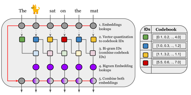
Figure 1: The N-Grammer layer. It takes as input a sequence of uni-gram embeddings and outputs a parallel sequence of N-gram augmented embeddings. The input embeddings are clustered into a discrete latent representation using PQ, and n-grams (bi-grams) IDs are computed over it. For each n-gram ID, a trainable embedding is looked up from an embedding table and combined with the input embeddings to produce the output.

2 Related Work

Memory augmented models There has been a long line of work in augmenting sequence models with memory, e.g. the Neural Turing Machine (Graves et al., 2014) and Memory Networks (Weston et al., 2014). More recent works have proposed combining Transformer based models with product key look-up tables (Lample et al., 2019), while Panigrahy et al. (2021) propose memories based on sketches of past activations. There has also been a lot of work on augmenting language models with non-parametric memory, such as the $k$-nearest neighbor language models of Khandelwal et al. (2019), and similar retrieval augmented works such as Lewis et al. (2020); Guu et al. (2020); Krishna et al. (2021). In these retrieval augmented models, the model is conditioned on documents from the training corpus or a knowledge base, with the hope that information from related articles can help improve the factual accuracy of the models.

Discrete latent models for sequences Discrete latent models using Vector Quantization (VQ) have been widely used in speech (van den Oord et al., 2017; Wang et al., 2018; Schneider et al., 2019) to learn unsupervised representations of audio signals. Their use for modeling text sequences were studied in Kaiser et al. (2018); Roy et al. (2018) where the motivation was to reduce the inference latency for neural machine translation models by decoding in the latent space.

N-gram models for statistical language modeling N-gram models have a long history in statistical modeling of language, see e.g., Brown et al. (1992, 1993); Katz (1987); Kneser and Ney (1995); Chen and Goodman (1999). Before the advent of word vectors and distributed representations of language via neural networks (Mikolov et al., 2013; Wu et al., 2016), n-gram language models were the standard in the field of statistical language modeling. More recent related work on combining neural sequence models with n-gram information is due to Sun and Iyyer (2021) who propose concatenating the representations within a local context, while Huang et al. (2021) propose combining RNN models with n-gram embedding tables. Our work differs from them in that we use an n-gram look-up table on a discrete latent representation of the sequence, which leads to a more meaningful assignment of shared n-gram representations.

Product Quantization There has also been a long line of work on investigating variants of Vector Quantization (VQ) that realize different trade-offs in data compression. The most related work in this domain is due to Jegou et al. (2011) who introduce a multi-head version of VQ which is termed Product Quantization (PQ). PQ is widely used in computer vision, see e.g., Ge et al. (2013); Yu et al. (2018). Our approach to learning discrete latent codes use PQ over the attention heads.

3 The N-Grammer layer

At a high level, we introduce a simple layer that augments the Transformer architecture with more memory based on latent n-grams. While the N-Grammer layer is general enough for considering arbitrary N-grams, we restrict ourselves to the use of bi-grams. We leave the exploration of higher-order n-grams for future work. The layer consists of four core operations:

1. Given a sequence of uni-gram embeddings of a text, infer a sequence of discrete latent representation via PQ.

2. Infer the bi-gram representation for the latent sequence.

3. Look up trainable bi-gram embeddings via hashing into the bi-gram vocabulary.

4. Combine the bi-gram embeddings with the input uni-gram embeddings.

We describe each of these operations in more detail in the following sections. To refer to a set of discrete items, we use the notation $[m]$ to mean the set $\{0,1,\cdots,m-1\}$.

3.1 Discrete latent representation of a sequence

The first step of the N-Grammer layer is to obtain a parallel sequence of discrete latent representations with Product Quantization (PQ) (Jegou et al., 2011) by learning a codebook from the given sequence of input embeddings. The input embedding is a sequence of uni-gram embeddings $x\in{\mathbb{R}^{l\times h\times d}}$, where $l$ is the length of the sequence, $h$ is the number of heads, and $d$ is the embedding dimension per head. We learn a codebook $c$ in $\mathbb{R}^{k\times h\times d}$ with $k$ code-words with mini-batch $k$-means (Bottou and Bengio, 1995), and in the same step, we form the parallel sequence of discrete latent representation $z\in[k]^{l\times h}$ of the sequence $x$ by picking the codebook IDs that have the least distance from the input embeddings:

$$z_{i,j}=\operatorname*{argmin}_{l\in[k]}\left\lVert x_{i,j}-c_{l,j}\right\rVert_{2}.$$

The advantage of this latent representation $z$ is twofold. Firstly, it makes considering all $k^{2}$ bi-grams tractable by mapping the uni-gram embeddings to share the same code-word embedding based on similarity, thereby allowing us to use a smaller bi-gram embedding table. Secondly, when using a fixed size bi-gram vocabulary, having this latent representation allows for a more efficient representation to be learned compared to directly using the uni-gram IDs. For instance, a uni-gram vocabulary of $32,000$ would entail a bi-gram vocabulary of roughly $1$ billion, which adds a significant memory overhead.

3.2 Bi-gram IDs from discrete latent representation

The second step is to convert the discrete latent representation $z$ computed in Section 3.1 to bi-gram IDs $b\in[k^{2}]^{l\times h}$. The latent bi-gram IDs are formed at each position by combining the uni-gram latent IDs $z$ from the previous position as

$$b_{i}=\begin{cases}z_{i}&\text{if $i=0$,}\\ z_{i}+kz_{i-1}&\text{otherwise}\end{cases}$$

where $k$ is the size of our codebook. This directly maps the discrete latent sequence from a vocabulary space of $[k]$ to the latent bi-gram vocabulary space of $[k^{2}]$.

3.3 Constructing bi-gram representations

The third step is to construct bi-gram latent representations $b$ of the sequence. We can consider all $k^{2}$ bi-grams and augment the model with an embedding for each such bi-gram. In practice, the compression for machine translation models with a uni-gram vocabulary of $32,000$ involves clustering each token into roughly $k=2^{12}$ clusters without sacrificing quality (Kaiser et al., 2018; Roy et al., 2018). In this instance, to consider all bi-grams would involve constructing an embedding table with $16$ million rows. Since this is still large, we map the latent bi-gram IDs to a smaller bi-gram vocabulary of size $v$, by using separate hash functions for each head.

More precisely, we have a latent bi-gram embedding table $B\in\mathbb{R}^{v\times h\times d_{b}}$, where $v$ is the bi-gram vocabulary and $d_{b}$ is the bi-gram embedding dimension. The bi-gram embedding $y\in\mathbb{R}^{l\times h\times d_{b}}$ of the text sequence is then constructed as $y_{i,j}=B\left[\left((r_{j}b_{i,j}+s_{j})\mod{p_{j}}\right)\mod{v},j\right],$ where for each head $j$, we select a random prime $p_{j}$ greater than $k^{2}$, and $r_{j}$ is chosen randomly in $\{1,\cdots,p-1\}$ and $s_{j}$ is chosen randomly in $[p-1]$. This scheme is a universal hashing scheme and guarantees a low collision probability for the discrete latent codes of each head (Thorup, 2015). Note that the bi-gram embedding vector $y_{i,j}$ is a $d_{b}$-dimensional vector.

Model	Layers	Params	Vocab size	Clusters	Dim	Inference Ex/sec	PP
Transformer	16	234M	-	-	-	402.00	15.32
Transformer-L	20	284M	-	-	-	331.12	14.70
Primer	16	234M	-	-	-	346.32	15.10
Primer-L	18	284M	-	-	-	284.40	15.01
N-Grammer	16	246M	196K	-	12.5%	379.60	15.36
N-Grammer	16	259M	196K	-	25.0%	378.64	15.27
N-Grammer	16	284M	196K	-	50.0%	375.40	15.50
N-Grammer	16	251M	196K	4K	12.5%	366.80	15.26
N-Grammer	16	263M	196K	4K	25.0%	362.40	15.07
N-Grammer	16	288M	196K	4K	50.0%	362.00	15.01
N-Grammer	16	255M	196K	8K	12.5%	359.52	15.58
N-Grammer	16	267M	196K	8K	25.0%	358.96	15.44
N-Grammer	16	292M	196K	8K	50.0%	358.16	15.01
N-Grammer	16	267M	393K	8K	12.5%	363.60	15.32
N-Grammer	16	292M	393K	8K	25.0%	360.16	15.97
N-Grammer	16	343M	393K	8K	50.0%	356.94	14.79

Table 1: Ablation results on auto-regressive language modeling on the C4 data-set (Raffel et al., 2019). The column labeled Vocab Size refers to the bi-gram vocabulary size, while the column labeled Dim refers to the bi-gram embedding dimension as a percentage of the total model dimension. All models are trained with a batch size of $256$ for a total of $1$M steps. We report the test perplexity (PP) and as well as the inference through-put in examples per second (Inference Ex/sec) on a TPU-v3 with 8 cores (higher is better).

3.4 Combining the embeddings

The final step is to form a new representation of the text sequence which is derived by combining the uni-gram embedding $x\in\mathbb{R}^{l\times h\times d}$ with the latent bi-gram embedding $y\in\mathbb{R}^{l\times h\times d_{b}}$ obtained in Section 3.3. The bi-gram embedding and uni-gram embedding are both independently layer normalized ($LN$), followed by simply concatenating the two along the embedding dimension to produce $w=[LN(x),LN(y)]\in\mathbb{R}^{l\times h\times(d+d_{b})}$ which is passed as input to rest of the Transformer network. Note that layer normalization (Ba et al., 2016) leads to more stable training.

4 Experiments & Results

We compare the N-Grammer model with the Transformer architecture (Vaswani et al., 2017) as well as with the recently proposed Primer architecture (So et al., 2021) on the C4 data-set (Raffel et al., 2019) . To establish a strong baseline for our experiments we use a Gated Linear Unit (Dauphin et al., 2017) as the feed-forward network with a GELU activation function (Hendrycks and Gimpel, 2016) in all our models, except the Primer. The Primer architecture uses a $3\times 1$ depth-wise convolution after the key, query and value projections, and the squared RELU activation function as proposed in So et al. (2021). For all experiments, we use the rotary position embedding (RoPE) from Su et al. (2021), which greatly improves the quality of all models.

We compare the N-Grammer, Primer and Transformer models in Table 1. The baseline Transformer model has $16$ layers and $8$ heads, with a model dimension of $1024$. We train all the models with a batch size of $256$ and a sequence length of $1024$ on a TPU-v3. A more detailed exposition of the various hyper-parameter choices is given in Section 5. For the N-Grammer models, we ablate with different sizes for the bi-gram embedding dimension ranging from $128$ to $512$. Since adding n-gram embeddings increases the number of trainable parameters, we also train two large baselines in Table 1 (Transformer-L and Primer-L) which have the same order of parameters as the N-Grammer models. However, unlike the larger Transformer models, the training and inference cost of N-Grammer does not scale proportional to the number of parameters in the n-gram embedding layer, since they rely on sparse look-up operations (see column Inference Ex/sec in Table 1). Thus for example, we find from Table 1 that the best N-Grammer model with a n-gram vocabulary of $393$K and a discrete latent vocabulary of $8$K matches the quality of Transformer-L and Primer-L in perplexity (14.79 vs 14.70 vs 15.01) while having significantly higher through-put (356.94 vs 331.12 vs 284.40 examples/sec).

We also examine a simple version of N-Grammer where we compute the n-grams directly from the uni-gram vocabulary as in Section 3.3 rather than from the latent representation of Section 3.1. This is reported in Table 1 and corresponds to the N-Grammer without an entry in the clusters column. Note that in this case, the modulo hashing scheme of Section 3.3 is random and independent of the content of the actual uni-gram embeddings. We inspect the individual cluster assignment in Section 10 and find common themes among the groupings.

5 Hyper-parameters for experiments

In this section we report the hyper-parameter settings for all our experiments for reproducibility purposes.

5.1 Optimizer hyper-parameters

We use the Adam optimizer (Kingma and Ba, 2015) and tune the learning rate as well as $\varepsilon$ as reported in (Agarwal et al., 2020). We find that decreasing $\varepsilon$ from the standard setting of $10^{-6}$ to $10^{-10}$ benefits the Transformer models while having less of an effect on the Primer (So et al., 2021). We use a learning rate of $10^{-3}$ for all models. We use a $\beta_{1}=0.9$ and $\beta_{2}=0.99$ and clip the gradient norm to $5.0$. We do not use any weight decay. We train all models with a global batch size of $256$ on a TPU-v3 with $32$ cores and a sequence length of $1024$.

5.2 N-Grammer hyper-parameters

For the N-Grammer models, we use a discrete latent vocabulary of $k=\{4096,8192\}$ except for the baseline N-Grammer models which directly compute n-grams on the uni-gram vocabulary. For training the n-gram embedding tables we use the Adagrad optimizer (Duchi et al., 2011), which is known to be more suitable for learning sparse features. We use a learning rate of $0.1$ for training the n-gram embedding table, with the same learning rate schedule as the base model. We find that using a $10\times$ higher or lower learning rate leads to unstable training of the N-Grammer model.

We train the cluster centers for learning the discrete latent representation using mini-batch $k$-means (Bottou and Bengio, 1995). We do not use any smoothing or exponential moving averages for either the counts or the centers, since we find empirically that it doesn’t help in our setting. We use a learning rate of $10^{-3}$ for learning the discrete representations.

6 Position of the N-Grammer layer

We perform ablation experiments on the position of the latent N-Grammer layer, since potentially one may add it to any intermediate layer of the network. We take the best N-Grammer model from Table 1, corresponding to an n-gram vocabulary size of $393$K and a latent vocabulary of size $8$K and ablate the position of the N-Grammer layer in Table 2. We observe that placing the n-gram layer at the beginning of the network turns out to be the best choice, since moving the layer successively to the end of the network leads to progressively worse performance. We hypothesize that this is due to the presence of fewer attention layers to leverage the improved representations from the $n$-gram embeddings.

Model	PP
N-Grammer	14.79
N-Grammer begin	14.92
N-Grammer mid	15.13
N-Grammer end	15.17

Table 2: Ablation results on the position of the N-Grammer layer on the C4 data-set (Raffel et al., 2019). We use the best N-Grammer model from Table 1, with a vocab size of $393$K. The N-Grammer models labelled begin, middle and end refer to the latent n-gram embedding layer being placed after the first layer, the middle layer and the end layer respectively.

7 Optimizing through-put

We note that there is a trade-off in computing the discrete latent representation of a text sequence, where it may be more efficient in practice to cluster the uni-gram vocabulary directly rather than clustering the embedded text sequence. This is an important consideration when serving the N-Grammer model, since the mapping from token to discrete latent is fixed after the completion of training thereby allowing us to pay a one time cost in computing this mapping for the entire vocabulary. We formulate this more precisely as follows.

Let the uni-gram vocabulary be $v$, the latent vocabulary $k$, the sequence length $l$, batch size $b$, and let the N-Grammer model serve a total of $m$ examples. If we were to compute the latent representation for each sequence, we incur a cost of $\mathcal{O}(bkl)$ per sequence. On the other hand, if we were to compute the latent representation for the entire vocabulary up-front and cache the mapping from token to latent, we pay a one time cost of $\mathcal{O}(vk)$ for inferring the latent representations. Assuming an $\mathcal{O}(1)$ cost of looking up the latent representation per sequence, this cost can be amortized over the $m$ examples to get a per sequence cost of $\mathcal{O}(vk/m+1)$. As $m\rightarrow\infty$, i.e., the model is continuously deployed, we essentially get to compute the discrete latent representation in constant time per sequence during serving.

Since computing the n-gram ID (see Section 3.2) and retrieving the n-gram representations are also constant (with respect to the number of attention layers, attention heads and model dimension) time operations per sequence, this implies that when served long enough, the N-Grammer model essentially incurs a constant overhead over the Transformer.

8 Convergence comparisons

We have included training curve comparisons of the N-Grammer with that of the Transformer (Vaswani et al., 2017) and the Primer (So et al., 2021). We compare the three models in Figures 2(a) and 2(b) where the $x$-axis denotes the wall clock time on a TPU-v3 while the $y$-axis denotes the log perplexity and top-1 accuracy respectively on the C4 data-set (Raffel et al., 2019). From Figure 2 we see that the N-Grammer model is roughly $2\times$ faster than the Primer in wall clock time to reach the same perplexity or accuracy. More precisely, the baseline Primer model after 1M steps (180 TPU hours) has a perplexity of $15.10$, which the best N-Grammer model from Table 1 achieves at $465$K steps (90 TPU hours).

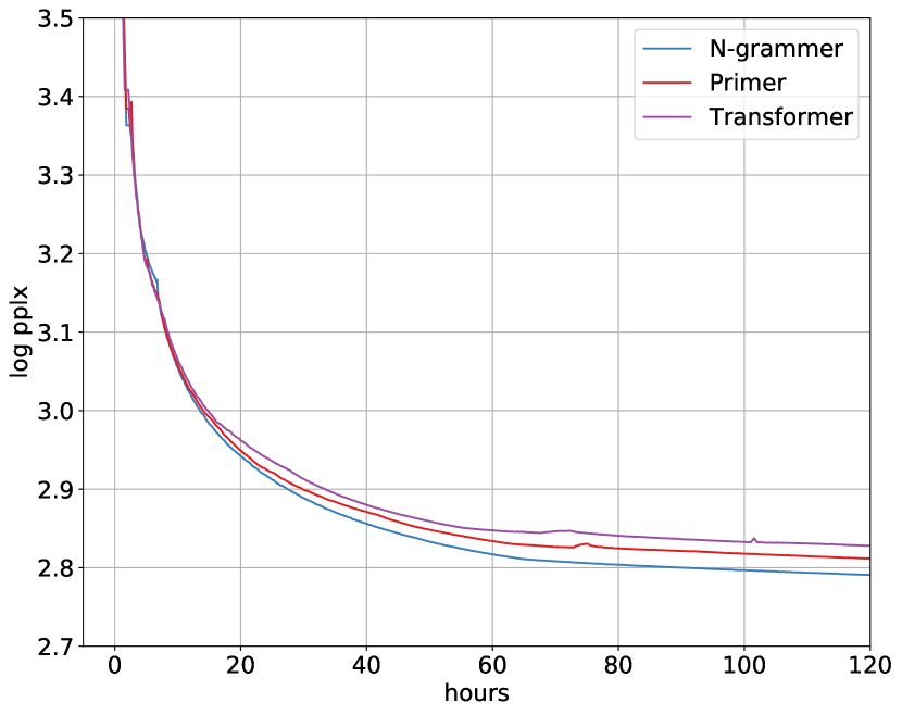
(a) Log perplexity vs wall-clock time on TPU-v3

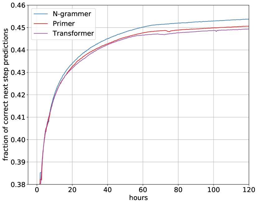
(b) Top-1 accuracy vs wall-clock time on TPU-v3

Figure 2: Wall-clock time comparisons between Transformer with Gated GELU, Primer and N-Grammer on the C4 data-set (Raffel et al., 2019).

9 Comparison on downstream tasks

We fine-tune the baseline Transformer, Primer (as well as their large variants) and the best N-Grammer model from Table 1 on the SuperGLUE benchmark (Wang et al., 2019) to evaluate whether the perplexity gains of the N-Grammer model also result in downstream classification gains. For all models we take the checkpoint at $1$M steps, and fine-tune for $100$K steps with a constant learning rate of $10^{-4}$. We report the downstream evaluation metrics in Table 3. From Table 3 we observe that the N-Grammer improves on the quality of the Transformer and Primer models on most SuperGLUE tasks. More surprisingly, we see that it also substantially improves on the larger Transformer-L and Primer-L models on tasks like COPA, RTE, WiC and WSC.

Model	BoolQ	CB	COPA	MultiRC	ReCoRD	RTE	WiC	WSC	Avg
	Acc.	F1/Acc.	Acc.	F1/EM	F1/EM	Acc.	Acc.	Acc.
Transformer	65.23	54.03/67.86	55.0	59.47/13.64	30.34/29.32	53.43	54.55	61.54	52.13
Transformer-L	66.15	73.74/75.00	59.0	62.09/12.17	29.19/28.21	57.04	55.33	62.50	55.03
Primer	66.27	62.64/71.43	53.0	62.89/12.91	30.56/29.55	55.96	54.86	65.38	53.81
Primer-L	62.20	47.69/58.93	58.0	51.83/4.62	25.21/24.35	51.99	54.08	63.46	49.50
N-Grammer	64.98	59.69/67.86	60.0	61.95/11.33	29.90/28.91	59.21	56.11	68.27	54.80

Table 3: Fine-tuning results on SuperGLUE (Wang et al., 2019) comparing the Transformer, Primer and the best N-Grammer model from Table 1. The N-Grammer model has a discrete latent vocabulary of size $8$K and a n-gram vocabulary of size $393$K. For all models we take the pre-trained checkpoint at 1M steps and fine-tune for $100$K steps with a constant learning rate of ${10}^{-4}$.

10 Analysis of the latent representations

We inspect the discrete latent representations learned by the N-Grammer layer by examining the different uni-gram tokens that are assigned to the same cluster ID. We take a trained N-Grammer model with $8192$ clusters, n-gram embedding dimension of $16$ and n-gram vocabulary of 196K. We pass the entire set of $32,000$ uni-gram embeddings as input to the N-Grammer layer, thereby gathering the cluster assignment of every uni-gram token. We present some of these in Table 4, where we find that the model learns to group related uni-gram tokens together:

1. the cluster with head ID $0$ and cluster ID $6259$ corresponds to sports and games,

2. the cluster with head ID $2$ and cluster ID $5362$ corresponds to places,

3. the cluster with head ID $0$ and cluster ID $7468$ corresponds to animals and fruits,

4. the cluster with head ID $2$ and cluster ID $8080$ corresponds to the arts,

5. the cluster with head ID $4$ and cluster ID $6618$ also corresponds to the arts.

We also observe that several heads independently learn a similar themed grouping, e.g., head $2$ and $4$ both have a cluster dedicated to arts and entertainment.

Head ID	Cluster ID	Uni-gram Tokens
0	6259	Baseball, football, ceramic, Galaxy, hockey, basketball, Cricket, Basketball, guitar, acquisition, athlete, Soccer, Squid, sports
2	5362	Alchemist, Vegas, hanger, Seinfeld, Kenya, Heroic, Kurdish, Rodgers, Bolivia, Venom, Qatar, dosage, Arcade, Emperor, becua, Finnish, Taiwanese, Chennai, hood, dub, flake, Balkan, Psalm, Bueno, Moldova, flow, mosquito, Filipino, Throne, Siberia, Trout, Fist, Czech, Boulevard, Azerbaijan, Peru, OW, plaster, Kashmir, NZ, Priest, Palestinian, Tibetan, stencil, Aragon, coils, HBO, Iceland, strains, Zimbabwe, firewall, Nepal, Elves, Iranian, Mongol, Traffic, Camilla, parade, Afghan, hose, Serpent, Tarantino, web, Khal, Squid, Mala, Syrian, hood
0	7468	Unknown, spoon, Shut, coconut, grapefruit, cran, Kami, moon, spider, yogurt, perfume, Wine, Skate, antique, snail, Onion, guinea, puppy, mineral, Reagan, elbow, bark, patio, beneath, snake, lever, bunny, falcon, rail, ribbon, knob, apples, quarry, corn, nach, hiking, invoice, Pour, flora, fishing, Paint, olive, violin, octopus, horizontal, blanket, circular, army, nickel, cattle, potato, dolphin, mosquito, citrus, shutter
2	8080	Knicks, Shakespeare, SPE, nursing, spells, Alexa, arrow, vocalist, rehearsal, tunnel, eine, Critical, clar, BAN, remix, obstacle, musicians, BRO, legislature, EMS, Manga, piano, sword, vocal, bald, choir, Messi, Beta, cad, illustrator, organ, conjunction, lunar, bien, needles, musician, hiking, tad, poe, Pay, violin, Marxist, literary, Theater, gig, poetry, Illustrator, guitar, Pluto, Camaro, Fog, orbit, dancing, epub
4	6618	Wise, vocalist, actor, cheek, musicians, TION, piano, tunes, choir, filmmaker, musician, Suzuki, violin, Theater, gig, Drama, guitar, logic, Entertainment

Table 4: Mapping of uni-gram tokens to cluster IDs for the N-Grammer model. The N-Grammer model has $8$ heads, $8192$ clusters, an n-gram embedding dimension of 16 and a n-gram vocabulary of 196K. We report the head index (Head ID), the cluster index (Cluster ID) and the uni-gram tokens assigned to those IDs for a random subset of clusters.

11 Conclusion

We introduced the N-Grammer layer for augmenting the Transformer architecture with latent n-grams, and find that it can match a larger Transformer and Primer in quality while being significantly faster in inference. The N-Grammer architecture is particularly suitable for devices that allow storing large embedding tables while supporting only distributed gather-scatter operations. We also showed that by caching the mapping from token to discrete latent, one can serve the N-Grammer architecture with only a constant overhead over the Transformer. This makes the N-Grammer attractive for deployment, since on most hardware platforms sparse operations such as an embedding look-up is significantly faster than dense operations such as matrix multiplications.

References

- Agarwal et al. (2020) Naman Agarwal, Rohan Anil, Elad Hazan, Tomer Koren, and Cyril Zhang. 2020. Disentangling adaptive gradient methods from learning rates. arXiv preprint arXiv:2002.11803.
- Ainslie et al. (2020) Joshua Ainslie, Santiago Ontanon, Chris Alberti, Vaclav Cvicek, Zachary Fisher, Philip Pham, Anirudh Ravula, Sumit Sanghai, Qifan Wang, and Li Yang. 2020. Etc: Encoding long and structured inputs in transformers. arXiv preprint arXiv:2004.08483.
- Ba et al. (2016) Jimmy Lei Ba, Jamie Ryan Kiros, and Geoffrey E Hinton. 2016. Layer normalization. arXiv preprint arXiv:1607.06450.
- Bahdanau et al. (2015) Dzmitry Bahdanau, Kyunghyun Cho, and Yoshua Bengio. 2015. Neural machine translation by jointly learning to align and translate. In 3rd International Conference on Learning Representations, ICLR 2015.
- Bottou and Bengio (1995) Leon Bottou and Yoshua Bengio. 1995. Convergence properties of the k-means algorithms. In Advances in neural information processing systems, pages 585–592.
- Brown et al. (1993) Peter F Brown, Stephen A Della Pietra, Vincent J Della Pietra, and Robert L Mercer. 1993. The mathematics of statistical machine translation: Parameter estimation. Computational linguistics, 19(2):263–311.
- Brown et al. (1992) Peter F Brown, Vincent J Della Pietra, Peter V Desouza, Jennifer C Lai, and Robert L Mercer. 1992. Class-based n-gram models of natural language. Computational linguistics, 18(4):467–480.
- Brown et al. (2020) Tom B Brown, Benjamin Mann, Nick Ryder, Melanie Subbiah, Jared Kaplan, Prafulla Dhariwal, Arvind Neelakantan, Pranav Shyam, Girish Sastry, Amanda Askell, et al. 2020. Language models are few-shot learners. arXiv preprint arXiv:2005.14165.
- Chen and Goodman (1999) Stanley F Chen and Joshua Goodman. 1999. An empirical study of smoothing techniques for language modeling. Computer Speech & Language, 13(4):359–394.
- Cho et al. (2014) Kyunghyun Cho, Bart van Merriënboer, Caglar Gulcehre, Dzmitry Bahdanau, Fethi Bougares, Holger Schwenk, and Yoshua Bengio. 2014. Learning phrase representations using rnn encoder–decoder for statistical machine translation. In Proceedings of the 2014 Conference on Empirical Methods in Natural Language Processing (EMNLP), pages 1724–1734.
- Correia et al. (2019) Gonçalo M Correia, Vlad Niculae, and André FT Martins. 2019. Adaptively sparse transformers. arXiv preprint arXiv:1909.00015.
- Dauphin et al. (2017) Yann N Dauphin, Angela Fan, Michael Auli, and David Grangier. 2017. Language modeling with gated convolutional networks. In International conference on machine learning, pages 933–941. PMLR.
- Devlin et al. (2019) Jacob Devlin, Ming-Wei Chang, Kenton Lee, and Kristina Toutanova. 2019. Bert: Pre-training of deep bidirectional transformers for language understanding. In NAACL-HLT (1).
- Duchi et al. (2011) John Duchi, Elad Hazan, and Yoram Singer. 2011. Adaptive subgradient methods for online learning and stochastic optimization. Journal of machine learning research, 12(7).
- Fedus et al. (2021) William Fedus, Barret Zoph, and Noam Shazeer. 2021. Switch transformers: Scaling to trillion parameter models with simple and efficient sparsity. arXiv preprint arXiv:2101.03961.
- Ge et al. (2013) Tiezheng Ge, Kaiming He, Qifa Ke, and Jian Sun. 2013. Optimized product quantization for approximate nearest neighbor search. In Proceedings of the IEEE Conference on Computer Vision and Pattern Recognition, pages 2946–2953.
- Graves et al. (2014) Alex Graves, Greg Wayne, and Ivo Danihelka. 2014. Neural turing machines. arXiv preprint arXiv:1410.5401.
- Guu et al. (2020) Kelvin Guu, Kenton Lee, Zora Tung, Panupong Pasupat, and Ming-Wei Chang. 2020. Realm: Retrieval-augmented language model pre-training. arXiv preprint arXiv:2002.08909.
- Hendrycks and Gimpel (2016) Dan Hendrycks and Kevin Gimpel. 2016. Gaussian error linear units (gelus). arXiv preprint arXiv:1606.08415.
- Huang et al. (2021) W Ronny Huang, Tara N Sainath, Cal Peyser, Shankar Kumar, David Rybach, and Trevor Strohman. 2021. Lookup-table recurrent language models for long tail speech recognition. arXiv preprint arXiv:2104.04552.
- Jegou et al. (2011) Herve Jegou, Matthijs Douze, and Cordelia Schmid. 2011. Product quantization for nearest neighbor search. IEEE transactions on pattern analysis and machine intelligence, 33(1):117–128.
- Kaiser et al. (2018) Łukasz Kaiser, Aurko Roy, Ashish Vaswani, Niki Pamar, Samy Bengio, Jakob Uszkoreit, and Noam Shazeer. 2018. Fast decoding in sequence models using discrete latent variables. arXiv preprint arXiv:1803.03382.
- Katz (1987) Slava Katz. 1987. Estimation of probabilities from sparse data for the language model component of a speech recognizer. IEEE transactions on acoustics, speech, and signal processing, 35(3):400–401.
- Khandelwal et al. (2019) Urvashi Khandelwal, Omer Levy, Dan Jurafsky, Luke Zettlemoyer, and Mike Lewis. 2019. Generalization through memorization: Nearest neighbor language models. arXiv preprint arXiv:1911.00172.
- Kingma and Ba (2015) Diederik P. Kingma and Jimmy Ba. 2015. Adam: A method for stochastic optimization. In 3rd International Conference on Learning Representations, ICLR 2015, San Diego, CA, USA, May 7-9, 2015, Conference Track Proceedings.
- Kneser and Ney (1995) Reinhard Kneser and Hermann Ney. 1995. Improved backing-off for m-gram language modeling. In 1995 international conference on acoustics, speech, and signal processing, volume 1, pages 181–184. IEEE.
- Koehn (2009) Philipp Koehn. 2009. Statistical machine translation. Cambridge University Press.
- Krishna et al. (2021) Kalpesh Krishna, Aurko Roy, and Mohit Iyyer. 2021. Hurdles to progress in long-form question answering. arXiv preprint arXiv:2103.06332.
- Lample et al. (2019) Guillaume Lample, Alexandre Sablayrolles, Marc’Aurelio Ranzato, Ludovic Denoyer, and Hervé Jégou. 2019. Large memory layers with product keys. arXiv preprint arXiv:1907.05242.
- Lepikhin et al. (2020) Dmitry Lepikhin, HyoukJoong Lee, Yuanzhong Xu, Dehao Chen, Orhan Firat, Yanping Huang, Maxim Krikun, Noam Shazeer, and Zhifeng Chen. 2020. Gshard: Scaling giant models with conditional computation and automatic sharding. arXiv preprint arXiv:2006.16668.
- Lewis et al. (2020) Patrick Lewis, Ethan Perez, Aleksandra Piktus, Fabio Petroni, Vladimir Karpukhin, Naman Goyal, Heinrich Küttler, Mike Lewis, Wen-tau Yih, Tim Rocktäschel, et al. 2020. Retrieval-augmented generation for knowledge-intensive nlp tasks. arXiv preprint arXiv:2005.11401.
- Mikolov et al. (2013) Tomas Mikolov, Kai Chen, Greg Corrado, and Jeffrey Dean. 2013. Efficient estimation of word representations in vector space. arXiv preprint arXiv:1301.3781.
- Panigrahy et al. (2021) Rina Panigrahy, Xin Wang, and Manzil Zaheer. 2021. Sketch based memory for neural networks. In International Conference on Artificial Intelligence and Statistics, pages 3169–3177. PMLR.
- Radford et al. (2018) Alec Radford, Karthik Narasimhan, Tim Salimans, and Ilya Sutskever. 2018. Improving language understanding by generative pre-training. URL https://s3-us-west-2. amazonaws. com/openai-assets/research-covers/languageunsupervised/language understanding paper. pdf.
- Raffel et al. (2019) Colin Raffel, Noam Shazeer, Adam Roberts, Katherine Lee, Sharan Narang, Michael Matena, Yanqi Zhou, Wei Li, and Peter J Liu. 2019. Exploring the limits of transfer learning with a unified text-to-text transformer. arXiv preprint arXiv:1910.10683.
- Roy et al. (2021) Aurko Roy, Mohammad Saffar, Ashish Vaswani, and David Grangier. 2021. Efficient content-based sparse attention with routing transformers. Transactions of the Association for Computational Linguistics, 9:53–68.
- Roy et al. (2018) Aurko Roy, Ashish Vaswani, Arvind Neelakantan, and Niki Parmar. 2018. Theory and experiments on vector quantized autoencoders. arXiv preprint arXiv:1805.11063.
- Schneider et al. (2019) Steffen Schneider, Alexei Baevski, Ronan Collobert, and Michael Auli. 2019. wav2vec: Unsupervised pre-training for speech recognition. arXiv preprint arXiv:1904.05862.
- Shazeer et al. (2017) Noam Shazeer, Azalia Mirhoseini, Krzysztof Maziarz, Andy Davis, Quoc Le, Geoffrey Hinton, and Jeff Dean. 2017. Outrageously large neural networks: The sparsely-gated mixture-of-experts layer. arXiv preprint arXiv:1701.06538.
- So et al. (2021) David R So, Wojciech Mańke, Hanxiao Liu, Zihang Dai, Noam Shazeer, and Quoc V Le. 2021. Primer: Searching for efficient transformers for language modeling. arXiv preprint arXiv:2109.08668.
- Su et al. (2021) Jianlin Su, Yu Lu, Shengfeng Pan, Bo Wen, and Yunfeng Liu. 2021. Roformer: Enhanced transformer with rotary position embedding. arXiv preprint arXiv:2104.09864.
- Sun and Iyyer (2021) Simeng Sun and Mohit Iyyer. 2021. Revisiting simple neural probabilistic language models. arXiv preprint arXiv:2104.03474.
- Thorup (2015) Mikkel Thorup. 2015. High speed hashing for integers and strings. arXiv preprint arXiv:1504.06804.
- van den Oord et al. (2017) Aäron van den Oord, Oriol Vinyals, and Koray Kavukcuoglu. 2017. Neural discrete representation learning. CoRR, abs/1711.00937.
- Vaswani et al. (2017) Ashish Vaswani, Noam Shazeer, Niki Parmar, Jakob Uszkoreit, Llion Jones, Aidan N Gomez, Łukasz Kaiser, and Illia Polosukhin. 2017. Attention is all you need. In Advances in neural information processing systems, pages 5998–6008.
- Wang et al. (2019) Alex Wang, Yada Pruksachatkun, Nikita Nangia, Amanpreet Singh, Julian Michael, Felix Hill, Omer Levy, and Samuel Bowman. 2019. Superglue: A stickier benchmark for general-purpose language understanding systems. Advances in neural information processing systems, 32.
- Wang et al. (2018) Yuxuan Wang, Daisy Stanton, Yu Zhang, RJ-Skerry Ryan, Eric Battenberg, Joel Shor, Ying Xiao, Ye Jia, Fei Ren, and Rif A Saurous. 2018. Style tokens: Unsupervised style modeling, control and transfer in end-to-end speech synthesis. In International Conference on Machine Learning, pages 5180–5189. PMLR.
- Weston et al. (2014) Jason Weston, Sumit Chopra, and Antoine Bordes. 2014. Memory networks. arXiv preprint arXiv:1410.3916.
- Wu et al. (2021) Haiping Wu, Bin Xiao, Noel Codella, Mengchen Liu, Xiyang Dai, Lu Yuan, and Lei Zhang. 2021. Cvt: Introducing convolutions to vision transformers. arXiv preprint arXiv:2103.15808.
- Wu et al. (2016) Yonghui Wu, Mike Schuster, Zhifeng Chen, Quoc V Le, Mohammad Norouzi, Wolfgang Macherey, Maxim Krikun, Yuan Cao, Qin Gao, Klaus Macherey, et al. 2016. Google’s neural machine translation system: Bridging the gap between human and machine translation. arXiv preprint arXiv:1609.08144.
- Yu et al. (2018) Tan Yu, Junsong Yuan, Chen Fang, and Hailin Jin. 2018. Product quantization network for fast image retrieval. In Proceedings of the European Conference on Computer Vision (ECCV), pages 186–201.
- Zaheer et al. (2020) Manzil Zaheer, Guru Guruganesh, Kumar Avinava Dubey, Joshua Ainslie, Chris Alberti, Santiago Ontanon, Philip Pham, Anirudh Ravula, Qifan Wang, Li Yang, et al. 2020. Big bird: Transformers for longer sequences. In NeurIPS.