BR-SNIS: Bias Reduced Self-Normalized Importance Sampling

Abstract

Importance Sampling (IS) is a method for approximating expectations under a target distribution using independent samples from a proposal distribution and the associated importance weights. In many applications, the target distribution is known only up to a normalization constant, in which case self-normalized IS (SNIS) can be used. While the use of self-normalization can have a positive effect on the dispersion of the estimator, it introduces bias. In this work, we propose a new method, BR-SNIS, whose complexity is essentially the same as that of SNIS and which significantly reduces bias without increasing the variance. This method is a wrapper in the sense that it uses the same proposal samples and importance weights as SNIS, but makes clever use of iterated sampling–importance resampling (i-SIR) to form a bias-reduced version of the estimator. We furnish the proposed algorithm with rigorous theoretical results, including new bias, variance and high-probability bounds, and these are illustrated by numerical examples.

1 Introduction

Background and previous work:

Importance sampling [15, 1] (IS) is a classical Monte Carlo technique for estimating expectations under some given probability distribution (the target) on the basis of a sample of draws from a different distribution (the proposal). In the modern era of artificial intelligence and statistical machine learning, characterized by large computational resources and Bayesian inference, IS technologies are enjoying a revival; see, e.g., [34, 20] and [11] for a recent survey. The method is not only relevant to situations where sampling from the target is intractable; it can also be used to achieve variance reduction [21]. When the proposal is dominating the target—in the sense that the support of the latter is contained in the support of the former—unbiased estimation can be achieved by assigning each draw an importance weight given by the likelihood ratio between the target and the proposal. In the very common case where the target is known only up to a normalizing constant, consistent estimation can still be achieved by simply normalizing each importance weight by the total weight of the sample; however, since such self-normalized importance sampling (SNIS) involves ratios of random variables, the procedure can only be implemented at the cost of bias, which can be significant in some applications.

More precisely, let $(\mathbbm{X},\mathcal{X})$ be some state space and $\pi(\mathrm{d}x)\propto w(x)\lambda(\mathrm{d}x)$ a given target probability distribution, where $w$ and $\lambda$ are a positive weight function and a proposal probability distribution on $(\mathbbm{X},\mathcal{X})$, respectively, such that the normalizing constant $\lambda(w)=\int w(x)\lambda(\mathrm{d}x)$ (this will be our generic notation for Lebesgue integrals) of $\pi$ is finite. The SNIS estimator is given by

$${\textstyle\Pi_{M}f(X^{1:M})=\sum_{i=1}^{M}\omega_{M}^{i}f(X^{i}),\qquad\omega_{M}^{i}=w(X^{i})/\sum_{\ell=1}^{M}w(X^{\ell})}$$ (1)

where $X^{1:M}=(X^{1},\ldots,X^{M})$ are independent draws from $\lambda$, and can be used to approximate $\pi(f)=\int f(x)\pi(\mathrm{d}x)$ for any test function $f$ such that $\pi(|f|)<\infty$. The estimator (1) can be calculated without knowledge of the normalizing constant $\lambda(w)$, which is intractable in general.

The SNIS estimator is known to be biased; provided that $\lambda(w^{2})<\infty$, the bias and mean-squared error (MSE) of the SNIS estimator (1) over bounded test functions $f$ satisfying $\|f\|_{\infty}\leq 1$ are given respectively (see [1, Theorem 2.1]) by

$$|\mathbb{E}[\Pi_{M}f(X^{1:M})]-\pi(f)|\leq(12/M)\kappa[\pi,\lambda],\quad\mathbb{E}[\{\Pi_{M}f(X^{1:M})-\pi(f)\}^{2}]\leq(4/M)\kappa[\pi,\lambda],$$ (2)

where $\kappa[\pi,\lambda]=\lambda(w^{2})/\lambda^{2}(w)$. Although IS is primarily intended to approximate integrals in the form $\pi(f)$, it can also be used to generate unweighted samples being approximately distributed according to $\pi$. In this paper, we consider iterated sampling importance resampling (i-SIR), proposed in [42]; see [4, 24, 23, 5]. The i-SIR can be seen as an iterative application of the sampling importance resampling (SISR) algorithm proposed by [37]; the $k$-th iteration is defined as follows. Given a state $Y_{k}\in\mathbbm{X}$, (i) set $X^{1}_{k+1}=Y_{k}$ and draw $X_{k+1}^{2:N}$ independently from the proposal distribution $\lambda$; (ii) compute, for $i\in\{1,\dots,N\}$, the normalized importance weights $\omega^{i}_{N,k+1}=w(X^{i}_{k+1})/\sum_{\ell=1}^{N}w(X^{\ell}_{k+1})$; (iii) select $Y_{k+1}$ from the set $X_{k+1}^{1:N}$ by choosing $X_{k+1}^{i}$ with probability $\omega^{i}_{N,k+1}$. In the following, $Y_{k+1}$ and $X_{k+1}^{1:N}$ will be referred to as the state and the candidate pool, respectively. Following [42] (see Section 2.1), i-SIR may be viewed (up to an irrelevant permutation of the samples) as a two-stage Gibbs sampler targeting an extended probability distribution $\boldsymbol{\varphi}_{N}$ on an enlarged state space including the state as well as the candidate pool. As this extended distribution allows $\pi$ as a marginal with respect to the state, one can expect the marginal distribution of the generated states $(Y_{k})_{k\in\mathbb{N}}$, forming themselves a Markov chain, to approach the target $\pi$ of interest as $k$ tends to infinity.

This paper:

In i-SIR, the only function of the candidate pool is to guide the states selected at stage (iii) towards the target. Thus, since all rejected candidates are discarded, the approach results generally in a large waste of computational work. Thus, in the present paper we propose to recycle all the generated samples by incorporating all the proposed candidates $X_{k}^{1:N}$ into the estimator rather than only the selected candidate $Y_{k}$. We proceed in three steps. First, we show that under the stationary distribution $\boldsymbol{\varphi}_{N}$ of the process $(Y_{k},X_{k}^{1:N})_{k\in\mathbb{N}}$ generated by i-SIR, the expectation of $\Pi_{N}f(X_{k}^{1:N})$ (given by (1)) equals $\pi(f)$ for every valid test function $f$ (see Theorem 2). Second, we establish that since i-SIR is nothing but a systematic-scan Gibbs sampler, the two processes $(X_{k}^{1:N})_{k\in\mathbb{N}}$ and $(Y_{k})_{k\in\mathbb{N}}$ are interleaving (see Theorem 5); thus, if $(Y_{k})_{k\in\mathbb{N}}$ is uniformly geometrically ergodic, so is $(X_{k}^{1:N})_{k\in\mathbb{N}}$ with the same mixing rate $\kappa_{N}$. Third, as the main result of the present paper, we establish a novel $\mathcal{O}(\kappa_{N}^{k}/N)$ bound on the bias of the estimator $\Pi_{N}f(X_{k}^{1:N})$ (see Theorem 3), where the exponentially diminishing factor $\kappa_{N}^{k}$ indicates a drastic bias reduction vis-à-vis the standard IS estimator (1) based on i.i.d. samples. As a consequence, approximating $\pi(f)$ by the average of $(\Pi_{N}f(X_{k}^{1:N}))_{\ell=k_{0}+1}^{k}$, where the “burn-in” period $k_{0}$ should be chosen proportionally to the mixing time of the process, yields an estimator whose bias can be furnished with a bound which is, roughly, proportional to $\kappa_{N}^{k_{0}}$ and inversely proportional to the total number $M=kN$ of samples generated in the algorithm (see Theorem 4). To complete the theoretical analysis of these estimators, we also equip the same with variance bounds. The procedure of recycling, as described above, all the samples generated in the i-SIR and to incorporate, at negligible computational cost, the same into the final estimator, will from now on be referred as BR-SNIS. Finally, we test numerically the proposed estimators and illustrate how a significant bias reduction relatively to the standard i-SIR can be obtained at basically no cost.

To sum up, our contribution is twofold, since we

• propose a new algorithm, BR-SNIS, which makes better use of the available computational resources by recycling the candidate pool generated at each iteration of i-SIR.

• furnish the proposed algorithm with rigorous theoretical results, including novel bias, variance, and high-probability bounds which support our claim that sample recycling may lead to drastic bias reduction without impairing the variance.

2 Main results

2.1 Statements

The i-SIR algorithm can be interpreted as a systematic-scan two-stage Gibbs sampler, alternately sampling from the full conditions of an extended target $\boldsymbol{\varphi}_{N}$ on the product space of states and candidate pools. Once the extended target $\boldsymbol{\varphi}_{N}$ is properly defined, these full conditionals can be retrieved from a dual representation of $\boldsymbol{\varphi}_{N}$ presented in Theorem 1. In order to define $\boldsymbol{\varphi}_{N}$, we introduce the Markov kernel (see Section A.1 for comments)

$${\textstyle\boldsymbol{\Lambda}_{N}(y,\mathrm{d}x^{1:N})=N^{-1}\sum\nolimits_{i=1}^{N}\delta_{y}(\mathrm{d}x^{i})\prod\nolimits_{j\neq i}\lambda(\mathrm{d}x^{j})}$$ (3)

on $\mathbbm{X}\times\mathcal{X}^{\varotimes N}$, which describes probabilistically the sampling operation (i) in i-SIR. Using the kernel $\boldsymbol{\Lambda}_{N}$ we may now define properly the extended target $\boldsymbol{\varphi}_{N}$ as the probability law

$${\textstyle\boldsymbol{\varphi}_{N}(\mathrm{d}(y,x^{1:N}))=\pi(\mathrm{d}y)\boldsymbol{\Lambda}_{N}(y,\mathrm{d}x^{1:N})=N^{-1}\sum_{i=1}^{N}\pi(\mathrm{d}y)\delta_{y}(\mathrm{d}x^{i})\prod_{j\neq i}\lambda(\mathrm{d}x^{j})}$$ (4)

on $(\mathbbm{X}^{N+1},\mathcal{X}^{\varotimes(N+1)})$. Note that since for every $A\in\mathcal{X}$, $\boldsymbol{\varphi}_{N}(\mathds{1}_{A\times\mathbbm{X}^{N}})=\pi(A)$, the target $\pi$ coincides with the marginal of $\boldsymbol{\varphi}_{N}$ with respect to the state. Moreover, it is easily seen that $\boldsymbol{\Lambda}_{N}$ provides the conditional distribution, under $\boldsymbol{\varphi}_{N}$, of the candidate pool given the state. Defining the kernels

$${\textstyle\Gamma_{N}(x^{1:N},\mathrm{d}y)=N^{-1}\sum_{i=1}^{N}w(x^{i})\delta_{x^{i}}(\mathrm{d}y),\quad\Pi_{N}(x^{1:N},\mathrm{d}y)={\Gamma_{N}(x^{1:N},\mathrm{d}y)}/{\Gamma_{N}\mathds{1}_{\mathbbm{X}}(x^{1:N})}}$$ (5)

on $\mathbbm{X}\times\mathcal{X}^{\varotimes N}$, the marginal distribution $\boldsymbol{\pi}_{N}$ of $\boldsymbol{\varphi}_{N}$ with respect to $x^{1:N}$ is given by

$${\textstyle\boldsymbol{\pi}_{N}(\mathrm{d}x^{1:N})={\lambda(w)}^{-1}\Gamma_{N}\mathds{1}_{\mathbbm{X}}(x^{1:N})\prod_{j=1}^{N}\lambda(\mathrm{d}x^{j}).}$$ (6)

It is interesting to note that the marginal $\boldsymbol{\pi}_{N}$ has a probability density function, proportional to $\Gamma_{N}\mathds{1}_{\mathbbm{X}}(x^{1:N})=\sum_{i=1}^{N}w(x^{i})/N$, with respect to the product measure $\lambda^{\varotimes N}$. Using (6), we immediately obtain the following result.

Theorem 1 (duality of extended target).

For every $N\in\mathbb{N}^{*}$,

$$\boldsymbol{\varphi}_{N}(\mathrm{d}(y,x^{1:N}))=\pi(\mathrm{d}y)\boldsymbol{\Lambda}_{N}(y,\mathrm{d}x^{1:N})=\boldsymbol{\pi}_{N}(\mathrm{d}x^{1:N})\Pi_{N}(x^{1:N},\mathrm{d}y).$$ (7)

Note that the second identity of the dual representation (7) provides also the conditional distribution, under $\boldsymbol{\varphi}_{N}$, of the state given the candidates. Consequently, i-SIR is a systematic scan two-stage Gibbs sampler which generates a Markov chain $(X_{k},Y_{k})_{{k}\in\mathbb{N}}$ with time-homogeneous Markov kernel

$$\mathsf{\mathbf{P}}_{N}((y_{k},x_{k}^{1:N}),\mathrm{d}(y_{{k}+1},x_{{k}+1}^{1:N}))=\boldsymbol{\Lambda}_{N}(y_{k},\mathrm{d}x_{{k}+1}^{1:N})\Pi_{N}(x_{{k}+1}^{1:N},\mathrm{d}y_{{k}+1})$$ (8)

on $\mathbbm{X}^{N+1}\times\mathcal{X}^{\varotimes(N+1)}$. Note that the law $\mathsf{\mathbf{P}}_{N}(y_{k},x_{k}^{1:N},\cdot)$ does not depend on $x_{k}^{1:N}$, which means that only the state $Y_{k}$ needs to be stored from one iteration to the other. Thus, $(Y_{k})_{k\in\mathbb{N}}$ is a Markov chain with Markov transition kernel

$${\textstyle\mathsf{P}_{N}(y_{k},\mathrm{d}y_{k+1})=\int\boldsymbol{\Lambda}_{N}(y_{k},\mathrm{d}x_{{k}+1}^{1:N})\Pi_{N}(x_{{k}+1}^{1:N},\mathrm{d}y_{{k}+1})=\boldsymbol{\Lambda}_{N}\Pi_{N}}(y_{k},\mathrm{d}y_{k+1})$$ (9)

(where integration is w.r.t. $x_{{k}+1}^{1:N}$) on $\mathbbm{X}\times\mathcal{X}$. Given some probability distribution ${\boldsymbol{\xi}}$ on $(\mathbbm{X}^{N+1},\mathcal{X}^{\varotimes(N+1)})$, we denote by $\mathbb{P}_{\boldsymbol{\xi}}$ the law of the canonical Markov chain $(X_{k},Y_{k})_{{k}\in\mathbb{N}}$ with kernel $\mathsf{\mathbf{P}}_{N}$ and initial distribution ${\boldsymbol{\xi}}$. Our first results establishes the unbiasedness of the estimator $\Pi_{N}f(X^{1:N})$ under $\boldsymbol{\varphi}_{N}$.

Theorem 2.

For every $N\in\mathbb{N}^{*}$ and $\pi$-integrable function $f$,

$${\textstyle\int\Pi_{N}f(x^{1:N})\boldsymbol{\pi}_{N}(\mathrm{d}x^{1:N})=\pi(f).}$$

The proof of Theorem 2 is postponed to Section A.3. Next, we present theoretical bounds on the discrepancy, in terms of bias, MSE and covariance, between $\Pi_{N}f(X_{k}^{1:N})$ and $\pi(f)$, for bounded target functions $f$, when the i-SIR chain is initialized according to an arbitrary distribution ${\boldsymbol{\xi}}$. We will work under the following assumption.

A 1.

It holds that $\omega=\|w\|_{\infty}/\lambda(w)<\infty$.

Under A 1, the state and candidate-pool Markov chains $(Y_{k})_{k\in\mathbb{N}}$ and $(X^{1:N})_{k\in\mathbb{N}}$ can be shown to be uniformly geometrically ergodic with mixing rate and mixing-time upper bound

$$\kappa_{N}=(2\omega-1)/(2\omega+N-2),\quad\tau_{\scriptsize{\mbox{{\it mix}}},N}=\lceil-\ln 4/\ln\kappa_{N}\rceil,$$ (10)

respectively; see Theorem 6 below for details. Here the mixing time $\tau_{\scriptsize{\mbox{{\it mix}}},N}$ grows logarithmically with the sample size $N$. The exact value of $\tau_{\scriptsize{\mbox{{\it mix}}},N}$ is likely to be grossly pessimistic, but we conjecture that the logarithmic dependence in the minibatch size holds true. In addition, under A 1 we define the constants

$$\begin{split}\varsigma^{\scriptsize{\mbox{{\it bias}}}}&=4(\kappa[\pi,\lambda]+1+\omega)\\ \varsigma^{\scriptsize{\mbox{{\it mse}}}}_{i}&=4(\kappa[\pi,\lambda]\mathds{1}_{\{0,1\}}(i)+(1+\omega)^{2}\mathds{1}_{\{1,2\}}(i)),\quad\varsigma^{\scriptsize{\mbox{{\it cov}}}}_{i}=\varsigma^{\scriptsize{\mbox{{\it bias}}}}(\varsigma^{\scriptsize{\mbox{{\it mse}}}}_{i})^{1/2},\quad i\in\{0,1,2\}.\end{split}$$ (11)

With these definitions, the following holds true.

Theorem 3.

Assume A 1. Then for every initial distribution ${\boldsymbol{\xi}}$ on $(\mathbbm{X}^{N+1},\mathcal{X}^{\varotimes(N+1)})$, bounded measurable function $f$ on $(\mathbbm{X},\mathcal{X})$ such that $\|f\|_{\infty}\leq 1$, $N\geq 2$, and $({k},\ell)\in(\mathbb{N}^{*})^{2}$,

1. $\left|\mathbb{E}_{{\boldsymbol{\xi}}}[\Pi_{N}f(X_{k}^{1:N})]-\pi(f)\right|\leq\varsigma^{\scriptsize{\mbox{{\it bias}}}}(N-1)^{-1}\kappa_{N}^{{k}-1}$,

2. $\mathbb{E}_{{\boldsymbol{\xi}}}[\{\Pi_{N}f(X_{k}^{1:N})-\pi(f)\}^{2}]\leq\sum_{i=0}^{2}\varsigma^{\scriptsize{\mbox{{\it mse}}}}_{i}(N-1)^{-1-i/2}$,

3. $\left|\mathbb{E}_{{\boldsymbol{\xi}}}[\{\Pi_{N}f(X_{k}^{1:N})-\pi(f)\}\{\Pi_{N}f(X_{{k}+\ell}^{1:N})-\pi(f)\}]\right|\leq\kappa_{N}^{\ell-1}\sum_{i=0}^{2}\varsigma^{\scriptsize{\mbox{{\it cov}}}}_{i}(N-1)^{-(3-i/2)/2}$,

where constants are given in (10) and (11).

It is worth noting that the bias decreases inversely with the number of candidates and exponentially with the number of iterations (the mixing time of the chain also depends on $N$). The MSE is also inversely proportional to the number of candidates $N$. In the light of the previous results, it is natural to consider an estimator formed by an average across the IS estimators $(\Pi_{N}f(X_{k}^{1:N}))_{{k}\in\mathbb{N}}$ associated with the candidate pools generated at the different i-SIR iterations. To mitigate the bias, we remove a “burn-in” period whose length ${k}_{0}$ should be chosen proportional to the mixing time $\tau_{\scriptsize{\mbox{{\it mix}}},N}$ of the Markov chain $(Y_{{k}})_{{k}\in\mathbb{N}}$ (which turns out to coincide with that or the chain $(X^{1:N}_{k})_{k\in\mathbb{N}}$; see Section 2.2). This yields the estimator

$${\textstyle\Pi_{({k}_{0},{k}),N}(f)=({k}-{k}_{0})^{-1}\sum_{\ell={k}_{0}+1}^{k}\Pi_{N}f(X_{\ell}^{1:N})}$$ (12)

of $\pi(f)$. The total number of samples (generated by the proposal $\lambda$) underlying this estimator is $M=(N-1){k}$. Importantly, all the importance weights included in the estimators are obtained as a by-product of the i-SIR schedule; thus, it is, for a given budget of simulations (i.e., under the constraint that $({k}-{k}_{0})N$ is constant), possible to compute $\Pi_{({k}_{0},{k}),N}(f)$ for different values of ${k}_{0}$, ${k}$ and $N$ with a negligible computational cost. We denote by $\upsilon=({k}-{k}_{0})/{k}$ the ratio of the number of candidate pools used in the estimator to the total number of sampled such pools. Note that this type of estimator was already suggested by [43], and also appears in [39].

Our final main result provides bounds on the bias and the MSE of the estimator (12) as well as a high-probability bound for the same. Define $\upzeta^{\scriptsize{\mbox{{\it bias}}}}=4\tau_{\scriptsize{\mbox{{\it mix}}},N}\varsigma^{\scriptsize{\mbox{{\it bias}}}}/3$, $\upzeta^{\scriptsize{\mbox{{\it mse}}}}_{i}=\varsigma^{\scriptsize{\mbox{{\it mse}}}}_{(i+1)\wedge 2}\mathds{1}_{\{0,2\}}(i)+(8/3)\tau_{\scriptsize{\mbox{{\it mix}}},N}\varsigma^{\scriptsize{\mbox{{\it cov}}}}_{i}$, $i\in\{0,1,2\}$, $\upzeta^{\scriptsize{\mbox{{\it mse}}}}=\upzeta^{\scriptsize{\mbox{{\it mse}}}}_{0}+\upzeta^{\scriptsize{\mbox{{\it mse}}}}_{1}{(N-1)}^{-1/4}+\upzeta^{\scriptsize{\mbox{{\it mse}}}}_{2}{(N-1)}^{-1}$, and $\mathsf{MSE}^{\scriptsize{\mbox{{\it is}}}}_{M}=(4/M)\kappa[\pi,\lambda]$, see (2).

Theorem 4.

Assume A 1. Then the following holds true for every initial distribution ${\boldsymbol{\xi}}$ on $(\mathbbm{X}^{N+1},\mathcal{X}^{\varotimes(N+1)})$, bounded measurable function $f$ on $(\mathbbm{X},\mathcal{X})$ such that $\|f\|_{\infty}\leq 1$, and $N\geq 2$.

1. $\left|\mathbb{E}_{{\boldsymbol{\xi}}}[\Pi_{({{k}}_{0},{k}),N}(f)]-\pi(f)\right|\leq\upzeta^{\scriptsize{\mbox{{\it bias}}}}(\upsilon M)^{-1}4^{-{k}_{0}/\tau_{\scriptsize{\mbox{{\it mix}}},N}}$

2. $\mathbb{E}_{{\boldsymbol{\xi}}}[\{\Pi_{({k}_{0},{k}),N}(f)-\pi(f)\}^{2}]\leq\mathsf{MSE}^{\scriptsize{\mbox{{\it is}}}}_{\upsilon M}+\upzeta^{\scriptsize{\mbox{{\it mse}}}}(\upsilon M)^{-1}{(N-1)}^{-1/2}$

3. For every $\delta\in\left(0,1\right)$, $|\Pi_{({k}_{0},{k}),N}(f)-\pi(f)|\leq\varsigma^{\scriptsize{\mbox{{\it hpd}}}}(\upsilon M)^{-1/2}(\log(4/\delta))^{1/2}$ with probability at least $1-\delta$, where $\varsigma^{\scriptsize{\mbox{{\it hpd}}}}=664\omega$.

Bootstrap:

As established in Theorem 4, the bias of the BR-SNIS estimator decreases exponentially with the burn-in period $k_{0}$, leading to potentially significant bias reduction with respect to SNIS. Still, using a large $k_{0}$ is done at a price of increased overall MSE (mainly through the term $\mathsf{MSE}^{\scriptsize{\mbox{{\it is}}}}_{\upsilon M}$ in Theorem 4(ii), which is directly related to $k_{0}$ via $\upsilon$). A natural way to reduce the variance is to use bootstrap. More precisely, we first apply a random permutation to the samples and re-compute BR-SNIS on the basis of the bootstrapped samples. After this, we produce a final estimator by averaging over the bootstrapped BR-SNIS replicates. In most applications, the major computational bottleneck consists of sampling from $\lambda$ and evaluating $w$ and $f$ at the samples; thus, the additional operations that this bootstrap approach entails are computationally cheap. Therefore, in our experiments, we use bootstrap in combination with the choice $k_{0}=k-1$ (in order to minimize the bound in Theorem 4(i)).

2.2 Elements of proofs

Ergodic properties of i-SIR:

The systematic scan two-stage Gibbs sampler is a well-studied MCMC algorithmic structure, and we summarize its most important properties in Theorem 5 below; see [27, 3] and [36, Chapter 9] as well as the references therein. In particular, as shown in [27], the state and candidate-pool Markov chains $(Y_{k})_{k\in\mathbb{N}}$ and $(X^{1:N}_{k})_{k\in\mathbb{N}}$ satisfy a duality property referred to as interleaving (Theorem 5(iii)).

Theorem 5.

Assume that for every $x\in\mathbbm{X}$, $w(x)>0$, $\lambda(w)<\infty$ and that there exists a set $C\in\mathcal{X}$ such that $\lambda(C)>0$ and $\sup_{x\in C}w(x)/\lambda(w)<\infty$. Then,

1. the Markov kernel $\mathsf{\mathbf{P}}_{N}$ is Harris recurrent and ergodic with unique invariant distribution $\boldsymbol{\varphi}_{N}$.

2. the Markov kernel $\mathsf{P}_{N}$ is $\pi$-reversible, Harris recurrent and ergodic.

3. the two Markov chains $(Y_{k})_{k\in\mathbb{N}}$ and $(X^{1:N}_{k})_{k\in\mathbb{N}}$ are conjugate of each other with the interleaving property, i.e., for every initial distribution ${\boldsymbol{\xi}}$ and ${k}\in\mathbb{N}$, under $\mathbb{P}_{{\boldsymbol{\xi}}}$,

   1. $X_{k}^{1:N}$ and $X_{k+1}^{1:N}$ are conditionally independent given $Y_{k}$,

   2. $Y_{k}$ and $Y_{k+1}$ are conditionally independent given $X_{k+1}^{1:N}$;

   3. moreover, under $\mathbb{P}_{\boldsymbol{\varphi}_{N}}$, $(Y_{k},X_{k-1}^{1:N})$ and $(Y_{k},X_{k}^{1:N})$ are identically distributed.

The ergodic behavior of the i-SIR algorithm has been studied in many works; see [23, 25, 5] in particular. The analysis is particularly simple under the assumption that the importance weight function $w$ is bounded, as imposed by A 1. Recall that the total variation-distance between two probability measures $\xi$ and $\xi^{\prime}$ on $(\mathbbm{X},\mathcal{X})$ is given by $d_{\scriptsize{\mbox{{\it TV}}}}(\xi,\xi^{\prime})=\sup_{g:\operatorname{osc}(g)\leq 1}\{\xi(g)-\xi^{\prime}(g)\}$, where $\operatorname{osc}(g)=\sup_{(x,x^{\prime})\in\mathbbm{X}^{2}}|g(x)-g(x^{\prime})|$ denotes the oscillator norm of a measurable function $g$. The following result establishes the uniform geometric ergodicity of the state chain $(Y_{k})_{k\in\mathbb{N}}$.

Theorem 6.

Assume A 1. Then for every $N\geq 2$, $y\in\mathbbm{X}$ and $k\in\mathbb{N}$, $d_{\scriptsize{\mbox{{\it TV}}}}(\mathsf{P}_{N}^{k}(y,\cdot),\pi)\leq\kappa_{N}^{k}$, where $\kappa_{N}$ is given in (10).

The proof is given in [25, 5], but we provide it in Section A.5 for completeness. For uniformly ergodic Markov chains, it is often more appropriate to work with the mixing time

$$\min\{k\in\mathbb{N}:\sup\nolimits_{y\in\mathbbm{X}}d_{\scriptsize{\mbox{{\it TV}}}}(\mathsf{P}_{N}^{k}(y,\cdot),\pi)\leq 1/4\}\leq\tau_{\scriptsize{\mbox{{\it mix}}},N}$$ (13)

(where $\tau_{\scriptsize{\mbox{{\it mix}}},N}$ is given in (10)), i.e., the number of time steps required for the distribution of the chain to be within a certain total variation distance from its stationary distribution [2, 14]. An interesting consequence of the interleaving property is that if the Markov chain $(Y_{k})_{k\in\mathbb{N}}$ is (geometrically) ergodic, then the Markov chain $(X^{1:N}_{k})_{k\in\mathbb{N}}$ is (geometrically) ergodic as well with the same mixing time; see [36, Corollary 9.14]).

Bias of the BR-SNIS estimator:

As the BR-SNIS estimator $\Pi_{N}f(X_{k}^{1:N})$ (where $\Pi_{N}$ is defined in (5)) is made up by a ratio of the two unnormalized estimators $\Gamma_{N}f(X_{k}^{1:N})$ and $\Gamma_{N}\mathds{1}_{\mathbbm{X}}(X_{k}^{1:N})$, a key ingredient in the proof of Theorem 3 is to bound the bias and the $p^{\scriptsize{\mbox{th}}}$ order moments of statistics defined as ratios of sums of random variables that are not necessarily independent. The basic idea is to reduce the study of these relations to the analysis of the moments of the numerator and the denominator of these statistics and to exploit their concentration around the respective (conditional and unconditional) means. The main results that we will use in the rest of the paper are summarized in Appendix B.

Lemma .

For every initial distribution ${\boldsymbol{\xi}}$ on $(\mathbbm{X}^{N+1},\mathcal{X}^{\varotimes(N+1)})$, $k\in\mathbb{N}^{*}$, and bounded measurable function $f:\mathbbm{X}\to\mathbb{R}$, it holds that

1. for every $y\in\mathbbm{X}$, $\boldsymbol{\Lambda}_{N}\Gamma_{N}f(y)=(1-1/N)\lambda(wf)+(1/N)w(y)f(y)$,

2. ${\mathbb{E}}_{{\boldsymbol{\xi}}}\left[\left.\Gamma_{N}f(X_{k}^{1:N})\,\right|Y_{k-1}\right]=\boldsymbol{\Lambda}_{N}\Gamma_{N}f(Y_{k-1})$, $\mathbb{P}_{\boldsymbol{\xi}}$-a.s.,

3. ${\mathbb{E}}_{{\boldsymbol{\xi}}}\left[\left.\{\Gamma_{N}f(X_{k}^{1:N})-\boldsymbol{\Lambda}_{N}\Gamma_{N}f(Y_{k-1})\}^{2}\,\right|Y_{k-1}\right]=(N-1)/N^{2}\lambda(\{wf-\lambda(wf)\}^{2}),\mathbb{P}_{{\boldsymbol{\xi}}}$-a.s.

We now have all the elements that allow us to determine the first important result of this work, namely the bias and the MSE of the estimator $\Pi_{N}f(X_{k}^{1:N})$ of $\pi(f)$.

Proof of Theorem 3.

We establish the bias bound in (i) and postpone the proof of the bounds on the MSE and the covariance in (ii) and (iii) to the supplement. Define the measure $\xi(A)={\boldsymbol{\xi}}(A\times\mathbbm{X})$, $A\in\mathcal{X}$, and the kernel $\mathsf{P}_{N}=\boldsymbol{\Lambda}_{N}\Pi_{N}$ on $\mathbbm{X}\times\mathcal{X}$. Consequently, $\mathsf{P}_{N}f(Y_{k-1})=\mathbb{E}_{\boldsymbol{\xi}}[\Pi_{N}f(X_{k}^{1:N})\mid Y_{k-1}]$ and $\boldsymbol{\Lambda}_{N}\Gamma_{N}f(Y_{k-1})=\mathbb{E}_{\boldsymbol{\xi}}[\Gamma_{N}f(X_{k}^{1:N})\mid Y_{k-1}]$, $\mathbb{P}_{\boldsymbol{\xi}}$-a.s. Since $(Y_{k})_{k\in\mathbb{N}}$ is, under $\mathbb{P}_{\boldsymbol{\xi}}$, a Markov chain with initial distribution $\xi$ and Markov kernel $\mathsf{P}_{N}$ (see (9)), it holds that

$$\mathbb{E}_{\boldsymbol{\xi}}[\Pi_{N}f(X_{k}^{1:N})]=\mathbb{E}_{\boldsymbol{\xi}}[\mathsf{P}_{N}f(Y_{k-1})]=\mathbb{E}_{{\boldsymbol{\xi}}}[{\mathbb{E}}_{{\boldsymbol{\xi}}}\left[\left.\mathsf{P}_{N}f(Y_{k-1})\,\right|Y_{0}\right]]=\xi\mathsf{P}_{N}^{k-1}\mathsf{P}_{N}f.$$

Consequently, the proof is concluded by establishing that for every $k\in\mathbb{N}^{*}$,

$$\left|\xi\mathsf{P}_{N}^{k-1}\mathsf{P}_{N}f-\pi(f)\right|\leq\varsigma^{\scriptsize{\mbox{{\it bias}}}}\kappa_{N}^{k-1}(N-1)^{-1}.$$ (14)

On the other hand, since by Theorem 2, $\pi(\mathsf{P}_{N}f)=\pi(f)$, we may use Theorem 6 to obtain the bound

$$|\xi\mathsf{P}_{N}^{k-1}\mathsf{P}_{N}f-\pi(f)|=|\xi\mathsf{P}_{N}^{k-1}\mathsf{P}_{N}f-\pi(\mathsf{P}_{N}f)|\leq\kappa_{N}^{k-1}\operatorname{osc}(\mathsf{P}_{N}f).$$

Finally, we establish (14) by bounding $\operatorname{osc}(\mathsf{P}_{N}f)$. Note that

$$\operatorname{osc}(\mathsf{P}_{N}f)\leq 2\left\|\mathsf{P}_{N}f-\boldsymbol{\Lambda}_{N}\Gamma_{N}f/(\boldsymbol{\Lambda}_{N}\Gamma_{N}\mathds{1}_{\mathbbm{X}})\right\|_{\infty}+2\left\|\boldsymbol{\Lambda}_{N}\Gamma_{N}f/(\boldsymbol{\Lambda}_{N}\Gamma_{N}\mathds{1}_{\mathbbm{X}})-\pi(f)\right\|_{\infty},$$ (15)

where, for every $y\in\mathbbm{X}$, using Theorem 9,

$$\left|\mathsf{P}_{N}f(y)-{\boldsymbol{\Lambda}_{N}\Gamma_{N}f(y)}/{\boldsymbol{\Lambda}_{N}\Gamma_{N}\mathds{1}_{\mathbbm{X}}(y)}\right|\\ \leq\frac{1}{2}\{\boldsymbol{\Lambda}_{N}\Gamma_{N}\mathds{1}_{\mathbbm{X}}(y)\}^{-2}\{\boldsymbol{\Lambda}_{N}[\{\Gamma_{N}f-\boldsymbol{\Lambda}_{N}\Gamma_{N}f(y)\}^{2}](y)+3\boldsymbol{\Lambda}_{N}[\{\Gamma_{N}\mathds{1}_{\mathbbm{X}}-\boldsymbol{\Lambda}_{N}\Gamma_{N}\mathds{1}_{\mathbbm{X}}(y)\}^{2}](y)\}.$$ (16)

Now, since $\boldsymbol{\Lambda}_{N}\Gamma_{N}\mathds{1}_{\mathbbm{X}}(y)\geq(1-1/N)\lambda(w)$, we get, using Section 2.2,

$$\left\|\mathsf{P}_{N}f-\frac{\boldsymbol{\Lambda}_{N}\Gamma_{N}f}{\boldsymbol{\Lambda}_{N}\Gamma_{N}\mathds{1}_{\mathbbm{X}}}\right\|_{\infty} \leq(2(N-1))^{-1}\{\lambda(w)\}^{-2}\{\lambda(\{wf-\lambda(wf)\}^{2})+3\lambda(\{w-\lambda(w)\}^{2})\}$$ (17)

$$\leq 2(N-1)^{-1}\lambda(w^{2})/(\lambda(w))^{2}.$$ (18)

On the other hand, using the elementary inequality $a/b-c/d=a(d-b)/bd+(a-c)/d$, we get, as $\pi(f)=\lambda(wf)/\lambda(w)$,

$$\frac{\boldsymbol{\Lambda}_{N}\Gamma_{N}f(y)}{\boldsymbol{\Lambda}_{N}\Gamma_{N}\mathds{1}_{\mathbbm{X}}(y)}-\pi(f)=(1/N)\frac{\boldsymbol{\Lambda}_{N}\Gamma_{N}f(y)}{\boldsymbol{\Lambda}_{N}\Gamma_{N}\mathds{1}_{\mathbbm{X}}(y)}\{1-w(y)/\lambda(w)\}+(1/N)\{w(y)f(y)-\lambda(wf)\}/\lambda(w).$$ (19)

Finally, the bound (14) is established by noting that

$$\left\|\boldsymbol{\Lambda}_{N}\Gamma_{N}f/(\boldsymbol{\Lambda}_{N}\Gamma_{N}\mathds{1}_{\mathbbm{X}})-\pi(f)\right\|_{\infty}\leq 2N^{-1}\{1+w(y)/\lambda(w)\}\leq 2N^{-1}(1+\omega).$$ (20)

∎

2.3 Related works

The first use of the IS method, then as a variance reduction technique, dates back to the ’50s; see [12, 19] and the references therein. Today, the renewed interest in IS parallels the flurry of activity in the probabilistic ML community and its ever-increasing computational demands; thus, it is impossible to fully present the literature. We therefore limit ourselves to describing results that have inspired our work, and refer the readers to the recent reviews [1, 11] for additional references.

There is clearly a plethora of modern ML applications where the standard SNIS estimator may be substantially improved using the BR-SNIS method. To mention just a selection of examples, SNIS plays a key role for a robust off-policy selection strategy BY [20] (extending [40, 29]), Bayesian problems (see, e.g., [1, Section 3]), Bayesian transfer learning [16, 28], variational autoencoders [9], inference of energy-based models [22], patch-based image restoration [34] and many more.

Despite long-standing interest in SNIS, there are only few theoretical results. For example, [1, Theorem 2.1] provides bounds on the bias and variance of SNIS, results that we extend to BR-SNIS in Theorem 3. Moreover, [29, Proposition D.3] provides a suboptimal variance bound based on a bound for the second-order moment. This result can be compared to the sophisticated sub-Gaussian concentration bound for BR-SNIS obtained in Theorem 4 (a result that can be obtained for SNIS using the same proof mechanism; see Section A.8). Finally, [20] obtains a semi-empirical sub-Gaussian concentration inequality using the Efron-Stein estimate of variance and the Harris inequality.

As an MCMC sampling method, the i-SIR algorithm that has been applied successfully in many situations. It was recently used—under the alternative name conditional importance sampling—in [31] for Markovian score climbing. In the same work, it is mentioned that it is possible to “Rao-Blackwellize” the gradient of the score using the proposed candidates, which is in line with the recycling argument underpinning the estimator suggested by us, but without theoretical justifications. In its most basic form, the i-SIR algorithm appeared in the pioneering work of [42]. The same idea played a key role in the development of the particle Gibbs sampler [4, 5, 32], which extends i-SIR principles to sequential Monte Carlo methods. An approach very similar to BR-SNIS can be taken also in this context; however, casting BR-SNIS into the framework of particle Gibbs methods is a non-trivial problem which is the subject of ongoing work.

3 Experimental results

In this section we compare numerically the performances of BR-SNIS and SNIS in three different settings: mixture of Gaussians, Bayesian logistic regression and variational autoencoders (VAE). We leave to the supplementary material (Section C.1) the detailed numerical verification of the bounds established in Section 2.

Mixture of Gaussian distributions:

We start with an example where the target distribution $\pi$ is a mixture of two Gaussian distributions of dimension $d=7$, as shown in Figure 2(a). The proposal distribution is a Student distribution with $\nu=3$ degrees of freedom. The test function is $f=\mathds{1}_{A}-\mathds{1}_{B}$, where $A$ and $B$ are a $d$-dimensional rectangle intersecting each of the modes of $\pi$ (see Section C.1 for precise definitions). We verify the positive effect of bootstrap in Figures 1(a) and 1(b) by computing the bias and the MSE over 1000 chains for $N=129$ for several $k$. The purple, green, and red curves correspond to a number of bootstrap rounds of $1,21$, and $201$, respectively. We illustrate the decay of the mean Sliced Wasserstein distance (according to [7]) with $k$ for different values of $N$ ($N=8$ purple, $N=32$ green, $N=64$ orange, and $N=128$ red) in Figure 1(c). The decay of the Wassertein distance is directly linked to the mixing time of the i-SIR kernel (see (10)), and hence allows us to represent the effective mixing time of the chain. Moreover, we represent the theoretical slopes as dashed lines. This illustrates that the effective value of $\tau_{\scriptsize{\mbox{{\it mix}}},N}$ is smaller than its theoretical bound. The bias and MSE for SNIS with $M=25600$ are shown in black dashed lines.

We compare the bias (Figure 2(b)) and MSE (Figure 2(c)) of BR-SNIS and SNIS for a fixed budget with a total number of $M=16384$ samples. We run the experiments $10^{6}$ times; we compute the bias and MSE over batches of $10^{4}$ replications using the true value of $\pi(f)$ computed above (the boxplots in Figure 2 are therefore obtained over $100$ replications). For the algorithm BR-SNIS, we used $N\in\{129,513\}$, ${k}_{0}=k_{\scriptsize{\mbox{{\it max}}}}-1$ and $k_{\scriptsize{\mbox{{\it max}}}}=M/(N-1)$ bootstrap rounds.

((a)) MSE

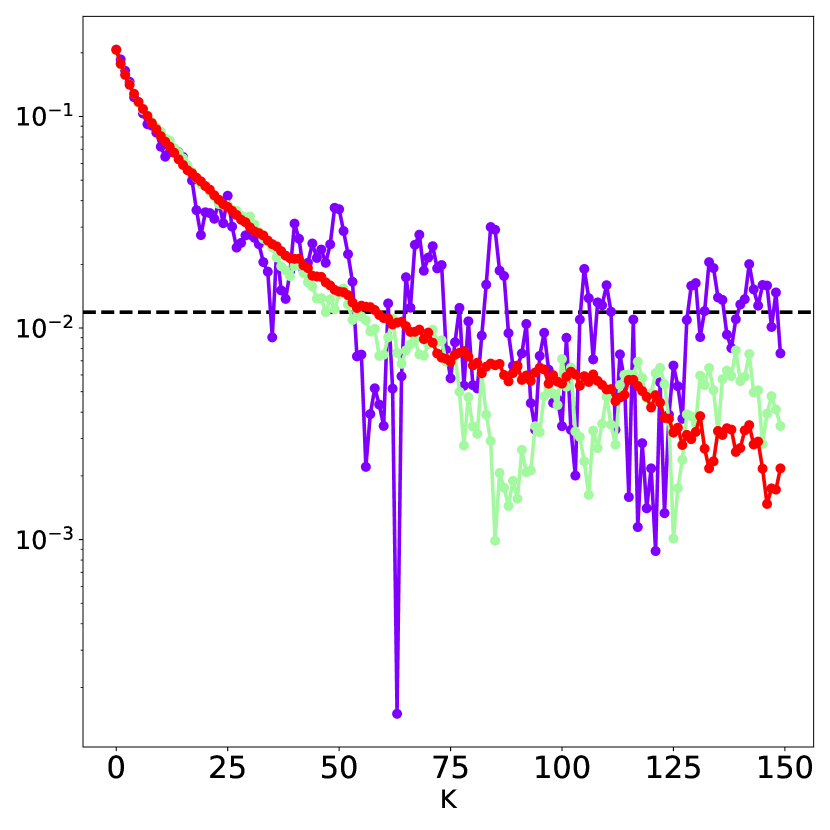
((b)) Bias in log scale

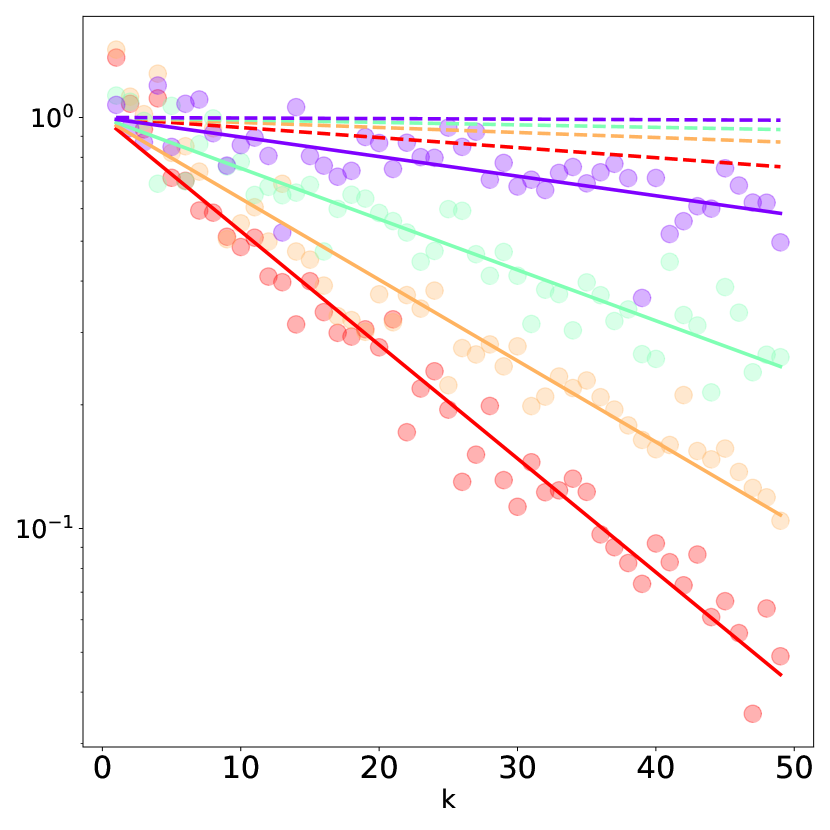
((c)) Sliced Wasserstein

Figure 1:

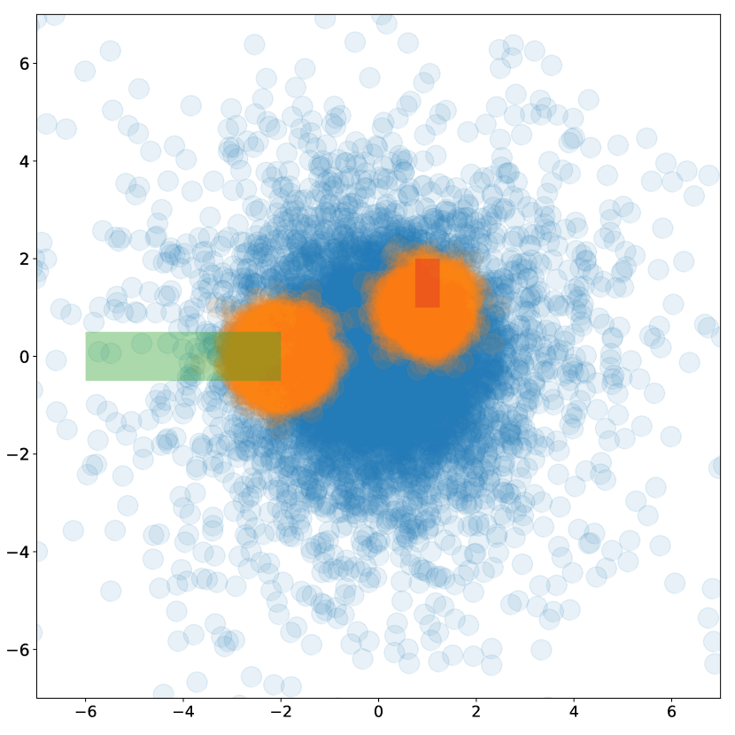
((a)) 2d projection

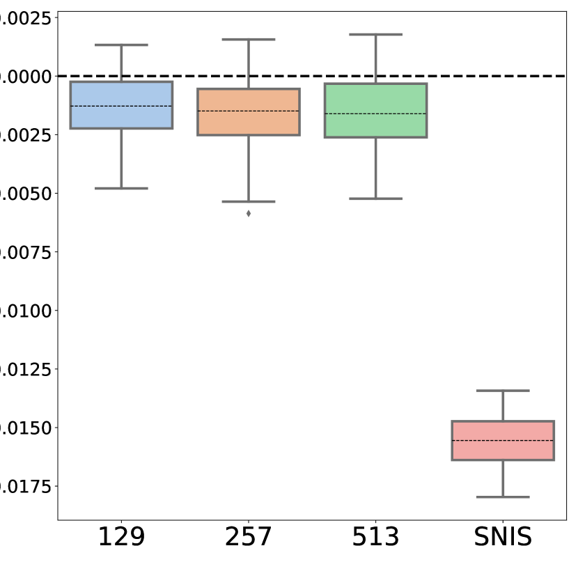
((b)) Bias

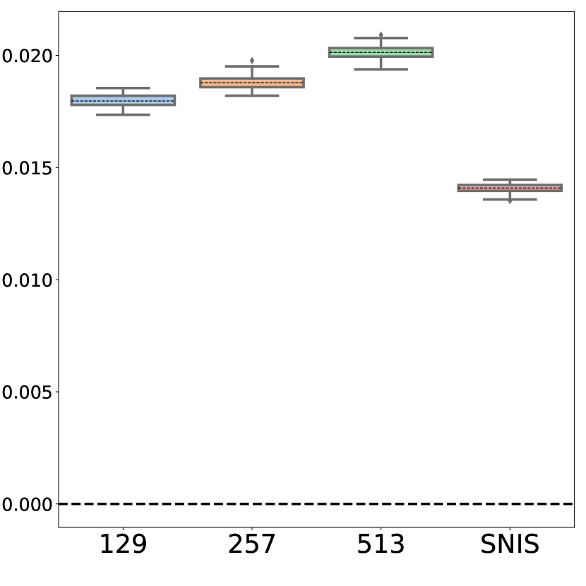
((c)) MSE

Figure 2: Comparison between SNIS and BR-SNIS for the same budget. In each boxplot the dotted line represents the mean value of the samples.

As can be seen from Figure 2(b), BR-SNIS significantly reduces bias (by a factor of almost 10) w.r.t. standard SNIS for both configurations, while MSE increases only slightly (at around $20\%$), as can be seen in Figure 2(c). The code used for this experiment is available at . We also show in Section C.1 that ${k}_{0}=\lfloor 0.625k_{\scriptsize{\mbox{{\it max}}}}\rfloor$ can lead to about $3$ times less bias w.r.t. standard SNIS while only augmenting the MSE of $10\%$. We have also compared in BR-SNIS to zero bias estimators based on SNIS such as [30], the results are in shown in Section C.1.

Bayesian Logistic regression:

We consider posterior inference in a Bayesian logistic regression model. Let $\mathcal{D}_{\scriptsize{\mbox{{\it train}}}}=(\mathbf{x}_{i},y_{i})_{i=1}^{T}$ be a dataset, where each $\mathbf{x}_{i}\in\mathbb{R}^{d}$ is a vector of covariates and $y_{i}\in\{-1,1\}$ is a binary response. Let $p(y_{i}\mid\mathbf{x}_{i};\theta)=\{1+\exp(-y_{i}\,\mathbf{x}_{i}^{\top}\theta)\}^{-1}$ be the probability of the $i$th observation at $\theta\in\Theta\subseteq\mathbb{R}^{d}$ and $\pi_{0}(\mathrm{d}\theta)$ be a prior distribution for $\theta$. The Bayesian posterior is given

$${\textstyle\pi(\mathrm{d}\theta)={\operatorname{Z}}^{-1}\pi_{0}(\mathrm{d}\theta)\exp(\mathcal{L}_{T}(\theta)),\quad\mathcal{L}_{T}(\theta)=\sum_{i=1}^{T}\ln p(y_{i}\mid\mathbf{x}_{i};\theta),\quad\operatorname{Z}=\int\exp(\mathcal{L}_{T}(\theta))\pi_{0}(\mathrm{d}\theta).}$$

For numerical illustration, we use the heart failure clinical records ($d=13$, $T=299$), breast cancer detection ($d=30$, $T=569$), and Covertype ($d=55$, $T=4\cdot 10^{4}$) datasets from the UCI machine learning repository. For Covertype, we use Cover type 1 (Spruce/Fir) and Cover type 2 (Lodgepole Pine) classes to define a binary classification problem. As a prior, we use a Gaussian distribution $\mathrm{N}(0,\tau^{-2}\mathbf{I})$ with $\tau^{2}=5\cdot 10^{-2}$. The importance distribution $\lambda$ is Gaussian with mean and diagonal covariance learned by variational inference; see Section C.2 for details. The boxplots for bias in Figure 3 were constructed in the same way as those in Figure 2.

.	CoverType	Breast	Heart
SNIS, M = 32	0.0028 +/- 0.0012	0.00011 +/- 6.04e-5	0.00023 +/- 7.24e-5
BR-SNIS, M= 32	0.0014 +/- 0.0003	7.9e-5 +/- 5.5e-5	0.00012 +/- 6.7e-5
SNIS, M = 512	0.0026 +/- 0.0017	4.3e-5 +/- 3.3e-5	7.8e-5 +/- 6.8e-5
BR-SNIS, M= 512	0.0013 +/- 0.0003	3.5e-5 +/- 2.2e-5	4.9e-5 +/- 5.2e-5

Table 1: Comparison of the TV distance between the posteriors (Lower is better).

We compare two test functions, $f(\theta)=\theta$, corresponding to evaluation of the posterior mean, and $f(\theta)=p(y\mid\mathbf{x},\theta)$, where $(\mathbf{x},y)\in\mathcal{D}_{\scriptsize{\mbox{{\it test}}}}$. This last function allows us to compute a TV distance for the predictive distribution. Indeed, in a classification context, one can compute the TV distance between any two predictive distributions $p$ and $\hat{p}$ as

$${\textstyle d_{\scriptsize{\mbox{{\it TV}}}}(\hat{p},p)=T^{-1}\sum_{i=1}^{T}\frac{1}{2}\sum_{j=0}^{1}|\hat{p}(y=j\mid\mathbf{x}_{i},\mathcal{D}_{\scriptsize{\mbox{{\it train}}}})-p(y=j\mid\mathbf{x}_{i},\mathcal{D}_{\scriptsize{\mbox{{\it train}}}})|,}$$ (21)

where we compare the predictive distribution $p(y\mid x,\mathcal{D}_{\scriptsize{\mbox{{\it train}}}})=\int p(y\mid x,\theta)\pi(\theta)\mathrm{d}\theta$ and $\hat{p}$ is the estimation of this quantity, provided in the experiments by SNIS or BR-SNIS.

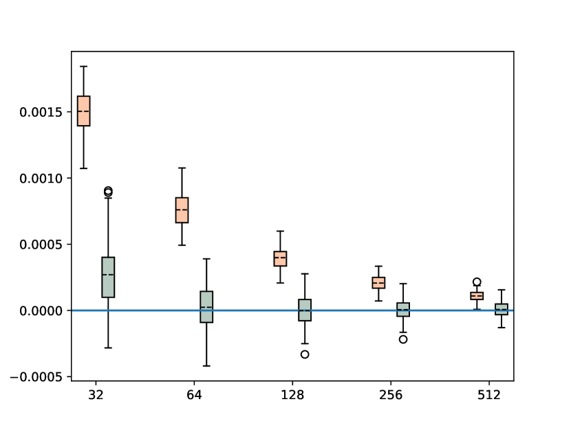
((a)) Heart 8

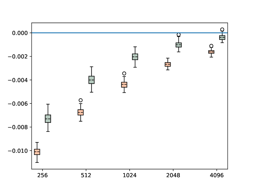
((b)) Breast 11

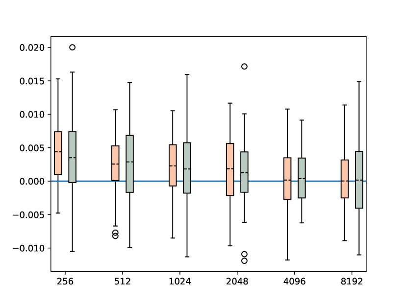
((c)) Covertype 6

Figure 3: Visualization of the distribution for each datasets. Each boxplot is grouped by budget, the left one represent SNIS and the right represent BR-SNIS.

From Figure 3 we can see that for each dataset we have a constant decrease in bias, while the variance increases only slightly. We plot the bias in other components of $\theta$ and provide further numerical details in Section C.2.

Generative Model:

We now extend our methodology to the more complex deep latent generative models (DLGM). A DLGM defines a family of probability densities $p_{\theta}(x)$ over an observation space $x\in\mathbb{R}^{P}$ by introducing a latent variable $z\in\mathbb{R}^{d}$, defining the joint density function $p_{\theta}(x,z)$ (with respect to Lebesgue measure) and aiming to find a parameter $\theta$ maximizing the marginal log-likelihood of the model $p_{\theta}(x)=\int p_{\theta}(x,z)\mathrm{d}z$. Under simple technical assumptions, by Fisher’s identity,

$${\textstyle\nabla_{\theta}\log p_{\theta}(x)=\int\nabla_{\theta}\log p_{\theta}(x,z)p_{\theta}(z\mid x)\mathrm{d}z,}$$ (22)

In most cases, the conditional density $p_{\theta}(z\mid x)=p_{\theta}(x,z)/p_{\theta}(x)$ is intractable and can only be sampled. The variational autoencoder [18] is based on the introduction of an additional parameter $\phi$ and a family of variational distributions $q_{\phi}(z\mid x)$. The joint parameters $\{\theta,\phi\}$ are then inferred by maximizing the evidence lower bound (ELBO) defined by

$$\mathcal{L}(\theta,\phi)=\log p_{\theta}(x)-\mbox{KL}\bigl{(}q_{\phi}(\cdot\mid x)~{}\|~{}p_{\theta}(\cdot\mid x)\bigr{)}\leq\log p_{\theta}(x).$$

This basic setup has been further developed and improved in many directions. Here we consider the importance weighted autoencoder (IWAE) [8], which relies on SNIS to design a tighter ELBO on the log-likelihood. The objective of the IWAE is given by

$${\textstyle\mathcal{L}_{M}(\theta,\phi)=\int\log\left(M^{-1}\sum_{i=1}^{M}w_{\theta,\phi,x}(z_{i})\right)\prod_{\ell=1}^{M}q_{\phi}(z_{\ell}\mid x)\mathrm{d}z_{i},}$$ (23)

where $w_{\theta,\phi,x}(z)={p_{\theta}(x,z)}/{q_{\phi}(z\mid x)}$ denote the importance weights. However, writing, following [8, Eq. (13)],

$${\textstyle\nabla_{\theta}\mathcal{L}_{M}(\theta,\phi)=\int\sum_{i=1}^{M}\omega^{(i)}_{\theta,\phi,x}\nabla_{\theta}\log w_{\theta,\phi,x}(z_{i})\prod_{\ell=1}^{N}q_{\phi}(z_{\ell}\mid x)\mathrm{d}z_{\ell},}$$

where $\omega^{(i)}_{\theta,\phi,x}=w_{\theta,\phi,x}(z_{i})/\sum_{j=1}^{M}w_{\theta,\phi,x}(z_{j})$ are normalized importance weights, yields an expression of the gradient that corresponds exactly to the biased SNIS approximation of (22). Thus, the optimization problem will suffer from bias. We hence propose to use BR-SNIS for learning IWAE. The proposed algorithm proceeds in two steps, which are repeated during the optimization (details are given in Section C.3)

• First, update the parameter $\phi$ as in the IWAE algorithm (using the reparameterization trick and following the methodology of [8]) according to $\phi^{(t+1)}=\phi^{(t)}-\eta\nabla_{\phi}\mathcal{L}_{M}(\theta^{(t)},\phi^{(t)})$.

• Second, update the parameter $\theta$ by estimating (22) using BR-SNIS for $\pi(z)=p_{\theta}(x,z)$, $f(z)=\nabla_{\theta}\log p_{\theta}(x,z)$ and $\lambda(z)=q_{\phi}(z\mid x)$.

d	VAE	IWAE	BR-IWAE ($k=4$)	BR-IWAE ($k=8$)
20	-115.1	-91.5	-90.5	-90.4
50	-96.4	-92.9	-90.1	-90.1

Table 2: Comparison of the mean log likelihood over the MNIST validation set (Higher is better).

We refer to this model as BR-IWAE. As an illustration, we train the model using the binarized MNIST dataset [38], where $x\in\{0,1\}^{784}$ are binarized digits images in dimension 784. For both for the encoder $q_{\phi}$ and the decoder $p_{\theta}$, we use a simple fully connected architecture with 2 hidden layers (more details are given in Section C.3). For a comparison, we estimate the log-likelihood using the VAE, IWAE and BR-IWAE approaches, and the result is reported in Table 2. All models are run for 100 epochs, using the Adam optimizer [17] and a learning rate of $10^{-3}$. The complete experimental details are given in Section C.3.

4 Conclusion

In this paper, we have introduced a novel method, BR-SNIS, which improves over SNIS when it comes to producing close to unbiased estimates of expectations taken w.r.t. to distributions known only up to a normalizing constant, a ubiquitous problem in machine learning and statistics. The high performance of BR-SNIS is supported theoretically by non-asymptotic bias, variance and high-probability bounds. We illustrate our method on various examples, which show the practical advantages of BR-SNIS over SNIS. Finally, BR-SNIS is naturally adapted to other IS based methods, for example [41], which use a Hamiltonian (gradient-based) transform [33] as part of the IS proposal. The extension of BR-SNIS to [41] would produce an Hamiltonian based sampler able to recycle all samples, contrarily to other classical Hamiltonian-based methods [33, 13]. BR-SNIS can also be extended to Particle Markov chain Monte Carlo methods such as Particle Gibbs with Ancestor sampling [26].

Appendix A Proofs

A.1 i-SIR Algorithm

We analyze a slightly modified version of the i-SIR algorithm, with an extra randomization of the state position. The $k$-th iteration is defined as follows. Given a state $Y_{k}\in\mathbbm{X}$,

1. draw $I_{k+1}\in\{1,\dots,N\}$ uniformly at random and set $X^{I_{k+1}}_{k+1}=Y_{k}$;

2. draw $X_{k+1}^{1:N\setminus\{I_{k+1}\}}$ independently from the proposal distribution $\lambda$;

3. compute, for $i\in\{1,\dots,N\}$, the normalized importance weights

   $$\omega^{i}_{N,k+1}=w(X^{i}_{k+1})/\sum_{\ell=1}^{N}w(X^{\ell}_{k+1});$$

4. select $Y_{k+1}$ from the set $X_{k+1}^{1:N}$ by choosing $X_{k+1}^{i}$ with probability $\omega^{i}_{N,k+1}$.

Thus, compared to the simplified i-SIR algorithm given in the introduction, the state is inserted uniformly at random into the list of candidates instead of being inserted at the first position. Of course, this change has no impact as long as we are interested in integrating functions that are permutation invariant with respect to candidates, which is the case throughout our work. Still, this randomization makes the analysis much more transparent.

A.2 Proof of Theorem 1

We write

$$\boldsymbol{\varphi}_{N}(\mathrm{d}(y,x_{1:N})) =\frac{1}{N}\sum_{i=1}^{N}\pi(\mathrm{d}y)\delta_{y}(\mathrm{d}x^{i})\prod_{j\neq i}\lambda(\mathrm{d}x^{j})$$ (24)

$$=\frac{1}{N\lambda(w)}\sum_{i=1}^{N}w(x^{i})\lambda(\mathrm{d}x^{i})\delta_{x^{i}}(\mathrm{d}y)\prod_{j\neq i}\lambda(\mathrm{d}x^{j})$$ (25)

$$=\frac{1}{\lambda(w)}\prod_{j=1}^{N}\lambda(\mathrm{d}x^{j})\Gamma_{N}\mathds{1}_{\mathbbm{X}}(x^{1:N})\sum_{i=1}^{N}\frac{w(x^{i})}{\sum_{\ell=1}^{N}w(x^{\ell})}\delta_{x^{i}}(\mathrm{d}y),$$ (26)

where we recognize, and after having recalled definitions (5) and (6) of $\boldsymbol{\pi}_{N}$ and $\Pi_{N}$, respectively, the right-hand side as $\boldsymbol{\pi}_{N}(\mathrm{d}x^{1:N})\Pi_{N}(x^{1:N},\mathrm{d}y)$. This completes the proof.

A.3 Proof of Theorem 2

Using (6) we get

$$\int\boldsymbol{\pi}_{N}(\mathrm{d}x^{1:N})\Pi_{N}f(x^{1:N}) =\int\frac{1}{N\lambda(w)}\sum_{\ell=1}^{N}w(x^{\ell})\Pi_{N}f(x^{1:N})\prod_{j=1}^{N}\lambda(\mathrm{d}x^{j})$$ (27)

$$=\frac{1}{N\lambda(w)}\int\sum_{i=1}^{N}w(x^{i})f(x^{i})\prod_{j=1}^{N}\lambda(\mathrm{d}x^{j})=\pi(f),$$ (28)

and the proof is complete.

A.4 Proof of Theorem 5

Proof.

We first check that $\boldsymbol{\varphi}_{N}$ is an invariant distribution for $\mathsf{\mathbf{P}}_{N}$. For every $A\in\mathcal{X}^{\varotimes(N+1)}$, using that $\pi$ is the marginal of $\boldsymbol{\varphi}_{N}$ with respect to the state and applying Theorem 1 yields

$$\int\boldsymbol{\varphi}_{N}(\mathrm{d}(y,x^{1:N}))\mathsf{\mathbf{P}}_{N}(y,x^{1:N},A) =\int\pi(\mathrm{d}y)\iint\boldsymbol{\Lambda}_{N}(y,\mathrm{d}\bar{x}^{1:N})\Pi_{N}(\bar{x}^{1:N},\mathrm{d}\bar{y})\mathds{1}_{A}(\bar{y},\bar{x}^{1:N})$$ (29)

$$=\iiint\boldsymbol{\pi}_{N}(\mathrm{d}\bar{x}_{1:N})\Pi_{N}(\bar{x}^{1:N},\mathrm{d}y)\Pi_{N}(\bar{x}^{1:N},\mathrm{d}\bar{y})\mathds{1}_{A}(\bar{y},\bar{x}^{1:N})$$ (30)

$$=\boldsymbol{\varphi}_{N}(A),$$ (31)

which establishes invariance. We now show that $\mathsf{P}_{N}$ is reversible with respect to $\pi$. For this purpose, let $g$ and $h$ be two nonnegative measurable functions and write, using Theorem 1 twice,

$$\iint\pi(\mathrm{d}y)\mathsf{P}_{N}(y,\mathrm{d}\bar{y})g(y)h(\bar{y}) =\int\pi(\mathrm{d}y)\boldsymbol{\Lambda}_{N}(y,\mathrm{d}x^{1:N})\Pi_{N}(x^{1:N},\mathrm{d}\bar{y})g(y)h(\bar{y})$$ (32)

$$=\int\boldsymbol{\pi}_{N}(\mathrm{d}x^{1:N})\Pi_{N}(x^{1:N},\mathrm{d}y)\Pi_{N}(x^{1:N},\mathrm{d}\bar{y})g(y)h(\bar{y})$$ (33)

$$=\int\pi(\mathrm{d}\bar{y})\boldsymbol{\Lambda}_{N}(\bar{y},\mathrm{d}x^{1:N})\Pi_{N}(x^{1:N},\mathrm{d}y)g(y)h(\bar{y})$$ (34)

$$=\iint\pi(\mathrm{d}\bar{y})\mathsf{P}_{N}(\bar{y},\mathrm{d}y)g(y)h(\bar{y}).$$ (35)

∎

A.5 Proof of Theorem 6

For completeness, we repeat the arguments in [25, 5]. Under A 1, we have, for $(x,\mathsf{A})\in\mathbbm{X}\times\mathcal{X}$,

$$\mathsf{P}_{N}(x,\mathsf{A}) =\int\updelta_{x}(\mathrm{d}x^{1})\sum_{i=1}^{N}\frac{w(x^{i})}{\sum_{j=1}^{N}w(x^{j})}\mathds{1}_{\mathsf{A}}(x^{i})\prod_{j=2}^{N}\lambda(\mathrm{d}x^{j})$$ (36)

$$=\int\frac{w(x)}{w(x)+\sum_{j=2}^{N}w(x^{j})}\mathds{1}_{\mathsf{A}}(x)\prod_{j=2}^{N}\lambda(\mathrm{d}x^{j})+\int\sum_{i=2}^{N}\frac{w(x^{i})}{w(x)+\sum_{j=2}^{N}w(x^{j})}\mathds{1}_{\mathsf{A}}(x^{i})\prod_{j=2}^{N}\lambda(\mathrm{d}x^{j})$$ (37)

$$\geq\sum_{i=2}^{N}\int\frac{w(x^{i})}{w(x)+w(x^{i})+\sum_{j=2,j\neq i}^{N}w(x^{j})}\mathds{1}_{\mathsf{A}}(x^{i})\prod_{j=2}^{N}\lambda(\mathrm{d}x^{j})$$ (38)

$$\geq\sum_{i=2}^{N}\int\pi(\mathrm{d}x^{i})\mathds{1}_{\mathsf{A}}(x^{i})\int\frac{\lambda(w)}{w(x)+w(x^{i})+\sum_{j=2,j\neq i}^{N}w(x^{j})}\prod_{j=2,j\neq i}^{N}\lambda(\mathrm{d}x^{j}).$$ (39)

Finally, since the function $f\colon z\mapsto(z+a)^{-1}$ is convex on $\mathbb{R}_{+}$ and $a>0$, we get for $i\in\{2,\dots,N\}$,

$$\int\frac{\lambda(w)}{w(x)+w(x^{i})+\sum_{j=2,j\neq i}^{N}w(x^{j})}\prod_{j=2,j\neq i}^{N}\lambda(\mathrm{d}x^{j})$$ (40)

$$\quad\geq\frac{\lambda(w)}{\int w(x)+w(x^{i})+\sum_{j=2,j\neq i}^{N}w(x^{j})\prod_{j=2,j\neq i}^{N}\lambda(\mathrm{d}x^{j})}$$ (41)

$$\quad\geq\frac{1}{w(x)/\lambda(w)+w(x^{i})/\lambda(w)+N-2}\geq\frac{1}{2\omega+N-2}.$$ (42)

We finally obtain the inequality

$$\mathsf{P}_{N}(x,\mathsf{A})\geq\pi(\mathsf{A})\times\frac{N-1}{2\omega+N-2}=\epsilon_{N}\pi(\mathsf{A}).$$ (43)

This means that the whole space $\mathbbm{X}$ is $(1,\epsilon_{N}\pi)$-small (see [10, Definition 9.3.5]). Since $\mathsf{P}_{N}(x,\cdot)$ and $\pi$ are probability measures, (43) implies

$$\|\mathsf{P}_{N}(x,\cdot)-\pi\|_{\mathrm{TV}}=\sup_{\mathsf{A}\in\mathcal{X}}|\mathsf{P}_{N}(x,\mathsf{A})-\pi(\mathsf{A})|\leq 1-\epsilon_{N}=\kappa_{N}.$$ (44)

Now the statement follows from [10, Theorem 18.2.4] applied with $m=1$.

A.6 Proof of Theorem 3

Proof of ((ii)).

Considering the identity $(a+b)^{2}\leq(1+\epsilon^{2})a^{2}+(1+\epsilon^{-2})b^{2}$, we obtain the decomposition $\{\Pi_{N}f(X_{k}^{1:N})-\pi(f)\}^{2}\leq(1+(N-1)^{-1/2})I+(1+(N-1)^{1/2})II$, with

$$I :=\{\Pi_{N}f(X_{k}^{1:N})-a_{N}(Y_{k-1})/b_{N}(Y_{k-1})\}^{2}$$ (45)

$$II :=\{a_{N}(Y_{k-1})/b_{N}(Y_{k-1})-\pi(f)\}^{2}.$$ (46)

By using the identity $a/b-c/d=(1/d)[(a/b)(d-b)-(c-a)]$, we obtain

$$\Pi_{N}f(X_{k}^{1:N})-a_{N}(Y_{k-1})/b_{N}(Y_{k-1})=b_{N}(Y_{k-1})^{-1}[\Pi_{N}f(X_{k}^{1:N})(b_{N}(Y_{k-1})-\Gamma_{N}\mathds{1}_{\mathbbm{X}}(X_{k}^{1:N}))\\ -(a_{N}(Y_{k-1})-\Gamma_{N}f(X_{k}^{1:N}))].$$ (47)

Therefore, using $(a+b)^{2}\leq 2(a^{2}+b^{2})$ we get

$$I\leq\frac{2}{b_{N}(Y_{k-1})^{2}}[\Pi_{N}f(X_{k}^{1:N})^{2}\{\Gamma_{N}\mathds{1}_{\mathbbm{X}}(X_{k}^{1:N})-b_{N}(Y_{k-1})\}^{2}+\{\Gamma_{N}f(X_{k}^{1:N})-a_{N}(Y_{k-1})\}^{2}].$$ (48)

Using the fact that $\Pi_{N}f(X_{k}^{1:N})^{2}\leq 1$ $\mathbb{P}_{\boldsymbol{\xi}}$-a.s. and $b_{N}(y)\geq(N-1)/N\lambda(w)$, we get, $\mathbb{P}_{\boldsymbol{\xi}}$-a.s.,

$$I\leq\frac{2N^{2}}{(N-1)^{2}\lambda(w)^{2}}\left[\{\Gamma_{N}\mathds{1}_{\mathbbm{X}}(X_{k}^{1:N})-b_{N}(Y_{k-1})\}^{2}+\{\Gamma_{N}f(X_{k}^{1:N})-a_{N}(Y_{k-1})\}^{2}\right]$$ (49)

Therefore, using Lemma (2.2),

$$\mathbb{E}_{{\boldsymbol{\xi}}}[\{\Pi_{N}f(X_{k}^{1:N})-a_{N}(Y_{k-1})/b_{N}(Y_{k-1})\}^{2}]$$ (50)

$$=\mathbb{E}_{{\boldsymbol{\xi}}}[{\mathbb{E}}_{{\boldsymbol{\xi}}}\left[\left.\{\Pi_{N}f(X_{k}^{1:N})-a_{N}(Y_{k-1})/b_{N}(Y_{k-1})\}^{2}\,\right|Y_{k-1}\right]]$$ (51)

$$\leq\frac{2N^{2}}{(N-1)^{2}\lambda(w)^{2}}\left[(N-1)/N^{2}\lambda(\{w-\lambda(w)\}^{2})+(N-1)/N^{2}\lambda(\{wf-\lambda(wf)\}^{2})\right]$$ (52)

$$\leq 4(N-1)^{-1}\kappa[\pi,\lambda].$$ (53)

We consider now $II$. From (20) we have that $II\leq 4N^{-2}(1+\omega)^{2}$, which completes the proof. ∎

Proof of ((iii)).

Note that

$$III :=\mathbb{E}_{{\boldsymbol{\xi}}}[\{\Pi_{N}f(X_{k}^{1:N})-\pi(f)\}\{\Pi_{N}f(X_{k+\ell}^{1:N})-\pi(f)\}]$$ (54)

$$=\mathbb{E}_{{\boldsymbol{\xi}}}[\{\Pi_{N}f(X_{k}^{1:N})-\pi(f)\}{\mathbb{E}}_{{\boldsymbol{\xi}}}\left[\left.\Pi_{N}f(X_{k+\ell}^{1:N})-\pi(f)\,\right|Y_{k+\ell-1}\right]].$$ (55)

As ${\mathbb{E}}_{{\boldsymbol{\xi}}}\left[\left.\Pi_{N}f(X_{k+\ell}^{1:N})\,\right|Y_{k+\ell-1}\right]=\Phi_{N}(Y_{k+\ell-1})$ $\mathbb{P}_{\boldsymbol{\xi}}$-a.s., we have that

$$III =\mathbb{E}_{{\boldsymbol{\xi}}}[\{\Pi_{N}f(X_{k}^{1:N})-\pi(f)\}\{\Phi_{N}(Y_{k+\ell-1})-\pi(f)\}]$$ (56)

$$=\mathbb{E}_{{\boldsymbol{\xi}}}[\{\Pi_{N}f(X_{k}^{1:N})-\pi(f)\}\{{\mathbb{E}}_{{\boldsymbol{\xi}}}\left[\left.\Phi_{N}(Y_{k+\ell-1})\,\right|Y_{k}\right]-\pi(f)\}].$$ (57)

By the Markov property, we get that

$${\mathbb{E}}_{{\boldsymbol{\xi}}}\left[\left.\Phi_{N}(Y_{k+\ell-1})\,\right|Y_{k}\right]=\mathsf{P}_{N}^{\ell-1}\Phi_{N}(Y_{k})=\delta_{Y_{k}}\mathsf{P}_{N}^{\ell-1}\Phi_{N},\quad\mathbb{P}_{\boldsymbol{\xi}}\mbox{-a.s.},$$ (58)

which, combined with (14), implies that

$$\|\mathsf{P}_{N}^{\ell-1}\Phi_{N}-\pi(f)\|_{\infty}\leq\varsigma^{\scriptsize{\mbox{{\it bias}}}}(N-1)^{-1}\kappa_{N}^{\ell-1}.$$ (59)

Combining the results above, we finally establish that

$$|III| \leq\varsigma^{\scriptsize{\mbox{{\it bias}}}}(N-1)^{-1}\kappa_{N}^{\ell-1}\mathbb{E}_{{\boldsymbol{\xi}}}[\{\Pi_{N}f(X_{k}^{1:N})-\pi(f)\}^{2}]^{1/2}$$ (60)

$$\leq\varsigma^{\scriptsize{\mbox{{\it bias}}}}(N-1)^{-1}\kappa_{N}^{\ell-1}\bigl{\{}\sum\nolimits_{i=0}^{2}\varsigma^{\scriptsize{\mbox{{\it mse}}}}_{i}(N-1)^{-1-i/2}\bigr{\}}^{1/2}.$$ (61)

∎

A.7 Proof of Theorem 4

We first consider the bias term. The bound is given by

$$\left|\mathbb{E}_{{\boldsymbol{\xi}}}[\Pi_{(K_{0},K),N}(f)]-\pi(f)\right|\leq(K-K_{0})^{-1}\sum_{\ell=K_{0}+1}^{K}\left|\mathbb{E}_{{\boldsymbol{\xi}}}[\Pi_{N}f(X_{\ell}^{1:N})]-\pi(f)\right|$$ (62)

$$\leq(K-K_{0})^{-1}(N-1)^{-1}\varsigma^{\scriptsize{\mbox{{\it bias}}}}\sum\nolimits_{\ell=K_{0}+1}^{K}\kappa_{N}^{\ell-1}.$$ (63)

The proof is concluded by noting that

$$\sum\nolimits_{\ell=K_{0}+1}^{K}\kappa_{N}^{l-1}\leq\frac{\kappa_{N}^{K_{0}}}{1-\kappa_{N}}\leq\frac{4\tau_{\scriptsize{\mbox{{\it mix}}},N}(1/4)^{K_{0}/\tau_{\scriptsize{\mbox{{\it mix}}},N}}}{3}.$$ (64)

We now consider the MSE, using the decomposition

$$\mathbb{E}_{{\boldsymbol{\xi}}}[(\Pi_{(K_{0},K),N}(f)-\pi(f))^{2}]\leq(K-K_{0})^{-2}\left\{\sum\nolimits_{\ell=K_{0}+1}^{K}\mathbb{E}_{{\boldsymbol{\xi}}}[\Pi_{N}f(X_{\ell}^{1:N})]-\pi(f)\right\}^{2}$$ (65)

$$+2\sum\nolimits_{\ell=K_{0}+1}^{K}\sum\nolimits_{j=\ell+1}^{K}\mathbb{E}_{{\boldsymbol{\xi}}}[\{\Pi_{N}f(X_{\ell}^{1:N})-\pi(f)\}\{\Pi_{N}f(X_{j}^{1:N})-\pi(f)\}].$$ (66)

From the MSE bound of Theorem 9, we have that

$$\sum\nolimits_{\ell=K_{0}+1}^{K}\mathbb{E}_{{\boldsymbol{\xi}}}[\{\Pi_{N}f(X_{\ell}^{1:N})-\pi(f)\}^{2}]\leq(K-K_{0})(N-1)^{-1}\sum\nolimits_{i=0}^{2}\varsigma^{\scriptsize{\mbox{{\it mse}}}}_{i}(N-1)^{-i/2}.$$ (67)

From the covariance bound of Theorem 9, we have that

$$\sum_{\ell=K_{0}+1}^{K}\sum_{j=\ell+1}^{K}\mathbb{E}_{{\boldsymbol{\xi}}}[\{\Pi_{N}f(X_{\ell}^{1:N})-\pi(f)\}\{\Pi_{N}f(X_{j}^{1:N})-\pi(f)\}]\\ \leq\sum_{i=0}^{2}\varsigma^{\scriptsize{\mbox{{\it cov}}}}_{i}(N-1)^{-\frac{3-i/2}{2}}\left[\sum_{\ell=K_{0}+1}^{K}\sum_{j=\ell+1}^{K}\kappa_{N}^{(j-\ell)-1}\right].$$ (68)

As $\sum\nolimits_{\ell=K_{0}+1}^{K}\sum\nolimits_{j=\ell+1}^{K}\kappa_{N}^{(j-\ell)-1}\leq(K-K_{0})(4/3)\tau_{\scriptsize{\mbox{{\it mix}}},N}$ we have

$$\mathbb{E}_{{\boldsymbol{\xi}}}[(\Pi_{(K_{0},K),N}(f)-\pi(f))^{2}]\leq((K-K_{0})(N-1))^{-1}\left[\sum\nolimits_{i=0}^{2}\varsigma^{\scriptsize{\mbox{{\it mse}}}}_{i}(N-1)^{-i/2}\right]$$ (69)

$$+(8/3)(K-K_{0})^{-1}(N-1)^{-3/2}\left[\sum_{i=0}^{2}\varsigma^{\scriptsize{\mbox{{\it cov}}}}_{i}(N-1)^{-i/4}\right].$$ (70)

The proof for the MSE is concluded by noting that $(K-K_{0})(N-1)=\upsilon M$ and noting that $\mathsf{MSE}^{\scriptsize{\mbox{{\it is}}}}_{M}:=\varsigma^{\scriptsize{\mbox{{\it mse}}}}_{0}M^{-1}$.

The high-probability bound requires more complex derivations. We use the decomposition

$$\Pi_{(K_{0},K),N}(f)-\pi(f)=(K-K_{0})^{-1}\sum_{k=K_{0}+1}^{K}\Pi_{N}f(X_{k}^{1:N})-\Phi_{N}(Y_{k-1})\\ +(K-K_{0})^{-1}\sum_{k=K_{0}+1}^{K-1}\Phi_{N}(Y_{k-1})-\pi(\Phi_{N}).$$ (71)

where we have used $\pi(f)=\pi(\Phi_{N})$. Therefore, for any $t\geq 0$, we get that

$$\mathbb{P}_{{\boldsymbol{\xi}}}(|\Pi_{(K_{0},K),N}(f)-\pi(f)|\geq t)\leq\mathbb{P}_{{\boldsymbol{\xi}}}\left((K-K_{0})^{-1}\left|\sum\nolimits_{k=K_{0}+1}^{K}\Pi_{N}f(X_{k}^{1:N})-\Phi_{N}(Y_{k-1})\right|\geq t/2\right)\\ +\mathbb{P}_{{\boldsymbol{\xi}}}\left((K-K_{0})^{-1}\left|\sum\nolimits_{k=K_{0}+1}^{K-1}\Phi_{N}(Y_{k-1})-\pi(\Phi_{N})\right|\geq t/2\right).$$ (72)

We will show that for all $t>0$, and for some absolute constants $\zeta_{I}$, $\zeta_{II}$,

$$I:=\mathbb{P}_{{\boldsymbol{\xi}}}\left((K-K_{0})^{-1}\left|\sum\nolimits_{k=K_{0}+1}^{K}\Pi_{N}f(X_{k}^{1:N})-\Phi_{N}(Y_{k-1})\right|\geq t\right)\leq 2\exp(-t^{2}\upsilon M/(4\zeta_{I})),$$ (73)

$$II:=\mathbb{P}_{{\boldsymbol{\xi}}}\left((K-K_{0})^{-1}\left|\sum\nolimits_{k=K_{0}+1}^{K-1}\Phi_{N}(Y_{k-1})-\pi(\Phi_{N})\right|\geq t\right)\leq 2\exp(-t^{2}\zeta_{II}(K-K_{0})(N-1)^{2}/\tau_{\scriptsize{\mbox{{\it mix}}},N}).$$ (74)

Consider first $I$. Note first that

$$I=\mathbb{E}_{{\boldsymbol{\xi}}}\left[{\mathbb{P}}_{{\boldsymbol{\xi}}}\left[\left.(K-K_{0})^{-1}\left|\sum\nolimits_{k=K_{0}+1}^{K}\Pi_{N}f(X_{k}^{1:N})-\Phi_{N}(Y_{k-1})\right|\geq t\,\right|Y_{K_{0}:K-1}\right]\right].$$ (75)

By Theorem 5, the random elements $\{X_{k}^{1:N}\}_{k=K_{0}+1}^{K}$ are independent conditionally to $\{Y_{k}\}_{k=K_{0}}^{K-1}$. Using the generalized Hoeffding inequality (see [44, Theorem 2.6.2] or [45, Proposition 2.1]), we get, with $\Delta_{N,k}:=\Pi_{N}f(X_{k}^{1:N})-\Phi_{N}(Y_{k-1})$, that

$${\mathbb{P}}_{{\boldsymbol{\xi}}}\left[\left.(K-K_{0})^{-1}\left|\sum\nolimits_{k=K_{0}+1}^{K}\Delta_{N,k}\right|\geq t\,\right|Y_{K_{0}:K-1}\right]\leq 2\exp\left(-\frac{t^{2}(K-K_{0})^{2}}{4\sum_{k=K_{0}+1}^{K}\|\Delta_{N,k}\|_{\psi_{2},Y_{k}}^{2}}\right),$$ (76)

where $\psi_{2}(x)=\exp(x^{2})-1$ and

$$\|\Delta_{N,k}\|_{\psi_{2},Y_{k-1}}=\inf\left\{\lambda>0~{}:~{}{\mathbb{E}}_{{\boldsymbol{\xi}}}\left[\left.\psi_{2}(|\Delta_{N,k}|/\lambda)\,\right|Y_{k-1}\right]\leq 1\right\}.$$

We have to bound $\|\Delta_{N,k}\|_{\psi_{2},Y_{k-1}}$. We use the decomposition

$$\Delta_{N,k}=\left\{\frac{\Gamma_{N}f(X_{k}^{1:N})}{\Gamma_{N}\mathds{1}_{\mathbbm{X}}(X_{k}^{1:N})}-\frac{a_{N}(Y_{k-1})}{b_{N}(Y_{k-1})}\right\}+\left\{\frac{a_{N}(Y_{k-1})}{b_{N}(Y_{k-1})}-\Phi_{N}(Y_{k-1})\right\}=:\Delta_{N,k}^{I}+\Delta_{N,k}^{II}.$$ (77)

combined with Appendix B with $\phi=\psi_{2}$ and $\chi=\psi_{2}$ and [44, Proposition 2.6.1]. By (18) and by [44, Equation 2.17] we have that

$$\|\Delta_{N,k}^{II}\|_{\psi_{2},Y_{k-1}}\leq 2\log(2)^{-1/2}(N-1)^{-1}\kappa[\lambda,\pi].$$ (78)

Using Appendix B with $\phi=\chi=\psi_{2}$ and the fact that $b_{N}(y)\geq(1-1/N)\lambda(w)$ we have that

$$\|\Delta_{N,k}^{I}\|_{\psi_{2},Y_{k-1}}\leq\frac{2}{(1-1/N)\lambda(w)}\\ \times\left[\|\Gamma_{N}f(X_{k}^{1:N})-a_{N}(Y_{k-1})\|_{\psi_{2},Y_{k-1}}+2\|\Gamma_{N}\mathds{1}_{\mathbbm{X}}(X_{k}^{1:N})-b_{N}(Y_{k-1})\|_{\psi_{2},Y_{k-1}}\right].$$ (79)

Using [44, Proposition 2.6.1, Eq 2.17], we get that, $\mathbb{P}_{{\boldsymbol{\xi}}}$-a.s.,

$$\|\Gamma_{N}f(X_{k-1}^{1:N})-a_{N}(Y_{k-1})\|^{2}_{\psi_{2},Y_{k-1}} \leq 64\mathrm{e}/\log{2}N^{-1}\|w(X_{k}^{1})f(X_{k}^{1})-{\mathbb{E}}_{{\boldsymbol{\xi}}}\left[\left.w(X_{k}^{1})f(X_{k}^{1})\,\right|Y_{k-1}\right]\|^{2}_{\psi_{2},Y_{k-1}},$$ (80)

$$\leq 256\mathrm{e}/\log{(2)}^{2}N^{-1}\|w\|_{\infty}^{2}.$$ (81)

The same bound applies to $\|\Gamma_{N}\mathds{1}_{\mathbbm{X}}(X_{k}^{1:N})-b_{N}(Y_{k-1})\|^{2}_{\psi_{2},Y_{k-1}}$ and we can write

$$\|\Delta_{N,k}^{I}\|_{\psi_{2},Y_{k-1}}\leq 96e^{1/2}\log(2)^{-1}(N-1)^{-1/2}\omega.$$ (82)

We can now conclude by writing

$$\|\Delta_{N,k}\|_{\psi_{2},Y_{k-1}}^{2} \leq 2(\|\Delta_{N,k}^{I}\|_{\psi_{2},Y_{k-1}}^{2}+\|\Delta_{N,k}^{II}\|_{\psi_{2},Y_{k-1}}^{2})$$ (83)

$$\leq(N-1)^{-1}(\zeta_{I,1}\omega^{2}+\zeta_{I,2}\kappa[\lambda,\pi]^{2}(N-1)^{-1}),$$ (84)

where $\zeta_{I,1}=18432\mathrm{e}\log(2)^{-2}$ and $\zeta_{I,2}=8\log(2)^{-1}$ are absolute constants, which imply

$$\|\Delta_{N,k}\|_{\psi_{2},Y_{k-1}}^{2}\leq\zeta_{I}(N-1)^{-1},$$ (85)

with $\zeta_{I}=1.1\cdot 10^{5}\omega^{2}$. This finally concludes $I\leq 2\exp(-t^{2}\upsilon M/4\zeta_{I})$.

Consider now $II$. We use Appendix B with $g_{i}=\Phi_{N}(Y_{K_{0}+i-1})-\pi(\Phi_{N})$. As $\|g_{i}\|_{\infty}\leq\operatorname{osc}(\Phi_{N})\leq(N-1)^{-1}\varsigma^{\scriptsize{\mbox{{\it bias}}}}$, we obtain

$$II\leq 2\exp\left(-t^{2}\zeta_{II}(K-K_{0})(N-1)^{2}/\tau_{\scriptsize{\mbox{{\it mix}}},N}\right)$$ (86)

where $\zeta_{II}=\frac{2}{(3\varsigma^{\scriptsize{\mbox{{\it bias}}}})^{2}}$. Finally, we obtain

$$\mathbb{P}_{{\boldsymbol{\xi}}}(|\Pi_{(K_{0},K),N}(f)-\pi(f)|\geq t)\leq 2\exp(-t^{2}\upsilon M/4\zeta_{I})[1+\exp(-t^{2}\upsilon M\{\zeta_{II}(N-1)/\tau_{\scriptsize{\mbox{{\it mix}}},N}-(4\zeta_{I})^{-1}\})].$$ (87)

We conclude by noting that, for any $\delta\in(0,1)$, if $(N-1)\geq\tau_{\scriptsize{\mbox{{\it mix}}},N}(4\zeta_{I}\zeta_{II})^{-1}$, we have that

$$\mathbb{P}_{{\boldsymbol{\xi}}}(|\Pi_{(K_{0},K),N}(f)-\pi(f)|\geq t)\leq 4\exp(-t^{2}\upsilon M/4\zeta_{I})\leq\delta$$ (88)

for all $t\geq 2\zeta_{I}^{1/2}(\upsilon M)^{-1/2}\log(4/\delta)^{1/2}$. This concludes the proof with $\varsigma^{\scriptsize{\mbox{{\it hpd}}}}=2\zeta_{I}^{1/2}$.

A.8 High probability inequality for SNIS

Theorem 7.

Assume that $\omega=\|w\|_{\infty}/\lambda(w)<\infty$. For any bounded measurable function $f$ on $(\mathbbm{X},\mathcal{X})$ such that $\|f\|_{\infty}\leq 1$, for any $M>1$ and for any $\delta$ in $(0,1)$,

$$|\widehat{\pi}_{M}(f)-\pi(f)|\leq 12\omega[M\log(2)]^{-1/2}\log(2/\delta)^{1/2}$$ (89)

with probability larger than $1-\delta$.

Proof.

Let $A_{M}=M^{-1}\sum\nolimits_{i=1}^{M}w(X^{i})f(X^{i})$, $B_{M}=M^{-1}\sum\nolimits_{i=1}^{M}w(X^{i})$, $a=\mathbb{E}(A_{M})=\lambda(wf)$ and $b=\mathbb{E}(B_{M})=\lambda(w)$. Note that $\widehat{\pi}_{M}(f)=A_{M}/B_{M}$ and $\pi(f)=a/b$. By Appendix B with $\phi=\chi=\exp(x^{2})-1$, we have that:

$$\|\widehat{\pi}_{M}(f)-\pi(f)\|_{\psi_{2}}\leq 2\lambda(w)^{-1}[\|A_{M}-a\|_{\psi_{2}}+2\|B_{M}-b\|_{\psi_{2}}].$$ (90)

Using [44, Eq 2.17], we get that, $\mathbb{P}_{{\boldsymbol{\xi}}}$-a.s.

$$\|A_{M}-a\|_{\psi_{2}}^{2}\leq M^{-1}\|w(X^{i})f(X^{i})-\lambda(wf)\|_{\psi_{2}}^{2}\leq 4(\log(2)M)^{-1}\|w\|_{\infty}^{2}.$$ (91)

In the same way, $\|B_{M}-b\|_{\psi_{2}}^{2}\leq 4(\log(2)M)^{-1}\|w\|_{\infty}^{2}$. Therefore, we have that:

$$\|\widehat{\pi}_{M}(f)-\pi(f)\|_{\psi_{2}}^{2}\leq(12\omega)^{2}(\log(2)M)^{-1}.$$ (92)

Combining it with [44, Proposition 2.5.2], we have that:

$$\mathbb{P}(|\widehat{\pi}_{M}(f)-\pi(f)|\geq t)\leq 2\exp(-t^{2}\zeta^{\operatorname{snis}}M)$$ (93)

where $\zeta^{\operatorname{snis}}=\log(2)(12\omega)^{-2}$. The high probability inequality follows directly. ∎

Appendix B Moments and high-probability bounds for ratio statistics

Let $(U_{i},V_{i})_{i\in\{1,\dots,n\}}$ be (possibly dependent) random variables defined on some probability space $(\Omega,\mathcal{F},\mathbb{P})$. Assume that $U_{i}\geq 0$, $\mathbb{P}$-a.s.. Moreover, let $\hat{A}_{n}=n^{-1}\sum_{i=1}^{n}U_{i}V_{i}$, $\hat{B}_{n}=n^{-1}\sum_{i=1}^{n}U_{i}$, $\hat{R}_{n}=\hat{A}_{n}/\hat{B}_{n}$ and $a=\mathbb{E}\left[\hat{A}_{n}\right]$, $b=\mathbb{E}\left[\hat{B}_{n}\right]$, and $r=a/b$.

A continuous, even, convex function $\phi:\mathbb{R}^{+}\to\left[0,+\infty\right]$ is a Young function if $\phi$ is monotonically increasing for $x>0$, $\phi(0)=0$, $\lim_{x\to\infty}\phi(x)/x=\infty$, and $\lim_{x\to 0^{+}}\phi(x)/x=0$. We denote by $\phi^{*}$ the Fenchel-Legendre conjugate of $\phi$. Let $X$ be a random variable and $\phi$ be a Young function. Then the Orlicz norm of $X$ is

$$\|X\|_{\phi}=\inf\left\{\lambda>0~{}:~{}\mathbb{E}\left[\phi\left(|X|/\lambda\right)\right]\leq 1\right\}\,,$$ (94)

with the convention that $\inf\emptyset=\infty$. The Orlicz space of random variable $\mathcal{L}_{\phi}(\Omega)$ is the family of equivalence classes of random variables $X$ such that $\|X\|_{\phi}<\infty$. $\mathcal{L}_{\phi}(\Omega)$ is a Banach space. If $\phi_{p}(x)=|x|^{p}$ for $p\geq 1$, then $\mathcal{L}_{\phi}(\Omega)=\mathcal{L}^{p}(\Omega)$ and we denote $\|\cdot\|_{p}=\|\cdot\|_{\phi_{p}}$. If $X\in\mathcal{L}_{\phi}(\Omega)$, then, for any $x>0$

$$\mathbb{P}(|X|\geq x)\leq 1/\phi(x/\|X\|_{\phi}),\quad\text{and}\quad\|\mathds{1}_{\{|X|\geq x\}}\|_{\phi}=1/\phi^{-1}(1/\mathbb{P}(|X|\geq x)).$$

Lemma .

Let $\phi,\chi$ be Young functions. If $\max_{i}\|V_{i}\|_{\infty}\leq c|r|$, then

$$\|\hat{R}_{n}-r\|_{\phi}/|r|\leq 2\|\hat{A}_{n}-a\|_{\phi}/b+2\|\hat{B}_{n}-b\|_{\phi}/b+c/\{(\phi^{-1}\circ\chi)(b/2\|(\hat{B}_{n}-b)_{-}\|_{\chi})\}\,.$$ (95)

Proof.

We decompose the computation in two parts: first, when $\hat{B}_{n}>b/2$, we have

$$|\hat{R}_{n}-r| =\left|\frac{\hat{A}_{n}-a}{\hat{B}_{n}}+a\left(\frac{1}{\hat{B}_{n}}-\frac{1}{b}\right)\right|\leq\frac{|\hat{A}_{n}-a|}{\hat{B}_{n}}+\frac{|a||\hat{B}_{n}-b|}{\hat{B}_{n}b}$$ (96)

$$\leq\frac{|\hat{A}_{n}-a|}{b/2}+\frac{|a||\hat{B}_{n}-b|}{(b/2)b}=\frac{2|\hat{A}_{n}-a|}{b}+\frac{2|r||\hat{B}_{n}-b|}{b}\,.$$ (97)

Then, when $\hat{B}_{n}\leq b/2$, we have

$$|\hat{R}_{n}-r| \leq|\hat{R}_{n}|+|r|\leq|\hat{R}_{n}|+\frac{2|r||\hat{B}_{n}-b|}{b}\leq\max_{i}|V_{i}|+\frac{2|r||\hat{B}_{n}-b|}{b}\,,$$ (98)

where the second inequality follows from $|\hat{B}_{n}-b|\geq b/2$. Combining the two previous inequalities, we have

$$|\hat{R}_{n}-r|\leq\frac{2|\hat{A}_{n}-a|}{b}+\frac{2|r||\hat{B}_{n}-b|}{b}+\max_{i}|V_{i}|\mathds{1}_{\{\hat{B}_{n}\leq b/2\}}\,.$$ (99)

Recall that, if $|X|\leq|Y|$ a.s., then $\|X\|_{\phi}\leq\|Y\|_{\phi}$. Hence, we get that

$$\|\hat{R}_{n}-r\|_{\phi} \leq\left\|\frac{2|\hat{A}_{n}-a|}{b}+\frac{2r|\hat{B}_{n}-b|}{b}+\max_{i}|V_{i}|\mathds{1}_{\{\hat{B}_{n}\leq b/2\}}\right\|_{\phi}$$ (100)

$$\leq\left\|\frac{2\hat{A}_{n}-a}{b}\right\|_{\phi}+\left\|\frac{2|r||\hat{B}_{n}-b|}{b}\right\|_{\phi}+\left\|\max_{i}|V_{i}|\mathds{1}_{\{\hat{B}_{n}\leq b/2\}}\right\|_{\phi}$$ (101)

$$=\frac{2\|\hat{A}_{n}-a\|_{\phi}}{b}+\frac{2|r|\|\hat{B}_{n}-b\|_{\phi}}{b}+\|\max_{i}|V_{i}|\mathds{1}_{\{\hat{B}_{n}\leq b/2\}}\|_{\phi}$$ (102)

$$\leq\frac{2\|\hat{A}_{n}-a\|_{\phi}}{b}+\frac{2|r|\|\hat{B}_{n}-b\|_{\phi}}{b}+c|r|\|\mathds{1}_{\{\hat{B}_{n}\leq b/2\}}\|_{\phi}$$ (103)

$$=\frac{2\|\hat{A}_{n}-a\|_{\phi}}{b}+\frac{2|r|\|\hat{B}_{n}-b\|_{\phi}}{b}+c|r|/\phi^{-1}\left(1/\mathbb{P}(\hat{B}_{n}\leq b/2)\right)\,.$$ (104)

Finally, we obtain the desired result by noting that, for any Young function $\chi$, $\mathbb{P}(\hat{B}_{n}\leq b/2)=\mathbb{P}(|(\hat{B}_{n}-b)_{-}|\geq b/2)\leq 1/{\chi(b/2\|(\hat{B}_{n}-b)_{-}\|_{\chi})}$. ∎

Theorem 8.

Let $p\geq 1$. If $\max_{i}\|V_{i}\|_{\infty}\leq c|r|$, then

$$\frac{\|\hat{R}_{n}-r\|_{p}}{|r|}\leq\frac{2\|\hat{A}_{n}-a\|_{p}}{b}+\frac{2(1+c)\|\hat{B}_{n}-b\|_{p}}{b}\,.$$ (105)

Proof.

Apply Appendix B with $\chi(x)=\phi(x)=x^{p}$. ∎

Theorem 9 (Bias of the estimator).

If $|\hat{A}_{n}/\hat{B}_{n}|\leq 1$, then

$$\left|\mathbb{E}[\hat{R}_{n}]-r\right|\leq(2b^{2})^{-1}\{3\mathbb{E}[\{\hat{B}_{n}-b\}^{2}]+\mathbb{E}[\{\hat{A}_{n}-a\}^{2}]\}.$$ (106)

Proof.

We use the elementary identity

$$\frac{\hat{A}_{n}}{\hat{B}_{n}}-\frac{a}{b}=\frac{\hat{A}_{n}}{\hat{B}_{n}}\frac{(b-\hat{B}_{n})^{2}}{b^{2}}+\frac{(\hat{A}_{n}-a)(b-\hat{B}_{n})}{b^{2}}+\frac{a(b-\hat{B}_{n})}{b^{2}}+\frac{\hat{A}_{n}-a}{b},$$ (107)

which implies that

$$\mathbb{E}[\hat{R}_{n}]-r=\mathbb{E}\left[\frac{\hat{A}_{n}}{\hat{B}_{n}}\frac{(b-\hat{B}_{n})^{2}}{b^{2}}\right]+\frac{\mathbb{E}[(\hat{A}_{n}-a)(b-\hat{B}_{n})]}{b^{2}}$$

∎

We conclude with a lemma that gives the concentration of a uniformly ergodic Markov chain. We think that this Lemma is of independent interest, and we give it under general conditions.

Lemma .

Let $(\mathbbm{Z},\mathcal{Z})$ be a state-space and $\operatorname{Q}$ a Markov kernel on $(\mathbbm{Z},\mathcal{Z})$ which is uniformly ergodic with mixing time $t_{\operatorname{mix}}$ and stationary distribution $\pi$. Let $\{g_{i}\}_{i=1}^{n}$ be a family of measurable functions from $\mathbbm{Z}$ to $\mathbb{R}^{d}$ such that $\|g\|_{\infty}=\max_{i\in\{1,\ldots,n\}}\|g_{i}\|_{\infty}<\infty$ and $\pi(g_{i})=0$ for any $i\in\{1,\ldots,n\}$. Then, for any initial probability $\xi$ on $(\mathbbm{Z},\mathcal{Z})$, $n\in\mathbb{N}$, $t\geq 0$, it holds

$$\mathbb{P}_{\xi}\biggl{(}\|{\sum\nolimits_{i=1}^{n}g_{i}(Z_{i})}\|\geq t\biggr{)}\leq 2\exp\biggl{\{}-\frac{2t^{2}}{u_{n}^{2}}\biggr{\}},\text{ where }u_{n}=3\|g\|_{\infty}\sqrt{n}\sqrt{t_{\operatorname{mix}}}.$$ (108)

Proof.

The function $\varphi(x^{1:N}_{1},\dots,x^{1:N}_{n}):=\|\sum_{i=1}^{n}g_{i}(x^{1:N}_{i})\|$ on $\mathbbm{Z}^{n}$ satisfies the bounded differences property. Applying [35, Corollary 2.10], we get for $t\geq\mathbb{E}_{\xi}[\|\sum_{i=1}^{n}g_{i}(Z_{i})\|]$,

$$\mathbb{P}_{\xi}\biggl{(}\|\sum\nolimits_{i=1}^{n}g_{i}(Z_{i})\|\geq t\biggr{)}\leq\exp\left\{-\frac{2(t-\mathbb{E}_{\xi}[\|\sum_{i=1}^{n}g_{i}(Z_{i})\|])^{2}}{9n\|g\|_{\infty}^{2}t_{\operatorname{mix}}}\right\}.$$ (109)

It remains to upper bound $\mathbb{E}_{\xi}[\|\sum_{i=1}^{n}g_{i}(Z_{i})\|]$. Note that

$$\mathbb{E}_{\xi}[\|\sum\nolimits_{i=1}^{n}g_{i}(Z_{i})\|^{2}]=\sum\nolimits_{i=1}^{n}\mathbb{E}_{\xi}[\|g_{i}(Z_{i})\|^{2}]+2\sum\nolimits_{k=1}^{n-1}\sum\nolimits_{\ell=1}^{n-k}\mathbb{E}_{\xi}[g_{k}(Z_{k})^{\top}g_{k+\ell}(Z_{k+\ell})]$$ (110)

and, using $\pi(g_{k+\ell})=0$, we obtain

$$\textstyle\bigl{|}\mathbb{E}_{\xi}[g_{k}(Z_{k})^{\top}g_{k+\ell}(Z_{k+\ell})]\bigr{|} =\left|\int_{\mathbbm{Z}}g_{k}(z)^{\top}\left(\operatorname{Q}^{\ell}g_{k+\ell}(z)-\pi(g_{k+\ell})\right)\xi\operatorname{Q}^{k}(\mathrm{d}z)\right|\leq\|g\|_{\infty}^{2}(1/4)^{\lceil\ell/t_{\operatorname{mix}}\rceil}.$$ (111)

which implies

$$\textstyle\sum_{k=1}^{n-1}\sum_{\ell=1}^{n-k}|\mathbb{E}_{\xi}[g_{k}(Z_{k})^{\top}g_{k+\ell}(Z_{k+\ell})]| \leq\sum_{k=1}^{n-1}\|g\|_{\infty}^{2}(1/4)^{\lceil\ell/t_{\operatorname{mix}}\rceil}\leq(4/3)\|g\|_{\infty}^{2}t_{\operatorname{mix}}n.$$ (112)

Combining the bounds above, we upper bound $\mathbb{E}_{\xi}[\|\sum_{i=1}^{n}g_{i}(Z_{i})\|]$ as

$$\mathbb{E}_{\xi}[\|\sum\nolimits_{i=1}^{n}g_{i}(Z_{i})\|] \leq\bigl{\{}\mathbb{E}_{\xi}[\|\sum\nolimits_{i=1}^{n}g_{i}(Z_{i})\|^{2}]\bigr{\}}^{1/2}\leq 2\sqrt{n}\|g\|_{\infty}\sqrt{t_{\operatorname{mix}}}=:v_{n}.$$ (113)

Plugging this result in (108), we obtain that

$$\mathbb{P}_{\xi}\biggl{(}\|\sum\nolimits_{i=1}^{n}g_{i}(Z_{i})\|\geq t\biggr{)}\leq\begin{cases}1,\quad t<v_{n},\\ \exp\left\{-\frac{2(t-v_{n})^{2}}{9v_{n}^{2}}\right\},\quad t\geq v_{n}.\end{cases}$$ (114)

Now it is easy to see that right-hand side of (114) is upper bounded by $2\exp\{-2t^{2}/(9v_{n}^{2})\}$ for any $t\geq 0$, and the statement follows. ∎

Appendix C Experiments

C.1 Gaussian Mixture

Bias MSE trade-off:

We display in Figures 4(a) and 4(b) the bias and the MSE of the BR-SNIS estimators for the same configuration as in Figure 2 but with ${k}_{0}=\lfloor 0.625k_{\scriptsize{\mbox{{\it max}}}}\rfloor$. We observe $3$ times less bias than the SNIS estimators but only with a $10\%$ increase of the MSE for the $N=129$ setting. This can be also seen in Figure 4(c), where we show the ratio between BR-SNIS and SNIS for bias and MSE with $N=129$.

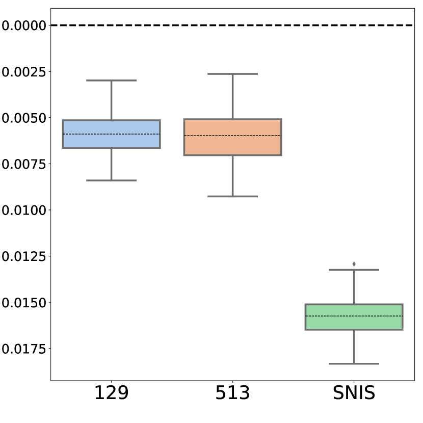
((a)) Bias

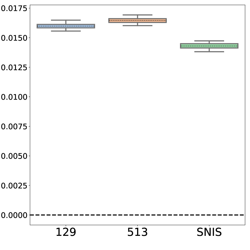
((b)) MSE

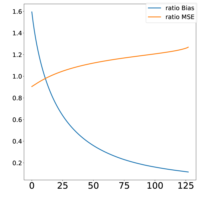
((c)) Ratios as ${k}_{0}$

Figure 4: Comparison between SNIS and BR-SNIS for the same budget. In each boxplot the dotted line represents the mean value of the samples. In Figure 4(c) we display the ratio between BR-SNIS and SNIS for bias and MSE with $N=129$.

Parameters Gaussian mixture:

The $\pi$ in Section 3 is a Mixture of two Gaussians in dimension $7$ with mean vectors $\boldsymbol{\mu}_{1}=(1,\dots,1)^{\intercal}$ and $\boldsymbol{\mu}_{2}=(-2,0,\dots,0)^{\intercal}$ and covariance matrices $\boldsymbol{\Sigma}_{1}=d^{-1}\mathbf{I}$ and $\boldsymbol{\Sigma}_{2}=d^{-1}\mathbf{I}$, where $p=1/3$ and $\mathbf{I}$ is the identity matrix In this setting, the quantities $\kappa[\pi,\lambda]$ and $\omega$ can be estimated by Monte Carlo and Gradient ascent respectively. Their values are approximately $7\cdot 10^{2}$ and $1\cdot 10^{4}$, respectively.

The sets $A$ and $B$ used to define the function $f$ are the following:

$$A:=[-2,6]\times[-1,1]^{6},\quad B:=[0.75,1.25]\times[1,2]\times[-0.1,0.1]^{5}.$$ (115)

We used this example to illustrate numerically the bounds in Theorems 3 and 4, where each expectation was calculated by Monte Carlo using $2\cdot 10^{4}$ samples. We displayed in each figure the equivalent SNIS estimation in a green dashed line. For all the bias related bounds(Theorem 3(i) in Figure 5(a), Theorem 4(i) in Figure 5(c)), we fixed a total budget of $M=6\cdot 10^{3}$. For Figure 5(a) we added a fit of the type $y=\exp(ak+b)$ to illustrate the exponential decay w.r.t. $k$.

We then increased the budget to $M=8\cdot 10^{4}$ for the MSE and covariance bounds, in order to fully observe the stabilisation of the MSE in Figure 5(b) for all the minibatch sizes $N$. For the true value of $\pi(f)$ needed for calculating the MSE, we use an estimation obtained by Monte Carlo (sampling directly from $\pi$) with $4\cdot 10^{7}$ samples. In Figure 5(d) we added dashed lines with the theoretical value of the $\mathsf{MSE}^{\scriptsize{\mbox{{\it is}}}}_{\upsilon M}$ with the same color as $\upsilon$.

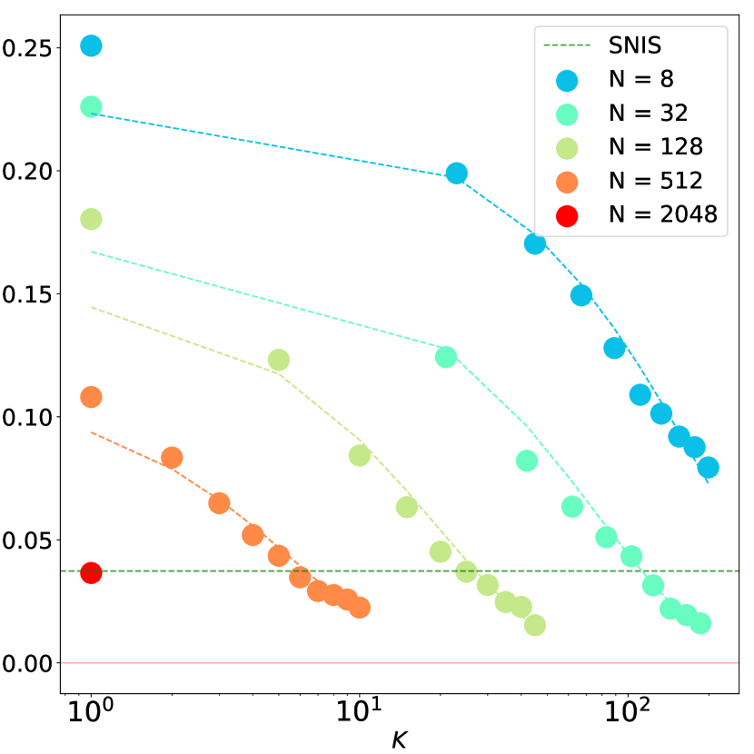
((a)) Bias

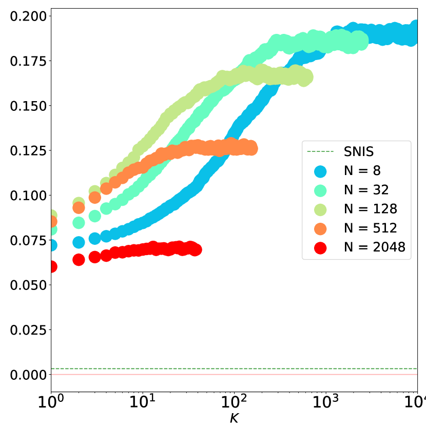
((b)) MSE

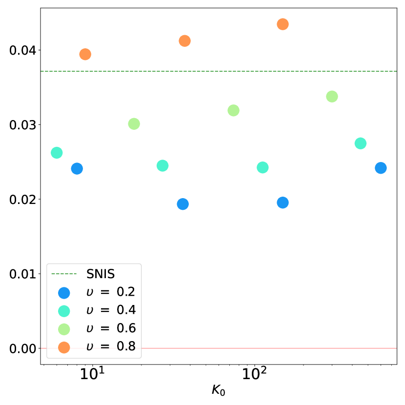
((c)) Rolling bias

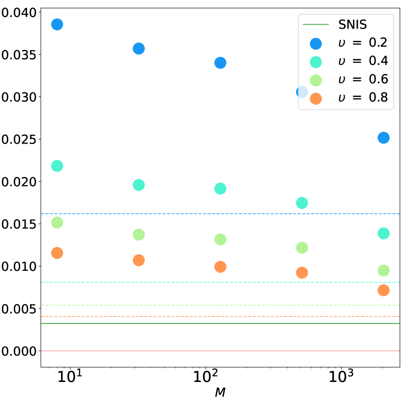
((d)) Rolling MSE

Figure 5: Visualization of the theoretical bounds from Theorems 3 and 4.

Comparison with zero bias SNIS methods:

There exists estimators based on SNIS that have no bias, such as the estimator proposed in [30] and refered to as Unbiased-PIMH . One of the main differences between such estimator and BR-SNIS is that BR-SNIS works under a pre-established budget of samples, whereas in Unbiased-PIMH the number of samples used to produce an estimate varies due to the accept-reject procedure. Even though the two estimators have different goals, it can be of interest to compare both of them in the case where there is a restriction in the total number of samples available.

We proceed to a fixed-budget ($M$) comparison between BR-SNIS and the "Rao Blackwellized" version of the algorithm proposed at [30] in the Gaussian Mixture example. In order to do so, it’s necessary to impose the fixed-budget constraint to the Unbiased-PIMH estimator. A single iteration of the estimator from Unbiased-PIMH with batch-size $N$ needs $rN$ samples where $r\in\mathbb{N}$ is a random number satisfying $r\geq 2$. Therefore, there are two ways of applying the constraint to Unbiased-PIMH :

• Soft: For a given $N$, generate estimations using Unbiased-PIMH until the number of samples is larger than $M$ and keep the last estimation. Therefore, all the estimators from Unbiased-PIMH will have used at least $M$ samples. All the estimations generated are averaged to generate a single estimate.

• Hard: For a given $N$, generate estimations using Unbiased-PIMH until the number of total samples used is larger than $M$ and discard the last estimation. Therefore, all the estimators from Unbiased-PIMH will have used at most $M$ samples. If no estimations were produced under the budget cap (first iteration used more than $M$ samples), then we consider it a miss. All the estimations generated are averaged to create a single estimate.

The code used to run the experiments is available at . For both cases, the following values of $M$ are used in the comparison: $2^{16},2^{12},2^{9}$. For each estimator, a total of $1024$ Monte Carlo replications are used to estimate the mean and the standard deviation of the estimator. Note that in the Hard framework, it can happen that less than 1024 replications are used for the Unbiased-PIMH estimator. The number of failed estimations is reported in the tables for the framework Hard for each configuration.

For each configuration of the BR-SNIS estimator (defined by $N$, $k_{\scriptsize{\mbox{{\it max}}}}$), we have used $90\%$ burn-in period (${k}_{0}=\lfloor 0.9k_{\scriptsize{\mbox{{\it max}}}}\rfloor)$ and $k_{\scriptsize{\mbox{{\it max}}}}$ rounds of bootstrap ($k_{\scriptsize{\mbox{{\it max}}}}$ permutations of the input samples).

The following values were calculated:

• Bias: The mean of the estimations minus $\operatorname{ref}$ over $1024$ replications

• Std: The standard deviation of the estimations over $1024$ replications.

• Fails: The number of replications that failed to produce a single estimation for a given budget $M$. This is only applicable for the Unbiased-PIMH estimator and in the Hard framework.

• average M: The average (over the $1024$ replications) total cost of the estimator. For BR-SNIS and SNIS this is always $M$. For Unbiased-PIMH in the Soft framework it is larger than $M$. In the Hard framework it is smaller than $M$.

Data: $N\geq 0$

$e_{1},\operatorname{lwav}_{1}\leftarrow\mbox{SNIS}{}(N)$ ;

  /* SNIS also returning the average log weights */

1 $e_{2},\operatorname{lwav}_{2}\leftarrow\mbox{SNIS}{}(N)$;

2 if $\operatorname{lwav}_{1}<\operatorname{lwav}_{2}$ then

3       $\operatorname{swap}(e_{1},\operatorname{lwav}_{1};e_{2},\operatorname{lwav}_{2})$

4 end if

5$u=\log\operatorname{rand}()$ ;

6 if $u<\operatorname{lwav}_{1}$ and $u<\operatorname{lwav}_{2}$ then

7       $\tau=1$;

8      

9 end if

10$t\leftarrow 1$;

11 $\tau=\infty$;

12 while $\tau=\infty$ do

13       $e_{1}=e_{1}+(e_{1}-e_{2})$ ;

14       $e_{p},\operatorname{lwav}_{p}=\mbox{SNIS}{}(N)$;

15       $t=t+1$;

16       $u=\log\operatorname{rand}()$; if $u<\operatorname{lwav}_{p}-\operatorname{lwav}_{1}$ then

17             $e_{1},\operatorname{lwav}_{1}=e_{p},\operatorname{lwav}_{p}$;

18            

19       end if

20      

21      if $u<\operatorname{lwav}_{p}-\operatorname{lwav}_{1}$ then

22             $e_{2},\operatorname{lwav}_{1}=e_{p},\operatorname{lwav}_{p}$;

23            

24       end if

25      if $u<\operatorname{lwav}_{1}$ and $u<\operatorname{lwav}_{2}$ then

26             $\tau=t$;

27            

28       end if

29      

30 end while

Algorithm 1 Unbiased-PIMH

comparison_pimh_16comparison_pimh_67108864.csv

N	k	algorithm	Bias	std	average M

Table 3: $M=2^{16}$ in the Soft framework.

comparison_pimh_12comparison_pimh_4194304.csv

N	k	algorithm	Bias	std	average M

Table 4: $M=2^{12}$ in the Soft framework.

comparison_pimh_9comparison_pimh_524288.csv

N	k	algorithm	Bias	std	average M

Table 5: $M=2^{9}$ in the Soft framework.

comparison_pimh_16_mechantcomparison_pimh_67108864_mechant.csv

N	k	algorithm	Bias	std	average M	Fails

Table 6: $M=2^{16}$ in the Hard framework.

comparison_pimh_12_mechantcomparison_pimh_4194304_mechant.csv

N	k	algorithm	Bias	std	average M	Fails

Table 7: $M=2^{12}$ in the Hard framework.

comparison_pimh_9_mechantcomparison_pimh_524288_mechant.csv

N	k	algorithm	Bias	std	average M	Fails

Table 8: $M=2^{9}$ in the Hard framework.

We have compared both estimators in two different frameworks (Hard and Soft) with three different budgets $M=2^{16}$ (tables 6 and 3), $M=2^{12}$ (tables 7 and 4) and $M=2^{9}$ (tables 8 and 5). We observed that in general the BR-SNIS estimator has smaller standard deviation, with the difference of standard deviation being important for the smaller budgets (3 times less for $M=2^{12}$ and 10 times less for $M=2^{9}$ in the Soft framework).

For the Hard framework, we can see that the empirical bias of BR-SNIS is always at most equal to the empirical bias of Unbiased-PIMH . For the Soft framework, we observed that for $M=2^{16}$ that both methods have similar performance, with BR-SNIS having negligible bias in this setting. For $M=2^{12}$ and $M=2^{9}$, BR-SNIS has in general a smaller empirical biais and the standard deviation of Unbiased-PIMH is considerably higher.

C.2 Bayesian Logistic regression

The importance distribution used in the Bayesian logistic regression example is given by the mean-field variational distribution [6]. More precisely, given the target $\pi$ given in Section 3, the proposal $\lambda$ is a Gaussian distribution with mean $\mu$ and diagonal covariance $\operatorname{diag}(\sigma)$, where $\mu,\sigma$ are learnt by maximization of the Evidence Lower Bound (ELBO):

$$\mathcal{L}(\mu,\sigma)=\int\log(\pi(\theta)/\lambda(\theta))\lambda(\theta)\mathrm{d}\theta.$$ (116)

In both Figures 6 and 3, the optimal ${k}$ for a given budget $M$ was chosen by grid search over all the factors of $M$. The final settings are shown in Section C.2. optimal_confsoptimal_config_bayesian_logistic.csv

Dataset	component	M	$k_{\scriptsize{\mbox{{\it max}}}}$	N
*optimal_confs=Dataset,=component, =M, =̨k, =N			˛

Table 9: Optimal configurations for Figures 6 and 3

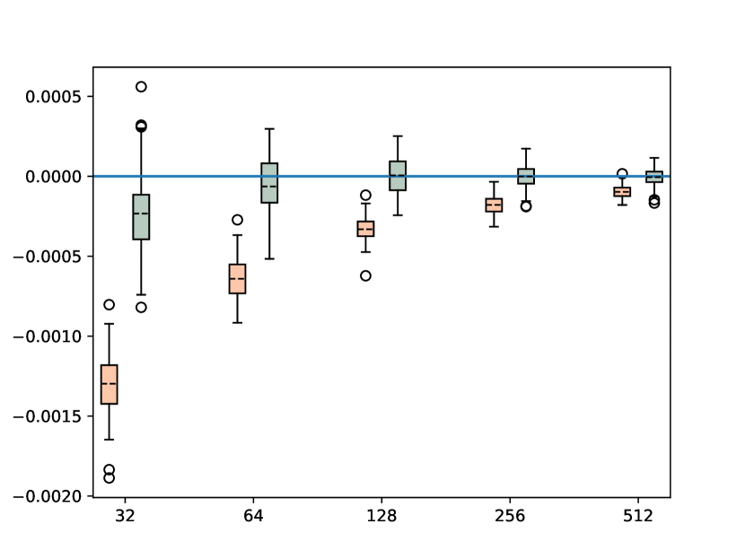
((a)) Heart 5

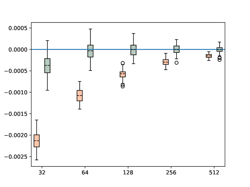
((b)) Heart 12

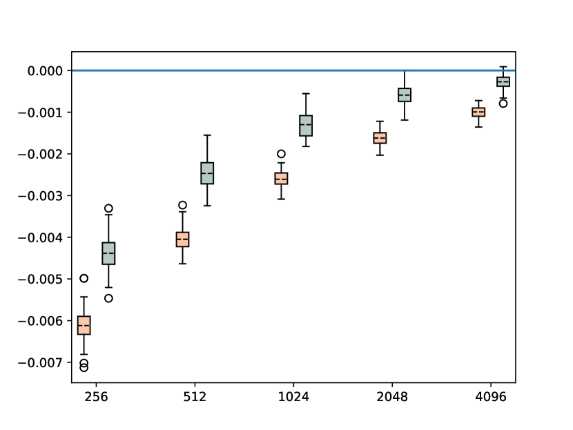
((c)) Breast 8

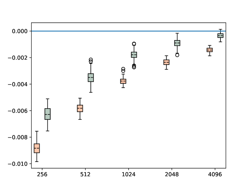
((d)) Breast 14

((e)) Covertype 17

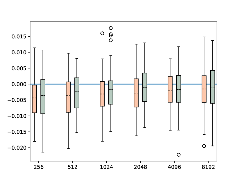
((f)) Covertype 23

Figure 6: Visualisation of the distribution of the bias for the Heart Failure and Breast cancer dataset for other components of $\theta$

C.3 Importance Weighted Auto-Encoders

The details of training procedure are given in Table 10. The train ELBO for each latent dimension is shown in Figure 9. For each network we display generated images in Figures 7 and 8. The generation is done by sampling from the prior $p_{\theta}$.

For the log likelihood comparison in Table 2, we use SNIS with the posterior as importance distribution and a total of $10^{4}$ samples. Therefore, the estimation of the log likelihood is:

$$\hat{\mathcal{L}}=T^{-1}\sum_{j=1}^{T}\sum_{i=1}^{M}\omega_{\theta,\phi,x_{j}}\log p_{\theta}(x_{j}\mid z^{j}_{i})$$ (117)

with $\omega_{\theta,\phi,x}(z)=p_{\theta}(x)/q_{\phi}(z\mid x)$ where $z_{i}^{j}$ is sampled from $q_{\phi}(\cdot\mid x_{j})$.

Name	Value	Name	Value
Batch size	32	Epochs	100
IS samples(IWAE, Un IWAE)	64	Encoder inner layer size	256
Learning rate	$10^{-3}$	Decoder inner layer size	256

Table 10: Training Parameters

((a)) VAE

((b)) IWAE

((c)) Un-IWAE ($k=4$)

((d)) Un-IWAE ($k=8$)

Figure 7: Images generated by the autoencoders from a sample of the prior in the latent space for dimension $20$.

((a)) VAE

((b)) IWAE

((c)) Un-IWAE ($k=4$)

((d)) Un-IWAE ($k=8$)

Figure 8: Images generated by the autoencoders from a sample of the prior in the latent space for dimension $50$.

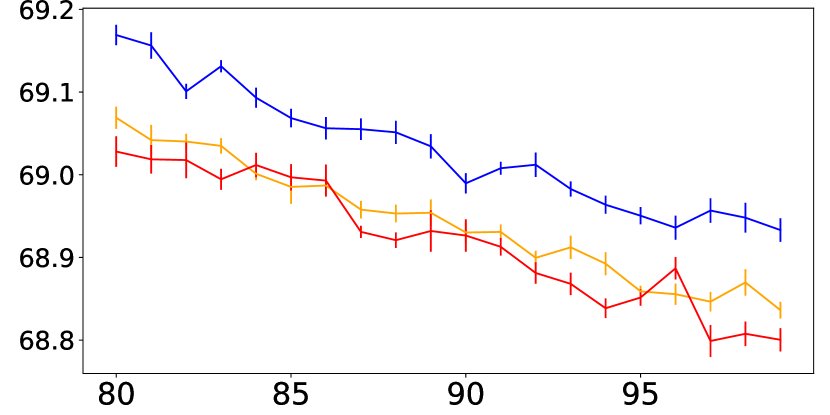
((a)) Dimension 20

((b)) Dimension 50

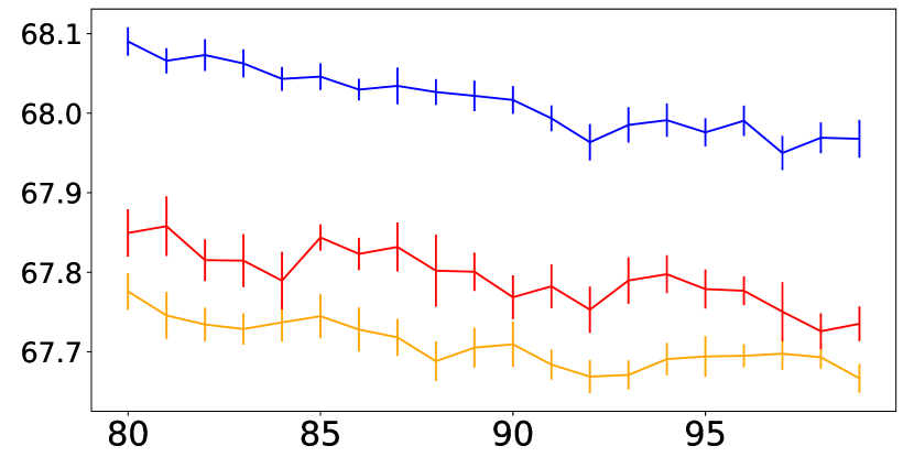
((c)) Dimension 100

Figure 9: Per epoch training loss (ELBO) for the last 25 epochs. Confidence intervals are calculated as $1.96\sigma/\sqrt{n}$ over 4 ($n=4$) different seeds. Blue corresponds to IWAE, orange to BR-IWAE with $k=4$ and red to BR-IWAE with $k=8$.

C.4 Resources

All the simulations were done using a server with the following configuration:

• GPUs: two Tesla V100-PCIE (32Gb RAM)

• CPU: 71 Intel(R) Xeon(R) Gold 6154 CPU @ 3.00GHz

• RAM: 377Gb

locally hosted. We estimate the total number of computing hours for the results presented in this paper to be inferior to 200 hours of GPU usage (All the calculations were done in the GPU).

References

- [1] S. Agapiou, O. Papaspiliopoulos, D. Sanz-Alonso, and A. M. Stuart. Importance sampling: Intrinsic dimension and computational cost. Statistical Science, 32(3):405–431, 2017.
- [2] D. Aldous, L. Lovász, and P. Winkler. Mixing times for uniformly ergodic markov chains. Stochastic Processes and their Applications, 71(2):165–185, 1997.
- [3] C. Andrieu. On random-and systematic-scan samplers. Biometrika, 103(3):719–726, 2016.
- [4] C. Andrieu, A. Doucet, and R. Holenstein. Particle Markov chain Monte Carlo methods. Journal of the Royal Statistical Society: Series B, 72(3):269–342, 2010.
- [5] C. Andrieu, A. Lee, and M. Vihola. Uniform ergodicity of the iterated conditional smc and geometric ergodicity of particle gibbs samplers. Bernoulli, 24(2):842–872, 2018.
- [6] D. M. Blei, A. Kucukelbir, and J. D. McAuliffe. Variational inference: A review for statisticians. Journal of the American statistical Association, 112(518):859–877, 2017.
- [7] N. Bonneel, J. Rabin, G. Peyré, and H. Pfister. Sliced and Radon Wasserstein Barycenters of Measures. Journal of Mathematical Imaging and Vision, 1(51):22–45, 2015.
- [8] Y. Burda, R. Grosse, and R. Salakhutdinov. Importance weighted autoencoders. arXiv preprint arXiv:1509.00519, 2015.
- [9] J. Chen, D. Lian, B. Jin, X. Huang, K. Zheng, and E. Chen. Fast variational autoencoder with inverted multi-index for collaborative filtering. In Proceedings of the ACM Web Conference 2022, pages 1944–1954, 2022.
- [10] R. Douc, E. Moulines, P. Priouret, and P. Soulier. Markov chains. Springer Series in Operations Research and Financial Engineering. Springer, Cham, 2018.
- [11] V. Elvira and L. Martino. Advances in importance sampling. arXiv preprint arXiv:2102.05407, 2021.
- [12] T. Hesterberg. Weighted average importance sampling and defensive mixture distributions. Technometrics, 37(2):185–194, 1995.
- [13] M. D. Hoffman, A. Gelman, et al. The no-U-turn sampler: adaptively setting path lengths in Hamiltonian Monte Carlo. J. Mach. Learn. Res., 15(1):1593–1623, 2014.
- [14] D. Hsu, A. Kontorovich, D. A. Levin, Y. Peres, C. Szepesvári, and G. Wolfer. Mixing time estimation in reversible markov chains from a single sample path. The Annals of Applied Probability, 29(4):2439–2480, 2019.
- [15] H. Kahn and A. W. Marshall. Methods of reducing sample size in monte carlo computations. Journal of the Operations Research Society of America, 1(5):263–278, 1953.
- [16] A. Karbalayghareh, X. Qian, and E. R. Dougherty. Optimal bayesian transfer learning. IEEE Transactions on Signal Processing, 66(14):3724–3739, 2018.
- [17] D. P. Kingma and J. Ba. Adam: A method for stochastic optimization. In ICLR 2015, 2015.
- [18] D. P. Kingma and M. Welling. Stochastic gradient vb and the variational auto-encoder. In Second International Conference on Learning Representations, ICLR, volume 19, page 121, 2014.
- [19] D. P. Kroese and R. Y. Rubinstein. Monte carlo methods. Wiley Interdisciplinary Reviews: Computational Statistics, 4(1):48–58, 2012.
- [20] I. Kuzborskij, C. Vernade, A. Gyorgy, and C. Szepesvári. Confident off-policy evaluation and selection through self-normalized importance weighting. In International Conference on Artificial Intelligence and Statistics, pages 640–648. PMLR, 2021.
- [21] R. Lamberti, Y. Petetin, F. Septier, and F. Desbouvries. A double proposal normalized importance sampling estimator. In 2018 IEEE Statistical Signal Processing Workshop (SSP), pages 238–242. IEEE, 2018.
- [22] J. Lawson, G. Tucker, B. Dai, and R. Ranganath. Energy-inspired models: Learning with sampler-induced distributions. Advances in Neural Information Processing Systems, 32, 2019.
- [23] A. Lee. On auxiliary variables and many-core architectures in computational statistics. PhD thesis, University of Oxford, 2011.
- [24] A. Lee, C. Yau, M. B. Giles, A. Doucet, and C. C. Holmes. On the utility of graphics cards to perform massively parallel simulation of advanced Monte Carlo methods. Journal of computational and graphical statistics, 19(4):769–789, 2010.
- [25] F. Lindsten, R. Douc, and E. Moulines. Uniform ergodicity of the particle gibbs sampler. Scandinavian Journal of Statistics, 42(3):775–797, 2015.
- [26] F. Lindsten, M. I. Jordan, and T. B. Schön. Particle gibbs with ancestor sampling. 2014.
- [27] J. S. Liu, W. H. Wong, and A. Kong. Covariance structure of the gibbs sampler with applications to the comparisons of estimators and augmentation schemes. Biometrika, 81(1):27–40, 1994.
- [28] O. Maddouri, X. Qian, F. J. Alexander, E. R. Dougherty, and B.-J. Yoon. Robust importance sampling for error estimation in the context of optimal bayesian transfer learning. Patterns, page 100428, 2022.
- [29] A. M. Metelli, M. Papini, F. Faccio, and M. Restelli. Policy optimization via importance sampling. Advances in Neural Information Processing Systems, 31, 2018.
- [30] L. Middleton, G. Deligiannidis, A. Doucet, and P. E. Jacob. Unbiased smoothing using particle independent metropolis-hastings. In K. Chaudhuri and M. Sugiyama, editors, Proceedings of the Twenty-Second International Conference on Artificial Intelligence and Statistics, volume 89 of Proceedings of Machine Learning Research, pages 2378–2387. PMLR, 16–18 Apr 2019.
- [31] C. Naesseth, F. Lindsten, and D. Blei. Markovian score climbing: Variational inference with kl (p|| q). Advances in Neural Information Processing Systems, 33:15499–15510, 2020.
- [32] C. A. Naesseth, F. Lindsten, T. B. Schön, et al. Elements of sequential monte carlo. Foundations and Trends® in Machine Learning, 12(3):307–392, 2019.
- [33] R. M. Neal et al. Mcmc using hamiltonian dynamics. Handbook of markov chain monte carlo, 2(11):2, 2011.
- [34] M. Niknejad, J. Bioucas-Dias, and M. A. Figueiredo. External patch-based image restoration using importance sampling. IEEE Transactions on Image Processing, 28(9):4460–4470, 2019.
- [35] D. Paulin. Concentration inequalities for markov chains by marton couplings and spectral methods. Electronic Journal of Probability, 20:1–32, 2015.
- [36] C. Robert and G. Casella. Monte Carlo statistical methods. Springer Science & Business Media, 2013.
- [37] D. B. Rubin. Comment: A noniterative Sampling/Importance Resampling alternative to the data augmentation algorithm for creating a few imputations when fractions of missing information are modest: The SIR algorithm. Journal of the American Statistical Association, 82(398):542–543, 1987.
- [38] R. Salakhutdinov and I. Murray. On the quantitative analysis of deep belief networks. In Proceedings of the 25th international conference on Machine learning, pages 872–879, 2008.
- [39] T. Schwedes and B. Calderhead. Rao-blackwellised parallel mcmc. In A. Banerjee and K. Fukumizu, editors, Proceedings of The 24th International Conference on Artificial Intelligence and Statistics, volume 130 of Proceedings of Machine Learning Research, pages 3448–3456. PMLR, 13–15 Apr 2021.
- [40] A. Swaminathan and T. Joachims. The self-normalized estimator for counterfactual learning. advances in neural information processing systems, 28, 2015.
- [41] A. Thin, Y. Janati El Idrissi, S. Le Corff, C. Ollion, E. Moulines, A. Doucet, A. Durmus, and C. X. Robert. Neo: Non equilibrium sampling on the orbits of a deterministic transform. Advances in Neural Information Processing Systems, 34:17060–17071, 2021.
- [42] H. Tjelmeland. Using all Metropolis–Hastings proposals to estimate mean values. Technical report, 2004.
- [43] H. Tjelmeland. Using all metropolis-hastings proposals to estimate mean values. 2004.
- [44] R. Vershynin. High-dimensional probability: An introduction with applications in data science, volume 47. Cambridge university press, 2018.
- [45] M. J. Wainwright. High-dimensional statistics: A non-asymptotic viewpoint, volume 48. Cambridge University Press, 2019.