Iterative Linear Quadratic Optimization for Nonlinear Control:
Differentiable Programming Algorithmic Templates

Abstract

We present the implementation of nonlinear control algorithms based on linear and quadratic approximations of the objective from a functional viewpoint. We present a gradient descent, a Gauss-Newton method, a Newton method, differential dynamic programming approaches with linear quadratic or quadratic approximations, various line-search strategies, and regularized variants of these algorithms. We derive the computational complexities of all algorithms in a differentiable programming framework and present sufficient optimality conditions. We compare the algorithms on several benchmarks, such as autonomous car racing using a bicycle model of a car. The algorithms are coded in a differentiable programming language in a publicly available package.

1 Introduction

We consider nonlinear control problems in discrete time with finite horizon, i.e., problems of the form

$$\min_{\begin{subarray}{c}x_{0},\ldots,x_{\tau}\in{\mathbb{R}}^{n_{x}}\\ u_{0}\ldots,u_{\tau-1}\in{\mathbb{R}}^{n_{u}}\end{subarray}} \sum_{t=0}^{\tau-1}h_{t}(x_{t},u_{t})+h_{\tau}(x_{\tau})$$ (1)

subject to $$x_{t+1}=f_{t}(x_{t},u_{t}),\quad\mbox{for}\ t\in\{0,\ldots,\tau-1\},\quad x_{0}=\bar{x}_{0},$$

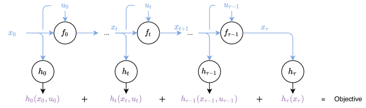
Figure 1: Computational scheme of the discrete time control problem (1).

where at time $t$, $x_{t}\in{\mathbb{R}}^{{n_{x}}}$ is the state of the system, $u_{t}\in{\mathbb{R}}^{n_{u}}$ is the control applied to the system, $f_{t}:{\mathbb{R}}^{n_{x}}\times{\mathbb{R}}^{n_{u}}\rightarrow{\mathbb{R}}^{n_{x}}$ is the discrete dynamic, $h_{t}:{\mathbb{R}}^{n_{x}}\rightarrow{\mathbb{R}}$ is the cost on the state and control variables and $\bar{x}_{0}\in{\mathbb{R}}^{n_{x}}$ is a given fixed initial state. Problem (1) is entirely determined by the initial state and the controls as illustrated in Fig. 1.

Problems of the form (1) have been tackled in various ways, from direct approaches using nonlinear optimization (Betts,, 2010; Wright,, 1990; Wright, 1991a, ; Pantoja,, 1988; Dunn and Bertsekas,, 1989; Rao et al.,, 1998) to convex relaxations using semidefinite optimization (Boyd and Vandenberghe,, 1997). A popular approach of the former category proceeds by computing at each iteration the linear quadratic regulator associated with a linear quadratic approximation of the problem around the current candidate solutions (Jacobson and Mayne,, 1970; Li and Todorov,, 2007; Sideris and Bobrow,, 2005; Tassa et al.,, 2012). The computed feedback policies are then applied either along the linearized dynamics or along the original dynamics to output a new candidate solution.

We present the algorithmic implementation of such approaches, from the computational complexities of the optimization oracles to various implementations of line-search procedures. By considering these algorithms from a functional viewpoint, we delineate the discrepancies between the different algorithms and identify the common subroutines. We review the implementation of (i) a Gauss-Newton method (Sideris and Bobrow,, 2005), (ii) a Newton method (Pantoja,, 1988; Liao and Shoemaker,, 1991; Dunn and Bertsekas,, 1989), (iii) a Differential Dynamic Programming (DDP) approach based on linear approximations of the dynamics and quadratic approximations of the costs (Tassa et al.,, 2012), (iv) a DDP approach based on quadratic approximations of both dynamics and costs (Jacobson and Mayne,, 1970). We also consider regularized variants of the aforementioned algorithms with their corresponding line-searches. In addition, we present simple formulations of the gradient and the Hessian of the overall objective w.r.t. the control variables that can be used to estimate the smoothness properties of the objective. We also recall necessary optimality conditions for problem (1), present a counterexample of why Pontryagin’s maximum principle (Pontryagin et al.,, 1963) does not apply in discrete time, and present sufficient optimality conditions derived from the continuous counterpart of the problem. Finally, we present numerical comparisons of the algorithms and their variants on several control tasks such as autonomous car racing.

Related work

The idea of tackling nonlinear control problems of the form (1) by minimizing linear quadratic approximations of the problem is at least 50 years old (Jacobson and Mayne,, 1970). One of the first approaches consisted of a Differential Dynamic Programming (DDP) approach using quadratic approximations as presented by Jacobson and Mayne, (1970) and further explored by Mayne and Polak, (1975); Murray and Yakowitz, (1984); Liao and Shoemaker, (1991). An implementation of a Newton method for nonlinear control problems of the form (1) was developed after the DDP approach by Pantoja, (1988); Dunn and Bertsekas, (1989). A parallel implementation of a Newton step and sequential quadratic programming methods were developed by Wright, (1990); Wright, 1991a , which led to efficient implementations of interior point methods for linear quadratic control problems under constraints by using the block band diagonal structure of the system of KKT equations solved at each step (Wright, 1991b, ). A detailed comparison of the DDP approach and the Newton method was conducted by Liao and Shoemaker, (1992), who observed that the original DDP approach generally outperforms its Newton counterpart. We extend this analysis by comparing regularized variants of the algorithms. Finally, the storage of second order information for DDP and Newton can be alleviated with a careful implementation in a differentibale programming framework as done in our implementation and noted earlier by Nganga and Wensing, (2021).

Simpler approaches consisting in taking linear approximations of the dynamics and quadratic approximations of the costs were implemented as part of public software (Todorov et al.,, 2012). The resulting Iterative Linear Quadratic Regulator algorithm as formulated by Li and Todorov, (2007) amounts naturally to a Gauss-Newton method (Sideris and Bobrow,, 2005). A variant that mixes linear quadratic approximations of the problem with a DDP approach was further analyzed empirically by Tassa et al., (2012). Here, we detail the line-searches for both approaches and present their regularized variants. We provide detailed computational complexities of all aforementioned algorithms that illustrate the trade-offs between the approaches.

Our derivations are based on the decomposition of the first and second derivatives of the problem in a compact formulation that can be used to, e.g., estimate the smoothness properties of the problem in a straightforward way. We also present sufficient optimality conditions of a candidate solution for problem (1) by translating sufficient conditions developed in continuous time by Arrow, (1968); Mangasarian, (1966); Kamien and Schwartz, (1971).

For our experiments, we adapted the bicycle model of a miniature car developed by Liniger et al., (2015) in Python. We provide an implementation in Python, available at https://github.com/vroulet/ilqc for further exploration of the algorithms. This work also serves as a companion reference for the convergence analysis of iterative linear quadratic optimization algorithms for nonlinear control by the same authors (Roulet et al.,, 2022).

Outline

In Sec. 2 we recall how linear quadratic control problems are solved by dynamic programming and how the linear quadratic case serves as a building block for nonlinear control algorithms. Sec. 3 presents how first and second order information of the objective can be expressed in terms of the first and second order information of the dynamics. The implementation of classical optimization oracles such as a gradient step, a Gauss-Newton step or a Newton step is presented in Sec. 4. Sec 5 details the rationale and the implementation of differential dynamic programming approaches. Sec. 6 details the line-search procedures. Sec. 7 presents the computational complexities of each oracle in terms of space and time complexities in a differentiable programming framework. We recall necessary optimality conditions for problem (1) and present sufficient optimality conditions in Sec. 8. A summary of all algorithms with detailed pseudocode and computational schemes is given in Sec. 9. All algorithms are then tested on several synthetic problems in Sec. 10: swinging-up a fixed pendulum, or a pendulum on a cart, and autonomous car racing with simple dynamics or with a bicycle model.

Notations

For a sequence of vectors $x_{1},\ldots,x_{\tau}\in{\mathbb{R}}^{n_{x}}$, we denote by semi-colons their concatenation s.t. ${\bm{x}}=(x_{1};\ldots;x_{\tau})\in{\mathbb{R}}^{\tau{n_{x}}}$. For a function $f:{\mathbb{R}}^{d}\rightarrow{\mathbb{R}}^{n}$, we denote by $\nabla f(x)=(\partial_{x_{i}}f_{j}(x))_{\begin{subarray}{c}1\leq i\leq d,1\leq j\leq n\end{subarray}}\in{\mathbb{R}}^{d\times n}$ the gradient of $f$, i.e., the transpose of the Jacobian of $f$ on $x$. For a function $f:{\mathbb{R}}^{d}\times{\mathbb{R}}^{p}\rightarrow{\mathbb{R}}^{n}$, we denote for $x\in{\mathbb{R}}^{d}$, $y\in{\mathbb{R}}^{p}$, $\nabla_{x}f(x,y)=(\partial_{x_{i}}f_{j}(x,y))_{\begin{subarray}{c}1\leq i\leq d,1\leq j\leq n\end{subarray}}\in{\mathbb{R}}^{d\times n}$ the partial gradient of $f$ w.r.t. $x$ on $(x,y)$. For $f:{\mathbb{R}}^{d}\rightarrow{\mathbb{R}}^{n}$, we denote the Lipschitz continuity constant of $f$ as $l_{f}{=}\sup_{x,y\in{\mathbb{R}}^{d},x\neq y}\|f(x){-}f(y)\|_{2}/\|x{-}y\|_{2}$.

A tensor $\mathcal{A}=(a_{i,j,k})_{1\leq i\leq d,1\leq j\leq p,1\leq k\leq n}\in{\mathbb{R}}^{d\times p\times n}$ is represented as a list of matrices $\mathcal{A}=(A_{1},\ldots,A_{n})$ where $A_{k}=(a_{i,j,k})_{1\leq i\leq d,1\leq j\leq p}\in{\mathbb{R}}^{d\times p}$ for $k\in\{1,\ldots n\}$. Given $\mathcal{A}\in{\mathbb{R}}^{d\times p\times n}$ and $P\in{\mathbb{R}}^{d\times d^{\prime}},Q\in{\mathbb{R}}^{p\times p^{\prime}},R\in{\mathbb{R}}^{n\times n^{\prime}}$, we denote $\mathcal{A}[P,Q,R]=\left(\sum_{k=1}^{n}R_{k,1}P^{\top}A_{k}Q,\ldots,\sum_{k=1}^{n}R_{k,n^{\prime}}P^{\top}A_{k}Q\right)\in{\mathbb{R}}^{d^{\prime}\times p^{\prime}\times n^{\prime}}.$ For $\mathcal{A}_{0}\in{\mathbb{R}}^{d_{0}\times p_{0}\times n_{0}}$, $P\in{\mathbb{R}}^{d_{0}\times d_{1}},Q\in{\mathbb{R}}^{p_{0}\times p_{1}},R\in{\mathbb{R}}^{n_{0}\times n_{1}}$ denote $\mathcal{A}_{1}=\mathcal{A}_{0}[P,Q,R]\in{\mathbb{R}}^{d_{1}\times p_{1}\times n_{1}}$. Then, for $S\in{\mathbb{R}}^{d_{1}\times d_{2}},T\in{\mathbb{R}}^{p_{1}\times p_{2}},U\in{\mathbb{R}}^{n_{1}\times n_{2}}$, we have $\mathcal{A}_{1}[S,T,U]=\mathcal{A}_{0}[PS,QT,RU]\in{\mathbb{R}}^{d_{2}\times p_{2}\times n_{2}}.$ If $P,Q$ or $R$ are identity matrices, we use the symbol “$\>\cdot\>$” in place of the identity matrix. For example, we denote $\mathcal{A}[P,Q,\operatorname{I}_{n}]=\mathcal{A}[P,Q,\cdot]=\left(P^{\top}A_{1}Q,\ldots,P^{\top}A_{n}Q\right)$. If $P,Q$ or $R$ are vectors we consider the flatten object. In particular, for $x\in{\mathbb{R}}^{d},y\in{\mathbb{R}}^{p}$, we denote $\mathcal{A}[x,y,\cdot]=\left(\begin{matrix}x^{\top}A_{1}y,\ldots,x^{\top}A_{n}y\end{matrix}\right)^{\top}\in{\mathbb{R}}^{n},$ rather than having $\mathcal{A}[x,y,\cdot]\in{\mathbb{R}}^{1\times 1\times n}$. Similarly, for $z\in{\mathbb{R}}^{n}$, we denote $\mathcal{A}[\cdot,\cdot,z]=\sum_{k=1}^{n}z_{k}A_{k}\in{\mathbb{R}}^{d\times p}.$ We denote $\|a\|_{2}$ the Euclidean norm for $a\in{\mathbb{R}}^{d}$, $\|A\|_{2,2}$ the spectral norm of a matrix $A\in{\mathbb{R}}^{d\times p}$ and we define the norm of a tensor $\mathcal{A}$ induced by the Euclidean norm as $\|\mathcal{A}\|_{2,2,2}=\sup_{x\neq 0,y\neq 0,z\neq 0}\mathcal{A}[x,y,z]/(\|x\|_{2}\|y\|_{2}\|z\|_{2}).$

For a multivariate function $f:{\mathbb{R}}^{d}\rightarrow{\mathbb{R}}^{n}$ composed of coordinates $f_{j}:{\mathbb{R}}^{d}\rightarrow{\mathbb{R}}$ for $j\in\{1,\ldots,n\}$, we denote its Hessian $x\in{\mathbb{R}}^{d}$ as a tensor $\nabla^{2}f(x)=(\nabla^{2}f_{1}(x),\ldots,\nabla^{2}f_{n}(x))\in{\mathbb{R}}^{d\times d\times n}$. For a multivariate function $f:{\mathbb{R}}^{d}\times{\mathbb{R}}^{p}\rightarrow{\mathbb{R}}^{n}$ composed of coordinates $f_{j}:{\mathbb{R}}^{d}\times{\mathbb{R}}^{p}\rightarrow{\mathbb{R}}$ for $j\in\{1,\ldots,n\}$, we decompose its Hessian on $x\in{\mathbb{R}}^{d}$, $y\in{\mathbb{R}}^{p}$ by defining, e.g., $\nabla_{xx}^{2}f(x,y)=(\nabla_{xx}^{2}f_{1}(x,y),\ldots,\nabla_{xx}^{2}f_{n}(x,y))\in{\mathbb{R}}^{d\times d\times n}$. The quantities $\nabla_{yy}^{2}f(x,y)\in{\mathbb{R}}^{p\times p\times n},\nabla_{xy}^{2}f(x,y)\in{\mathbb{R}}^{d\times p\times n},\nabla_{yx}^{2}f(x,y)\in{\mathbb{R}}^{p\times d\times n}$ are defined similarly.

For a function $f:{\mathbb{R}}^{d}\rightarrow{\mathbb{R}}^{n}$, and $x\in{\mathbb{R}}^{d}$, we define the finite difference expansion of $f$ around $x$, the linear expansion of $f$ around $x$ and the quadratic expansion of $f$ around $x$ as, respectively,

$$\delta_{f}^{x}(y)=f(x+y)-f(x),\qquad\ell_{f}^{x}(y)=\nabla f(x)^{\top}y,\qquad q_{f}^{x}(y)=\nabla f(x)^{\top}y+\frac{1}{2}\nabla^{2}f(x)[y,y,\cdot].$$ (2)

The linear and quadratic approximations of $f$ around $x$ are then $f(x+y)\approx f(x)+\ell_{f}^{x}(y)$ and $f(x+y)\approx f(x)+q_{f}^{x}(y)$ respectively.

2 From Linear Control Problems to Nonlinear Control Algorithms

Algorithms for nonlinear control problems revolve around the resolution of linear quadratic control problems by dynamic programming. Therefore, we start by recalling the rationale of dynamic programming and how discrete time control problems with linear dynamics and quadratic costs can be solved by dynamic programming.

2.1 Dynamic Programming

The idea of dynamic programming is to decompose dynamical problems such as (1) into a sequence of nested subproblems defined by the cost-to-go from $x_{t}$ at time $t\in\{0,\ldots,\tau-1\}$

$$c_{t}(x_{t})=\min_{\begin{subarray}{c}u_{t},\ldots,u_{\tau-1}\in{\mathbb{R}}^{n_{u}}\\ y_{t},\ldots,y_{\tau}\in{\mathbb{R}}^{n_{x}}\end{subarray}}\quad \sum_{s=t}^{\tau-1}h_{s}(y_{s},u_{s})+h_{\tau}(y_{\tau})$$

subject to $$y_{s+1}=f_{s}(y_{s},u_{s})\quad\mbox{for}\ s\in\{t,\ldots,\tau-1\},\quad y_{t}=x_{t}.$$

The cost-to-go from $x_{\tau}$ at time $\tau$ is simply the last cost, namely, $c_{\tau}(x_{\tau})=h_{\tau}(x_{\tau}),$ and the original problem (1) amounts to compute $c_{0}(\bar{x}_{0})$. The cost-to-go functions define nested subproblems that are linked for $t\in\{0,\ldots,\tau-1\}$ by Bellman’s equation (Bellman,, 1971)

$$c_{t}(x_{t}) =\min_{u_{t}\in{\mathbb{R}}^{n_{u}}}h_{t}(x_{t},u_{t})+\min_{\begin{subarray}{c}u_{t+1},\ldots,u_{\tau-1}\in{\mathbb{R}}^{n_{u}}\\ y_{t+1},\ldots,y_{\tau}\in{\mathbb{R}}^{n_{x}}\end{subarray}}\sum_{s=t+1}^{\tau-1}h_{s}(y_{s},u_{s})+h_{\tau}(y_{\tau})$$

$$\hskip 105.0pt\mbox{subject to}\hskip 20.0pty_{s+1}=f_{s}(y_{s},u_{s})\ \mbox{for}\ s\in\{t+1,\ldots,\tau-1\},\ y_{t+1}=f_{t}(x_{t},u_{t})$$

$$=\min_{u_{t}\in{\mathbb{R}}^{n_{u}}}h_{t}(x_{t},u_{t})+c_{t+1}(f_{t}(x_{t},u_{t})).$$ (3)

The optimal control at time $t$ from state $x_{t}$ is given by $u_{t}=\pi_{t}(x_{t})$, where $\pi_{t}$, called a policy, is given by

$$\pi_{t}(x_{t})=\operatorname*{arg\,min}_{u_{t}\in{\mathbb{R}}^{n_{u}}}\left\{h_{t}(x_{t},u_{t})+c_{t+1}(f_{t}(x_{t},u_{t}))\right\}.$$

Define the procedure that back-propagates the cost-to-go functions as

$$\operatorname{BP}:f_{t},h_{t},c_{t+1}\rightarrow\left(\begin{array}[]{c}c_{t}:x\rightarrow\min_{u\in{\mathbb{R}}^{n_{u}}}\left\{h_{t}(x,u)+c_{t+1}(f_{t}(x,u))\right\},\\ \pi_{t}:x\rightarrow\operatorname*{arg\,min}_{u\in{\mathbb{R}}^{n_{u}}}\left\{h_{t}(x,u)+c_{t+1}(f_{t}(x,u))\right\}\end{array}\right).$$

A dynamic programming approach, formally described in Algo. 1, solves problems of the form (1) as follows.

1. Compute recursively the cost-to-go functions $c_{t}$ for $t=\tau,\ldots,0$ using Bellman’s equation (2.1), i.e., compute from $c_{\tau}=h_{\tau}$,

   $$c_{t},\pi_{t}=\operatorname{BP}(f_{t},h_{t},c_{t+1})\quad\mbox{for}\ t\in\{\tau-1,\ldots,0\},$$

   and record at each step the policies $\pi_{t}$.

2. Unroll the optimal trajectory that starts from time 0 at $\bar{x}_{0}$, follows the dynamics $f_{t}$, and uses at each step the optimal control given by the computed policies, i.e., starting from $x_{0}^{*}=\bar{x}_{0}$, compute

   $$u^{*}_{t}=\pi_{t}(x_{t}^{*}),\qquad x_{t+1}^{*}=f_{t}(x_{t}^{*},u^{*}_{t})\qquad\mbox{for $t=0,\ldots,\tau-1$.}$$ (4)

The resulting command ${\bm{u}}^{*}=(u_{0}^{*};\ldots;u_{\tau-1}^{*})$ and trajectory ${\bm{x}}^{*}=(x_{1}^{*};\ldots;x_{\tau}^{*})$ are then optimal for problem (1). In the following, we consider Algo. 1 as a procedure

$$\operatorname{DynProg}:(f_{t})_{t=0}^{\tau-1},(h_{t})_{t=0}^{\tau},\bar{x}_{0},\operatorname{BP}\rightarrow u_{0}^{*},\ldots,u_{\tau-1}^{*}.$$

The bottleneck of the approach is the ability to solve Bellman’s equation (2.1), i.e., having access to the procedure $\operatorname{BP}$ defined above.

Algorithm 1 Dynamic programming procedure
                                                                                                                                    $\left[\operatorname{DynProg}:(f_{t})_{t=0}^{\tau-1},(h_{t})_{t=0}^{\tau},\bar{x}_{0},\operatorname{BP}\rightarrow(u^{*}_{0};\ldots;u^{*}_{\tau-1})\right]$.

1:Inputs: Dynamics $(f_{t})_{t=0}^{\tau-1}$, costs $(h_{t})_{t=0}^{\tau}$, initial state $\bar{x}_{0}$, procedure $\operatorname{BP}$

2:Initialize $c_{\tau}=h_{\tau}$

3:for $t=\tau-1,\ldots,0$ do

4:     Compute $c_{t},\pi_{t}=\operatorname{BP}(f_{t},h_{t},c_{t+1})$, store $\pi_{t}$ $\triangleright$ $\operatorname{BP}=\operatorname{LQBP}$ (Algo. 2) for linear quadratic control

5:end for

6:Initialize $x_{0}^{*}=\bar{x}_{0}$

7:for $t=0,\ldots,\tau-1$ do

8:     Compute $u_{t}^{*}=\pi_{t}(x_{t}^{*})$, $x_{t+1}^{*}=f_{t}(x_{t}^{*},u_{t}^{*})$

9:end for

10:Output: Optimal command ${\bm{u}}=(u_{0}^{*};\ldots;u_{\tau-1}^{*})$ for problem (1)

2.2 Linear Dynamics, Quadratic Costs

For linear dynamics and quadratic costs, problem (1) takes the form

$$\min_{\begin{subarray}{c}x_{0},\ldots,x_{\tau}\in{\mathbb{R}}^{n_{x}}\\ u_{0}\ldots,u_{\tau-1}\in{\mathbb{R}}^{n_{u}}\end{subarray}} \sum_{t=0}^{\tau-1}\left(\frac{1}{2}x_{t}^{\top}P_{t}x_{t}+\frac{1}{2}u_{t}^{\top}Q_{t}u_{t}+x_{t}^{\top}R_{t}u_{t}+p_{t}^{\top}x_{t}+q_{t}^{\top}u_{t}\right)+\frac{1}{2}x_{\tau}^{\top}P_{\tau}x_{\tau}+p_{\tau}^{\top}x_{\tau}$$

subject to $$x_{t+1}=A_{t}x_{t}+B_{t}u_{t},\quad\mbox{for}\ t\in\{0,\ldots,\tau-1\},\quad x_{0}=\bar{x}_{0}.$$

Namely, we have $h_{t}(x_{t},u_{t})=\frac{1}{2}x_{t}^{\top}P_{t}x_{t}+\frac{1}{2}u_{t}^{\top}Q_{t}u_{t}+x_{t}^{\top}R_{t}u_{t}+p_{t}^{\top}x_{t}+q_{t}^{\top}u_{t}$ and $f_{t}(x_{t},u_{t})=A_{t}x_{t}+B_{t}u_{t}$. In that case, under appropriate conditions on the quadratic functions, Bellman’s equation (2.1) can be solved analytically as recalled in Lemma 2.1. Note that the operation $\operatorname{LQBP}$ defined in (5) amounts to computing the Schur complement of a block of the Hessian of the quadratic $x,u\rightarrow q_{t}(x,u)+c_{t+1}(\ell_{t}(x,u))$, namely, the block corresponding to the Hessian w.r.t. the control variables.

Lemma 2.1.

The back-propagation of cost-to-go functions for linear dynamics and quadratic costs is implemented in Algo. 2 which computes

$$\operatorname{LQBP}:(\ell_{t},q_{t},c_{t+1})\rightarrow\left(\begin{array}[]{c}c_{t}:x\rightarrow\min_{u\in{\mathbb{R}}^{n_{u}}}\left\{q_{t}(x,u)+c_{t+1}(\ell_{t}(x,u))\right\}\\ \pi_{t}:x\rightarrow\operatorname*{arg\,min}_{u\in{\mathbb{R}}^{n_{u}}}\left\{q_{t}(x,u)+c_{t+1}(\ell_{t}(x,u))\right\}\end{array}\right),$$ (5)

for linear functions $\ell_{t}$ and quadratic functions $q_{t},c_{t+1}$, s.t. $q_{t}(x,\cdot)+c_{t+1}(\ell_{t}(x,\cdot))$ is strongly convex for any $x$.

Proof.

Consider $\ell_{t},q_{t},c_{t+1}$ to be parameterized as $\ell_{t}(x,u)=Ax+Bu$, $q_{t}(x,u)=\frac{1}{2}x^{\top}Px+\frac{1}{2}u^{\top}Qu+x^{\top}Ru+p^{\top}x+q^{\top}u$, $c_{t+1}(x)=\frac{1}{2}x^{\top}J_{t+1}x+j_{t+1}^{\top}x+j^{0}_{t+1}.$ The cost-to-go function at time $t$ is

$$c_{t}(x) =\frac{1}{2}x^{\top}Px+p^{\top}x+j^{0}_{t+1}$$

$$\quad+\min_{u\in{\mathbb{R}}}\left\{\frac{1}{2}(Ax+Bu)^{\top}J_{t+1}(Ax+Bu)+j_{t+1}^{\top}(Ax+Bu)+\frac{1}{2}u^{\top}Qu+x^{\top}Ru+q^{\top}u\right\}.$$

Since $h(x,\cdot)+c_{t+1}(\ell(x,\cdot))$ is strongly convex, we have that $Q+B^{\top}J_{t+1}B\succ 0$. Therefore, the policy at time $t$ is

$$\pi_{t}(x)=-(Q+B^{\top}J_{t+1}B)^{-1}[(R^{\top}+B^{\top}J_{t+1}A)x+q+B^{\top}j_{t+1}].$$

Using that $\min_{u}u^{\top}Mu/2+m^{\top}x=-m^{\top}M^{-1}m/2$ where, here, $M=Q+B^{\top}J_{t+1}B$, $m=(R^{\top}+B^{\top}J_{t+1}A)x+q+B^{\top}j_{t+1}$, we get that the cost-to-go function at time $t$ is given by

$$c_{t}(x) =\frac{1}{2}x^{\top}\left(P+A^{\top}J_{t+1}A-(R+A^{\top}J_{t+1}B)(Q+B^{\top}J_{t+1}B)^{-1}(R^{\top}+B^{\top}J_{t+1}A)\right)x$$

$$\quad+\left(p+A^{\top}j_{t+1}-(R+A^{\top}J_{t+1}B)(Q+B^{\top}J_{t+1}B)^{-1}(q+B^{\top}j_{t+1})\right)^{\top}x$$

$$\quad-\frac{1}{2}(q+B^{\top}j_{t+1})^{\top}(Q+B^{\top}J_{t+1}B)^{-1}(q+B^{\top}j_{t+1})+j^{0}_{t+1}.$$

∎

If problem (1) consists of linear dynamics and quadratic costs that are strongly convex w.r.t. the control variable, the procedure $\operatorname{LQBP}$ can be applied iteratively in a dynamic programming approach to give the solution of the problem, as formally stated in Corollary 2.2.

Corollary 2.2.

Consider problem (1) such that for all $t\in\{0,\ldots,\tau-1\}$, $f_{t}$ is linear, $h_{t}$ is convex quadratic with $h_{t}(x,\cdot)$ strongly convex for any $x$, and $h_{\tau}$ is convex quadratic. Then, the solution of problem (1) is given by

$${\bm{u}}^{*}=\operatorname{DynProg}((f_{t})_{t=0}^{\tau-1},(h_{t})_{t=0}^{\tau},\bar{x}_{0},\operatorname{LQBP}),$$

with $\operatorname{DynProg}$ implemented in Algo. 1 and $\operatorname{LQBP}$ implemented in Algo. 2

Proof.

Note that at time $t\in\{0,\ldots,\tau-1\}$ for a given $x\in{\mathbb{R}}^{n_{x}}$, if $c_{t+1}$ is convex, then $c_{t+1}(f_{t}(x,\cdot))$ is convex as the composition of a convex function and a linear function and $c_{t+1}(f_{t}(x,\cdot))+h_{t}(x,\cdot)$ is then strongly convex as the sum of a convex and a strongly convex function. Moreover, $x,u\rightarrow c_{t+1}(f_{t}(x,u))+h_{t}(x,u)$ is jointly convex since $x,u\rightarrow c_{t+1}(f_{t}(x,u))$ is the composition of a convex function with a linear function and $h_{t}$ is convex by assumption. Therefore $c_{t}:x\rightarrow\min_{u\in{\mathbb{R}}^{n_{u}}}c_{t+1}(f_{t}(x,u))+h_{t}(x,u)$ is convex as the partial infimum of jointly convex function.

In summary, at time $t\in\{0,\ldots,\tau-1\}$, if $c_{t+1}$ is convex, then (i) $c_{t+1}(f_{t}(x,\cdot))+h_{t}(x,\cdot)$ is strongly convex, and (ii) $c_{t}$ is convex. This ensures that the assumptions of Lemma 2.1 are satisfied at each iteration of Algo. 1 (line 4) since $c_{\tau}=h_{\tau}$ is convex. ∎

2.3 Nonlinear Control Algorithm Example

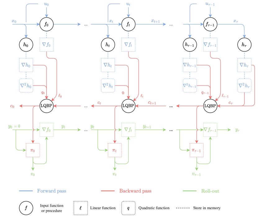
Figure 4: Computational scheme of an ILQR/Gauss-Newton oracle.

Nonlinear control algorithms based on nonlinear optimization use linear or quadratic approximations of the dynamics and the costs at a current candidate sequence of controllers to apply a dynamic programming procedure to the resulting problem. For example, the Iterative Linear Quadratic Regulator (ILQR) algorithm uses linear approximations of the dynamics and quadratic approximations of the costs (Li and Todorov,, 2007). Each iteration of the ILQR algorithm is composed of three steps illustrated in Fig. 4.

Iterative Linear Quadratic Regulator Iteration

1. Forward pass: Given a set of control variables $u_{0},\ldots,u_{\tau-1}$, compute the trajectory $x_{1},\ldots,x_{\tau}$ as $x_{t+1}=f_{t}(x_{t},u_{t})$ starting from $x_{0}=\bar{x}_{0}$, and the associated costs $h_{t}(x_{t},u_{t}),h_{\tau}(x_{\tau})$, for $t\in\{0,\ldots,\tau-1\}$. Record along the computations, i.e., for $t\in\{0,\ldots,\tau-1\}$, the gradients of the dynamics and the gradients and Hessians of the costs.

2. Backward pass: Compute the optimal policies associated with the linear quadratic control problem

   $$\min_{\begin{subarray}{c}y_{0},\ldots y_{\tau}\in{\mathbb{R}}^{n_{x}}\\ v_{0},\ldots,v_{\tau-1}\in{\mathbb{R}}^{n_{u}}\end{subarray}} \sum_{t=0}^{\tau-1}\left(\frac{1}{2}y_{t}^{\top}P_{t}y_{t}+\frac{1}{2}v_{t}^{\top}Q_{t}v_{t}+y_{t}^{\top}R_{t}v_{t}+p_{t}^{\top}y_{t}+q_{t}^{\top}v_{t}\right)+\frac{1}{2}y_{\tau}^{\top}P_{\tau}y_{\tau}+p_{\tau}^{\top}y_{\tau}$$

   subject to $$y_{t+1}=A_{t}y_{t}+B_{t}v_{t},\quad\mbox{for}\ t\in\{0,\ldots,\tau-1\},\quad y_{0}=0,$$

   where $$P_{t}=\nabla_{x_{t}x_{t}}^{2}h_{t}(x_{t},u_{t})\ \ Q_{t}=\nabla_{u_{t}u_{t}}^{2}h_{t}(x_{t},u_{t})\ \ R_{t}=\nabla_{x_{t}u_{t}}^{2}h_{t}(x_{t},u_{t})\$$

   $$\hskip 1.5ptp_{t}=\nabla_{x_{t}}h_{t}(x_{t},u_{t})\ \hskip 14.0ptq_{t}=\nabla_{u_{t}}h_{t}(x_{t},u_{t})\$$

   $$A_{t}=\nabla_{x_{t}}f_{t}(x_{t},u_{t})^{\top}\ \hskip 5.0ptB_{t}=\nabla_{u_{t}}f_{t}(x_{t},u_{t})^{\top},$$

   which can be written compactly as

   $$\min_{\begin{subarray}{c}y_{0},\ldots y_{\tau}\in{\mathbb{R}}^{n_{x}}\\ v_{0},\ldots,v_{\tau-1}\in{\mathbb{R}}^{n_{u}}\end{subarray}} \sum_{t=0}^{\tau-1}q_{h_{t}}^{x_{t},u_{t}}(y_{t},v_{t})+q_{h_{\tau}}^{x_{\tau}}(y_{\tau})$$ (6)

   subject to $$y_{t+1}=\ell_{f_{t}}^{x_{t},u_{t}}(y_{t},v_{t}),\quad\mbox{for}\ t\in\{0,\ldots,\tau-1\},\quad y_{0}=0,\hskip 65.0pt$$

   where $q_{h_{\tau}}^{x_{\tau}}(y_{\tau})=\frac{1}{2}y_{\tau}^{\top}P_{\tau}y_{\tau}+p_{\tau}^{\top}y_{\tau}$ and $q_{h_{t}}^{x_{t},u_{t}}(y_{t},v_{t})=\frac{1}{2}y_{t}^{\top}P_{t}y_{t}+\frac{1}{2}v_{t}^{\top}Q_{t}v_{t}+y_{t}^{\top}R_{t}v_{t}+p_{t}^{\top}y_{t}+q_{t}^{\top}v_{t}$ are the quadratic expansions of the costs and $\ell_{f_{t}}^{x_{t},u_{t}}(y_{t},v_{t})=A_{t}y_{t}+B_{t}v_{t}$ is the linear expansion of the dynamics, both expansions being defined around the current sequence of controls and associated trajectory. The optimal policies associated to this problem are obtained by computing recursively, starting from $c_{\tau}=q_{h_{\tau}}^{x_{\tau}}$,

   $$c_{t},\pi_{t}=\operatorname{LQBP}(\ell_{f_{t}}^{x_{t},u_{t}},q_{h_{t}}^{x_{t},u_{t}},c_{t+1})\quad\mbox{for}\ t\in\{\tau-1,\ldots,0\},$$

   where $\operatorname{LQBP}$ presented in Algo. 2 outputs affine policies of the form $\pi_{t}:y_{t}\rightarrow K_{t}y_{t}+k_{t}$.

3. Roll-out pass: Define the set of candidate policies as $\{\pi_{t}^{\gamma}:y\rightarrow\gamma k_{t}+K_{t}y\ \mbox{ for $\gamma\geq 0$}\}$. The next sequence of controllers is then given as $u_{t}^{\operatorname{next}}=u_{t}+v^{\gamma}_{t}$ , where $v_{t}^{\gamma}$ is given by rolling out the policies $\pi_{t}^{\gamma}$ from $y_{0}=0$ along the linearized dynamics as

   $$v_{t}^{\gamma}=\pi_{t}^{\gamma}(y_{t}),\quad y_{t+1}=\ell_{f_{t}}^{x_{t},u_{t}}(y_{t},v_{t}^{\gamma}),$$

   for $\gamma$ found by a line-search such that

   $$\sum_{t=0}^{\tau-1}\left(h_{t}(x_{t}+y_{t},u_{t}+v_{t}^{\gamma})-h_{t}(x_{t},u_{t})\right)+h_{\tau}(x_{\tau}+y_{\tau})-h_{\tau}(x_{\tau})\leq{\gamma}c_{0}(0),$$

   with $c_{0}(0)$ the solution of the linear quadratic control problem (6).

The procedure is then repeated on the next sequence of control variables. Ignoring the line-search phase (namely, taking $\gamma=1$), each iteration can be summarized as computing ${\bm{u}}^{{\operatorname{next}}}={\bm{u}}+\bm{v}$ where

$$\bm{v}=\operatorname{DynProg}((\ell_{f_{t}}^{x_{t},u_{t}})_{t=0}^{\tau-1},(q_{h_{t}}^{x_{t},u_{t}})_{t=0}^{\tau},y_{0},\operatorname{LQBP})$$

for $y_{0}=0$, where $\operatorname{DynProg}$ is presented in Algo 1. Note that for convex costs $h_{t}$ such that $h_{t}(x,\cdot)$ is strongly convex, the subproblems (6) satisfy the assumptions of Cor. 2.2.

The iterations of the following nonlinear control algorithms can always be decomposed into the three passes described above for the ILQR algorithm. The algorithms vary by (i) what approximations of the dynamics and the costs are computed in the forward pass, (ii) how the policies are computed in the backward pass, (iii) how the policies are rolled out.

3 Objective Decomposition

Problem (1) is entirely determined by the choice of the initial state and a sequence of control variables, such that the objective in (1) can be written in terms of the control variables ${\bm{u}}=(u_{0};\ldots;u_{\tau-1})$ as

$$\mathcal{J}({\bm{u}})= \sum_{t=0}^{\tau-1}h_{t}(x_{t},u_{t})+h_{\tau}(x_{\tau})$$

$$\mbox{s.t.}\quad x_{t+1}=f_{t}(x_{t},u_{t})\quad\mbox{for}\ t\in\{0,\ldots,\tau-1\},\quad x_{0}=\bar{x}_{0}.$$

The objective can be decomposed into the costs and the control of $\tau$ steps of a sequence of dynamics defined as follows.

Definition 3.1.

We define the control of $\tau$ discrete time dynamics $(f_{t}:{\mathbb{R}}^{n_{x}}\times{\mathbb{R}}^{n_{u}}\rightarrow{\mathbb{R}}^{n_{x}})_{t=0}^{\tau-1}$ as the function ${f^{[\tau]}}:{\mathbb{R}}^{n_{x}}\times{\mathbb{R}}^{\tau{n_{u}}}\rightarrow{\mathbb{R}}^{\tau{n_{x}}}$, which, given an initial point $x_{0}\in{\mathbb{R}}^{{n_{x}}}$ and a sequence of controls ${\bm{u}}=(u_{0};\ldots;u_{\tau-1})\in{\mathbb{R}}^{\tau{n_{u}}}$, outputs the corresponding trajectory $x_{1},\ldots,x_{\tau}$, i.e.,

$${f^{[\tau]}}(x_{0},{\bm{u}}) =(x_{1};\ldots;x_{\tau})$$ (7)

$$\mbox{s.t.}\quad x_{t+1} =f_{t}(x_{t},u_{t})\quad\mbox{for}\ t\in\{0,\ldots,\tau-1\}.$$

Overall, problem (1) can be written as the minimization of a composition

$$\min_{{\bm{u}}\in{\mathbb{R}}^{\tau{n_{u}}}}\ \left\{\mathcal{J}({\bm{u}})=h\circ{g}({\bm{u}})\right\},\quad\mbox{where}\quad h({\bm{x}},{\bm{u}})=\sum_{t=0}^{\tau-1}h_{t}(x_{t},u_{t})+h_{\tau}(x_{\tau}),\quad{g}({\bm{u}})=({f^{[\tau]}}(\bar{x}_{0},{\bm{u}}),{\bm{u}}),$$ (8)

for ${\bm{x}}=(x_{1};\ldots;x_{\tau})$ and ${\bm{u}}=(u_{0};\ldots;u_{\tau}-1)$.

The implementation of classical oracles for problem (8) relies on the dynamical structure of the problem encapsulated in the control ${f^{[\tau]}}$ of the discrete time dynamics $(f_{t})_{t=0}^{\tau-1}$. The following lemma presents a compact formulation of the first and second order information of ${f^{[\tau]}}$ with respect to the first and second order information of the dynamics $(f_{t})_{t=0}^{\tau-1}$.

Lemma 3.2.

Consider the control ${f^{[\tau]}}$ of $\tau$ dynamics $(f_{t})_{t=0}^{\tau-1}$ as defined in Def. 3.1 and an initial point $x_{0}\in{\mathbb{R}}^{n_{x}}$. For ${\bm{x}}=(x_{1};\ldots;x_{\tau})$ and ${\bm{u}}=(u_{0};\ldots;u_{\tau-1})$, define

$$F({\bm{x}},{\bm{u}})=(f_{0}(x_{0},u_{0});\ldots;f_{\tau-1}(x_{\tau-1},u_{\tau-1})).$$

The gradient of the control ${f^{[\tau]}}$ of the dynamics $(f_{t})_{t=0}^{\tau-1}$ on ${\bm{u}}\in{\mathbb{R}}^{\tau{n_{u}}}$ can be written

$$\nabla_{\bm{u}}{f^{[\tau]}}(x_{0},{\bm{u}})=\nabla_{{\bm{u}}}F({\bm{x}},{\bm{u}})(\operatorname{I}-\nabla_{\bm{x}}F({\bm{x}},{\bm{u}}))^{-1}.$$

The Hessian of the control ${f^{[\tau]}}$ of the dynamics $(f_{t})_{t=0}^{\tau-1}$ on ${\bm{u}}\in{\mathbb{R}}^{\tau{n_{u}}}$ can be written

$$\nabla^{2}_{{\bm{u}}{\bm{u}}}{f^{[\tau]}}(x_{0},{\bm{u}}) {=}\nabla^{2}_{{\bm{x}}{\bm{x}}}F({\bm{x}},{\bm{u}})[N,N,M]{+}\nabla^{2}_{{\bm{u}}{\bm{u}}}F({\bm{x}},{\bm{u}})[\cdot,\cdot,M]{+}\nabla^{2}_{{\bm{x}}{\bm{u}}}F({\bm{x}},{\bm{u}})[N,\cdot,M]{+}\nabla^{2}_{{\bm{u}}{\bm{x}}}F({\bm{x}},{\bm{u}})[\cdot,N,M].$$

where $M=(\operatorname{I}-\nabla_{\bm{x}}F({\bm{x}},{\bm{u}}))^{-1}$ and $N=\nabla_{\bm{u}}{f^{[\tau]}}(x_{0},{\bm{u}})^{\top}$.

Proof.

Denote simply, for ${\bm{u}}\in{\mathbb{R}}^{\tau{n_{u}}}$, $\phi({\bm{u}})={f^{[\tau]}}(x_{0},{\bm{u}})$ with $x_{0}$ a fixed initial state. By definition, the function $\phi$ can be decomposed, for ${\bm{u}}\in{\mathbb{R}}^{\tau{n_{u}}}$, as $\phi({\bm{u}})=(\phi_{1}({\bm{u}});\ldots;\phi_{\tau}({\bm{u}}))$, such that

$$\phi_{t+1}({\bm{u}})=f_{t}(\phi_{t}({\bm{u}}),E_{t}^{\top}{\bm{u}})\quad\mbox{for}\ t\in\{0,\ldots,\tau-1\},$$ (9)

with $\phi_{0}({\bm{u}})=x_{0}$ and for $t\in\{0,\ldots,\tau-1\}$, $E_{t}=e_{t}\otimes\operatorname{I}_{{n_{u}}}$ is such that $E_{t}^{\top}{\bm{u}}=u_{t}$, with $e_{t}$ the $t+1$^th canonical vector in ${\mathbb{R}}^{\tau}$, $\otimes$ the Kronecker product and $\operatorname{I}_{{n_{u}}}\in{\mathbb{R}}^{{n_{u}}\times{n_{u}}}$ the identity matrix. By derivating (9), we get, denoting $x_{t}=\phi_{t}({\bm{u}})$ for $t\in\{0,\ldots,\tau\}$ and using that $E_{t}^{\top}{\bm{u}}=u_{t}$,

$$\nabla\phi_{t+1}({\bm{u}})=\nabla\phi_{t}({\bm{u}})\nabla_{x_{t}}f_{t}(x_{t},u_{t})+E_{t}\nabla_{u_{t}}f_{t}(x_{t},u_{t})\quad\mbox{for}\ t\in\{0,\ldots,\tau-1\}.$$

So, for ${\bm{v}}=(v_{0};\ldots;v_{\tau-1})\in{\mathbb{R}}^{\tau{n_{u}}}$, denoting $\nabla\phi({\bm{u}})^{\top}{\bm{v}}=(y_{1};\ldots;y_{\tau})$ s.t. $\nabla\phi_{t}({\bm{u}})^{\top}{\bm{v}}=y_{t}$ for $t\in\{1,\ldots,\tau\}$, we have, with $y_{0}=0$,

$$y_{t+1}=\nabla_{x_{t}}f_{t}(x_{t},u_{t})^{\top}y_{t}+\nabla_{u_{t}}f_{t}(x_{t},u_{t})^{\top}v_{t}\quad\mbox{for}\ t\in\{0,\ldots,\tau-1\}.$$ (10)

Denoting ${\bm{y}}=(y_{1};\ldots;y_{\tau})$, we have then

$$(\operatorname{I}-A){\bm{y}}=B{\bm{v}},\quad\mbox{i.e.},\quad\nabla\phi({\bm{u}})^{\top}{\bm{v}}=(\operatorname{I}-A)^{-1}B{\bm{v}},$$

where $A=\sum_{t=1}^{\tau-1}e_{t}e_{t+1}^{\top}\otimes A_{t}$ with $A_{t}=\nabla_{x_{t}}f_{t}(x_{t},u_{t})^{\top}$ for $t\in\{1,\ldots,\tau-1\}$ and $B=\sum_{t=1}^{\tau}e_{t}e_{t}^{\top}\otimes B_{t-1}$ with $B_{t}=\nabla_{u_{t}}f_{t}(x_{t},u_{t})^{\top}$ for $t\in\{0,\ldots,\tau-1\}$, i.e.

$$A=\left(\begin{matrix}0&A_{1}&0&\ldots&0\\ \vdots&\ddots&\ddots&\ddots&\vdots\\ &&&\ddots&0\\ \vdots&&&\ddots&A_{\tau-1}\\ 0&\ldots&&\ldots&0\end{matrix}\right),\quad B=\left(\begin{matrix}B_{0}&0&\ldots&0\\ 0&\ddots&\ddots&\vdots\\ \vdots&\ddots&\ddots&0\\ 0&\ldots&0&B_{\tau-1}\end{matrix}\right).$$

By definition of $F$ in the claim, one easily check that $A=\nabla_{\bm{x}}F({\bm{x}},{\bm{u}})^{\top}$ and $B=\nabla_{\bm{u}}F({\bm{x}},{\bm{u}})^{\top}$. Therefore we get

$$\nabla_{{\bm{u}}}{f^{[\tau]}}(x_{0},{\bm{u}})=\nabla\phi({\bm{u}})=\nabla_{\bm{u}}F({\bm{x}},{\bm{u}})(\operatorname{I}-\nabla_{\bm{x}}F({\bm{x}},{\bm{u}}))^{-1}.$$

For the Hessian, note that for $g:{\mathbb{R}}^{d}\rightarrow{\mathbb{R}}^{p}$, $f:{\mathbb{R}}^{p}\rightarrow{\mathbb{R}}$, $x\in{\mathbb{R}}^{d}$, we have $\nabla^{2}(f\circ g)(x)=\nabla g(x)\nabla^{2}f(x)\nabla g(x)^{\top}+\nabla^{2}g(x)[\cdot,\cdot,\nabla f(x)]\in{\mathbb{R}}^{d\times d}.$ If $f:{\mathbb{R}}^{p}\rightarrow{\mathbb{R}}^{n}$, we have $\nabla^{2}(f\circ g)(x)=\nabla^{2}f(x)[\nabla g(x)^{\top},\nabla g(x)^{\top},\cdot]+\nabla^{2}g(x)[\cdot,\cdot,\nabla f(x)]\in{\mathbb{R}}^{d\times d\times n}.$ Applying this on $f_{t}\circ g_{t}$ for $g_{t}({\bm{u}})=(\phi_{t}({\bm{u}}),E_{t}^{\top}{\bm{u}})$, we get from Eq. (9), using that $\nabla g_{t}({\bm{u}})=(\nabla\phi_{t}({\bm{u}}),E_{t})$,

$$\nabla^{2}\phi_{t+1}({\bm{u}}) =\nabla^{2}\phi_{t}({\bm{u}})[\cdot,\cdot,\nabla_{x_{t}}f_{t}(x_{t},u_{t})]$$

$$\quad+\nabla^{2}_{x_{t}x_{t}}f_{t}(x_{t},u_{t})[\nabla\phi_{t}({\bm{u}})^{\top},\nabla\phi_{t}({\bm{u}})^{\top},\cdot]+\nabla^{2}_{u_{t}u_{t}}f_{t}(x_{t},u_{t})[E_{t}^{\top},E_{t}^{\top},\cdot]$$

$$\quad+\nabla^{2}_{x_{t}u_{t}}f_{t}(x_{t},u_{t})[\nabla\phi_{t}({\bm{u}})^{\top},E_{t}^{\top},\cdot]+\nabla^{2}_{u_{t}x_{t}}f_{t}(x_{t},u_{t})[E_{t}^{\top},\nabla\phi_{t}({\bm{u}})^{\top},\cdot],$$

for $t\in\{0,\ldots,\tau-1\}$, with $\nabla^{2}\phi_{0}({\bm{u}})=0$. Therefore for ${\bm{v}}=(v_{0};\ldots;v_{\tau-1}),{\bm{w}}=(w_{0};\ldots;w_{\tau-1})\in{\mathbb{R}}^{\tau{n_{u}}}$, ${\bm{\mu}}=(\mu_{1};\ldots;\mu_{\tau})\in{\mathbb{R}}^{\tau{n_{x}}}$, we get

$$\nabla^{2}\phi({\bm{u}})[{\bm{v}},{\bm{w}},{\bm{\mu}}] =\sum_{t=0}^{\tau-1}\nabla^{2}\phi_{t+1}({\bm{u}})[{\bm{v}},{\bm{w}},\mu_{t+1}]$$

$$=\sum_{t=0}^{\tau-1}\Big{(}\nabla^{2}_{x_{t}x_{t}}f_{t}(x_{t},u_{t})[y_{t},z_{t},\lambda_{t+1}]+\nabla^{2}_{u_{t}u_{t}}f_{t}(x_{t},u_{t})[v_{t},w_{t},\lambda_{t+1}]$$ (11)

$$\hskip 35.0pt+\nabla^{2}_{x_{t}u_{t}}f_{t}(x_{t},u_{t})[y_{t},w_{t},\lambda_{t+1}]+\nabla^{2}_{u_{t}x_{t}}f_{t}(x_{t},u_{t})[v_{t},z_{t},\lambda_{t+1}]\Big{)},$$

where ${\bm{y}}=(y_{1};\ldots;y_{\tau})=\nabla\phi({\bm{u}})^{\top}{\bm{v}}$, ${\bm{z}}=(z_{1};\ldots;z_{\tau})=\nabla\phi({\bm{u}})^{\top}{\bm{w}}$, with $y_{0}=z_{0}=0$ and ${\bm{\lambda}}=(\lambda_{1};\ldots;\lambda_{\tau})\in{\mathbb{R}}^{\tau{n_{x}}}$ is defined by

$$\lambda_{t} =\nabla_{x_{t}}f_{t}(x_{t},u_{t})\lambda_{t+1}+\mu_{t}\qquad\mbox{for}\ t\in\{1,\ldots,\tau-1\},\quad\lambda_{\tau}=\mu_{\tau}.$$

On the other hand, denoting $F_{t}({\bm{x}},{\bm{u}})=f_{t}(x_{t},u_{t})$ for $t\in\{0,\ldots,\tau-1\}$, the Hessian of $F$ with respect to the variables ${\bm{u}}$ can be decomposed as

$$\nabla^{2}_{{\bm{u}}{\bm{u}}}F({\bm{x}},{\bm{u}})[{\bm{v}},{\bm{w}},{\bm{\lambda}}]=\sum_{t=0}^{\tau-1}\nabla^{2}_{{\bm{u}}{\bm{u}}}F_{t}({\bm{x}},{\bm{u}})[{\bm{v}},{\bm{w}},\lambda_{t+1}]=\sum_{t=0}^{\tau-1}\nabla^{2}_{u_{t}u_{t}}f_{t}(x_{t},u_{t})[v_{t},w_{t},\lambda_{t+1}].$$

The Hessian of $F$ with respect to the variable ${\bm{x}}$ can be decomposed as

$$\nabla^{2}_{{\bm{x}}{\bm{x}}}F({\bm{x}},{\bm{u}})[{\bm{y}},{\bm{z}},{\bm{\lambda}}] =\sum_{t=0}^{\tau-1}\nabla^{2}_{{\bm{x}}{\bm{x}}}F_{t}({\bm{x}},{\bm{u}})[{\bm{y}},{\bm{z}},\lambda_{t+1}]=\sum_{t=1}^{\tau-1}\nabla^{2}_{x_{t}x_{t}}f_{t}(x_{t},u_{t})[y_{t},z_{t},\lambda_{t+1}].$$

A similar decomposition can be done for $\nabla^{2}_{{\bm{x}}{\bm{u}}}F({\bm{x}},{\bm{u}})$. From Eq. (11), we then get

$$\nabla^{2}\phi({\bm{u}})[{\bm{v}},{\bm{w}},{\bm{\mu}}] {=}\nabla^{2}_{{\bm{x}}{\bm{x}}}F({\bm{x}},{\bm{u}})[{\bm{y}},{\bm{z}},{\bm{\lambda}}]{+}\nabla^{2}_{{\bm{u}}{\bm{u}}}F({\bm{x}},{\bm{u}})[{\bm{v}},{\bm{w}},{\bm{\lambda}}]{+}\nabla^{2}_{{\bm{x}}{\bm{u}}}F({\bm{x}},{\bm{u}})[{\bm{y}},{\bm{w}},{\bm{\lambda}}]{+}\nabla^{2}_{{\bm{u}}{\bm{x}}}F({\bm{x}},{\bm{u}})[{\bm{v}},{\bm{z}},{\bm{\lambda}}].$$

Finally, by noting that ${\bm{y}}=(\nabla_{\bm{u}}F({\bm{x}},{\bm{u}})(\operatorname{I}-\nabla_{\bm{x}}F({\bm{x}},{\bm{u}}))^{-1})^{\top}{\bm{v}}$, ${\bm{z}}=(\nabla_{\bm{u}}F({\bm{x}},{\bm{u}})(\operatorname{I}-\nabla_{\bm{x}}F({\bm{x}},{\bm{u}}))^{-1})^{\top}{\bm{w}}$, and ${\bm{\lambda}}=(\operatorname{I}-\nabla_{\bm{x}}F({\bm{x}},{\bm{u}}))^{-1}{\bm{\mu}}$, the claim is shown. ∎

Lemma 3.2 can be used to get estimates on the smoothness properties of the control of $\tau$ dynamics given the smoothness properties of each individual dynamics.

Lemma 3.3.

If $\tau$ dynamics $(f_{t})_{t=0}^{\tau-1}$ are Lipschitz continuous with Lipschitz continuous gradients, then the function ${\bm{u}}\rightarrow{f^{[\tau]}}(x_{0},{\bm{u}})$, with ${f^{[\tau]}}$ the control of the $\tau$ dynamics $(f_{t})_{t=0}^{\tau-1}$, is $l_{f^{[\tau]}}$-Lipschitz continuous and has $L_{f^{[\tau]}}$-Lipschitz continuous gradients with

$$l_{{f^{[\tau]}}}\leq{l_{f}^{u}}S,\qquad L_{{f^{[\tau]}}}\leq S({L_{f}^{xx}}l_{{f^{[\tau]}}}^{2}+2{L_{f}^{xu}}l_{{f^{[\tau]}}}+{L_{f}^{uu}}),$$ (12)

where $S{=}\sum_{t=0}^{\tau-1}({l_{f}^{x}})^{t}$, $l_{f_{t}}^{u}{=}\sup_{x,u}\|\nabla_{u}f(x,u)\|_{2,2}$, $l_{f_{t}}^{x}{=}\sup_{x,u}\|\nabla_{x}f(x,u)\|_{2,2}$, $L_{f_{t}}^{xx}{=}\sup_{x,u}\|\nabla_{xx}^{2}f(x,u)\|_{2,2,2}$, $L_{f_{t}}^{uu}=\sup_{x,u}\|\nabla_{uu}^{2}f(x,u)\|_{2,2,2}$, $L_{f_{t}}^{xu}=\sup_{x,u}\|\nabla_{xu}^{2}f(x,u)\|_{2,2,2}$ and we drop the index $t$ to denote the maximum over all dynamics such as $l_{f}^{x}=\max_{t\in\{0,\ldots,\tau-1\}}l_{f_{t}}^{x}$.

Proof.

The Lipschitz continuity constant of ${\bm{u}}\rightarrow{f^{[\tau]}}(x_{0},{\bm{u}})$ and its gradients can be estimated by upper bounding the norm of the gradients and the Hessians. With the notations of Lemma 3.2, $\nabla_{\bm{x}}F({\bm{x}},{\bm{u}})$ is nilpotent of degree $\tau$ since it can be written $\nabla_{\bm{x}}F({\bm{x}},{\bm{u}})=\sum_{t=1}^{\tau-1}e_{t+1}e_{t}^{\top}\otimes\nabla_{x_{t}}f_{t}(x_{t},u_{t})$ and $(A\otimes B)(C\otimes D)=(AC\otimes BD)$. Hence, we have $(\operatorname{I}-\nabla_{\bm{x}}F({\bm{x}},{\bm{u}}))^{-1}=\sum_{t=0}^{\tau-1}\nabla_{\bm{x}}F({\bm{x}},{\bm{u}})^{t}.$ The Lipschitz continuity constant of ${f^{[\tau]}}$ is then estimated by $\|\nabla_{\bm{u}}{f^{[\tau]}}(x_{0},{\bm{u}})\|_{2,2}\leq\|\nabla_{\bm{u}}F({\bm{x}},{\bm{u}})\|_{2,2}\|(\operatorname{I}-\nabla_{\bm{x}}F({\bm{x}},{\bm{u}}))^{-1}\|_{2,2}\leq{l_{f}^{u}}\sum_{t=0}^{\tau-1}({l_{f}^{x}})^{t}.$ As shown in Lemma 3.2, the Hessian of ${\bm{u}}\rightarrow{f^{[\tau]}}(x_{0},{\bm{u}})$ can be decomposed as

$$\nabla^{2}_{{\bm{u}}{\bm{u}}}{f^{[\tau]}}(x_{0},{\bm{u}}) {=}\nabla^{2}_{{\bm{x}}{\bm{x}}}F({\bm{x}},{\bm{u}})[N,N,M]{+}\nabla^{2}_{{\bm{u}}{\bm{u}}}F({\bm{x}},{\bm{u}})[\cdot,\cdot,M]{+}\nabla^{2}_{{\bm{x}}{\bm{u}}}F({\bm{x}},{\bm{u}})[N,\cdot,M]{+}\nabla^{2}_{{\bm{u}}{\bm{x}}}F({\bm{x}},{\bm{u}})[\cdot,N,M],$$

where $M=(\operatorname{I}-\nabla_{\bm{x}}F({\bm{x}},{\bm{u}}))^{-1}$ and $N=\nabla_{\bm{u}}{f^{[\tau]}}(\bar{x}_{0},{\bm{u}})^{\top}$. Given the structure of $F$, bounds on the Hessians are $\|\nabla^{2}_{ab}F({\bm{x}},{\bm{u}})\|_{2,2,2}\leq L_{f}^{ab}$ for $a,b\in\{{\bm{x}},{\bm{u}}\}$, where $\|\mathcal{A}\|_{2,2,2}$ is the norm of a tensor $\mathcal{A}$ w.r.t. the Euclidean norm as defined in the notations. Note that for a given tensor $\mathcal{A}\in{\mathbb{R}}^{d\times p\times n}$ and $P,Q,R$ of appropriate sizes, we have $\|\mathcal{A}[P,Q,R]\|_{2,2,2}\leq\|\mathcal{A}\|_{2,2,2}\|P\|_{2,2}\|Q\|_{2,2}\|R\|_{2,2}$. We then get

$$||\nabla^{2}_{{\bm{u}}{\bm{u}}}{f^{[\tau]}}(x_{0},{\bm{u}})||_{2,2,2}\leq{L_{f}^{xx}}\|N\|_{2,2}^{2}\|M\|_{2,2}+{L_{f}^{uu}}\|M\|_{2,2}+2{L_{f}^{xu}}\|M\|_{2,2}\|N\|_{2,2},$$

where for twice differentiable functions we used that ${L_{f}^{xu}}=L_{f}^{ux}$. ∎

4 Classical Optimization Oracles

4.1 Formulation

Classical optimization algorithms rely on the availability to some oracles on the objective. Here, we consider these oracles to compute the minimizer of an approximation of the objective around the current point with an optional regularization term. Formally, on a point ${\bm{u}}\in{\mathbb{R}}^{\tau{n_{u}}}$, given a regularization $\nu\geq 0$, for an objective of the form

$$\min_{{\bm{u}}\in{\mathbb{R}}^{\tau{n_{u}}}}\quad h\circ{g}({\bm{u}}),$$

as in (8), we consider

1. a gradient oracle to use a linear expansion of the objective, and to output, for $\nu>0$,

   $$\operatorname*{arg\,min}_{\bm{v}\in{\mathbb{R}}^{\tau{n_{u}}}}\> \left\{\ell_{h\circ{g}}^{{\bm{u}}}(\bm{v})+\frac{\nu}{2}\|\bm{v}\|_{2}^{2}\right\}=-\nu^{-1}\nabla(h\circ{g})({\bm{u}}),$$ (13)

2. a Gauss-Newton oracle to use a linear quadratic expansion of the objective, and to output

   $$\operatorname*{arg\,min}_{\bm{v}\in{\mathbb{R}}^{\tau{n_{u}}}}\> \left\{q_{h}^{{g}({\bm{u}})}(\ell_{g}^{\bm{u}}(\bm{v}))+\frac{\nu}{2}\|\bm{v}\|_{2}^{2}\right\}=-(\nabla{g}({\bm{u}})\nabla^{2}h({g}({\bm{u}}))\nabla{g}({\bm{u}})+\nu\operatorname{I})^{-1}\nabla(h\circ{g})({\bm{u}}),$$ (14)

3. a Newton oracle to use a quadratic expansion of the objective, and to output

$$\operatorname*{arg\,min}_{\bm{v}\in{\mathbb{R}}^{\tau{n_{u}}}}\> \left\{q_{h\circ{g}}^{\bm{u}}(\bm{v})+\frac{\nu}{2}\|\bm{v}\|_{2}^{2}\right\}=-(\nabla^{2}(h\circ{g})({\bm{u}})+\nu\operatorname{I})^{-1}\nabla(h\circ{g})({\bm{u}}),$$ (15)

where $\ell_{f}^{x}$, $q_{f}^{x}$ are the linear and quadratic expansions of a function $f$ around $x$ as defined in the notations in Eq. (2).

Gauss-Newton and Newton oracles are generally defined without a regularization, i.e., for $\nu=0$. However, in practice, a regularization may be necessary to ensure that Gauss-Newton and Newton oracles provide a descent direction. Moreover, the reciprocal of the regularization, $1/\nu$, can play the role of a stepsize as detailed in Sec. 6. Lemma 4.1 presents how the computation of the above oracles can be decomposed into the dynamical structure of the problem.

Lemma 4.1.

Consider a nonlinear dynamical problem summarized as

$$\min_{{\bm{u}}\in{\mathbb{R}}^{\tau{n_{u}}}}h\circ{g}({\bm{u}}),\quad\mbox{where}\quad h({\bm{x}},{\bm{u}})=\sum_{t=0}^{\tau-1}h_{t}(x_{t},u_{t})+h_{\tau}(x_{\tau}),\quad{g}({\bm{u}})=({f^{[\tau]}}(\bar{x}_{0},{\bm{u}}),{\bm{u}}),$$

with ${f^{[\tau]}}$ the control of $\tau$ dynamics $(f_{t})_{t=0}^{\tau-1}$ as defined in Def. 3.1.

Let ${\bm{u}}=(u_{0};\ldots;u_{\tau-1})$ and ${{f^{[\tau]}}}(\bar{x}_{0},{\bm{u}})=(x_{1};\ldots;x_{\tau})$. Gradient (13), Gauss-Newton (14) and Newton (15) oracles for $h\circ{g}$ amount to solving for $\bm{v}^{*}=(v_{0}^{*};\ldots;v_{\tau-1}^{*})$ linear quadratic control problems of the form

$$\min_{\begin{subarray}{c}v_{0},\ldots,v_{\tau-1}\in{\mathbb{R}}^{{n_{u}}}\\ y_{0},\ldots,y_{\tau}\in{\mathbb{R}}^{{n_{x}}}\end{subarray}}\quad \sum_{t=0}^{\tau-1}q_{t}(y_{t},v_{t})+q_{\tau}(y_{\tau})$$ (16)

subject to $$y_{t+1}=\ell_{f_{t}}^{x_{t},u_{t}}(y_{t},v_{t})\quad\mbox{for}\ t\in\{0,\ldots,\tau-1\},\quad y_{0}=0,$$

where for

1. the gradient oracle (13), $q_{\tau}(y_{\tau})=\ell_{h_{\tau}}^{x_{\tau}}(y_{\tau})$ and, for $0\leq t\leq\tau-1$,

   $$q_{t}(y_{t},v_{t})=\ell_{h_{t}}^{x_{t},u_{t}}(y_{t},v_{t})+\frac{\nu}{2}\|v_{t}\|_{2}^{2},$$

2. the Gauss-Newton oracle (14), $q_{\tau}(y_{\tau})=q_{h_{\tau}}^{x_{\tau}}(y_{\tau})$ and, for $0\leq t\leq\tau-1$,

   $$q_{t}(y_{t},v_{t})=q_{h_{t}}^{x_{t},u_{t}}(y_{t},v_{t})+\frac{\nu}{2}\|v_{t}\|_{2}^{2},$$

3. for the Newton oracle (15), $q_{\tau}(y_{\tau})=q_{h_{\tau}}^{x_{\tau}}(y_{\tau})$ and, defining

   $$\lambda_{\tau}=\nabla h_{\tau}(x_{\tau}),\quad\lambda_{t}=\nabla_{x_{t}}h_{t}(x_{t},u_{t})+\nabla_{x_{t}}f_{t}(x_{t},u_{t})\lambda_{t+1}\quad\mbox{for}\ t\in\{\tau-1,\ldots,1\},$$ (17)

   we have, for $0\leq t\leq\tau-1$,

   $$q_{t}(y_{t},v_{t})=q_{h_{t}}^{x_{t},u_{t}}(y_{t},v_{t})+\frac{1}{2}\nabla^{2}f_{t}(x_{t},u_{t})[\cdot,\cdot,\lambda_{t+1}](y_{t},v_{t})+\frac{\nu}{2}\|v_{t}\|_{2}^{2},$$

   where for $f:{\mathbb{R}}^{n_{x}}\times{\mathbb{R}}^{n_{u}}\rightarrow{\mathbb{R}}^{n_{x}}$, $x\in{\mathbb{R}}^{n_{x}}$, $u\in{\mathbb{R}}^{n_{u}}$, $\lambda\in{\mathbb{R}}^{n_{x}}$, we define

   $$\nabla^{2}f(x,u)[\cdot,\cdot,\lambda]:(y,v)\rightarrow \nabla_{xx}^{2}f(x,u)[y,y,\lambda]+2\nabla_{xu}^{2}f(x,u)[y,v,\lambda]{+}\nabla_{uu}^{2}f(x,u)[v,v,\lambda].$$ (18)

Proof.

In the following, we denote for simplicity $\phi({\bm{u}})={f^{[\tau]}}(\bar{x}_{0},{\bm{u}})$. The optimization oracles can be rewritten as follows.

1. The gradient oracle (13) is given by

   $$v^{*} =\operatorname*{arg\,min}_{{\bm{v}}\in{\mathbb{R}}^{\tau{n_{u}}}}\bigg{\{}\nabla h({g}({\bm{u}}))^{\top}\nabla{g}({\bm{u}})^{\top}{\bm{v}}+\frac{\nu}{2}\|{\bm{v}}\|_{2}^{2}\bigg{\}}.$$ (19)

2. The Gauss-Newton oracle (14) is given by

   $$v^{*} =\operatorname*{arg\,min}_{{\bm{v}}\in{\mathbb{R}}^{\tau{n_{u}}}}\bigg{\{}\frac{1}{2}{\bm{v}}^{\top}\nabla{g}({\bm{u}})\nabla^{2}h({g}({\bm{u}}))\nabla{g}({\bm{u}})^{\top}{\bm{v}}+\nabla h({g}({\bm{u}}))^{\top}\nabla{g}({\bm{u}})^{\top}{\bm{v}}+\frac{\nu}{2}\|{\bm{v}}\|_{2}^{2}\bigg{\}}.$$ (20)

3. The Newton oracle (15) is given by

   $$v^{*} {=}\operatorname*{arg\,min}_{{\bm{v}}\in{\mathbb{R}}^{\tau{n_{u}}}}\bigg{\{}\frac{1}{2}{\bm{v}}^{\top}\nabla{g}({\bm{u}})\nabla^{2}h({g}({\bm{u}}))\nabla{g}({\bm{u}})^{\top}{\bm{v}}{+}\frac{1}{2}\nabla^{2}{g}({\bm{u}})[{\bm{v}},{\bm{v}},\nabla h({g}({\bm{u}}))]{+}\nabla h({g}({\bm{u}}))^{\top}\nabla{g}({\bm{u}})^{\top}{\bm{v}}{+}\frac{\nu}{2}\|{\bm{v}}\|_{2}^{2}\bigg{\}}.$$ (21)

We have, denoting ${\bm{x}}=\phi({\bm{u}})$,

$$\nabla h({g}({\bm{u}}))^{\top}\nabla{g}({\bm{u}})^{\top}{\bm{v}} {=}\nabla_{\bm{x}}h({\bm{x}},{\bm{u}})^{\top}\nabla\phi({\bm{u}})^{\top}{\bm{v}}+\nabla_{\bm{u}}h({\bm{x}},{\bm{u}})^{\top}{\bm{v}}$$

$${\bm{v}}^{\top}\nabla{g}({\bm{u}})\nabla^{2}h({g}({\bm{u}}))\nabla{g}({\bm{u}})^{\top}{\bm{v}} {=}{\bm{v}}^{\top}\nabla\phi({\bm{u}})\nabla^{2}_{{\bm{x}}{\bm{x}}}h({\bm{x}},{\bm{u}})\nabla\phi({\bm{u}})^{\top}{\bm{v}}{+}{\bm{v}}^{\top}\nabla^{2}_{{\bm{u}}{\bm{u}}}h({\bm{x}},{\bm{u}}){\bm{v}}{+}2{\bm{v}}^{\top}\nabla\phi({\bm{u}})\nabla^{2}_{{\bm{x}}{\bm{u}}}h({\bm{x}},{\bm{u}}){\bm{v}}$$

$$\nabla^{2}{g}({\bm{u}})[{\bm{v}},{\bm{v}},\nabla h({g}({\bm{u}}))] {=}\nabla^{2}\phi({\bm{u}})[{\bm{v}},{\bm{v}},\nabla_{\bm{x}}h({\bm{x}},{\bm{u}})].$$

For ${\bm{v}}=(v_{0};\ldots;v_{\tau-1})\in{\mathbb{R}}^{\tau{n_{u}}}$, denoting ${\bm{y}}=\nabla\phi({\bm{u}})^{\top}{\bm{v}}=(y_{1};\ldots;y_{\tau})$, with $y_{0}=0$, we have then

$$\nabla h({g}({\bm{u}}))^{\top}\nabla{g}({\bm{u}})^{\top}{\bm{v}}{=}\sum_{t=0}^{\tau-1}\left[\nabla_{x_{t}}h_{t}(x_{t},u_{t})^{\top}y_{t}{+}\nabla_{u_{t}}h_{t}(x_{t},u_{t})^{\top}v_{t}\right]{+}\nabla h_{\tau}(x_{\tau})^{\top}y_{\tau}{=}\sum_{t=0}^{\tau-1}\ell_{h_{t}}^{x_{t},u_{t}}(y_{t},v_{t}){+}\ell_{h_{\tau}}^{x_{\tau}}(y_{\tau}).$$ (22)

Following the proof of Lemma 3.2, we have that ${\bm{y}}=\nabla\phi({\bm{u}})^{\top}{\bm{v}}=(y_{1};\ldots;y_{\tau})$ satisfies

$$y_{t+1}=\nabla_{x_{t}}f_{t}(x_{t},u_{t})^{\top}y_{t}+\nabla_{u_{t}}f_{t}(x_{t},u_{t})^{\top}v_{t}=\ell_{f_{t}}^{x_{t},u_{t}}(y_{t},v_{t}),\quad\mbox{for}\ t\in\{0,\ldots,\tau-1\},$$ (23)

with $y_{0}=0$. Hence, plugging Eq. (22) and Eq. (23) into Eq. (19) we get the claim for the gradient oracle.

The Hessians of the total cost are block diagonal with, e.g., $\nabla_{{\bm{u}}{\bm{u}}}^{2}h({\bm{x}},{\bm{u}})$ being composed of $\tau$ diagonal blocks of the form $\nabla_{u_{t}u_{t}}^{2}h_{t}(x_{t},u_{t})$ for $t\in\{0,\ldots,\tau-1\}$. Therefore, we have

$$\frac{1}{2}{\bm{v}}^{\top}\nabla{g}({\bm{u}})\nabla^{2}h({g}({\bm{u}}))\nabla{g}({\bm{u}})^{\top}{\bm{v}}$$

$$=\sum_{t=0}^{\tau-1}\left[\frac{1}{2}y_{t}^{\top}\nabla_{x_{t}x_{t}}^{2}h_{t}(x_{t},u_{t})y_{t}{+}\frac{1}{2}v_{t}^{\top}\nabla_{u_{t}u_{t}}^{2}h_{t}(x_{t},u_{t})v_{t}{+}y_{t}^{\top}\nabla_{x_{t}u_{t}}^{2}h_{t}(x_{t},u_{t})v_{t}\right]{+}\frac{1}{2}y_{\tau}^{\top}\nabla^{2}h_{\tau}(x_{\tau})y_{\tau}.$$

The linear quadratic approximation in (20) can then be written as

$$\frac{1}{2}{\bm{v}}^{\top}\nabla{g}({\bm{u}})\nabla^{2}h({g}({\bm{u}}))\nabla{g}({\bm{u}})^{\top}{\bm{v}}+\nabla h({g}({\bm{u}}))^{\top}\nabla{g}({\bm{u}})^{\top}{\bm{v}}=\sum_{t=0}^{\tau-1}q_{h_{t}}^{x_{t},u_{t}}(y_{t},v_{t})+q_{h_{\tau}}^{x_{\tau}}(y_{\tau}).$$ (24)

Hence, plugging Eq. (24) and Eq. (23) into Eq. (20) we get the claim for the Gauss-Newton oracle.

For the Newton oracle, denoting ${\bm{\mu}}{=}\nabla_{\bm{x}}h({\bm{x}},{\bm{u}}){=}(\nabla_{x_{1}}h_{1}(x_{1},u_{1});\ldots;\nabla_{x_{\tau-1}}h_{\tau-1}(x_{\tau-1},u_{\tau-1});\nabla h_{\tau}(x_{\tau}))$, and defining adjoint variables $\lambda_{t}$ as

$$\lambda_{\tau} =\nabla h_{\tau}(x_{\tau})\qquad\lambda_{t}=\nabla_{x_{t}}h_{t}(x_{t},u_{t})+\nabla_{x_{t}}f_{t}(x_{t},u_{t})\lambda_{t+1}\qquad\mbox{for}\ t\in\{1,\ldots,\tau-1\},$$

we have, as in the proof of Lemma 3.2,

$$\nabla^{2}\phi({\bm{u}})[{\bm{v}},{\bm{v}},\nabla_{\bm{x}}h({\bm{x}},{\bm{u}})] =\sum_{t=0}^{\tau-1}\nabla^{2}\phi_{t+1}({\bm{u}})[{\bm{v}},{\bm{v}},\mu_{t+1}]$$

$$=\sum_{t=0}^{\tau-1}\Big{(}\nabla^{2}_{x_{t}x_{t}}f_{t}(x_{t},u_{t})[y_{t},y_{t},\lambda_{t+1}]+\nabla^{2}_{u_{t}u_{t}}f_{t}(x_{t},u_{t})[v_{t},v_{t},\lambda_{t+1}]$$

$$\hskip 34.0pt+2\nabla^{2}_{x_{t}u_{t}}f_{t}(x_{t},u_{t})[y_{t},v_{t},\lambda_{t+1}]\Big{)}.$$ (25)

Hence, plugging Eq. (24), Eq. (25) and Eq. (23) into Eq. (21) we get the claim for the Newton oracle. ∎

From an optimization viewpoint, gradient, Gauss-Newton or Newton oracles are considered as black-boxes. Second order methods such as Gauss-Newton or Newton methods are generally considered to be too computationally expensive for optimizing problems in high dimensions because they a priori require solving a linear system at a cubic cost in the dimension of the problem. Here, the dimension of the problem in the control variables is $\tau{n_{u}}$, with ${n_{u}}$, the dimension of the control variables, usually small (see the numerical examples in Sec. 10), but $\tau$, the number of time steps, potentially large if, e.g., the discretization time step used to define (1) from a continuous time control problem is small while the original time length of the continuous time control problem is large. A cubic cost w.r.t. the number of time steps $\tau$ is then a priori prohibitive.

A closer look at the implementation of all the above oracles (13), (14), (15), shows that they all amount to solving linear quadratic control problems as presented in Lemma 4.1. Hence they can be solved by a dynamic programming approach detailed in Sec. 4.2 at a cost linear w.r.t. the number of time steps $\tau$. As a consequence, if the dimensions ${n_{u}},{n_{x}}$ of the control and state variables are negligible compared to the horizon $\tau$, the computational complexities of Gauss-Newton and Newton oracles, detailed in Sec. 7 are of the same order as the computational complexity of a gradient oracle. This observation was done by Pantoja, (1988); Dunn and Bertsekas, (1989) for a Newton step and Sideris and Bobrow, (2005) for a Gauss-Newton step. Wright, (1990) also presented how sequential quadratic programming methods can naturally be cast in a similar way. Lemma 4.1 casts all classical optimization oracles in the same formulation, including a gradient oracle.

4.2 Implementation

Given Lemma 4.1, classical optimization oracles for objectives of the form

$$\mathcal{J}({\bm{u}})=h\circ{g}({\bm{u}}),\quad\mbox{where}\quad h({\bm{x}},{\bm{u}})=\sum_{t=0}^{\tau-1}h_{t}(x_{t},u_{t})+h_{\tau}(x_{\tau}),\quad{g}({\bm{u}})=({f^{[\tau]}}(\bar{x}_{0},{\bm{u}}),{\bm{u}}),$$

with ${f^{[\tau]}}(\bar{x}_{0},{\bm{u}})$ the control of $\tau$ dynamics $(f_{t})_{t=0}^{\tau-1}$ defined in Def. 3.1, can be implemented by (i) instantiating the linear quadratic control problem (16) with the chosen approximations, (ii) solving the linear quadratic control problem (16) by dynamic programming as detailed in Sec. 2. Precisely, their implementation can be split into the following three phases.

1. Forward pass: All oracles start by gathering the information necessary for the step in a forward pass that takes the generic form of Algo. 5 and can be summarized as

   $$\mathcal{J}({\bm{u}}),(m_{f_{t}}^{x_{t},u_{t}})_{t=0}^{\tau-1},(m_{h_{t}}^{x_{t},u_{t}})_{t=0}^{\tau-1},m_{h_{\tau}}^{x_{\tau}}=\operatorname{Forward}({\bm{u}},(f_{t})_{t=0}^{\tau-1},(h_{t})_{t=0}^{\tau},\bar{x}_{0},o_{f},o_{h})$$

   that compute the objective $\mathcal{J}({\bm{u}})$ associated to the given sequence of controls ${\bm{u}}$ and record approximations $(m_{f_{t}}^{x_{t},u_{t}})_{t=0}^{\tau-1},(m_{h_{t}}^{x_{t},u_{t}})_{t=0}^{\tau-1},m_{h_{\tau}}^{x_{\tau}}$ of the dynamics and the costs up to the orders $o_{f}$ and $o_{h}$, respectively.

2. Backward pass: Once approximations of the dynamics have been computed, a backward pass on the corresponding linear quadratic control problem (16) can be done as in the linear quadratic case presented in Sec. 2. The backward passes of the gradient oracle in Algo. 6, the Gauss-Newton oracle in Algo. 7 and the Newton oracle in Algo. 8 take generally the form

   $$(\pi_{t})_{t=0}^{\tau-1},c_{0}=\operatorname{Backward}((m_{f_{t}}^{x_{t},u_{t}})_{t=0}^{\tau-1},(m_{h_{t}}^{x_{t},u_{t}})_{t=0}^{\tau-1},m_{h_{\tau}}^{x_{\tau}},\nu).$$

   Namely, they take as input a regularization $\nu\geq 0$ and some approximations of the dynamics and the costs $(m_{f_{t}}^{x_{t},u_{t}})_{t=0}^{\tau-1},(m_{h_{t}}^{x_{t},u_{t}})_{t=0}^{\tau-1},m_{h_{\tau}}^{x_{\tau}}$ computed in a forward pass, and return a set of policies and the final cost-to-go corresponding to the subproblem (16).

3. Roll-out pass: Given the output of a backward pass defined above, the oracle is computed by rolling out the policies along the linear trajectories defined in the subproblem (16). Formally, given a sequence of policies $(\pi_{t})_{t=0}^{\tau-1}$, the oracles are then given as $\bm{v}=(v_{0};\ldots;v_{\tau-1})$ computed, for $y_{0}=0$, by Algo. 11 as

   $$\bm{v}=\operatorname{Roll}(y_{0},(\pi_{t})_{t=0}^{\tau-1},(\ell_{f_{t}}^{x_{t},u_{t}})_{t=0}^{\tau-1}),$$

   with $(\pi_{t})_{t=0}^{\tau-1}$ output by one of the backward passes in Algo. 6, Algo. 7 or Algo. 8. For the Gauss-Newton and Newton oracles, an additional procedure checks whether the subproblems are convex at each iteration as explained in more detail in Sec. 9.

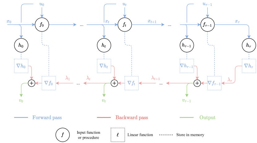
Figure 3: Computational scheme of a gradient oracle.

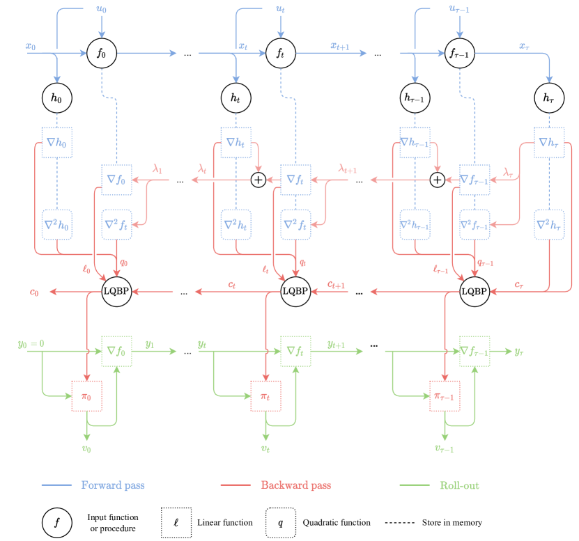
Figure 6: Computational scheme of a Newton oracle.

Gradient, Gauss-Newton, and Newton oracles are implemented by, respectively, Algo. 12, Algo. 13, Algo. 14. Additional line-searches are presented in Sec. 6. The computational scheme of a gradient oracle, i.e., gradient back-propagation, is illustrated in Fig. 3. The computational scheme of the Gauss-Newton oracle is presented in Fig. 4. Finally, the computational scheme of a Newton oracle is illustrated in Fig. 6.

Gradient back-propagation

For a gradient oracle (13), the procedure $\operatorname{LQBP}$ normally used to solve linear quadratic control problems simplifies to the procedure $\operatorname{LBP}$ presented in Algo. 3 that implements

$$\operatorname{LBP}:(\ell_{t}^{f},\ell_{t}^{h},c_{t+1},\nu)\rightarrow\left(\begin{array}[]{c}c_{t}:x\rightarrow\min_{u\in{\mathbb{R}}^{n_{u}}}\left\{\ell_{t}^{h}(x,u)+c_{t+1}(\ell_{t}^{f}(x,u))+\frac{\nu}{2}\|u\|_{2}^{2}\right\}\\ \pi_{t}:x\rightarrow\operatorname*{arg\,min}_{u\in{\mathbb{R}}^{n_{u}}}\left\{\ell_{t}^{h}(x,u)+c_{t+1}(\ell_{t}^{f}(x,u))+\frac{\nu}{2}\|u\|_{2}^{2}\right\}\end{array}\right),$$ (26)

for linear functions $\ell_{t}^{f},\ell_{t}^{h},c_{t+1}$. Plugging into the overall dynamic programming procedure, Algo. 3, the linearizations of the dynamics and the costs, we get that the gradient oracle, Algo. 6, computes affine cost-to-go functions of the form $c_{t}(y_{t})=j_{t}^{\top}y_{t}+j^{0}_{t}$ with

$$j_{\tau}=\nabla h_{\tau}(x_{\tau}),\quad j_{t}=\nabla_{x_{t}}h_{t}(x_{t},u_{t})+\nabla_{x_{t}}f_{t}(x_{t},u_{t})j_{t+1}\quad\mbox{for}\ t\in\{0,\ldots,\tau-1\}.$$

Moreover, the policies are independent of the state variables, i.e., $\pi_{t}(y_{t})=k_{t}$, with

$$k_{t}=-\nu^{-1}(\nabla_{u_{t}}h_{t}(x_{t},u_{t})+\nabla_{u_{t}}f_{t}(x_{t},u_{t})j_{t+1})=-\nu^{-1}\nabla_{u_{t}}(h\circ{g})({\bm{u}}).$$

The roll-out of these policies is independent of the dynamics and output directly the gradient up to a factor $-\nu^{-1}$. Note that we naturally retrieve the gradient back-propagation algorithm (Griewank and Walther,, 2008).

Simplifications

Some simplifications can be done in the implementations of the oracles. The gradient oracle can directly return the values of the gradient without the need for a roll-out phase. For the Gauss-Newton oracle, if there is no intermediate cost ($h_{t}=0$ for $t\in\{0,\ldots,\tau-1\}$), the oracle can be computed by solving the dual subproblem by making calls to an automatic differentiation procedure as done by, e.g., Roulet et al., (2019). For the Newton oracle, the quadratic approximations of the dynamics do not need to be stored and can simply be computed in the backward pass by computing the second derivative of $f_{t}^{\top}\lambda_{t+1}$ on $x_{t},u_{t}$ as explained in Sec. 7.

5 Differential Dynamic Programming Oracles

The original differential dynamic programming algorithm was developed by Jacobson and Mayne, (1970) and revisited by, e.g., Mayne and Polak, (1975); Murray and Yakowitz, (1984); Liao and Shoemaker, (1992); Tassa et al., (2014). The reader can verify from the aforementioned citations that our presentation matches the original formulation in, e.g., the quadratic case, while offering a larger perspective on the method that incorporates, e.g., linear quadratic approximations.

5.1 Derivation

5.1.1 Rationale

Denoting $h$ the total cost as in (8) and ${f^{[\tau]}}$ the control in $\tau$ dynamics $(f_{t})_{t=0}^{\tau-1}$, Differential Dynamic Programming (DDP) oracles consist in solving approximately

$$\min_{\bm{v}\in{\mathbb{R}}^{\tau{n_{u}}}}h({f^{[\tau]}}(\bar{x}_{0},{\bm{u}}+\bm{v}),{\bm{u}}+\bm{v}),$$

by means of a dynamic programming procedure and using the resulting policies to update the current sequence of controllers. For a consistent presentation with the classical optimization oracles presented in Sec. 4, we consider a regularized formulation of the DDP oracles, that is,

$$\min_{\bm{v}\in{\mathbb{R}}^{\tau{n_{u}}}}h({f^{[\tau]}}(\bar{x}_{0},{\bm{u}}+\bm{v}),{\bm{u}}+\bm{v})+\frac{\nu}{2}\|\bm{v}\|_{2}^{2},$$ (27)

for some regularization $\nu\geq 0$.

The objective in problem (27) can be rewritten as

$$h({f^{[\tau]}}(\bar{x}_{0},{\bm{u}}+\bm{v}),{\bm{u}}+\bm{v})=h({f^{[\tau]}}(\bar{x}_{0},{\bm{u}}))+\delta_{h}^{{f^{[\tau]}}(\bar{x}_{0},{\bm{u}})}(\delta_{f^{[\tau]}}^{\bar{x}_{0},{\bm{u}}}(0,\bm{v}),\bm{v}),$$ (28)

where for a function $f$, $\delta_{f}^{x}$ is the finite difference expression of $f$ around $x$ as defined in the notations in Eq. (2). In particular, $\delta_{f^{[\tau]}}^{\bar{x}_{0},{\bm{u}}}(0,\bm{v})$ is the trajectory defined by the finite differences of the dynamics given as

$$\delta_{f_{t}}^{x_{t},u_{t}}(y_{t},v_{t})=f_{t}(x_{t}+y_{t},u_{t}+v_{t})-f_{t}(x_{t},u_{t}).$$

The dynamic programming approach is then applied on the above dynamics. Namely, the goal is to solve

$$\min_{\begin{subarray}{c}v_{0},\ldots,v_{\tau-1}\in{\mathbb{R}}^{{n_{u}}}\\ y_{0},\ldots,y_{\tau}\in{\mathbb{R}}^{{n_{x}}}\end{subarray}} \sum_{t=0}^{\tau-1}\delta_{h_{t}}^{x_{t},u_{t}}(y_{t},v_{t})+\frac{\nu}{2}\|v_{t}\|_{2}^{2}+\delta_{h_{\tau}}^{x_{\tau}}(y_{\tau})$$ (29)

subject to $$y_{t+1}=\delta_{f_{t}}^{x_{t},u_{t}}(y_{t},v_{t})\quad\mbox{for}\ t\in\{0,\ldots,\tau-1\},\quad y_{0}=0,$$

by dynamic programming. Denote then $c_{t}^{*}$ the cost-to-go functions associated to problem (29) for $t\in\{0,\ldots\tau\}$. These cost-to-go functions satisfy the recursive equation

$$c_{t}^{*}(y_{t})=\min_{v_{t}\in{\mathbb{R}}^{n_{u}}}\left\{\delta_{h_{t}}^{x_{t},u_{t}}(y_{t},v_{t})+\frac{\nu}{2}\|v_{t}\|_{2}^{2}+c_{t+1}^{*}(\delta_{f_{t}}^{x_{t},u_{t}}(y_{t},v_{t}))\right\},$$ (30)

starting from $c_{\tau}^{*}=\delta_{h_{\tau}}^{x_{\tau}}$ and such that our objective is to compute $c_{0}^{*}(0)$. Since the dynamics $\delta_{f_{t}}^{x_{t},u_{t}}$ are not linear and the costs $\delta_{h_{t}}^{x_{t},u_{t}}$ are not quadratic, there is no analytical solution for the subproblem (30). To circumvent this issue, the cost-to-go functions are approximated as $c_{t}^{*}(y_{t})\approx c_{t}(y_{t}),$ where $c_{t}$ is computed from approximations of the dynamics and the costs. The approximation is done around the nominal value of the subproblem (29) which is ${\bm{v}}=0$ and corresponds to ${\bm{y}}=0$ and no change of the original objective in (28).

Denoting $m_{f}$ an expansion of a function $f$ around the origin such that $f(x)\approx f(0)+m_{f}(x)$, the cost-to-go functions are computed with a procedure

$$\widehat{\operatorname{BP}}:\delta_{t}^{f},\delta_{t}^{h},c_{t+1}\rightarrow\left(\begin{array}[]{c}c_{t}:y\rightarrow\min_{v\in{\mathbb{R}}^{n_{u}}}\left\{(\delta_{t}^{h}{+}c_{t+1}{\circ}\delta_{t}^{f})(0,0)+m_{\delta_{t}^{h}}(y,v)+m_{c_{t+1}\circ\delta_{t}^{f}}(y,v)+\frac{\nu}{2}\|v\|_{2}^{2}\right\},\\ \pi_{t}:y\rightarrow\operatorname*{arg\,min}_{v\in{\mathbb{R}}^{n_{u}}}\left\{m_{\delta_{t}^{h}}(y,v)+m_{c_{t+1}\circ\delta_{t}^{f}}(y,v)+\frac{\nu}{2}\|v\|_{2}^{2}\right\}\end{array}\right),$$ (31)

applied to the finite differences $\delta_{f_{t}}^{x_{t},u_{t}}\rightarrow\delta_{t}^{f}$ and $\delta_{h_{t}}^{x_{t},u_{t}}\rightarrow\delta_{t}^{h}$. A DDP oracle computes then a sequence of policies by iterating in a backward pass, starting from $c_{\tau}=m_{\delta_{h_{\tau}}^{x_{\tau}}}$,

$$c_{t},\pi_{t}=\widehat{\operatorname{BP}}(\delta_{f_{t}}^{x_{t},u_{t}},\delta_{h_{t}}^{x_{t},u_{t}},c_{t+1})\quad\mbox{for}\ t\in\{\tau-1,\ldots,0\}.$$ (32)

Given a set of policies, an approximate solution is given by rolling out the policies along the dynamics defining problem (29), i.e., by computing $v_{0},\ldots,v_{\tau-1}$ as

$$v_{t}=\pi_{t}(y_{t}),\qquad y_{t+1}=\delta_{f_{t}}^{x_{t},u_{t}}(y_{t},v_{t})=f_{t}(x_{t}+y_{t},u_{t}+v_{t})-f_{t}(x_{t},u_{t})\qquad\mbox{for $t=0,\ldots,\tau-1$}.$$ (33)

The main difference with the classical optimization oracles relies a priori in the computation of the policies in (32) detailed below and in the roll-out pass that uses the finite differences of the dynamics. Note that, while only the non-constant parts of the cost-to-go functions are useful to compute the policies, the overall procedure computes also the constant part of the cost-to-go functions. The latter is used for line-searches as detailed in Sec. 6.

5.1.2 Detailed Derivations of the Backward Passes

Linear Approximation

If we consider a linear approximation for the composition of the cost-to-go function and the dynamics, we have

$$m_{c_{t+1}\circ\delta_{f_{t}}^{x,u}}=\ell_{c_{t+1}\circ\delta_{f}^{x,u}}=\ell_{c_{t+1}}^{\delta_{f}^{x,u}(0,0)}\circ\ell_{\delta_{f}^{x,u}}=\ell_{c_{t+1}}\circ\ell_{f}^{x,u},$$

where we denote simply $\ell_{f}=\ell_{f}^{0}$ the linear expansion of a function $f$ around the origin.

Plugging this model into (31) and using linear approximations of the costs, the recursion (32) amounts to computing, starting from $c_{\tau}=\ell_{\delta_{h_{\tau}}^{x_{\tau},u_{\tau}}}=\ell_{h_{\tau}}^{x_{\tau},u_{\tau}}$,

$$c_{t}(y) =\min_{v\in{\mathbb{R}}^{{n_{u}}}}\delta_{h_{t}}^{x_{t},u_{t}}(0,0)+\ell_{\delta_{h_{t}}^{x_{t},u_{t}}}(y,v)+c_{t+1}(\delta_{f_{t}}^{x_{t},u_{t}}(0,0))+\ell_{c_{t+1}}(\ell_{f_{t}}^{x_{t},u_{t}}(y,v))+\frac{\nu}{2}\|v\|_{2}^{2},$$

$$=\min_{v\in{\mathbb{R}}^{{n_{u}}}}\ell_{h_{t}}^{x_{t},u_{t}}(y,v)+c_{t+1}(\ell_{f_{t}}^{x_{t},u_{t}}(y,v))+\frac{\nu}{2}\|v\|_{2}^{2},$$

where in the last line we used that the cost-to-go functions $c_{t}$ are necessarily affine, s.t. $c_{t+1}(y)=c_{t+1}(0)+\ell_{c_{t+1}}(y)$. We retrieve then the same recursion as the one used for a gradient oracle and the output policies are then the same. Since the computed policies are constant, they are not affected by the dynamics along which a roll-out phase is performed. In other words, the oracle returned by using linear approximations in a DDP approach is just a gradient oracle.

Linear Quadratic Approximation

If we consider a linear quadratic approximation for the composition of the cost-to-go function and the dynamics, we have

$$m_{c_{t+1}\circ\delta_{f^{x,u}}}=q_{c_{t+1}}^{\delta_{f}^{x,u}(0,0)}\circ\ell_{\delta_{f}^{x,u}}=q_{c_{t+1}}\circ\ell_{f}^{x,u},$$

where we denote simply $q_{f}=q_{f}^{0}$ the quadratic expansion of a function $f$ around the origin. Plugging this model into (31) and using quadratic approximations of the costs, the recursion (32) amounts to computing, starting from $c_{\tau}=q_{\delta_{h_{\tau}}^{x_{\tau},u_{\tau}}}=q_{h_{\tau}}^{x_{\tau},u_{\tau}}$,

$$c_{t}(y) =\min_{v\in{\mathbb{R}}^{{n_{u}}}}\delta_{h_{t}}^{x_{t},u_{t}}(0,0)+q_{\delta_{h_{t}}^{x_{t},u_{t}}}(y,v)+c_{t+1}(\delta_{f_{t}}^{x_{t},u_{t}}(0,0))+q_{c_{t+1}}^{\delta_{f}^{x,u}(0,0)}\circ\ell_{\delta_{f}^{x,u}}^{(0,0)}(y,v)+\frac{\nu}{2}\|v\|_{2}^{2}$$

$$=\min_{v\in{\mathbb{R}}^{{n_{u}}}}q_{h_{t}}^{x_{t},u_{t}}(y,v)+c_{t+1}(0)+q_{c_{t+1}}(\ell_{f_{t}}^{x_{t},u_{t}}(y,v))+\frac{\nu}{2}\|v\|_{2}^{2}.$$ (34)

If the costs $h_{t}$ are convex for all $t$ and $q_{h_{t}}^{x_{t},u_{t}}(y,\cdot)+\frac{\nu}{2}\|\cdot\|_{2}^{2}$ is strongly convex for all $t$ and all $y$, then the cost-to-go functions $c_{t}$ are convex quadratics for all $t$, i.e., $c_{t+1}(y)=c_{t+1}(0)+q_{c_{t+1}}(y)$. In that case, the recursion (34) simplifies as

$$c_{t}(y)=\min_{v\in{\mathbb{R}}^{{n_{u}}}}q_{h_{t}}^{x_{t},u_{t}}(y,v)+c_{t+1}(\ell_{f_{t}}^{x_{t},u_{t}}(y,v))+\frac{\nu}{2}\|v\|_{2}^{2},$$ (35)

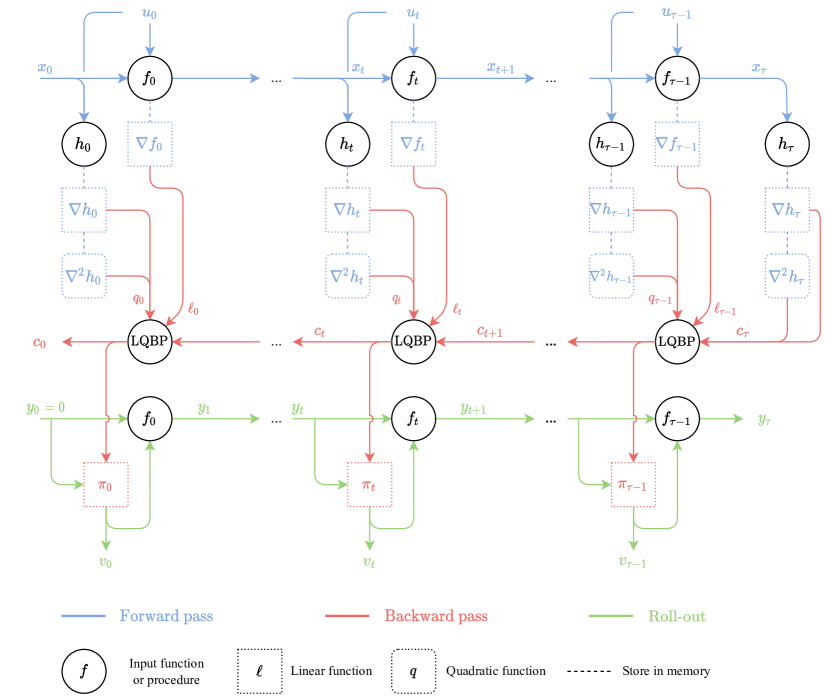
Figure 5: Computational scheme of a DDP oracle with linear quadratic approximations.

and the policies are given by the minimizer of Eq. (35). The recursion (35) is then the same as the recursion done when computing a Gauss-Newton oracle. Namely, the backward pass in this case is the backward pass of a Gauss-Newton oracle. Though the output policies are the same, the output of the oracle will differ since the roll-out phase does not follow the linearized trajectories in the DDP approach. The computational scheme of a DDP approach with linear quadratic approximations presented in Fig. 5 is then almost the same as the one of a Gauss-Newton oracle presented in Fig. 4, except that in the roll-out phase the linear approximations of the dynamics are replaced by finite differences of the dynamics.

Quadratic Approximation

If we consider a quadratic approximation for the composition of the cost-to-go function and the dynamics, we get

$$m_{c_{t+1}\circ\delta_{f}^{x,u}}=q_{c_{t+1}\circ\delta_{f}^{x,u}}=\frac{1}{2}\nabla^{2}f(x,u)[\cdot,\cdot,\nabla c_{t+1}(0)]+q_{c_{t+1}}\circ\ell_{f}^{x,u},$$

where $\nabla^{2}f(x,u)[\cdot,\cdot,\lambda]$ is defined in (18). Plugging this model into (31) and using quadratic approximations of the costs, the recursion (32) amounts to, starting from $c_{\tau}=q_{\delta_{h_{\tau}}^{x_{\tau},u_{\tau}}}=q_{h_{\tau}}^{x_{\tau},u_{\tau}}$,

$$c_{t}(y) =\min_{v\in{\mathbb{R}}^{{n_{u}}}}\delta_{h_{t}}^{x_{t},u_{t}}(0,0)+q_{\delta_{h_{t}}^{x_{t},u_{t}}}(y,v)+c_{t+1}(\delta_{f_{t}}^{x_{t},u_{t}}(0,0))+q_{c_{t+1}\circ\delta_{f_{t}}^{x,u}}(y,v)+\frac{\nu}{2}\|v\|_{2}^{2}$$ (36)

$$=\min_{v\in{\mathbb{R}}^{{n_{u}}}}q_{h_{t}}^{x_{t},u_{t}}(y,v)+c_{t+1}(0)+q_{c_{t+1}}\circ\ell_{f_{t}}^{x_{t},u_{t}}(y,v)+\frac{1}{2}\nabla^{2}f_{t}(x_{t},u_{t})[\cdot,\cdot,\nabla c_{t+1}(0)](y,v)+\frac{\nu}{2}\|v\|_{2}^{2}.$$

Provided that the costs are convex and that $q_{h_{t}}^{x_{t},u_{t}}(y,\cdot)+\frac{1}{2}\nabla^{2}f_{t}(x_{t},u_{t})[\cdot,\cdot,\nabla c_{t+1}(0)](y,\cdot)+\frac{\nu}{2}\|\cdot\|_{2}^{2}$ is strongly convex for all $t$ and all $y$, the cost-to-go functions $c_{t}$ are convex quadratics for all $t$. In that case, the recursion (36) simplifies as

$$c_{t}(y)=\min_{v\in{\mathbb{R}}^{{n_{u}}}}q_{h_{t}}^{x_{t},u_{t}}(y,v)+c_{t+1}(\ell_{f_{t}}^{x_{t},u_{t}}(y,v))+\frac{1}{2}\nabla^{2}f_{t}(x_{t},u_{t})[\cdot,\cdot,\nabla c_{t+1}(0)](y,v)+\frac{\nu}{2}\|v\|_{2}^{2},$$ (37)

and the policies are given by the minimizer of Eq. (37). The overall backward pass is detailed in Algo. 9.

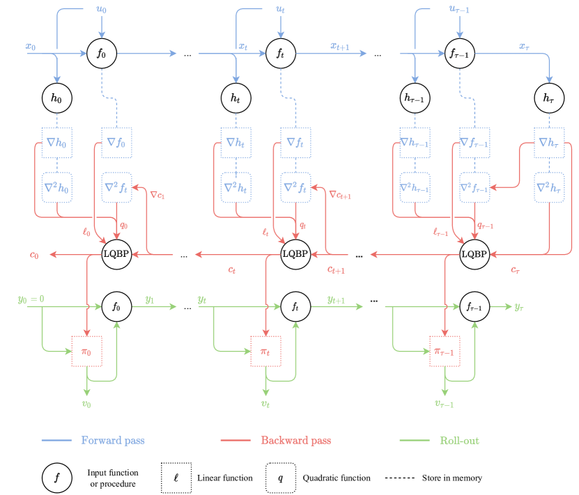
Figure 7: Computational scheme of a DDP oracle with quadratic approximations.

Compared to the backward pass of the Newton oracle in Algo. 8, we note that the additional cost derived from the curvatures of the dynamics is not computed the same way. Namely, the Newton oracle computes this additional cost by using back-propagated adjoint variables in Eq. (17), while in the DDP approach the additional cost is directly defined through the previously computed cost-to-go function. Fig. 7 illustrates the computational scheme of the implementation of DDP with quadratic approximations and can be compared to the computational scheme of the Newton oracle in Fig. 6.

Note that, while we used second order Taylor expansions for the compositions and the costs, the approximate cost-to-go-functions $c_{t}$ are not second order Taylor expansion of the true cost-to-go functions $c_{t}^{*}$, except for $c_{\tau}$. Indeed, $c_{t}$ is computed as an approximate solution of the Bellman equation. The true Taylor expansion of the cost-to-go function requires the gradient and the Hessian of the cost and the dynamic in Eq. (36) computed at the minimizer of the subproblem. Here, since we only use an approximation of the minimizer, we do not have access to the true gradient and Hessian of the cost-to-go function.

5.2 Implementation

The implementation of the DDP oracles follows the same steps as the ones given for classical optimization oracles as detailed below. The implementation of a DDP oracle with linear quadratic approximations is given in Algo. 15 and illustrated in Fig. 5. The implementation of a DDP oracle with quadratic approximations is given in Algo. 16 and illustrated in Fig. 7.

1. Forward pass: As for the classical optimization methods, the forward pass is provided in Algo. 5 which gathers the information necessary for the backward pass. Namely, the oracle starts with Algo. 5 and computes

   $$\mathcal{J}({\bm{u}}),(m_{f_{t}}^{x_{t},u_{t}})_{t=0}^{\tau-1},(m_{h_{t}}^{x_{t},u_{t}})_{t=0}^{\tau-1},m_{h_{\tau}}^{x_{\tau}}=\operatorname{Forward}({\bm{u}},(f_{t})_{t=0}^{\tau-1},(h_{t})_{t=0}^{\tau},\bar{x}_{0},o_{f},o_{h}),$$

   where $o_{f}$ and $o_{h}$ define the order of approximations used for the dynamics and the costs respectively.

2. Backward pass: As for the classical optimization oracles, the backward pass can generally be written

   $$(\pi_{t})_{t=0}^{\tau-1},c_{0}=\operatorname{Backward}((m_{f_{t}}^{x_{t},u_{t}})_{t=0}^{\tau-1},(m_{h_{t}}^{x_{t},u_{t}})_{t=0}^{\tau-1},m_{h_{\tau}}^{x_{\tau}},\nu),$$

   If linear approximations are used, the backward pass is given in Algo. 6, if linear quadratic approximations are used, the backward pass is given in Algo. 7 and if quadratic approximations are used, the backward pass is given in Algo. 9.

3. Roll-out pass: The roll-out phase differs by using finite differences of the original dynamics of problem (29) rather than the linearized dynamics. Formally, given a sequence of policies $(\pi_{t})_{t=0}^{\tau-1}$, the oracles are then given as $\bm{v}=(v_{0};\ldots;v_{\tau-1})$ computed, for $y_{0}=0$, by Algo. 11 as

   $$\bm{v}=\operatorname{Roll}(y_{0},(\pi_{t})_{t=0}^{\tau-1},(\delta_{f_{t}}^{x_{t},u_{t}})_{t=0}^{\tau-1}),$$

   where $\delta_{f_{t}}^{x_{t},u_{t}}(y_{t},v_{t})=f_{t}(x_{t}+y_{t},u_{t}+v_{t})-f_{t}(x_{t},u_{t})$.

6 Line-searches

So far, we defined procedures that, given a command and some regularization parameter, output a direction that minimizes an approximation of the objective or approximately minimizes a shifted objective. Given access to such procedures, the next command can be computed in several ways. The main criterion is to ensure that the value of the objective decreases along the iterations, which is generally done by a line-search.

In the following, we only consider oracles based on linear quadratic or quadratic approximations of the objective such as Gauss-Newton and Newton, and refer the reader to Nocedal and Wright, (2006) for classical line-searches for gradient descent.

6.1 Rules

We start by considering the implementation of line-searches for classical optimization oracles which can again exploit the dynamical structure of the problem and are mimicked by differential dynamic programming approaches. We consider, as in Sec. 4, that we have access to an oracle for an objective $\mathcal{J}$, that, given a command ${\bm{u}}\in{\mathbb{R}}^{\tau{n_{u}}}$ and any regularization $\nu\geq 0$, outputs

$$\operatorname{Oracle}_{\nu}(\mathcal{J})({\bm{u}})=\operatorname*{arg\,min}_{\bm{v}\in{\mathbb{R}}^{\tau{n_{u}}}}m_{\mathcal{J}}^{\bm{u}}(\bm{v})+\frac{\nu}{2}\|\bm{v}\|_{2}^{2},$$ (38)

where $m_{\mathcal{J}}^{\bm{u}}$ is a linear quadratic or quadratic expansion of the objective $\mathcal{J}$ around ${\bm{u}}$ s.t. $\mathcal{J}({\bm{u}}+\bm{v})\approx\mathcal{J}({\bm{u}})+m_{\mathcal{J}}^{\bm{u}}(\bm{v})$. Given such an oracle, we can define a new candidate command that decreases the value of the objective in several ways.

6.1.1 Directional Steps

The next iterate can be defined along the direction provided by the oracle, as long as this direction is a descent direction. Namely, the next iterate can be computed as

$${\bm{u}}^{{\operatorname{next}}}={\bm{u}}+\gamma\bm{v},\quad\mbox{with}\ \bm{v}=\operatorname{Oracle}_{\nu}(\mathcal{J})({\bm{u}})\ \mbox{for}\ \nu\geq 0\ \mbox{s.t.}\ \nabla\mathcal{J}({\bm{u}})^{\top}\bm{v}<0,$$ (39)

where the stepsize $\gamma$ is chosen to satisfy, e.g., an Armijo condition, that is,

$$\mathcal{J}({\bm{u}}+\gamma\bm{v})\leq\mathcal{J}({\bm{u}})+\frac{\gamma}{2}\nabla\mathcal{J}({\bm{u}})^{\top}\bm{v}.$$ (40)

In this case, the search is usually initialized at each step with $\gamma=1$. If condition (40) is not satisfied for $\gamma=1$, the stepsize is decreased by a factor $\rho_{\operatorname{dec}}<1$ until condition (40) is satisfied. If a stepsize $\gamma=1$ is accepted, then the linear quadratic or quadratic algorithms may exhibit a quadratic local convergence (Nocedal and Wright,, 2006). Alternative line-search criterions such as Wolfe’s condition or trust-region methods can also be implemented (Nocedal and Wright,, 2006).

6.1.2 Regularized Steps

Given a current iterate ${\bm{u}}\in{\mathbb{R}}^{\tau{n_{u}}}$, we can find a regularization such that the current iterate plus the direction output by the oracle decreases the objective. Namely, the next command can be computed as

$${\bm{u}}^{{\operatorname{next}}}={\bm{u}}+\bm{v}^{\gamma},\quad\mbox{where}\quad\bm{v}^{\gamma}=\operatorname{Oracle}_{1/\gamma}(\mathcal{J})({\bm{u}})=\operatorname*{arg\,min}_{\bm{v}\in{\mathbb{R}}^{\tau{n_{u}}}}m_{\mathcal{J}}^{\bm{u}}(\bm{v})+\frac{1}{2\gamma}\|\bm{v}\|_{2}^{2},\qquad$$ (41)

where the parameter $\gamma>0$ acts as a stepsize that controls how large should be the step (the smaller the parameter $\gamma$, the smaller the step $\bm{v}^{\gamma}$). The stepsize $\gamma$ can then be chosen to satisfy

$$\mathcal{J}({\bm{u}}+\bm{v}^{\gamma})\leq\mathcal{J}({\bm{u}})+m_{\mathcal{J}}^{\bm{u}}(\bm{v}^{\gamma})+\frac{1}{2\gamma}\|\bm{v}^{\gamma}\|_{2}^{2},$$ (42)

which ensures a sufficient decrease of the objective to, e.g., prove convergence to stationary points (Roulet et al.,, 2019). In practice, as for the line-search on the descent direction, given an initial stepsize for the iteration, the stepsize is either selected or reduced by a factor $\rho_{\operatorname{dec}}$ until condition (42) is satisfied. However, here, we initialize the stepsize at each iteration as $\rho_{\operatorname{inc}}\gamma_{prev}$ where $\gamma_{prev}$ is the stepsize selected at the previous iteration and $\rho_{\operatorname{inc}}>1$ is an increasing factor. By trying a larger stepsize at each iteration, we may benefit from larger steps in some regions of the optimization path. Note that such an approach is akin to trust region methods which increase the radius of the trust region at each iteration depending on the success of each iteration (Nocedal and Wright,, 2006).

In practice, we observed that, when using regularized steps, acceptable stepsizes for condition (42) tend to be arbitrarily large as the iterations increase. Namely, we tried choosing $\rho_{\operatorname{inc}}=10$ and observed that the acceptable stepsizes tended to plus infinity with such a procedure. To better capture this tendency, we consider regularizations that may depend on the current state and of the form $\nu({\bm{u}})\propto\|\nabla h({\bm{x}},{\bm{u}})\|_{2}$, i.e., stepsizes of the form $\gamma({\bm{u}})=\bar{\gamma}/\|\nabla h({\bm{x}},{\bm{u}})\|_{2}$. The line-search is then performed on $\bar{\gamma}$ only. Intuitively, as we are getting closer to a stationary point, quadratic models are getting more accurate to describe the objective. By scaling the regularization with respect to $\|\nabla h({\bm{x}},{\bm{u}})\|_{2}$, which is a measure of stationarity, we may better capture such behavior. Note that for $\nu=0$, we retrieve the iteration with a descent direction of stepsize $\gamma=1$ described above.

6.2 Implementation

6.2.1 Directional Steps

The Armijo condition (40) can be computed directly from the knowledge of a gradient oracle and the chosen oracle (such as Gauss-Newton or Newton). We present here the implementation of the line-search in terms of the dynamical structure of the problem. Denote

$$(\pi_{t})_{t=0}^{\tau-1},c_{0}=\operatorname{Backward}((m_{f_{t}}^{x_{t},u_{t}})_{t=0}^{\tau-1},(m_{h_{t}}^{x_{t},u_{t}})_{t=0}^{\tau-1},m_{h_{\tau}}^{x_{\tau}},\nu)$$

the policies and the value of the cost-to-go function output by the backward pass of the considered oracle, i.e., Gauss-Newton or Newton.

By definition, $c_{0}(0)$ is the minimum of the corresponding linear quadratic control problem (16). Moreover, the linear quadratic control problem can be summarized as a quadratic problem of the form $\min_{\bm{v}}m_{\mathcal{J}}(\bm{v})+\frac{\nu}{2}\|\bm{v}\|_{2}^{2}=\min_{\bm{v}}\frac{1}{2}\bm{v}^{\top}(Q+\nu\operatorname{I})\bm{v}+\nabla\mathcal{J}({\bm{u}})^{\top}\bm{v}$ with $Q$ a quadratic that is either the Hessian of $\mathcal{J}$ for a Newton oracle or an approximation of it for a Gauss-Newton oracle. Therefore, we have that, for a Newton or a Gauss-Newton oracle $\bm{v}=\operatorname{Oracle}_{1/\gamma}(\mathcal{J})$,

$$\frac{1}{2}\nabla\mathcal{J}({\bm{u}})^{\top}\bm{v}=-\frac{1}{2}\nabla\mathcal{J}({\bm{u}})^{\top}(Q+\nu\operatorname{I})^{-1}\nabla\mathcal{J}({\bm{u}})=\min_{\bm{v}\in{\mathbb{R}}^{\tau{n_{u}}}}m_{\mathcal{J}}(\bm{v})+\frac{\nu}{2}\|\bm{v}\|_{2}^{2}=c_{0}(0).$$

Therefore the right-hand part of condition (40) can be given by the value of the cost-to-go function $c_{0}(0)$. On the other hand, sequences of controllers of the form $\gamma\bm{v}$ can be defined by modifying the policies output in the backward pass as shown in the following lemma adapted from Liao and Shoemaker, (1992, Theorem 1).

Lemma 6.1.

Given a sequence of affine policies $(\pi_{t})_{t=0}^{\tau-1}$, linear dynamics $(\ell_{t})_{t=0}^{\tau-1}$ and an initial state $y_{0}=0$, denote $\bm{v}^{*}=\operatorname{Roll}(y_{0},(\pi_{t})_{t=0}^{\tau-1},(\ell_{t})_{t=0}^{\tau-1})$ and $\pi_{t}^{\gamma}:y\rightarrow\gamma\pi_{t}(0)+\nabla\pi_{t}(0)^{\top}y$ for $t=0,\ldots,\tau-1$. We have that

$$\gamma\bm{v}^{*} =\bm{v}^{\gamma},\quad\mbox{where}\quad\bm{v}^{\gamma}=\operatorname{Roll}(y_{0},(\pi_{t}^{\gamma})_{t=0}^{\tau-1},(\ell_{t})_{t=0}^{\tau-1}).$$

Proof.

Define $(y_{t}^{\gamma})_{t=0}^{\tau-1}$ as $y_{t+1}^{\gamma}=\ell_{t}(y_{t}^{\gamma},\pi_{t}(y_{t}^{\gamma}))$ for $t\in\{0,\ldots,\tau-1\}$ with $y^{\gamma}_{0}=0$. We have that $y^{\gamma}_{1}$ is linear w.r.t. $\gamma$. Proceeding by induction, we have that $y_{t}^{\gamma}$ is linear w.r.t. $\gamma$ using the form of $\pi_{t}^{\gamma}$ and the fact that $\ell_{t}$ is linear. Therefore $v_{t}^{\gamma}=\pi_{t}^{\gamma}(y_{t}^{\gamma})$ is linear w.r.t. $\gamma$ which gives the claim. ∎

Therefore, computing the next sequence of controllers by moving along a descent direction as in (39) according to an Armijo condition (40) amounts to computing, with Algo. 17,

$${\bm{u}}^{{\operatorname{next}}} =\operatorname{LineSearch}({\bm{u}},(h_{t})_{t=0}^{\tau},(f_{t})_{t=0}^{\tau-1},(\ell_{f_{t}}^{x_{t},u_{t}})_{t=0}^{\tau-1},\operatorname{Pol}),$$

where $$\operatorname{Pol}:\gamma\rightarrow\left(\begin{array}[]{ll}(\pi_{t}^{\gamma}:&y\rightarrow\gamma\pi_{t}(0)+\nabla\pi_{t}(0)^{\top}y)_{t=0}^{\tau-1}\\ \hskip 6.0ptc_{0}^{\gamma}:&y\rightarrow\gamma c_{0}(y)\end{array}\right)$$

$$(\pi_{t})_{t=0}^{\tau-1},c_{0}=\operatorname{Backward}((m_{f_{t}}^{x_{t},u_{t}})_{t=0}^{\tau-1},(m_{h_{t}}^{x_{t},u_{t}})_{t=0}^{\tau-1},m_{h_{\tau}}^{x_{\tau}},\nu),\ \mbox{for}\ \nu\geq 0\ \mbox{s.t.}\ c_{0}(0)<0,$$

where $\operatorname{Backward}\in\{\operatorname{Backward}_{\operatorname{GN}},\operatorname{Backward}_{\operatorname{NE}}\}$ is given in Algo. 7 or Algo. 8.

In practice, in our implementation of the backward passes in Algo. 7, Algo. 8, the returned initial cost-to-go function is either negative if the step is well defined or infinite if it is not. To find a regularization that ensures a descent direction, i.e., $c_{0}(0)<0$, it suffices thus to find a feasible step. In our implementation, we first try to compute a descent direction without regularization ($\nu=0$), then try a small regularization $\nu=10^{-6}$, which we increase by 10 until a finite negative cost-to-go function $c_{0}(0)$ is returned. See Algo. 18 for an instance of such implementation.

From the above discussion, it is clear that one iteration of the Iterative Linear Quadratic Regulator algorithm described in Sec. 2.3 uses a Gauss-Newton oracle without regularization to move along the direction of the oracle by using an Armijo condition. The overall iteration is given in Algo. 18, where we added a procedure to ensure that the output direction is a descent direction. All other algorithms, with or without regularization can be written in a similar way using a forward, a backward pass, and multiple roll-out phases until the next sequence of controllers is found.

6.2.2 Regularized Steps

For regularized steps, the line-search (42) requires computing $m_{\mathcal{J}}^{\bm{u}}(v^{\gamma})+\frac{1}{2\gamma}\|v^{\gamma}\|_{2}^{2}$. This is by definition the minimum of the sub-problem that is computed by dynamic programming. This minimum can therefore be accessed as $m_{\mathcal{J}}^{\bm{u}}(\bm{v}^{\gamma})+\frac{1}{2\gamma}\|\bm{v}^{\gamma}\|_{2}^{2}=c_{0}(0)$ for $c_{0}$ output by the backward pass with a regularization $\nu=1/\gamma$. Overall, the next sequence of controls is then provided through the line-search procedure given in Algo. 17 as

$${\bm{u}}^{{\operatorname{next}}} =\operatorname{LineSearch}({\bm{u}},(h_{t})_{t=0}^{\tau},(f_{t})_{t=0}^{\tau-1},(\ell_{f_{t}}^{x_{t},u_{t}})_{t=0}^{\tau-1},\operatorname{Pol}),$$

where $$\operatorname{Pol}:\gamma\rightarrow\operatorname{Backward}((m_{f_{t}}^{x_{t},u_{t}})_{t=0}^{\tau-1},(m_{h_{t}}^{x_{t},u_{t}})_{t=0}^{\tau-1},m_{h_{\tau}}^{x_{\tau}},1/\gamma),$$

where $\operatorname{Backward}\in\{\operatorname{Backward}_{\operatorname{GN}},\operatorname{Backward}_{\operatorname{NE}}\}$ is given in Algo. 7 or Algo. 8.

6.2.3 Line-searches for Differential Dynamic Programming Approaches

The line-search for DDP approaches as presented by, e.g., Liao and Shoemaker, (1992, Sec. 2.2) based on Jacobson and Mayne, (1970), mimics the one done for the classical optimization oracles except that the policies are rolled out on the original dynamics. Namely, the usual line-search consists in applying Algo. 17 as follows

$${\bm{u}}^{{\operatorname{next}}} =\operatorname{LineSearch}({\bm{u}},(h_{t})_{t=0}^{\tau},(f_{t})_{t=0}^{\tau-1},(\delta_{f_{t}}^{x_{t},u_{t}})_{t=0}^{\tau-1},\operatorname{Pol})$$

where $$\operatorname{Pol}:\gamma\rightarrow\left(\begin{array}[]{ll}(\pi_{t}^{\gamma}:&y\rightarrow\gamma\pi_{t}(0)+\nabla\pi_{t}(0)^{\top}y)_{t=0}^{\tau-1},\\ \hskip 6.0ptc_{0}^{\gamma}:&y\rightarrow\gamma c_{0}(y)\end{array}\right)$$

$$(\pi_{t})_{t=0}^{\tau-1},c_{0}=\operatorname{Backward}((m_{f_{t}}^{x_{t},u_{t}})_{t=0}^{\tau-1},(m_{h_{t}}^{x_{t},u_{t}})_{t=0}^{\tau-1},m_{h_{\tau}}^{x_{\tau}},\nu)\ \mbox{for}\ \nu\geq 0\ \mbox{s.t.}\ c_{0}(0)<0,$$

where $\operatorname{Backward}\in\{\operatorname{Backward}_{\operatorname{GN}},\operatorname{Backward}_{\operatorname{DDP}}\}$ is given by Algo. 7 or Algo. 9. As for the classical optimization oracles, a direction is first computed without regularization and if the resulting direction is not a descent direction a small regularization is added to ensure that $c_{0}(0)<0$.

We also consider line-searches based on selecting an appropriate regularization. Namely, we consider line-searches of the form

$${\bm{u}}^{{\operatorname{next}}} =\operatorname{LineSearch}({\bm{u}},(h_{t})_{t=0}^{\tau},(f_{t})_{t=0}^{\tau-1},(\delta_{f_{t}}^{x_{t},u_{t}})_{t=0}^{\tau-1},\operatorname{Pol}),$$

where $$\operatorname{Pol}:\gamma\rightarrow\operatorname{Backward}((m_{f_{t}}^{x_{t},u_{t}})_{t=0}^{\tau-1},(m_{h_{t}}^{x_{t},u_{t}})_{t=0}^{\tau-1},m_{h_{\tau}}^{x_{\tau}},1/\gamma),$$

where $\operatorname{Backward}\in\{\operatorname{Backward}_{\operatorname{GN}},\operatorname{Backward}_{\operatorname{DDP}}\}$ is given by Algo. 7 or Algo. 9.

7 Computational Complexities

7.1 Formal Computational Complexities

We present in Table 1 the computational complexities of the algorithms following the implementations described in Sec. 4 and Sec. 5 and detailed in Sec. 9. We ignore the additional cost of the line-searches which requires a theoretical analysis of the admissible stepsizes depending on the smoothness properties of the dynamics and the costs. We consider for simplicity that the cost of evaluating a function $f:{\mathbb{R}}^{d}\rightarrow{\mathbb{R}}^{n}$ is of the order of $O(nd)$, as it is the case if $f$ is linear. For the computational complexities of the core operation of the backward pass, i.e, $\operatorname{LQBP}$ in Algo. 2 or $\operatorname{LBP}$ in Algo. 3, we simply give the leading computational complexities, which, in the case of $\operatorname{LQBP}$, are the matrix multiplications and inversions.

The time complexities differ depending on whether linear or quadratic approximations of the costs are used. In the latter case, matrices of size ${n_{u}}\times{n_{u}}$ need to be inverted and matrices of size ${n_{x}}\times{n_{x}}$ need to be multiplied. However, all oracles have a linear time complexity with respect to the horizon $\tau$.

We note that the space complexities of the gradient descent and the Gauss-Newton method or the DDP approach with linear quadratic approximations are essentially the same. On the other hand, the space complexity of the Newton oracle is a priori larger.

7.2 Computational Complexities in a Differentiable Programming Framework

The decomposition of each oracle between forward, backward and roll-out passes has the advantage to clarify the discrepancies between each approach. However, storing the linear or quadratic approximations of the costs or the dynamics may come at a prohibitive cost in terms of memory. A careful implementation of these oracles only requires storing in memory the function and the inputs given at each time-step. Namely, the forward pass can simply keep in memory $h_{t},f_{t},x_{t},u_{t}$ for $t\in\{0,\ldots,\tau\}$. The backward pass computes then, on the fly, the information necessary to compute the policies.

The previous time complexities of the forward pass, corresponding to the computations of the gradients of the dynamics or the costs and Hessians of the costs, are then incurred during the backward pass. A major difference lies in the computation of the quadratic information of the dynamic required in quadratic oracles such as a Newton oracle or a DDP oracle with quadratic approximations. Indeed, a closer look at Algo. 8 and Algo. 9 show that only the Hessians of scalar functions of the form $x,u\rightarrow f(x,u)^{\top}\lambda$ need to be computed, which comes at a cost $({n_{x}}+{n_{u}})^{2}$. In comparison, the cost of computing the second order information of $f$ is $O(({n_{x}}+{n_{u}})^{2}{n_{x}})$. As an example, Algo. 10 presents an implementation of a Newton step using stored functions and inputs.

The computational complexities of the oracles when the dynamics and the costs functions are stored in memory are presented in Table 2. We consider for simplicity that the memory cost of storing the information necessary to evaluate a function $f:{\mathbb{R}}^{d}\rightarrow{\mathbb{R}}^{n}$ is $nd$ as it is the case for a linear function $f$.

In summary, by considering an implementation that simply stores in memory the inputs and the programs that implement the functions, a Newton oracle and an oracle based on a DDP approach with quadratic approximation have the same time and space complexities as their linear quadratic counterparts up to constant factors. This remark was done by Nganga and Wensing, (2021) for implementing a DDP algorithm with quadratic approximations.

	Time complexities of the forward pass in Algo. 5
Function eval. ($o_{f}=o_{h}=0$)	$\tau\Big{(}\underbrace{{n_{x}}^{2}{+}{n_{x}}{n_{u}}}_{f_{t}}{+}\underbrace{{n_{x}}{+}{n_{u}}}_{h_{t}}\Big{)}{=}O(\tau({n_{x}}^{2}{+}{n_{x}}{n_{u}}))$
Linearization ($o_{f}=o_{h}=1$)	$\tau\Big{(}\underbrace{{n_{x}}^{2}{+}{n_{x}}{n_{u}}}_{f_{t},\nabla f_{t}}{+}\underbrace{{n_{x}}{+}{n_{u}}}_{h_{t},\nabla h_{t}}\Big{)}{=}O(\tau({n_{x}}^{2}{+}{n_{x}}{n_{u}}))$
Lin.-quad. ($o_{f}=1,o_{h}=2$)	$\tau\Big{(}\underbrace{{n_{x}}^{2}{+}{n_{x}}{n_{u}}}_{f_{t},\nabla f_{t}}{+}\underbrace{{n_{x}}{+}{n_{u}}}_{h_{t},\nabla h_{t}}{+}\underbrace{{n_{x}}^{2}{+}{n_{u}}^{2}{+}{n_{x}}{n_{u}}}_{\nabla^{2}h_{t}}\Big{)}{=}O(\tau({n_{x}}{+}{n_{u}})^{2})$
Quad. ($o_{f}=o_{h}=2$)	$\tau\Big{(}\underbrace{{n_{x}}^{2}{+}{n_{x}}{n_{u}}}_{f_{t},\nabla f_{t}}{+}\underbrace{({n_{x}}^{2}{+}{n_{u}}^{2}{+}{n_{x}}{n_{u}}){n_{x}}}_{\nabla^{2}f_{t}}{+}\underbrace{{n_{x}}{+}{n_{u}}}_{h_{t},\nabla h_{t}}{+}\underbrace{{n_{x}}^{2}{+}{n_{u}}^{2}{+}{n_{x}}{n_{u}}}_{\nabla^{2}h_{t}}\Big{)}{=}O(\tau{n_{x}}({n_{x}}{+}{n_{u}})^{2})$

	Space complexities of the forward pass in Algo. 5
Function eval. ($o_{f}=o_{h}=0$)	$0$
Linearization ($o_{f}=o_{h}=1$)	$\tau\Big{(}\underbrace{{n_{x}}^{2}{+}{n_{x}}{n_{u}}}_{\nabla f_{t}}{+}\underbrace{{n_{x}}{+}{n_{u}}}_{\nabla h_{t}}\Big{)}{=}O(\tau({n_{x}}^{2}{+}{n_{x}}{n_{u}}))$
Lin.-quad. ($o_{f}=1,o_{h}=2$)	$\tau\Big{(}\underbrace{{n_{x}}^{2}{+}{n_{x}}{n_{u}}}_{\nabla f_{t}}{+}\underbrace{{n_{x}}{+}{n_{u}}}_{\nabla h_{t}}{+}\underbrace{{n_{x}}^{2}{+}{n_{u}}^{2}{+}{n_{x}}{n_{u}}}_{\nabla^{2}h_{t}}\Big{)}{=}O(\tau({n_{x}}{+}{n_{u}})^{2})$
Quad. ($o_{f}=o_{h}=2$)	$\tau\Big{(}\underbrace{{n_{x}}^{2}{+}{n_{x}}{n_{u}}}_{\nabla f_{t}}{+}\underbrace{({n_{x}}^{2}{+}{n_{u}}^{2}{+}{n_{x}}{n_{u}}){n_{x}}}_{\nabla^{2}f_{t}}{+}\underbrace{{n_{x}}{+}{n_{u}}}_{\nabla h_{t}}{+}\underbrace{{n_{x}}^{2}{+}{n_{u}}^{2}{+}{n_{x}}{n_{u}}}_{\nabla^{2}h_{t}}\Big{)}{=}O(\tau{n_{x}}({n_{x}}{+}{n_{u}})^{2})$

	Time complexities of the backward passes in Algo. 6, 7, 8, 9 and the roll-out in Algo. 11
GD	$\tau\Big{(}\underbrace{{n_{x}}^{2}{+}{n_{x}}{n_{u}}}_{\textrm{Roll}}{+}\underbrace{{n_{x}}^{2}{+}{n_{x}}{n_{u}}}_{\operatorname{LBP}}\Big{)}{=}O(\tau({n_{x}}^{2}{+}{n_{x}}{n_{u}}))$
GN/DDP-LQ	$\tau\Big{(}\underbrace{{n_{x}}^{2}{+}{n_{x}}{n_{u}}}_{\textrm{Roll}}{+}\underbrace{{n_{x}}^{3}{+}{n_{u}}^{3}{+}{n_{u}}^{2}{n_{x}}}_{\operatorname{LQBP}}\Big{)}{=}O(\tau({n_{x}}{+}{n_{u}})^{3})$
NE/DDP-Q	$\tau\Big{(}\underbrace{{n_{x}}^{2}{+}{n_{x}}{n_{u}}}_{\textrm{Roll}}{+}\underbrace{{n_{x}}^{3}{+}{n_{u}}^{3}{+}{n_{u}}^{2}{n_{x}}}_{\operatorname{LQBP}}{+}\underbrace{({n_{x}}^{2}{+}{n_{u}}^{2}{+}{n_{x}}{n_{u}}){n_{x}}}_{\nabla f_{t}^{2}[\cdot,\cdot,\lambda]}\Big{)}{=}O(\tau({n_{x}}{+}{n_{u}})^{3})$

Table 1: Space and time complexities of the oracles of Sec. 4 and 5. GD stands for gradient Descent, GN for Gauss-Newton, NE for Newton, DDP-LQ and DDP-Q stand for DDP with linear quadratic or quadratic approx.

	Time complexities of the forward pass
All cases	$\tau\Big{(}\underbrace{{n_{x}}^{2}{+}{n_{x}}{n_{u}}}_{f_{t}}{+}\underbrace{{n_{x}}{+}{n_{u}}}_{h_{t}}\Big{)}{=}O(\tau({n_{x}}^{2}{+}{n_{x}}{n_{u}}))$

	Space complexities of the forward pass
Function eval.	$0$
All other cases	$\tau\Big{(}\underbrace{{n_{x}}^{2}{+}{n_{x}}{n_{u}}}_{f_{t}}{+}\underbrace{{n_{x}}{+}{n_{u}}}_{h_{t}}\Big{)}{=}O(\tau({n_{x}}^{2}{+}{n_{x}}{n_{u}}))$

	Time complexities of the backward passes
GD	$\tau\Big{(}\underbrace{{n_{x}}^{2}{+}{n_{x}}{n_{u}}}_{\nabla f_{t}}{+}\underbrace{{n_{x}}{+}{n_{u}}}_{\nabla h_{t}}{+}\underbrace{{n_{x}}^{2}{+}{n_{x}}{n_{u}}}_{\textrm{Roll}}{+}\underbrace{{n_{x}}^{2}{+}{n_{x}}{n_{u}}}_{\operatorname{LBP}}\Big{)}{=}O(\tau({n_{x}}^{2}{+}{n_{x}}{n_{u}}))$
GN/DDP-LQ	$\tau\Big{(}\underbrace{{n_{x}}^{2}{+}{n_{x}}{n_{u}}}_{\nabla f_{t}}{+}\underbrace{{n_{x}}{+}{n_{u}}}_{\nabla h_{t}}{+}\underbrace{{n_{x}}^{2}{+}{n_{u}}^{2}{+}{n_{x}}{n_{u}}}_{\nabla^{2}h_{t}}\Big{)}\newline +\tau\Big{(}\underbrace{{n_{x}}^{2}{+}{n_{x}}{n_{u}}}_{\textrm{Roll}}{+}\underbrace{{n_{x}}^{3}{+}{n_{u}}^{3}{+}{n_{u}}^{2}{n_{x}}}_{\operatorname{LQBP}}\Big{)}{=}O(\tau({n_{x}}{+}{n_{u}})^{3})$
NE/DDP-Q	$\tau\Big{(}\underbrace{{n_{x}}^{2}{+}{n_{x}}{n_{u}}}_{\nabla f_{t}}{+}\underbrace{{n_{x}}{+}{n_{u}}}_{\nabla h_{t}}{+}\underbrace{{n_{x}}^{2}{+}{n_{u}}^{2}{+}{n_{x}}{n_{u}}}_{\nabla^{2}h_{t}}+\underbrace{{n_{x}}^{2}{+}{n_{u}}^{2}{+}{n_{x}}{n_{u}}}_{\nabla^{2}(f_{t}^{\top}\lambda)}\Big{)}\newline +\tau\Big{(}\underbrace{{n_{x}}^{2}{+}{n_{x}}{n_{u}}}_{\textrm{Roll}}{+}\underbrace{{n_{x}}^{3}{+}{n_{u}}^{3}{+}{n_{u}}^{2}{n_{x}}}_{\operatorname{LQBP}}\Big{)}{=}O(\tau({n_{x}}{+}{n_{u}})^{3})$

Table 2: Space and time complexities of the oracles when storing functions as in, e.g., Algo. 10.

8 Optimality Conditions

We recall the optimality conditions for nonlinear control problems in continuous and discrete time and their discrepancies. The problem we consider in continuous time is

$$\min_{\begin{subarray}{c}x\in\mathcal{C}^{1}([0,1],{\mathbb{R}}^{n_{x}})\\ u\in\mathcal{C}([0,1],{\mathbb{R}}^{n_{u}})\end{subarray}} \int_{0}^{1}h(x(t),u(t),t)dt+h(x(1),1)$$ (43)

subject to $$\dot{x}(t)=\mathrm{f}(x(t),u(t),t),\quad\mbox{for}\ t\in[0,1]\quad x(0)=\bar{x}_{0},$$

where $\mathcal{C}([0,1],{\mathbb{R}}^{d})$ and $\mathcal{C}^{1}([0,1],{\mathbb{R}}^{d})$ denote the set of continuous and continuously differentiable functions from $[0,1]$ onto ${\mathbb{R}}^{d}$ respectively and we assume $\mathrm{f}$ and $h$ to be continuously differentiable. By using an Euler discretization scheme with discretization stepsize $\Delta=1/\tau$, we get the discrete time control problem

$$\min_{\begin{subarray}{c}x_{0},\ldots,x_{\tau}\in{\mathbb{R}}^{n_{x}}\\ u_{0}\ldots,u_{\tau-1}\in{\mathbb{R}}^{n_{u}}\end{subarray}} \sum_{t=0}^{\tau-1}h_{t}(x_{t},u_{t})+h_{\tau}(x_{\tau})$$ (44)

subject to $$x_{t+1}=x_{t}+\mathrm{f}_{t}(x_{t},u_{t}),\quad\mbox{for}\ t\in\{0,\ldots,\tau-1\},\quad x_{0}=\bar{x}_{0},$$

where $x_{t}=x(\Delta t)$, $u_{t}=u(\Delta t)$, $h_{t}=\Delta h(\cdot,\cdot,\Delta t)$, $h_{\tau}=h(\cdot,1)$, $\mathrm{f}_{t}=\Delta\mathrm{f}(\cdot,\cdot,\Delta t)$. Compared to problem (1), we have $x_{t}+\mathrm{f}_{t}(x_{t},u_{t})=f_{t}(x_{t},u_{t})$.

8.1 Necessary Optimality Conditions

Necessary optimality conditions for the continuous time control problem are known as Pontryagin’s maximum principle, recalled below. See Arutyunov and Vinter, (2004) for a recent proof and Lewis, (2006) for a comprehensive overview.

Theorem 8.1 (Pontryagin’s maximum principle (Pontryagin et al.,, 1963)).

Define the Hamiltonian associated with problem (43) as

$$H(x(t),u(t),\lambda(t),t)=\lambda(t)^{\top}\mathrm{f}(x(t),u(t),t)-h(x(t),u(t),t).$$

A trajectory $x\in\mathcal{C}^{1}([0,1],{\mathbb{R}}^{n_{x}})$ and a control function $u\in\mathcal{C}([0,1],{\mathbb{R}}^{n_{u}})$ are optimal if there exists $\lambda\in\mathcal{C}^{1}([0,1],{\mathbb{R}}^{n_{x}})$ such that

$$\quad\dot{x}(t) =\nabla_{\lambda(t)}H(x(t),u(t),\lambda(t),t)\hskip 11.0pt\mbox{for all}\ t\in[0,1],\mbox{with}\ x(0)=\bar{x}_{0}$$ (C1)

$$\quad\dot{\lambda}(t) =-\nabla_{x(t)}H(x(t),u(t),\lambda(t),t)\ \mbox{for all}\ t\in[0,1],\mbox{with}\ \lambda(1)=-\nabla_{x(1)}h(x(1),1)$$ (C2)

$$\quad H(x(t),u(t),\lambda(t),t) =\max_{u\in{\mathbb{R}}^{n_{u}}}H(x(t),u,\lambda(t),t)\hskip 17.5pt\mbox{for all}\ t\in[0,1].$$ (C3)

In comparison, necessary optimality conditions for the discretized problem (44) are given by considering the Karush–Kuhn–Tucker conditions of the problem, or equivalently by considering a sequence of controls such that the gradient of the objective is null (Bertsekas,, 2016).

Fact 8.2.

Define the Hamiltonian associated with problem (44) as

$$H_{t}(x_{t},u_{t},\lambda_{t+1})=\lambda_{t+1}^{\top}\mathrm{f}_{t}(x_{t},u_{t})-h_{t}(x_{t},u_{t})$$

A trajectory $x_{0},\ldots,x_{\tau}\in{\mathbb{R}}^{{n_{x}}}$ and a sequence of controls $u_{0},\ldots,u_{\tau-1}\in{\mathbb{R}}^{{n_{u}}}$ are optimal if there exists $\lambda_{1},\ldots,\lambda_{\tau}\in{\mathbb{R}}^{{n_{x}}}$ such that

$$\quad x_{t+1}-x_{t} =\nabla_{\lambda_{t+1}}H_{t}(x_{t},u_{t},\lambda_{t+1})\quad\mbox{for all}\ t\in\{0,\ldots,\tau-1\},\ \mbox{with}\ x_{0}=\bar{x}_{0}$$ (D1)

$$\quad\lambda_{t+1}-\lambda_{t} =-\nabla_{x_{t}}H_{t}(x_{t},u_{t},\lambda_{t+1})\quad\mbox{for all}\ t\in\{1,\ldots,\tau-1\},\ \mbox{with}\ \lambda_{\tau}=-\nabla h_{\tau}(x_{\tau})$$ (D2)

$$\quad 0 =\nabla_{u_{t}}H_{t}(x_{t},u_{t},\lambda_{t+1})\hskip 17.0pt\mbox{for all}\ t\in\{0,\ldots,\tau-1\}.$$ (D3)

Proof.

Necessary optimality conditions are given by considering stationary points of the Lagrangian (Bertsekas,, 1976).

The Lagrangian of problem (44) is given for ${\bm{\lambda}}=(\lambda_{1};\ldots;\lambda_{\tau})^{\top}$, ${\bm{x}}=(x_{1};\ldots;x_{\tau})$, ${\bm{u}}=(u_{0};\ldots;u_{\tau-1})$ as, for $x_{0}=\bar{x}_{0}$ fixed,

$$L({\bm{x}},{\bm{u}},{\bm{\lambda}}) =\sum_{t=0}^{\tau-1}h_{t}(x_{t},u_{t})+\sum_{t=0}^{\tau-1}\lambda_{t+1}^{\top}(x_{t+1}-x_{t}-\mathrm{f}_{t}(x_{t},u_{t}))+h_{\tau}(x_{\tau})$$

$$=\sum_{t=0}^{\tau-1}h_{t}(x_{t},u_{t})+\sum_{t=1}^{\tau-1}\left(x_{t}^{\top}(\lambda_{t}-\lambda_{t+1})-\lambda_{t+1}^{\top}\mathrm{f}_{t}(x_{t},u_{t})\right)+h_{\tau}(x_{\tau})+\lambda_{\tau}^{\top}x_{\tau}-\lambda_{1}^{\top}(x_{0}+\mathrm{f}_{0}(x_{0},u_{0})).$$

We have then for $t\in\{0,\ldots,\tau-1\}$

$$\nabla_{\lambda_{t+1}}L({\bm{x}},{\bm{u}},{\bm{\lambda}})=0 \iff x_{t+1}-x_{t}=\mathrm{f}_{t}(x_{t},u_{t})=\nabla_{\lambda_{t+1}}H_{t}(x_{t},u_{t},\lambda_{t+1}),$$

$$\nabla_{u_{t}}L({\bm{x}},{\bm{u}},{\bm{\lambda}})=0 \iff 0=-\nabla_{u_{t}}\mathrm{f}_{t}(x_{t},u_{t})\lambda_{t+1}+\nabla_{u_{t}}h_{t}(x_{t},u_{t})=-\nabla_{u_{t}}H_{t}(x_{t},u_{t},\lambda_{t+1}),$$

for $t\in\{1,\ldots,\tau-1\}$

$$\nabla_{x_{t}}L({\bm{x}},{\bm{u}},{\bm{\lambda}})=0 \iff\lambda_{t+1}-\lambda_{t}=-\nabla_{x_{t}}\mathrm{f}_{t}(x_{t},u_{t})\lambda_{t+1}+\nabla_{x_{t}}h_{t}(x_{t},u_{t})=-\nabla_{x_{t}}H_{t}(x_{t},u_{t},\lambda_{t+1}),$$

and for $t=\tau$, $\nabla_{x_{\tau}}L({\bm{x}},{\bm{u}},{\bm{\lambda}})=0\iff\nabla h_{\tau}(x_{\tau})+\lambda_{\tau}=0$. ∎

The first two necessary optimality conditions (D1) and (D2) for the discretized problem correspond to the discretizations of the first two necessary optimality conditions (C1) and (C2) for the continuous time problem. The third condition differs since, in discrete time, the control variables only need to be stationary points of the Hamiltonian. One may wonder whether condition (D3) could be replaced by a stronger necessary optimality condition of the form

$$u_{t}\in\operatorname*{arg\,max}_{u\in{\mathbb{R}}^{n_{u}}}H_{t}(x_{t},u_{t},\lambda_{t+1}).$$ (D4)

If the Hamiltonian is convex w.r.t. to the control variable, i.e., $H_{t}(x_{t},\cdot,\lambda_{t+1})$ is concave as, e.g., if the costs $h_{t}(x_{t},\cdot)$ are convex and if the dynamics are affine input of the form $\mathrm{f}_{t}(x_{t},u_{t})=a_{t}(x_{t})+B_{t}(x_{t})u_{t}$, then condition (D3) is equivalent to condition (D4). However, generally, condition (D4) is not a necessary optimality condition for the discrete-time control problem as shown in the following counter-example.

Example 8.3.

Consider the continuous time control problem

$$\min_{x(t),u(t)\in\mathcal{C}([0,1],{\mathbb{R}})} \int_{0}^{1}(ax(t)^{2}-u(t)^{2})dt+ax(1)^{2}$$

subject to $$\dot{x}(t)=u(t),\quad x(0)=0,$$

for some $a>0$ and the associated discrete time control problem, for an Euler scheme with discretization $\Delta=1/\tau$,

$$\min_{\begin{subarray}{c}x_{0},\ldots,x_{\tau}\in{\mathbb{R}}\\ u_{0},\ldots,u_{\tau-1}\in{\mathbb{R}}\end{subarray}} \sum_{t=0}^{\tau-1}\Delta(ax_{t}^{2}-u_{t}^{2})+ax_{\tau}^{2}$$

subject to $$x_{t+1}=x_{t}+\Delta u_{t},\quad x_{0}=0.$$

The Hamiltonians in continuous time, $H(x(t),u,\lambda(t))=\lambda(t)^{\top}u+u^{2}-ax(t)^{2}$, and in discrete time, $H_{t}(x_{t},u_{t},\lambda_{t+1})=\Delta\lambda_{t+1}^{\top}u+u^{2}-ax_{t}^{2}$, are both strongly convex in $u$ such that neither condition (C3) or (D4) can be satisfied.

According to Theorem 8.1, this means that the continuous time control problem has no solution. This can be verified by expressing the continuous time control problem uniquely in terms of the trajectory $x(t)$ as

$$\min_{x(t):x(0)=0}\left\{C(x)=\int_{0}^{1}(ax(t)^{2}-\dot{x}(t)^{2})dt+ax(1)^{2}\right\}.$$

By considering functions of the form $x_{k}(t)=\exp(t^{k})-1$, we observe that the corresponding costs are unbounded below, namely, $C(x_{k})\leq 2a(\exp(1)-1)^{2}-k^{2}/(2k-1)\underset{k\rightarrow+\infty}{\rightarrow}-\infty$ which shows that the problem is unbounded below and has no minimizer.

On the other hand, the discrete time control problem can be expressed in terms of the control variables as

$$\min_{{\bm{u}}\in{\mathbb{R}}^{\tau{n_{u}}}}a\Delta^{2}{\bm{u}}^{\top}D^{-\top}JD^{-1}{\bm{u}}-\Delta\|{\bm{u}}\|_{2}^{2},$$

where $J=\operatorname{\bf diag}(\Delta,\ldots,\Delta,1)$, $D=\operatorname{I}-\sum_{t=1}^{\tau-1}e_{t+1}e_{t}^{\top}$. We have, using that $\Delta<1$ for the first inequality, ${\bm{u}}^{\top}D^{-\top}JD^{-1}{\bm{u}}\geq\Delta\|D^{-1}{\bm{u}}\|_{2}^{2}\geq\Delta\sigma_{\min}(D^{-1})^{2}\|{\bm{u}}\|_{2}^{2}=\Delta\|{\bm{u}}\|_{2}^{2}/\|D\|_{2}^{2}\geq\Delta\|{\bm{u}}\|_{2}^{2}/4$. Hence for any $a$ such that $a\Delta^{2}/4>1$, the above problem is strongly convex and has a unique solution. Yet, if condition (D4) was necessary the discrete control problem should not have a solution since condition (D4) cannot be satisfied.

8.2 Sufficient Optimality Conditions

Sufficient optimality conditions for continuous time control problems were presented by Mangasarian, (1966); Arrow, (1968); Kamien and Schwartz, (1971). We present their translation in discrete time and refer the reader to, e.g., Kamien and Schwartz, (1971) for the details in the continuous case. We rewrite problem (44) as

$$\min_{\begin{subarray}{c}x_{0},\ldots,x_{\tau}\in{\mathbb{R}}^{n_{x}}\\ \delta_{0},\ldots,\delta_{\tau-1}\in{\mathbb{R}}^{n_{x}}\end{subarray}} \sum_{t=0}^{\tau-1}m_{t}(x_{t},\delta_{t})+h_{\tau}(x_{\tau}),\quad\mbox{where}\ m_{t}(x_{t},\delta_{t})=\inf_{\begin{subarray}{c}u\in{\mathbb{R}}^{n_{u}}\\ \delta_{t}=\mathrm{f}_{t}(x_{t},u)\end{subarray}}h_{t}(x_{t},u)$$ (45)

subject to $$\delta_{t}=x_{t+1}-x_{t},\ x_{0}=\bar{x}_{0}.$$

Sufficient conditions are related to the true Hamiltonian, presented by Clarke, (1979), and defined as the convex conjugate of $m_{t}(x_{t},\cdot)$, i.e., for $x_{t},\lambda_{t+1}\in{\mathbb{R}}^{n_{x}}$,

$$H^{\star}_{t}(x_{t},\lambda_{t+1})=\sup_{\delta\in{\mathbb{R}}^{n_{x}}}\lambda_{t+1}^{\top}\delta-m_{t}(x_{t},\delta)=\sup_{u\in{\mathbb{R}}^{n_{u}}}\lambda_{t+1}^{\top}\mathrm{f}_{t}(x_{t},u)-h_{t}(x_{t},u)=\sup_{u\in{\mathbb{R}}^{n_{u}}}H_{t}(x_{t},u,\lambda_{t+1}).$$

Theorem 8.4.

Assume that $m_{t}$ defined in (45) is such that $m_{t}(x_{t},\cdot)$ is convex for any $x_{t}$ and $h_{\tau}$ is convex. If there exist $x_{0}^{*},\ldots,x_{\tau}^{*}$ and $\lambda_{1}^{*},\ldots,\lambda_{\tau}^{*}$ such that $H^{\star}_{t}(\cdot,\lambda_{t+1}^{*})$ is concave and

$$\lambda_{t}^{*}-\lambda_{t+1}^{*} \in\partial_{x_{t}}H^{\star}_{t}(x_{t}^{*},\lambda_{t+1}^{*})\quad\hskip 9.0pt\mbox{for}\ t\in\{1,\ldots,\tau-1\},\hskip 19.0pt\lambda_{\tau}^{*}=\nabla h_{\tau}(x_{\tau}^{*})$$ (46)

$$x_{t+1}^{*}-x_{t}^{*} \in\partial_{\lambda_{t+1}}H^{\star}_{t}(x_{t}^{*},\lambda_{t+1}^{*})\quad\mbox{for}\ t\in\{0,\ldots,\tau-1\},\qquad x_{0}^{*}=\bar{x}_{0}.$$ (47)

Then $x_{0}^{*},\ldots,x_{\tau}^{*}$ is an optimal trajectory for (45).

Proof.

Since $m_{t}(x_{t},\cdot)$ is convex for any $x_{t}$, problem (45) can be rewritten

$$\min_{\begin{subarray}{c}x_{1},\ldots,x_{\tau}\in{\mathbb{R}}^{n_{x}}\\ x_{0}=\hat{x}_{0}\end{subarray}}\sup_{\lambda_{1},\ldots,\lambda_{\tau}\in{\mathbb{R}}^{n_{x}}}\quad\sum_{t=0}^{\tau-1}\left({\lambda_{t+1}}^{\top}(x_{t+1}-x_{t})-H^{\star}_{t}(x_{t},\lambda_{t+1})\right)+h_{\tau}(x_{\tau}).$$ (48)

The above problem can be written as $\min_{{\bm{x}}\in{\mathbb{R}}^{\tau{n_{x}}}}\sup_{{\bm{\lambda}}\in{\mathbb{R}}^{\tau{n_{x}}}}f({\bm{x}},{\bm{\lambda}})$ with $f({\bm{x}},\cdot)$ concave for any ${\bm{x}}$. The assumptions amount to consider ${\bm{x}}^{*},{\bm{\lambda}}^{*}$ such that (i) $0\in\partial_{{\bm{\lambda}}^{*}}f({\bm{x}}^{*},{\bm{\lambda}}^{*})$, (ii) $f(\cdot,{\bm{\lambda}}^{*})$ convex and $0\in\partial_{{\bm{x}}^{*}}f({\bm{x}}^{*},{\bm{\lambda}}^{*})$. Then for any ${\bm{x}}\in{\mathbb{R}}^{\tau{n_{x}}}$,

$$\sup_{{\bm{\lambda}}\in{\mathbb{R}}^{\tau{n_{x}}}}f({\bm{x}},{\bm{\lambda}})\geq f({\bm{x}},{\bm{\lambda}}^{*})\stackrel{{\scriptstyle(ii)}}{{\geq}}f({\bm{x}}^{*},{\bm{\lambda}}^{*})\stackrel{{\scriptstyle(i)}}{{=}}\sup_{{\bm{\lambda}}\in{\mathbb{R}}^{\tau{n_{x}}}}f({\bm{x}}^{*},{\bm{\lambda}}).$$

Hence ${\bm{x}}^{*}\in\operatorname*{arg\,min}_{{\bm{x}}\in{\mathbb{R}}^{\tau{n_{x}}}}\sup_{{\bm{\lambda}}\in{\mathbb{R}}^{\tau{n_{x}}}}f({\bm{x}},{\bm{\lambda}})$, that is, $x_{0}^{*},\ldots,x_{\tau}^{*}$ is an optimal trajectory. ∎

Conditions (46) and (47) of Theorem 8.4 amount to the existence of $u_{t}^{*}\in\operatorname*{arg\,max}_{u\in{\mathbb{R}}^{n_{u}}}\lambda_{t+1}^{\top}\mathrm{f}_{t}(x_{t},u)-h_{t}(x_{t},u),v_{t}^{*}\in\operatorname*{arg\,max}_{v\in{\mathbb{R}}^{n_{u}}}\lambda_{t+1}^{\top}\mathrm{f}_{t}(x_{t},v)-h_{t}(x_{t},v)$ such that

$$\lambda_{t}^{*}-\lambda_{t+1}^{*} =\nabla_{x_{t}}\mathrm{f}_{t}(x_{t}^{*},v_{t}^{*})\lambda_{t+1}^{*}-\nabla_{x_{t}}h_{t}(x_{t}^{*},v_{t}^{*})$$

$$x_{t+1}^{*}-x_{t}^{*} =\mathrm{f}_{t}(x_{t}^{*},u_{t}^{*}).$$

9 Detailed Computational Schemes

In Fig. 2, we present a summary of the different algorithms presented until now. Recall that our objective is

$$\mathcal{J}({\bm{u}})= \sum_{t=0}^{\tau-1}h_{t}(x_{t},u_{t})+h_{\tau}(x_{\tau})$$

$$\mbox{s.t.}\quad x_{t+1}=f_{t}(x_{t},u_{t})\quad\mbox{for}\ t\in\{0,\ldots,\tau-1\},\quad x_{0}=\bar{x}_{0},$$

that can be summarized as $\mathcal{J}({\bm{u}})=h({g}({\bm{u}}))$, where, for ${\bm{u}}=(u_{0};\ldots;u_{\tau-1})$, ${\bm{x}}=(x_{1};\ldots;x_{\tau})$,

$$h({\bm{x}},{\bm{u}})=\sum_{t=0}^{\tau-1}h_{t}(x_{t},u_{t})+h_{\tau}(x_{\tau}),\ {g}({\bm{u}})=({f^{[\tau]}}(\bar{x}_{0},{\bm{u}}),{\bm{u}}),\ {f^{[\tau]}}(x_{0},{\bm{u}}) =(x_{1};\ldots;x_{\tau})$$

$$\mbox{s.t.}\quad x_{t+1} =f_{t}(x_{t},u_{t})\quad\mbox{for}\ t\in\{0,\ldots,\tau-1\}.$$

We present nonlinear control algorithms from a functional viewpoint by introducing finite difference, linear and quadratic expansions of the dynamics and the costs presented in the notations in Eq. (2).

For a function $f:{\mathbb{R}}^{n_{x}}\times{\mathbb{R}}^{n_{u}}\rightarrow{\mathbb{R}}^{p}$, with $p=1$ (for the costs) or $p={n_{x}}$ (for the dynamics), these expansions read for $x,u\in{\mathbb{R}}^{n_{x}}\times{\mathbb{R}}^{n_{u}}$,

$$\delta_{f}^{x,u}:y,v\rightarrow f(x+y,u+v)-f(x,u),\qquad\ell_{f}^{x,u}:y,v\rightarrow\nabla_{x}f(x,u)^{\top}y+\nabla_{u}f(x,u)^{\top}v$$ (49)

$$q_{f}^{x,u}:y,v\rightarrow\nabla_{x}f(x,u)^{\top}y+\nabla_{u}f(x,u)^{\top}v+\frac{1}{2}\nabla_{xx}^{2}f(x,u)[y,y,\cdot]+\frac{1}{2}\nabla_{uu}^{2}f(x,u)[v,v,\cdot]+\nabla_{xu}^{2}f(x,u)[y,v,\cdot]$$

For $\lambda\in{\mathbb{R}}^{p}$, we denote shortly

$$\frac{1}{2}\nabla^{2}f(x,u)[\cdot,\cdot,\lambda]:(y,v)\rightarrow\frac{1}{2}\nabla_{xx}^{2}f(x,u)[y,y,\lambda]+\frac{1}{2}\nabla_{uu}^{2}f(x,u)[v,v,\lambda]+\nabla_{xu}^{2}f(x,u)[y,v,\lambda].$$

In the algorithms, we consider storing in memory linear or quadratic functions by storing the associated vectors, matrices or tensors defining the linear or quadratic functions. For example, to store the linear expansion $\ell_{f}^{x}$ or the quadratic expansion $q_{f}^{x}$ of a function $f:{\mathbb{R}}^{d}\rightarrow{\mathbb{R}}^{p}$ around a point $x$, we consider storing $\nabla f(x)\in{\mathbb{R}}^{d\times p}$ and $\nabla^{2}f(x)\in{\mathbb{R}}^{d\times d\times p}$. In the backward or roll-out passes, we consider that having access to the linear or quadratic functions, means having access to the associated matrices/tensors defining the operations as presented in, e.g., Algo. 2. The functional viewpoint helps to isolate the main technical operations in the procedures $\operatorname{LQBP}$ in Algo. 2 or $\operatorname{LBP}$ in Algo. 3 and to identify the discrepancies between, e.g., the Newton oracle in Algo. 14 and a DDP oracle with quadratic approximations presented in Algo. 16. For a presentation of the algorithms in a purely algebraic viewpoint, we refer the reader to, e.g., Wright, (1990); Liao and Shoemaker, (1992); Sideris and Bobrow, (2005).

In Algo. 7, 8, 9, we a priori need to check whether the subproblems defined by the Bellman recursion are strongly convex or not. Namely in Algo. 7, 8, 9, we need to check that $q_{t}(x,\cdot)+c_{t+1}(\ell_{t}(x,\cdot))$ is strongly convex for any $x$. With the notations of Algo. 2, this amounts checking that $Q+B^{\top}J_{t+1}B\succ 0$. This can be done by checking the positivity of the minimum eigenvalue of $Q+B^{\top}J_{t+1}B$. In our implementation, we simply check that

$$j^{0}_{t}-j^{0}_{t+1}=-\frac{1}{2}(q+B^{\top}j_{t+1})^{\top}(Q+B^{\top}J_{t+1}B)^{-1}(q+B^{\top}j_{t+1})<0.$$ (50)

If condition (50) is not satisfied then necessarily $Q+B^{\top}J_{t+1}B\not\succeq 0$. We chose to use condition (50) since this quantity is directly available and computing the eigenvalues of $Q+B^{\top}J_{t+1}B\succ 0$ can slow down the computations. Moreover, if criterion (50) is satisfied for all $t\in\{0,\ldots,\tau-1\}$, this means that, for the Gauss-Newton and the Newton methods, the resulting direction is a descent direction for the objective. Algo. 4 details the aforementioned verification step.

Figure 2: Taxonomy of non-linear control oracles. GD stands for gradient Descent, GN for Gauss-Newton, NE for Newton, DDP-LQ and DDP-Q stand for DDP with linear quadratic or quadratic approx. The iterations of the algorithms use a line-search procedure presented in Algo. 17 as illustrated in Algo. 18.

Algorithm 2 Analytic solution of Bellman’s equation (5) for linear dynamics, quadratic costs
                                                                                                                                    $\left[\operatorname{LQBP}:\ell_{t},q_{t},c_{t+1}\rightarrow c_{t},\pi_{t}\right]$

1:Inputs:

1. Linear function $\ell_{t}$ parameterized as $\ell_{t}(x,u)=A_{t}x+B_{t}u$

2. Quadratic function $q_{t}$ parameterized as $q_{t}(x,u)=\frac{1}{2}x^{\top}P_{t}x+\frac{1}{2}u^{\top}Q_{t}u+x^{\top}R_{t}u+p_{t}^{\top}x+q_{t}^{\top}u$

3. Quadratic function $c_{t+1}$ parameterized as $c_{t+1}(x)=\frac{1}{2}x^{\top}J_{t+1}x+j_{t+1}^{\top}x+j^{0}_{t+1}$

2:Define the cost-to-go function $c_{t}:x\rightarrow\frac{1}{2}x^{\top}J_{t}x+j_{t}^{\top}x+j^{0}_{t}$ with

$$J_{t} =P_{t}+A_{t}^{\top}J_{t+1}A_{t}-(R_{t}+A_{t}^{\top}J_{t+1}B_{t})(Q_{t}+B_{t}^{\top}J_{t+1}B_{t})^{-1}(R_{t}^{\top}+B_{t}^{\top}J_{t+1}A_{t})$$

$$j_{t} =p_{t}+A_{t}^{\top}j_{t+1}-(R_{t}+A_{t}^{\top}J_{t+1}B_{t})(Q_{t}+B_{t}^{\top}J_{t+1}B_{t})^{-1}(q_{t}+B_{t}^{\top}j_{t+1}),$$

$$j^{0}_{t} =j^{0}_{t+1}-\frac{1}{2}(q_{t}+B_{t}^{\top}j_{t+1})^{\top}(Q_{t}+B_{t}^{\top}J_{t+1}B_{t})^{-1}(q_{t}+B_{t}^{\top}j_{t+1})$$

3:Define the policy $\pi_{t}:x\rightarrow K_{t}x+k_{t}$ with

$$K_{t} =-(Q_{t}+B_{t}^{\top}J_{t+1}B_{t})^{-1}(R_{t}^{\top}+B_{t}^{\top}J_{t+1}A_{t}),\qquad k_{t}=-(Q_{t}+B_{t}^{\top}J_{t+1}B_{t})^{-1}(q_{t}+B_{t}^{\top}j_{t+1})$$

4:Output: Cost-to-go $c_{t}$ and policy $\pi_{t}$ at time $t$

Algorithm 3 Analytic solution of Bellman’s equation (26) for linear dynamics, linear regularized costs
                                                                                                                                    $\left[\operatorname{LBP}:\ell_{t}^{f},\ell_{t}^{h},c_{t+1},\nu\rightarrow c_{t},\pi_{t}\right]$

1:Inputs:

1. Linear function $\ell_{f}$ parameterized as $\ell_{t}^{f}(x,u)=A_{t}x+B_{t}u$

2. Linear function $\ell_{h}$ parameterized as $\ell_{t}^{h}(x,u)=p_{t}^{\top}x+q_{t}^{\top}u$

3. Affine function $c_{t+1}$ parameterized as $c_{t+1}(x)=j_{t+1}^{\top}x+j^{0}_{t+1}$

4. Regularization $\nu\geq 0$

2:Define $c_{t}:x\rightarrow j_{t}^{\top}x+j^{0}_{t}$ with $j_{t}=p_{t}+A_{t}^{\top}j_{t+1},\ j^{0}_{t}=j^{0}_{t+1}-\|q_{t}+B_{t}^{\top}j_{t+1}\|_{2}^{2}/(2\nu).$

3:Define $\pi_{t}:x\rightarrow k_{t}$ with $k_{t}=-(q_{t}+B_{t}^{\top}j_{t+1})/\nu.$

4:Output: Cost-to-go $c_{t}$ and policy $\pi_{t}$ at time $t$

Algorithm 4 Check if subproblems given by $q_{t}(y,\cdot)+c_{t+1}(\ell_{t}(y,\cdot))$ are valid for solving Bellman’s equation (5)
                                                                                                                                    $\left[\operatorname{CheckSubProblem}:\ell_{t},q_{t},c_{t+1}\rightarrow\operatorname{valid}\in\{\operatorname{True},\operatorname{False}\}\right]$

1:Option: Check strong convexity of subproblems or check only if the result gives a descent direction

2:Inputs:

1. Linear function $\ell_{t}$ parameterized as $\ell_{t}(x,u)=A_{t}x+B_{t}u$,

2. Quadratic function $q_{t}$ parameterized as $q_{t}(x,u)=\frac{1}{2}x^{\top}P_{t}x+\frac{1}{2}u^{\top}Q_{t}u+x^{\top}R_{t}u+p_{t}^{\top}x+q_{t}^{\top}u$

3. Quadratic function $c_{t+1}$ parameterized as $c_{t+1}(x)=\frac{1}{2}x^{\top}J_{t+1}x+j_{t+1}^{\top}x+j^{0}_{t+1}.$

3:if check strong convexity then

4:     Compute the eigenvalues $\lambda_{1}\leq\ldots\leq\lambda_{{n_{u}}}$ of $Q_{t}+B_{t}^{\top}J_{t+1}B_{t}$

5:     if $\lambda_{1}>0$ then $\operatorname{valid}=\operatorname{True}$ else $\operatorname{valid}=\operatorname{False}$

6:else if check descent direction then

7:     Compute $j^{0}_{t}-j^{0}_{t+1}=-\frac{1}{2}(q_{t}+B_{t}^{\top}j_{t+1})^{\top}(Q_{t}+B_{t}^{\top}J_{t+1}B_{t})^{-1}(q_{t}+B_{t}^{\top}j_{t+1})$

8:     if $j^{0}_{t}-j^{0}_{t+1}<0$ then $\operatorname{valid}=\operatorname{True}$ else $\operatorname{valid}=\operatorname{False}$

9:end if

10:Output: $\operatorname{valid}$

Algorithm 5 Forward pass
                                                                                                                                    $\left[\operatorname{Forward}:{\bm{u}},(f_{t})_{t=0}^{\tau-1},(h_{t})_{t=0}^{\tau},\bar{x}_{0},o_{f},o_{h}\rightarrow\mathcal{J}({\bm{u}}),(m_{f_{t}}^{x_{t},u_{t}})_{t=0}^{\tau-1},(m_{h_{t}}^{x_{t},u_{t}})_{t=0}^{\tau-1},m_{h_{\tau}}^{x_{\tau}}\right]$

1:Inputs: Command ${\bm{u}}=(u_{0};\ldots;u_{\tau-1})$, dynamics $(f_{t})_{t=0}^{\tau-1}$, costs $(h_{t})_{t=0}^{\tau}$, initial state $\bar{x}_{0}$, order of the information to collect on the dynamics $o_{f}\in\{0,1,2\}$ and the costs $o_{h}\in\{0,1,2\}$

2:Initialize $x_{0}=\bar{x}_{0}$, $\mathcal{J}({\bm{u}})=0$

3:for $t=0,\ldots\tau-1$ do

4:     Compute $h_{t}(x_{t},u_{t})$, update $\mathcal{J}({\bm{u}})\leftarrow\mathcal{J}({\bm{u}})+h_{t}(x_{t},u_{t})$

5:     if $o_{h}\geq 1$ then Compute and store $\nabla h_{t}(x_{t},u_{t})$ defining $\ell_{h_{t}}^{x_{t},u_{t}}$ as in (49)

6:     if $o_{h}=2$ then Compute and store $\nabla^{2}h_{t}(x_{t},u_{t})$ defining, with $\nabla h_{t}(x_{t},u_{t})$, $q_{h_{t}}^{x_{t},u_{t}}$ as in (49)

7:     Compute $x_{t+1}=f_{t}(x_{t},u_{t})$

8:     if $o_{f}\geq 1$ then Compute and store $\nabla f_{t}(x_{t},u_{t})$ defining $\ell_{f_{t}}^{x_{t},u_{t}}$ as in (49)

9:     if $o_{f}=2$ then Compute and store $\nabla^{2}f_{t}(x_{t},u_{t})$ defining, with $\nabla f_{t}(x_{t},u_{t})$, $q_{f_{t}}^{x_{t},u_{t}}$ as in (49)

10:end for

11:Compute $h_{\tau}(x_{\tau})$, update $\mathcal{J}({\bm{u}})\leftarrow\mathcal{J}({\bm{u}})+h_{\tau}(x_{\tau})$

12:if $o_{h}\geq 1$ then Compute and store $\nabla h_{\tau}(x_{\tau})$ defining $\ell_{h_{\tau}}^{x_{\tau}}$ as in (49)

13:if $o_{h}=2$ then Compute and store $\nabla^{2}h_{\tau}(x_{\tau})$ defining, with $\nabla h_{\tau}(x_{\tau})$, $q_{h_{\tau}}^{x_{\tau}}$ as in (49)

14:Output: Total cost $\mathcal{J}({\bm{u}})$

15:Stored: (if $o_{f}$ and $o_{h}$ non-zeros) Approximations $(m_{f_{t}}^{x_{t},u_{t}})_{t=0}^{\tau-1},(m_{h_{t}}^{x_{t},u_{t}})_{t=0}^{\tau-1},m_{h_{\tau}}^{x_{\tau}}$ defined by

$$m_{f_{t}}^{x_{t},u_{t}}=\begin{cases}\ell_{f_{t}}^{x_{t},u_{t}}&\mbox{if}\ o_{f}=1\\ q_{f_{t}}^{x_{t},u_{t}}&\mbox{if}\ o_{f}=2\end{cases},\quad m_{h_{t}}^{x_{t},u_{t}}=\begin{cases}\ell_{h_{t}}^{x_{t},u_{t}}&\mbox{if}\ o_{h}=1\\ q_{h_{t}}^{x_{t},u_{t}}&\mbox{if}\ o_{h}=2\end{cases},\quad m_{h_{\tau}}^{x_{\tau}}=\begin{cases}\ell_{h_{\tau}}^{x_{\tau}}&\mbox{if}\ o_{h}=1\\ q_{h_{\tau}}^{x_{\tau}}&\mbox{if}\ o_{h}=2\end{cases}$$

Algorithm 6 Backward pass for gradient oracle
                                                                                                                                    $\left[\operatorname{Backward}_{\operatorname{GD}}:(\ell_{f_{t}}^{x_{t},u_{t}})_{t=0}^{\tau-1},(\ell_{h_{t}}^{x_{t},u_{t}})_{t=0}^{\tau-1},\ell_{h_{\tau}}^{x_{\tau}},\nu)\rightarrow(\pi_{t})_{t=0}^{\tau-1},c_{0}\right]$

1:Inputs: Linear expansions of the dynamics $(\ell_{f_{t}}^{x_{t},u_{t}})_{t=0}^{\tau-1}$, linear expansions of the costs $(\ell_{h_{t}}^{x_{t},u_{t}})_{t=0}^{\tau-1},\ell_{h_{\tau}}^{x_{\tau}}$, regularization $\nu>0$

2:Initialize $c_{\tau}=\ell_{h_{\tau}}^{x_{\tau}}$

3:for $t=\tau-1,\ldots 0$ do

4:     Define $\ell_{t}=\ell_{f_{t}}^{x_{t},u_{t}}$,  $q_{t}:y_{t},v_{t}\rightarrow\ell_{h_{t}}^{x_{t},u_{t}}(y_{t},v_{t})+\frac{\nu}{2}\|v_{t}\|_{2}^{2}$

5:     Compute $c_{t},\pi_{t}=\operatorname{LQBP}(\ell_{t},q_{t},c_{t+1})=\operatorname{LBP}(\ell_{f_{t}}^{x_{t},u_{t}},\ell_{h_{t}}^{x_{t},u_{t}},c_{t+1},\nu)$ where $\operatorname{LBP}$ is given in Algo. 3

6:end for

7:Outputs: Policies $(\pi_{t})_{t=0}^{\tau-1}$, cost-to-go function at initial time $c_{0}$

Algorithm 7 Backward pass for Gauss-Newton oracle
                                                                                                                                    $\left[\operatorname{Backward}_{\operatorname{GN}}:(\ell_{f_{t}}^{x_{t},u_{t}})_{t=0}^{\tau-1},(q_{h_{t}}^{x_{t},u_{t}})_{t=0}^{\tau-1},q_{h_{\tau}}^{x_{\tau}},\nu)\rightarrow(\pi_{t})_{t=0}^{\tau-1},c_{0}\right]$

1:Inputs: Linear expansions of the dynamics $(\ell_{f_{t}}^{x_{t},u_{t}})_{t=0}^{\tau-1}$, quadratic expansions of the costs $(q_{h_{t}}^{x_{t},u_{t}})_{t=0}^{\tau-1},q_{h_{\tau}}^{x_{\tau}}$, regularization $\nu\geq 0$

2:Initialize $c_{\tau}=q_{h_{\tau}}^{x_{\tau}}$

3:for $t=\tau-1,\ldots 0$ do

4:     Define $\ell_{t}=\ell_{f_{t}}^{x_{t},u_{t}}$,  $q_{t}:y_{t},v_{t}\rightarrow q_{h_{t}}^{x_{t},u_{t}}(y_{t},v_{t})+\frac{\nu}{2}\|v_{t}\|_{2}^{2}$,

5:     if  $\operatorname{CheckSubProblem}(\ell_{t},q_{t},c_{t+1})\ \mbox{is}\ \operatorname{True}$ then

6:         Compute $c_{t},\pi_{t}=\operatorname{LQBP}(\ell_{t},q_{t},c_{t+1})$ with $\operatorname{LQBP}$ given in Algo. 2

7:     else

8:         $\pi_{s}:x\rightarrow 0$ for $s\leq t$, $c_{0}:x\rightarrow-\infty$, break

9:     end if

10:end for

11:Outputs: Policies $(\pi_{t})_{t=0}^{\tau-1}$, cost-to-go function at initial time $c_{0}$

Algorithm 8 Backward pass for Newton oracle
                                                                                                                                    $\left[\operatorname{Backward}_{\operatorname{NE}}:(q_{f_{t}}^{x_{t},u_{t}})_{t=0}^{\tau-1},(q_{h_{t}}^{x_{t},u_{t}})_{t=0}^{\tau-1},q_{h_{\tau}}^{x_{\tau}},\nu)\rightarrow(\pi_{t})_{t=0}^{\tau-1},c_{0}\right]$

1:Inputs: Quadratic expansions of the dynamics $(q_{f_{t}}^{x_{t},u_{t}})_{t=0}^{\tau-1}$, quadratic expansions of the costs $(q_{h_{t}}^{x_{t},u_{t}})_{t=0}^{\tau-1},q_{h_{\tau}}^{x_{\tau}}$, regularization $\nu\geq 0$

2:Initialize $c_{\tau}=q_{h_{\tau}}^{x_{\tau}}$, $\lambda_{\tau}=\nabla h_{\tau}(x_{\tau})$

3:for $t=\tau-1,\ldots 0$ do

4:     Define $\ell_{t}=\ell_{f_{t}}^{x_{t},u_{t}}$,  $q_{t}:(y_{t},v_{t})\rightarrow q_{h_{t}}^{x_{t},u_{t}}(y_{t},v_{t})+\frac{\nu}{2}\|v_{t}\|_{2}^{2}+\frac{1}{2}\nabla^{2}f_{t}(x_{t},u_{t})[\cdot,\cdot,\lambda_{t+1}](y_{t},v_{t})$

5:     Compute $\lambda_{t}=\nabla_{x_{t}}h_{t}(x_{t},u_{t})+\nabla_{x_{t}}f_{t}(x_{t},u_{t})\lambda_{t+1}$

6:     if  $\operatorname{CheckSubProblem}(\ell_{t},q_{t},c_{t+1})\ \mbox{is}\ \operatorname{True}$ then

7:         Compute $c_{t},\pi_{t}=\operatorname{LQBP}(\ell_{t},q_{t},c_{t+1})$ with $\operatorname{LQBP}$ given in Algo. 2

8:     else

9:         $\pi_{s}:x\rightarrow 0$ for $s\leq t$, $c_{0}:x\rightarrow-\infty$, break

10:     end if

11:end for

12:Outputs: Policies $(\pi_{t})_{t=0}^{\tau-1}$, cost-to-go function at initial time $c_{0}$

Algorithm 9 Backward pass for a DDP approach with quadratic approximations
                                                                                                                                    $\left[\operatorname{Backward}_{\operatorname{DDP}}:(q_{f_{t}}^{x_{t},u_{t}})_{t=0}^{\tau-1},(q_{h_{t}}^{x_{t},u_{t}})_{t=0}^{\tau-1},q_{h_{\tau}}^{x_{\tau}},\nu)\rightarrow(\pi_{t})_{t=0}^{\tau-1},c_{0}\right]$

1:Inputs: Quadratic expansions on the dynamics $(q_{f_{t}}^{x_{t},u_{t}})_{t=0}^{\tau-1}$, quadratic expansions on the costs $(q_{h_{t}}^{x_{t},u_{t}})_{t=0}^{\tau-1},q_{h_{\tau}}^{x_{\tau}}$, regularization $\nu\geq 0$

2:Initialize $c_{\tau}=q_{h_{\tau}}^{x_{\tau}}$

3:for $t=\tau-1,\ldots 0$ do

4:     Define $\ell_{t}=\ell_{f_{t}}^{x_{t},u_{t}}$,  $q_{t}:y_{t},v_{t}\rightarrow q_{h_{t}}^{x_{t},u_{t}}(y_{t},v_{t})+\frac{\nu}{2}\|y_{t}\|_{2}^{2}+\frac{1}{2}\nabla^{2}f_{t}(x_{t},u_{t})[\cdot,\cdot,\nabla c_{t+1}(0)](y_{t},v_{t})$

5:     if  $\operatorname{CheckSubProblem}(\ell_{t},q_{t},c_{t+1})\ \mbox{is}\ \operatorname{True}$ then

6:         Compute $c_{t},\pi_{t}=\operatorname{LQBP}(\ell_{t},q_{t},c_{t+1})$ with $\operatorname{LQBP}$ given in Algo. 2

7:     else

8:         $\pi_{s}:x\rightarrow 0$ for $s\leq t$, $c_{0}:x\rightarrow-\infty$, break

9:     end if

10:end for

11:Outputs: Policies $(\pi_{t})_{t=0}^{\tau-1}$, cost-to-go function at initial time $c_{0}$

Algorithm 10 Backward pass for Newton oracle with function storage

1: Inputs: Stored functions $(f_{t})_{t=0}^{\tau-1}$, costs $(h_{t})_{t=0}^{\tau}$, inputs $(u_{t})_{t=0}^{\tau-1}$ with associated trajectory $(x_{t})_{t=0}^{\tau}$

2:Compute the quadratic expansion $q_{h_{\tau}}^{x_{\tau}}$ of the final cost and the derivative $\nabla h_{\tau}(x_{\tau})$ of the final cost on $x_{\tau}$

3:Set $c_{\tau}=q_{h_{\tau}}^{x_{\tau}}$, $\lambda_{\tau}=\nabla h_{\tau}(x_{\tau})$

4:for $t=\tau-1,\ldots 0$ do

5:     Compute the linear approximation $\ell_{f_{t}}^{x_{t},u_{t}}$ of the dynamic around $x_{t},u_{t}$

6:     Compute the quadratic approximation $q_{h_{t}}^{x_{t},u_{t}}$ of the cost around $x_{t},u_{t}$

7:     Compute the Hessian of $x_{t},u_{t}\rightarrow f_{t}(x_{t},u_{t})^{\top}\lambda_{t+1}$ on $x_{t},u_{t}$ which gives $\frac{1}{2}\nabla^{2}f_{t}(x_{t},u_{t})[\cdot,\cdot,\lambda_{t+1}]$.

8:     Define $\ell_{t}=\ell_{f_{t}}^{x_{t},u_{t}}$,  $q_{t}:(y_{t},v_{t})\rightarrow q_{h_{t}}^{x_{t},u_{t}}(y_{t},v_{t})+\frac{\nu}{2}\|v_{t}\|_{2}^{2}+\frac{1}{2}\nabla^{2}f_{t}(x_{t},u_{t})[\cdot,\cdot,\lambda_{t+1}](y_{t},v_{t})$

9:     Compute $\lambda_{t}=\nabla_{x_{t}}h_{t}(x_{t},u_{t})+\nabla_{x_{t}}f_{t}(x_{t},u_{t})\lambda_{t+1}$

10:     if  $\operatorname{CheckSubProblem}(\ell_{t},q_{t},c_{t+1})\ \mbox{is}\ \operatorname{True}$ then

11:         Compute $c_{t},\pi_{t}=\operatorname{LQBP}(\ell_{t},q_{t},c_{t+1})$

12:     else

13:         $\pi_{s}:x\rightarrow 0$ for $s\leq t$, $c_{0}:x\rightarrow-\infty$, break

14:     end if

15:end for

16:Outputs: Policies $(\pi_{t})_{t=0}^{\tau-1}$, cost-to-go function at initial time $c_{0}$

Algorithm 11 Roll-out on dynamics
                                                                                                                                    $\left[\operatorname{Roll}:y_{0},(\pi_{t})_{t=1}^{\tau-1},(\phi_{t})_{t=0}^{\tau-1}\rightarrow{\bm{v}}\right]$

1:Inputs: Initial state $y_{0}$, sequence of policies $(\pi_{t})_{t=0}^{\tau-1}$, dynamics to roll-on $(\phi_{t})_{t=0}^{\tau-1}$

2:for $t=0,\ldots,\tau-1$ do

3:     Compute and store $v_{t}=\pi_{t}(y_{t}),\ y_{t+1}=\phi_{t}(y_{t},v_{t}).$

4:end for

5:Output: Sequence of controllers ${\bm{v}}=(v_{0};\ldots;v_{\tau-1})$

Algorithm 12 Gradient oracle
                                                                                                                                    $\left[\operatorname{GD}:{\bm{u}},(f_{t})_{t=0}^{\tau-1},(h_{t})_{t=0}^{\tau},\bar{x}_{0},\nu\rightarrow{\bm{v}}\right]$

1:Inputs: Command ${\bm{u}}{=}(u_{0};\ldots;u_{\tau-1})$, dynamics $(f_{t})_{t=0}^{\tau-1}$, costs $(h_{t})_{t=0}^{\tau}$, initial state $\bar{x}_{0}$, regularization $\nu{>}0$

2:Compute with Algo. 5

$$\mathcal{J}({\bm{u}}),(\ell_{f_{t}}^{x_{t},u_{t}})_{t=0}^{\tau-1},(\ell_{h_{t}}^{x_{t},u_{t}})_{t=0}^{\tau-1},\ell_{h_{\tau}}^{x_{\tau}}=\operatorname{Forward}({\bm{u}},(f_{t})_{t=0}^{\tau-1},(h_{t})_{t=0}^{\tau},\bar{x}_{0},o_{f}=1,o_{h}=1)$$

3:Compute with Algo. 6

$$(\pi_{t})_{t=0}^{\tau-1},c_{0}=\operatorname{Backward}_{\operatorname{GD}}((\ell_{f_{t}}^{x_{t},u_{t}})_{t=0}^{\tau-1},(\ell_{h_{t}}^{x_{t},u_{t}})_{t=0}^{\tau-1},q_{h_{\tau}}^{x_{\tau}},\nu)$$

4:Compute with Algo. 11

$${\bm{v}}=\operatorname{Roll}(0,(\pi_{t})_{t=0}^{\tau-1},(\ell_{f_{t}}^{x_{t},u_{t}})_{t=0}^{\tau-1})$$

5:Output: Gradient direction ${\bm{v}}=\operatorname*{arg\,min}_{\tilde{\bm{v}}\in{\mathbb{R}}^{\tau{n_{u}}}}\left\{\ell_{h\circ{g}}^{{\bm{u}}}(\tilde{\bm{v}})+\frac{\nu}{2}\|\tilde{\bm{v}}\|_{2}^{2}\right\}=-\nu^{-1}\nabla(h\circ{g})({\bm{u}})$

Algorithm 13 Gauss-Newton oracle
                                                                                                                                    $\left[\operatorname{GN}:{\bm{u}},(f_{t})_{t=0}^{\tau-1},(h_{t})_{t=0}^{\tau},\bar{x}_{0},\nu\rightarrow{\bm{v}}\right]$

1:Inputs: Command ${\bm{u}}{=}(u_{0};\ldots;u_{\tau-1})$, dynamics $(f_{t})_{t=0}^{\tau-1}$, costs $(h_{t})_{t=0}^{\tau}$, initial state $\bar{x}_{0}$, regularization $\nu{\geq}0$

2:Compute with Algo. 5

$$\mathcal{J}({\bm{u}}),(\ell_{f_{t}}^{x_{t},u_{t}})_{t=0}^{\tau-1},(q_{h_{t}}^{x_{t},u_{t}})_{t=0}^{\tau-1},q_{h_{\tau}}^{x_{\tau}}=\operatorname{Forward}({\bm{u}},(f_{t})_{t=0}^{\tau-1},(h_{t})_{t=0}^{\tau},\bar{x}_{0},o_{f}=1,o_{h}=2)$$

3:Compute with Algo. 7

$$(\pi_{t})_{t=0}^{\tau-1},c_{0}=\operatorname{Backward}_{\operatorname{GN}}((\ell_{f_{t}}^{x_{t},u_{t}})_{t=0}^{\tau-1},(q_{h_{t}}^{x_{t},u_{t}})_{t=0}^{\tau-1},q_{h_{\tau}}^{x_{\tau}},\nu)$$

4:Compute with Algo. 11

$${\bm{v}}=\operatorname{Roll}(0,(\pi_{t})_{t=0}^{\tau-1},(\ell_{f_{t}}^{x_{t},u_{t}})_{t=0}^{\tau-1})$$

5:Output: If $c_{0}(0)=+\infty$, returns infeasible, otherwise returns Gauss-Newton direction ${\bm{v}}=\operatorname*{arg\,min}_{\tilde{\bm{v}}\in{\mathbb{R}}^{\tau{n_{u}}}}\left\{q_{h}^{{g}({\bm{u}})}(\ell_{g}^{\bm{u}}(\tilde{\bm{v}}))+\frac{\nu}{2}\|\tilde{\bm{v}}\|_{2}^{2}\right\}=-(\nabla{g}({\bm{u}})\nabla^{2}h({\bm{x}},{\bm{u}})\nabla{g}({\bm{u}})+\nu\operatorname{I})^{-1}\nabla(h\circ{g})({\bm{u}})$

Algorithm 14 Newton oracle
                                                                                                                                    $\left[\operatorname{NE}:{\bm{u}},(f_{t})_{t=0}^{\tau-1},(h_{t})_{t=0}^{\tau},\bar{x}_{0},\nu\rightarrow{\bm{v}}\right]$

1:Inputs: Command ${\bm{u}}{=}(u_{0};\ldots;u_{\tau-1})$, dynamics $(f_{t})_{t=0}^{\tau-1}$, costs $(h_{t})_{t=0}^{\tau}$, initial state $\bar{x}_{0}$, regularization $\nu{\geq}0$

2:Compute with Algo. 5

$$\mathcal{J}({\bm{u}}),(q_{f_{t}}^{x_{t},u_{t}})_{t=0}^{\tau-1},(q_{h_{t}}^{x_{t},u_{t}})_{t=0}^{\tau-1},q_{h_{\tau}}^{x_{\tau}}=\operatorname{Forward}({\bm{u}},(f_{t})_{t=0}^{\tau-1},(h_{t})_{t=0}^{\tau},\bar{x}_{0},o_{f}=2,o_{h}=2)$$

3:Compute with Algo. 8

$$(\pi_{t})_{t=0}^{\tau-1},c_{0}=\operatorname{Backward}_{\operatorname{NE}}((q_{f_{t}}^{x_{t},u_{t}})_{t=0}^{\tau-1},(q_{h_{t}}^{x_{t},u_{t}})_{t=0}^{\tau-1},q_{h_{\tau}}^{x_{\tau}},\nu)$$

4:Compute with Algo. 11

$${\bm{v}}=\operatorname{Roll}(0,(\pi_{t})_{t=0}^{\tau-1},(\ell_{f_{t}}^{x_{t},u_{t}})_{t=0}^{\tau-1})$$

5:Output: If $c_{0}(0)=+\infty$, returns infeasible, otherwise returns Newton direction ${\bm{v}}=\operatorname*{arg\,min}_{\tilde{\bm{v}}\in{\mathbb{R}}^{\tau{n_{u}}}}\left\{q_{h\circ{g}}^{\bm{u}}(\tilde{\bm{v}})+\frac{\nu}{2}\|\tilde{\bm{v}}\|_{2}^{2}\right\}=-(\nabla^{2}(h\circ{g})({\bm{u}})+\nu\operatorname{I})^{-1}\nabla(h\circ{g})({\bm{u}})$

Algorithm 15 Differential dynamic programming oracle with linear quadratic approximations
                                                                                                                                    $\left[\operatorname{DDP-LQ}:{\bm{u}},(f_{t})_{t=0}^{\tau-1},(h_{t})_{t=0}^{\tau},\bar{x}_{0},\nu\rightarrow{\bm{v}}\right]$

1:Inputs: Command ${\bm{u}}{=}(u_{0};\ldots;u_{\tau-1})$, dynamics $(f_{t})_{t=0}^{\tau-1}$, costs $(h_{t})_{t=0}^{\tau}$, initial state $\bar{x}_{0}$, regularization $\nu{\geq}0$

2:Compute with Algo. 5

$$\mathcal{J}({\bm{u}}),(\ell_{f_{t}}^{x_{t},u_{t}})_{t=0}^{\tau-1},(q_{h_{t}}^{x_{t},u_{t}})_{t=0}^{\tau-1},q_{h_{\tau}}^{x_{\tau}}=\operatorname{Forward}({\bm{u}},(f_{t})_{t=0}^{\tau-1},(h_{t})_{t=0}^{\tau},\bar{x}_{0},o_{f}=1,o_{h}=2)$$

3:Compute with Algo. 7

$$(\pi_{t})_{t=0}^{\tau-1},c_{0}=\operatorname{Backward}_{\operatorname{GN}}((\ell_{f_{t}}^{x_{t},u_{t}})_{t=0}^{\tau-1},(q_{h_{t}}^{x_{t},u_{t}})_{t=0}^{\tau-1},q_{h_{\tau}}^{x_{\tau}},\nu)$$

4:Compute with Algo. 11, for $\delta_{f_{t}}^{x_{t},u_{t}}(y_{t},v_{t})=f(x_{t}+y_{t},u_{t}+v_{t})-f(x_{t},u_{t})$,

$${\bm{v}}=\operatorname{Roll}(0,(\pi_{t})_{t=0}^{\tau-1},(\delta_{f_{t}}^{x_{t},u_{t}})_{t=0}^{\tau-1})$$

5:Output: If $c_{0}(0)=+\infty$, returns infeasible, otherwise returns DDP oracle with linear-quadratic approximations ${\bm{v}}$

Algorithm 16 Differential dynamic programming oracle with quadratic approximations
                                                                                                                                    $\left[\operatorname{DDP-Q}:{\bm{u}},(f_{t})_{t=0}^{\tau-1},(h_{t})_{t=0}^{\tau},\bar{x}_{0},\nu\rightarrow{\bm{v}}\right]$

1:Inputs: Command ${\bm{u}}{=}(u_{0};\ldots;u_{\tau-1})$, dynamics $(f_{t})_{t=0}^{\tau-1}$, costs $(h_{t})_{t=0}^{\tau}$, initial state $\bar{x}_{0}$, regularization $\nu{\geq}0$

2:Compute with Algo. 5

$$\mathcal{J}({\bm{u}}),(q_{f_{t}}^{x_{t},u_{t}})_{t=0}^{\tau-1},(q_{h_{t}}^{x_{t},u_{t}})_{t=0}^{\tau-1},q_{h_{\tau}}^{x_{\tau}}=\operatorname{Forward}({\bm{u}},(f_{t})_{t=0}^{\tau-1},(h_{t})_{t=0}^{\tau},\bar{x}_{0},o_{f}=2,o_{h}=2)$$

3:Compute with Algo. 9

$$(\pi_{t})_{t=0}^{\tau-1},c_{0}=\operatorname{Backward}_{\operatorname{DDP}}((q_{f_{t}}^{x_{t},u_{t}})_{t=0}^{\tau-1},(q_{h_{t}}^{x_{t},u_{t}})_{t=0}^{\tau-1},q_{h_{\tau}}^{x_{\tau}},\nu)$$

4:Compute with Algo. 11, for $\delta_{f_{t}}^{x_{t},u_{t}}(y_{t},v_{t})=f(x_{t}+y_{t},u_{t}+v_{t})-f(x_{t},u_{t})$,

$${\bm{v}}=\operatorname{Roll}(0,(\pi_{t})_{t=0}^{\tau-1},(\delta_{f_{t}}^{x_{t},u_{t}})_{t=0}^{\tau-1})$$

5:Output: If $c_{0}(0)=+\infty$, returns infeasible, otherwise returns DDP oracle with quadratic approximations ${\bm{v}}$

Algorithm 17 Line-search
                                                                                                                                    $\left[\operatorname{LineSearch}:{\bm{u}},(h_{t})_{t=0}^{\tau},(f_{t})_{t=0}^{\tau-1},(\phi_{t})_{t=0}^{\tau-1},(\operatorname{Pol}:\gamma\rightarrow(\pi_{t}^{\gamma})_{t=0}^{\tau-1},c_{0}^{\gamma})\rightarrow{\bm{u}}^{{\operatorname{next}}}\right]$

1:Option: directional step or regularized step

2:Inputs: Current controls ${\bm{u}}$, costs $(h_{t})_{t=0}^{\tau}$, initial state $\bar{x}_{0}$, original dynamics $(f_{t})_{t=0}^{\tau-1}$, dynamics to roll-out on $(\phi_{t})_{t=0}^{\tau-1}$, family of policies and corresponding costs given by $\gamma\rightarrow(\pi_{t}^{\gamma})_{t=0}^{\tau-1},c_{0}^{\gamma}$, decreasing factor $\rho_{\operatorname{dec}}\in(0,1)$, increasing factor $\rho_{\operatorname{inc}}>1$, previous stepsize $\gamma_{\operatorname{prev}}$

3:Compute $\mathcal{J}({\bm{u}})=\operatorname{Forward}({\bm{u}},(f_{t})_{t=0}^{\tau-1},(h_{t})_{t=0}^{\tau},\bar{x}_{0},o_{f}=0,o_{h}=0)$

4:if directional step then

5:     Initialize $\gamma=1$

6:else if regularized step then

7:     Compute $\nabla h({\bm{x}},{\bm{u}})$ for ${\bm{x}}={f^{[\tau]}}(\bar{x}_{0},{\bm{u}})$

8:     Initialize $\gamma=\rho_{\operatorname{inc}}\gamma_{\operatorname{prev}}/\|\nabla h({\bm{x}},{\bm{u}})\|_{2}$

9:end if

10:Initialize $y_{0}=0$, $\text{accept}=\text{False}$, minimal stepsize $\gamma_{\min}=10^{-12}$

11:while not accept do

12:     Get $\pi_{t}^{\gamma},c_{0}^{\gamma}=\operatorname{Pol}(\gamma)$

13:     Compute $\bm{v}^{\gamma}=\operatorname{Roll}(y_{0},(\pi_{t}^{\gamma})_{t=1}^{\tau-1},(\phi_{t})_{t=0}^{\tau-1})$

14:     Set ${\bm{u}}^{{\operatorname{next}}}={\bm{u}}+\bm{v}^{\gamma}$

15:     Compute $\mathcal{J}({\bm{u}}^{{\operatorname{next}}})=\operatorname{Forward}({\bm{u}}^{{\operatorname{next}}},(f_{t})_{t=0}^{\tau-1},(h_{t})_{t=0}^{\tau},\bar{x}_{0},o_{f}=0,o_{h}=0)$

16:     if $\mathcal{J}({\bm{u}}^{{\operatorname{next}}})-\mathcal{J}({\bm{u}})\leq c_{0}^{\gamma}(0)$ then set $\text{accept}=\text{True}$ else set $\gamma\rightarrow\rho_{\operatorname{dec}}\gamma$

17:     if $\gamma\leq\gamma_{\min}$ then break

18:end while

19:if regularized step then $\gamma:=\gamma\|\nabla h({\bm{x}},{\bm{u}})\|_{2}$

20:Output: Next sequence of controllers ${\bm{u}}^{{\operatorname{next}}}$, store value of the stepsize selected $\gamma$

Algorithm 18 Iterative Linear Quadratic Regulator/Gauss-Newton step with line-search on descent directions

1:Inputs: Command ${\bm{u}}$, dynamics $(f_{t})_{t=0}^{\tau-1}$, costs $(h_{t})_{t=0}^{\tau-1}$, inital state $\bar{x}_{0}$

2:Compute with Algo. 5

$$\mathcal{J}({\bm{u}}),(\ell_{f_{t}}^{x_{t},u_{t}})_{t=0}^{\tau-1},(q_{h_{t}}^{x_{t},u_{t}})_{t=0}^{\tau-1},q_{h_{\tau}}^{x_{\tau}}=\operatorname{Forward}({\bm{u}},(f_{t})_{t=0}^{\tau-1},(h_{t})_{t=0}^{\tau},\bar{x}_{0},o_{f}=1,o_{h}=2)$$

3:Compute with Algo. 7

$$(\pi_{t})_{t=0}^{\tau-1},c_{0}=\operatorname{Backward}_{\operatorname{GN}}((\ell_{f_{t}}^{x_{t},u_{t}})_{t=0}^{\tau-1},(q_{h_{t}}^{x_{t},u_{t}})_{t=0}^{\tau-1},q_{h_{\tau}}^{x_{\tau}},0)$$

4:Set $\nu=\nu_{\operatorname{init}}$ with, e.g., $\nu_{\operatorname{init}}=10^{-6}$

5:while $c_{0}(0)=+\infty$ do

6:     Compute $(\pi_{t})_{t=0}^{\tau-1},c_{0}=\operatorname{Backward}_{\operatorname{GN}}((\ell_{f_{t}}^{x_{t},u_{t}})_{t=0}^{\tau-1},(q_{h_{t}}^{x_{t},u_{t}})_{t=0}^{\tau-1},q_{h_{\tau}}^{x_{\tau}},\nu)$

7:     Set $\nu\rightarrow\rho_{\operatorname{inc}}\nu$ with, e.g., $\rho_{\operatorname{inc}}=10$

8:end while

9:Define $\operatorname{Pol}:\gamma\rightarrow\left(\begin{array}[]{ll}(\pi_{t}^{\gamma}:&y\rightarrow\gamma\pi_{t}(0)+\nabla\pi_{t}(0)^{\top}y)_{t=0}^{\tau-1},\\ \hskip 6.0ptc_{0}^{\gamma}:&y\rightarrow\gamma c_{0}(y)\end{array}\right)$

10:Compute with Algo. 17

$${\bm{u}}^{{\operatorname{next}}}=\operatorname{LineSearch}({\bm{u}},(h_{t})_{t=0}^{\tau},(f_{t})_{t=0}^{\tau-1},(\ell_{f_{t}}^{x_{t},u_{t}})_{t=0}^{\tau-1},\operatorname{Pol})$$

11:Output: Next sequence of controllers ${\bm{u}}^{{\operatorname{next}}}$

10 Experiments

We first describe in detail the continuous time systems studied in the experiments and then present the numerical performances of the algorithms reviewed in this work. The code is available at https://github.com/vroulet/ilqc. Numerical constants are provided in the Appendix.

10.1 Discretization

In the following, we denote by $z(t)$ the state of a system at time $t$. Given a control $u(t)$ at time $t$, we consider time-invariant dynamical systems governed by a differential equation of the form

$$\dot{z}(t)=\mathrm{f}(z(t),u(t)),\quad\mbox{for}\ t\in[0,T],$$

where $\mathrm{f}$ models the physics of the movement and is described below for each model.

Given a continuous time dynamic, the discrete time dynamics are given by a discretization method such that the states follow dynamics of the form

$$z_{t+1}=f(z_{t},u_{t})\quad\mbox{for}\ t\in\{0,\ldots\tau-1\},$$

for a sequence of controls $u_{0},\ldots,u_{\tau-1}$. One discretization method is the Euler method, which, for a time-step $\Delta=T/\tau$, is

$$f(z_{t},u_{t})=z_{t}+\Delta\mathrm{f}(z_{t},u_{t}).$$

Alternatively, we can consider a Runge-Kutta method of order 4 that defines the discrete-time dynamics as

$$f(z_{t},u_{t}) =z_{t}+\frac{\Delta}{6}(k_{1}+k_{2}+k_{3}+k_{4})$$

$$\mbox{where}\quad k_{1} =\mathrm{f}(z_{t},u_{t})\hskip 60.0ptk_{2}=\mathrm{f}(z_{t}+\Delta k_{1}/2,u_{t})$$

$$k_{3} =\mathrm{f}(z_{t}+\Delta k_{2}/2,u_{t})\qquad k_{4}=\mathrm{f}(z_{t}+\Delta k_{3},u_{t}),$$

where we consider the controls to be piecewise constant, i.e., constant on time intervals of size $\Delta$. We can also consider a Runge-Kutta method with varying control inputs such that, for $u_{t}=(v_{t},v_{t+1/3},v_{t+2/3})$,

$$f(z_{t},u_{t}) =z_{t}+\frac{\Delta}{6}(k_{1}+k_{2}+k_{3}+k_{4})$$

$$\mbox{where}\quad k_{1} =\mathrm{f}(z_{t},v_{t})\hskip 78.0ptk_{2}=\mathrm{f}(z_{t}+\Delta k_{1}/2,v_{t+1/3})$$

$$k_{3} =\mathrm{f}(z_{t}+\Delta k_{2}/2,v_{t+1/3})\qquad k_{4}=\mathrm{f}(z_{t}+\Delta k_{3},v_{t+2/3}).$$

10.2 Swinging up a Pendulum

10.2.1 Fixed Pendulum

We consider the problem of controlling a fixed pendulum such that it swings up as illustrated in Fig. 9. Namely, the dynamics of a pendulum are given as

$$ml^{2}\ddot{\theta}(t) =-mlg\sin\theta(t)-\mu\dot{\theta}(t)+u(t),$$

with $\theta$ the angle of the rod, $m$ the mass of the blob, $l$ the length of the blob, $\mu$ a friction coefficient, $g$ the gravitational constant, and $u$ a torque applied to the pendulum (which defines the control we have on the system). Denoting the angle speed $\omega=\dot{\theta}$ and the state of the system $x=(\theta;\omega)$, the continuous time dynamics are

$$\mathrm{f}:(x=(\theta;\omega),u)\rightarrow\left(\begin{matrix}\omega\\ -\frac{g}{l}\sin\theta-\frac{\mu}{ml^{2}}\omega+\frac{1}{ml^{2}}u\end{matrix}\right),$$

such that the continuous time system is defined by $\dot{x}(t)=\mathrm{f}(x(t),u(t))$. After discretization by an Euler method, we get discrete time dynamics $f_{t}(x_{t},u_{t})=f(x_{t},u_{t})$ of the form, for $x_{t}=(\theta_{t};\omega_{t})$ and $\Delta$ the discretization step,

$$f(x_{t},u_{t})=x_{t}+\Delta\mathrm{f}(x_{t},u_{t})=\left(\begin{matrix}\theta_{t}+\Delta\omega_{t}\\ \omega_{t}+\Delta\left(-\frac{g}{l}\sin\theta_{t}-\frac{\mu}{ml^{2}}\omega_{t}+\frac{1}{ml^{2}}u_{t}\right)\end{matrix}\right).$$

A classical task is to enforce the pendulum to swing up and stop without using too much torque at each time step, i.e., for $\bar{x}_{0}=(0;0)$, the costs we consider are, for some non-negative parameters $\lambda\geq 0,\rho\geq 0$,

$$h_{t}(x_{t},u_{t})=\lambda\|u_{t}\|_{2}^{2}\quad\mbox{for $t\in\{0,\ldots,\tau-1\}$},\quad h_{\tau}(x_{\tau})=(\pi-\theta_{\tau})^{2}+\rho\|\omega_{\tau}\|_{2}^{2}.$$

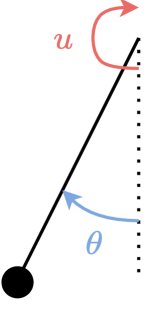
Figure 8: Fixed pendulum.

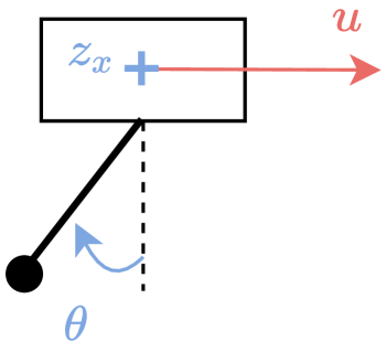
Figure 9: Pendulum on a cart.

10.2.2 Pendulum on a Cart

We consider here controlling a pendulum on a cart as illustrated in Fig. 9. This system is described by the angle $\theta$ of the pendulum with the vertical and the position $z_{x}$ of the cart on the horizontal axis. Contrary to the previous example, here we do not control directly the angle of the pendulum we only control the system with a force $u$ that drives the acceleration of the cart. The dynamics of the system satisfy (see Magdy et al., (2019) for detailed derivations)

$$(M+m)\ddot{z}_{x}+ml\cos\theta\ddot{\theta} =-b\dot{z}_{x}+ml\dot{\theta}^{2}\sin\theta+u$$

$$ml\cos\theta\ddot{z}_{x}+(I+ml^{2})\ddot{\theta} =-mgl\sin\theta,$$ (51)

where $M$ is the mass of the cart, $m$ is the mass of the pendulum rod, $I$ is the pendulum rod moment of inertia, $l$ is the length of the rod, and $b$ is the viscous friction coefficient of the cart. The system of equations can be written in matrix form and solved to express the angle and position accelerations as

$$\left(\begin{matrix}\ddot{z}_{x}\\ \ddot{\theta}\end{matrix}\right) =\left(\begin{matrix}M+m&ml\cos\theta\\ ml\cos\theta&I+ml^{2}\end{matrix}\right)^{-1}\left(\begin{matrix}-b\dot{z}_{x}+ml\dot{\theta}^{2}\sin\theta+u\\ -mgl\sin\theta\end{matrix}\right)$$

$$=\frac{1}{I(M+m)+ml^{2}M+m^{2}l^{2}\sin^{2}\theta}\left(\begin{matrix}I+ml^{2}&-ml\cos\theta\\ -ml\cos\theta&M+m\end{matrix}\right)\left(\begin{matrix}-b\dot{z}_{x}+ml\dot{\theta}^{2}\sin\theta+u\\ -mgl\sin\theta\end{matrix}\right).$$

The discrete dynamical system follows using an Euler discretization scheme or a Runge Kutta method. We consider the task of swinging up the pendulum and keeping it vertical for a few time steps while constraining the movement of the cart on the horizontal line. Formally, we consider the following cost, defined for $x_{t}=(z_{x},\theta,\zeta_{x},\omega)$, where $\zeta_{x},\omega$ represent the discretizations of $\dot{z}_{x}$ and $\dot{\theta}$ respectively,

$$h(x_{t},u_{t}) =\begin{cases}\rho_{2}(\max(z_{x}-\bar{z}_{x}^{+},0)+\max(z_{x}+\bar{z}_{x}^{-},0))+\lambda u_{t}^{2}+(\theta+\pi)^{2}+\rho_{1}\omega^{2}&\mbox{if}\ t\geq\bar{t}\\ \rho_{2}(\max(z_{x}-\bar{z}_{x}^{+},0)+\max(z_{x}+\bar{z}_{x}^{-},0))+\lambda u_{t}^{2}&\mbox{if}\ t<\bar{t},\end{cases}$$

where $\rho_{1},\rho_{2},\lambda$ are some non-negative parameters, $\bar{t}$ is a time step after which the pendulum needs to stay vertically inverted and $\bar{z}_{x}^{+},\bar{z}_{x}^{-}$ are bounds that restrain the movement of the cart along the whole horizontal line.

10.3 Autonomous Car Racing

We consider the control of a car on a track through two different dynamical models: a simple one where the orientation of the car is directly controlled by the steering angle, and a more realistic one that takes into account the tire forces to control the orientation of the car. In the following, we present the dynamics, a simple tracking cost, and a contouring cost enforcing the car to race the track at a reference speed or as fast as possible.

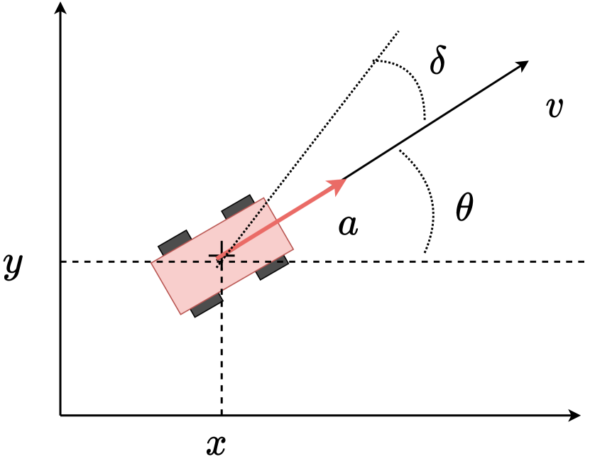
Figure 10: Simple model of a car.

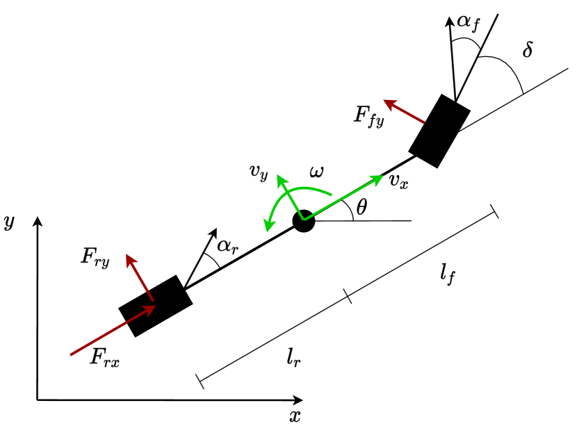
Figure 11: Bicycle model of a car.

10.3.1 Dynamics

Simple model

A simple model of the car is described in Fig. 11. The state of the car is decomposed as $z(t)=(x(t),y(t),\theta(t),v(t))$, where (dropping the dependency w.r.t. time for simplicity)

1. $x,y$ denote the position of the car on the plane,

2. $\theta$ denotes the angle between the orientation of the car and the horizontal axis, a.k.a. the yaw,

3. $v$ denotes the longitudinal speed.

The car is controlled through $u(t)=(a(t),\delta(t))$, where

1. $a$ is the longitudinal acceleration of the car,

2. $\delta$ is the steering angle.

For a car of length $L$, the continuous time dynamics are then

$$\dot{x}=v\cos\theta\qquad\dot{y}=v\sin\theta\qquad\dot{\theta}=v\tan(\delta)/L\qquad\dot{v}=a.$$ (52)

Bicycle model

We consider the model presented by Liniger et al., (2015) recalled below and illustrated in Fig. 11. In this model, the state of the car at time $t$ is decomposed as $z(t)=(x(t),y(t),\theta(t),v_{x}(t),v_{y}(t),\omega(t))$ where

1. $x,y$ denote the position of the car on the plane,

2. $\theta$ denotes the angle between the orientation of the car and the horizontal axis, a.k.a. the yaw,

3. $v_{x}$ denotes the longitudinal speed,

4. $v_{y}$ denotes the lateral speed,

5. $\omega$ denotes the derivative of the orientation of the car, a.k.a. the yaw rate.

The control variables are analogous to the simple model, i.e., $u(t)=(a(t),\delta(t))$, where

1. $a$ is the PWM duty cycle of the car, this duty cycle can be negative to take into account braking,

2. $\delta$ is the steering angle.

These controls act on the state through the following forces.

1. A longitudinal force on the rear wheels, denoted $F_{r,x}$ modeled using a motor model for the DC electric motor as well as a friction model for the rolling resistance and the drag

   $$F_{r,x}=(C_{m1}-C_{m2}v_{x})a-C_{r0}-C_{rd}v_{x}^{2}$$

   where $C_{m1},C_{m2},C_{r0},C_{rd}$ are constants estimated from experiments, see Appendix A.

2. Lateral forces on the front and rear wheels, denoted $F_{f,y},F_{y,r}$ respectively, modeled using a simplified Pacejka tire model

   $$F_{f,y} =D_{f}\sin(C_{f}\arctan(B_{f}\alpha_{f}))\quad\textrm{where}\ \alpha_{f}=\delta-\operatorname{arctan2}\left(\frac{\omega l_{f}+v_{y}}{v_{x}}\right)$$

   $$F_{r,y} =D_{r}\sin(C_{r}\arctan(B_{r}\alpha_{r}))\quad\textrm{where}\ \alpha_{r}=\operatorname{arctan2}\left(\frac{\omega l_{r}-v_{y}}{v_{x}}\right)$$

   where $\alpha_{f}$, $\alpha_{r}$ are the slip angles on the front and rear wheels respectively, $l_{f},l_{r}$ are the distance from the center of gravity to the front and the rear wheel respectively and the constants $B_{r},C_{r},D_{r},B_{f},C_{f},D_{f}$ define the exact shape of the semi-empirical curve, presented in Fig. 12.

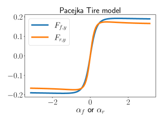
Figure 12: Pacejka model of the friction on the tires as a function of the slip angles

The continuous time dynamics are then

$$\dot{x} =v_{x}\cos\theta-v_{y}\sin\theta \dot{v}_{x} =\frac{1}{m}(F_{r,x}-F_{f,y}\sin\delta)+v_{y}\omega$$ (53)

$$\dot{y} =v_{x}\sin\theta+v_{y}\cos\theta \dot{v}_{y} =\frac{1}{m}(F_{r,y}+F_{f,y}\cos\delta)-v_{x}\omega$$

$$\dot{\theta} =\omega \dot{\omega} =\frac{1}{I_{z}}(F_{f,y}l_{f}\cos\delta-F_{r,y}l_{r}),$$

where $m$ is the mass of the car and $I_{z}$ is the inertia.

10.3.2 Costs

Tracks

We consider tracks that are given as a continuous curve, namely a cubic spline approximating a set of points. As a result, for any time $t$, we have access to the corresponding point $\hat{x}(t),\hat{y}(t)$ on the curve. The track we consider is a simple track illustrated in Fig. 13.

Tracking cost

A simple cost on the states is

$$c_{t}(z_{t})=\|x_{t}-\hat{x}(\Delta v^{\textrm{ref}}t)\|_{2}^{2}+\|y_{t}-\hat{y}(\Delta v^{\textrm{ref}}t)\|_{2}^{2}\quad\mbox{for}\ t=1,\ldots,\tau,$$ (54)

for $z_{t}=(x_{t},y_{t})$, where $\Delta$ is some discretization step and $v^{\textrm{ref}}$ is some reference speed. The cost above is the one we choose for the simple model of a car. The disadvantage of such a cost is that it enforces the car to follow the track at a constant speed which may not be physically possible. We consider in the following a contouring cost as done by Liniger et al., (2015).

Ideal cost

Given a track parameterized in continuous time, an ideal cost is to enforce the car to be as close as possible to the track, while moving along the track as fast as possible. Formally, define the distance from the car at position $(x,y)$ to the track defined by the curve $\hat{x}(t),\hat{y}(t)$ as

$$d(x,y)=\min_{t\in{\mathbb{R}}}\quad\sqrt{((x-\hat{x}(t))^{2}+(y-\hat{y}(t))^{2}}.$$

Denoting $t^{*}=t(x,y)=\operatorname*{arg\,min}_{t\in{\mathbb{R}}}\quad(x-\hat{x}(t))^{2}+(y-\hat{y}(t))^{2},$ the reference time on the track for a car at position $(x,y)$, the distance $d(x,y)$ can be expressed as

$$d(x,y)=\sin(\theta(t^{*}))\left(x-\hat{x}(t^{*})\right)-\cos(\theta(t^{*}))\left(y-\hat{y}(t^{*})\right),$$

where $\theta(t)=\frac{\partial\hat{y}(t)}{\partial\hat{x}(t)}$ is the angle of the track with the x-axis. The distance $d(x,y)$ is illustrated in Fig. 16. An ideal cost for the problem is then defined as $h(z)=h(x,y)=d(x,y)^{2}-t(x,y),$ which enforces the car to be close to the track by minimizing $d(x,y)^{2}$, and also encourages the car to go as far as possible by adding the term $-t(x,y)$.

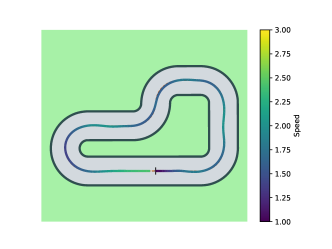
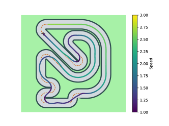
Figure 13: Simple and complex tracks used with a trajectory computed on the bicycle model (53).

Contouring and lagging costs

The computation of $t^{*}$ involves solving an optimization problem and is not practical. As Liniger et al., (2015), we rather augment the states with a flexible reference time. Namely, we augment the state of the car by adding a variable $s$ whose objective is to approximate the reference time $t^{*}$. The cost is then decomposed into the contouring cost and the lagging cost illustrated in Fig. 16 and defined as

$$e_{c}(x,y,s) =\sin(\theta(s))\left(x-\hat{x}(s)\right)-\cos(\theta(s))\left(y-\hat{y}(s)\right)$$

$$e_{l}(x,y,s) =-\cos(\theta(s))\left(x-\hat{x}(s)\right)-\sin(\theta(s))\left(y-\hat{y}(s)\right).$$

Rather than encouraging the car to make the most progress on the track, we enforce them to keep a reference speed. Namely we consider an additional penalty of the form $\|\dot{s}-v^{\textrm{ref}}\|_{2}^{2}$ where $v^{\textrm{ref}}$ is a parameter chosen in advance. For the reference time $s$ not to go backward in time, we add a log-barrier term $-\varepsilon\log(\dot{s})$ for $\varepsilon=10^{-6}$.

Finally, we let the system control the reference time through its second order derivative $\ddot{s}$. Overall this means that we augment the state variable by adding the variables $s$ and $\nu:=v_{s}$ and that we augment the control variable by adding the variable $\alpha:=a_{s}$ such that the discretized problem is written for, e.g., the bicycle model, as

$$\min_{\begin{subarray}{c}(a_{0},\delta_{0},\alpha_{0}),\ldots,(a_{\tau-1},\delta_{\tau-1},\alpha_{\tau-1}\end{subarray})}\quad \sum_{t=0}^{\tau-1}\rho_{c}e_{c}(x_{t},y_{t},s_{t})^{2}+\rho_{l}e_{l}(x_{t},y_{t},s_{t})^{2}+\rho_{v}\|v_{s,t}-v^{\textrm{ref}}\|_{2}^{2}-\varepsilon\log\nu_{t}$$

s.t. $$x_{t+1},y_{t+1},\theta_{t+1},v_{x,t+1},v_{y,t+1},\omega_{t+1}=f(x_{t},y_{t},\theta_{,}v_{x,t},v_{y,t},\omega_{t},\delta_{t},a_{t})$$

$$s_{t+1}=s_{t}+\Delta\nu_{t},\quad\nu_{t+1}=\nu_{t}+\Delta\alpha_{t}$$

$$z_{0}=\hat{z}_{0}\quad s_{0}=0\quad\nu_{0}=v^{\textrm{ref}},$$

where $f$ is a discretization of the continuous time dynamics, $\Delta$ is a discretization step and $\hat{z}_{0}$ is a given initial state where $z_{0}$ regroups all state variables at time 0 (i.e. all variables except $a_{0},\delta_{0}$).

This cost is defined by the parameters $\rho_{c},\rho_{l},\rho_{v},v^{\textrm{ref}}$ which are fixed in advance. The larger the parameter $\rho_{c}$, the closer the car to the track. The larger the parameter $\rho_{l}$, the closer the car to its reference time $s$. In practice, we want the reference time to be a good approximation of the ideal projection of the car on the track so $\rho_{l}$ should be chosen large enough. On the other hand, varying $\rho_{c}$ allows having a car that is either conservative and potentially slow or a car that is fast but inaccurate, i.e., far from the track. The most important aspect of the trajectory is to ensure that the car remains inside the borders of the track defined in advance.

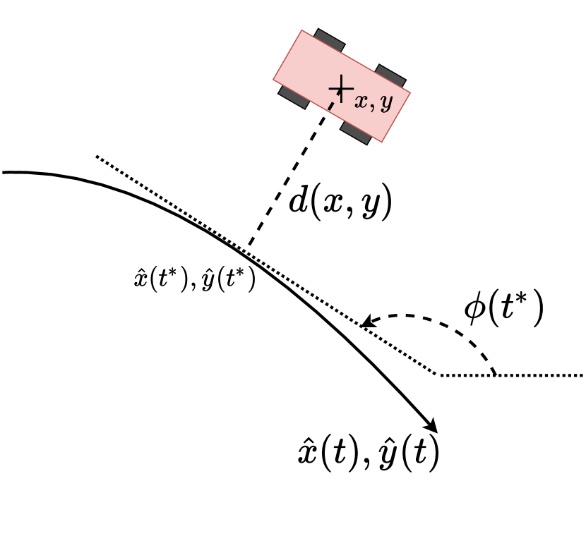
Figure 14: Distance to the track.

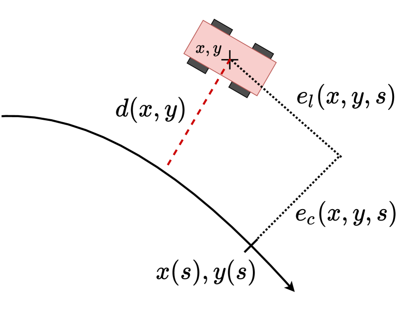
Figure 15: Approx. by contouring and lagging costs.

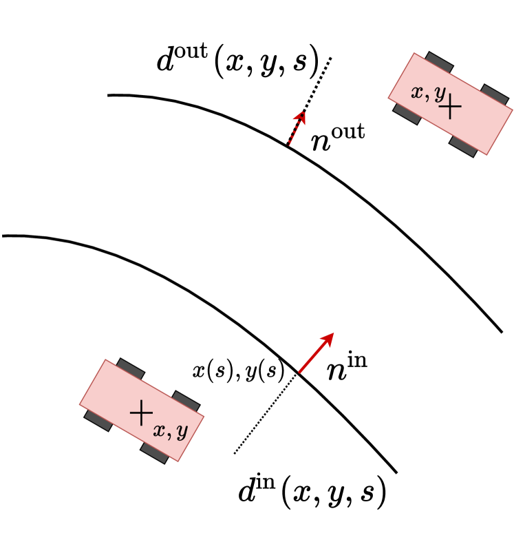
Figure 16: Border costs.

Border costs

To enforce the car to remain inside the track defined by some borders, we penalize the approximated distance of the car to the border when it goes outside the border as $e_{b}(x,y,s)=e_{b}^{\textrm{in}}(x,y,s)+e_{b}^{\textrm{out}}(x,y,s)$ with

$$e_{b}^{\textrm{in}}(x,y,s) =\max((w+d^{\textrm{in}}(x,y,s))^{2},0) d^{\textrm{in}}(x,y,s) =-(z-z^{\textrm{in}}(s))^{\top}n^{\textrm{in}}(s)$$ (55)

$$e_{b}^{\textrm{out}}(x,y,s) =\max((w+d^{\textrm{out}}(x,y,s))^{2},0) d^{\textrm{out}}(x,y,s) =(z-z^{\textrm{out}}(s))^{\top}n^{\textrm{out}}(s)$$

for $z=(x,y)$, where $n^{\textrm{in}}(s)$ and $n^{\textrm{out}}(s)$ denote the normal at the borders at time $s$ and $w$ is the width of the car. In practice, we use a smooth approximation of the max function in Eq. (55). The normals $n^{\textrm{in}}(s)$ and $n^{\textrm{out}}(s)$ can easily be computed by derivating the curves defining the inner and outer borders. These costs are illustrated in Fig. 16.

Constrained controls

We constrain the steering angle to be between $[-\pi/3,\pi/3]$ by parameterizing the steering angle as

$$\delta(\tilde{\delta})=\frac{2}{3}\arctan(\tilde{\delta})\quad\mbox{for}\ \tilde{\delta}\in{\mathbb{R}}.$$

Similarly, we constrain the acceleration $a$ to be between $[c,d]$ (with $c=-0.1,d=1.$), by parameterizing it as

$$a(\tilde{a})=(d-c)\operatorname{sig}(4\tilde{a}/(d-c))+c$$

with $\operatorname{sig}:x\rightarrow 1/(1+e^{-x})$ the sigmoid function. The final set of control variables is then $\tilde{a},\tilde{\delta},\alpha$.

Control costs

For both trajectory costs, we add a square regularization on the control variables of the system, i.e., the cost on the control variables is $\lambda\|u_{t}\|_{2}^{2}$ for some $\lambda\geq 0$ where $u_{t}$ are the control variables at time $t$.

Overall contouring cost

The whole problem with contouring cost is then

$$\min_{\begin{subarray}{c}(\tilde{a}_{0},\tilde{\delta}_{0},\alpha_{0}),\ldots,(\tilde{a}_{\tau-1},\tilde{\delta}_{\tau-1},\tilde{\alpha}_{\tau-1}\end{subarray})}\quad \sum_{t=0}^{\tau-1}\Big{[}\rho_{c}e_{c}(x_{t},y_{t},s_{t})^{2}+\rho_{l}e_{l}(x_{t},y_{t},s_{t})^{2}+\rho_{v}\|v_{s,t}-v^{\textrm{ref}}\|_{2}^{2}-\varepsilon\log(\nu_{t})$$

$$\qquad+\rho_{b}e_{b}(x_{t},y_{t},s_{t})^{2}+\lambda(\tilde{a}_{t}^{2}+\tilde{\delta}_{t}^{2}+\alpha_{t}^{2})\Big{]}$$ (56)

s.t. $$x_{t+1},y_{t+1},\theta_{t+1},v_{x,t+1},v_{y,t+1},\omega_{t+1}=f(x_{t},y_{t},\theta_{t},v_{x,t},v_{y,t},\omega_{t},\delta_{t}(\tilde{\delta}_{t}),a_{t}(\tilde{a}_{t}))$$

$$s_{t+1}=s_{t}+\Delta\nu_{t},\quad\nu_{t+1}=\nu_{t}+\Delta\alpha_{t}$$

$$z_{0}=\hat{z}_{0}\quad s_{0}=0\quad\nu_{0}=v^{\textrm{ref}},$$

with parameters $\rho_{c},\rho_{l},\rho_{v},v^{\textrm{ref}},\rho_{b},\lambda$ and $f$ given in Eq. (53).

10.4 Results

All the following plots are in log-scale where on the vertical axis we plot $\log\left((\mathcal{J}({{\bm{u}}^{(k)}})-\mathcal{J}^{*})/(\mathcal{J}({\bm{u}}^{(0)})-\mathcal{J}^{*})\right)$ with $\mathcal{J}$ the objective, ${{\bm{u}}^{(k)}}$ the set of controls at iteration $k$, and $\mathcal{J}^{*}=\min_{{\bm{u}}\in{\mathbb{R}}^{\tau{n_{u}}}}\mathcal{J}({\bm{u}})$ estimated from running the algorithms for more iterations than presented. The acronyms (GD, GN, NE, DDP-LQ, DDP-Q) correspond to the taxonomy of algorithms presented in Fig. 2. For the bicycle model of a car, gradient oracles appeared numerically unstable for moderate horizons, probably due to the highly nonlinear modeling of the tire forces, hence we do not plot GD for that example. Finally the algorithms are stopped if the stepsizes found by line-search are smaller than $10^{-20}$ or if the relative difference in terms of costs is smaller than $10^{-12}$. The algorithms are run with double precision.

10.4.1 Linear Quadratic Approximations

In Fig. 17, we compare a gradient descent and nonlinear control algorithms with linear quadratic approximations, i.e., GN or DDP-LQ with directional or regularized steps.

1. We observe that GN and DDP-LQ always outperform GD.

2. Similarly, we observe that DDP generally outperforms GN, for the same steps (directional or regularized), except for the simple model of a car where a GN method with directional steps appears better than its DDP counterpart.

3. For GN, taking a directional step can be better than taking regularized steps for easy problems such as the fixed pendulum or the simple model of a car. The regularized steps can be advantageous for harder problems as illustrated in the control of a bicycle model of a car or the pendulum on a cart.

4. For DDP, regularized steps generally outperform directional steps and all other algorithms. An exception is the control of a pendulum on a cart where DDP with directional steps may suddenly obtain a good solution, once close enough to the minimum, while DDP with regularized steps may stay stuck.

In Fig. 18, we plot the same algorithms but with respect to time.

1. We observe that in terms of time, the regularized steps may require fewer evaluations during the line-search as they incorporate previous stepsizes and may provide faster convergence in time.

2. On the other hand, as previously mentioned, by initializing the line-search of the directional steps at $1$, we may observe sudden convergence as illustrated in the control of a pendulum on a cart.

Finally, in Fig. 19, we plot the stepsizes taken by the algorithms for the pendulum and the simple model of a car.

1. On the pendulum example, the stepsizes used by directional steps quickly tend to $1$ which means that the algorithms (GN or DDP-LQ) are then taking the largest possible stepsize for this strategy and may exhibit quadratic convergence.

2. On the other hand, for the regularized steps, on the pendulum example, the regularization (i.e. the inverse of the stepsizes) quickly converges to $0$, which means that, as the number of iterations increases, the regularized and directional steps coincide.

3. For the car example, the step sizes for the directional steps never converge exactly to one, which may explain the slower convergence. For the regularized steps, on the horizons $\tau=25$ or $50$ we observe again that DDP uses increasingly larger stepsizes which corroborate its performance on this problem.

10.4.2 Quadratic Approximations

In Fig. 17, we compare nonlinear control algorithms with quadratic approximations, i.e., NE or DDP-Q with different steps.

1. Here the regularized version of the classical oracle, i.e., Newton, rarely outperforms its counterpart with descent direction.

2. Overall, DDP methods always outperform their NE counterparts.

3. As with the linear quadratic approximations, the DDP approach with directional steps outperforms the regularized step version for the pendulum on a cart. On the other hand, DDP with regularized steps is better for the bicycle model of a car and a short horizon of the simple model of a car.

In Fig 21, we plot the same algorithms but in time.

1. Here we observe no particular difference with the plots in iteration, i.e., the search with regularized steps does not lead to much more favorable line-search time.

2. We observe that DDP-Q is comparable in computational time to DDP-LQ for the fixed pendulum and the simple model of a car. On the other hand, for the bicycle model of a car, DDP-Q may be much slower.

3. Generally NE does not compare favorably to its linear-quadratic counterpart.

In Fig. 22, we compare the stepsizes taken by the methods.

1. In terms of directional steps, DDP-Q appears to take relatively large steps while its NE counterpart may have more variations.

2. We observe clearly in these plots that the regularized version of NE is not able to take small regularization constants, which explains its poor performance. On the other hand, DDP-Q with regularized steps tends to quickly take small regularizations (large stepsizes).

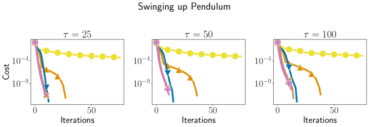
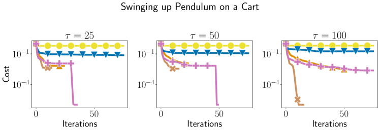
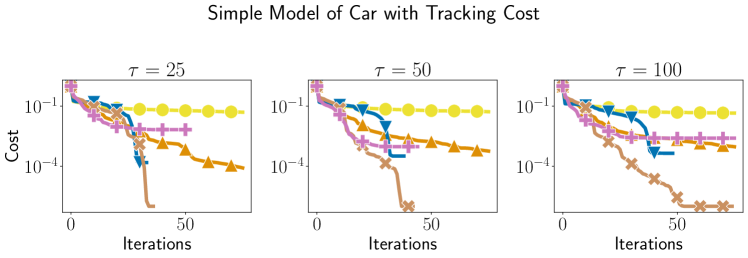
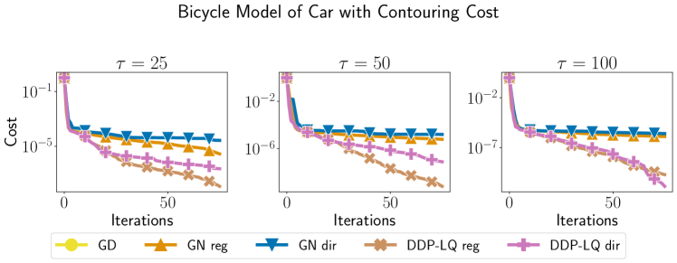
Figure 17: Convergence of algorithms with linear quadratic approximations in iterations.

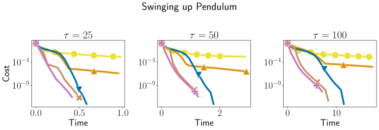
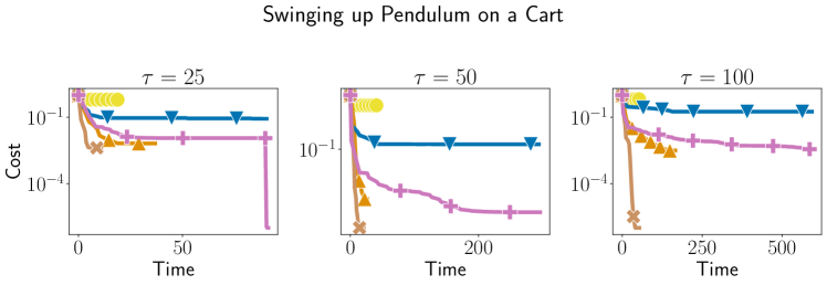
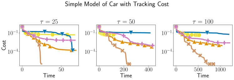
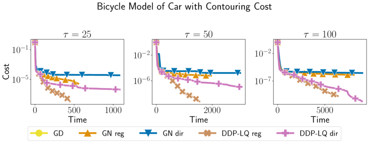
Figure 18: Convergence of algorithms with linear quadratic approximations in time.

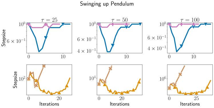
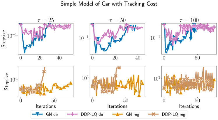
Figure 19: Stepsizes taken along the iterations for linear quadratic approximations.

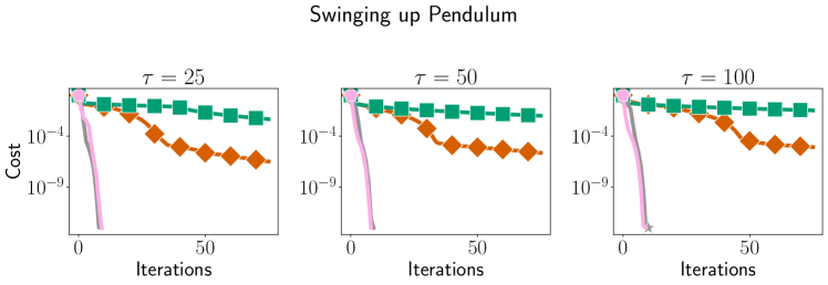
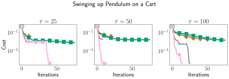
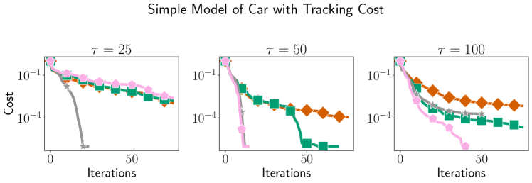
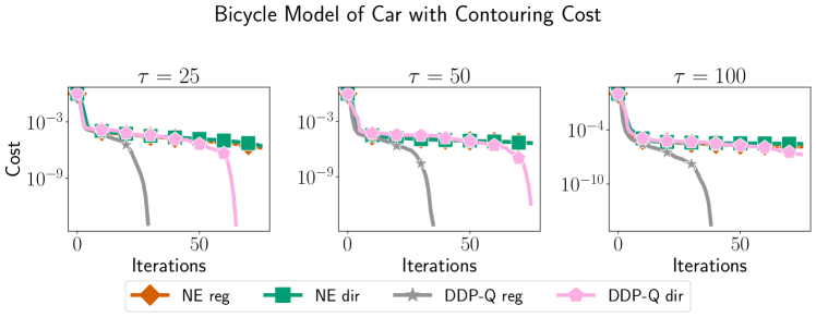
Figure 20: Convergence of algorithms with quadratic approximations in iterations.

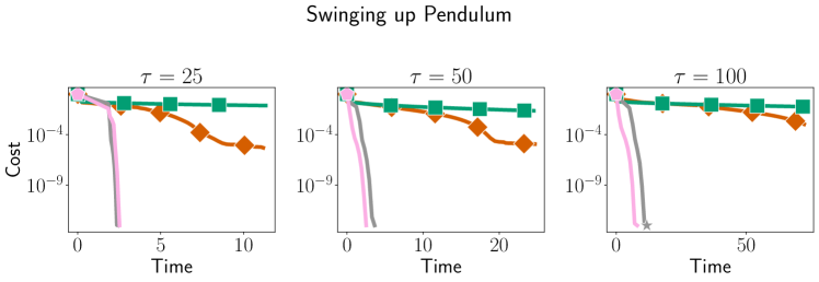
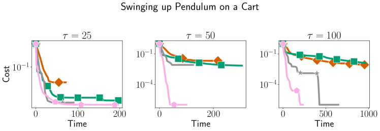
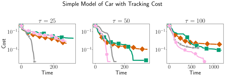
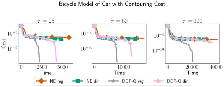
Figure 21: Convergence of algorithms with quadratic approximations in time.

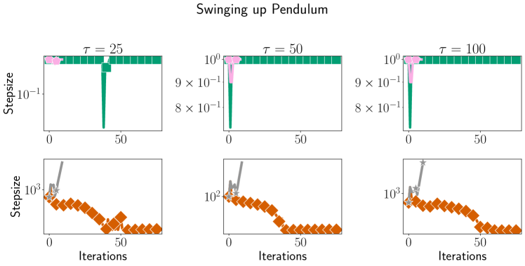
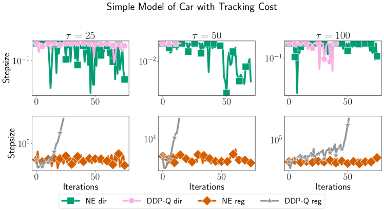
Figure 22: Stepsizes taken along the iterations for quadratic approximations.

Acknowledgments

This work was supported by NSF DMS-1839371, DMS-2134012, CCF-2019844, CIFAR-LMB, NSF TRIPODS II DMS-2023166 and faculty research awards. The authors deeply thank Alexander Liniger for his help on implementing the bicycle model of a car. The authors also thank Dmitriy Drusvyatskiy, Krishna Pillutla and John Thickstun for fruitful discussions on the paper and the code.

Appendix A Experimental Details

The code is available at https://github.com/vroulet/ilqc. We add for ease of reference, the hyper-parameters used for each setting.

Pendulum

1. mass $m=1$,

2. gravitational constant $g=10$,

3. length of the blob $l=1$,

4. friction coefficient $\mu=0.01$,

5. speed regularization $\lambda=0.1$,

6. control regularization $\rho=10^{-6}$,

7. total time of the movement $T=2$, discretization step $\Delta=T/\tau$ for varying $\tau$

8. Euler discretization scheme.

Pendulum on a cart

1. mass of the rod $m=0.2$,

2. mass of the cart $M=0.5$,

3. viscous coefficient $b=0.1$,

4. moment of inertia $I=0.006$,

5. length of the rod $0.3$,

6. speed regularization $\lambda_{1}=0.1$,

7. barrier parameter $\rho_{2}=1.$,

8. control regularization $\rho=10^{-6}$,

9. total time of the movement $T=2.5$, discretization step $\Delta=T/\tau$ for varying $\tau$,

10. stay put time $\bar{t}=\tau-\lfloor 0.6/\Delta\rfloor$,

11. barriers $\bar{z}^{+}=2$, $\bar{z}^{-}=-2$,

12. Euler discretization scheme.

Simple car with tracking cost

1. length of the car $L=1$,

2. reference speed $v^{ref}=3$,

3. initial speed $v^{init}=1$,

4. control regularization $\lambda=10^{-6}$,

5. total time of the movement $T=2$,

6. simple track,

7. Euler discretization scheme.

Bicycle model of a car with a contouring objective

1. $C_{m1}=0.287$, $C_{m2}=0.0545$,

2. $C_{r0}=0.0518$, $C_{rd}=0.00035$,

3. $B_{r}=3.3852$, $C_{r}=1.2691$, $D_{r}=0.1737$, $l_{r}=0.033$

4. $B_{f}=2.579$, $C_{f}=1.2$, $D_{f}=0.192$, $l_{f}=0.029$

5. $m=0.041$, $I_{z}=27.8\cdot 10^{-6}$

6. contouring error penalty $\rho_{c}=0.1$,

7. lagging error penalty $\rho_{l}=10$,

8. reference speed penalty $\rho_{v}=0.1$,

9. barrier error penalty $\rho_{b}=100$,

10. reference speed $v^{\textrm{ref}}=3$,

11. initial speed $v^{init}=1$,

12. control regularization $\lambda=10^{-6}$,

13. total time of the movement $T=1$,

14. simple track,

15. Runge-Kutta discretization scheme.

References

- Arrow, (1968) Arrow, K. (1968). Applications of control theory to economic growth. In Lectures on Applied Mathematics, volume 12 (Mathematic of the Decision Science, Part 2).
- Arutyunov and Vinter, (2004) Arutyunov, A. V. and Vinter, R. B. (2004). A simple ‘finite approximations’ proof of the Pontryagin maximum principle under reduced differentiability hypotheses. Set-valued analysis, 12(1):5–24.
- Bellman, (1971) Bellman, R. (1971). Introduction to the mathematical theory of control processes, volume 2. Academic press.
- Bertsekas, (1976) Bertsekas, D. (1976). Dynamic Programming and Stochastic Control. Academic Press.
- Bertsekas, (2016) Bertsekas, D. (2016). Nonlinear Programming, volume 4. Athena Scientific.
- Betts, (2010) Betts, J. (2010). Practical methods for optimal control and estimation using nonlinear programming. SIAM.
- Boyd and Vandenberghe, (1997) Boyd, S. and Vandenberghe, L. (1997). Semidefinite programming relaxations of non-convex problems in control and combinatorial optimization. In Communications, Computation, Control, and Signal Processing, pages 279–287. Springer.
- Clarke, (1979) Clarke, F. (1979). Optimal control and the true Hamiltonian. SIAM Review, 21(2):157–166.
- Dunn and Bertsekas, (1989) Dunn, J. and Bertsekas, D. (1989). Efficient dynamic programming implementations of Newton’s method for unconstrained optimal control problems. Journal of Optimization Theory and Applications, 63(1):23–38.
- Griewank and Walther, (2008) Griewank, A. and Walther, A. (2008). Evaluating derivatives: principles and techniques of algorithmic differentiation. SIAM.
- Jacobson and Mayne, (1970) Jacobson, D. and Mayne, D. (1970). Differential Dynamic Programming. Elsevier.
- Kamien and Schwartz, (1971) Kamien, M. and Schwartz, N. (1971). Sufficient conditions in optimal control theory. Journal of Economic Theory, 3(2):207–214.
- Lewis, (2006) Lewis, A. D. (2006). The maximum principle of Pontryagin in control and in optimal control. Handouts for the course taught at the Universitat Politecnica de Catalunya.
- Li and Todorov, (2007) Li, W. and Todorov, E. (2007). Iterative linearization methods for approximately optimal control and estimation of non-linear stochastic system. International Journal of Control, 80(9):1439–1453.
- Liao and Shoemaker, (1991) Liao, L.-Z. and Shoemaker, C. (1991). Convergence in unconstrained discrete-time differential dynamic programming. IEEE Transactions on Automatic Control, 36(6):692–706.
- Liao and Shoemaker, (1992) Liao, L.-Z. and Shoemaker, C. A. (1992). Advantages of differential dynamic programming over Newton’s method for discrete-time optimal control problems. Technical report, Cornell University.
- Liniger et al., (2015) Liniger, A., Domahidi, A., and Morari, M. (2015). Optimization-based autonomous racing of 1: 43 scale RC cars. Optimal Control Applications and Methods, 36(5):628–647.
- Magdy et al., (2019) Magdy, M., El Marhomy, A., and Attia, M. A. (2019). Modeling of inverted pendulum system with gravitational search algorithm optimized controller. Ain Shams Engineering Journal, 10(1):129–149.
- Mangasarian, (1966) Mangasarian, O. (1966). Sufficient conditions for the optimal control of nonlinear systems. SIAM Journal on Control, 4(1):139–152.
- Mayne and Polak, (1975) Mayne, D. and Polak, E. (1975). First-order strong variation algorithms for optimal control. Journal of Optimization Theory and Applications, 16(3):277–301.
- Murray and Yakowitz, (1984) Murray, D. and Yakowitz, S. (1984). Differential dynamic programming and Newton’s method for discrete optimal control problems. Journal of Optimization Theory and Applications, 43(3):395–414.
- Nganga and Wensing, (2021) Nganga, J. and Wensing, P. (2021). Accelerating second-order differential dynamic programming for rigid-body systems. IEEE Robotics and Automation Letters, 6(4):7659–7666.
- Nocedal and Wright, (2006) Nocedal, J. and Wright, S. (2006). Numerical optimization. Springer Science & Business Media.
- Pantoja, (1988) Pantoja, J. (1988). Differential dynamic programming and Newton’s method. International Journal of Control, 47(5):1539–1553.
- Pontryagin et al., (1963) Pontryagin, L., Boltyansky, V., Gamkrelidze, R., and Mischenko, E. (1963). The mathematical theory of optimal processes. Wiley-Interscience.
- Rao et al., (1998) Rao, C., Wright, S., and Rawlings, J. (1998). Application of interior-point methods to model predictive control. Journal of optimization theory and applications, 99(3):723–757.
- Roulet et al., (2019) Roulet, V., Srinivasa, S., Drusvyatskiy, D., and Harchaoui, Z. (2019). Iterative linearized control: stable algorithms and complexity guarantees. In Proceedings of the 36th International Conference on Machine Learning, pages 5518–5527.
- Roulet et al., (2022) Roulet, V., Srinivasa, S., Fazel, M., and Harchaoui, Z. (2022). Complexity bounds of iterative linear quadratic optimization algorithms for discrete time nonlinear control. arXiv preprint arXiv:2204.02322.
- Sideris and Bobrow, (2005) Sideris, A. and Bobrow, J. (2005). An efficient sequential linear quadratic algorithm for solving nonlinear optimal control problems. In Proceedings of the 2005 American Control Conference, pages 2275–2280.
- Tassa et al., (2012) Tassa, Y., Erez, T., and Todorov, E. (2012). Synthesis and stabilization of complex behaviors through online trajectory optimization. In 2012 IEEE/RSJ International Conference on Intelligent Robots and Systems, pages 4906–4913.
- Tassa et al., (2014) Tassa, Y., Mansard, N., and Todorov, E. (2014). Control-limited differential dynamic programming. In 2014 IEEE International Conference on Robotics and Automation (ICRA), pages 1168–1175.
- Todorov et al., (2012) Todorov, E., Erez, T., and Tassa, Y. (2012). Mujoco: A physics engine for model-based control. In International Conference on Intelligent Robots and Systems (IROS), pages 5026–5033. IEEE.
- Wright, (1990) Wright, S. (1990). Solution of discrete-time optimal control problems on parallel computers. Parallel Computing, 16(2-3):221–237.
- (34) Wright, S. (1991a). Partitioned dynamic programming for optimal control. SIAM Journal on optimization, 1(4):620–642.
- (35) Wright, S. (1991b). Structured interior point methods for optimal control. In Proceedings of the 30th IEEE Conference on Decision and Control, pages 1711–1716.