Two-dimensional delta-Bose gas: skew-product relative motion and exact non-Gaussianity for the stochastic heat equation

Abstract

For the two-dimensional delta-Bose gas, we prove the first Feynman–Kac type diffusion representation of the Schrödinger semigroup generated by the relative motion of two particles. The representation builds on a unique skew-product diffusion, in the sense of Erickson [22], such that the Markov process ${\rm BES}(0,\beta{\downarrow})$ from Donati-Martin and Yor [20] defines the radial part. Moreover, the law of this skew-product diffusion is singular to the law of planar Brownian motion. As an application, we determine some exact forms of non-Gaussianity for the stochastic heat equation. We give two different proofs of the representation: one applies the original characterization of ${\rm BES}(0,\beta{\downarrow})$ by excursion theory, and the other extends [20] by approximations of SDEs and resolvents. In the latter, we establish a new characterization of ${\rm BES}(0,\beta{\downarrow})$ as a strongly well-posed SDE. The approximations of resolvents construct the two-dimensional delta potentials from local times of lower-dimensional Bessel processes, which may be of independent interest for being an alternative to the long-standing approach of using mollifiers.

Keywords: Delta-Bose gas; Schrödinger operators; Bessel processes; gamma subordinator; Krein’s string; self-adjoint extensions; stochastic heat equation; random polymers.

Mathematics Subject Classification (2000): 60J55, 60J65, 60H30.

1 Introduction

The main objective of this paper is to establish and describe a diffusion representation of the following Hamiltonian for a one-body quantum mechanical model:

$$\mathscr{L}\,{\stackrel{{\scriptstyle\rm def}}{{=}}}-\Delta_{z}-\Lambda\delta(z),\quad z\in\mathbb{C}.$$ (1.1)

Here, $\Delta_{z}$ denotes the Laplacian with respect to $z$, and the coupling constant $\Lambda$ and the delta function $\delta(\cdot)$ altogether symbolically describe two particles coupled by a delta-like interaction. One of our main motivations for investigating the above Hamiltonian is that it defines the “contact interaction” of any two particles in the broader context of the so-called two-dimensional delta-Bose gas. The latter has Hamiltonian given by:

$$\mathscr{H}\,{\stackrel{{\scriptstyle\rm def}}{{=}}}-\frac{1}{2}\sum_{j=1}^{N}\Delta_{z_{j}}-\Lambda\sum_{j<k}\delta(z_{k}-z_{j}),$$ (1.2)

where $z_{j}\in\mathbb{C}$ stands for the position of the $j$-th particle. The simplest relation between (1.1) and (1.2) occurs when there are only two particles in the delta-Bose gas. In this case, a straightforward change of variables shows that $\mathscr{L}$ describes the dynamics of the relative motion $z=z_{2}-z_{1}$, and the complementary dynamics are the Laplacian $\Delta_{z^{\prime}}/4$ satisfied by the center of mass $z^{\prime}=(z_{2}+z_{1})/2$. Specifically, as in [6], we write

$$\mathscr{H}=U^{-1}[(\Delta_{z^{\prime}}/4)\otimes\mathds{1}+\mathds{1}\otimes\mathscr{L}]U\quad\mbox{($N=2$)},$$ (1.3)

where $Uf(z_{1},z_{2})=f(z^{\prime},z)$. Henceforth, the relative motion refers to $\mathscr{L}$.

More precise relations between the relative motion and the many-body delta-Bose gas ($N\geq 3$) also exist, not just in the case of two particles. In the original quantum mechanical context, these relations have appeared in the functional analytic construction, first by Dell’Antonio, Figari and Teta [18] and then by Dimock and Rajeev [19] for an extension. The relations also emerge from a very different direction, where the delta-Bose gas determines moments of the stochastic heat equation. In this context, a certain diagrammatic representation of the Schrödinger semigroup arises [12, 24, 10] and indicates the reducibility of the semigroup to the relative motion and Gaussian transition kernels. Below we will discuss the stochastic heat equation and its relation to the delta-Bose gas in more detail. Note that the Hamiltonian $\mathscr{L}$ has other extensions to Hamiltonians with many-center delta interactions. See [2] for reviews.

The construction of the relative motion is proven by Albeverio, Gesztesy, Høegh-Krohn and Holden [1], extending in depth Berezin and Faddeev [4] for the analogous Hamiltonian in three dimensions. One of the main results in [1] obtains nontrivial realizations of $\mathscr{L}$ as a one-parameter family of self-adjoint operators $\Delta_{\beta}$ with domain $\mathscr{D}(\Delta_{\beta})\subset L^{2}(\mathbb{C})$, where $\beta$ ranges over $(0,\infty)$. The explicit characterization is via the resolvents $(\Delta_{\beta}+\lambda)^{-1}$ such that the densities of the semigroup $P^{\beta}_{t}=\exp\{t\Delta_{\beta}\}$ satisfy the following formula:

$$\begin{split}\int_{0}^{\infty}{\mathrm{e}}^{-\lambda t}P^{\beta}_{t}(z,\tilde{z}){\mathrm{d}}t&=G_{\lambda}(z-\tilde{z})+\frac{4\pi}{\log(\lambda/\beta)}G_{\lambda}(z)G_{\lambda}(\tilde{z}),\quad\forall\;\lambda\in(\beta,\infty),\end{split}$$ (1.4)

where $G_{\lambda}(z)$ denotes the integral density of $(-\Delta+\lambda)^{-1}$:

$$G_{\lambda}(z)\,{\stackrel{{\scriptstyle\rm def}}{{=}}}\int_{0}^{\infty}{\mathrm{e}}^{-\lambda t}P_{2t}(z){\mathrm{d}}t$$

[1, Theorem 2.2]. Here and in what follows, we write

$$P_{t}(z,\tilde{z})=P_{t}(z-\tilde{z})\,{\stackrel{{\scriptstyle\rm def}}{{=}}}\,\frac{1}{2\pi t}\exp\left(-\frac{\lvert z-\tilde{z}\rvert^{2}}{2t}\right)$$ (1.5)

for the two-dimensional Brownian transition density.

The discrepancy between the obvious probabilistic interpretation of the relative motion and the strong functional analytic flavor from (1.4) should raise the question of whether Feynman–Kac formulas for $\{P^{\beta}_{t}\}$ exist. In this direction, the physical interpretation of the Hamiltonian $\mathscr{L}$ is most natural to start with. This is by mollifying its delta potential, an approximation scheme for $\{P^{\beta}_{t}\}$ already in [1, Theorem 2.4 on p.95]. Specifically, this scheme in [1] considers weakly attractive Hamiltonians $-\Delta_{z}-\Lambda_{\varepsilon}\phi_{\varepsilon}$ for ${\varepsilon}\searrow 0$ such that

$$\Lambda_{\varepsilon}=\Lambda_{\varepsilon}(\lambda)\,{\stackrel{{\scriptstyle\rm def}}{{=}}}\,\frac{2\pi}{\log{\varepsilon}^{-1}}+\frac{2\pi\lambda}{(\log{\varepsilon}^{-1})^{2}},\quad\phi_{\varepsilon}(z)\,{\stackrel{{\scriptstyle\rm def}}{{=}}}\,{\varepsilon}^{-2}\phi({\varepsilon}^{-1}z),$$ (1.6)

where $\lambda\in{\mathbb{R}}$ and $\phi$ is a ${\mathscr{C}}^{\infty}$-probability density with a compact support. The relation to the parameter $\beta$ is given by

$$\frac{\log\beta}{2}=-{\int\!\!\!\int}\phi(z)\phi(\tilde{z})\log\lvert z-\tilde{z}\rvert{\mathrm{d}}z{\mathrm{d}}\tilde{z}+\log 2+\lambda-\gamma_{\sf EM},$$ (1.7)

where $\gamma_{\sf EM}=0.57721...$ denotes the Euler–Mascheroni constant. In this setting, the Feynman–Kac semigroup for $-\Delta-\Lambda_{\varepsilon}\phi_{\varepsilon}$ is classical:

$${\mathrm{e}}^{\Delta+\Lambda_{\varepsilon}\phi_{\varepsilon}}f(z_{0})={\mathbb{E}}\left[\exp\left(\Lambda_{\varepsilon}\int_{0}^{t}\phi_{\varepsilon}(B_{2}(s)-B_{1}(s)){\mathrm{d}}s\right)f(B_{2}(t)-B_{1}(t))\right]$$ (1.8)

for independent two-dimensional Brownian motions $B_{1},B_{2}$ with $B_{2}(0)-B_{1}(0)=z_{0}$.

Despite its appealing accessibility, the Brownian approximations from (1.8) are quite problematic for proving an exact Feynman–Kac formula of the semigroup $\{P^{\beta}_{t}\}$. Roughly speaking, the obstruction arises if one attempts by proving weak convergences of the exponential functionals in (1.8). This is because a nonzero distributional limit of the additive functionals $\Lambda_{\varepsilon}\int_{0}^{t}\phi_{\varepsilon}(B_{2}(s)-B_{1}(s)){\mathrm{d}}s$ occurs only when $B_{1}(0)=B_{2}(0)$. The limit is the standard exponential, say $\mathbf{e}$, according to the Kallianpur–Robbins law for scaling limits of additive functionals of two-dimensional Brownian motions [29]. But in the limit of ${\varepsilon}\searrow 0$, one gets the uninformative expectation ${\mathbb{E}}[\exp\{\mathbf{e}\}]=\infty$ from (1.8) with $f\equiv 1$. Furthermore, although some explicit description of $\Delta_{\beta}$ and its domain exists in [1], it does not seem to shed light on answering the present question for $\{P^{\beta}_{t}\}$ either. Overall speaking, this question appears to fall outside of the scope of usual Feynman–Kac formulas. Note that even for the relative motion in one dimension, the Feynman–Kac formula of the Schrödinger semigroup does exist as

$${\mathbb{E}}\Bigg{[}\exp\Bigg{\{}\Lambda\int_{0}^{t}\delta_{0}(W_{2}(s)-W_{1}(s)){\mathrm{d}}s\Bigg{\}}f(W_{2}(t)-W_{1}(t))\Bigg{]}$$ (1.9)

for any constant $\Lambda$. Here, $W_{1}$ and $W_{2}$ are independent one-dimensional Brownian motions, and $\int_{0}^{t}\delta_{0}(W_{2}(s)-W_{1}(s)){\mathrm{d}}s$ denotes the local time of $W_{2}-W_{1}$ at the point 0. See also [5] for the Feynman–Kac formula of the many-body delta-Bose gas in one dimension and their connections to the stochastic heat equation.

Representation of the relative motion by a diffusion also arises from the question of representing statistical contents of the stochastic heat equation (SHE). Here, the SHE in two (space) dimensions refers to the following formal SPDE:

$$\frac{\partial X}{\partial t}(z,t)=\frac{\Delta}{2}X(z,t)+\Lambda^{1/2}X(z,t)\xi(z,t),\quad z\in\mathbb{C},$$ (1.10)

where $\xi(z,t)$ is the centered distribution-valued white noise with correlation function

$${\mathbb{E}}[\xi(z,t)\xi(\tilde{z},\tilde{t})]=\delta(z-\tilde{z})\delta(t-\tilde{t}).$$

In the physics literature, the SHE in (1.10) (along with its analogues in other space dimensions) receives a long-standing interest: the solution is the partition function of the continuum directed random polymer in $(2+1)$ dimensions subject to the random potential $\xi(z,t)$, and also the Cole–Hopf transformation of the Kardar–Parisi–Zhang equation for random surface growth. For reviews of these physical relations, see [15, 38] for one dimension and [40] for two dimensions. On the other hand, the SHE in (1.10) still poses difficulties to the solution theory of SPDEs. This is primarily due to the well-known difficulties in defining products of distributions for the noise term in (1.10), since the solution is expected to be distributed-valued. Note that in contrast, the recent work by Caravenna, Sun and Zygouras [13] offers a rigorous meaning to the SHE “at criticality” by proving the uniqueness of weak limits of the discrete analogues.

Within the framework of SPDEs, Bertini and Cancrini [6] prove the existence of solutions to the SHE at criticality by relating its moments to the relative motion. [The relation extends the one-dimensional counterparts in the separate work [5] of Bertini and Cancrini mentioned below (1.9).] The approach in [6] proceeds with the following approximate SHEs such that function-valued solutions exist by extending Itô’s theory [41]:

$$\frac{\partial X_{\varepsilon}}{\partial t}(z,t)=\frac{\Delta}{2}X_{\varepsilon}(z,t)+\Lambda_{\varepsilon}(\lambda)^{1/2}X_{\varepsilon}(z,t)\dot{\xi}_{\varepsilon}(z,t).$$ (1.11)

Here, $\Lambda_{\varepsilon}(\lambda)$ is the same as in (1.6), and the noise is now partially regularized:

$$\xi_{\varepsilon}(z,t)=\int_{\mathbb{C}}\varrho_{\varepsilon}(z-\tilde{z})\xi(\tilde{z},t){\mathrm{d}}\tilde{z}$$

such that $\varrho_{\varepsilon}(z)\,{\stackrel{{\scriptstyle\rm def}}{{=}}}\,{\varepsilon}^{-2}\varrho({\varepsilon}^{-1}z)$ is defined with a given probability density $\varrho\in{\mathscr{C}}_{c}^{\infty}$. In particular, the two-point moments of these approximate solutions are exactly solvable by using the Feynman–Kac semigroup in (1.8) for the relative motion:

$${\mathbb{E}}\Bigg{[}\prod_{j=1}^{2}X_{\varepsilon}(z_{j},t)\Bigg{]}={\mathbb{E}}\Bigg{[}\exp\left(\Lambda_{\varepsilon}\int_{0}^{t}\phi_{\varepsilon}(B_{2}(s)-B_{1}(s)){\mathrm{d}}s\right)\prod_{j=1}^{2}X_{\varepsilon}(B_{j}(t),0)\Bigg{]}$$

for $\phi_{\varepsilon}(z)=\int\varrho_{\varepsilon}(z+\tilde{z})\varrho_{\varepsilon}(\tilde{z}){\mathrm{d}}\tilde{z}$. Specifically, this representation requires $B_{j}(0)=z_{j}$ and the independence between $(B_{2}+B_{1})/2$ and $B_{2}-B_{1}$ as in (1.3). Any subsequential limit of $\{X_{\varepsilon}\}$ as ${\varepsilon}\to 0$ relates to $\{P^{\beta}_{t}\}$ in the analogous way. See [6, Section 2].

The accessibility of (1.11) and similar approximations for the SHE has been applied further. For example, some observation for non-Gaussian fluctuation of the SHE (in the form of random polymers) is made this way by Feng [23]. Another direction considers convergences of the $N$-point approximate moments ${\mathbb{E}}[\prod_{j=1}^{N}X_{\varepsilon}(z_{j},t)]$ via the delta-Bose gas (1.2). The main results include convergences of the 3-point approximate moments under constant initial conditions of the SHE by Caravenna, Sun and Zygouras [12], and convergences of all $N$-point approximate moments ($N\geq 2$) for $L_{2}$ and bounded initial conditions by Gu, Quastel and Tsai [24] and by Chen [10], respectively. See also the references in [12, 24] on Gaussian limits in the “subcritical” case.

In involving the $N$-point moments, their very fast growth in $N$ is expected and, if true, will forbid moment generating functions for the SHE at criticality. See [24, 13] for discussions. On the other hand, the moments are basic statistical instruments and give some of the very few explicit characteristics known for the SHE at criticality. Therefore, it should be reasonable to expect that they are still useful for investigating the unknown non-Gaussianity of the SHE. (This relation is not quite the same for the one-dimensional case; in the latter case, the SHE is well-posed in the Itô sense [41].) Note that a very recent result by Caravenna, Sun and Zygouras [14] shows that the solution to the two-dimensional SHE at criticality is not a Gaussian multiplicative chaos; this is via a study of the $N$-point moments for $N\geq 3$.

We will prove the first diffusion representation of the relative motion in two dimensions. The representation is defined by a complex-valued process $\{Z_{t}\}$ such that the radial part $\{\lvert Z_{t}\rvert\}$ is ${\rm BES}(0,\beta{\downarrow})$, a transformation of Bessel processes found by Donati-Martin and Yor [20]. More specifically, for $\{P^{\beta}_{t}\}$ in (1.4), we have

$$P^{\beta}_{t}f(z_{0})={\mathbb{E}}\left[\frac{{\mathrm{e}}^{\beta t}K_{0}(\sqrt{\beta}\lvert z_{0}\rvert)}{K_{0}(\sqrt{\beta}\lvert{\sqrt{2}}Z_{t}\rvert)}f({\sqrt{2}}Z_{t})\right],\quad\forall\;f\geq 0,\;z_{0}\in\mathbb{C}\setminus\{0\},$$ (1.12)

where $\{\sqrt{2}Z_{t}\}$ starts from $z_{0}$, and $K_{0}$ is the Macdonald function. In Section 2, we will discuss two different proofs for this representation. In particular, the second proof considers extensions of (1.12) to the many-body delta-Bose gas. See Remark 2.2 for more details. Various additional properties also arise from this second proof, including an SDE characterization of ${\rm BES}(0,\beta{\downarrow})$ (Theorem 2.8) and new probabilistic construction of delta potentials in two dimensions (Proposition 2.9 and Theorem 6.1).

Let us point out the fact that (1.12) is not a usual Feynman–Kac formula which uses a non-vanishing exponential functional of a Markov process. We say that such a Feynman–Kac formula is non-singular (Hypothesis 2.5). For the present case, the role of exponential functionals in those non-singular formulas is replaced by the functional

$$\frac{{\mathrm{e}}^{\beta t}K_{0}(\sqrt{\beta}\lvert z_{0}\rvert)}{K_{0}(\sqrt{\beta}\lvert{\sqrt{2}}Z_{t}\rvert)},$$

which can vanish: $1/K_{0}(0)=0$, and $0$ can be reached under ${\rm BES}(0,\beta{\downarrow})$. See Sections 2 and 4 for discussions of ${\rm BES}(0,\beta{\downarrow})$. We will also show that non-singular Feynman–Kac formulas for $\{P^{\beta}_{t}\}$ cannot exist even under other Markov processes (Corollary 2.6).

The other immediate application of (1.12) is for the SHE (at criticality). The diffusion representation in (1.12) can also be viewed as the first exact, probabilistic representation of the non-Gaussianity in the SHE via the two-point moments. Here, the non-Gaussianity will be justified by various reasons in Section 2, with a summary below Corollary 2.7. Therefore, the SHE exhibits not only Gaussian characters from the Laplacian and the space-time white noise, even at finite times. Above all, what is the central mechanism in the SHE that governs this exact non-Gaussian representation is certainly a question that warrants further investigation.

Structure of this paper. The remaining is organized as follows. Section 2 gives the precise formulations of the main results of this paper. Afterward, we give the proof of the nonexistence of non-singular Feynman–Kac formulas in Section 3. The first proof of the diffusion representation of $\{P^{\beta}_{t}\}$ is obtained in Section 4; the second proof is divided into Sections 5 and 6. In particular, the proof of the approximations of SDEs in Section 5 use several properties obtained in Section 5.4 for certain ratios of the Macdonald functions. Finally, in Section 7, we collect several auxiliary results applied in the previous sections for the lower-dimensional Bessel processes.

Frequently used notation. $C(T)\in(0,\infty)$ is a constant depending only on $T$ and may change from inequality to inequality unless otherwise specified. Other constants are defined analogously. We write $A\lesssim B$ or $B\gtrsim A$ if $A\leq CB$ for a universal constant $C\in(0,\infty)$. $A\asymp B$ means both $A\lesssim B$ and $B\gtrsim A$. For a process $Y$, the expectations ${\mathbb{E}}^{Y}_{y}$ and ${\mathbb{E}}^{Y}_{\nu}$ and the probabilities ${\mathbb{P}}^{Y}_{y}$ and ${\mathbb{P}}^{Y}_{\nu}$ mean that the initial conditions of $Y$ are the point $x$ and the probability distribution $\nu$, respectively. Also, $\log$ is defined with base ${\mathrm{e}}$ throughout this paper.

2 Formulation of main results

2.1 Choice of the inter-particle distance dynamics

For all $\beta\in(0,\infty)$, the process ${\rm BES}(0,\beta{\downarrow})$ found by Donati-Martin and Yor [20] is an ${\mathbb{R}}_{+}$-valued diffusion such that the point $0$ is instantaneously reflecting and the infinitesimal generator on $(0,\infty)$ is given by

$$\frac{1}{2}\frac{{\mathrm{d}}^{2}}{{\mathrm{d}}x^{2}}+\left(\frac{1}{2x}-\sqrt{2\beta}\frac{K_{1}}{K_{0}}(\sqrt{2\beta}x)\right)\frac{{\mathrm{d}}}{{\mathrm{d}}x},$$ (2.1)

where $K_{0}$ and $K_{1}$ are the Macdonald functions to be recalled in (2.5). It shall become clear from the following discussion why we think of ${\rm BES}(0,\beta{\downarrow})$ as a Bessel process of index $(0-)$, equivalently of dimension $(2-)$, conditioned to hit zero with strength $\beta$.

Now, given the presence of the Macdonald functions in (2.1) and the earlier Brownian approximations discussed in Section 1, it may not be immediately clear why ${\rm BES}(0,\beta{\downarrow})$ can be related to $\{P^{\beta}_{t}\}$ in (1.4). The paper [20] nevertheless grabbed our attention because of the following two observations obtained in [10]:

• The unusual term $4\pi/\log(\lambda/\beta)$ in the characterization (1.4) of $\{P^{\beta}_{t}\}$ can be identified as a double-Laplace transform of the transition density of the gamma subordinator. See [10, the proof of Proposition 2.2].

  On the other hand, the diffusion ${\rm BES}(0,\beta{\downarrow})$ is precisely what [20] chooses to explicitly represent the gamma subordinator. The inverse local time for the point $0$ of ${\rm BES}(0,\beta{\downarrow})$ is the gamma subordinator. This representation goes back to the Itô–McKean problem [28, p.217] which inquires a description of the class of Lévy measures of subordinators such that they are also the Lévy measures of inverse local times of diffusions. See Knight [32] and Kotani and Watanabe [33] for complete, theoretical solutions of the Itô–McKean problem by Krein’s theory of strings.

• Even if $\phi_{\varepsilon}$ is not radially symmetric, the two-dimensional Bessel process alone via (1.8) is enough to approximate the nontrivial part of $P^{\beta}_{t}f$ [associated with the last term in (1.4), $(4\pi/\log(\lambda/\beta))G_{\lambda}(z)G_{\lambda}(\tilde{z})$, where $\beta$ is in (1.7)]. See [10, Section 2].

  This reduction in [10], only at the expectation level, applies the excursion theory of the two-dimensional Bessel process and is also motivated by the pathwise approach of Kasahara and Kotani [31] for the Kallianpur–Robbins law [29]. Roughly speaking, the law from [29] states that properly rescaled additive functionals of planar Brownian motion converge to the exponential distributions. See Csáki, Földes and Hu [16] for further extensions of [31]. Note that [1, Section 2] also shows some analysis of $\{P^{\beta}_{t}\}$ by radial operators and radially symmetric potentials.

In particular, the second observation suggests the role of ${\rm BES}(0,\beta{\downarrow})$ be the inter-particle distance, namely, the radial part of the dynamics under the relative motion.

The technical motivation explained in [20] for the construction of ${\rm BES}(0,\beta{\downarrow})$ spurs on our further investigation. The setting of this motivation from [20] contains in particular the exponential of a local time at the point $0$, which is reminiscent of the Brownian approximations in (1.8). Given any $\alpha\in[0,1)$ and $x_{0}\in{\mathbb{R}}_{+}$, let $\{\rho_{t}\}$ under ${\mathbb{P}}^{(-\alpha)}_{x_{0}}$ start from $x_{0}$ and be a Bessel process of index $-\alpha$, or equivalently, of dimension

$$\delta=2(1-\alpha).$$ (2.2)

We denote this Bessel process by ${\rm BES}(-\alpha)$. Then the approximate diffusion ${\rm BES}(-\alpha,\beta{\downarrow})$ for ${\rm BES}(0,\beta{\downarrow})$ as $\alpha\searrow 0$ is subject to the following probability measure:

$${\mathrm{d}}{\mathbb{P}}_{x_{0}}^{(-\alpha),\beta{\downarrow}}\rvert_{\sigma(\rho_{s},s\leq t)}\,{\stackrel{{\scriptstyle\rm def}}{{=}}}\;\frac{\widehat{K}_{\alpha}(\sqrt{2\beta}\rho_{t})}{\widehat{K}_{\alpha}(\sqrt{2\beta}x_{0})}{\mathrm{e}}^{\Lambda_{\alpha}(\beta)L_{t}-\beta t}{\mathrm{d}}{\mathbb{P}}_{x_{0}}^{(-\alpha)}\rvert_{\sigma(\rho_{s},s\leq t)},\quad\alpha\in(0,1).$$ (2.3)

Here in (2.3), the Radon–Nikodým derivative process is defined as follows so that ${\mathrm{e}}^{\Lambda_{\alpha}(\beta)L_{t}}$ is the exponential of a local time we refer to:

• For all $\nu\in{\mathbb{R}}$,

  $$\widehat{K}_{\nu}(x)\,{\stackrel{{\scriptstyle\rm def}}{{=}}}\,x^{\nu}K_{\nu}(x),\quad x\in(0,\infty),$$ (2.4)

  and $K_{\nu}$ is the Macdonald function of index $\nu$ satisfying

  $$K_{\nu}(x)=\frac{x^{\nu}}{2^{\nu+1}}\int_{0}^{\infty}{\mathrm{e}}^{-t-\frac{x^{2}}{4t}}t^{-\nu-1}{\mathrm{d}}t.$$ (2.5)

  Moreover, for $\nu\in(0,\infty)$, $\widehat{K}_{\nu}$ can be continuously extended to $x=0$:

  $$\widehat{K}_{\nu}(0)=\lim_{x\searrow 0}\widehat{K}_{\nu}(x)=2^{\nu-1}\Gamma(\nu).$$ (2.6)

  See [34, (5.10.25) on p.119] for (2.5), and (5.60) for more details of (2.6).

• Next, we choose constants

  $$C_{\alpha}^{\star}\,{\stackrel{{\scriptstyle\rm def}}{{=}}}\,\pi\cdot\frac{2^{1-\alpha}}{\Gamma(\alpha)},\quad\Lambda_{\alpha}=\Lambda_{\alpha}(\beta)\,{\stackrel{{\scriptstyle\rm def}}{{=}}}\,C^{\star}_{\alpha}\beta^{\alpha}=\frac{\pi}{\widehat{K}_{\alpha}(0)}\beta^{\alpha},$$ (2.7)

  and let $\{L_{t}\}$ denote the diffusion local time of $\{\rho_{t}\}$ at zero such that

  $${\mathbb{E}}^{(-\alpha)}_{0}\left[\int_{0}^{\infty}{\mathrm{e}}^{-\lambda t}{\mathrm{d}}L_{t}\right]=\frac{1}{C^{\star}_{\alpha}\lambda^{\alpha}},\quad\forall\;\lambda\in(0,\infty).$$ (2.8)

  See Section 7 for a collection of properties of diffusion local times of Bessel processes, especially (7.21) where one part recovers (2.8) if we take $C^{\prime}_{\alpha}=C^{\star}_{\alpha}$ there.

See also Wanatabe [42] and Pitman and Yor [37] for earlier studies of transformations of Bessel processes on which (2.3) is based.

Remark 2.1.

The probability measure for ${\rm BES}(-\alpha,\beta{\downarrow})$ in [20, (2.1) on p.882] is defined with a different local time and a different definition of $\Lambda_{\alpha}(\beta)$, which we denote by $\{L^{\rm DY}_{t}\}$ and $\Lambda_{\alpha}^{\rm DY}(\beta)$, respectively. This probability measure and the probability measure in (2.3) are actually the same. To see this, simply note that

$$\Lambda_{\alpha}(\beta)L_{t}=\Lambda_{\alpha}^{\rm DY}(\beta)L^{\rm DY}_{t}$$ (2.9)

since $\{L^{\rm DY}_{t}\}$ and $\Lambda^{\rm DY}_{\alpha}(\beta)$ satisfy (2.8) and the formula of $\Lambda_{\alpha}(\beta)$ in (2.7), both with $C^{\star}_{\alpha}$ replaced by

$$C_{\alpha}^{\rm DY}\;{\stackrel{{\scriptstyle\rm def}}{{=}}}\;\frac{\pi 2^{\alpha}}{\sin(\pi\alpha)}$$

[20, (2.2) on p.882 and the formula of $C_{\alpha}$ on p.883]. For the same reason, ${\mathbb{P}}_{x_{0}}^{(-\alpha),\beta{\downarrow}}$ does not depend on other normalizations of the local time. This property can also be seen from Proposition 5.3 when we identify the explicit form of the exponential local martingale associated with the Radon–Nikodým derivative process in (2.3).

In the remaining of this paper, we only work with the local time $\{L_{t}\}$ satisfying (2.8), since the normalization is a more natural choice for our argument. See Section 6 for the applications. $\blacksquare$

2.2 First diffusion representation

Up to this point, the heuristic picture can be summarized as a chain of relations among several objects: the radial part of $\{P^{\beta}_{t}\}$, ${\rm BES}(-\alpha)$, ${\rm BES}(-\alpha,\beta{\downarrow})$, and finally, ${\rm BES}(0,\beta{\downarrow})$. See Figure 2.1, which includes some of these relations. The first relation we propose is that for all radial functions $f$,

$$P^{\beta}_{t}f(z_{0})\simeq{\mathbb{E}}^{(-\alpha)}_{\lvert z_{0}\rvert}[{\mathrm{e}}^{\Lambda_{\alpha}L_{t}}f(\rho_{t})],\quad\forall\;z_{0}\in\mathbb{C}\setminus\{0\}.$$ (2.10)

Here, the approximation is up to an introduction of constant multiplicative factors for space and time for the right-hand side, since the “non-Itô” Laplacian $\Delta_{z}$, rather than $\Delta_{z}/2$, defines the relative motion. Recall (1.1). The next relations are from (2.3):

$$\lim_{\alpha\searrow 0}{\mathbb{E}}^{(-\alpha)}_{\lvert z_{0}\rvert}\left[{\mathrm{e}}^{\Lambda_{\alpha}L_{t}}f(\rho_{t})\right] =\lim_{\alpha\searrow 0}{\mathbb{E}}^{(-\alpha),\beta{\downarrow}}_{\lvert z_{0}\rvert}\left[\frac{{\mathrm{e}}^{\beta t}\widehat{K}_{\alpha}(\sqrt{2\beta}\lvert z_{0}\rvert)}{\widehat{K}_{\alpha}(\sqrt{2\beta}\rho_{t})}f(\rho_{t})\right]$$

$$={\mathbb{E}}^{(0),\beta{\downarrow}}_{\lvert z_{0}\rvert}\left[\frac{{\mathrm{e}}^{\beta t}K_{0}(\sqrt{2\beta}\lvert z_{0}\rvert)}{K_{0}(\sqrt{2\beta}\rho_{t})}f(\rho_{t})\right],$$ (2.11)

where ${\mathbb{P}}^{(0),\beta{\downarrow}}$ denotes the probability measure of ${\rm BES}(0,\beta{\downarrow})$. To verify these relations, we cannot expect a proof of (2.10) by convergences in distribution since $0$ is polar under ${\mathbb{P}}^{(0)}$. Verifying the last equality by the Portmanteau theorem is another issue mainly because $K_{0}$ decays exponentially to zero at infinity, but this is much milder than the wild singularity of local times in (2.10). Note that $K_{0}$ also has a logarithmic singularity at $0$. See (5.60) and (5.61) for the asymptotic behavior of $K_{0}$.

Figure 2.1: Relations among the main radial objects

Accordingly, the main results of this paper are developed in two different directions:

• A direct verification that $P_{t}^{\beta}f(z_{0})$ for any radial function $f$ coincides with the limiting expectation in (2.11) up to an introduction of constant multiplicative factors for space and time, and extensions to $z_{0}=0$ and general (not necessarily radial) $f$.

• An alternative proof of the convergence of ${\rm BES}(-\alpha,\beta{\downarrow})$ to $\{P^{\beta}_{t}\}$ taking the following two steps:

  • The convergence of ${\rm BES}(-\alpha,\beta{\downarrow})$ to ${\rm BES}(0,\beta{\downarrow})$ in the more general sense of SDE dynamics, which is to justify (2.11).

  • The validity of (2.10) and extensions to $z_{0}=0$ and general $f$.

More specifically, the direct verification is to apply the original characterization from [20] of ${\rm BES}(0,\beta{\downarrow})$ by excursion theory. Note that the one-dimensional nature of this characterization is shared by the construction of ${\rm BES}(0,\beta{\downarrow})$ in [20]. It first finds explicit limits of the scale functions and speed measures of ${\rm BES}(-\alpha,\beta{\downarrow})$ and then time-change a one-dimensional Brownian motion along with a scale transformation.

Our alternative proof considers the approximations by ${\rm BES}(-\alpha,\beta{\downarrow})$ as $\alpha\searrow 0$ discussed above in the technical motivation from [20], but the technicality points to a different direction. The purpose is new SDE properties of ${\rm BES}(-\alpha,\beta{\downarrow})$ for $\alpha\in[0,1/2)$ and a method that allows an extension to the many-body delta-Bose gas (1.2).

Remark 2.2 (Many-body delta-Bose gas).

Roughly speaking, this extension begins by coupling the distance dynamics among all of the $N$ particles as a multi-dimensional SDE for $N\geq 3$. The driving Brownian motions are appropriately chosen such that in the solution of this SDE, say $\{\rho_{\mathbf{i}}(t);\mathbf{i}=(i\prime,i),1\leq i<i\prime\leq N\}$ under ${\mathbb{P}}^{N,(-\alpha)}$, each $\rho_{\mathbf{i}}$ is a version of ${\rm BES}(-\alpha)$. Moreover, these solutions converge to distances among $N$ independent planar Brownian motions as $\alpha\searrow 0$. Then the solution allows an extension of (2.3) as the following probability measure on $\bigvee_{\mathbf{i}}\sigma(\rho_{\mathbf{i}}(s);s\leq t)$:

$${\mathrm{d}}{\mathbb{P}}^{N,(-\alpha),\beta{\downarrow}}\,{\stackrel{{\scriptstyle\rm def}}{{=}}}\,\prod_{1\leq i<i\prime\leq N}\frac{\widehat{K}_{\alpha}(\sqrt{2\beta}\rho_{\mathbf{i}}(t))}{\widehat{K}_{\alpha}(\sqrt{2\beta}\rho_{\mathbf{i}}(0))}{\mathrm{e}}^{\sum_{1\leq i<i\prime\leq N}[\Lambda_{\alpha}(\beta)L_{\mathbf{i}}(t)-\beta t]+A_{t}}{\mathrm{d}}{\mathbb{P}}^{N,(-\alpha)}.$$ (2.12)

Here, $L_{\mathbf{i}}(t)$ denotes the local time of $\{\rho_{\mathbf{i}}(t)\}$ at the point $0$, and $\{A_{t}\}$ is a correction term defined by a sum of quadratic covariations. More specifically, the formula of $\{A_{t}\}$ can be read off from the explicit stochastic logarithms of the following martingales:

$$\frac{\widehat{K}_{\alpha}(\sqrt{2\beta}\rho_{\mathbf{i}}(0))}{\widehat{K}_{\alpha}(\sqrt{2\beta}\rho_{\mathbf{i}}(t))}{\mathrm{e}}^{\Lambda_{\alpha}(\beta)L_{\mathbf{i}}(t)-\beta t}.$$

See Proposition 5.3 for this stochastic logarithm in the case of two particles.

Among several things to be handled under this setting, the convergence of $\{\rho_{\mathbf{i}}(t)\}$ under ${\mathrm{d}}{\mathbb{P}}^{N,(-\alpha),\beta{\downarrow}}$ will again be approached by considering the SDE dynamics; proving the analogue of (2.10) can use an extension of the diagrammatic expansion in [10] which constructs the many-body Schrödinger semigroups by mollifying the delta potentials. The full proof for these $N$-particle extensions is currently in preparation [11]. $\blacksquare$

2.3 Augmentation to the entire relative motion

For the case of two particles, the second main stochastic object for the relative motion emerges from the extensions to $z_{0}=0$ and general $f$ in the two directions outlined in Section 2.2. Now, we choose a complex-valued diffusion process $\{Z_{t}\}$ such that the following two conditions hold:

• The radial process $\{\lvert Z_{t}\rvert\}=\{\rho_{t}\}$ is a version of ${\rm BES}(0,\beta{\downarrow})$.

• For all $z\in\mathbb{C}$, the law of $\{Z_{t}\}$ conditioned on $Z_{0}=z_{0}$ satisfies

  $$Z_{t}=\lvert Z_{t}\rvert\exp\big{\{}{\mathtt{i}}\dot{\gamma}_{\int_{0}^{t}{\mathrm{d}}s/\lvert Z_{s}\rvert^{2}}\big{\}},\quad\forall\;t<T_{0}(Z),$$ (2.13)

  where $T_{a}(X){\stackrel{{\scriptstyle\rm def}}{{=}}}\inf\{t\geq 0;X_{t}=a\}$ for any $\{X_{t}\}$, and $\{\dot{\gamma}_{t}\}$ is a circular Brownian motion (i.e. a one-dimensional Brownian motion mod $2\pi$) independent of $\{\lvert Z_{t}\rvert\}$.

In particular, the clock process $\int_{0}^{t}{\mathrm{d}}s/\lvert Z_{s}\rvert^{2}$ of the angular part in (2.13) takes the same form as the clock process in the skew-product representation of planar Brownian motion [39, (2.11) Theorem on p.193]. Hence, by inverting $\{Z_{t};t<T_{0}(Z)\}$ back to planar Brownian motion [see (4.1)], the above setting is heuristically enough similar to the Brownian approximations discussed in Section 1 for $\{P^{\beta}_{t}\}$. Furthermore, we expect nothing else from $\{Z_{t}\}$ in the limit of $\alpha\searrow 0$ due to the functional analytic universality suggested by [1, Theorem 2.2]. This is so because the theorem from [1] constructs the Hamiltonian of the relative motion as all the self-adjoint extensions of the Laplacian restricted to ${\mathscr{C}}_{0}^{\infty}(\mathbb{C}\setminus\{0\})$, the set of ${\mathscr{C}}^{\infty}$-functions with compact support in $\mathbb{C}\setminus\{0\}$. Here, the self-adjoint extensions from [1, Theorem 2.2] are exactly the Laplacian and the operators $\Delta_{\beta}$ described before (1.4) for generating $\{P^{\beta}_{t}\}$.

In the sequel, we also work with $\{Z_{t}\}$ such that $\{\lvert Z_{t}\rvert\}$ is ${\rm BES}(-\alpha)$ or ${\rm BES}(-\alpha,\beta{\downarrow})$, for $\alpha\in(0,1/2)$. In any case, the weak existence and uniqueness of $\{Z_{t}\}$ for $t$ ranging over the entire ${\mathbb{R}}_{+}$ is a particular consequence of Erickson’s continuous extensions of skew-product diffusions [22, Theorem 1]. The main condition thus required is

$$\textstyle\int_{0}^{T_{0}(Z)}{\mathrm{d}}s/\lvert Z_{s}\rvert^{2}=\infty.$$ (2.14)

See [22, p.88] for the verification of (2.14) for ${\rm BES}(-\alpha)$, $\alpha\in(0,1/2)$, and Lemma 5.6 for ${\rm BES}(-\alpha,\beta{\downarrow})$, $\alpha\in[0,1/2)$. [To verify the other continuity conditions on hitting times of $0$, see [22, p.88] again for ${\rm BES}(-\alpha)$, $\alpha\in(0,1/2)$, and apply (4.2) and (5.49) for ${\rm BES}(-\alpha,\beta{\downarrow})$, $\alpha\in[0,1/2)$.] Informally, (2.14) has the meaning of driving “rapid spinning” of $\{Z_{t}\}$ via (2.13) as $t\nearrow T_{0}(Z)$. This leads to the use of the equilibrium of the circular Brownian motion at time $T_{0}(Z)$, and so, the weak uniqueness of $\{Z_{t}\}$. See also Itô and McKean [28, §7.16] for the case of planar Brownian motion.

Notation 2.3.

We will continue to denote the probability measure for $\{Z_{t}\}$ by ${\mathbb{P}}^{(-\alpha)}$ or ${\mathbb{P}}^{(-\alpha),\beta{\downarrow}}$ if its radial part is distributed as ${\rm BES}(-\alpha)$ or ${\rm BES}(-\alpha,\beta{\downarrow})$. Also, we write complex states as variations of the letter ‘$z$’ and real states as variations of the letters ‘$x$’ and ‘$y$’. For example, ${\mathbb{P}}^{(-\alpha)}_{z_{0}}$ means that $\{Z_{t}\}$ starts at $z_{0}$, whereas ${\mathbb{P}}^{(-\alpha)}_{x_{0}}$ only refers to ${\rm BES}(-\alpha)$ starting from $x_{0}$. $\blacksquare$

2.4 Main theorem and extensions

We are ready to state the main theorem of this paper, which proves a diffusion representation of $\{P^{\beta}_{t}\}$. For the statement, we use the following explicit form of the kernel $P^{\beta}_{t}(z,\tilde{z})$ from inverting the Laplace transforms in (1.4): for $z,\tilde{z}\in\mathbb{C}$,

$$\begin{split}P_{t}^{\beta}(z,\tilde{z})=P_{2t}(z,\tilde{z})+\int_{0}^{t}{\mathrm{d}}sP_{2s}(z)\mathring{P}_{t-s}^{\beta}(\tilde{z}),\end{split}$$ (2.15)

where $\mathring{P}^{\beta}_{t}$ are linear functionals on $\mathscr{B}_{+}(\mathbb{C})$ with density

$$\mathring{P}^{\beta}_{t}(z)\,{\stackrel{{\scriptstyle\rm def}}{{=}}}\,\int_{0}^{t}{\mathrm{d}}\tau{\mathfrak{s}}^{\beta}(\tau)P_{2(t-\tau)}(z)$$ (2.16)

and we set

$$\mathfrak{s}^{\beta}(\tau)\,{\stackrel{{\scriptstyle\rm def}}{{=}}}\,4\pi\int_{0}^{\infty}{\mathrm{d}}u\frac{\beta^{u}\tau^{u-1}}{\Gamma(u)}.$$ (2.17)

See [10, Proposition 5.1] for the proof of (2.15).

Theorem 2.4 (Main theorem).

The Schrödinger semigroup $\{P^{\beta}_{t}\}$ in (2.15) and the linear functionals $\{\mathring{P}^{\beta}_{t}\}$ in (2.16) admit the following representations:

$$P^{\beta}_{t}f(z_{0}) ={\mathbb{E}}^{(0),\beta{\downarrow}}_{z_{0}/{\sqrt{2}}}\left[\frac{{\mathrm{e}}^{\beta t}K_{0}(\sqrt{\beta}\lvert z_{0}\rvert)}{K_{0}(\sqrt{\beta}\lvert{\sqrt{2}}Z_{t}\rvert)}f({\sqrt{2}}Z_{t})\right],\quad z_{0}\in\mathbb{C}\setminus\{0\},$$ (2.18)

$$\mathring{P}^{\beta}_{t}f ={\mathbb{E}}^{(0),\beta{\downarrow}}_{0}\left[\frac{{\mathrm{e}}^{\beta t}\cdot 2\pi}{K_{0}(\sqrt{\beta}\lvert{\sqrt{2}}Z_{t}\rvert)}f({\sqrt{2}}Z_{t})\right]$$ (2.19)

for all $f\in\mathscr{B}_{+}(\mathbb{C})$. Equivalently, the marginals of $\{Z_{t}\}$ under ${\mathbb{P}}_{z_{0}}^{(0),\beta{\downarrow}}$ are given by

$${\mathbb{E}}^{(0),\beta{\downarrow}}_{z_{0}}\left[f(Z_{t})\right]$$

$$=\begin{cases}\displaystyle\frac{{\mathrm{e}}^{-\beta t}P_{2t}f_{\beta}({\sqrt{2}}z_{0})}{K_{0}(\sqrt{2\beta}\lvert z_{0}\rvert)}\\ \displaystyle+\frac{{\mathrm{e}}^{-\beta t}}{K_{0}(\sqrt{2\beta}\lvert z_{0}\rvert)}\int_{0}^{t}{\mathrm{d}}sP_{2s}({\sqrt{2}}z_{0})\int_{0}^{t-s}{\mathrm{d}}\tau{\mathfrak{s}}^{\beta}(\tau)P_{2(t-s-\tau)}f_{\beta}(0),&z_{0}\neq 0;\\ \vspace{-.2cm}\\ \displaystyle\frac{{\mathrm{e}}^{-\beta t}}{2\pi}\int_{0}^{t}{\mathrm{d}}\tau{\mathfrak{s}}^{\beta}(\tau)P_{2(t-\tau)}f_{\beta}(0),&z_{0}=0,\end{cases}$$ (2.20)

where $f_{\beta}(z)\,{\stackrel{{\scriptstyle\rm def}}{{=}}}\,f(z/{\sqrt{2}})K_{0}(\sqrt{2\beta}\lvert z\rvert)$ for $z\in\mathbb{C}$.

We will give two different proofs of Theorem 2.4, as outlined in Section 2.2. See Section 4 for the first proof. Before a further discussion of the second proof, let us give two corollaries of Theorem 2.4. The first one is about the existence of usual Feynman–Kac formulas for $\{P^{\beta}_{t}\}$. For the statement, we work with a slightly different setting, which uses $\{Z_{t}\}$ (only to avoid the cumbersome constant ${\sqrt{2}}$ here and there), and set up the following hypothesis that assumes an additive functional $\{A_{t}\}$ subject to a minimal measurability condition and allows a killing time $\zeta$:

Hypothesis 2.5.

There exists $(\mathbb{Q},A,\zeta)$ such that all of the following conditions hold:

• $\mathbb{Q}$ is a probability measure on the Borel $\sigma$-field of $C({\mathbb{R}}_{+},\mathbb{C})$ under which $\{Z_{t}\}$ is understood as the coordinate process (i.e. $Z_{t}(\mathrm{w})=\mathrm{w}_{t}$) and is a Markov process. We stress that the strong Markov property of $\{Z_{t}\}$ under $\mathbb{Q}$ is not imposed.

• $(t,\mathrm{w})\mapsto A_{t}(\mathrm{w}_{r};r\leq t):{\mathbb{R}}_{+}\times C({\mathbb{R}}_{+},\mathbb{C})\to{\mathbb{R}}$ is Borel measurable such that $t\mapsto A_{t}(\mathrm{w}_{r};r\leq t)$ is càdlàg for all $\mathrm{w}$, and if $\theta_{t}(\mathrm{w})_{r}=\mathrm{w}_{t+r}$ denotes the shift operator,

  $$A_{t+s}(\mathrm{w}_{r};r\leq t+s)-A_{t}(\mathrm{w}_{r};r\leq t)=A_{s}((\mathrm{w}\circ\theta_{t})_{r};r\leq s).$$ (2.21)

• $\zeta(\mathrm{w})$ is a stopping time with respect to $\mathscr{F}_{t}=\sigma(Z_{s};s\leq t)$.

• The following non-singular Feynman–Kac formula holds:

  $$\begin{split}&{\mathbb{E}}_{z_{0}}^{\mathbb{Q}}[{\mathrm{e}}^{A_{t}}\phi(Z_{t});\zeta>t]={\mathbb{E}}_{z_{0}}^{(0),\beta{\downarrow}}\left[D^{z_{0}}_{t}\phi(Z_{t})\right],\\ &\hskip 56.9055pt\forall\;z_{0}\in\mathbb{C}\setminus\{0\},\;t\in(0,\infty),\;\phi\in\mathscr{B}_{+}(\mathbb{C}).\end{split}$$ (2.22)

  Here in (2.22), we use the shorthand notation:

  $$A_{t}\,{\stackrel{{\scriptstyle\rm def}}{{=}}}\,A_{t}(Z_{s};s\leq t),\quad D^{z}_{t}\,{\stackrel{{\scriptstyle\rm def}}{{=}}}\,\frac{{\mathrm{e}}^{\beta t}K_{0}(\sqrt{2\beta}\lvert z\rvert)}{K_{0}(\sqrt{2\beta}\lvert Z_{t}\rvert)},$$ (2.23)

  and ${\mathbb{E}}[X;A]\,{\stackrel{{\scriptstyle\rm def}}{{=}}}\,{\mathbb{E}}[X\mathds{1}_{A}]$. $\blacksquare$

For (2.22), “non-singular” means that the additive functional $A_{t}$ is ${\mathbb{R}}$-valued so that the exponential ${\mathrm{e}}^{A_{t}}$ does not vanish. In the singular case where ${\mathrm{e}}^{A_{t}}$ can vanish, the representation on the right-hand side of (2.22) readily gives a positive answer. This relation follows by taking an extended-valued functional $A_{t}(\mathrm{w}_{r};r\leq t)$ such that

$${\mathrm{e}}^{A_{t}(\mathrm{w}_{r};r\leq t)}=\frac{{\mathrm{e}}^{\beta t}K_{0}(\sqrt{2\beta}\lvert\mathrm{w}_{0}\rvert)}{K_{0}(\sqrt{2\beta}\lvert\mathrm{w}_{t}\rvert)}.$$

Note that it is not necessary to deal with the ambiguous value of $K_{0}(0)/K_{0}(0)=\infty/\infty$ when $\mathrm{w}_{0}=\mathrm{w}_{t}=0$ since (2.22) requires only $z_{0}\in\mathbb{C}\setminus\{0\}$, and for applications of (2.21), (2.4) and (2.22) imply that $Z_{t}=0$, $\mathbb{Q}_{z_{0}}$-a.s. for all $z_{0}\in\mathbb{C}\setminus\{0\}$ and fixed $t\in(0,\infty)$.

The following corollary refutes Hypothesis 2.5. See Section 3 for the proof.

Corollary 2.6 (No non-singular Feynman–Kac formulas exist).

For all $\beta\in(0,\infty)$, no triplet $(\mathbb{Q},A,\zeta)$ in Hypothesis 2.5 exists.

The second corollary determines $\{{\sqrt{2}}Z_{t}\}$ under ${\mathbb{P}}^{(0),\beta{\downarrow}}_{z/{\sqrt{2}}}$ as a non-Gaussian diffusion via its infinitesimal generator and decomposes $\Delta_{z}$ over $\mathbb{C}\setminus\{0\}$ accordingly. See [1, Theorem 2.3] for a different description of the operator $\Delta_{\beta}$ generating $\{P^{\beta}_{t}\}$.

Corollary 2.7 (Non-Gaussian infinitesimal generator).

Given any $\beta\in(0,\infty)$, the infinitesimal generator of $\{{\sqrt{2}}Z_{t}\}$ under ${\mathbb{P}}^{(0),\beta{\downarrow}}_{z_{0}/{\sqrt{2}}}$ is given by

$$\begin{split}\mathscr{A}^{\beta{\downarrow}}_{0}f&=\frac{\partial^{2}f}{\partial x^{2}}+\frac{\partial^{2}f}{\partial y^{2}}-2\sqrt{\beta}\frac{K_{1}}{K_{0}}(\sqrt{\beta}\lvert z\rvert)\left(\frac{x}{\lvert z\rvert}\frac{\partial f}{\partial x}+\frac{y}{\lvert z\rvert}\frac{\partial f}{\partial y}\right)\end{split}$$ (2.24)

for all $f(x,y)\in{\mathscr{C}}_{c}^{2}$, at $z=x+{\mathtt{i}}y\neq 0$. Also, the following decomposition of the two-dimensional Laplacian $\Delta_{z}$ holds: for all $f\in{\mathscr{C}}^{\infty}$ and $z=x+{\mathtt{i}}y\neq 0$,

$$\Delta_{z}f(x,y)=K_{0}(\sqrt{\beta}\lvert z\rvert)\mathscr{A}^{\beta{\downarrow}}_{0}\left\{(\tilde{x},\tilde{y})\mapsto\frac{f(\tilde{x},\tilde{y})}{K_{0}(\sqrt{\beta}\lvert\tilde{z}\rvert)}\right\}(x,y)+\beta f(x,y)\quad(\tilde{z}=\tilde{x}+{\mathtt{i}}\tilde{y}).$$

Proof. The diffusion $\{\sqrt{2}Z_{t}\}$ has initial condition $z_{0}$ under ${\mathbb{P}}^{(-\alpha),\beta{\downarrow}}_{z_{0}/{\sqrt{2}}}$. Hence, under the polar coordinates, we obtain from (2.1) and (2.13) that

$$\mathscr{A}^{\beta{\downarrow}}_{0}f=\frac{\partial^{2}f}{\partial r^{2}}+\left(\frac{1}{r}-2\sqrt{\beta}\frac{K_{1}}{K_{0}}(\sqrt{\beta}r)\right)\frac{\partial f}{\partial r}+\frac{1}{r^{2}}\frac{\partial^{2}f}{\partial\theta^{2}},\quad f\in{\mathscr{C}}_{c}^{2},\;z\neq 0.$$ (2.25)

Since $\mathscr{A}^{\beta{\downarrow}}_{0}$ reduces to the Laplacian when $\beta=0$ and, for $x=r\cos\theta$ and $y=r\sin\theta$,

$$\frac{\partial f}{\partial r}=\frac{\partial f}{\partial x}\cos\theta+\frac{\partial f}{\partial y}\sin\theta=\frac{\partial f}{\partial x}\frac{x}{\sqrt{x^{2}+y^{2}}}+\frac{\partial f}{\partial y}\frac{y}{\sqrt{x^{2}+y^{2}}},$$

we can get (2.24) from (2.25). The other formula follows from (2.18) and (2.24) since $\Delta_{\beta}$ is a self-adjoint extension of the Laplacian restricted to ${\mathscr{C}}_{0}^{\infty}(\mathbb{C}\setminus\{0\})$ and is local on $\mathbb{C}\setminus\{0\}$ so that not just $f\in{\mathscr{C}}^{\infty}_{0}(\mathbb{C}\setminus\{0\})$ can be applied. $\blacksquare$

Let us summarize the special characteristics of $\{Z_{t}\}$ under ${\mathbb{P}}^{(0),\beta{\downarrow}}$ from the above discussion as (2.4) and Corollary 2.7. Also, its law is singular to the law of planar Brownian motion. To see this additional property, note that $0$ can be reached at strictly positive times a.s. by $\{Z_{t}\}$ due to the nontrivial local time, but with probability zero under planar Brownian motion. Therefore, we view $\{Z_{t}\}$ under ${\mathbb{P}}^{(0),\beta{\downarrow}}$ as a non-Gaussian process and (2.18) and (2.19) as non-Gaussian representations of $\{P^{\beta}_{t}\}$. All of these plainly contrast the heuristic similarities between $\{Z_{t}\}$ under ${\mathbb{P}}^{(0),\beta{\downarrow}}$ and planar Brownian motion discussed in Section 2.3. We also remark that even in the presence of (4.1), the law of $\{Z_{t}\}_{t\in[0,t_{1}]}$ under ${\mathbb{P}}^{(0),\beta{\downarrow}}$ for any $t_{1}\in(0,\infty)$ has a nonzero singular part in its Lebesgue decomposition with respect to the law of planar Brownian motion restricted to $[0,t_{1}]$. This follows again by comparing the zero sets, since the first hitting time of $0$ by $\{Z_{t}\}$ under ${\mathbb{P}}_{z_{0}}^{(0),\beta{\downarrow}}$, for any $z_{0}\in\mathbb{C}\setminus\{0\}$, is supported on $(0,\infty)$ by (3.5).

We close this section with a further discussion of the second proof of Theorem 2.4. Recall once again the outline in Section 2.2. From the proof for the first step, we obtain some new properties of ${\rm BES}(-\alpha,\beta{\downarrow})$, $\alpha\in[0,1/2)$, as an SDE, which are summarized in the next theorem. The proof (Section 5) is based on the SDE satisfied by the square of ${\rm BES}(-\alpha)$, namely ${\rm BES}Q(-\alpha)$, subject to a one-dimensional Brownian motion $\{W_{t}\}$:

$${\mathrm{d}}\rho_{t}^{2}=2(1-\alpha){\mathrm{d}}t+2\rho_{t}{\mathrm{d}}W_{t}.$$ (2.26)

Also, recall that the SDE of $\{\rho_{t}\}$ under ${\rm BES}(-\alpha)$ is given by

$${\mathrm{d}}\rho_{t}=\frac{1-2\alpha}{2\rho_{t}}{\mathrm{d}}t+{\mathrm{d}}W_{t}.$$ (2.27)

Theorem 2.8.

For all $x_{0}\in{\mathbb{R}}_{+}$ and $\beta\in(0,\infty)$, the following holds:

1. For all $\alpha\in[0,1/2)$, pathwise uniqueness in the following SDE holds:

   $$\begin{split}X_{t}&=x_{0}^{2}+\int_{0}^{t}\mu^{\beta{\downarrow}}_{\alpha}(X_{s}){\mathrm{d}}s+2\int_{0}^{t}\lvert X_{s}\rvert^{1/2}{\mathrm{d}}\widetilde{W}_{s},\end{split}$$ (2.28)

   where $\{\widetilde{W}_{t}\}$ is a one-dimensional standard Brownian motion,

   $$\mu^{\beta{\downarrow}}_{\alpha}(x)\,{\stackrel{{\scriptstyle\rm def}}{{=}}}\;2\left(1-\alpha-\sqrt{2\beta\lvert x\rvert}\frac{K_{1-\alpha}}{K_{\alpha}}(\sqrt{2\beta\lvert x\rvert})\right),\quad x\in{\mathbb{R}},$$ (2.29)

   and $K_{\nu}$ is the Macdonald function satisfying (2.5). Moreover, pathwise comparison of solutions in (2.28) subject to the same Brownian motion holds: if $\{X_{\alpha}(t)\}$ denotes the solution, then ${\mathbb{P}}(X_{\alpha_{1}}(t)\geq X_{\alpha_{2}}(t),\;\forall\;t\geq 0)=1$, whenever $0\leq\alpha_{1}<\alpha_{2}<1/2$ and $X_{\alpha_{1}}(0)\geq X_{\alpha_{2}}(0)$.

2. For all $\alpha\in[0,1/2)$, $\{\rho_{t}^{2}\}$ under ${\mathbb{P}}^{(-\alpha),\beta{\downarrow}}_{x_{0}}$ obeys (2.28) with $X_{t}=\rho_{t}^{2}$.

3. For all $\alpha\in[0,1/2)$, $\{\rho_{t}\}$ under ${\mathbb{P}}^{(-\alpha),\beta{\downarrow}}_{x_{0}}$ obeys the following SDE:

   $$\rho_{t}=x_{0}+\int_{0}^{t}\left(\frac{1-2\alpha}{2\rho_{s}}-\sqrt{2\beta}\frac{K_{1-\alpha}}{K_{\alpha}}(\sqrt{2\beta}\rho_{s})\right){\mathrm{d}}s+\widetilde{W}_{t},$$ (2.30)

   where $\int_{0}^{t}{\mathrm{d}}s/\rho_{s}$ and $\int_{0}^{t}(K_{1-\alpha}/K_{\alpha})(\sqrt{2\beta}\rho_{s}){\mathrm{d}}s$ are finite for all $t$ almost surely.

4. For all $\alpha\in[0,1/2)$, $\{(\rho_{t},\int_{0}^{t}{\mathrm{d}}s/\rho_{s}^{2})\}$ under ${\mathbb{P}}^{(-\alpha),\beta{\downarrow}}_{x_{0}}$ is continuous as a process taking values in ${\mathbb{R}}_{+}\times({\mathbb{R}}_{+}\cup\{+\infty\})$ such that $\int_{0}^{T_{0}(\rho)}{\mathrm{d}}s/\rho_{s}^{2}=\infty$ when $x_{0}>0$, and $T_{0}(\rho)<\infty$ in any case of $x_{0}$. Moreover, the probability distribution is continuous at $\alpha=0$ with respect to the weak topology on the set of probability measures on $C({\mathbb{R}}_{+},{\mathbb{R}}_{+}\times({\mathbb{R}}_{+}\cup\{+\infty\}))$.

Note that the SDEs in (2.28) and (2.30) are comparable to the SDEs in (2.26) and (2.27), respectively. In particular, (2.30) still does not call for a local time to compensate the boundary behavior of ${\rm BES}(0,\beta{\downarrow})$ at $0$. This contrasts the SDE for the one-dimensional Bessel process. The reader may also compare (2.1) with (2.30) for $\alpha=0$ to see that the latter is a “trivial” SDE realization of the former.

The proof of Theorem 2.8 depends heavily on exact calculations of ratios of the Macdonald functions for precise analytic properties of the drift coefficients $\mu^{\beta{\downarrow}}_{\alpha}$ in (2.29). These properties are studied separately in Section 5.4. In particular, the nontriviality of (1^∘) arises as we deal with the following function in $\mu^{\beta{\downarrow}}_{\alpha}$:

$$x\mapsto 2\sqrt{2\beta\lvert x\rvert}(K_{1-\alpha}/K_{\alpha})(\sqrt{2\beta\lvert x\rvert}).$$ (2.31)

See Figure 2.2. For example, an attempt to convert ${\rm BES}(-\alpha,\beta{\downarrow})$ to ${\rm BES}(-\alpha)$ would aim at the removal of (2.31) in $\mu^{\beta{\downarrow}}_{\alpha}$. By Girsanov’s transformation, this leads to the consideration of

$$x\mapsto\sqrt{2\beta}(K_{1-\alpha}/K_{\alpha})(\sqrt{2\beta\lvert x\rvert}),$$

which has a singularity at $x=0$ that can be described precisely as in (5.63). In particular, for $\alpha=0$, the singularity is strong enough to forbid global generalizations of the local invertibility from ${\rm BES}(0,\beta{\downarrow})$ back to ${\rm BES}(0)$ in (4.1). This limitation reflects exactly the fact that ${\rm BES}(0,\beta{\downarrow})$ is a singular transformation of ${\rm BES}(0)$, as mentioned above in the form of $\{Z_{t}\}$.

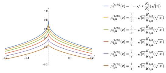
Figure 2.2: A Mathematica plot of the drift coefficients $\mu^{\beta{\downarrow}}_{\alpha}$ in (2.28) for various values of $\alpha$ and $\beta=1/2$ — the plot for $\mu^{(1/2){\downarrow}}_{0}(x)$ illustrates a very sharp cusp so that the value at $x=0$ should be understood as $1$.

For the second step (Section 6), we focus on the convergences of the Feynman–Kac semigroups in (2.10) and their extensions ${\mathbb{E}}^{(-\alpha)}_{z_{0}}[{\mathrm{e}}^{\Lambda_{\alpha}L_{t}}f(Z_{t})]$ as $\alpha\searrow 0$. The argument does not use ${\rm BES}(-\alpha,\beta{\downarrow})$ and essentially only operates at the expectation level.

The method of proof of Theorem 6.2 is what we emphasize, for it should be of independent interest for generalizations to other models of contact interaction. It provides a new, probabilistic construction of two-dimensional delta potentials by approximations of local times from lower-dimensional Bessel processes. In this direction, the following proposition illustrates the usefulness by showing an exact formula for the Laplace transform of ${\mathbb{E}}^{(-\alpha)}_{z_{0}}[{\mathrm{e}}^{\Lambda_{\alpha}L_{t}}f(Z_{t})]$. This contrasts the much more implicit formulas in [10, Proposition 2.1] under (1.8) and [1, (2.43)] under an operator form.

Proposition 2.9.

For all $\alpha\in(0,1/2)$, $\beta\in(0,\infty)$, $\lambda\in(\beta,\infty)$, $f\in\mathscr{B}_{+}(\mathbb{C})$ and $z_{0}\in\mathbb{C}$,

$$\begin{split}&\int_{0}^{\infty}{\mathrm{e}}^{-\lambda t}{\mathbb{E}}^{(-\alpha)}_{z_{0}}[{\mathrm{e}}^{\Lambda_{\alpha}L_{t}}f(Z_{t})]{\mathrm{d}}t\\ &{\quad\;}=U^{(-\alpha)}_{\lambda}f(z_{0})+\widehat{K}_{\alpha}(\sqrt{2\lambda}\lvert z_{0}\rvert)\cdot\frac{\frac{2^{1-\alpha}}{\Gamma(\alpha)}\cdot\beta^{\alpha}}{\lambda^{\alpha}-\beta^{\alpha}}\cdot U^{(-\alpha)}_{\lambda}f(0),\end{split}$$ (2.32)

where $\Lambda_{\alpha}=\Lambda_{\alpha}(\beta)$, $\widehat{K}_{\alpha}$ is defined in (2.4), and

$$U_{\lambda}^{(-\alpha)}f(z)\,{\stackrel{{\scriptstyle\rm def}}{{=}}}\int_{0}^{\infty}{\mathrm{e}}^{-\lambda t}{\mathbb{E}}^{(-\alpha)}_{z}[f(Z_{t})]{\mathrm{d}}t.$$ (2.33)

Moreover, $U^{(-\alpha)}_{\lambda}f(0)=\int_{0}^{\infty}{\mathbb{E}}_{0}^{(-\alpha)}[\overline{f}(\rho_{t})]{\mathrm{d}}t$, where $\overline{f}$ denotes the radialization of $f$:

$$\overline{f}(r)\,{\stackrel{{\scriptstyle\rm def}}{{=}}}\,\frac{1}{2\pi}\int_{-\pi}^{\pi}f(r{\mathrm{e}}^{{\mathtt{i}}\theta}){\mathrm{d}}\theta.$$ (2.34)

See (7.17) for the transition densities of ${\rm BES}(-\alpha)$.

Proof. To get (2.32), combine (LABEL:Lap:asymp), (6.30) and (6.35). See (6.16) for the definition of $F_{\alpha}$. Also, the alternative form of $U^{(-\alpha)}_{\lambda}f(0)$ by ${\rm BES}(-\alpha)$ restates Erickson’s characterization of this resolvent [22, (2.3) on p.75], for the case of $\{Z_{t}\}$ under ${\mathbb{P}}^{(-\alpha)}$. $\blacksquare$

3 No non-singular Feynman–Kac formulas exist

In this section, we fix $\beta\in(0,\infty)$ and prove Corollary 2.6. The following lemma extends (2.22) by using the standard Markovian type iteration.

Lemma 3.1.

Under Hypothesis 2.5, it holds that

$$\begin{split}&{\mathbb{E}}_{z_{0}}^{\mathbb{Q}}[{\mathrm{e}}^{A_{t}}\Phi_{t};\zeta>t]={\mathbb{E}}_{z_{0}}^{(0),\beta{\downarrow}}\left[D^{z_{0}}_{t}\Phi_{t}\right],\\ &\hskip 56.9055pt\forall\;z_{0}\in\mathbb{C}\setminus\{0\},\;t\in(0,\infty),\;\Phi\in\mathscr{B}_{+}(C([0,t],\mathbb{C})),\end{split}$$ (3.1)

where $\Phi_{t}$ is a shorthand notation for $\Phi(Z_{r};r\leq t)$.

Proof. Since the Borel $\sigma$-field on $C({\mathbb{R}}_{+},\mathbb{C})$ is generated by finite-dimensional measurable cylinder sets, (3.1) is implied by the particular case where for all integers $n\geq 1$,

$$\begin{split}&{\mathbb{E}}_{z_{0}}^{\mathbb{Q}}\Bigg{[}{\mathrm{e}}^{A_{t}}\prod_{j=1}^{n}\phi_{j}(Z_{r_{j}});\zeta>t\Bigg{]}={\mathbb{E}}_{z_{0}}^{(0),\beta{\downarrow}}\Bigg{[}D^{z_{0}}_{t}\prod_{j=1}^{n}\phi_{j}(Z_{r_{j}})\Bigg{]},\\ &\hskip 28.45274pt\forall\;z_{0}\in\mathbb{C}\setminus\{0\},\;t\in(0,\infty),\;\phi_{1},\cdots,\phi_{n}\in\mathscr{B}_{+}(\mathbb{C}),\;0<r_{1}<\cdots<r_{n}=t.\end{split}$$ (3.2)

To prove (3.2), we proceed with an induction on $n$. The case $n=1$ follows readily from (2.22) in the standing hypothesis. Next, assume that (3.2) holds for some integer $n-1$ such that $n-1\geq 1$. Then the conditions imposed in Hypothesis 2.5 imply

$${\quad\;}{\mathbb{E}}_{z_{0}}^{\mathbb{Q}}\Bigg{[}{\mathrm{e}}^{A_{t}}\prod_{j=1}^{n}\phi_{j}(Z_{r_{j}});\zeta>t\Bigg{]}$$

$$={\mathbb{E}}^{\mathbb{Q}}_{z_{0}}\Bigg{[}{\mathrm{e}}^{A_{r_{n-1}}}\prod_{j=1}^{n-1}\phi_{j}(Z_{r_{j}}){\mathbb{E}}^{\mathbb{Q}}_{Z_{r_{n-1}}}[{\mathrm{e}}^{A_{t-r_{n-1}}}\phi_{n}(Z_{t-r_{n-1}});\zeta>t-r_{n-1}];\zeta>r_{n-1}\Bigg{]}$$

$$={\mathbb{E}}^{\mathbb{Q}}_{z_{0}}\Bigg{[}{\mathrm{e}}^{A_{r_{n-1}}}\prod_{j=1}^{n-1}\phi_{j}(Z_{r_{j}}){\mathbb{E}}_{z}^{(0),\beta{\downarrow}}\big{[}D^{z}_{t-r_{n-1}}\phi_{n}(Z_{t-r_{n-1}})\big{]}\big{\rvert}_{z=Z_{r_{n-1}}};\zeta>r_{n-1}\Bigg{]}.$$ (3.3)

Note that in the second equality, it suffices to consider nonzero $z$ so that (2.22) applies. This restriction is enough because (2.4) implies

$${\mathbb{E}}^{\mathbb{Q}}_{z_{0}}[{\mathrm{e}}^{A_{t}}\mathds{1}_{\{0\}}(Z_{t});\zeta>t]={\mathbb{E}}_{z_{0}}^{(0),\beta{\downarrow}}\left[D^{z_{0}}_{t}\mathds{1}_{\{0\}}(Z_{t})\right]=0,\quad\forall\;z_{0}\in\mathbb{C}\setminus\{0\},\;t\in(0,\infty).$$

Now, the right-hand side of (3.3) takes the form of ${\mathbb{E}}^{\mathbb{Q}}_{z_{0}}[{\mathrm{e}}^{A_{r_{n-1}}}\prod_{j=1}^{n-1}\tilde{\phi}_{j}(Z_{r_{j}})]$. Since (3.1) is assumed to hold for $n-1$, (3.3) can be written as

$${\quad\;}{\mathbb{E}}_{z_{0}}^{\mathbb{Q}}\Bigg{[}{\mathrm{e}}^{A_{t}}\prod_{j=1}^{n}\phi_{j}(Z_{r_{j}});\zeta>t\Bigg{]}$$

$$={\mathbb{E}}^{(0),\beta{\downarrow}}_{z_{0}}\Bigg{[}D^{z_{0}}_{r_{n-1}}\prod_{j=1}^{n-1}\phi_{j}(Z_{r_{j}}){\mathbb{E}}_{z}^{(0),\beta{\downarrow}}\big{[}D^{z}_{t-r_{n-1}}\phi_{n}(Z_{t-r_{n-1}})\big{]}\big{\rvert}_{z=Z_{r_{n-1}}}\Bigg{]}$$

$$={\mathbb{E}}^{(0),\beta{\downarrow}}_{z_{0}}\Bigg{[}D^{z_{0}}_{t}\prod_{j=1}^{n}\phi_{j}(Z_{r_{j}})\Bigg{]}$$

by the Markov property of $\{Z_{t}\}$ under ${\mathbb{P}}^{(0),\beta{\downarrow}}$ and the multiplicativity of $D_{t}^{z}$. Recall (2.23). This establishes (3.2) for $n$, and hence, for all integers $n\geq 1$ by the induction hypothesis. We have proved (3.1). $\blacksquare$

Proof of Corollary 2.6.  We prove a contradiction to the existence of $(\mathbb{Q},A,\zeta)$. The crucial fact we apply below is that every nonnegative càdlàg supermartingale $\{N_{t}\}$ vanishes at all finite times $t\geq\inf\{s\geq 0;N_{s}=0\}\wedge\inf\{s\geq 0;N_{s-}=0\}$. See [39, Proposition 3.4 on p.70]. In the following argument, we fix $z_{0}\in\mathbb{C}\setminus\{0\}$.

Step 1. In this step, we show that the existence of $(\mathbb{Q},A,\zeta)$ implies

$${\mathbb{E}}_{z_{0}}^{(0),\beta{\downarrow}}\left[\left.{\mathbb{E}}^{(0),\beta{\downarrow}}_{0}\left[\frac{1}{K_{0}(\sqrt{2\beta}\lvert Z_{t-s}\rvert)}\right]\right\rvert_{s=T_{0}(Z)};t\geq T_{0}(Z)\right]=0,\quad\forall\;t\in(0,\infty).$$ (3.4)

To see (3.4), first we apply the fact for supermartingales just recalled to the process $M^{z_{0}}_{t}\,{\stackrel{{\scriptstyle\rm def}}{{=}}}\,{\mathrm{e}}^{-A_{t}}D^{z_{0}}_{t}$. This is indeed a ${\mathbb{P}}^{(0),\beta{\downarrow}}_{z_{0}}$-supermartingale, since for all nonnegative $\Phi$ and $s,t\in(0,\infty)$, (3.1) gives

$${\mathbb{E}}_{z_{0}}^{(0),\beta{\downarrow}}\left[M^{z_{0}}_{t+s}\Phi_{t}\right]={\mathbb{E}}_{z_{0}}^{\mathbb{Q}}[\Phi_{t};\zeta>t+s]\leq{\mathbb{E}}_{z_{0}}^{\mathbb{Q}}[\Phi_{t};\zeta>t]={\mathbb{E}}_{z_{0}}^{(0),\beta{\downarrow}}\left[M^{z_{0}}_{t}\Phi_{t}\right].$$

Then it follows from the supermartingale property that

$${\mathbb{E}}_{z_{0}}^{(0),\beta{\downarrow}}\left[M^{z_{0}}_{t}\Phi_{t}\right]={\mathbb{E}}_{z_{0}}^{(0),\beta{\downarrow}}\left[M^{z_{0}}_{t}\Phi_{t};t<T_{0}(M^{z_{0}})\right].$$

Furthermore, by the definition of $\{M^{z_{0}}_{t}\}$, the foregoing identity implies

$${\mathbb{E}}_{z_{0}}^{(0),\beta{\downarrow}}\left[\frac{1}{K_{0}(\sqrt{2\beta}\lvert Z_{t}\rvert)}\right]={\mathbb{E}}_{z_{0}}^{(0),\beta{\downarrow}}\left[\frac{1}{K_{0}(\sqrt{2\beta}\lvert Z_{t}\rvert)};t<T_{0}(Z)\right],$$

which uses the non-singular assumption that ${\mathrm{e}}^{A_{t}(\mathrm{w}_{r};r\leq t)}$ does not vanish so that the identities $T_{0}(M^{z_{0}})=T_{0}(D^{z_{0}})=T_{0}(Z)$ hold. Hence, we must have

$$0 ={\mathbb{E}}_{z_{0}}^{(0),\beta{\downarrow}}\left[\frac{1}{K_{0}(\sqrt{2\beta}\lvert Z_{t}\rvert)};t\geq T_{0}(Z)\right]$$

$$={\mathbb{E}}_{z_{0}}^{(0),\beta{\downarrow}}\left[\left.{\mathbb{E}}^{(0),\beta{\downarrow}}_{0}\left[\frac{1}{K_{0}(\sqrt{2\beta}\lvert Z_{t-s}\rvert)}\right]\right\rvert_{s=T_{0}(Z)};t\geq T_{0}(Z)\right]$$

by the strong Markov property of $\{Z_{t}\}$ at $T_{0}(Z)$ under ${\mathbb{P}}^{(0),\beta{\downarrow}}_{z_{0}}$. (Recall that this strong Markov property holds under ${\rm BES}(0,\beta{\downarrow})$ and is extended to $\{Z_{t}\}$ under ${\mathbb{P}}^{(0),\beta{\downarrow}}_{z_{0}}$ thanks to Erickson’s theorem [22, Theorem 1].) The last equality proves (3.4).

Step 2. Now, (3.4) leads to the required contradiction since its left-hand side is actually strictly positive by the following two properties:

1. The stopping time $T_{0}(Z)=T_{0}(\lvert Z\rvert)$ under ${\mathbb{P}}^{(0),\beta{\downarrow}}_{z_{0}}$ is distributed as the generalized inverse Gaussian distribution ${\rm GIG}(0;\lvert z_{0}\rvert,\sqrt{2\beta})$ [20, p.884]:

   $${\mathbb{P}}^{(0),\beta{\downarrow}}_{z_{0}}(T_{0}(Z)\in{\mathrm{d}}t)=\frac{1}{2K_{0}(\sqrt{2\beta}\lvert z_{0}\rvert)}\exp\left(-\beta t-\frac{\lvert z_{0}\rvert^{2}}{2t}\right){\mathrm{d}}t,\quad t\in(0,\infty).$$ (3.5)

   Hence, $T_{0}(Z)$ has a continuous, everywhere strictly positive density on $(0,\infty)$. See also (4.2).

2. For all $t\in(0,\infty)$, ${\mathbb{E}}^{(0),\beta{\downarrow}}_{0}[K_{0}(\sqrt{2\beta}\lvert Z_{t}\rvert)^{-1}]>0$ by (2.4).

The proof of Corollary 2.6 is complete. $\blacksquare$

4 Excursions of the inter-particle distance

In this section, we give the first proof of Theorem 2.4 by applying the original characterization of ${\rm BES}(0,\beta{\downarrow})$ in [20] by excursion theory. The reader may consult [7, Chapter IV] and [9] for the excursion theory of general Markov processes.

As before, let $\{\rho_{t}\}$ under ${\mathbb{P}}^{(0),\beta{\downarrow}}$ denote a version of ${\rm BES}(0,\beta{\downarrow})$. Then the probability law of $\{\rho_{t};t<T_{0}(\rho)\}$ can be characterized as follows:

$$\begin{split}{\mathbb{P}}^{(0),\beta{\downarrow}}_{x_{0}}(\{t<T_{0}\}\cap A)&={\mathbb{E}}^{(0)}_{x_{0}}\left[\frac{{\mathrm{e}}^{-\beta t}K_{0}(\sqrt{2\beta}\rho_{t})}{K_{0}(\sqrt{2\beta}x_{0})};A\right],\\ &\quad\quad\forall\;A\in\sigma(\rho_{s};s\leq t),\;x_{0}\in(0,\infty).\end{split}$$ (4.1)

In particular, we deduce that

$${\mathbb{E}}^{(0),\beta{\downarrow}}_{x_{0}}[{\mathrm{e}}^{-qT_{0}(\rho)}]=\frac{K_{0}(\sqrt{2(\beta+q)}x_{0})}{K_{0}(\sqrt{2\beta}x_{0})},\quad\forall\;q,x_{0}\in(0,\infty).$$ (4.2)

See [20, (2.4) and (2.9) on pp.883–884] for (4.1) and (4.2).

The description of $\{\rho_{t}\}$ after $T_{0}(\rho)$ is via a choice of local time and excursion measure at $0$, denoted by $\{L_{t}\}$ and $\mathbf{N}^{\beta{\downarrow}}_{0}$, respectively, such that the following holds:

$${\mathbb{E}}^{(0),\beta{\downarrow}}_{0}\left[\int_{0}^{\infty}{\mathrm{e}}^{-qt}{\mathrm{d}}L_{t}\right]=\frac{1}{\log(1+q/\beta)},\quad\forall\;q\in(0,\infty),$$ (4.3)

and, with $\zeta(\epsilon)$ denoting the lifetime of a generic excursion $\epsilon=\{\epsilon_{t}\}$,

1. $\mathbf{N}_{0}^{\beta{\downarrow}}(\zeta(\epsilon)\in{\mathrm{d}}v)=v^{-1}{\mathrm{e}}^{-\beta v}{\mathrm{d}}v$, and

2. conditioned on $\zeta=v$, $\{\epsilon_{t};0\leq t\leq v\}$ is a two-dimensional Bessel bridge from $0$ to $0$ over $[0,v]$.

See [20, Theorem 2.1 and Corollary 2.3 on pp.883–884] for (4.3), (i) and (ii). Standard properties of Bessel bridges can be found in [39, Section XI.3 on pp.463+]. To use (ii), note that for all $t\in(0,v)$, the explicit probability densities of ${\rm BES}(0)$ in (7.17) give

$$\mathbf{N}^{\beta{\downarrow}}_{0}(\epsilon_{t}\in{\mathrm{d}}y\mid\zeta(\epsilon)=v) =\lim_{y_{0}\searrow 0}\frac{p^{(0)}_{t}(0,y)p^{(0)}_{v-t}(y,y_{0})}{p^{(0)}_{v}(0,y_{0})}$$

$$=\lim_{y_{0}\searrow 0}\frac{\frac{y}{t}\exp(-\frac{y^{2}}{2t})\frac{y_{0}}{v-t}\exp(-\frac{y^{2}+y_{0}^{2}}{2(v-t)})I_{0}(\frac{yy_{0}}{v-t})}{\frac{y_{0}}{v}\exp(-\frac{y_{0}^{2}}{2v})}$$

$$=\frac{vy}{t(v-t)}\exp\left(-\frac{y^{2}}{2t}-\frac{y^{2}}{2(v-t)}\right),$$ (4.4)

where the last equality follows since the modified Bessel function of the first kind $I_{0}(y_{1})$ is asymptotically equal to $1$ as $y_{1}\searrow 0$. See (7.19) for this representation.

First proof of Theorem 2.4.  We only prove (2.18) and (2.19) below. The proof of (2.4) follows immediately from (2.18) and (2.19).

To prove (2.18), fix $f\in\mathscr{B}_{+}(\mathbb{C})$ and $z_{0}\in\mathbb{C}\setminus\{0\}$, and write

$${\quad\;}{\mathbb{E}}_{z_{0}}^{(0),\beta{\downarrow}}\left[\frac{{\mathrm{e}}^{\beta t}K_{0}(\sqrt{2\beta}\lvert z_{0}\rvert)}{K_{0}(\sqrt{2\beta}\lvert Z_{t}\rvert)}f(Z_{t})\right]$$

$$={\mathbb{E}}_{z_{0}}^{(0),\beta{\downarrow}}\left[\frac{{\mathrm{e}}^{\beta t}K_{0}(\sqrt{2\beta}\lvert z_{0}\rvert)}{K_{0}(\sqrt{2\beta}\lvert Z_{t}\rvert)}f(Z_{t});t<T_{0}(Z)\right]+{\mathbb{E}}^{(0),\beta{\downarrow}}_{z_{0}}\left[\frac{{\mathrm{e}}^{\beta t}K_{0}(\sqrt{2\beta}\lvert z_{0}\rvert)}{K_{0}(\sqrt{2\beta}\lvert Z_{t}\rvert)}f(Z_{t});t\geq T_{0}(Z)\right]$$

$$={\mathbb{E}}^{(0)}_{z_{0}}\left[f(Z_{t})\right]+{\mathbb{E}}^{(0),\beta{\downarrow}}_{z_{0}}\left[\frac{{\mathrm{e}}^{\beta t}K_{0}(\sqrt{2\beta}\lvert z_{0}\rvert)}{K_{0}(\sqrt{2\beta}\lvert Z_{t}\rvert)}f(Z_{t});t\geq T_{0}(Z)\right].$$ (4.5)

To justify the first term in the last equality, recall that by (2.13), $\{Z_{t}\}$ before $T_{0}(Z)=T_{0}(\rho)$ has the same skew-product representation as planar Brownian motion, and then we use (4.1) and the independence $\{\lvert Z_{t}\rvert\}{\perp\!\!\!\perp}\{\gamma_{t}\}$.

To evaluate the last expectation in (4.5), recall the radialization of $f$ defined by (2.34). Then the Laplace transform of that expectation satisfies, for all $\lambda\in(\beta,\infty)$,

$$\quad\int_{0}^{\infty}{\mathrm{e}}^{-\lambda t}{\mathbb{E}}^{(0),\beta{\downarrow}}_{z_{0}}\left[\frac{{\mathrm{e}}^{\beta t}K_{0}(\sqrt{2\beta}\lvert z_{0}\rvert)}{K_{0}(\sqrt{2\beta}\lvert Z_{t}\rvert)}f(Z_{t});t\geq T_{0}(Z)\right]{\mathrm{d}}t$$

$$={\mathbb{E}}^{(0),\beta{\downarrow}}_{z_{0}}[{\mathrm{e}}^{-(\lambda-\beta)T_{0}(Z)}]\cdot\int_{0}^{\infty}{\mathrm{e}}^{-(\lambda-\beta)t}{\mathbb{E}}^{(0),\beta{\downarrow}}_{0}\left[\frac{K_{0}(\sqrt{2\beta}\lvert z_{0}\rvert)}{K_{0}(\sqrt{2\beta}\lvert Z_{t}\rvert)}\overline{f}(\lvert Z_{t}\rvert)\right]{\mathrm{d}}t$$ (4.6)

by the strong Markov property of $\{Z_{t}\}$ at time $T_{0}(Z)$ and Erickson’s characterization of the resolvent of $\{Z_{t}\}$ at the origin [22, (2.3) on p.75]. The last equality now allows for an application of the other descriptions of ${\rm BES}(0,\beta{\downarrow})$ recalled above. By (4.2), (4.3), and the compensation formula in excursion theory [7, (7) on p.120], we have

$$\quad\int_{0}^{\infty}{\mathrm{e}}^{-\lambda t}{\mathbb{E}}^{(0),\beta{\downarrow}}_{z_{0}}\left[\frac{{\mathrm{e}}^{\beta t}K_{0}(\sqrt{2\beta}\lvert z_{0}\rvert)}{K_{0}(\sqrt{2\beta}\lvert Z_{t}\rvert)}f(Z_{t});t\geq T_{0}(Z)\right]{\mathrm{d}}t$$

$$=\frac{K_{0}(\sqrt{2\lambda}\lvert z_{0}\rvert)}{K_{0}(\sqrt{2\beta}\lvert z_{0}\rvert)}\cdot\frac{1}{\log[1+(\lambda-\beta)/\beta]}\mathbf{N}_{0}^{\beta{\downarrow}}\left(\int_{0}^{\zeta}{\mathrm{e}}^{-(\lambda-\beta)t}\frac{K_{0}(\sqrt{2\beta}\lvert z_{0}\rvert)}{K_{0}(\sqrt{2\beta}\epsilon_{t})}\overline{f}(\epsilon_{t}){\mathrm{d}}t\right)$$ (4.7)

$$=\frac{\pi}{\log(\lambda/\beta)}\left(\int_{0}^{\infty}{\mathrm{e}}^{-\lambda t}P_{t}(z_{0}){\mathrm{d}}t\right)\mathbf{N}_{0}^{\beta{\downarrow}}\left(\int_{0}^{\zeta}{\mathrm{e}}^{-(\lambda-\beta)t}\frac{\overline{f}(\epsilon_{t})}{K_{0}(\sqrt{2\beta}\epsilon_{t})}{\mathrm{d}}t\right),$$ (4.8)

where the last equality holds since (2.5) implies

$$\int_{0}^{\infty}{\mathrm{e}}^{-\lambda t}P_{t}(z){\mathrm{d}}t=\frac{1}{\pi}K_{0}(\sqrt{2\lambda}\lvert z\rvert).$$ (4.9)

Next, we compute for an explicit form of the $\mathbf{N}^{\beta{\downarrow}}_{0}$-expectation in (4.8). By the description of $\mathbf{N}^{\beta{\downarrow}}_{0}$ stated below (4.3) and by (4.4), it holds that for all nonnegative $g$,

$${\quad\;}\mathbf{N}^{\beta{\downarrow}}_{0}\left(\int_{0}^{\zeta}{\mathrm{e}}^{-(\lambda-\beta)t}g(\epsilon_{t}){\mathrm{d}}t\right)$$

$$=\int_{0}^{\infty}\frac{{\mathrm{e}}^{-\beta v}}{v}\int_{0}^{v}{\mathrm{e}}^{-(\lambda-\beta)t}\int_{0}^{\infty}\frac{vy}{t(v-t)}\exp\left(-\frac{y^{2}}{2t}-\frac{y^{2}}{2(v-t)}\right)g(y){\mathrm{d}}y{\mathrm{d}}t{\mathrm{d}}v$$

$$=\int_{0}^{\infty}{\mathrm{e}}^{-\lambda t}\int_{0}^{\infty}\frac{1}{t}\exp\left(-\frac{y^{2}}{2t}\right)yg(y)\int_{t}^{\infty}{\mathrm{e}}^{-\beta(v-t)}\frac{1}{(v-t)}\exp\left(-\frac{y^{2}}{2(v-t)}\right){\mathrm{d}}v{\mathrm{d}}y{\mathrm{d}}t$$

$$=\int_{0}^{\infty}{\mathrm{e}}^{-\lambda t}\int_{0}^{\infty}\frac{1}{t}\exp\left(-\frac{y^{2}}{2t}\right)yg(y)\cdot 2K_{0}(\sqrt{2\beta}y){\mathrm{d}}y{\mathrm{d}}t,$$

where the last equality uses (2.5) for $\nu=0$ after a change of variable that replaces $\beta(v-t)$ with $v$. Hence, by the polar coordinates and the definition (2.34) of $\bar{f}$, we get

$$\mathbf{N}^{\beta{\downarrow}}_{0}\left(\int_{0}^{\zeta}{\mathrm{e}}^{-(\lambda-\beta)t}\frac{\overline{f}(\epsilon_{t})}{K_{0}(\sqrt{2\beta}\epsilon_{t})}{\mathrm{d}}t\right)=2\int_{0}^{\infty}{\mathrm{e}}^{-\lambda t}P_{t}f(0){\mathrm{d}}t.$$ (4.10)

Now, combining (4.5), (4.8) and (4.10), we get

$$\quad\int_{0}^{\infty}{\mathrm{e}}^{-\lambda t}{\mathbb{E}}^{(0),\beta{\downarrow}}_{z_{0}}\left[\frac{{\mathrm{e}}^{\beta t}K_{0}(\sqrt{2\beta}\lvert z_{0}\rvert)}{K_{0}(\sqrt{2\beta}\lvert Z_{t}\rvert)}f(Z_{t})\right]{\mathrm{d}}t$$

$$=\int_{0}^{\infty}{\mathrm{e}}^{-\lambda t}P_{t}f(z_{0}){\mathrm{d}}t+\frac{2\pi}{\log(\lambda/\beta)}\left(\int_{0}^{\infty}{\mathrm{e}}^{-\lambda t}P_{t}(z_{0}){\mathrm{d}}t\right)\left(\int_{0}^{\infty}{\mathrm{e}}^{-\lambda t}P_{t}f(0){\mathrm{d}}t\right).$$ (4.11)

To match the right-hand side of (4.11) with the Laplace transform of $\{P^{\beta}_{t}\}$ in (1.4), note that

$$P_{t}f(z)={\mathbb{E}}^{(0)}_{{\sqrt{2}}z}[f(Z_{2t}/{\sqrt{2}})]=P_{2t}\{\tilde{z}\mapsto f(\tilde{z}/{\sqrt{2}})\}({\sqrt{2}}z),\quad P_{t}(z)=2P_{2t}({\sqrt{2}}z).$$ (4.12)

Also, recall that the inversion of the Laplace transform formula in (1.4) is given by (2.15). Hence, we get (2.18) upon applying (4.12) to (4.11).

The proof of (2.19) is similar. Now, as in (4.7), we obtain from (4.3) and the compensation formula in excursion theory [7, (7) on p.120] that

$$\int_{0}^{\infty}{\mathrm{e}}^{-\lambda t}{\mathbb{E}}^{(0),\beta{\downarrow}}_{0}\left[\frac{{\mathrm{e}}^{\beta t}\cdot 2\pi}{K_{0}(\sqrt{2\beta}\lvert Z_{t}\rvert)}f(Z_{t})\right]{\mathrm{d}}t =\frac{2\pi}{\log(\lambda/\beta)}\mathbf{N}^{\beta{\downarrow}}_{0}\left(\int_{0}^{\zeta}{\mathrm{e}}^{-(\lambda-\beta)t}\frac{\bar{f}(\epsilon_{t})}{K_{0}(\sqrt{2\beta}\epsilon_{t})}{\mathrm{d}}t\right)$$

$$=\frac{4\pi}{\log(\lambda/\beta)}\left(\int_{0}^{\infty}{\mathrm{e}}^{-\lambda t}P_{t}f(0){\mathrm{d}}t\right)$$

by (4.10). Hence, by the first equality in (4.12), we get

$$\int_{0}^{\infty}{\mathrm{e}}^{-\lambda t}{\mathbb{E}}^{(0),\beta{\downarrow}}_{0}\left[\frac{{\mathrm{e}}^{\beta t}\cdot 2\pi}{K_{0}(\sqrt{\beta}\lvert{\sqrt{2}}Z_{t}\rvert)}f({\sqrt{2}}Z_{t})\right] =\frac{4\pi}{\log(\lambda/\beta)}\left(\int_{0}^{\infty}{\mathrm{e}}^{-\lambda t}P_{2t}f(0){\mathrm{d}}t\right)$$

$$=\int_{0}^{\infty}{\mathrm{e}}^{-\lambda t}\mathring{P}^{\beta}_{t}f{\mathrm{d}}t,$$

where the last equality can be seen by comparing (1.4) and (2.15) or by the proof of [10, Proposition 5.1]. The last equality proves (2.19). The proof is complete. $\blacksquare$

5 SDEs for the inter-particle distance

In this section, we start the second proof of Theorem 2.4 by studying the SDE satisfied by ${\rm BES}(-\alpha,\beta{\downarrow})$ for $\alpha\in[0,1/2)$; the remaining of this proof appears in Section 6. Our main goal in this section is to prove Theorem 2.8. In particular, ${\rm BES}(0,\beta{\downarrow})$ will be identified as the $(\alpha\searrow 0)$-distributional limit of ${\rm BES}(-\alpha,\beta{\downarrow})$ as in [20].

5.1 Comparison of solutions and strong well-posedness

We first prove Theorem 2.8 (1^∘), leaving the proofs of Theorem 2.8 (2^∘), (3^∘) and (4^∘) to Section 5.2 and 5.3. Let us begin with some observations for the coefficient $\mu^{\beta{\downarrow}}_{\alpha}$ in (2.29). First, the discussion below (5.62) shows that the continuity of $\mu^{\beta{\downarrow}}_{\alpha}(x)$ at $x=0$ holds with $\mu^{\beta{\downarrow}}_{\alpha}(0)=2(1-\alpha)$, so $\mu^{\beta{\downarrow}}_{\alpha}$ defines a continuous function. The continuity at $x=0$ is nonetheless ill-behaved: For $\alpha\in(0,1/2)$, $\mu^{\beta{\downarrow}}_{\alpha}(x)$ is Hölder-$\alpha$ at $x=0$. For $\alpha=0$, $\mu^{\beta{\downarrow}}_{\alpha}(x)$ is not even Hölder continuous: $\mu^{\beta{\downarrow}}_{0}(x)-2\sim 2/\log\sqrt{2\beta\lvert x\rvert}$ as $\lvert x\rvert\to 0$. Recall Figure 2.2.

For the following proof of comparison of solutions and pathwise uniqueness, the ill-behaved continuity of the drift coefficients just pointed out makes the standard theorems not directly applicable. We are neither aware of any existing general methods that can apply for all $\alpha\in[0,1/2)$. On the other hand, the following proof deals with all of these cases and proceeds with the alternative expression of $\mu^{\beta{\downarrow}}_{\alpha}(x)$ given by

$$\mu^{\beta{\downarrow}}_{\alpha}(x)=2-2R_{\alpha}(\sqrt{2\beta\lvert x\rvert}).$$ (5.1)

See (5.62) for the precise definition of $R_{\alpha}$. Several key properties of $R_{\alpha}$ applied in the proof will be shown separately in Section 5.4.

Proposition 5.1.

Fix $\beta\in(0,\infty)$.

1. For all $\alpha\in[0,1/2)$ and $x_{0}\geq 0$, the solutions to (2.28) are nonnegative.

2. Fix $\alpha_{1},\alpha_{2}\in[0,1/2)$ with $\alpha_{1}<\alpha_{2}$, and $x_{1},x_{2}\in{\mathbb{R}}_{+}$ with $x_{1}\geq x_{2}$. Any two solutions to (2.28) with $(x_{0},\alpha)=(x_{1},\alpha_{1})$ and $(x_{0},\alpha)=(x_{2},\alpha_{2})$, denoted by $X_{\alpha_{1}}(t)$ and $X_{\alpha_{2}}(t)$, respectively, satisfy ${\mathbb{P}}(X_{\alpha_{1}}(t)\geq X_{\alpha_{2}}(t),\,\forall\;t\in{\mathbb{R}}_{+})=1$.

3. For all $\alpha\in[0,1/2)$ and $x_{0}\geq 0$, there is pathwise uniqueness in (2.28).

Proof. (1^∘) We compare (2.28) with the following strongly well-posed SDE:

$$Y_{t}=x_{0}^{2}-\int_{0}^{t}4\beta Y_{s}{\mathrm{d}}s+2\int_{0}^{t}\lvert Y_{s}\rvert^{1/2}{\mathrm{d}}\widetilde{W}_{s}.$$ (5.2)

First, to see the strong well-posedness of (5.2), note that the weak existence of solutions holds since the drift and noise coefficients are continuous and have at most linear growth [26, Theorems 2.3 and 2.4 on p.159 and p.163]. The pathwise uniqueness holds by [30, 2.13 Proposition on p.291]. Hence, [30, 3.23 Corollary on p.310] applies and reinforces the weak existence to the strong existence.

Now, we apply the comparison theorem of SDEs [30, 2.18 Proposition on p.293] to get $X_{t}\geq Y_{t}$ for all $t$ with probability one. This comparison is legitimate since, by Corollary 5.9, the drift coefficient of (2.28) dominates the drift coefficient of (5.2) everywhere, and the latter drift coefficient is Lipschitz. Also, $Y_{t}\geq 0$ for all $t$ with probability one by the same comparison theorem of SDEs since the drift coefficient in (5.2) is Lipschitz and the solution to (5.2) for $x_{0}=0$ is the zero process. The required nonnegativity of solutions to (2.28) follows.

(2^∘) Since $\mu^{\beta{\downarrow}}_{\alpha}(x)$ is strictly decreasing in $\alpha$ for all fixed $x$ by (5.1) and Proposition 5.8 (2^∘), another comparison theorem of SDEs [30, 2.19 Exercise on p.294] applies and gives the required result.

(3^∘) Let us begin by reducing the problem of pathwise uniqueness to the problem of uniqueness in law. Given any two solutions $X,\widetilde{X}$ to (2.28), the square-root noise coefficient implies that $X-\widetilde{X}$ has zero semimartingale local time at level $0$ [39, (3.4) Corollary on p.390]. Therefore, by [39, (3.2) Proposition on p.389], for any $\alpha\in[0,1/2)$ and $x_{0}\geq 0$, the uniqueness in law in (2.28) implies its pathwise uniqueness. Then thanks to Proposition 5.2 proven below, it remains to prove the uniqueness in law for any $\alpha\in(0,1/2)$ and $x_{0}\geq 0$. This is divided into two steps: Step 1 shows the uniqueness in law, assuming that any solution $\{X_{t}\}$ satisfies the following property:

$$\textstyle\int_{0}^{t}{\mathrm{d}}s/X_{s}^{1-2\alpha}<\infty,\quad\forall\;t\in(0,\infty).$$ (5.3)

Step 2 verifies (5.3) to complete the proof.

Step 1. Our main goal of this part is to show that under (5.3),

$${\mathbb{E}}[G(X_{t\wedge\tau_{n}};t\leq T)]={\mathbb{E}}^{(-\alpha),\beta{\downarrow}}_{x_{0}}[G(\rho^{2}_{t\wedge\tau_{n}^{\prime}};t\leq T)]$$ (5.4)

for all $n\in\mathbb{N}$, $T\in(0,\infty)$ and bounded continuous $G\in\mathscr{B}_{+}(C([0,T],{\mathbb{R}}_{+}))$, where

$$\tau_{n}\textstyle{\stackrel{{\scriptstyle\rm def}}{{=}}}\inf\{t\geq 0;\int_{0}^{t}{\mathrm{d}}s/X_{s}^{1-2\alpha}\geq n\},\quad\tau_{n}^{\prime}\textstyle{\stackrel{{\scriptstyle\rm def}}{{=}}}\inf\{t\geq 0;\int_{0}^{t}{\mathrm{d}}s/\rho_{s}^{2-4\alpha}\geq n\}.$$

Since $\tau_{n}\nearrow\infty$ by (5.3) and $\tau_{n}^{\prime}\nearrow\infty$ under ${\mathbb{P}}_{x_{0}}^{(-\alpha)}$ by Proposition 7.1 (2^∘), passing $n\to\infty$ on both sides of (5.4) proves that $\{X_{t};0\leq t\leq T\}$ has the same law as $\{\rho^{2}_{t};0\leq t\leq T\}$ under ${\mathbb{P}}^{(-\alpha),\beta{\downarrow}}_{x_{0}}$, and so, the required uniqueness in law under (5.3).

To prove (5.4), the informal idea is to postulate that $\{X_{t}\}$ arises from a change of measure as that for ${\rm BES}(-\alpha,\beta{\downarrow})$ by ${\rm BES}(-\alpha)$, so we aim to identify a version of ${\rm BES}(-\alpha)$ underlying the law of $\{X_{t}\}$. Recall that $\{N_{t}\}$ in (5.20) defines the exponential martingale to change measure from ${\rm BES}(-\alpha)$ to ${\rm BES}(-\alpha,\beta{\downarrow})$. Accordingly, we formulate an analogue of the reciprocal of this exponential martingale and define

$$\widetilde{N}_{t}\,{\stackrel{{\scriptstyle\rm def}}{{=}}}\,\sqrt{2\beta}\int_{0}^{t}\frac{K_{1-\alpha}}{K_{\alpha}}(\sqrt{2\beta X_{s}}){\mathrm{d}}\widetilde{W}_{s},$$ (5.5)

and consider a probability measure $\mathbb{Q}_{n,T}$ defined by

$${\mathrm{d}}\mathbb{Q}_{n,T}\,{\stackrel{{\scriptstyle\rm def}}{{=}}}\,\mathscr{E}(\widetilde{N})_{T\wedge\tau_{n}}{\mathrm{d}}{\mathbb{P}}.$$ (5.6)

Here, $\mathbb{Q}_{n,T}$ is indeed a probability measure since by (5.60), $\langle\widetilde{N},\widetilde{N}\rangle_{\tau_{n}}\leq C(\alpha,\beta,n)$, and so, by Novikov’s criterion [39, (1.15) Proposition on p.332], the exponential local martingale $\mathscr{E}(\widetilde{N})$ associated with $\{\widetilde{N}_{t}\}$ is a martingale under ${\mathbb{P}}$ if stopped at time $\tau_{n}$.

Next, we show how inverting the Girsanov transformation in (5.6) leads to (5.4). First, use (5.6) to get

$${\mathbb{E}}[F(X_{t\wedge\tau_{n}},\widetilde{W}_{t\wedge\tau_{n}};t\leq T)] ={\mathbb{E}}^{\mathbb{Q}_{n,T}}\left[\frac{F(X_{t\wedge\tau_{n}},\widetilde{W}_{t\wedge\tau_{n}};t\leq T)}{\mathscr{E}(\widetilde{N})_{T\wedge\tau_{n}}}\right]$$

$$={\mathbb{E}}^{\mathbb{Q}_{n,T}}[\mathscr{E}(N^{(n)})_{T\wedge\tau_{n}}F(X_{t\wedge\tau_{n}},\widetilde{W}_{t\wedge\tau_{n}};t\leq T)],$$ (5.7)

where in the last equality, we define

$$N^{(n)}_{t} \,{\stackrel{{\scriptstyle\rm def}}{{=}}}-\sqrt{2\beta}\int_{0}^{t}\frac{K_{1-\alpha}}{K_{\alpha}}(\sqrt{2\beta X_{s}}){\mathrm{d}}W^{(n)}_{s},$$

$$W^{(n)}_{t} \,{\stackrel{{\scriptstyle\rm def}}{{=}}}\,\widetilde{W}_{t}-\sqrt{2\beta}\int_{0}^{t}\frac{K_{1-\alpha}}{K_{\alpha}}(\sqrt{2\beta X_{s}}){\mathrm{d}}s.$$

By Girsanov’s theorem [39, (1.7) Theorem on p.329], $\{W^{(n)}_{t\wedge\tau_{n}};0\leq t\leq T\}$ under $\mathbb{Q}_{n,T}$ is a Brownian motion stopped at time $\tau_{n}$, and $\{X_{t\wedge\tau_{n}};0\leq t\leq T\}$ under $\mathbb{Q}_{n,T}$ obeys the SDE of ${\rm BES}Q(-\alpha)$ stopped at time $\tau_{n}$ and driven by $W_{\cdot\wedge\tau_{n}}^{(n)}$. Furthermore, notice that the last expectation in (5.7) can be written as an expectation of ${\rm BES}Q(-\alpha,\beta{\downarrow})$ and its driving Brownian motion: Taking $\{N_{t}\}$ as in Proposition 5.3, we deduce from the SDE dynamics of $\{X_{t\wedge\tau_{n}};0\leq t\leq T\}$ under $\mathbb{Q}_{n,T}$ mentioned above and the pathwise uniqueness in the SDE of ${\rm BES}Q(-\alpha)$ that

$${\mathbb{E}}^{\mathbb{Q}_{n,T}}[\mathscr{E}(N^{(n)})_{T\wedge\tau_{n}}F(X_{t\wedge\tau_{n}},\widetilde{W}_{t\wedge\tau_{n}};t\leq T)] ={\mathbb{E}}^{(-\alpha)}_{x_{0}}[\mathscr{E}(N)_{T\wedge\tau_{n}^{\prime}}F(\rho_{t\wedge\tau_{n}^{\prime}}^{2},\widetilde{W}_{t\wedge\tau_{n}^{\prime}};t\leq T)]$$

$$={\mathbb{E}}^{(-\alpha),\beta{\downarrow}}_{x_{0}}[F(\rho_{t\wedge\tau_{n}^{\prime}}^{2},\widetilde{W}_{t\wedge\tau_{n}^{\prime}};t\leq T)],$$ (5.8)

where $\widetilde{W}$ under ${\mathbb{P}}^{(-\alpha)}$ relates the driving Brownian motion $W$ of ${\rm BES}(-\alpha)$ as in (5.21), and the last equality follows from (2.3). Combining (5.7) and (5.8) gives (5.4).

Step 2. To verify (5.3), the informal idea is to compare $\{X_{t}\}$ with ${\rm BES}Q(-\alpha-\delta)$ whenever $\{X_{t}\}$ is nearly zero, where $\delta>0$ is small. To carry this out, choose $\delta\in(0,1)$ such that (i) $\alpha+\delta\in(0,1/2)$, and (ii) $\eta=-2+4\alpha\leq 0$ fulfills the condition of Proposition 7.1 (2^∘) with $\alpha$ there replaced by $\alpha+\delta$. Condition (ii) is equivalent to

$$1-2(\alpha+\delta)+(-2+4\alpha)>-1.$$ (5.9)

(We have no room to choose $\delta>0$ if $\alpha=0$.) Then with respect to $\delta$, the discussion below (5.62) allows a choice of $\gamma>0$ such that

$$\sup_{x\in(0,2\gamma]}\sqrt{2\beta x}\frac{K_{1-\alpha}}{K_{\alpha}}(\sqrt{2\beta x})<\frac{\delta}{2}.$$ (5.10)

Next, we choose subintervals of $[0,T]$ for the comparison, for any fixed $T\in(0,\infty)$:

$$\left.\begin{array}[]{ll}S_{1}{\stackrel{{\scriptstyle\rm def}}{{=}}}\inf\{t\geq 0;X_{t}\leq\gamma\}\wedge T,&T_{1}{\stackrel{{\scriptstyle\rm def}}{{=}}}\inf\{t>S_{1};X_{t}=2\gamma\}\wedge T,\\ S_{n+1}{\stackrel{{\scriptstyle\rm def}}{{=}}}\inf\{t>T_{n};X_{t}=\gamma\}\wedge T,&T_{n+1}{\stackrel{{\scriptstyle\rm def}}{{=}}}\inf\{t>S_{n+1};X_{t}=2\gamma\}\wedge T,\end{array}\right.$$ (5.13)

where the stopping times in the second line are defined for $n\in\mathbb{N}$ and inductively on $n$ starting with the stopping times in the first line. (Note that $S_{1}$ is defined with the weaker condition “$X_{t}\leq\gamma$” so that $S_{1}=0$ whenever $X_{0}\leq\gamma$.) Then

$$\{t\in[0,T];X_{t}\leq\gamma\}\subset\bigcup_{n=1}^{\infty}[S_{n},T_{n}],$$ (5.14)

$$\mu^{\beta{\downarrow}}_{\alpha}(X_{t})=2-2R_{\alpha}(\sqrt{2\beta X_{t}})\geq 2(1-\alpha-\delta),\;\forall\;S_{n}\leq t\leq T_{n}\mbox{ if }T_{n}-S_{n}>0,$$ (5.15)

where (5.15) uses (5.1), (5.10), and the property that $X_{t}\leq 2\gamma$ for all $t\in[S_{n},T_{n}]$ if $T_{n}-S_{n}>0$. Moreover, since $\{X_{t}\}$ is continuous, $T_{n}=T$ for all large $n$.

The application of these intervals $[S_{n},T_{n}]$ is as follows. Over each $[S_{n},\infty)$, we can construct a version of ${\rm BES}Q(-\alpha-\delta)$ starting from $X_{S_{n}}$ at time $S_{n}$ based on the Brownian motion $\{\widetilde{W}_{t+S_{n}}-\widetilde{W}_{t};t\geq 0\}$. Write $\{Y_{n}(t);t\in[S_{n},\infty)\}$ for this version. By (5.15) and the comparison theorem of SDEs [30, 2.19 Exercise on p.294], we get $X_{t}\geq Y_{n}(t)$ for all $S_{n}\leq t\leq T_{n}$. It follows from this comparison and (5.14) that

$$\int_{0}^{T}\frac{{\mathrm{d}}r}{X_{r}^{1-2\alpha}}\leq\sum_{n=1}^{\infty}\int_{S_{n}}^{T_{n}}\frac{{\mathrm{d}}r}{Y_{n}(r)^{1-2\alpha}}+\int_{[0,T]\backslash\bigcup_{n}[S_{n},T_{n}]}\frac{{\mathrm{d}}r}{\gamma^{1-2\alpha}}.$$

The right-hand side is finite. This is because $\int_{S_{n}}^{T}{\mathrm{d}}r/Y_{n}(r)^{1-2\alpha}<\infty$ by Proposition 7.1 (2^∘), and the infinite series is a finite sum by the fact that $T_{n}=T$ for all large $n$. We have proved (5.3), and hence, the pathwise uniqueness in (2.28) for all $\alpha\in(0,1/2)$. The proof is complete. $\blacksquare$

The following proposition proves in particular the uniqueness in law of (2.28) for $\alpha=0$ and completes the proof of Theorem 2.8 (1^∘).

Proposition 5.2.

Fix $\beta\in(0,\infty)$ and $x_{0}\in{\mathbb{R}}_{+}$. Given a one-dimensional standard Brownian motion $\widetilde{W}$, let $\{X_{\alpha}(t)\}$ denote the strong solution to (2.28), for all $\alpha\in(0,1/2)$. Let $\{X_{0}(t)\}$ denote a weak solution to (2.28). Then the following holds:

1. For all $T\in(0,\infty)$ and $0<\alpha_{1}<\alpha_{2}<1/2$,

   $${\mathbb{E}}\left[\sup_{0\leq t\leq T}\lvert X_{\alpha_{1}}(t)-X_{\alpha_{2}}(t)\rvert^{2}\right]\leq C(T)\alpha_{2}.$$ (5.16)

   Hence, $\{X_{\alpha}(t)\}$ converges uniformly on compacts in probability to a continuous process $\{\widetilde{X}_{0}(t)\}$ as $\alpha\searrow 0$.

2. For any sequence $\{\alpha_{n}\}\subset(0,1/2)$ with $\alpha_{n}\searrow 0$, $\{\widetilde{X}_{\alpha_{n}}(t)\}$ converges uniformly on compacts to $\{\widetilde{X}_{0}(t)\}$ as $n\to\infty$ with probability one.

3. The process $\{\widetilde{X}_{0}(t)\}$ solves (2.28) for $\alpha=0$, and (5.16) extends to the inequality where $X_{\alpha_{1}}$ and $\alpha_{1}$ are replaced by $\widetilde{X}_{0}(t)$ and $0$, respectively. In particular, if $\{X_{\alpha}(t)\}$ is constructed from the driving Brownian motion of $\{X_{0}(t)\}$, then ${\mathbb{P}}(X_{0}(t)=\widetilde{X}_{0}(t),\;\forall\;t\geq 0)=1$.

Proof. (1^∘) For $\alpha\in(0,1/2)$, it follows from Theorem 2.8 (4^∘) and the weak existence of (2.28) discussed above that the strong existence of the solution $\{X_{\alpha}(t)\}$ holds [30, 3.23 Corollary on p.310]. Also, ${\mathbb{P}}(X_{\alpha_{1}}(t)\geq X_{\alpha_{2}}(t),\;\forall\,t\geq 0)=1$ for all $0<\alpha_{1}<\alpha_{2}<1/2$.

Now, to prove (5.16), we recall (2.28) and consider

$$0\leq X_{\alpha_{1}}(t)-X_{\alpha_{2}}(t) =\int_{0}^{t}\{\mu_{\alpha_{1}}^{\beta{\downarrow}}[X_{\alpha_{1}}(s)]-\mu^{\beta{\downarrow}}_{\alpha_{2}}[X_{\alpha_{1}}(s)]+\mu^{\beta{\downarrow}}_{\alpha_{2}}[X_{\alpha_{1}}(s)]-\mu_{\alpha_{2}}^{\beta{\downarrow}}[X_{\alpha_{2}}(s)]\}{\mathrm{d}}s$$

$$\quad+2\int_{0}^{t}[X_{\alpha_{1}}(s)^{1/2}-X_{\alpha_{2}}(s)^{1/2}]{\mathrm{d}}\widetilde{W}_{s}$$

$$\begin{split}&\leq\int_{0}^{t}\{\mu^{\beta{\downarrow}}_{\alpha_{1}}[X_{\alpha_{1}}(s)]-\mu^{\beta{\downarrow}}_{\alpha_{2}}[X_{\alpha_{1}}(s)]\}{\mathrm{d}}s\\ &\quad+2\int_{0}^{t}[X_{\alpha_{1}}(s)^{1/2}-X_{\alpha_{2}}(s)^{1/2}]{\mathrm{d}}\widetilde{W}_{s}.\end{split}$$ (5.17)

Here, (5.17) holds by Proposition 5.1 (2^∘) and $x\mapsto\mu_{\alpha_{2}}^{\beta{\downarrow}}(x)$ is decreasing on $[0,\infty)$ by (5.1) and the pathwise comparison of solutions mentioned above.

To obtain (5.16) from (5.17), note that

$$\|\mu_{0}^{\beta{\downarrow}}-\mu^{\beta{\downarrow}}_{\alpha}\|_{\infty}\lesssim\alpha$$ (5.18)

by (5.1) and Proposition 5.10. Also, note that $\{X_{\alpha_{1}}(t)\}$ can be pathwise dominated by a version of ${\rm BES}Q(-\alpha_{1})$ by applying the strong existence of ${\rm BES}Q$ and the comparison theorem of SDEs [30, 2.18 Proposition on p.293 and 3.23 Corollary on p.310–311] to (2.26) and (2.28). Hence, $\sup_{s\leq t}X_{\alpha_{1}}(s)$ has finite moments of all orders for all fixed $t$, and so, taking the expectations of both sides of (5.17) yields ${\mathbb{E}}[\lvert X_{\alpha_{1}}(t)-X_{\alpha_{2}}(t)\rvert]\lesssim\alpha_{2}t$. By Doob’s $L_{2}$-inequality for martingales and the inequality $\lvert\sqrt{x}-\sqrt{y}\rvert\leq\sqrt{\lvert x-y\rvert}$, we see that (5.17) also implies (5.16).

(2^∘) The required mode of convergence follows immediately from the pathwise monotonicity of $\{X_{\alpha}(t)\}$ with respect to $\alpha$, as mentioned in the proof of (1^∘).

(3^∘) The SDE for $\{\widetilde{X}_{0}(t)\}$ can be deduced from the almost-sure convergence of $\{X_{\alpha_{n}}(t)\}$ on compacts: take the limits of both sides of (2.28) by using (5.18), the continuity of $\mu^{\beta{\downarrow}}_{0}$ on ${\mathbb{R}}_{+}$, and the dominated convergence theorem for stochastic integrals. Also, the required conclusion when $\{X_{\alpha}(t)\}$ is constructed from the driving Brownian motion of $\{X_{0}(t)\}$ holds since (5.17) extends to $\alpha_{1}=0$ in this case. $\blacksquare$

5.2 Derivations of the SDEs

We now prove Theorem 2.8 (2^∘) and (3^∘) in Sections 5.2.1–5.2.2.

5.2.1 Proof of Theorem 2.8 (2^∘)

For $\alpha\in(0,1/2)$, the proof is to view ${\mathbb{P}}^{(-\alpha),\beta{\downarrow}}_{x_{0}}$ in (2.3) in terms of Girsanov’s transformations. The next proposition plays the key role. Recall $\widehat{K}_{\nu}$ defined in (2.4).

Proposition 5.3.

For all $\alpha\in(0,1/2)$, $\beta\in(0,\infty)$ and $x_{0}\in{\mathbb{R}}_{+}$, it holds that

$$\log\frac{\widehat{K}_{\alpha}(\sqrt{2\beta}\rho_{t})}{\widehat{K}_{\alpha}(\sqrt{2\beta}x_{0})}=-\Lambda_{\alpha}(\beta)L_{t}+\beta t+N_{t}-\frac{1}{2}\langle N,N\rangle_{t}$$ (5.19)

under ${\mathbb{P}}^{(-\alpha)}_{x_{0}}$, where

$$\begin{split}N_{t}\,{\stackrel{{\scriptstyle\rm def}}{{=}}}-(2\beta)^{\alpha}\int_{0}^{t}\frac{\widehat{K}_{1-\alpha}(\sqrt{2\beta}\rho_{s})}{\rho_{s}^{1-2\alpha}\widehat{K}_{\alpha}(\sqrt{2\beta}\rho_{s})}{\mathrm{d}}W_{s}=-\sqrt{2\beta}\int_{0}^{t}\frac{K_{1-\alpha}(\sqrt{2\beta}\rho_{s})}{K_{\alpha}(\sqrt{2\beta}\rho_{s})}{\mathrm{d}}W_{s}\end{split}$$ (5.20)

is a continuous ${\mathbb{P}}^{(-\alpha)}_{x}$-martingale.

Given Proposition 5.3, the SDE of $\{\rho_{t}^{2}\}$ under ${\mathbb{P}}^{(-\alpha),\beta{\downarrow}}_{x_{0}}$ for $\alpha\in(0,1/2)$ is straightforward to identify. To see this, note that by (5.19), (2.3) can be written as

$${\mathrm{d}}{\mathbb{P}}^{(-\alpha),\beta{\downarrow}}_{x_{0}}\rvert_{\sigma(\rho_{s};s\leq t)}=\mathscr{E}(N)_{t}{\mathrm{d}}{\mathbb{P}}^{(-\alpha)}_{x_{0}}\rvert_{\sigma(\rho_{s};s\leq t)},$$

where $\mathscr{E}(N)_{t}=\exp\{N_{t}-\langle N,N\rangle_{t}/2\}$ is the stochastic exponential of the martingale $\{N_{t}\}$ in (5.20). Hence, it follows from Girsanov’s theorem [39, (1.7) Theorem on p.329] that under ${\mathbb{P}}_{x_{0}}^{(-\alpha),\beta{\downarrow}}$, (2.28) holds with $X_{t}=\rho_{t}^{2}$ and

$$\widetilde{W}_{t}=W_{t}+\int_{0}^{t}2\sqrt{2\beta}\rho_{s}\frac{K_{1-\alpha}}{K_{\alpha}}(\sqrt{2\beta}\rho_{s}){\mathrm{d}}s.$$ (5.21)

The extension of (2.28) to $\alpha=0$ follows upon applying Proposition 5.2 (3^∘).

It remains to prove Proposition 5.3. In the following computations, we work with the SDE in (2.26) for ${\rm BES}Q(-\alpha)$, and so, consider

$$G_{\nu}(b)\,{\stackrel{{\scriptstyle\rm def}}{{=}}}\,\widehat{K}_{\nu}(\sqrt{b}\,).$$ (5.22)

Lemma 5.4.

For all $\nu\in{\mathbb{R}}$ and $b\in(0,\infty)$, it holds that

$$G_{\nu-1}(b) =\frac{G_{1-\nu}(b)}{b^{1-\nu}},$$ (5.23)

$$\frac{{\mathrm{d}}}{{\mathrm{d}}b}G_{\nu}(b) =-\frac{G_{\nu-1}(b)}{2}=-\frac{G_{1-\nu}(b)}{2b^{1-\nu}},$$ (5.24)

$$\frac{{\mathrm{d}}}{{\mathrm{d}}b}\log G_{\nu}(b) =-\frac{G_{1-\nu}(b)}{2b^{1-\nu}G_{\nu}(b)},$$ (5.25)

$$\frac{{\mathrm{d}}^{2}}{{\mathrm{d}}b^{2}}\log G_{\nu}(b) =\frac{G_{2-\nu}(b)}{4b^{2-\nu}G_{\nu}(b)}-\frac{G_{1-\nu}(b)^{2}}{4b^{2-2\nu}G_{\nu}(b)^{2}}.$$ (5.26)

Proof. To verify (5.23), we use the definition (2.4) of $\widehat{K}_{\nu}$ and get

$$b^{1-\nu}G_{\nu-1}(b)=b^{1-\nu}b^{(\nu-1)/2}K_{\nu-1}(\sqrt{b}\,)=b^{(1-\nu)/2}K_{1-\nu}(\sqrt{b}\,)=G_{1-\nu}(b),$$

where the second equality uses the symmetry of $K_{\nu}$ in $\nu$ [34, (5.7.10) on p.110].

To get (5.24), it is enough to prove the first equality there, since the second equality follows immediately from (5.23). Now, we use (2.5) to get:

$$G_{\nu}(b) =\frac{b^{\nu}}{2^{\nu+1}}\int_{0}^{\infty}{\mathrm{e}}^{-t-b/(4t)}t^{-\nu-1}{\mathrm{d}}t=\frac{1}{2^{\nu+1}}\int_{0}^{\infty}{\mathrm{e}}^{-bs-1/(4s)}s^{-\nu-1}{\mathrm{d}}s$$ (5.27)

by the change of variables $bs=t$. The first equality in (5.24) follows upon applying dominated convergence to get

$$\frac{{\mathrm{d}}}{{\mathrm{d}}b}\frac{1}{2^{\nu+1}}\int_{0}^{\infty}{\mathrm{e}}^{-bs-1/(4s)}s^{-\nu-1}{\mathrm{d}}s=-\frac{1}{2^{\nu+1}}\int_{0}^{\infty}{\mathrm{e}}^{-bs-1/(4s)}s^{-\nu}{\mathrm{d}}s$$ (5.28)

since by (5.27), the left-hand side of (5.28) equals $({\mathrm{d}}/{\mathrm{d}}b)G_{\nu}(b)$ and the right-hand side equals $-G_{\nu-1}(b)/2$.

To get (5.25) and (5.26), we first compute

$$\frac{{\mathrm{d}}}{{\mathrm{d}}b}\log G_{\nu}(b) =\frac{\frac{{\mathrm{d}}}{{\mathrm{d}}b}G_{\nu}(b)}{G_{\nu}(b)}=-\frac{G_{\nu-1}(b)}{2G_{\nu}(b)},$$ (5.29)

$$\frac{{\mathrm{d}}^{2}}{{\mathrm{d}}b^{2}}\log G_{\nu}(b) =-\frac{G_{\nu}(b)\frac{{\mathrm{d}}}{{\mathrm{d}}b}G_{\nu-1}(b)-G_{\nu-1}(b)\frac{{\mathrm{d}}}{{\mathrm{d}}b}G_{\nu}(b)}{2G_{\nu}(b)^{2}}$$

$$=-\frac{G_{\nu}(b)(-\frac{1}{2}G_{\nu-2}(b))-G_{\nu-1}(b)(-\frac{1}{2}G_{\nu-1}(b))}{2G_{\nu}(b)^{2}}$$

$$=\frac{G_{\nu-2}(b)}{4G_{\nu}(b)}-\frac{G_{\nu-1}(b)^{2}}{4G_{\nu}(b)^{2}},$$ (5.30)

where the last equality in (5.29) and the second equality (5.30) apply the first equality in (5.24). The required formulas in (5.25) and (5.26) follow since by (5.23), the rightmost term of (5.29) and the first term of (5.30) can be written as

$$-\frac{G_{\nu-1}(b)}{2G_{\nu}(b)}=-\frac{G_{1-\nu}(b)}{2b^{1-\nu}G_{\nu}(b)},\quad\frac{G_{\nu-2}(b)}{4G_{\nu}(b)}=\frac{G_{1-(\nu-1)}(b)}{b^{1-(\nu-1)}\cdot 4G_{\nu}(b)}=\frac{G_{2-\nu}(b)}{4b^{2-\nu}G_{\nu}(b)},$$

respectively. The proof is complete. $\blacksquare$

The following lemma gives the first step to obtain the semimartingale decomposition of $\log\widehat{K}_{\alpha}(\sqrt{2\beta}\rho_{t})$ under ${\mathbb{P}}^{(-\alpha)}$.

Lemma 5.5.

Fix $\alpha\in(0,1/2)$, $\beta\in(0,\infty)$ and $x_{0}\in{\mathbb{R}}_{+}$. Then under ${\mathbb{P}}^{(-\alpha)}_{x_{0}}$, for any ${\varepsilon}\in(0,\infty)$, it holds that

$$\begin{split}\log\frac{\widehat{K}_{\alpha}(\sqrt{2\beta}({\varepsilon}+\rho_{t}^{2})^{1/2})}{\widehat{K}_{\alpha}(\sqrt{2\beta}({\varepsilon}+x_{0}^{2})^{1/2})}=I^{1,{\varepsilon}}_{t}+I^{2,{\varepsilon}}_{t}+N^{\varepsilon}_{t}-\frac{1}{2}\langle N^{\varepsilon},N^{\varepsilon}\rangle_{t}.\end{split}$$ (5.31)

Here, we set

$$N^{\varepsilon}_{t} \,{\stackrel{{\scriptstyle\rm def}}{{=}}}\int_{0}^{t}\left.\frac{-2\beta G_{1-\alpha}(b)}{b^{1-\alpha}G_{\alpha}(b)}\right\rvert_{b=2\beta({\varepsilon}+\rho_{s}^{2})}\cdot\rho_{s}{\mathrm{d}}W_{s},$$ (5.32)

$$I^{1,{\varepsilon}}_{t} \,{\stackrel{{\scriptstyle\rm def}}{{=}}}\left.\int_{0}^{t}\frac{-(2\beta)^{\alpha}G_{1-\alpha}(b)}{G_{\alpha}(b)}\right\rvert_{b=2\beta({\varepsilon}+\rho_{s}^{2})}\cdot\frac{(1-\alpha){\varepsilon}}{({\varepsilon}+\rho_{s}^{2})^{2-\alpha}}{\mathrm{d}}s,$$ (5.33)

$$I^{2,{\varepsilon}}_{t} \,{\stackrel{{\scriptstyle\rm def}}{{=}}}\int_{0}^{t}\beta\cdot\frac{\rho_{s}^{2}}{{\varepsilon}+\rho_{s}^{2}}{\mathrm{d}}s.$$ (5.34)

Proof. We can use (5.25) and (5.26) to find the first and second derivatives of the function $b\mapsto\log\widehat{K}_{\alpha}(\sqrt{b})=\log G_{\alpha}(b)$. Then by Itô’s formula and (2.26),

$$\quad\log\frac{\widehat{K}_{\alpha}(\sqrt{2\beta}({\varepsilon}+\rho_{t}^{2})^{1/2})}{\widehat{K}_{\alpha}(\sqrt{2\beta}({\varepsilon}+x_{0}^{2})^{1/2})}$$

$$\begin{split}&=-2\beta\int_{0}^{t}\left.\frac{G_{1-\alpha}(b)}{2b^{1-\alpha}G_{\alpha}(b)}\right\rvert_{b=2\beta({\varepsilon}+\rho_{s}^{2})}\cdot 2(1-\alpha){\mathrm{d}}s\\ &{\quad\;}-2\beta\int_{0}^{t}\left.\frac{G_{1-\alpha}(b)}{2b^{1-\alpha}G_{\alpha}(b)}\right\rvert_{b=2\beta({\varepsilon}+\rho_{s}^{2})}\cdot 2\rho_{s}{\mathrm{d}}W_{s}\\ &{\quad\;}+\frac{(2\beta)^{2}}{2}\int_{0}^{t}\left[\frac{G_{2-\alpha}(b)}{4b^{2-\alpha}G_{\alpha}(b)}-\frac{G_{1-\alpha}(b)^{2}}{4b^{2-2\alpha}G_{\alpha}(b)^{2}}\right]_{b=2\beta({\varepsilon}+\rho_{s}^{2})}\cdot 4\rho^{2}_{s}{\mathrm{d}}s.\end{split}$$ (5.35)

To simplify the right-hand side of (5.35) to the right-hand side of (5.31), note that the stochastic integral term in (5.35) equals $N^{\varepsilon}_{t}$ defined by (5.32), and (5.35) can be read as the following identity:

$$\begin{split}\log\frac{\widehat{K}_{\alpha}(\sqrt{2\beta}({\varepsilon}+\rho_{t}^{2})^{1/2})}{\widehat{K}_{\alpha}(\sqrt{2\beta}({\varepsilon}+x_{0}^{2})^{1/2})}=\tilde{I}^{1,{\varepsilon}}_{t}+\tilde{I}^{2,{\varepsilon}}_{t}+N^{\varepsilon}_{t}+\tilde{I}^{3,{\varepsilon}}_{t},\end{split}$$ (5.36)

where

$$\tilde{I}^{1,{\varepsilon}}_{t}\, {\stackrel{{\scriptstyle\rm def}}{{=}}}\int_{0}^{t}\left.-\frac{2\beta G_{1-\alpha}(b)(1-\alpha)}{b^{1-\alpha}G_{\alpha}(b)}+\frac{2\beta G_{1-\alpha}(b)(1-\alpha)(b-2\beta{\varepsilon})}{b^{2-\alpha}G_{\alpha}(b)}\right\rvert_{b=2\beta({\varepsilon}+\rho_{s}^{2})}{\mathrm{d}}s,$$

$$\tilde{I}^{2,{\varepsilon}}_{t}\, {\stackrel{{\scriptstyle\rm def}}{{=}}}\int_{0}^{t}\left.-\frac{2\beta G_{1-\alpha}(b)(1-\alpha)(b-2\beta{\varepsilon})}{b^{2-\alpha}G_{\alpha}(b)}+\frac{\beta G_{2-\alpha}(b)(b-2\beta{\varepsilon})}{b^{2-\alpha}G_{\alpha}(b)}\right\rvert_{b=2\beta({\varepsilon}+\rho_{s}^{2})}{\mathrm{d}}s,$$

$$\tilde{I}^{3,{\varepsilon}}_{t}\, {\stackrel{{\scriptstyle\rm def}}{{=}}}-\frac{(2\beta)^{2}}{2}\int_{0}^{t}\left.\frac{G_{1-\alpha}(b)^{2}}{b^{2-2\alpha}G_{\alpha}(b)^{2}}\right\rvert_{b=2\beta({\varepsilon}+\rho_{s}^{2})}\rho^{2}_{s}{\mathrm{d}}s.$$

In more detail, to obtain the second term in the integrand of $\tilde{I}^{2,{\varepsilon}}_{t}$ from (5.35), we write $[(2\beta)^{2}/2]\cdot\rho_{s}^{2}$ from the last term in (5.35) as $\beta(b-2\beta{\varepsilon})$, for $b=2\beta({\varepsilon}+\rho_{s}^{2})$. Note that $\tilde{I}^{3,{\varepsilon}}_{t}=-(1/2)\langle N^{\varepsilon},N^{\varepsilon}\rangle_{t}$. Therefore, (5.36) can be written as (5.31) if we show that $\tilde{I}^{\ell,{\varepsilon}}_{t}=I^{\ell,{\varepsilon}}_{t}$ for all $\ell\in\{1,2\}$. This is to be done in the following two steps.

Step 1. The identity $\tilde{I}^{1,{\varepsilon}}_{t}=I^{1,{\varepsilon}}_{t}$ can be seen by rewriting the integrand in $\tilde{I}^{1,{\varepsilon}}_{t}$:

$${\quad\;}\left.-\frac{2\beta G_{1-\alpha}(b)(1-\alpha)}{b^{1-\alpha}G_{\alpha}(b)}+\frac{2\beta G_{1-\alpha}(b)(1-\alpha)(b-2\beta{\varepsilon})}{b^{2-\alpha}G_{\alpha}(b)}\right\rvert_{b=2\beta({\varepsilon}+\rho_{s}^{2})}$$ (5.37)

$$=\left.-\frac{(2\beta)^{2}G_{1-\alpha}(b)}{G_{\alpha}(b)}\cdot\frac{(1-\alpha){\varepsilon}}{b^{2-\alpha}}\right\rvert_{b=2\beta({\varepsilon}+\rho_{s}^{2})}$$

$$=\left.-\frac{(2\beta)^{\alpha}G_{1-\alpha}(b)}{G_{\alpha}(b)}\right\rvert_{b=2\beta({\varepsilon}+\rho_{s}^{2})}\cdot\frac{(1-\alpha){\varepsilon}}{({\varepsilon}+\rho_{s}^{2})^{2-\alpha}}.$$

Step 2. We now simplify the integrand of $\tilde{I}^{2,{\varepsilon}}_{t}$. First, with $x=\sqrt{b}$,

$${\quad\;}-2G_{1-\alpha}(b)(1-\alpha)+G_{2-\alpha}(b)=-2x^{1-\alpha}K_{1-\alpha}(x)(1-\alpha)+x^{2-\alpha}K_{2-\alpha}(x)$$

$$=x^{2-\alpha}\left(\frac{2(\alpha-1)}{x}K_{\alpha-1}(x)+K_{\alpha-2}(x)\right)=x^{2-\alpha}K_{\alpha}(x)=b^{1-\alpha}G_{\alpha}(b),$$ (5.38)

where the second equality uses the symmetry of $K_{\alpha}(x)$ in $\alpha$, and the third equality uses [34, the last identity in (5.7.9) on p.110] with $\nu=\alpha-1$:

$$K_{\alpha-2}(x)+\frac{2(\alpha-1)}{x}K_{\alpha-1}(x)=K_{\alpha}(x),\quad\forall\;x\in(0,\infty).$$

By (5.38), the function defining the integrand of $\tilde{I}^{2,{\varepsilon}}_{t}$ can be written as

$$\frac{\beta b^{1-\alpha}G_{\alpha}(b)(b-2\beta{\varepsilon})}{b^{2-\alpha}G_{\alpha}(b)}=\beta\cdot\frac{b-2\beta{\varepsilon}}{b}.$$

Applying $b=2\beta({\varepsilon}+\rho_{s}^{2})$ to the last term, we get $\tilde{I}^{2,{\varepsilon}}_{t}=I^{2,{\varepsilon}}_{t}$. The proof is complete. $\blacksquare$

Proof of Proposition 5.3.  First, the second equality in (5.20) holds upon recalling (2.4). To see that $\{N_{t}\}$ is a martingale, note that by the asymptotic representations of $K_{1-\alpha}$ and $K_{\alpha}$ at zero and infinity [34, p.136],

$$\frac{\widehat{K}_{1-\alpha}(x)}{x^{1-2\alpha}\widehat{K}_{\alpha}(x)}=\frac{x^{1-\alpha}K_{1-\alpha}(x)}{x^{1-2\alpha}x^{\alpha}K_{\alpha}(x)}\leq\begin{cases}C(\alpha),&\forall\;x\in[1,\infty);\\ C(\alpha)/x^{1-2\alpha},&\forall\;x\in(0,1].\end{cases}$$ (5.39)

Since $\int_{0}^{t}{\mathrm{d}}s/\rho_{s}^{2-4\alpha}{\mathrm{d}}s<\infty$ by Proposition 7.1 (2^∘) with $\eta=-(2-4\alpha)$, the required martingale property of $\{N_{t}\}$ follows.

In the remaining of this proof, we focus on the justification of (5.19) by identifying the limits of the terms in (5.31).

Step 1. We show that

$$N^{\varepsilon}_{t}\xrightarrow[{\varepsilon}\to 0]{{\mathbb{P}}}N_{t},\quad\langle N^{\varepsilon},N^{\varepsilon}\rangle_{t}\xrightarrow[{\varepsilon}\to 0]{\rm a.s.}\langle N,N\rangle_{t},$$ (5.40)

where the mode of convergence of the first limit refers to convergence in probability. To see these limits, recall (5.22) and (5.32). Write

$$N^{\varepsilon}_{t} =-2\beta\int_{0}^{t}\left.\frac{\widehat{K}_{1-\alpha}(b^{1/2})}{b^{1-\alpha}\widehat{K}_{\alpha}(b^{1/2})}\right\rvert_{b=2\beta({\varepsilon}+\rho_{s}^{2})}\cdot\rho_{s}{\mathrm{d}}W_{s}$$

$$=-2\beta\int_{0}^{t}\left.\frac{\widehat{K}_{1-\alpha}(x)}{x^{2-2\alpha}\widehat{K}_{\alpha}(x)}\right\rvert_{x=\sqrt{2\beta}({\varepsilon}+\rho_{s}^{2})^{1/2}}\cdot\rho_{s}{\mathrm{d}}W_{s}.$$

The first limit in (5.40) then follows from (5.39) and the dominated convergence theorem for stochastic integrals [39, (2.12) Theorem on p.142]. The second limit in (5.40) follows similarly, if we use the usual dominated convergence theorem instead.

Step 2. Next, we show that

$$I^{1,{\varepsilon}}_{t}\xrightarrow[{\varepsilon}\to 0]{\rm a.s.}-\Lambda_{\alpha}(\beta)L_{t}.$$ (5.41)

To see this limit, first, write the integrand in (5.33) for $I^{1,{\varepsilon}}_{t}$ as

$$\left.-\frac{(2\beta)^{\alpha}G_{1-\alpha}(b)}{2C_{\alpha}G_{\alpha}(b)}\right\rvert_{b=2\beta({\varepsilon}+\rho_{s}^{2})}\cdot\kappa_{\varepsilon}(\rho_{s}),$$

where $C_{\alpha}$ is chosen according to $C^{\prime}_{\alpha}$ via (7.22), and $\kappa_{\varepsilon}$ is an approximation to the identity defined by (7.27). Note that $C^{\prime}_{\alpha}=C^{\star}_{\alpha}$ as remarked below (2.8). Also,

$$\lim_{{\varepsilon}\searrow 0}\frac{(2\beta)^{\alpha}G_{1-\alpha}(2\beta({\varepsilon}+x))}{2C_{\alpha}G_{\alpha}(2\beta({\varepsilon}+x))}=\frac{(2\beta)^{\alpha}G_{1-\alpha}(2\beta x)}{2C_{\alpha}G_{\alpha}(2\beta x)}\quad\mbox{uniform on compacts in ${\mathbb{R}}_{+}$}.$$ (5.42)

This uniform convergence on compacts in (5.42) holds since for all $\nu_{0}\in\{\alpha,1-\alpha\}$,

$$G_{\nu_{0}}(2\beta({\varepsilon}+x))\nearrow G_{\nu_{0}}(2\beta x)\quad\mbox{ as ${\varepsilon}\searrow 0$}$$ (5.43)

by the following identity:

$$({\mathrm{d}}/{\mathrm{d}}x)[x^{\nu}K_{\nu}(x)]=-x^{\nu}K_{\nu-1}(x),\quad\forall\;\nu\in{\mathbb{R}},$$ (5.44)

[34, (5.7.9) on p.110], and $x\mapsto G_{\nu_{0}}(2\beta x)$ is continuous on ${\mathbb{R}}_{+}$, so that the convergence in (5.43) is uniform on compacts in ${\mathbb{R}}_{+}$ by Dini’s theorem.

We deduce from (7.26) and the uniform convergence on compacts of (5.42) that

$$I^{1,{\varepsilon}}_{t}\xrightarrow[{\varepsilon}\to 0]{\rm a.s.}-\int_{0}^{t}\frac{(2\beta)^{\alpha}G_{1-\alpha}(2\beta\rho_{s}^{2})}{2C_{\alpha}G_{\alpha}(2\beta\rho_{s}^{2})}{\mathrm{d}}L_{s}=-\frac{(2\beta)^{\alpha}2^{1-\alpha-1}\Gamma(1-\alpha)}{2C_{\alpha}2^{\alpha-1}\Gamma(\alpha)}L_{t}=-\Lambda_{\alpha}(\beta)L_{t},$$

where the first equality uses (2.6) and the property that ${\rm supp}({\mathrm{d}}L_{s})\subseteq\{s;\rho_{s}=0\}$, and the second equality uses (2.7) and (7.22) since $C^{\prime}_{\alpha}=C^{\star}_{\alpha}$. We have proved (5.41).

Step 3. The last limit we show is that by (5.34) and dominated convergence,

$$\quad I^{2,{\varepsilon}}_{t}\xrightarrow[{\varepsilon}\to 0]{\rm a.s.}\beta\int_{0}^{t}\mathds{1}_{(\rho_{s}>0)}{\mathrm{d}}s=\beta t.$$ (5.45)

The last equality holds since ${\rm BES}Q(-\alpha)$ is instantaneously reflecting at the point $0$ [39, (1.5) Proposition on p.442].

Step 4. Finally, note that the left-hand side of (5.31) obviously converges to the left-hand side of (5.19) as ${\varepsilon}\searrow 0$. Hence, applying (5.40), (5.41) and (5.45) to (5.31) leads to the required identity in (5.19). $\blacksquare$

5.2.2 Proof of Theorem 2.8 (3^∘)

We first prove Theorem 2.8 (3^∘) for $\alpha\in(0,1/2)$. In this case, it holds that

$$\textstyle\int_{0}^{t}{\mathrm{d}}s/\rho_{s}<\infty\quad\&\quad\int_{0}^{t}(K_{1-\alpha}/K_{\alpha})(\sqrt{2\beta}\rho_{s}){\mathrm{d}}s\quad{\mathbb{P}}^{(-\alpha),\beta{\downarrow}}_{x_{0}}\mbox{-a.s.}$$ (5.46)

by the local equivalence of probability measures between ${\mathbb{P}}^{(-\alpha),\beta{\downarrow}}_{x_{0}}$ and ${\mathbb{P}}^{(-\alpha)}_{x_{0}}$ from (2.3). This uses the fact that $\int_{0}^{t}{\mathrm{d}}s/\rho_{s}<\infty$ with probability one under ${\rm BES}(-\alpha)$ [39, (1.26) Exercise on p.451], and (5.39) holds.

Next, to prove (2.30), we apply Itô’s formula to (2.28) for $X_{t}=\rho_{t}^{2}$ under ${\mathbb{P}}^{(-\alpha)}_{x_{0}}$, and get, for all ${\varepsilon}\in(0,\infty)$,

$$\begin{split}(\rho_{t}^{2}+{\varepsilon})^{1/2}&=(x_{0}^{2}+{\varepsilon})^{1/2}\\ &\quad+\int_{0}^{t}\frac{1}{2(\rho_{s}^{2}+{\varepsilon})^{1/2}}\cdot 2\left(1-\alpha-\sqrt{2\beta}\rho_{s}\frac{K_{1-\alpha}}{K_{\alpha}}(\sqrt{2\beta}\rho_{s})\right){\mathrm{d}}s\\ &\quad+\int_{0}^{t}\frac{1}{2(\rho_{s}^{2}+{\varepsilon})^{1/2}}\cdot 2\rho_{s}{\mathrm{d}}W_{s}-\int_{0}^{t}\frac{1}{8(\rho_{s}^{2}+{\varepsilon})^{3/2}}\cdot 4\rho_{s}^{2}{\mathrm{d}}s.\end{split}$$ (5.47)

By (5.46) and the inequality $\rho_{t}/(\rho_{t}^{2}+{\varepsilon})^{1/2}\leq 1$, the dominated convergence theorem for stochastic integrals and the usual dominated convergence theorem apply in passing the limits of the last three terms in (5.47). Hence, the right-hand side of (5.47) converges a.s. to the right-hand side of (2.30). We have proved (2.30) for all $\alpha\in(0,1/2)$.

For $\alpha=0$, it is enough to extend (5.46) to this case. If so, then the same argument of starting with (5.47) applies and proves (2.28) for $\alpha=0$. To get the extension of (5.46), it suffices to work with the processes $\{X_{\alpha}(t)\}$, $\alpha\in[0,1/2)$, in Proposition 5.2, thanks to the uniqueness in law in (2.28) implied by Theorem 2.8 (1^∘). Write

$$\rho_{\alpha}(t)\,{\stackrel{{\scriptstyle\rm def}}{{=}}}\,X_{\alpha}(t)^{1/2}.$$ (5.48)

Since $\rho_{\alpha_{1}}(t)\geq\rho_{\alpha_{2}}(t)$ for all $t\geq 0$ with probability one for any given $0\leq\alpha_{1}<\alpha_{2}<1/2$, we immediately get $\int_{0}^{t}{\mathrm{d}}s/\rho_{0}(s)<\infty$ from (5.46) for $\alpha\in(0,1/2)$. Also, an application of Proposition 5.2 (2^∘) and Fatou’s lemma to (2.30) as $\alpha\searrow 0$ yields $\int_{0}^{t}(K_{1}/K_{0})(\sqrt{2\beta}\rho_{0}(s)){\mathrm{d}}s<\infty$. Hence, (5.46) extends to $\alpha=0$.

5.3 Weak continuity of probability distributions

The last stage is the proof of Theorem 2.8 (4^∘). This follows upon combining Proposition 5.2 (2^∘) and Lemma 5.6 (1^∘) and considering separately $t<T_{0}(\rho_{0})$ and $t\geq T_{0}(\rho_{0})$.

Lemma 5.6.

For all $\beta\in(0,\infty)$ and $x_{0}\in(0,\infty)$, the following holds:

1. For $\alpha\in[0,1/2)$, let $\{X_{\alpha}(t)\}$ be as in Proposition 5.2, and $\{\rho_{\alpha}(t)\}$ be as in (5.48). Then for any $\{\alpha_{n}\}\subset(0,1/2)$ with $\alpha_{n}\searrow 0$, $T_{0}(\rho_{\alpha_{n}})\nearrow T_{0}(\rho_{0})<\infty$ with probability one.

2. For all $\alpha\in[0,1/2)$, $\int_{0}^{T_{0}(\rho)}{\mathrm{d}}r/\rho_{r}^{2}=\infty$ a.s. under ${\mathbb{P}}_{x_{0}}^{(-\alpha),\beta{\downarrow}}$. In particular, $t\mapsto\int_{0}^{t}{\mathrm{d}}r/\rho_{r}^{2}$ is a $[0,\infty]$-valued continuous function.

Proof. (1^∘) The pathwise decreasing monotonicity of $\{\rho_{\alpha}(t)\}$ in $\alpha$ [Theorem 2.8 (1^∘)] yields that $T_{0}(\rho_{\alpha_{n}})$ is increasing in $n$ and bounded by $T_{0}(\rho_{0})$. Since $\rho_{\alpha_{n}}(t)\nearrow\rho_{0}(t)$ for all $t$ with probability one by Proposition 5.2 (2^∘), we deduce that $T_{0}(\rho_{\alpha_{n}})\nearrow T_{0}(\rho_{0})$. To see that $T_{0}(\rho_{0})<\infty$ a.s., observe the following analogue of (4.1):

$${\mathbb{E}}^{(-\alpha),\beta{\downarrow}}_{x_{0}}[{\mathrm{e}}^{-qT_{0}(\rho)}]=\widehat{K}_{\alpha}(\sqrt{2(\beta+q)x_{0}})/\widehat{K}_{\alpha}(\sqrt{2\beta}x_{0}),\quad\forall\;x_{0},q\in{\mathbb{R}}_{+}$$ (5.49)

[20, (2) in (3.2) Examples on p.886]. Passing $\alpha\searrow 0$ on both sides of (5.49) recovers (4.2), so $T_{0}(\rho_{0})<\infty$.

Remark 5.7.

An alternative proof of (5.49) is sketched as follows. The key step is to apply (7.24) and (2.3) by conditioning up to time $T_{0}(\rho)\wedge t$. This yields

$$\begin{split}{\mathbb{E}}^{(-\alpha),\beta{\downarrow}}_{x_{0}}[{\mathrm{e}}^{-q(T_{0}(\rho)\wedge t)}]&={\mathbb{E}}^{(-\alpha)}_{x_{0}}\left[\frac{\widehat{K}_{\alpha}(\sqrt{2\beta}\rho_{t})}{\widehat{K}_{\alpha}(\sqrt{2\beta}x_{0})}{\mathrm{e}}^{-(q+\beta)t}\mathds{1}_{(t\leq T_{0}(\rho))}\right]\\ &\quad+{\mathbb{E}}^{(-\alpha)}_{x_{0}}\left[\frac{{\mathrm{e}}^{-(q+\beta)T_{0}(\rho)}\mathds{1}_{(t>T_{0}(\rho))}}{{\mathbb{E}}_{x_{0}}^{(-\alpha)}[{\mathrm{e}}^{-\beta T_{0}(\rho)}]}\right].\end{split}$$ (5.50)

To show that (5.50) implies (5.49), take $q=0$ in (5.50) to see that the first term on the right-hand side vanishes as $t\to\infty$, and then use (7.24) again. $\blacksquare$

(2^∘) The almost-sure explosion $\int_{0}^{T_{0}(\rho)}{\mathrm{d}}r/\rho_{r}^{2}=\infty$ under ${\mathbb{P}}^{(-\alpha),\beta{\downarrow}}_{x_{0}}$ for all $\alpha\in[0,1/2)$ can be obtained by verifying a criterion in [22, Theorem 1]. We give an alternative proof based on the first Ray–Knight theorem. See also [36, Section 6] for this method.

To begin, we choose the scale function $s(x)=s^{\beta{\downarrow}}_{\alpha}(x)$ of $\{\rho_{t}\}\sim{\rm BES}(-\alpha,\beta{\downarrow})$ to be

$$\textstyle s^{\beta{\downarrow}}_{\alpha}(x)=\int_{0}^{x}{\mathrm{d}}y/[y^{1-2\alpha}\widehat{K}_{\alpha}(\sqrt{2\beta}y)^{2}].$$ (5.51)

See [20, p.886] for the case of $\alpha=0$. Then $Y_{t\wedge T_{0}(\rho)}{\stackrel{{\scriptstyle\rm def}}{{=}}}s^{\beta{\downarrow}}_{\alpha}(\rho_{t\wedge T_{0}(\rho)})$ is a continuous local martingale. Hence, by the Dambis–Dubins–Schwarz theorem [39, (1.6) Theorem on p.181], there exists a Brownian motion $B$ such that $Y_{t}=B_{A_{t}}$, where $A_{r}=\int_{0}^{r}[s^{\prime}(\rho_{v})]^{2}{\mathrm{d}}v$. Let $\{\ell^{y}_{t}\}$ denote the local time of $B$ from Tanaka’s formula. Then

$$\int_{0}^{T_{0}(\rho)}\frac{{\mathrm{d}}r}{\rho_{r}^{2}} =\int_{0}^{T_{0}(Y)}\frac{{\mathrm{d}}r}{[s^{-1}(Y_{r})]^{2}}=\int_{0}^{T_{0}(Y)}\frac{1}{[s^{-1}(B_{A_{r}})]^{2}}\cdot\frac{[s^{\prime}(\rho_{r})]^{2}}{[s^{\prime}(s^{-1}(B_{A_{r}}))]^{2}}{\mathrm{d}}r$$

$$=\int_{0}^{T_{0}(B)}\frac{1}{[s^{-1}(B_{v})]^{2}}\cdot\frac{1}{[s^{\prime}(s^{-1}(B_{v}))]^{2}}{\mathrm{d}}v$$ (5.52)

$$=\int_{0}^{\infty}\frac{1}{[s^{-1}(y)]^{2}}\cdot\frac{1}{[s^{\prime}(s^{-1}(y))]^{2}}\cdot\ell^{y}_{T_{0}(B)}{\mathrm{d}}y$$ (5.53)

$$=\int_{0}^{\infty}\frac{1}{x^{2}}\cdot\frac{1}{s^{\prime}(x)}\cdot\ell^{s(x)}_{T_{0}(B)}{\mathrm{d}}x,$$ (5.54)

where (5.53) follows from the occupation times formula, and we change variables to get (5.52) and (5.54).

To estimate the integral in (5.54), first, note that as $x\to 0$, the explicit form of $s(x)$ in (5.51) and the known asymptotic representation in (5.60) give

$$s(x)\asymp 1/\lvert\log x\rvert\quad\mbox{if $\alpha=0$};\quad C(\alpha)x^{2\alpha}\leq s(x)\leq C(\alpha)^{-1}x^{2\alpha}\quad\mbox{if $\alpha\in(0,1/2)$},$$ (5.55)

where $C(\alpha)\leq 1$. Also, it follows from the first Ray–Knight theorem for Brownian motion [39, (2.2) Theorem on p.455] that $\{\ell^{y}_{T_{0}(B)};0\leq y\leq x_{0}\}$ under ${\mathbb{P}}^{(-\alpha)}_{x_{0}}$ is a version of the two-dimensional squared Bessel process starting from $0$ restricted to the time interval $[0,x_{0}]$. Hence, by Lévy’s modulus of continuity for Brownian motion [39, (1.9) Theorem on p.56], $\ell^{y}_{T_{0}(B)}\gtrsim y$ for all randomly small $y\ll 1$. By (5.55),

$$\quad\int_{0+}\frac{1}{x^{2}}\cdot\frac{1}{s^{\prime}(x)}\cdot\ell^{s(x)}_{T_{0}(B)}{\mathrm{d}}x$$

$$\gtrsim\begin{cases}\displaystyle C(\beta)\int_{0+}\frac{1}{x^{2}}\cdot x\lvert\log x\rvert^{2}\cdot\frac{1}{\lvert\log x\rvert}{\mathrm{d}}x=\infty,&\alpha=0;\\ \vspace{-.4cm}\\ \displaystyle C(\alpha,\beta)\int_{0+}\frac{1}{x^{2}}\cdot x^{1-2\alpha}\cdot x^{2\alpha}{\mathrm{d}}x=\infty,&\alpha\in(0,1/2).\end{cases}$$ (5.56)

Combining (5.54) and (5.3) yields the required property that $\int_{0}^{T_{0}(\rho)}{\mathrm{d}}r/\rho_{r}^{2}=\infty$. $\blacksquare$

5.4 Ratios of the Macdonald functions

In this subsection, we consider the drift coefficients of the SDEs in (2.28) for ${\rm BES}(-\alpha,\beta{\downarrow})$. The subjects are the monotonicity in $(\alpha,x)$ and the modulus of continuity at $\alpha=0$. The proofs use some basic properties of the Macdonald functions: for $\nu\in{\mathbb{R}}$,

$$K_{\nu}(x)=K_{-\nu}(x);$$ (5.57)

$$K_{\nu-1}(x)+K_{\nu+1}(x)=-2K^{\prime}_{\nu}(x);$$ (5.58)

$$K_{\nu-1}(x)-K_{\nu+1}(x)=-\frac{2\nu}{x}K_{\nu}(x);$$ (5.59)

$$K_{\nu}(x)\sim\begin{cases}-\log x\hskip 53.77568pt\mbox{ as $x\searrow 0$, }&\nu=0;\\ 2^{\lvert\nu\rvert-1}\Gamma(\lvert\nu\rvert)/x^{\lvert\nu\rvert}\quad\mbox{ as $x\searrow 0$},&\nu\neq 0;\end{cases}$$ (5.60)

$$K_{\nu}(x)\sim\sqrt{\frac{\pi}{2x}}{\mathrm{e}}^{-x}\quad\mbox{ as }x\to\infty.$$ (5.61)

See [34, (5.7.2) and (5.7.3) on pp.108–109] for (5.57), [34, the last two equations of (5.7.9) on p.110] for (5.58) and (5.59), and [34, (5.16.4) and (5.16.5) on p.136] for (5.60) and (5.61). Some integral representations of the Macdonald functions will also be recalled below.

We shall prove the required monotonicity and modulus of continuity in terms of the following function:

$$R_{\alpha}(x)\,{\stackrel{{\scriptstyle\rm def}}{{=}}}\,\alpha+x\frac{K_{1-\alpha}(x)}{K_{\alpha}(x)},\quad\alpha,x\in[0,\infty),$$ (5.62)

where $0K_{1-\alpha}(0)/K_{\alpha}(0)$ is understood as $\lim_{x\searrow 0}xK_{1-\alpha}(x)/K_{\alpha}(x)=0$. This limit holds since by (5.60),

$$\begin{split}\lim_{x\searrow 0}x\frac{K_{1-\alpha}(x)}{K_{\alpha}(x)}&=\lim_{x\searrow 0}\left.\left(x\frac{2^{\lvert 1-\alpha\rvert-1}\Gamma(\lvert 1-\alpha\rvert)}{x^{\lvert 1-\alpha\rvert}}\right)\right/\left(\frac{2^{\alpha-1}\Gamma(\alpha)}{x^{\alpha}}\right)=0,\\ \lim_{x\searrow 0}x\frac{K_{1}(x)}{K_{0}(x)}&=\lim_{x\searrow 0}\left.\left(x\frac{2^{1-1}\Gamma(1)}{x^{1}}\right)\right/-\log x=0,\\ \lim_{x\searrow 0}x\frac{K_{0}(x)}{K_{1}(x)}&=\lim_{x\searrow 0}-x\log x\left/\left(\frac{2^{1-1}\Gamma(1)}{x^{1}}\right)\right.=0,\end{split}$$ (5.63)

where $\alpha$ in the first line ranges over ${\mathbb{R}}_{+}\setminus\{0,1\}$. Hence, $R_{\alpha}(0)=\alpha$.

Proposition 5.8.

The following properties of $R_{\alpha}(x)$ defined by (5.62) hold:

1. For all $\alpha\in[0,\infty)$ and $x,{\varepsilon}\in(0,\infty)$,

   $$\begin{split}R_{\alpha+{\varepsilon}}(x)-R_{\alpha}(x)=2(2\alpha+{\varepsilon})\int_{0}^{\infty}\frac{K_{2\alpha+{\varepsilon}}[2x\cosh(t)]}{K_{\alpha+{\varepsilon}}(x)K_{\alpha}(x)}\sinh({\varepsilon}t)\tanh(t){\mathrm{d}}t.\end{split}$$ (5.64)

2. For all $x\in[0,\infty)$, $\alpha\mapsto R_{\alpha}(x)$ is strictly increasing to infinity.

3. For all $\alpha\in[0,\infty)$, $x\mapsto R_{\alpha}(x)$ is strictly increasing to infinity.

Proof. (1^∘) We begin by showing the alternative expression:

$$R_{\alpha}(x)=x\frac{K_{\alpha-1}(x)+K_{\alpha+1}(x)}{2K_{\alpha}(x)},\quad x\in(0,\infty).$$ (5.65)

To see this identity, first, take the arithmetic averages of both sides of (5.58) and (5.59) with $\nu=\alpha$, and use (5.57). It follows that

$$K_{1-\alpha}(x)=-K^{\prime}_{\alpha}(x)-\frac{\alpha}{x}K_{\alpha}(x).$$

Hence, the definition (5.62) of $R_{\alpha}(x)$ shows that

$$R_{\alpha}(x)=\frac{\alpha K_{\alpha}(x)-xK_{\alpha}^{\prime}(x)-\alpha K_{\alpha}(x)}{K_{\alpha}(x)}=x\frac{K_{\alpha-1}(x)+K_{\alpha+1}(x)}{2K_{\alpha}(x)},$$

where the last equality holds by (5.58) with $\nu=\alpha$ and proves (5.65).

To obtain (5.64), we first recall that Nicholson’s formula can be stated as

$$K_{\mu}(x)K_{\nu}(x)=2\int_{0}^{\infty}K_{\mu+\nu}[2x\cosh(t)]\cosh[(\mu-\nu)t]{\mathrm{d}}t,\quad\forall\;\mu,\nu\in{\mathbb{R}}.$$ (5.66)

See [34, Problem 9 on p.140], and apply a substitution and (5.57). By using (5.65) and then (5.66), we get

$$\quad\frac{K_{\alpha+{\varepsilon}}(x)K_{\alpha}(x)}{x}[R_{\alpha+{\varepsilon}}(x)-R_{\alpha}(x)]$$

$$=\frac{1}{2}\big{[}K_{\alpha}(x)K_{\alpha+{\varepsilon}-1}(x)+K_{\alpha}(x)K_{\alpha+{\varepsilon}+1}(x)-K_{\alpha+{\varepsilon}}(x)K_{\alpha-1}(x)-K_{\alpha+{\varepsilon}}(x)K_{\alpha+1}(x)\big{]}$$

$$=\int_{0}^{\infty}\big{\{}K_{2\alpha+{\varepsilon}-1}[2x\cosh(t)]\cosh[(1-{\varepsilon})t]+K_{2\alpha+{\varepsilon}+1}[2x\cosh(t)]\cosh[(1+{\varepsilon})t]$$

$$\quad-K_{2\alpha+{\varepsilon}-1}[2x\cosh(t)]\cosh[(1+{\varepsilon})t]-K_{2\alpha+{\varepsilon}+1}[2x\cosh(t)]\cosh[(1-{\varepsilon})t]\big{\}}{\mathrm{d}}t$$

$$=\int_{0}^{\infty}\{K_{2\alpha+{\varepsilon}-1}[2x\cosh(t)]-K_{2\alpha+{\varepsilon}+1}[2x\cosh(t)]\}\{\cosh[(1-{\varepsilon})t]-\cosh[(1+{\varepsilon})t]\}{\mathrm{d}}t$$

$$\begin{split}&=\frac{2(2\alpha+{\varepsilon})}{x}\int_{0}^{\infty}K_{2\alpha+{\varepsilon}}[2x\cosh(t)]\sinh({\varepsilon}t)\tanh(t){\mathrm{d}}t\end{split}$$ (5.67)

by (5.59) with $\nu=2\alpha+{\varepsilon}$ and the identity $\cosh(a+b)-\cosh(a-b)=2\sinh(a)\sinh(b)$. Multiplying both sides of (5.67) by $x/[K_{\alpha+{\varepsilon}}(x)K_{\alpha}(x)]$ proves (5.64).

(2^∘) By (5.64), it readily follows that $\alpha\mapsto R_{\alpha}(x)$ is strictly increasing in $\alpha\in[0,\infty)$ for any given $x\in(0,\infty)$. This property extends to $x=0$ since $R_{\alpha}(0)=\alpha$.

(3^∘) The proof is a similar application of Nicholson’s formula (5.66). First, write

$$\quad K_{\alpha}(x)^{2}\frac{{\mathrm{d}}}{{\mathrm{d}}x}\left(x\frac{K_{1-\alpha}(x)}{K_{\alpha}(x)}\right)$$

$$=K_{1-\alpha}(x)K_{\alpha}(x)+xK_{\alpha}(x)^{2}\frac{{\mathrm{d}}}{{\mathrm{d}}x}\left(\frac{K_{1-\alpha}(x)}{K_{\alpha}(x)}\right)$$

$$=K_{1-\alpha}(x)K_{\alpha}(x)+x[K_{\alpha}(x)K^{\prime}_{1-\alpha}(x)-K_{1-\alpha}(x)K^{\prime}_{\alpha}(x)]$$

$$=K_{1-\alpha}(x)K_{\alpha}(x)-\frac{x}{2}\{K_{\alpha}(x)[K_{-\alpha}(x)+K_{2-\alpha}(x)]-K_{1-\alpha}(x)[K_{\alpha-1}(x)+K_{\alpha+1}(x)]\}$$

by (5.58). By Nicholson’s formula (5.66), the last equality gives

$$\quad K_{\alpha}(x)^{2}\frac{{\mathrm{d}}}{{\mathrm{d}}x}\left(x\frac{K_{1-\alpha}(x)}{K_{\alpha}(x)}\right)$$

$$=2\int_{0}^{\infty}K_{1}[2x\cosh(t)]\cosh[(1-2\alpha)t]{\mathrm{d}}t$$

$$\quad-x\int_{0}^{\infty}\big{\{}K_{0}[2x\cosh(t)]\cosh[(-2\alpha)t]+K_{2}[2x\cosh(t)]\cosh(2-2\alpha)t]$$

$$\quad-K_{0}[2x\cosh(t)]\cosh[(2-2\alpha)t]-K_{2}[2x\cosh(t)]\cosh[(-2\alpha)t]\big{\}}{\mathrm{d}}t$$

$$=2\int_{0}^{\infty}K_{1}[2x\cosh(t)]\cosh[(1-2\alpha)t]{\mathrm{d}}t$$

$$\quad-x\int_{0}^{\infty}\{[K_{0}[2x\cosh(t)]-K_{2}[2x\cosh(t)]\}\{\cosh[(-2\alpha)t]-\cosh(2-2\alpha)t]\}{\mathrm{d}}t$$

$$=2\int_{0}^{\infty}\{K_{1}[2x\cosh(t)]\cosh[(1-2\alpha)t]-K_{1}[2x\cosh(t)]\sinh[(1-2\alpha)t]\tanh(t)\}{\mathrm{d}}t,$$

where the last equality is obtained by some algebra similar to the algebra for getting (5.67). Note that the integrand of the last integral is strictly positive since the angle subtraction formula of the hyperbolic cosine gives

$$\cosh[(1-2\alpha)t]-\sinh[(1-2\alpha)t]\tanh(t)=\frac{\cosh(2\alpha t)}{\cosh(t)}.$$

We have proved that

$$\frac{{\mathrm{d}}}{{\mathrm{d}}x}\left(x\frac{K_{1-\alpha}(x)}{K_{\alpha}(x)}\right)>0,$$

and hence, the required strict monotonicity of $x\mapsto R_{\alpha}(x)$ for all $\alpha\in[0,\infty)$. $\blacksquare$

Corollary 5.9.

With the convention that $0K_{1-\alpha}(0)/K_{\alpha}(0)=0$ as in Proposition 5.8,

$$1-\alpha-x\frac{K_{1-\alpha}(x)}{K_{\alpha}(x)}>-x^{2}+\frac{1}{4},\quad\forall\;\alpha\in[0,1/2),\;x\in[0,\infty).$$ (5.68)

Proof. By Proposition 5.8 (2^∘), $R_{\alpha}(x)<R_{1/2}(x)=1/2-x$ for all $\alpha\in[0,1/2)$ and $x\in[0,\infty)$. We also have $1/2-x\geq-x^{2}+1/4$ for all $x\in[0,\infty)$. $\blacksquare$

The next proposition bounds the modulus of continuity of $\alpha\mapsto R_{\alpha}(x)$ at $\alpha=0$.

Proposition 5.10.

Recall the function $R_{\alpha}$ defined in (5.62). For all ${\varepsilon}_{0}\in(0,1/2)$,

$$\sup_{x\in[0,\infty)}\lvert R_{{\varepsilon}}(x)-R_{0}(x)\rvert\leq C({\varepsilon}_{0}){\varepsilon},\quad\forall\;{\varepsilon}\in(0,{\varepsilon}_{0}].$$ (5.69)

The proof of this proposition uses the following alternative integral representations of the Macdonald functions for all $x\in(0,\infty)$:

$$K_{\nu}(x) =\int_{0}^{\infty}{\mathrm{e}}^{-x\cosh(t)}\cosh(\nu t){\mathrm{d}}t,\quad\forall\;\nu\in{\mathbb{R}};$$ (5.70)

$$K_{\nu}(x) =\sqrt{\frac{\pi}{2x}}\frac{{\mathrm{e}}^{-x}}{\Gamma(\nu+\tfrac{1}{2})}\int_{0}^{\infty}{\mathrm{e}}^{-t}t^{\nu-1/2}\left(1+\frac{t}{2x}\right)^{\nu-1/2}{\mathrm{d}}t,\quad\forall\;\nu\in(-\tfrac{1}{2},\infty);$$ (5.71)

$$K_{\nu}(x) =\frac{2^{\nu-1}}{x^{\nu}}\int_{0}^{\infty}{\mathrm{e}}^{-s}\int_{x^{2}/(4s)}^{\infty}{\mathrm{e}}^{-u}u^{\nu-1}{\mathrm{d}}u{\mathrm{d}}s,\quad\forall\;\nu\in{\mathbb{R}}.$$ (5.72)

See [34, (5.10.23) on p.119] for (5.70), and [3, (14.131) on p.691] for (5.71). To get (5.72), we use (2.5) to get

$$K_{\nu}(x) =\frac{x^{\nu}}{2^{\nu+1}}\int_{0}^{\infty}{\mathrm{e}}^{-s}\int_{0}^{s}{\mathrm{e}}^{-x^{2}/(4t)}t^{-\nu-1}{\mathrm{d}}t{\mathrm{d}}s,$$

and then the substitution $u=x^{2}/(4t)$ for the last integral leads to (5.72).

Proof of Proposition 5.10.  We proceed by considering (5.64) for $\alpha=0$:

$$R_{\varepsilon}(x)-R_{0}(x)=2{\varepsilon}\int_{0}^{\infty}\frac{K_{{\varepsilon}}[2x\cosh(t)]}{K_{\varepsilon}(x)K_{0}(x)}\sinh({\varepsilon}t)\tanh(t){\mathrm{d}}t.$$ (5.73)

Then observe the following bounds. For all ${\varepsilon}\in[0,1/2]$ and $M\in(0,\infty)$, (5.71) gives

$$K_{\varepsilon}(x)\lesssim\frac{1}{\sqrt{x}}{\mathrm{e}}^{-x},\quad\forall\;0<x<\infty;$$ (5.74)

$$K_{\varepsilon}(x)\geq C(M)\frac{1}{\sqrt{x}}{\mathrm{e}}^{-x},\quad\forall\;M\leq x<\infty.$$ (5.75)

In more detail, (5.74) follows since $[1+t/(2x)]^{{\varepsilon}-1/2}\leq 1$ for all $x,t\in(0,\infty)$; (5.75) follows since $[1+t/(2x)]^{{\varepsilon}-1/2}\geq C(M)t^{{\varepsilon}-1/2}$ for all $x\in[M,\infty)$ and $t\geq 1$. In the remaining of this proof, we fix a universal constant $M>2$ for (5.75). Also, by (5.72),

$$\frac{K_{\varepsilon}(z)}{K_{\varepsilon}(x)} \leq\frac{x^{\varepsilon}}{z^{\varepsilon}},\quad\forall\;0<x\leq z<\infty.$$ (5.76)

Now, we claim that

$$Y(x)\,{\stackrel{{\scriptstyle\rm def}}{{=}}}\max\{t\in{\mathbb{R}}_{+};2x\cosh(t)\leq M\}\vee 0,$$

with the convention that $\max\varnothing=-\infty$, satisfies

$$Y(x) \leq(\log M-\log x)\vee 0,\quad\forall\;x\in(0,\infty),$$ (5.77)

$$Y(x) \geq(-\log x)\vee 0,\quad\forall\;x\in(0,M].$$ (5.78)

The use of $Y(x)$ is that we will consider the integral on the right-hand side of (5.73) according to $t\in[0,Y(x)]$ and $t\in[Y(x),\infty)$ separately. To see (5.77) and (5.78), it suffices to consider $x\in(0,M]$. For $M/2\geq x>0$, recall ${\rm arccosh}(z)=\log(z+\sqrt{z^{2}-1})$ for all $z\geq 1$, and so,

$$Y(x)=\log\big{\{}[M/(2x)]+\sqrt{[M/(2x)]^{2}-1}\,\big{\}}.$$ (5.79)

Then by (5.79) and the choice of $M>2$, the inequalities in (5.77) and (5.78) follow. For $M\geq x>M/2$, the inequalities in (5.77) and (5.78) hold trivially since $Y(x)=0$ and $-\log x<0$ again by the choice of $M>2$. We have proved both (5.77) and (5.78).

We first bound the integral in (5.73) with the domain of integration changed to $t\in[0,Y(x)]$. In this case, we use (5.76) and get, for all $x\in(0,\infty)$,

$$\quad\int_{0}^{Y(x)}\frac{K_{{\varepsilon}}[2x\cosh(t)]}{K_{\varepsilon}(x)K_{0}(x)}\sinh({\varepsilon}t)\tanh(t){\mathrm{d}}t\lesssim\int_{0}^{Y(x)}\frac{\sinh({\varepsilon}t)\tanh(t)}{[\cosh(t)]^{{\varepsilon}}K_{0}(x)}{\mathrm{d}}t\lesssim 1,$$ (5.80)

where the last inequality uses (5.60) with $\nu=0$ and (5.77).

Next, we bound the integral in (5.73) with the domain of integration changed to $t\in[Y(x),\infty)$. For $x\in(0,M]$, we apply (5.74) to get

$$\quad\int_{Y(x)}^{\infty}\frac{K_{\varepsilon}[2x\cosh(t)]}{K_{\varepsilon}(x)K_{0}(x)}\sinh({\varepsilon}t)\tanh(t){\mathrm{d}}t$$

$$\lesssim\int_{Y(x)}^{\infty}\frac{1}{K_{\varepsilon}(x)K_{0}(x)}\frac{1}{\sqrt{2x\cosh t}}{\mathrm{e}}^{-2x\cosh(t)}\sinh({\varepsilon}t)\tanh(t){\mathrm{d}}t$$

$$\leq\frac{x^{\varepsilon}}{M^{\varepsilon}K_{\varepsilon}(M)K_{0}(x)}\cdot\frac{1}{x^{1/2}}\int_{Y(x)}^{\infty}\frac{\sinh({\varepsilon}t)}{\sqrt{\cosh t}}{\mathrm{d}}t$$ (5.81)

$$\leq\frac{x^{\varepsilon}}{M^{\varepsilon}K_{\varepsilon}(M)K_{0}(x)}\cdot\frac{1}{x^{1/2}}\int_{Y(x)}^{\infty}{\mathrm{e}}^{-(1/2-{\varepsilon})t}{\mathrm{d}}t$$

$$\lesssim\frac{x^{\varepsilon}}{M^{\varepsilon}K_{0}(M)K_{0}(x)}\cdot\frac{1}{x^{1/2}}\cdot C({\varepsilon}_{0}){\mathrm{e}}^{-(1/2-{\varepsilon})[(-\log x)\vee 0]},\quad\forall\;{\varepsilon}\in(0,{\varepsilon}_{0}],$$ (5.82)

where (5.81) applies (5.76), and (5.82) applies (5.78) and the property that ${\varepsilon}\mapsto K_{\varepsilon}(x)$ is increasing by (5.70). The right-hand side of (5.82) simplifies to $C({\varepsilon}_{0})/[M^{\varepsilon}K_{0}(M)K_{0}(x)]$ if we further require $x\leq 1$. Hence, by (5.60), the right-hand side of (5.82) is uniformly bounded over all ${\varepsilon}\in(0,{\varepsilon}_{0}]$ and $x\in(0,M]$. For $x\in[M,\infty)$, (5.74) and (5.75) imply

$$\quad\int_{Y(x)}^{\infty}\frac{K_{\varepsilon}[2x\cosh(t)]}{K_{\varepsilon}(x)K_{0}(x)}\sinh({\varepsilon}t)\tanh(t){\mathrm{d}}t$$

$$\lesssim C(M){\mathrm{e}}^{2x}\sqrt{x}\int_{Y(x)}^{\infty}\sqrt{\frac{x}{2x\cosh t}}{\mathrm{e}}^{-2x\cosh(t)}\sinh({\varepsilon}t)\tanh(t){\mathrm{d}}t$$

$$\leq C(M){\mathrm{e}}^{2x}\sqrt{x}\int_{0}^{\infty}{\mathrm{e}}^{-2x\cosh(t)}{\mathrm{e}}^{-(1/2-{\varepsilon})t}{\mathrm{d}}t$$ (5.83)

$$\lesssim C(M){\mathrm{e}}^{2x}\sqrt{x}K_{1/2}(2x),$$ (5.84)

where (5.83) and (5.84) both use ${\varepsilon}\leq{\varepsilon}_{0}<1/2$, and (5.84) also uses (5.70). The right-hand side of (5.84) is independent of ${\varepsilon}$ and remains bounded as $x\to\infty$ by (5.61).

In conclusion, we have obtained (5.80) and explained above that for all ${\varepsilon}\in(0,{\varepsilon}_{0}]$, (5.82) and (5.84) are uniformly bounded by $C({\varepsilon}_{0})$ over $x\in(0,M]$ and $x\in[M,\infty)$, respectively. Hence, the integral in (5.73) is uniformly bounded over all $x\in(0,\infty)$ and ${\varepsilon}\in(0,{\varepsilon}_{0}]$. We have proved (5.69). $\blacksquare$

6 Lower-dimensional Feynman–Kac semigroups

Our goal in this section is to complete the second proof of Theorem 2.4. To this end, we will first prove Theorem 6.1 stated below. It shows (2.10) and extensions to $z_{0}=0$ and general functions $f$. Then the second proof of Theorem 2.4 will be concluded in a more general form (Theorem 6.2).

We begin by recalling some notations and introduce new ones in order to state Theorem 6.1. First, recall that for $\alpha\in(0,1/2)$, $Z_{0}=z_{0}$ under ${\mathbb{P}}^{(-\alpha)}_{z_{0}}$, and the local time $\{L_{t}\}$ at the point $0$ is chosen to satisfy the normalization in (2.8). Also, for all $\lambda\in(0,\infty)$, the $\lambda$-resolvents of $\{Z_{t}\}$ are denoted by $U_{\lambda}^{(-\alpha)}f(z)$ in (2.33). Now we set

$$U_{\lambda}^{(0)}f(z)\;{\stackrel{{\scriptstyle\rm def}}{{=}}}\,\lim_{\alpha\searrow 0}U_{\lambda}^{(-\alpha)}f(z)$$ (6.1)

whenever the limit exists in $[-\infty,\infty]$. We remark that, as will be shown below in Lemma 6.4 along with some refinements, $\{Z_{t}\}$ converges to the two-dimensional standard Brownian motion as $\alpha\searrow 0$ for the one-dimensional marginals, and so,

$$U^{(0)}_{\lambda}f(z)=\int_{0}^{\infty}{\mathrm{e}}^{-\lambda t}P_{t}f(z){\mathrm{d}}t,\quad\forall\;\lambda\in(0,\infty),\;f\in{\mathscr{C}}_{b}(\mathbb{C}),\;z\in\mathbb{C},$$ (6.2)

where the notations in (1.5) and (6.1) are used.

Theorem 6.1.

For all $\beta\in(0,\infty)$, the following holds with respect to $\Lambda_{\alpha}=\Lambda_{\alpha}(\beta)$ and $\{L_{t}\}$ chosen in (2.7) and (2.8):

1. Fix $\lambda\in(\beta,\infty)$. Then for all $z_{0}\in\mathbb{C}\setminus\{0\}$ and $f\in\mathscr{B}_{+}(\mathbb{C})$ such that $U_{\lambda}^{(0)}f(z_{0})$ and $U_{\lambda}^{(0)}f(0)$ exist in ${\mathbb{R}}_{+}$,

   $$\begin{split}&\lim_{\alpha\searrow 0}\int_{0}^{\infty}{\mathrm{e}}^{-\lambda t}{\mathbb{E}}^{(-\alpha)}_{z_{0}}[{\mathrm{e}}^{\Lambda_{\alpha}L_{t}}f(Z_{t})]{\mathrm{d}}t\\ &\hskip 28.45274pt=U_{\lambda}^{(0)}f(z_{0})+\left(\int_{0}^{\infty}{\mathrm{e}}^{-\lambda t}P_{t}(z_{0}){\mathrm{d}}t\right)\left(\frac{2\pi}{\log(\lambda/\beta)}\right)U_{\lambda}^{(0)}f(0),\end{split}$$ (6.3)

   and for all $f\in\mathscr{B}_{+}(\mathbb{C})$ such that $U_{\lambda}^{(0)}f(0)$ exists in ${\mathbb{R}}_{+}$,

   $$\begin{split}&\lim_{\alpha\searrow 0}\int_{0}^{\infty}{\mathrm{e}}^{-\lambda t}\Lambda_{\alpha}{\mathbb{E}}^{(-\alpha)}_{0}[{\mathrm{e}}^{\Lambda_{\alpha}L_{t}}f(Z_{t})]{\mathrm{d}}t=\frac{2\pi}{\log(\lambda/\beta)}U^{(0)}_{\lambda}f(0).\end{split}$$ (6.4)

2. For all $z_{0}\in\mathbb{C}\setminus\{0\}$ and $f\in{\mathscr{C}}_{b}(\mathbb{C})$,

   $$\begin{split}&\lim_{\alpha\searrow 0}{\mathbb{E}}^{(-\alpha)}_{z_{0}}[{\mathrm{e}}^{\Lambda_{\alpha}L_{t}}f(Z_{t})]\\ &\hskip 28.45274pt=P_{t}f(z_{0})+\int_{0}^{t}{\mathrm{d}}sP_{s}(z_{0})\int_{0}^{t-s}{\mathrm{d}}\tau\left(2\pi\int_{0}^{\infty}{\mathrm{d}}u\frac{\beta^{u}\tau^{u-1}}{\Gamma(u)}\right)P_{t-s-\tau}f(0),\end{split}$$ (6.5)

   and for all $f\in{\mathscr{C}}_{b}(\mathbb{C})$,

   $$\begin{split}&\lim_{\alpha\searrow 0}\Lambda_{\alpha}{\mathbb{E}}^{(-\alpha)}_{0}[{\mathrm{e}}^{\Lambda_{\alpha}L_{t}}f(Z_{t})]=\int_{0}^{t}{\mathrm{d}}\tau\left(2\pi\int_{0}^{\infty}{\mathrm{d}}u\frac{\beta^{u}\tau^{u-1}}{\Gamma(u)}\right)P_{t-\tau}f(0).\end{split}$$ (6.6)

Roughly speaking, the right-hand sides of (LABEL:main:1-2-1) and (6.6) recover the right-hand sides of (2.15) and (2.16), up to some multiplicative constants here and there. Also, in (LABEL:main:1-1-2) and (6.6), we set $z_{0}=0$ and introduce the additional multiplicative constant $\Lambda_{\alpha}$. This is different from the settings in (LABEL:main:1-1-1) and (LABEL:main:1-2-1).

Let us postpone the discussion of the proof of Theorem 6.1. It will begin after we prove the following theorem to finish off the second proof of Theorem 2.4.

Theorem 6.2.

Fix $\beta\in(0,\infty)$, $z_{0}\in\mathbb{C}$ and $t\in(0,\infty)$.

1. Given any $F\in{\mathscr{C}}_{b}(C([0,t],{\mathbb{R}}_{+}))$ and $f\in{\mathscr{C}}_{b}(\mathbb{C})$, the following holds for both $\Phi=F(\rho_{s};s\leq t)$ and $\Phi=f(Z_{t})$:

   $$\begin{split}{\mathbb{E}}^{(0),\beta{\downarrow}}_{z_{0}}\Bigg{[}\frac{{\mathrm{e}}^{\beta t}\Phi}{K_{0}(\sqrt{2\beta}\lvert Z_{t}\rvert)}\Bigg{]}&=\lim_{\alpha\searrow 0+}{\mathbb{E}}^{(-\alpha),\beta{\downarrow}}_{z_{0}}\Bigg{[}\frac{{\mathrm{e}}^{\beta t}\Phi}{\widehat{K}_{\alpha}(\sqrt{2\beta}\lvert Z_{t}\rvert)}\Bigg{]}=\lim_{\alpha\searrow 0}\frac{{\mathbb{E}}^{(-\alpha)}_{z_{0}}[{\mathrm{e}}^{\Lambda_{\alpha}L_{t}}\Phi]}{\widehat{K}_{\alpha}(\sqrt{2\beta}\lvert z_{0}\rvert)}.\end{split}$$ (6.7)

2. For all $f\in{\mathscr{C}}_{b}(\mathbb{C})$, (2.18) and (2.19) are implied by (LABEL:main:1-2-1), (6.6) and (6.7) for $\Phi=f(Z_{t})$.

Lemma 6.3.

It holds that $\widehat{K}_{\alpha}^{-1}\to K_{0}^{-1}$ uniformly on compacts in ${\mathbb{R}}_{+}$, where $\widehat{K}_{\alpha}$ is defined in (2.4).

Proof. We first show that $\{\widehat{K}_{\alpha}^{-1};\alpha\in(0,1/2]\}$ is an equicontinuous family of functions on $[x_{0},x_{1}]$ for all $0<x_{0}<x_{1}<\infty$. To see this, note that for all $\alpha\in(0,1/2]$ and $0<x_{0}\leq x\leq y\leq x_{1}$, the mean-value theorem gives

$$\lvert\widehat{K}_{\alpha}(x)^{-1}-\widehat{K}_{\alpha}(y)^{-1}\rvert\leq\widehat{K}_{\alpha}(x)^{-1}\widehat{K}_{\alpha}(y)^{-1}\lvert x-y\rvert\cdot\lvert\widehat{K}_{\alpha}^{\prime}(x^{\prime})\rvert,$$ (6.8)

for some $x^{\prime}$ between $x$ and $y$. The right-hand side (6.8) can be bounded by a constant depending only on $(x_{0},x_{1})$ by (5.44) and the property that $\nu\mapsto K_{\nu}(x)$ on $[0,\infty)$ is increasing by (5.70). This proves the equicontinuity of $\{\widehat{K}_{\alpha}^{-1};\alpha\in(0,1/2]\}$ on $[x_{0},x_{1}]$.

Now, to prove the lemma, note that since obviously $\widehat{K}_{\alpha}^{-1}=K_{0}^{-1}$ pointwise, the convergence is uniform on compacts in $(0,\infty)$ holds by the equicontinuity proven above and the continuity of $K_{0}^{-1}$. To extend the uniform convergence to the point $0$, consider the following. Given $x_{1}\in(0,\infty)$ and ${\varepsilon}>0$, choose $x_{0}\in(0,\infty)$ such that $K_{0}^{-1}(x_{0})<{\varepsilon}/3$, and then choose $\alpha_{0}\in(0,1/2]$ such that

$$\lvert\widehat{K}^{-1}_{\alpha}(x)-K_{0}^{-1}(x)\rvert<{\varepsilon},\quad\forall\;\alpha\in(0,\alpha_{0}],\;x\in[x_{0},x_{1}].$$ (6.9)

Then by (5.44), for all $\alpha\in(0,\alpha_{0}]$ and $x\in[0,x_{0})$,

$$\lvert\widehat{K}^{-1}_{\alpha}(x)-K_{0}^{-1}(x)\rvert \leq\widehat{K}^{-1}_{\alpha}(x_{0})+K_{0}^{-1}(x_{0})$$

$$\leq\lvert\widehat{K}^{-1}_{\alpha}(x_{0})-K_{0}^{-1}(x_{0})\rvert+2K_{0}^{-1}(x_{0})\leq{\varepsilon},$$ (6.10)

where the last inequality follows from the choice of $x_{0}$ and $\alpha_{0}$. By (6.9) and (6.10),

$$\lvert\widehat{K}^{-1}_{\alpha}(x)-K_{0}^{-1}(x)\rvert\leq{\varepsilon},\quad\forall\;\alpha\in(0,\alpha_{0}],\;x\in[0,x_{1}],$$

which is the required uniform convergence on $[0,x_{1}]$. The proof is complete. $\blacksquare$

Proof of Theorem 6.2.  (1^∘) For the case where $\Phi=F(\rho_{s};s\leq t)$, we only need to show the first equality in (6.7), since the second equality follows immediately from the definition of ${\mathbb{P}}^{(-\alpha),\beta{\downarrow}}$ in (2.3). Then by Lemma 6.3 and Theorem 2.8 (4^∘), it remains to verify the uniform integrability of $\widehat{K}_{\alpha}(\sqrt{2\beta}\rho_{t})^{-1}$ under ${\mathbb{P}}^{(-\alpha),\beta{\downarrow}}_{x_{0}}$, where $\alpha\in(0,1/4]$, for all fixed $x_{0}\in{\mathbb{R}}_{+}$.

To prove the required uniform integrability, we show that for all $\eta\in(1,\infty)$,

$$\limsup_{\alpha\searrow 0}{\mathbb{E}}^{(-\alpha),\beta{\downarrow}}_{x_{0}}[\widehat{K}_{\alpha}(\sqrt{2\beta}\rho_{t})^{-\eta}]<\infty.$$ (6.11)

Note that $x\mapsto\widehat{K}_{\nu}(x)$ is decreasing by (2.4) and (5.44). Also, by (2.4) and (5.70), $\nu\mapsto\widehat{K}_{\nu}(x)$ is increasing in $\nu\in[0,\infty)$ for all fixed $x\geq 1$. Hence, (5.61) for $\nu=0$ gives

$$\widehat{K}_{\alpha}(\sqrt{2\beta}y)^{-\eta}\lesssim{\mathrm{e}}^{C(\beta)\eta y},\quad\forall\;\alpha\in(0,1/4],\;y\in{\mathbb{R}}_{+},\;\eta\in(1,\infty).$$ (6.12)

Next, note that for any $\alpha\in(0,1/4]$, $\{\rho_{t}^{2}\}$ under ${\mathbb{P}}^{(-\alpha)}_{x_{0}}$ can be pathwise dominated by a version of ${\rm BES}Q(0)$ starting from $x_{0}^{2}$, and ${\mathbb{E}}_{z_{0}}^{B}[{\mathrm{e}}^{\lambda\lvert B_{t}\rvert}]<\infty$ for a planar Brownian motion $\{B_{t}\}$ and all $\lambda\in(0,\infty)$ and $z_{0}\in\mathbb{C}$. Hence, (6.12) is enough to get (6.11).

For the case where $\Phi=f(Z_{t})$, note that the first equality in (6.7) is not just about the convergence of the distributions of the radial part. To circumvent the additional angular structure, let $\dot{\gamma}_{\infty}$ be a random variable uniformly distributed over $[-\pi,\pi)$ such that it is independent of $\{\lvert Z_{t}\rvert\}$ and $\{\dot{\gamma}_{t};0\leq t<\infty\}$ in (2.13). Then for all $\alpha\in[0,1/2)$,

$${\quad\;}{\mathbb{E}}_{z_{0}}^{(-\alpha),\beta{\downarrow}}\Bigg{[}\left.{\mathbb{E}}^{(-\alpha),\beta{\downarrow}}_{0}\Bigg{[}\frac{f(Z_{t-s})}{\widehat{K}_{\alpha}(\sqrt{2\beta}\lvert Z_{t-s}\rvert)}\Bigg{]}\right\rvert_{s=T_{0}(Z)};t\geq T_{0}(Z)\Bigg{]}$$

$$={\mathbb{E}}_{z_{0}}^{(-\alpha),\beta{\downarrow}}\Bigg{[}\left.{\mathbb{E}}^{(-\alpha),\beta{\downarrow}}_{0}\Bigg{[}\frac{f(\lvert Z_{t-s}\rvert\exp\{{\mathtt{i}}\dot{\gamma}_{\infty}\})}{\widehat{K}_{\alpha}(\sqrt{2\beta}\lvert Z_{t-s}\rvert)}\Bigg{]}\right\rvert_{s=T_{0}(Z)};t\geq T_{0}(Z)\Bigg{]}$$

by Erickson’s characterization of the resolvent of $\{Z_{t}\}$ [22, (2.3) on p.75]. The foregoing equality, (2.13), and Lemma 5.6 (2^∘) then imply that

$${\mathbb{E}}^{(-\alpha),\beta{\downarrow}}_{z_{0}}\Bigg{[}\frac{f(Z_{t})}{\widehat{K}_{\alpha}(\sqrt{2\beta}\lvert Z_{t}\rvert)}\Bigg{]} ={\mathbb{E}}_{z_{0}}^{(-\alpha),\beta{\downarrow}}\Bigg{[}\frac{f(\lvert Z_{t}\rvert\exp\{{\mathtt{i}}\gamma_{\int_{0}^{t}{\mathrm{d}}s/\lvert Z_{s}\rvert^{2}}\})}{\widehat{K}_{\alpha}(\sqrt{2\beta}\lvert Z_{t}\rvert)}\Bigg{]}$$

$$={\mathbb{E}}^{(-\alpha),\beta{\downarrow}}_{z_{0}}\left[\frac{\Psi_{f}(\lvert Z_{t}\rvert,\textstyle{\int_{0}^{t}{\mathrm{d}}s/\lvert Z_{s}\rvert^{2}})}{\widehat{K}_{\alpha}(\sqrt{2\beta}\lvert Z_{t}\rvert)}\right]$$ (6.13)

by integrating out $\{\dot{\gamma}_{t};0\leq t\leq\infty\}$, where

$$\Psi_{f}(x,t)\,{\stackrel{{\scriptstyle\rm def}}{{=}}}\,{\mathbb{E}}[f(x\exp\{{\mathtt{i}}\dot{\gamma}_{t}\})]:{\mathbb{R}}_{+}\times[0,\infty]\to{\mathbb{R}}$$ (6.14)

is bounded continuous since $f\in{\mathscr{C}}_{b}(\mathbb{C})$ is uniformly continuous on compacts. The required limit in (6.7) holds again by applying (6.11) and Theorem 2.8 (4^∘) to (6.13).

(2^∘) For $z_{0}\neq 0$, (2.18) follows upon combining (LABEL:main:1-2-1) and (6.7) via (2.15) and (4.12). Also, to see (2.19), we use (6.7) for $z_{0}=0$ and the second equality in (2.7). This gives

$${\mathbb{E}}^{(0),\beta{\downarrow}}_{0}\Bigg{[}\frac{{\mathrm{e}}^{\beta t}\cdot 2\pi}{K_{0}(\sqrt{2\beta}\lvert Z_{t}\rvert)}f({\sqrt{2}}Z_{t})\Bigg{]} =\lim_{\alpha\searrow 0}\frac{2\pi{\mathbb{E}}^{(-\alpha)}_{0}[{\mathrm{e}}^{\Lambda_{\alpha}L_{t}}f({\sqrt{2}}Z_{t})]}{\widehat{K}_{\alpha}(0)}$$

$$=\lim_{\alpha\searrow 0}2\Lambda_{\alpha}\beta^{-\alpha}{\mathbb{E}}_{0}^{(-\alpha)}[{\mathrm{e}}^{\Lambda_{\alpha}L_{t}}f({\sqrt{2}}Z_{t})].$$

The last limit is also equal to $\mathring{P}^{\beta}_{t}f$ by (6.6), (4.12) and (2.16). $\blacksquare$

For the proof of Theorem 6.1, the method is in part similar to the method of Brownian approximations discussed in Section 1 for constructing the Schrödinger semigroup of the relative motion. Both methods are at the expectation level to draw connections to the Schrödinger semigroup $\{P^{\beta}_{t}\}$. More specifically, the similarity is that we will consider the following expansions at the expectation level:

$${\mathrm{e}}^{\Lambda_{\alpha}L_{t}}=1+\Lambda_{\alpha}\int_{0}^{t}{\mathrm{e}}^{\Lambda_{\alpha}(L_{t}-L_{s})}{\mathrm{d}}L_{s}=1+\Lambda_{\alpha}\int_{0}^{t}{\mathrm{e}}^{\Lambda_{\alpha}L_{s}}{\mathrm{d}}L_{s},$$ (6.15)

which are comparable to some key expansions [10, Lemma 5.4] for the Brownian approximations. See (6.22) and (6.23) for generalizations of (6.15), and Proposition 6.5 for further generalizations at the expectation level.

On the other hand, compared to the Brownian approximations, the method in the proof of Theorem 6.1 enjoys the very different technical advantage of various exact calculations from the local time of lower-dimensional Bessel processes. In this way, the proof of Theorem 6.1 actually shows that the Laplace transforms considered in (LABEL:main:1-1-1) and (LABEL:main:1-1-2) obey formulas explicit in the $\lambda$-resolvents $U^{(-\alpha)}_{\lambda}f$, as stated in Proposition 2.9. Then the following functions:

$$F_{\alpha}(t)\,{\stackrel{{\scriptstyle\rm def}}{{=}}}\,\Lambda_{\alpha}{\mathbb{E}}^{(-\alpha)}_{0}[{\mathrm{e}}^{\Lambda_{\alpha}L_{t}}],\quad\alpha\in(0,1/2),$$ (6.16)

and the particular choice of the constants in (2.7) enter for their key roles. See (6.30) and (6.35) for the main applications. In particular, the constant $C^{\star}_{\alpha}$ is used to establish convergences of $\{Z_{t}\}$ under ${\mathbb{P}}^{(-\alpha)}$ to Brownian motion, and the special factor $\log(\lambda/\beta)$ in (LABEL:main:1-1-1) and (LABEL:main:1-1-2) will be induced from $F_{\alpha}(t)$.

We now begin the proof of Theorem 6.1 by establishing convergences of $\{Z_{t}\}$ under ${\mathbb{P}}^{(-\alpha)}$ to planar Brownian motion as $\alpha\searrow 0$. To deal with the case of $z_{0}=0$, recall that the equilibrium distribution of $\{\dot{\gamma}_{t}\}$ is uniform on $[-\pi,\pi)$. The rate of convergence is also known in the form of the probability densities. Specifically, let $\delta_{\theta}$ denote Dirac’s delta function at $\theta$ and $\theta\mapsto{\mathbb{E}}_{\gamma_{0}}^{\gamma}[\delta_{\theta}(\dot{\gamma}_{t})]$ the probability density of $\dot{\gamma}_{t}$ with respect to the Lebesgue measure on $[-\pi,\pi)$. Then we have

$${\mathbb{E}}_{\gamma_{0}}^{\gamma}[\delta_{\theta}(\dot{\gamma}_{t})]=\frac{1}{2\pi}\sum_{n=-\infty}^{\infty}\exp\left(-\frac{n^{2}t}{2}-{\mathtt{i}}n\gamma_{0}\right),\quad\forall\;\gamma_{0},\theta\in[-\pi,\pi),\;t\in(0,\infty)$$

[31, (1.2) on p.135], and so

$$\left\lvert{\mathbb{E}}_{\gamma_{0}}^{\gamma}[\delta_{\theta}(\dot{\gamma}_{t})]-\frac{1}{2\pi}\right\rvert\leq\frac{1}{\pi}\sum_{n=1}^{\infty}{\mathrm{e}}^{-n^{2}t/2}.$$ (6.17)

Lemma 6.4.

For all $\alpha\in[0,1/2]$, let $\{\rho_{\alpha}(t)\}$ denote the ${\rm BES}(-\alpha)$ subject to the same initial condition $x\in{\mathbb{R}}_{+}$ and the same driving Brownian motion as in (2.27). Fix $\{\alpha_{n}\}\subset(0,1/2)$ such that $\alpha_{n}\searrow 0$. Then the following holds:

1. For all $x\in{\mathbb{R}}_{+}$, the following holds with probability one:

   $$\left(\rho_{\alpha_{n}}(t),\int_{0}^{t}\frac{{\mathrm{d}}s}{\rho_{\alpha_{n}}(s)^{2}}\right)\xrightarrow[n\to\infty]{}\left(\rho_{0}(t),\int_{0}^{t}\frac{{\mathrm{d}}s}{\rho_{0}(s)^{2}}\right),\quad\forall\;t\geq 0,$$

   and moreover, $\rho_{\alpha_{n}}(t)\nearrow\rho_{0}(t)$.

2. Given $z_{0}\in\mathbb{C}\setminus\{0\}$, define $Z_{\alpha}(t)=\rho_{\alpha}(t)\exp\{{\mathtt{i}}\dot{\gamma}_{\int_{0}^{t}{\mathrm{d}}s/\rho_{\alpha}(s)^{2}{\mathrm{d}}s}\}$ for $t<T_{0}(\rho_{\alpha})$, where $\{\dot{\gamma}_{t}\}$ is an independent circular Brownian motion with $\dot{\gamma}_{0}\in[-\pi,\pi)$ such that $Z_{\alpha}(0)=z_{0}$. Then with probability one, $Z_{\alpha_{n}}(t)$ converges to $Z_{0}(t)$ for all $t\geq 0$, and $\{Z_{0}(t)\}$ is a planar Brownian motion.

3. For all $f\in{\mathscr{C}}_{b}(\mathbb{C})$, $\lambda\in(0,\infty)$ and $z_{0}\in\mathbb{C}$, we have

   $$\lim_{\alpha\searrow 0}{\mathbb{E}}^{(-\alpha)}_{z_{0}}[f(Z_{t})]=P_{t}f(z_{0}).$$ (6.18)

   In particular, (6.2) holds.

Proof. (1^∘) The proof that with probability one, $\rho_{\alpha_{n}}(t)$ increases to $\rho_{0}(t)$ for all $t\geq 0$ is almost the same as the proof of Proposition 5.2 by replacing $\mu^{\beta{\downarrow}}_{\alpha}(x)$ with $2(1-\alpha)$. This convergence also extends to the almost-sure convergence of $\int_{0}^{t}{\mathrm{d}}s/\rho_{\alpha_{n}}(s)^{2}$ if $x=\rho_{\alpha_{n}}(0)=\rho_{0}(0)\neq 0$, since $T_{0}(\rho_{\alpha_{n}})\nearrow T_{0}(\rho_{0})=\infty$ as in the proof of Lemma 5.6 and dominated convergence applies for $t<T_{0}(\rho_{0})$. If $x=\rho_{\alpha_{n}}(0)=\rho_{0}(0)=0$, then $\int_{0}^{t}{\mathrm{d}}s/\rho_{\alpha}(s)^{2}\geq\int_{0}^{t}{\mathrm{d}}s/\rho_{0}(s)^{2}=\infty$, where the equality holds by Lévy’s modulus of continuity of Brownian motion [39, (1.21) Exercise on p.60].

(2^∘) The required convergence of $\{Z_{\alpha_{n}}(t)\}$ follows immediately from (1^∘). The skew-product representation of planar Brownian motion [39, (2.11) Theorem on p.193] shows that $\{Z_{0}(t)\}$ is one version.

(3^∘) Use (1^∘) and the same argument in (6.13). $\blacksquare$

The next step is to generalize Kac’s moment formula. See also [21, (3.15) on p.215].

Proposition 6.5.

Fix $\alpha\in(0,1/2)$, $t\in(0,\infty)$ and $z_{0}\in\mathbb{C}$.

1. For all nonnegative Borel measurable functions $F_{s}(\mathrm{w})$ and $G_{s}(\mathrm{w})$ defined on $(s,\mathrm{w})\in{\mathbb{R}}_{+}\times C({\mathbb{R}}_{+},\mathbb{C})$, it holds that

   $$\begin{split}&\quad\;{\mathbb{E}}^{(-\alpha)}_{z_{0}}\left[\int_{0}^{t}F_{s}(Z_{s\wedge r};r\geq 0)G_{s}(Z_{(r\vee s)\wedge t};r\geq 0){\mathrm{d}}L_{s}\right]\\ &={\mathbb{E}}^{(-\alpha)}_{z_{0}}\left[\int_{0}^{t}F_{s}(Z_{s\wedge r};r\geq 0){\mathbb{E}}_{0}^{Z,(-\alpha)}[G_{s}(Z_{r\wedge(t-s)};r\geq 0)]{\mathrm{d}}L_{s}\right].\end{split}$$ (6.19)

2. For all $f\in\mathscr{B}_{+}(\mathbb{C})$ and $g\in\mathscr{B}_{+}({\mathbb{R}}_{+})$, it holds that, with $G(\ell)=\int_{0}^{\ell}g(s){\mathrm{d}}s$,

   $${\mathbb{E}}^{(-\alpha)}_{z_{0}}[G(L_{t})f(Z_{t})] ={\mathbb{E}}^{(-\alpha)}_{z_{0}}\left[\int_{0}^{t}{\mathbb{E}}^{(-\alpha)}_{0}[g(L_{t-s})f(Z_{t-s})]{\mathrm{d}}L_{s}\right]$$ (6.20)

   $$={\mathbb{E}}^{(-\alpha)}_{z_{0}}\left[\int_{0}^{t}g(L_{s}){\mathbb{E}}^{(-\alpha)}_{0}[f(Z_{t-s})]{\mathrm{d}}L_{s}\right].$$ (6.21)

Proof. (1^∘) Let $\{\tau_{\ell}\}$ denote the inverse local time associated with $\{L_{t}\}$. It follows from the change of variables formula for Stieltjes integrals [39, (4.9) Proposition on p.8] that

$$\quad{\mathbb{E}}^{(-\alpha)}_{z_{0}}\left[\int_{0}^{t}F_{s}(Z_{s\wedge r};r\geq 0)G_{s}(Z_{(r\vee s)\wedge t};r\geq 0){\mathrm{d}}L_{s}\right]$$

$$=\int_{0}^{\infty}{\mathbb{E}}^{(-\alpha)}_{z_{0}}\left[\mathds{1}_{(\tau_{\ell}\leq t)}F_{\tau_{\ell}}(Z_{\tau_{\ell}\wedge r};r\geq 0)G_{\tau_{\ell}}(Z_{(r\vee\tau_{\ell})\wedge t};r\geq 0)\right]{\mathrm{d}}\ell$$

$$=\int_{0}^{\infty}{\mathbb{E}}^{(-\alpha)}_{z_{0}}\left[\mathds{1}_{(\tau_{\ell}\leq t)}F_{\tau_{\ell}}(Z_{\tau_{\ell}\wedge r};r\geq 0){\mathbb{E}}_{0}^{(-\alpha)}[G_{u}(Z_{r\wedge(t-u)};r\geq 0)]_{u=\tau_{\ell}}\right]{\mathrm{d}}\ell$$

$$={\mathbb{E}}^{(-\alpha)}_{z_{0}}\left[\int_{0}^{t}F_{s}(Z_{s\wedge r};r\geq 0){\mathbb{E}}_{0}^{(-\alpha)}[G_{s}(Z_{r\wedge(t-s)};r\geq 0)]{\mathrm{d}}L_{s}\right].$$

Here, the second equality follows from the strong Markov property of $\{Z_{t}\}$ at time $\tau_{\ell}$ and the property that $Z_{\tau_{\ell}}=0$ on $\{\tau_{\ell}<\infty\}$. The last equality proves (6.19).

(2^∘) By the chain rule of Stieltjes integrals [39, (4.6) Proposition on p.6], it holds that

$$\int_{0}^{L_{t}}g(s){\mathrm{d}}s =G(L_{s})\rvert_{s=0}^{t}=\int_{0}^{t}g(L_{s}){\mathrm{d}}L_{s},$$ (6.22)

$$\int_{0}^{L_{t}}g(s){\mathrm{d}}s =G(L_{t}-L_{s})\rvert^{0}_{s=t}=\int_{0}^{t}g(L_{t}-L_{s}){\mathrm{d}}L_{s}.$$ (6.23)

Hence, by holding $t$ fixed, we obtain (6.20) and (6.21) upon applying (6.19) with the following two choices:

$$F_{s}(Z_{s\wedge r};r\geq 0) =g(L_{s}),\quad G_{s}(Z_{(s\vee r)\wedge t};r\geq 0)=f(Z_{t})\quad\mbox{ and }$$

$$F_{s}(Z_{s\wedge r};r\geq 0) =1,\quad G_{s}(Z_{(s\vee r)\wedge t};r\geq 0)=g(L_{t}-L_{s})f(Z_{t}),$$

respectively. The proof is complete. $\blacksquare$

Proof of Theorem 6.1.  Throughout this proof, we suppress superscripts ‘$(-\alpha)$’ unless taking the limit $\alpha\searrow 0$.

(1^∘) We first prove the following expansion:

$$\quad\int_{0}^{\infty}{\mathrm{e}}^{-\lambda t}{\mathbb{E}}_{z_{0}}[{\mathrm{e}}^{\Lambda_{\alpha}L_{t}}f(Z_{t})]{\mathrm{d}}t$$

$$\begin{split}&=U_{\lambda}f(z_{0})+\left(\Lambda_{\alpha}{\mathbb{E}}_{z_{0}}\left[\int_{0}^{\infty}{\mathrm{e}}^{-\lambda t}{\mathrm{d}}L_{t}\right]\right)U_{\lambda}f(0)\\ &\quad+\left({\mathbb{E}}_{z_{0}}\left[\int_{0}^{\infty}{\mathrm{e}}^{-\lambda t}{\mathrm{d}}L_{t}\right]\right)\left(\lambda\int_{0}^{\infty}{\mathrm{e}}^{-\lambda t}\left(\Lambda_{\alpha}{\mathbb{E}}_{0}[{\mathrm{e}}^{\Lambda_{\alpha}L_{t}}]-\Lambda_{\alpha}\right){\mathrm{d}}t\right)U_{\lambda}f(0).\end{split}$$ (6.24)

To see (LABEL:Lap:asymp), first, apply (6.20) and then (6.21), both for $g(\ell)={\mathrm{e}}^{\Lambda_{\alpha}\ell}\Lambda_{\alpha}$:

$${\mathbb{E}}_{z_{0}}[{\mathrm{e}}^{\Lambda_{\alpha}L_{t}}f(Z_{t})] ={\mathbb{E}}_{z_{0}}[f(Z_{t})]+{\mathbb{E}}_{z_{0}}\left[\int_{0}^{t}\Lambda_{\alpha}{\mathbb{E}}_{0}[{\mathrm{e}}^{\Lambda_{\alpha}L_{t-s}}f(Z_{t-s})]{\mathrm{d}}L_{s}\right]$$

$$\begin{split}&={\mathbb{E}}_{z_{0}}[f(Z_{t})]+{\mathbb{E}}_{z_{0}}\left[\int_{0}^{t}\Lambda_{\alpha}{\mathbb{E}}_{0}[f(Z_{t-s})]{\mathrm{d}}L_{s}\right]\\ &\quad+{\mathbb{E}}_{z_{0}}\left[\int_{0}^{t}{\mathbb{E}}_{0}\left[\int_{0}^{t-s}\Lambda_{\alpha}^{2}{\mathrm{e}}^{\Lambda_{\alpha}L_{r}}{\mathbb{E}}_{0}[f(Z_{t-s-r})]{\mathrm{d}}L_{r}\right]{\mathrm{d}}L_{s}\right].\end{split}$$ (6.25)

Taking the Laplace transform of both sides of (LABEL:Exp1:LT) yields, for all $\lambda\in(0,\infty)$,

$$\quad\int_{0}^{\infty}{\mathrm{e}}^{-\lambda t}{\mathbb{E}}_{z_{0}}[{\mathrm{e}}^{\Lambda_{\alpha}L_{t}}f(Z_{t})]{\mathrm{d}}t$$

$$\begin{split}&=U_{\lambda}f(z_{0})+\left(\Lambda_{\alpha}{\mathbb{E}}_{z_{0}}\left[\int_{0}^{\infty}{\mathrm{e}}^{-\lambda t}{\mathrm{d}}L_{t}\right]\right)U_{\lambda}f(0)\\ &\quad+\left({\mathbb{E}}_{z_{0}}\left[\int_{0}^{\infty}{\mathrm{e}}^{-\lambda t}{\mathrm{d}}L_{t}\right]\right)\left(\lambda\int_{0}^{\infty}{\mathrm{e}}^{-\lambda t}{\mathbb{E}}_{0}\left[\int_{0}^{t}\Lambda_{\alpha}^{2}{\mathrm{e}}^{\Lambda_{\alpha}L_{r}}{\mathrm{d}}L_{r}\right]{\mathrm{d}}t\right)U_{\lambda}f(0),\end{split}$$ (6.26)

where the last summand in (6.26) arises since

$${\mathbb{E}}_{0}\left[\int_{0}^{\infty}{\mathrm{e}}^{-\lambda t}\Lambda_{\alpha}^{2}{\mathrm{e}}^{\Lambda_{\alpha}L_{t}}{\mathrm{d}}L_{t}\right]=\lambda\int_{0}^{\infty}{\mathrm{e}}^{-\lambda t}{\mathbb{E}}_{0}\left[\int_{0}^{t}\Lambda_{\alpha}^{2}{\mathrm{e}}^{\Lambda_{\alpha}L_{r}}{\mathrm{d}}L_{r}\right]{\mathrm{d}}t.$$

The required identity in (LABEL:Lap:asymp) then follows by using (6.26) and an implication of the last equality in (6.15):

$${\mathbb{E}}_{z_{0}}[{\mathrm{e}}^{\Lambda_{\alpha}L_{t}}]=1+{\mathbb{E}}_{z_{0}}\left[\int_{0}^{t}\Lambda_{\alpha}{\mathrm{e}}^{\Lambda_{\alpha}L_{r}}{\mathrm{d}}L_{r}\right].$$ (6.27)

As a consequence of (LABEL:Lap:asymp), proving (LABEL:main:1-1-1) and (LABEL:main:1-1-2) amounts to finding the limiting representations of the following three terms as $\alpha\searrow 0$:

$$\begin{split}{\mathbb{E}}_{z_{0}}^{(-\alpha)}\left[\int_{0}^{\infty}{\mathrm{e}}^{-\lambda t}{\mathrm{d}}L_{t}\right],\;\Lambda_{\alpha}{\mathbb{E}}^{(-\alpha)}_{0}\left[\int_{0}^{\infty}{\mathrm{e}}^{-\lambda t}{\mathrm{d}}L_{t}\right],\;\mathscr{L}F_{\alpha}(\lambda)\,{\stackrel{{\scriptstyle\rm def}}{{=}}}\,\int_{0}^{\infty}{\mathrm{e}}^{-\lambda t}F_{\alpha}(t){\mathrm{d}}t,\end{split}$$ (6.28)

for $z_{0}\neq 0$, where $F_{\alpha}$ is defined in (6.16). We stress that the first term in (6.28) will be considered only for $z_{0}\neq 0$, whereas the second term there comes with an additional multiplicative scaling factor $\Lambda_{\alpha}$. In more detail, to prove (LABEL:main:1-1-2), we multiply both sides of (LABEL:Lap:asymp) by $\Lambda_{\alpha}$ so that the second term in (6.28) comes into play. Also, we aim to show that the limiting representation of the last term in (6.28) coincides with (LABEL:main:1-1-2) with $f\equiv 1$.

Below we show in Steps 1–3 the asymptotic representations of the three terms in (6.28). Step 4 explains how (LABEL:main:1-1-1) and (LABEL:main:1-1-2) can be obtained accordingly.

Step 1. For the first term in (6.28), we show that

$$\lim_{\alpha\searrow 0+}{\mathbb{E}}^{(-\alpha)}_{z_{0}}\left[\int_{0}^{\infty}{\mathrm{e}}^{-\lambda t}{\mathrm{d}}L_{t}\right]=\int_{0}^{\infty}{\mathrm{e}}^{-\lambda t}P_{t}(z_{0}){\mathrm{d}}t.$$ (6.29)

With $C^{\prime}_{\alpha}=C_{\alpha}^{\star}$ from (2.7), the case of (7.21) for $x>0$ gives

$${\mathbb{E}}^{(-\alpha)}_{z_{0}}\left[\int_{0}^{\infty}{\mathrm{e}}^{-\lambda t}{\mathrm{d}}L_{t}\right] =\frac{1}{\pi\cdot\frac{2^{1-\alpha}}{\Gamma(\alpha)}\cdot\lambda^{\alpha}}\frac{2^{1-\alpha}}{\Gamma(\alpha)}\widehat{K}_{\alpha}(\sqrt{2\lambda}\lvert z_{0}\rvert)=\frac{1}{\pi\lambda^{\alpha}}\widehat{K}_{\alpha}(\sqrt{2\lambda}\lvert z_{0}\rvert).$$ (6.30)

By (2.5) and dominated convergence, $K_{\alpha}(\sqrt{2\lambda}\lvert z_{0}\rvert)\to K_{0}(\sqrt{2\lambda}\lvert z_{0}\rvert)$ since $\sqrt{2\lambda}\lvert z_{0}\rvert\in(0,\infty)$. Comparing (4.9) with the limit of the right-hand side of (6.30) as $\alpha\searrow 0$ proves (6.29).

Step 2. The limiting representation of the second term in (6.28) can be derived similarly from using the definition of $\Lambda_{\alpha}$ in (2.7) and the other case in (7.21). We have

$$\Lambda_{\alpha}{\mathbb{E}}^{(-\alpha)}_{0}\left[\int_{0}^{\infty}{\mathrm{e}}^{-\lambda t}{\mathrm{d}}L_{t}\right] =\frac{C_{\alpha}^{\star}\beta^{\alpha}}{C_{\alpha}^{\star}\lambda^{\alpha}}=\frac{\beta^{\alpha}}{\lambda^{\alpha}}\longrightarrow 1\quad\mbox{ as }\alpha\searrow 0.$$ (6.31)

Step 3. The proof of (LABEL:main:1-1-2) for $f\equiv 1$ uses another expansion of $F_{\alpha}$. By (6.20) with $G(\ell)=\Lambda_{\alpha}{\mathrm{e}}^{\Lambda_{\alpha}\ell}$, we get

$$F_{\alpha}(t) =\Lambda_{\alpha}+\Lambda_{\alpha}{\mathbb{E}}_{0}\left[\int_{0}^{t}F_{\alpha}(t-s){\mathrm{d}}L_{s}\right],$$ (6.32)

so that

$$\mathscr{L}F_{\alpha}(\lambda) =\frac{\Lambda_{\alpha}}{\lambda}+\Lambda_{\alpha}{\mathbb{E}}_{0}\left[\int_{0}^{\infty}{\mathrm{e}}^{-\lambda t}{\mathrm{d}}L_{t}\right]\mathscr{L}F_{\alpha}(\lambda)=\frac{\Lambda_{\alpha}}{\lambda}+\frac{\Lambda_{\alpha}}{C_{\alpha}^{\star}\lambda^{\alpha}}\mathscr{L}F_{\alpha}(\lambda)$$ (6.33)

by the second line in (7.21).

To solve for $\mathscr{L}F_{\alpha}(\lambda)$ from the last equality, we need the a-priori condition that

$$\mathscr{L}F_{\alpha}(\lambda)\in(0,\infty),\quad\forall\;\lambda\in(0,\infty).$$ (6.34)

Consider (7.25). Then by Hölder’s inequality, it is enough to show that

$${\mathbb{E}}_{0}[{\mathrm{e}}^{\lambda\rho_{t}^{2\alpha}}]<\infty\quad\&\quad{\mathbb{E}}_{0}[{\mathrm{e}}^{\lambda\int_{0}^{t}\rho_{s}^{2\alpha-1}{\mathrm{d}}W_{s}}]<\infty$$

for all $\lambda\in(0,\infty)$. Here, since $\{\rho_{t}\}$ can be pathwise dominated by a ${\rm BES}(0)$ and $2\alpha<1$, ${\mathbb{E}}_{0}[{\mathrm{e}}^{\lambda\rho_{t}^{2\alpha}}]<\infty$. To bound the other expectation in the foregoing display, apply the Cauchy–Schwartz inequality to get

$${\mathbb{E}}_{0}[{\mathrm{e}}^{\lambda\int_{0}^{t}\rho_{s}^{2\alpha-1}{\mathrm{d}}W_{s}}]\leq{\mathbb{E}}_{0}[{\mathrm{e}}^{2\lambda\int_{0}^{t}\rho_{s}^{2\alpha-1}{\mathrm{d}}W_{s}-2\lambda^{2}\int_{0}^{t}\rho_{s}^{4\alpha-2}{\mathrm{d}}s}]^{1/2}{\mathbb{E}}_{0}[{\mathrm{e}}^{2\lambda^{2}\int_{0}^{t}\rho_{s}^{4\alpha-2}{\mathrm{d}}s}]^{1/2}.$$

Here, the last expectation is finite by Proposition 7.1 (2^∘) with $\eta=4\alpha-2$, and the first expectation on the right-hand side is also finite because it is the expectation of the exponential local martingale associated with $2\lambda\int_{0}^{t}\rho_{s}^{2\alpha-1}{\mathrm{d}}W_{s}$. We have proved (6.34).

We can now conclude this step by using (2.7) and (6.33): for all $\lambda\in(\beta,\infty)$,

$$\mathscr{L}F_{\alpha}(\lambda) =\frac{\Lambda_{\alpha}}{\lambda[1-\Lambda_{\alpha}/(C_{\alpha}^{\star}\lambda^{\alpha})]}=\frac{\pi\cdot\frac{2^{1-\alpha}}{\Gamma(\alpha)}\cdot\beta^{\alpha}}{\lambda[1-(\beta/\lambda)^{\alpha}]}\longrightarrow\frac{2\pi}{\lambda\log(\lambda/\beta)}\quad\mbox{as }\alpha\searrow 0,$$ (6.35)

where the limit follows since $\Gamma(\alpha)\alpha=\Gamma(\alpha+1)\to\Gamma(1)=1$ and $({\mathrm{d}}/{\mathrm{d}}\alpha)(x^{\alpha})\big{\rvert}_{\alpha=0}=\log x$. We have proved (LABEL:main:1-1-2) for $f\equiv 1$.

Step 4. In summary, (LABEL:main:1-1-1) follows upon applying (6.29) and (6.35) to (LABEL:Lap:asymp). Note that here we use the assumption that $U_{\lambda}^{(0)}f(0)$ is finite so that the second summand on the right-hand side of (LABEL:Lap:asymp) vanishes in the limit, and the third summand converges to the last term in (LABEL:main:1-1-1). The proof of (LABEL:main:1-1-2) is similar if we multiply both sides of (6.26) by $\Lambda_{\alpha}$ and then apply (6.31) and (6.35). The assumption that $U_{\lambda}^{(0)}f(0)$ is finite is also needed in this case.

(2^∘) For nonnegative $f\in{\mathscr{C}}_{b}(\mathbb{C})$, set

$$\phi^{z_{0}}_{\alpha}(t)\,{\stackrel{{\scriptstyle\rm def}}{{=}}}\,{\mathbb{E}}^{(-\alpha)}_{z_{0}}[{\mathrm{e}}^{\Lambda_{\alpha}L_{t}}f(Z_{t})],\quad\psi_{\alpha}(t)\,{\stackrel{{\scriptstyle\rm def}}{{=}}}\,\Lambda_{\alpha}{\mathbb{E}}^{(-\alpha)}_{0}[{\mathrm{e}}^{\Lambda_{\alpha}L_{t}}f(Z_{t})].$$

Then it is enough to show that $\{\phi^{z_{0}}_{\alpha}\}_{\alpha\in(0,1/4]}$ for any $z\in\mathbb{C}\setminus\{0\}$ and $\{\psi_{\alpha}\}_{\alpha\in(0,1/4]}$ are relatively sequentially compact in $C({\mathbb{R}}_{+},{\mathbb{R}}_{+})$ and $C((0,\infty),{\mathbb{R}}_{+})$, respectively. Below, we explain in Step 1 how this property leads to (LABEL:main:1-2-1) and (6.6). The proofs of the relative sequential compactness of $\{\phi^{z_{0}}_{\alpha}\}$ and $\{\psi_{\alpha}\}$ are postponed to Steps 2 and 3.

Step 1. For fixed $z_{0}\in\mathbb{C}\setminus\{0\}$, we assume the relative sequential compactness of $\{\phi^{z_{0}}_{\alpha};\alpha\in(0,1/4]\}$ in $C({\mathbb{R}}_{+},{\mathbb{R}}_{+})$. Let $\{\alpha_{n}\}$ be a sequence with $\alpha_{n}\searrow 0$ such that $\phi^{z_{0}}_{0}(t)=\lim_{n}\phi^{z_{0}}_{\alpha_{n}}(t)$ exists in $C({\mathbb{R}}_{+},{\mathbb{R}}_{+})$. Our goal in this step is to show that

$$\phi^{z_{0}}_{0}(t)=\Phi^{z_{0}}_{0}(t),\quad\forall\;t\in{\mathbb{R}}_{+},$$ (6.36)

where $\Phi^{z_{0}}_{0}(t)$ denotes the function on the right-hand side of (LABEL:main:1-2-1). This identity is enough to obtain (LABEL:main:1-2-1) since, as in the relation between (1.4) and (2.15), the Laplace transform of the right-hand sides of (LABEL:main:1-2-1) equals the right-hand side of (LABEL:main:1-1-1) whenever $f\in{\mathscr{C}}_{b}(\mathbb{C})$ is nonnegative.

We begin with the observation that $\phi^{z_{0}}_{\alpha}$ have uniform exponential growth:

$$\sup_{\alpha\in(0,1/4]}{\mathrm{e}}^{-\lambda t}\phi^{z_{0}}_{\alpha}(t)<\infty,\quad\forall\;\lambda\in(\beta,\infty),\;t\in(0,\infty).$$ (6.37)

This property holds since for all $\alpha\in(0,1/4]$ and $T\in[0,\infty)$,

$${\mathrm{e}}^{-\lambda T}{\mathbb{E}}^{(-\alpha)}_{z_{0}}[{\mathrm{e}}^{\Lambda_{\alpha}\Lambda_{T}}]={\mathbb{E}}^{(-\alpha)}_{z_{0}}[{\mathrm{e}}^{\Lambda_{\alpha}\Lambda_{T}}]\int_{T}^{\infty}\lambda{\mathrm{e}}^{-\lambda t}{\mathrm{d}}t\leq\int_{0}^{\infty}\lambda{\mathrm{e}}^{-\lambda t}{\mathbb{E}}^{(-\alpha)}_{z_{0}}[{\mathrm{e}}^{\Lambda_{\alpha}\Lambda_{t}}]{\mathrm{d}}t,$$ (6.38)

where the limit superior of the last term as $\alpha\searrow 0$ is finite by (LABEL:main:1-1-1) whenever $\lambda\in(\beta,\infty)$.

Next, to prove (6.36), it is enough to show that

$$\int_{0}^{T}{\mathrm{e}}^{-\lambda_{0}}\phi^{z_{0}}_{0}(t){\mathrm{d}}t=\int_{0}^{T}{\mathrm{e}}^{-\lambda_{0}}\Phi^{z_{0}}_{0}(t){\mathrm{d}}t,\quad\forall\;T\in(0,\infty),$$ (6.39)

where $\lambda_{0}\in(\beta,\infty)$ is fixed, thanks to the continuity of $\phi^{z_{0}}_{0}$ and $\Phi^{z_{0}}_{0}$ on ${\mathbb{R}}_{+}$. To see (6.39), let $\lambda\in(0,\infty)$, and consider

$$\quad\int_{0}^{\infty}{\mathrm{e}}^{-\lambda T}\int_{0}^{T}{\mathrm{e}}^{-\lambda_{0}t}\phi^{z_{0}}_{0}(t){\mathrm{d}}t{\mathrm{d}}T$$

$$=\lambda^{-1}\int_{0}^{\infty}{\mathrm{e}}^{-(\lambda+\lambda_{0})t}\phi^{z_{0}}_{0}(t){\mathrm{d}}t=\lim_{n\to\infty}\lambda^{-1}\int_{0}^{\infty}{\mathrm{e}}^{-(\lambda+\lambda_{0})t}\phi^{z_{0}}_{\alpha_{n}}(t){\mathrm{d}}t$$

$$=\lambda^{-1}\int_{0}^{\infty}{\mathrm{e}}^{-(\lambda+\lambda_{0})t}\Phi^{z_{0}}_{0}(t){\mathrm{d}}t=\int_{0}^{\infty}{\mathrm{e}}^{-\lambda t}\int_{0}^{T}{\mathrm{e}}^{-\lambda_{0}t}\Phi^{z_{0}}_{0}(t){\mathrm{d}}t{\mathrm{d}}T,$$

where the second equality can be justified by (6.37) and dominated convergence, and the third equality uses (LABEL:main:1-1-1). Similarly, $\int_{0}^{\infty}{\mathrm{e}}^{-\lambda_{0}t}\phi^{z_{0}}_{0}(t){\mathrm{d}}t=\int_{0}^{\infty}{\mathrm{e}}^{-\lambda_{0}t}\Phi^{z_{0}}_{0}(t){\mathrm{d}}t$. Then by normalization, a standard result for moment generating functions [8, Theorem 22.2] applies and gives (6.39).

The required implication of the relative sequential compactness of $\{\psi_{\alpha}\}_{\alpha\in(0,1/4]}$ in $C((0,\infty),{\mathbb{R}}_{+})$ can be deduced by almost the same argument. The minor change is to multiply both sides of (6.38) by $\Lambda_{\alpha}$ when $z=0$ and use (LABEL:main:1-1-2) to justify (6.37) with $\phi^{z_{0}}_{\alpha}$ replaced by $\psi_{\alpha}$. Hence, if $\Psi_{0}(t)$ denotes the function on the right-hand side of (6.6),

$$\psi_{0}(t)=\Psi_{0}(t),\quad\forall\;t\in(0,\infty)$$

whenever $\psi_{0}$ is the limit in $C((0,\infty),{\mathbb{R}}_{+})$ of any convergent subsequence of $\{\psi_{\alpha}\}_{\alpha\in(0,1/4]}$ in $C((0,\infty),{\mathbb{R}}_{+})$. This proves (6.6) since the Laplace transform of $\Psi_{0}$ equals the right-hand side of (LABEL:main:1-1-2) as in the relation between (1.4) and (2.15).

Step 2. To prove the relative sequential compactness of $\{\phi^{z_{0}}_{\alpha}\}_{\alpha\in(0,1/4]}$ for $z_{0}\in\mathbb{C}\setminus\{0\}$, we apply (6.20) and (7.20) to consider the following representation of $\phi^{z_{0}}_{\alpha}$:

$${\mathbb{E}}_{z_{0}}[{\mathrm{e}}^{\Lambda_{\alpha}L_{t}}f(Z_{t})] ={\mathbb{E}}_{z_{0}}[f(Z_{t})]+{\mathbb{E}}_{z_{0}}\left[\Lambda_{\alpha}\int_{0}^{t}{\mathbb{E}}_{0}[{\mathrm{e}}^{L_{t-s}}f(Z_{t-s})]{\mathrm{d}}L_{s}\right]$$

$$={\mathbb{E}}_{z_{0}}[f(Z_{t})]+\frac{C_{\alpha}2^{\alpha}}{\Gamma(1-\alpha)}\int_{0}^{t}\Lambda_{\alpha}{\mathbb{E}}_{0}[{\mathrm{e}}^{\Lambda_{\alpha}L_{t-s}}f(Z_{t-s})]s^{\alpha-1}\exp\left(-\frac{\lvert z_{0}\rvert^{2}}{2s}\right){\mathrm{d}}s$$

$$={\mathbb{E}}_{z_{0}}[f(Z_{t})]+\frac{1}{2^{1-\alpha}\pi}\int_{0}^{t}\psi_{\alpha}(t-s)s^{\alpha-1}\exp\left(-\frac{\lvert z_{0}\rvert^{2}}{2s}\right){\mathrm{d}}s,$$ (6.40)

where the last equality follows from (2.7) and (7.22) and uses the definition of $\psi_{\alpha}$. Here, ${\mathbb{E}}_{z_{0}}^{(-\alpha)}[f(Z_{t})]$ converges to the continuous function $t\mapsto P_{t}f(z_{0})$ by Lemma 6.4.

It remains to show that the integral terms in (6.40) are relatively sequentially compact on ${\mathbb{R}}_{+}$. By a diagonalization argument, it suffices to show that these terms are uniformly equicontinuous on compacts. To this end, first, note that the derivative of the last integral in (6.40) satisfies

$${\quad\;}\frac{{\mathrm{d}}}{{\mathrm{d}}t}\int_{0}^{t}\psi_{\alpha}(s)(t-s)^{\alpha-1}\exp\left\{-\frac{\lvert z_{0}\rvert^{2}}{2(t-s)}\right\}{\mathrm{d}}s$$

$$=\psi_{\alpha}(t)\lim_{s\nearrow t}(t-s)^{\alpha-1}\exp\left\{-\frac{\lvert z_{0}\rvert^{2}}{2(t-s)}\right\}+\int_{0}^{t}\psi_{\alpha}(s)\frac{{\mathrm{d}}}{{\mathrm{d}}t}(t-s)^{\alpha-1}\exp\left\{-\frac{\lvert z_{0}\rvert^{2}}{2(t-s)}\right\}{\mathrm{d}}s$$

$$=\int_{0}^{t}\psi_{\alpha}(s)\frac{{\mathrm{d}}}{{\mathrm{d}}t}(t-s)^{\alpha-1}\exp\left\{-\frac{\lvert z_{0}\rvert^{2}}{2(t-s)}\right\}{\mathrm{d}}s,$$

where the last equality uses the assumption $z_{0}\neq 0$. The foregoing derivative satisfies

$${\quad\;}\frac{{\mathrm{d}}}{{\mathrm{d}}t}(t-s)^{\alpha-1}\exp\left\{-\frac{\lvert z_{0}\rvert^{2}}{2(t-s)}\right\}$$

$$=(\alpha-1)(t-s)^{\alpha-2}\exp\left\{-\frac{\lvert z_{0}\rvert^{2}}{2(t-s)}\right\}+(t-s)^{\alpha-1}\exp\left\{-\frac{\lvert z_{0}\rvert^{2}}{2(t-s)}\right\}\frac{\lvert z_{0}\rvert^{2}}{2(t-s)^{2}}.$$

By the last two displays, the time derivative of the last term in (6.40) is uniformly bounded on any $(0,T)$ for $0<T<\infty$ since $\sup_{\alpha\in(0,1/4]}\psi_{\alpha}(T)<\infty$, as mentioned at the end of Step 1. We have proved that the integral terms (6.40) over $\alpha\in(0,1/4]$ are relatively sequentially compact as functions in $C({\mathbb{R}}_{+},{\mathbb{R}}_{+})$.

Step 3. To handle the family $\{\psi_{\alpha}\}_{\alpha\in(0,1/4]}$, we use (6.40) for $z_{0}=0$:

$$\Lambda_{\alpha}{\mathbb{E}}_{0}[{\mathrm{e}}^{\Lambda_{\alpha}L_{t}}f(Z_{t})] =\Lambda_{\alpha}{\mathbb{E}}_{0}[f(Z_{t})]+\frac{\Lambda_{\alpha}}{2^{1-\alpha}\pi}\int_{0}^{t}\Lambda_{\alpha}{\mathbb{E}}_{0}[{\mathrm{e}}^{\Lambda_{\alpha}L_{t-s}}f(Z_{t-s})]s^{\alpha-1}{\mathrm{d}}s.$$ (6.41)

The uniform equicontinuity on compacts of the integral term is now obtained by a different argument. Since $\Lambda_{\alpha}\sim 2\pi\alpha$ by (2.7), we consider, for all $0<t_{1}<t_{2}\leq T<\infty$,

$$\quad\alpha\int_{0}^{t_{2}}\Lambda_{\alpha}{\mathbb{E}}_{0}[{\mathrm{e}}^{\Lambda_{\alpha}L_{s}}f(Z_{s})](t_{2}-s)^{\alpha-1}{\mathrm{d}}s-\alpha\int_{0}^{t_{1}}\Lambda_{\alpha}{\mathbb{E}}_{0}[{\mathrm{e}}^{\Lambda_{\alpha}L_{s}}f(Z_{s})](t_{1}-s)^{\alpha-1}{\mathrm{d}}s$$

$$=\alpha\int_{0}^{t_{1}}\Lambda_{\alpha}{\mathbb{E}}_{0}[{\mathrm{e}}^{\Lambda_{\alpha}L_{s}}f(Z_{s})][(t_{2}-s)^{\alpha-1}-(t_{1}-s)^{\alpha-1}]{\mathrm{d}}s$$

$$\quad+\alpha\int_{t_{1}}^{t_{2}}\Lambda_{\alpha}{\mathbb{E}}_{0}[{\mathrm{e}}^{\Lambda_{\alpha}L_{s}}f(Z_{s})](t_{2}-s)^{\alpha-1}{\mathrm{d}}s.$$

Since $(t_{2}-s)^{\alpha-1}\leq(t_{1}-s)^{\alpha-1}$ for all $0<s<t_{1}$, the last inequality implies that

$$\quad\left\lvert\alpha\int_{0}^{t_{2}}\Lambda_{\alpha}{\mathbb{E}}_{0}[{\mathrm{e}}^{\Lambda_{\alpha}L_{s}}f(Z_{s})](t_{2}-s)^{\alpha-1}{\mathrm{d}}s-\alpha\int_{0}^{t_{1}}\Lambda_{\alpha}{\mathbb{E}}_{0}[{\mathrm{e}}^{\Lambda_{\alpha}L_{s}}f(Z_{s})](t_{1}-s)^{\alpha-1}{\mathrm{d}}s\right\rvert$$

$$\lesssim\|f\|_{\infty}\Lambda_{\alpha}{\mathbb{E}}_{0}[{\mathrm{e}}^{\Lambda_{\alpha}L_{T}}]\cdot\left(\alpha\int_{0}^{t_{1}}[(t_{1}-s)^{\alpha-1}-(t_{2}-s)^{\alpha-1}]{\mathrm{d}}s+\alpha\int_{t_{1}}^{t_{2}}(t_{2}-s)^{\alpha-1}{\mathrm{d}}s\right)$$

$$=\|f\|_{\infty}\Lambda_{\alpha}{\mathbb{E}}_{0}[{\mathrm{e}}^{\Lambda_{\alpha}L_{T}}]\cdot[t_{1}^{\alpha}-t_{2}^{\alpha}+2(t_{2}-t_{1})^{\alpha}].$$

Here, note that $t^{\alpha}\to 1$ uniformly on compacts in $(0,\infty)$ as $\alpha\searrow 0$. Also, $\Lambda_{\alpha}{\mathbb{E}}_{0}[{\mathrm{e}}^{\Lambda_{\alpha}L_{t}}]$ can be uniformly bounded over $\alpha\in(0,1/4]$ by using the analogue of (6.37) with $\phi^{z_{0}}_{\alpha}$ replaced by $\psi_{\alpha}$, which is mentioned at the end of Step 1. We have proved that

$$t\longmapsto\frac{\Lambda_{\alpha}}{2^{1-\alpha}\pi}\int_{0}^{t}\Lambda_{\alpha}{\mathbb{E}}_{0}[{\mathrm{e}}^{\Lambda_{\alpha}L_{t-s}}f(Z_{t-s})]s^{\alpha-1}{\mathrm{d}}s,\quad\alpha\in(0,1/4],$$

is uniformly equicontinuous on compacts in $(0,\infty)$. By (6.41), the relative sequential compactness of $\{\psi_{\alpha}\}$ in $C((0,\infty),{\mathbb{R}}_{+})$ holds. The proof is complete. $\blacksquare$

7 Lower-dimensional Bessel processes

This section considers lower-dimensional Bessel processes and collect the related results which have been applied in the earlier sections.

7.1 Bounds for exponential moments

We begin by proving the following exponential moment bounds. Recall that $\widehat{K}_{\alpha}$ is defined in (2.4).

Proposition 7.1.

The following bounds hold.

1. Given any $\alpha_{0}\in(0,1/2)$, $M\in(0,\infty)$, $\beta\in(0,\infty)$ and $\eta\in{\mathbb{R}}_{-}$,

   $$\sup_{\alpha\in(0,\alpha_{0}]}\sup_{x_{0}:\lvert x_{0}\rvert\leq M}{\mathbb{E}}^{(-\alpha)}_{x_{0}}[\widehat{K}_{\alpha}(\sqrt{2\beta}\rho_{t})^{\eta}]\leq C(\alpha_{0},M,\beta,\eta){\mathrm{e}}^{C(\alpha_{0},M,\beta,\eta)t}$$ (7.1)

   for all $t\in{\mathbb{R}}_{+}$.

2. Given any $\alpha\in(0,1/2)$, $t\in(0,\infty)$ and $f\in\mathscr{B}_{+}({\mathbb{R}}_{+})$,

   $$\begin{split}&\sup_{0\leq s\leq t}\sup_{x_{0}\in{\mathbb{R}}_{+}}{\mathbb{E}}^{(-\alpha)}_{x_{0}}[f(\rho_{s})]<\infty\\ &\quad\Longrightarrow\sup_{x_{0}\in{\mathbb{R}}_{+}}{\mathbb{E}}^{(-\alpha)}_{x_{0}}\left[\exp\left(\lambda\int_{0}^{t}\rho_{r}^{\eta}{\mathrm{d}}r\right)f(\rho_{t})\right]<\infty\end{split}$$ (7.2)

   for all $\eta\in(-\infty,0]$ with $1-2\alpha+\eta>-1$ and all $\lambda\in{\mathbb{R}}$.

The proof requires the following bounds on negative moments.

Lemma 7.2.

Given any $\alpha\in(0,1)$ and $\eta\in(-\infty,0]$ with $1-2\alpha+\eta>-1$,

$$\sup_{x_{0}\in{\mathbb{R}}_{+}}{\mathbb{E}}^{(-\alpha)}_{x_{0}}[\rho_{t}^{\eta}]\leq t^{\eta/2}{\mathbb{E}}^{(-\alpha)}_{0}[\rho_{1}^{\eta}]<\infty,\quad\forall\;t\in(0,\infty).$$ (7.3)

Proof. To get the first inequality in (7.3), we use the Brownian scaling property of ${\rm BES}(-\alpha)$ [39, (1.6) Proposition on p.443], the assumed negativity of $\eta$, and the comparison theorem of SDEs [30, 2.18 Proposition on p.293]: For all $x_{0}\in{\mathbb{R}}_{+}$ and $t\in(0,\infty)$,

$$\quad{\mathbb{E}}_{x_{0}}^{(-\alpha)}[\rho_{t}^{\eta}]=t^{\eta/2}{\mathbb{E}}^{(-\alpha)}_{x_{0}/\sqrt{t}}[\rho_{1}^{\eta}]\leq t^{\eta/2}{\mathbb{E}}^{(-\alpha)}_{0}[\rho_{1}^{\eta}].$$ (7.4)

To see the second inequality in (7.3), apply the explicit formula of the probability density of $\rho_{1}$ [cf. (7.17) for $x_{0}=0$ and $t=1$]:

$${\mathbb{E}}^{(-\alpha)}_{0}[\rho_{1}^{\eta}] =\int_{0}^{\infty}\frac{2^{\alpha}}{\Gamma(1-\alpha)}\exp\left(-\frac{y^{2}}{2}\right)y^{1-2\alpha+\eta}{\mathrm{d}}y<\infty,$$ (7.5)

where the last inequality uses the choice of $\eta$. $\blacksquare$

Proof of Proposition 7.1.  ($1{{}^{\circ}}$) We first claim that all $0<\alpha\leq\alpha_{0}<1/2$,

$$\widehat{K}_{\alpha}(x) \gtrsim 1,\quad 0\leq x\leq 2,$$ (7.6)

$$\widehat{K}_{\alpha}(x) \geq C(\alpha_{0})x^{-1/2}{\mathrm{e}}^{-x},\quad 2\leq x<\infty.$$ (7.7)

To get (7.6), we use (5.72) with $\nu=\alpha$ so that for all $0<x\leq 2$,

$$\widehat{K}_{\alpha}(x) \geq 2^{-1}\int_{0}^{\infty}{\mathrm{e}}^{-s}\int_{(1/s)\vee 1}^{\infty}{\mathrm{e}}^{-u}u^{-1}{\mathrm{d}}u{\mathrm{d}}s.$$

Next, for $x\geq 2$, (7.7) can be seen by using (5.71) together with $[1+t/(2x)]^{\alpha-1/2}\geq(5t/4)^{\alpha-1/2}$ and the standard integral representation of the gamma function:

$$K_{\alpha}(x)\gtrsim\frac{{\mathrm{e}}^{-x}}{\sqrt{x}}\cdot\frac{\int_{0}^{1}{\mathrm{e}}^{-t}t^{\alpha-1/2}{\mathrm{d}}t+\int_{1}^{\infty}{\mathrm{e}}^{-t}t^{-1}{\mathrm{d}}t}{\int_{0}^{1}{\mathrm{e}}^{-t}t^{\alpha-1/2}{\mathrm{d}}t+\int_{1}^{\infty}{\mathrm{e}}^{-t}t^{\alpha_{0}-1/2}{\mathrm{d}}t}\geq C(\alpha_{0})x^{-1/2}{\mathrm{e}}^{-x}.$$

Note that the last inequality holds since $(x+a)/(x+b)\gtrsim C(a,b)$ for all $x\in{\mathbb{R}}_{+}$, given any $a,b\in(0,\infty)$.

Next, let $B$ denote a complex-valued planar Brownian motion with $B_{0}=0$. By (7.6), (7.7) and the comparison theorem of SDEs,

$${\mathbb{E}}^{(-\alpha)}_{x_{0}}\big{[}\widehat{K}_{\alpha}(\sqrt{2\beta}\rho_{t})^{\eta}\big{]} \lesssim 1+C(\alpha_{0}){\mathbb{E}}^{(-\alpha)}_{x_{0}}\big{[}(\sqrt{2\beta}\rho_{t})^{-\eta/2}{\mathrm{e}}^{-\eta\sqrt{2\beta}\rho_{t}};\sqrt{2\beta}\rho_{t}\geq 2\big{]}$$

$$\leq 1+C(\alpha_{0},\beta,\eta){\mathbb{E}}\big{[}\lvert x_{0}+B_{t}\rvert^{-\eta/2}{\mathrm{e}}^{-\eta\sqrt{2\beta}\lvert x_{0}+B_{t}\rvert}\big{]}.$$

Since $\eta\leq 0$ and ${\mathbb{E}}[{\mathrm{e}}^{\lambda\lvert B_{t}\rvert}]<\infty$ for all $\lambda\in{\mathbb{R}}$, the last inequality implies (7.1).

(2^∘) It is enough to work with the case of $\lambda>0$. We first consider the following approximations of the exponential functionals in (7.5): For all ${\varepsilon}\in(0,1)$,

$$F_{\varepsilon}(s)\,{\stackrel{{\scriptstyle\rm def}}{{=}}}\,\sup_{x_{0}\in{\mathbb{R}}_{+}}{\mathbb{E}}^{(-\alpha)}_{x_{0}}\left[\exp\left(\lambda\int_{0}^{s}g_{\varepsilon}(\rho_{r}){\mathrm{d}}r\right)f(\rho_{s})\right],\quad\mbox{where}\quad g_{\varepsilon}(y)\,{\stackrel{{\scriptstyle\rm def}}{{=}}}\,\lambda(y\vee{\varepsilon})^{\eta}.$$

We claim that these functions $F_{\varepsilon}$ satisfy the following inequality:

$$F_{\varepsilon}(s)\leq\sup_{x_{0}\in{\mathbb{R}}_{+}}{\mathbb{E}}^{(-\alpha)}_{x_{0}}[f(\rho_{s})]+\int_{0}^{s}\lambda r^{\eta/2}{\mathbb{E}}_{0}^{(-\alpha)}[\rho_{1}^{\eta}]F_{\varepsilon}(s-r){\mathrm{d}}r,\quad 0\leq s\leq t.$$ (7.8)

To see this, note that since $g_{\varepsilon}(y)\leq\lambda y^{\eta}$ for all ${\varepsilon}<1$, an expansion similar to that in (6.23) and the Markov property of $\{\rho_{t}\}$ give

$$\quad{\mathbb{E}}^{(-\alpha)}_{x_{0}}\left[\exp\left(\lambda\int_{0}^{s}g_{\varepsilon}(\rho_{r}){\mathrm{d}}r\right)f(\rho_{s})\right]$$

$$\leq{\mathbb{E}}^{(-\alpha)}_{x_{0}}[f(\rho_{s})]+{\mathbb{E}}^{(-\alpha)}_{x_{0}}\left[\int_{0}^{s}\lambda\rho_{r}^{\eta}{\mathbb{E}}^{(-\alpha)}_{\rho_{r}}\left[\exp\left(\int_{0}^{s-r}g_{\varepsilon}(\rho_{v}){\mathrm{d}}v\right)f(\rho_{s-r})\right]{\mathrm{d}}r\right],$$ (7.9)

which leads to (7.3) upon applying (7.8).

Observe that (7.8) shows a convolution-type inequality where $r\mapsto\lambda r^{\eta/2}{\mathbb{E}}_{0}^{(-\alpha)}[\rho_{1}^{\eta}]$ is independent of ${\varepsilon}$ and is in $L_{1}([0,t],{\mathrm{d}}r)$. Also, since $\eta\leq 0$, $g_{\varepsilon}$ is bounded continuous on ${\mathbb{R}}_{+}$. Hence, under the sufficient condition in (7.2), we have $\sup_{0\leq s\leq t}F_{\varepsilon}(s)<\infty$, and then an extension of Grönwall’s lemma [17, Lemma 15 on p.22–23] gives

$$\sup_{0\leq s\leq t}F_{\varepsilon}(s)\leq C(\alpha,\eta,\lambda,f,t),\quad\forall\;{\varepsilon}\in(0,1).$$

By Fatou’s lemma in passing ${\varepsilon}\searrow 0$, the foregoing bound extends to the required implication in (7.2). $\blacksquare$

7.2 Explicit characterizations of the local times

In this subsection, we turn to the local times of ${\rm BES}(-\alpha)$ for $\alpha\in(0,1)$. The first part is to specify the normalization of the local times based on the scale functions and speed measures in the sense of [39, Chapter VII.3 on pp.300+]: Given a fixed, but arbitrary, constant $C_{\alpha}\in(0,\infty)$, write $(s_{\alpha},m_{\alpha})$ for the following scale function and speed measure:

$$s_{\alpha}(y) =\alpha^{-1}C_{\alpha}y^{2\alpha},\quad m_{\alpha}({\mathrm{d}}y)=C_{\alpha}^{-1}y^{1-2\alpha}{\mathrm{d}}y,\quad y\geq 0.$$ (7.10)

See [39, p.446] for the case of $C_{\alpha}=\alpha$ by taking $\nu=-\alpha$ there. Then with respect to $(s_{\alpha},m_{\alpha})$, we can choose a jointly continuous family $\{L^{y}_{t};(y,t)\in{\mathbb{R}}^{2}_{+}\}$ such that

• $\{L^{y}_{t};t\geq 0\}$ is a Markovian local time at level $y$ [7, Chapter IV], and

• the occupation times formula holds:

  $$\int_{0}^{t}g(\rho_{s}){\mathrm{d}}s=\int_{0}^{\infty}g(y)L^{y}_{t}m_{\alpha}({\mathrm{d}}y),\quad\forall\;g\in\mathscr{B}_{+}({\mathbb{R}}_{+}),\;t\in{\mathbb{R}}_{+}.$$ (7.11)

See Itô and McKean [28, Section 5.4] or Marcus and Rosen [35, Chapter 3] for the existence of these local times. Note that for any $y\in{\mathbb{R}}_{+}$, $\{L^{y}_{t};t\geq 0\}$ is a particular case of those considered in [7, Sections IV.1–VI.4] since $y$ is regular and instantaneous under ${\rm BES}(-\alpha)$. Moreover, the following proposition shows that ${\mathbb{E}}_{y}^{(-\alpha)}[L^{y}_{\infty}]\neq 0$, and since $y$ is recurrent [39, p.442], we have $L^{y}_{\infty}=\infty$ [7, Theorem 8 on p.114].

Proposition 7.3.

Given any $\alpha\in(0,1)$, $C_{\alpha}\in(0,\infty)$ for (7.10), $x_{0}\geq 0$, $y\geq 0$, and $f\in\mathscr{B}_{+}({\mathbb{R}}_{+})$, we have

$${\mathbb{E}}^{(-\alpha)}_{x_{0}}\left[\int_{0}^{\infty}f(t){\mathrm{d}}L^{y}_{t}\right]=\int_{0}^{\infty}f(t)\bar{p}_{t}^{(-\alpha)}(x_{0},y){\mathrm{d}}t.$$ (7.12)

Here, with $I_{-\alpha}$ denoting the modified Bessel function of the first kind of index $-\alpha$,

$$\begin{split}\bar{p}_{t}^{(-\alpha)}(x,y)\,&{\stackrel{{\scriptstyle\rm def}}{{=}}}\left\{\begin{array}[]{ll}\displaystyle\frac{C_{\alpha}x^{\alpha}y^{\alpha}}{t}\exp\left(-\frac{x^{2}+y^{2}}{2t}\right)I_{-\alpha}\left(\frac{xy}{t}\right),\quad x>0,\;y>0,\\ \vspace{-.4cm}\\ \displaystyle\frac{C_{\alpha}2^{\alpha}}{t^{1-\alpha}\Gamma(1-\alpha)}\exp\left(-\frac{x^{2}}{2t}\right),\quad x>0,\;y=0,\\ \vspace{-.4cm}\\ \displaystyle\frac{C_{\alpha}2^{\alpha}}{t^{1-\alpha}\Gamma(1-\alpha)}\exp\left(-\frac{y^{2}}{2t}\right),\quad x=0,\;y\geq 0.\end{array}\right.\end{split}$$ (7.13)

Identity (7.12) is consistent with the probability densities of ${\rm BES}(-\alpha)$ [39, p.446]:

$$p_{t}^{(-\alpha)}(x,y) =\left\{\begin{array}[]{ll}\displaystyle\frac{x^{\alpha}y^{1-\alpha}}{t}\exp\left(-\frac{x^{2}+y^{2}}{2t}\right)I_{-\alpha}\left(\frac{xy}{t}\right),\quad x>0,\;y>0,\;t>0;\\ \vspace{-.4cm}\\ \displaystyle\frac{2^{\alpha}}{t^{1-\alpha}\Gamma(1-\alpha)}y^{1-2\alpha}\exp\left(-\frac{y^{2}}{2t}\right),\quad x=0,\;y>0,\;t>0.\end{array}\right.$$ (7.17)

To see this consistency, note that (7.11) and the formula of $m_{\alpha}$ in (7.10) imply

$$\begin{split}&\int_{0}^{\infty}\left(\int_{0}^{\infty}f(t)p^{(-\alpha)}_{t}(x_{0},y){\mathrm{d}}t\right)g(y){\mathrm{d}}y\\ &\quad=\int_{0}^{\infty}\left({\mathbb{E}}^{(-\alpha)}_{x_{0}}\left[\int_{0}^{\infty}f(t){\mathrm{d}}L_{t}^{y}\right]C_{\alpha}^{-1}y^{1-2\alpha}\right)g(y){\mathrm{d}}y.\end{split}$$ (7.18)

Then a density argument shows that $\bar{p}_{t}^{(-\alpha)}(x,y)$ in (7.13) can be identified via (7.12) as the following limits:

$$\bar{p}^{(-\alpha)}_{t}(x,y)=\lim_{\tilde{y}\searrow y}p_{t}^{(-\alpha)}(x,\tilde{y})\cdot C_{\alpha}\tilde{y}^{-1+2\alpha},\quad\forall\;x,y\geq 0.$$

Proof of Proposition 7.3.  We first recall the following asymptotic representations of $I_{\nu}$ for all $\nu>-1$:

$$I_{\nu}(x)\sim\frac{x^{\nu}}{2^{\nu}\Gamma(1+\nu)},\quad x\searrow 0;\quad I_{\nu}(x)\sim\frac{{\mathrm{e}}^{x}}{\sqrt{2\pi x}},\quad x\nearrow\infty.$$ (7.19)

See [34, (5.16.4) on p.136], which is easily seen to be valid even if $\nu\in(-1,0)$ by using [34, the sixth identity in (5.7.9) on p.110].

Now, for $f(t)={\mathrm{e}}^{-\lambda t}$ with $\lambda\in(0,\infty)$, (7.12) is a particular case of [35, Theorem 3.6.3 on p.85] by taking $m=m_{\alpha}$ and $P_{t}(x,{\mathrm{d}}y)=\bar{p}^{(-\alpha)}_{t}(x,y)m_{\alpha}({\mathrm{d}}y)$ in the setting of [35, p.75], where $m_{\alpha}$ is from (7.10). This theorem in [35] applies since it is readily checked that $\int_{0}^{\infty}{\mathrm{e}}^{-\lambda t}\bar{p}_{t}^{(-\alpha)}(x,y){\mathrm{d}}t$ is jointly continuous in $(x,y)\in{\mathbb{R}}_{+}^{2}$ by (7.19) and is symmetric in $x$ and $y$. The case of general $f\in\mathscr{B}_{+}({\mathbb{R}}_{+})$ follows from standard approximations that start with linear combinations of exponential functions. $\blacksquare$

The next proposition specializes (7.12) to $y=0$. As before, write $L_{t}$ for $L^{0}_{t}$.

Proposition 7.4.

Given any $\alpha\in(0,1)$, $C_{\alpha}\in(0,\infty)$ for (7.10), $f\in\mathscr{B}_{+}({\mathbb{R}}_{+})$ and $\lambda\in(0,\infty)$, we have

$${\mathbb{E}}_{x_{0}}^{(-\alpha)}\left[\int_{0}^{\infty}f(t){\mathrm{d}}L_{t}\right] =\frac{C_{\alpha}2^{\alpha}}{\Gamma(1-\alpha)}\int_{0}^{\infty}f(t)t^{\alpha-1}\exp\left(-\frac{x_{0}^{2}}{2t}\right){\mathrm{d}}t,\quad\forall\;x_{0}\in{\mathbb{R}}_{+},$$ (7.20)

$${\mathbb{E}}_{x_{0}}^{(-\alpha)}\left[\int_{0}^{\infty}{\mathrm{e}}^{-\lambda t}{\mathrm{d}}L_{t}\right] =\begin{cases}\displaystyle\frac{1}{C^{\prime}_{\alpha}\lambda^{\alpha}}\frac{2^{1-\alpha}}{\Gamma(\alpha)}\widehat{K}_{\alpha}(\sqrt{2\lambda}x_{0})&\mbox{ if $x_{0}>0$},\\ \vspace{-.4cm}\\ \displaystyle\frac{1}{C^{\prime}_{\alpha}\lambda^{\alpha}}&\mbox{ if $x_{0}=0$},\end{cases}$$ (7.21)

where

$$C^{\prime}_{\alpha}\;{\stackrel{{\scriptstyle\rm def}}{{=}}}\;\frac{\Gamma(1-\alpha)}{C_{\alpha}2^{\alpha}\Gamma(\alpha)}.$$ (7.22)

Proof. First, (7.20) just combines (7.17) and (7.12) for $x=0$. For the proof of (7.21) with $x>0$, write

$$\int_{0}^{\infty}{\mathrm{e}}^{-\lambda t}\bar{p}_{t}^{(-\alpha)}(x_{0},0){\mathrm{d}}t =\frac{C_{\alpha}2^{\alpha}}{\Gamma(1-\alpha)}\int_{0}^{\infty}{\mathrm{e}}^{-\lambda t}t^{\alpha-1}\exp\left(-\frac{x_{0}^{2}}{2t}\right){\mathrm{d}}t$$

$$=\frac{C_{\alpha}2^{\alpha}}{\Gamma(1-\alpha)\lambda^{\alpha}}\int_{0}^{\infty}{\mathrm{e}}^{-t}t^{\alpha-1}\exp\left(-\frac{2\lambda x_{0}^{2}}{4t}\right){\mathrm{d}}t$$ (7.23)

$$=\frac{C_{\alpha}2^{\alpha}\Gamma(\alpha)}{\Gamma(1-\alpha)\lambda^{\alpha}}\frac{2^{1-\alpha}}{\Gamma(\alpha)(\sqrt{2\lambda}x_{0})^{-\alpha}}K_{-\alpha}(\sqrt{2\lambda}x_{0})$$

by (2.5). Then (7.21) for $x_{0}>0$ follows from (7.12), the last equality, and (5.57). To obtain (7.21) for $x_{0}=0$, note that in this case, the integral in (7.23) equals $\Gamma(\alpha)$. $\blacksquare$

In particular, (7.21) is consistent with the following formula:

$${\mathbb{E}}^{(-\alpha)}_{x_{0}}[{\mathrm{e}}^{-\lambda T_{0}(\rho)}]=\frac{2^{1-\alpha}}{\Gamma(\alpha)}\widehat{K}_{\alpha}(\sqrt{2\lambda}x_{0}),$$ (7.24)

which can be found in [25, (2.4) on p.5239] by taking $\nu=-\alpha$. Finally, we recall the following pathwise representations of the local times. See [21, Theorem 2.1 on p.210].

Proposition 7.5.

Given any $\alpha\in(0,1)$ and $C_{\alpha}\in(0,\infty)$ for (7.10), the following holds under ${\mathbb{P}}^{(-\alpha)}_{x_{0}}$ for any $x_{0}\in{\mathbb{R}}_{+}$:

$$\alpha^{-1}C_{\alpha}\rho_{t}^{2\alpha}=\alpha^{-1}C_{\alpha}x_{0}^{2\alpha}+2C_{\alpha}\int_{0}^{t}\rho_{s}^{2\alpha-1}{\mathrm{d}}W_{s}+L_{t},$$ (7.25)

$$\sup_{0\leq t\leq T}\left\lvert\int_{0}^{t}\kappa_{\varepsilon}(\rho_{s}){\mathrm{d}}s-L_{t}\right\rvert\xrightarrow[{\varepsilon}\to 0]{\rm a.s.}0,\quad\forall\;T\in(0,\infty),$$ (7.26)

where the stochastic integral in (7.25) is a martingale, and

$$\kappa_{\varepsilon}(y)\;{\stackrel{{\scriptstyle\rm def}}{{=}}}\;\frac{2C_{\alpha}(1-\alpha){\varepsilon}}{({\varepsilon}+y^{2})^{2-\alpha}},\quad y\geq 0.$$ (7.27)

The almost-sure convergence in (7.26) can be viewed as a consequence of the joint continuity of $\{L^{y}_{t};(y,t)\in{\mathbb{R}}^{2}_{+}\}$ and the occupation times formula in (7.11). This is due to the fact that $\{\kappa_{\varepsilon}\}$ is an approximation to the identity under $m_{\alpha}({\mathrm{d}}y)$:

Lemma 7.6.

For all ${\varepsilon}\in(0,\infty)$ and $\alpha\in[0,1)$, it holds that

$$\int_{0}^{\infty}\kappa_{\varepsilon}(y)m_{\alpha}({\mathrm{d}}y)=\int_{0}^{\infty}\frac{2(1-\alpha){\varepsilon}}{({\varepsilon}+y^{2})^{2-\alpha}}y^{1-2\alpha}{\mathrm{d}}y=1.$$

Proof. By changing variables with $z={\varepsilon}/y^{2}+1$, we get

$$\int_{0}^{\infty}\frac{2(1-\alpha){\varepsilon}}{({\varepsilon}+y^{2})^{2-\alpha}}y^{1-2\alpha}{\mathrm{d}}y=\int_{0}^{\infty}\frac{2(1-\alpha){\varepsilon}}{({\varepsilon}/y^{2}+1)^{2-\alpha}}y^{-3}{\mathrm{d}}y =(1-\alpha)\int_{1}^{\infty}\frac{{\mathrm{d}}z}{z^{2-\alpha}}=1,$$

as required. $\blacksquare$

References

- [1] Albeverio, S., Gesztesy, F., Høegh-Krohn, R. and Holden, H. (1987). Point interactions in two dimensions: Basic properties, approximations and applications to solid state physics. Journal für die reine und angewandte Mathematik 380, 87–107. doi:10.1515/crll.1987.380.87.
- [2] Albeverio, S., Gesztesy, F., Høegh-Krohn, R. and Holden, H. (1988). Solvable Models in Quantum Mechanics: Second Edition. AMS Chelsea Publishing. doi:10.1090/chel/350.
- [3] Arfken, G., Weber, H. and Harris, F.E. (2012). Mathematical Methods for Physicists. A Comprehensive Guide. 7th edition. Elsevier Inc. doi:10.1016/C2009-0-30629-7.
- [4] Berezin, F.A. and Faddeev, L.D. (1961). Remark on the Schrödinger equation with singular potential. Doklady Akademii Nauk SSSR 137, 1011–1014.
- [5] Bertini, L. and Cancrini, N. (1995). The stochastic heat equation: Feynman-Kac formula and intermittence. Journal of Statistical Physics 78, 1377–1401. doi:10.1007/BF02180136.
- [6] Bertini, L. and Cancrini, N. (1998). The two-dimensional stochastic heat equation: renormalizing a multiplicative noise. Journal of Physics A: Mathematical and General 31, 615–622. doi: 10.1088/0305-4470/31/2/019.
- [7] Bertoin, J. (1996). Lévy Processes. Cambridge Tracts in Mathematics 121. Cambridge University Press. MR1406564.
- [8] Billingsley, P. (1999). Convergence of Probability Measures. 2nd edition. John Wiley & Sons, Inc. doi:10.1002/9780470316962.
- [9] Blumenthal, R.M. (1992). Excursions of Markov Processes. Birkhäuser, Boston. doi:10.1007/978-1-4684-9412-9.
- [10] Chen, Y.-T. (2021+). The critical 2D delta-Bose gas as mixed-order asymptotics of planar Brownian motion. Available at arXiv:2105.05154.
- [11] Chen, Y.-T. (2022+). Two-dimensional delta-Bose gas: stochastic dynamics for many-body interactions. In preparation.
- [12] Caravenna, F., Sun, R. and Zygouras, N. (2019). On the moments of the -dimensional directed polymer and stochastic heat equation in the critical window. Communications in Mathematical Physics 372, 385–440. doi:10.1007/s00220-019-03527-z.
- [13] Caravenna, F., Sun, R. and Zygouras, N. (2021) The critical 2d stochastic heat flow. Available at arXiv:2109.03766.
- [14] Caravenna, F., Sun, R. and Zygouras, N. (2022). The critical 2d stochastic heat flow is not a Gaussian multiplicative chaos. Available at arXiv:2206.08766.
- [15] Comets, F. (2017). Directed Polymers in Random Environments. École d’Étéde Probabilités de Saint-Flour XLVI–2016. doi:10.1007/978-3-319-50487-2.
- [16] Csáki, E., Földes, A. and Hu, Y. (2004). Strong approximations of additive functionals of a planar Brownian motion. Stochastic Processes and their Applications 109, 263–293. doi:10.1016/j.spa.2003.09.007.
- [17] Dalang, R. (1999). Extending the martingale measure stochastic integral with applications to spatially homogeneous S.P.D.E.’s. Electronic Journal of Probability 4, 1–29. doi:10.1214/EJP.v4-43.
- [18] Dell’Antonio, G.F., Figari, R. and Teta, A. (1994). Hamiltonians for systems of particles interacting through point interactions. Annales de l’I.H.P. Physique théorique 60, 253–290. Available at Numdam.
- [19] Dimock, J. and Rajeev, S.G. (2004). Multi-particle Schrödinger operators with point interactions in the plane. Journal of Physics A: Mathematical and General 37, 9157. doi:10.1088/0305-4470/37/39/008.
- [20] Donati-Martin, C. and Yor, M. (2006). Some explicit Krein representations of certain subordinators, including the Gamma process. Publications of the Research Institute for Mathematical Sciences 42, 879–895. doi:10.2977/PRIMS/1166642190.
- [21] Donati-Martin, C., Roynette, B., Vallois, P. and Yor, M. (2008). On constants related to the choice of the local time at , and the corresponding Itô measure for Bessel processes with dimension , . Studia Scientiarum Mathematicarum Hungarica 45, 207–221. doi:10.1556/sscmath.2007.1033.
- [22] Erickson, K.B. (1990). Continuous extensions of skew product diffusions. Probability Theory and Related Fields 85, 73–89. doi:10.1007/BF01377630.
- [23] Feng, Z.S. (2016). Rescaled Directed Random Polymer in Random Environment in Dimension . Ph.D. thesis, University of Toronto (Canada). Available at Proquest.
- [24] Gu, Y., Quastel, J. and Tsai, L.-T. (2019). Moments of the 2D SHE at criticality. Probability and Mathematical Physics 2, 179–219. doi:10.2140/pmp.2021.2.179.
- [25] Hamana, Y. and Matsumoto, H. (2013). The probability distributions of the first hitting times of Bessel processes. Transactions of the American Mathematical Society 365, 5237–5257. doi:10.1090/S0002-9947-2013-05799-6.
- [26] Ikeda, N. and Watanabe, S. (1989). Stochastic Differential Equations and Diffusion Processes. 2nd edition. North-Holland Publishing Company.
- [27] Ismail, M.E.H. and Muldoon, M.E. (1978). Monotonicity of the zeros of a cross-product of Bessel functions. SIAM Journal on Mathematical Analysis 9, 759–766. doi:10.1137/0509055.
- [28] Itô, K. and McKean, H.P. Jr. (1995). Diffusion Processes and their Sample Paths. Reprint of the 1974 Edition. Springer, Berlin, Heidelberg. doi:10.1007/978-3-642-62025-6.
- [29] Kallianpur, G. and Robbins, H. (1953). Ergodic property of the Brownian motion process. Proceedings of the National Academy of Sciences of the United States of America 39, 525–533. doi:10.1073/pnas.39.6.525.
- [30] Karatzas, I. and Shreve, S. (1998). Brownian Motion and Stochastic Calculus. Springer Science+Business Media New York. doi:10.1007/978-1-4612-0949-2.
- [31] Kasahara, Y. and Kotani, S. (1979). On limit processes for a class of additive functional of recurrent diffusion processes. Zeitschrift für Wahrscheinlichkeitstheorie und Verwandte Gebiete 49, 133–153. doi:10.1007/BF00534253.
- [32] Knight, F.B. (1981). Characterization of the Levy measures of inverse local times of gap diffusion. In: Çinlar, E., Chung, K.L., Getoor, R.K. (eds) Seminar on Stochastic Processes, 1981. Progress in Probability and Statistics, vol 1. Birkhäuser Boston. doi:10.1007/978-1-4612-3938-3_3.
- [33] Kotani, S. and Watanabe, S. (2006). Krein’s spectral theory of strings and generalized diffusion processes. In: Fukushima, M. (eds) Functional Analysis in Markov Processes Lecture Notes in Mathematics, vol 923. Springer, Berlin, Heidelberg, 235–259. doi:10.1007/BFb0093046.
- [34] Lebedev, N.N. (1972). Special Functions & Their Applications. Dover Publication. MR0350075.
- [35] Marcus, M.B. and Rosen, J. (2010). Markov Processes, Gaussian Processes, and Local Times. Cambridge University Press. doi:10.1017/CBO9780511617997.
- [36] Mijatovic, A. and Urusov, M. (2012). Convergence of integral functionals of one-dimensional diffusions. Electronic Communications in Probability 17, 1–13. doi:10.1214/ECP.v17-1825.
- [37] Pitman, J. and Yor, M. (1981). Bessel processes and infinitely divisible laws. In: Williams, D. (eds) Stochastic Integrals. Lecture Notes in Mathematics 851. Springer, Berlin, Heidelberg. doi:10.1007/BFb0088732.
- [38] Quastel, J. (2011). Introduction to KPZ. Current Developments in Mathematics 1. doi:10.4310/CDM.2011.v2011.n1.a3.
- [39] Revuz, D. and Yor, M. (1999). Continuous Martingales and Brownian Motion. 3rd edition. Springer-Verlag, Berlin, Heidelberg. doi:10.1007/978-3-662-06400-9.
- [40] Toninelli, F.L. (2019). -dimensional interface dynamics: mixing time, hydrodynamic limit and Anisotropic Kardar–Parisi–Zhang growth. Proceedings of the International Congress of Mathematicians (ICM 2018), 2733–2758. doi:10.1142/9789813272880_0158.
- [41] Walsh, J.B. (1986). An introduction to stochastic partial differential equations. In: Hennequin P.L. (eds) École d’Été de Probabilités de Saint Flour XIV - 1984. Lecture Notes in Mathematics 1180. Springer, Berlin, Heidelberg. doi:10.1007/BFb0074920.
- [42] Watanabe, S. (1975). On time inversion of one-dimensional diffusion processes. Zeitschrift für Wahrscheinlichkeitstheorie und Verwandte Gebiete 31, 115–124. doi:10.1007/BF00539436.