Stochastic Average Model Methods

Abstract

We consider the solution of finite-sum minimization problems, such as those appearing in nonlinear least-squares or general empirical risk minimization problems. We are motivated by problems in which the summand functions are computationally expensive and evaluating all summands on every iteration of an optimization method may be undesirable. We present the idea of stochastic average model (SAM) methods, inspired by stochastic average gradient methods. SAM methods sample component functions on each iteration of a trust-region method according to a discrete probability distribution on component functions; the distribution is designed to minimize an upper bound on the variance of the resulting stochastic model. We present promising numerical results concerning an implemented variant extending the derivative-free model-based trust-region solver POUNDERS, which we name SAM-POUNDERS.

1 Introduction

We consider the minimization of an objective comprising a sum of component functions,

$$f(\bm{x})=\sum_{i=1}^{p}F_{i}(\bm{x}),$$ (1)

for parameters $\bm{x}\in\mathbb{R}^{n}$.

The minimization problem 1 is ubiquitous in computational optimization, with applications across computational science, engineering, and industry. Statistical estimation problems, such as those appearing in empirical risk minimization, can be described in the form of 1. In such a setting, one lets $\bm{x}$ denote statistical model parameters and lets each $F_{i}$ denote a likelihood function associated with one of $p$ empirical data points. We refer to the general problem in 1 as finite-sum minimization. The literature for solving this problem when $p$ is large is now massive, mainly due to the use of empirical risk minimization in supervised learning. Most such methods are based fundamentally on the stochastic gradient iteration [22], which works (in the finite-sum minimization setting) by iteratively approximating a gradient $\nabla f(\bm{x}^{k})$ by $\nabla F_{i}(\bm{x}^{k})$ for a randomly chosen $i$ and updating $\bm{x}^{k+1}\leftarrow\bm{x}^{k}-\gamma_{k}\nabla F_{i}(\bm{x}^{k})$, for some $\gamma_{k}>0$. When gradients are unavailable or prohibitively expensive to compute—casting the problem of 1 as one of derivative-free optimization—gradient-free versions of the stochastic iteration are also plentiful. Such methods typically replace the stochastic gradient approximation by a finite-difference estimation of the stochastic gradient; this idea dates back to at least 1952 [19], one year after the stochastic gradient iteration was proposed in [22].

The setting in which methods based on the stochastic gradient iteration are appropriate are typically marked by several characteristics:

1. Accuracy (as measured in terms of an optimality gap) is not critically important, and only coarse estimates of the solution to 1 are required.

2. The number of component functions, $p$, in 1 is fairly large, so that computing (or estimating) $\nabla F_{i}(\bm{x})$ is significantly less expensive than computing $\nabla f(\bm{x})$.

3. The computation of $\nabla F_{i}(\bm{x})$ (or $F_{i}(\bm{x})$) is fairly inexpensive, typically requiring a number of arithmetic operations linear in $n$.

In this paper we are concerned with settings where these assumptions are not satisfied. In particular, and in contrast to each of the three points above, we make the following assumptions.

1. Problems must be solved to a particular accuracy to provide reliable results and model calibrations.

2. Data is scarce and expensive to obtain, meaning $p$ is not necessarily large, and thus—to avoid
   overparameterization—$n$ is likely not large, either.

3. Computation of $F_{i}(\bm{x})$ will be the dominant cost of any optimization method.

As a motivating example for these assumptions, we refer to the problem of nuclear model calibration in computational science. In such problems, each $F_{i}$ in 1 is a likelihood term that fits an observable derived from a model of a nucleus parameterized by $\bm{x}$ to empirical data. The computation of the observable, however, involves a time-intensive computer code. The application of a derivative-free trust-region method, POUNDERS, to such problems when the likelihood function is expressed as a least-squares minimization problem, is discussed in [26]. More recently, Bollapragada et al. [3] compared the performance of various derivative-free methods on problems of nuclear model calibration and arrived at some conclusions that partially inspired the present paper. Although we are particularly interested in and motivated by derivative-free optimization in this paper, we remark that many of the concerns outlined above also apply to expensive derivative-based model calibration; see, for example, [6].

We comment briefly on these differences in problem settings. For the issue of accuracy, it is well known that the standard stochastic gradient iteration with a constant step size $\gamma_{k}$ can converge (in expectation) only to a particular level of accuracy determined by the variance of the stochastic gradient estimator. More formally, by arguments that are now essentially folklore (see, e.g., [15] or [5, Section 4.3]), given a Lipschitz constant for $\nabla f(\bm{x})$, $L$, a uniform second moment bound over all $k$, $\mathbb{E}_{i}\left[\left\|\nabla F_{i}(\bm{x}^{k})\right\|^{2}\right]\leq M$, and a lower bound on the objective function value, $f_{*}$, one can demonstrate that for a whole number of iterations $K>0$, the stochastic gradient iteration with step size chosen sufficiently small achieves

$$\frac{1}{K}\displaystyle\sum_{k=1}^{K}\mathbb{E}\left[\left\|\nabla f(\bm{x}^{k})\right\|^{2}\right]\leq\displaystyle\frac{L\left(f(\bm{x}^{0})-f_{*}\right)}{K}+\frac{M}{2},$$

where the expectation is taken with respect to the $\sigma$-algebra generated by the random draws of $i$. Notably, regardless of how many iterations $K$ of the stochastic gradient method are performed, there is an unavoidable upper bound of $\frac{M}{2}$ on the optimality gap.

Such a variance-dependent gap can be eliminated by using a variety of variance reduction techniques. The simplest such technique entails using a sequence of step sizes that decay to 0 at a sublinear rate. Choosing such a decaying step size schedule in practice, however, is known to be difficult. More empirically satisfying methods of variance reduction include methods such as stochastic average gradient (SAG) methods [24, 23], which maintain a running memory of the most recently evaluated $\nabla F_{i}(\bm{x}^{k})$ and reuse those stale gradients when forming an estimator of the full gradient $\nabla f(\bm{x}^{k})$. Although convergence results can be proven about SAG [24], such a gradient approximation scheme naturally leads to a biased gradient estimate. The algorithm SAGA employs so-called control variates to correct this bias [13]. We note that the method presented in this paper is inspired by SAG and SAGA. Additional variance reduction techniques include “semi-stochastic” gradient methods, which occasionally, according to an outer loop schedule, compute a full gradient $\nabla f(\bm{x}^{k})$; most such methods are inspired by SVRG [18, 29].

For the second and third issues, the prevalence and dominance of stochastic gradient methods is empirically undeniable in the setting of supervised learning with big data, where $p$ is large and the component (loss) functions $F_{i}$ are typically simple functions (e.g., a logistic loss function) of the data points. In an acclaimed paper [4], the preference for stochastic gradient descent over gradient descent in the typical big data setting is more rigorously demonstrated, illustrating the trade-off in worst-case time-to-solution in terms as a function of desired optimality gap and $p$, among other important quantities.

As mentioned, however, in our setting $p$ is relatively small, and the loss functions $F_{i}$ are far from computationally simple. In fact, the gradients $\nabla F_{i}$ are often unavailable, necessitating derivative-free methods—or if the gradients $\nabla F_{i}$ are available, their computation requires algorithmic differentiation (AD) techniques, which are computationally even more expensive than function evaluations of $F_{i}(\bm{x})$ and require the human effort of AD experts for many applications. In the derivative-free setting, prior work has paid particular attention to the case where each $F_{i}(\bm{x})$ is a composition of a square function with a more complicated function, that is, the setting of least-squares minimization [28, 27, 26, 7]. However, these works do not employ any form of randomization. Although the general technique we propose in this paper is applicable to a much broader class of finite-sum minimization 1, we will demonstrate the use of our technique by extending POUNDERS [26], which was developed for derivative-free least-squares minimization.

2 Stochastic Average Model Methods

We impose the following assumption on $f$ throughout this manuscript.

Assumption 2.0.1.

Each $F_{i}$ has a Lipschitz continuous gradient $\nabla F_{i}$ with constant $L_{i}$ (and hence $f$ has a Lipschitz continuous gradient). Additionally, each $F_{i}$ (and hence $f$) is bounded below.

For each $F_{i}$ we employ a component model $m_{i}:\mathbb{R}^{n}\rightarrow\mathbb{R}$. Each component model $m_{i}$ is associated with a dynamically updated center point $\bm{c}^{k}_{i}\in\mathbb{R}^{n}$, and we express the model value at a point $\bm{x}\in\mathbb{R}^{n}$ as $m_{i}(\bm{x};\bm{c}^{k}_{i})$. We use this notation in order to never lose sight of a component model’s center point.

We refer to our model of $f$ in 1 as the average model,

$$\bar{m}^{k}(\bm{x}):=\displaystyle\sum_{i=1}^{p}m_{i}(\bm{x};\bm{c}^{k}_{i}),$$

and distinguish it from the model

$$m^{k}(\bm{x}):=\displaystyle\sum_{i=1}^{p}m_{i}(\bm{x};\bm{x}^{k})$$

for which all $p$ component models employ the common center $\bm{c}^{k}_{i}=\bm{x}^{k}$.

The name “average model” reflects its analogue, the average gradient, employed in SAG methods [23, 24]. Given a fixed batch size $b$, on iteration $k$ our method selects a subset $I^{k}\subseteq\{1,\dots,p\}$ of size $|I^{k}|=b$ and updates $\bm{c}^{k}_{i}$ to the current point $\bm{x}^{k}$ for all $i\in I^{k}$. The update of $\bm{c}^{k}_{i}$ in turn results in an update to the component models $\{m_{i}:\,i\in I^{k}\}$. In this paper we select $I^{k}$ in a randomized fashion; we denote the probability of the event that $i\in I^{k}$ by

$$\pi^{k}_{i}:=\mathbb{P}\left[i\in I^{k}\right].$$

We remark that such randomized selections of batches in an optimization have been studied in the past and have been referred to as arbitrary sampling [12, 16, 17, 21]; that body of work motivated the ideas presented here. After updating the component models $\{m_{i}(\bm{x};\bm{c}^{k}_{i}):i\in I^{k}\}$ to $\{m_{i}(\bm{x};\bm{x}^{k}):i\in I^{k}\}$, we employ the ameliorated model

$$\hat{m}_{I^{k}}(\bm{x}):=\displaystyle\sum_{i\in I^{k}}\frac{m_{i}(\bm{x};\bm{x}^{k})-m_{i}(\bm{x};\bm{c}_{i}^{k-1})}{\pi^{k}_{i}}+\bar{m}^{k-1}(\bm{x}),$$ (2)

recalling that $\bar{m}_{k-1}(\bm{x})$ is the previous iteration’s average model. In order for 2 to be well defined, we require that $\pi^{k}_{i}>0$; that is, we require the probability of sampling the $i$th component function in the $k$th iteration to always be nonzero. We remark that the ameliorated model 2 is obviously related to the SAGA model [13], which is an unbiased correction to the SAG model. We record precisely what is meant by unbiased correction in the following proposition, and we stress that the statement of the proposition is effectively independent of the particular randomized selection of $I^{k}$.

Proposition 2.1.

For all samplings defined by $\pi_{i}^{k}>0$, $i=1,\ldots,p$, and for all $\bm{x}\in\mathbb{R}^{n}$, the ameliorated model in 2 satisfies $\displaystyle\mathbb{E}_{I^{k}}\left[\hat{m}_{I^{k}}(\bm{x})\right]=m^{k}(\bm{x}).$

Proof.

$$\begin{array}[]{rl}\displaystyle\mathbb{E}_{I^{k}}\left[\hat{m}_{I^{k}}(\bm{x})\right]=&\mathbb{E}_{I^{k}}\left[\displaystyle\sum_{i=1}^{p}\frac{m_{i}(\bm{x};\bm{x}^{k})-m_{i}(\bm{x};\bm{c}_{i}^{k-1})}{\pi^{k}_{i}}\mathbbold{1}\left[i\in I^{k}\right]\right]+\bar{m}_{k-1}(\bm{x})\\ =&\displaystyle\sum_{i=1}^{p}\left(m_{i}(\bm{x};\bm{x}^{k})-m_{i}(\bm{x};\bm{c}_{i}^{k-1})\right)+\bar{m}_{k-1}(\bm{x})\\ =&\displaystyle\sum_{i=1}^{p}\left(m_{i}(\bm{x};\bm{x}^{k})-m_{i}(\bm{x};\bm{c}_{i}^{k-1})+m_{i}(\bm{x};\bm{c}_{i}^{k-1})\right)\\ =&\displaystyle\sum_{i=1}^{p}m_{i}(\bm{x};\bm{x}^{k})=m^{k}(\bm{x}).\end{array}$$

∎

To make the currently abstract notions of component model centers and model updates more immediately concrete, we initially focus on one particular class of component models; in Section 3.3, we introduce and discuss three additional classes of component models. Our first class of component models is first-order (i.e., gradient-based) models of the form

$$m_{i}(\bm{x};\bm{c}^{k}_{i})=F_{i}(\bm{c}^{k}_{i})+\nabla F_{i}(\bm{c}^{k}_{i})^{\top}(\bm{x}-\bm{c}_{i}^{k}).$$ (FO)

Thus, on any iteration $k$ the component models $\{m_{i}:\,i\in I^{k}\}$ are updated to

$$m_{i}(\bm{x};\bm{x}^{k})=F_{i}(\bm{x}^{k})+\nabla F_{i}(\bm{x}^{k})^{\top}(\bm{x}-\bm{x}^{k}),$$

which entails an additional pair of function and gradient evaluations $(F_{i}(\bm{x}^{k}),\,\nabla F_{i}(\bm{x}^{k}))$ for each $i\in I^{k}$. The result of proposition 2.1 then guarantees that when using the component models FO,

$$\mathbb{E}_{I^{k}}\left[\hat{m}_{I^{k}}(\bm{x})\right]=\displaystyle\sum_{i=1}^{p}\left(F_{i}(\bm{x}^{k})+\nabla F_{i}(\bm{x}^{k})^{\top}(\bm{x}-\bm{x}^{k})\right)=f(\bm{x}^{k})+\nabla f(\bm{x}^{k})^{\top}(\bm{x}-\bm{x}^{k}).$$

That is, in expectation over the draw of $I^{k}$, the ameliorated model recovers the first-order model of 1 centered at $\bm{x}^{k}$.

We will suggest a specific set of probabilities $\{\pi^{k}_{i}\}$ later in Section 3; but for now, given arbitrary parameters $0<\pi^{k}_{i}\leq 1$, we can completely describe our average model method in Algorithm 1.

(Initialization) Choose initial point $\bm{x}^{0}\in\mathbb{R}^{n}$ and initial trust-region radius $\Delta_{0}\in(0,\Delta_{\max})$ with $\Delta_{\max}>0$. Choose algorithmic constants $\gamma>1,\eta_{1}\in(0,1),\eta_{2}>0$.

Set $\bm{c}^{0}_{i}\leftarrow\bm{x}^{0}$ for $i=1,\dots,p$.

Construct each initial model $m_{i}(\cdot;\bm{c}^{0}_{i})$.

$k\leftarrow 1$.

for $k=1,2,\dots$ do

       (Choose a subset) (Randomly) generate subset $I^{k}$ and corresponding probability parameters $\{\pi^{k,I^{k}}_{i}\}$.

       (Update models) For each $i\in I^{k}$, $\bm{c}^{k}_{i}\leftarrow\bm{x}^{k}$. For each $i\not\in I^{k}$, $\bm{c}^{k}_{i}\leftarrow\bm{c}^{k-1}_{i}$.

       (Compute step) Approximately (at least obtaining a fraction of Cauchy decrease) solve the trust-region subproblem with the average model, $\bm{s}^{k}\leftarrow\arg\displaystyle\min_{\bm{s}:\|\bm{s}\|\leq\Delta_{k}}\hat{m}_{I^{k}}(\bm{x}^{k}+\bm{s})$.

       (Choose a second subset) (Randomly) generate subset $J^{k}$ and corresponding probability parameters $\{\pi^{k,J^{k}}_{i}\}$ .

       (Compute estimates) Compute estimates $\hat{m}_{J^{k}}(\bm{x}^{k}),\hat{m}_{J^{k}}(\bm{x}^{k}+\bm{s}^{k})$ of $f(\bm{x}^{k})$, $f(\bm{x}^{k}+\bm{s}^{k})$, respectively. This entails computing any previously uncomputed $f_{j}(\bm{x}^{k})$ and $f_{j}(\bm{x}^{k}+\bm{s})$ for $j\in J^{k}$.

       (Determine acceptance) Compute $\rho_{k}\leftarrow\displaystyle\frac{\hat{m}_{J^{k}}(\bm{x}^{k})-\hat{m}_{J^{k}}(\bm{x}^{k}+\bm{s}^{k})}{\hat{m}_{I^{k}}(\bm{x}^{k})-\hat{m}_{I^{k}}(\bm{x}^{k}+\bm{s}^{k})}$.

       (Accept point) if $\rho_{k}\geq\eta_{1}$ and $\Delta_{k}\leq\eta_{2}\|\nabla\hat{m}_{I^{k}}(\bm{x}^{k})\|$ then

             $\bm{x}^{k+1}\leftarrow\bm{x}^{k}+\bm{s}^{k}$.

       end if

      else

            $\bm{x}^{k+1}\leftarrow\bm{x}^{k}$.

       end if

      (Trust-region adjustment) if $\rho_{k}\geq\eta_{1}$ and $\Delta_{k}\leq\eta_{2}\|\nabla\hat{m}_{I^{k}}(\bm{x}^{k})\|$  then

             $\Delta_{k+1}\leftarrow\min\{\gamma\Delta_{k},\Delta_{\max}\}.$

       end if

      else

             $\Delta_{k+1}\leftarrow\gamma^{-1}\Delta_{k}$.

       end if

      

end for

Algorithm 1 Average Model Trust-Region Method

Algorithm 1 resembles a standard derivative-free model-based trust-region method. More specifically, Algorithm 1 is a variant of the STORM method introduced in [8, 2], in that random models and random estimates of the objective (dictated by the random variables $I^{k}$ and $J^{k}$, respectively) are employed. We will examine this connection more closely in Section 3.4. At the start of each iteration, $I^{k}$ is randomly generated according to the discrete probability distributions $\{\pi_{i}^{k,I^{k}}\}$ with support $\{1,\dots,p\}$. Next we compute a random mode—specifically, an ameliorated model of the form 2—defined via the random variable $I^{k}$. We then (approximately) solve a trust-region subproblem, minimizing the ameliorated model $\hat{m}_{I^{k}}$ over a trust region of radius $\Delta_{k}$ to obtain a trial step $\bm{s}^{k}$. We then compute random estimates of the objective function value at the incumbent and trial points ($f(\bm{x}^{k})$ and $f(\bm{x}^{k}+\bm{s}^{k})$, respectively) by constructing a second ameliorated model $\hat{m}_{J^{k}}$ and then evaluating $\hat{m}_{J^{k}}(0)$ and $\hat{m}_{J^{k}}(\bm{s}^{k})$. If the decrease as measured by $\hat{m}_{J^{k}}$ is sufficiently large compared with the decrease predicted from the solution of the trust-region subproblem, then, as in a standard trust-region method, the trial step is set as the incumbent step of the next iteration, and the trust-region radius is increased. Otherwise, the incumbent step is unchanged, and the trust-region radius is decreased.

3 Ameliorated Models $\hat{m}_{I^{k}}$ and $\hat{m}_{J^{k}}$

Throughout this section we will continue to assume that models are of the form FO, for the sake of introducing ideas clearly.

3.1 Variance of $\hat{m}_{I^{k}}$

Having demonstrated that $\hat{m}_{I^{k}}(\bm{x})$ is a pointwise unbiased estimator of an unknown (but—at least in the case of FO—meaningful) model in proposition 2.1, it is reasonable to question what the variance of this estimator is. Denote the probability that both indices $i,j\in I^{k}$ by

$$\pi_{ij}^{k}=\mathbb{P}\left[i,j\in I^{k}\right].$$

Proposition 3.1.

The variance of $\hat{m}_{I^{k}}(\bm{x})$, for any $\bm{x}$, is

$$\mathbb{V}_{I^{k}}\left[\hat{m}_{I^{k}}(\bm{x})\right]=\sum_{(i,j)\in\lfloor p\rfloor\times\lfloor p\rfloor}\left(\frac{\pi^{k}_{ij}}{\pi^{k}_{i}\pi^{k}_{j}}-1\right)d^{k}_{i}d^{k}_{j},$$ (3)

where we denote $d^{k}_{i}=m_{i}(\bm{x};\bm{x}^{k})-m_{i}(\bm{x};\bm{c}^{k-1}_{i})$ and abbreviate $\{1,\dots,p\}$ as $\lfloor p\rfloor$.

Proof.

Let $m^{k}(\bm{x})$ denote the expectation over $I^{k}$ of $\hat{m}_{I^{k}}(\bm{x})$. Then,

$$\begin{array}[]{rl}\displaystyle\mathbb{V}_{I^{k}}\left[\hat{m}_{I^{k}}(\bm{x})\right]=&\mathbb{E}_{I^{k}}\left[\left(\hat{m}_{I^{k}}(\bm{x})-m^{k}(\bm{x})\right)^{2}\right]\\ =&\mathbb{E}_{I^{k}}\left[\left(\displaystyle\sum_{i=1}^{p}\displaystyle\frac{\mathbbold{1}\left[i\in I_{k}\right]d^{k}_{i}}{\pi^{k}_{i}}+\bar{m}_{k-1}(\bm{x})\right)^{2}\right]-m^{k}(\bm{x})^{2}\\ =&\mathbb{E}_{I^{k}}\left[\displaystyle\sum_{(i,j)\in\lfloor p\rfloor\times\lfloor p\rfloor}\displaystyle\frac{d^{k}_{i}d^{k}_{j}}{\pi^{k}_{i}\pi_{j}^{k}}\mathbbold{1}\left[(i,j)\in I^{k}\right]+\bar{m}_{k-1}(\bm{x})^{2}+2\bar{m}_{k-1}(\bm{x})\displaystyle\sum_{i=1}^{p}\frac{d^{k}_{i}}{\pi^{k}_{i}}\mathbbold{1}\left[i\in I^{k}\right]\right]\\ &-m^{k}(\bm{x})^{2}\\ =&\mathbb{E}_{I^{k}}\left[\displaystyle\sum_{(i,j)\in\lfloor p\rfloor\times\lfloor p\rfloor}\displaystyle\frac{d^{k}_{i}d^{k}_{j}}{\pi^{k}_{i}\pi_{j}^{k}}\mathbbold{1}\left[(i,j)\in I^{k}\right]\right]+2\bar{m}_{k-1}(\bm{x})\mathbb{E}_{I^{k}}\left[\displaystyle\sum_{i=1}^{p}\frac{d^{k}_{i}}{\pi^{k}_{i}}\mathbbold{1}\left[i\in I^{k}\right]\right]\\ &+\bar{m}_{k-1}(\bm{x})^{2}-m^{k}(\bm{x})^{2}\\ =&\mathbb{E}_{I^{k}}\left[\displaystyle\sum_{(i,j)\in\lfloor p\rfloor\times\lfloor p\rfloor}\displaystyle\frac{d^{k}_{i}d^{k}_{j}}{\pi^{k}_{i}\pi_{j}^{k}}\mathbbold{1}\left[(i,j)\in I^{k}\right]\right]+2\bar{m}_{k-1}(\bm{x})\left[m^{k}(\bm{x})-\bar{m}_{k-1}(\bm{x})\right]\\ &+\bar{m}_{k-1}(\bm{x})^{2}-m^{k}(\bm{x})^{2}\\ =&\mathbb{E}_{I^{k}}\left[\displaystyle\sum_{(i,j)\in\lfloor p\rfloor\times\lfloor p\rfloor}\displaystyle\frac{d^{k}_{i}d^{k}_{j}}{\pi^{k}_{i}\pi_{j}^{k}}\mathbbold{1}\left[(i,j)\in I^{k}\right]\right]-(\bar{m}_{k-1}(\bm{x})-m^{k}(\bm{x}))^{2}\\ =&\displaystyle\sum_{(i,j)\in\lfloor p\rfloor\times\lfloor p\rfloor}\displaystyle\frac{\pi_{ij}^{k}}{\pi^{k}_{i}\pi_{j}^{k}}d^{k}_{i}d^{k}_{j}-\displaystyle\sum_{(i,j)\in\lfloor p\rfloor\times\lfloor p\rfloor}d^{k}_{i}d^{k}_{j}\\ =&\displaystyle\sum_{(i,j)\in\lfloor p\rfloor\times\lfloor p\rfloor}\left(\displaystyle\frac{\pi_{ij}^{k}}{\pi^{k}_{i}\pi_{j}^{k}}-1\right)d^{k}_{i}d^{k}_{j}.\end{array}$$

∎

With this expression for the variance of the ameliorated model at a point $\bm{x}$, a reasonable goal is to minimize the variance in 3 as a function of the probabilities $\{\pi^{k}_{i}\}_{i\in[p]}$ and $\{\pi_{i,j}^{k}\}_{i,j\in[p]\times[p]}$. This choice, of course, leads to two immediately transparent issues:

1. The variance is expressed pointwise and depends on differences $d_{i}^{k}$ between two model predictions at a single point $\bm{x}$. We should be interested in a more global quantity. In particular, for each component function $F_{i}$, when constructing the ameliorated model $\hat{m}_{I^{k}}$, we should be concerned with the value of

   $$d^{k,I^{k}}_{i}=\displaystyle\max_{\bm{x}\in\mathcal{B}(\bm{x}^{k};\Delta_{k})}\left|m_{i}(\bm{x};\bm{x}^{k})-m_{i}(\bm{x};\bm{c}_{i}^{k-1})\right|,$$ (4)

   whereas when constructing $\hat{m}_{J^{k}}$, we should be particularly concerned with the value of

   $$d^{k,J^{k}}_{i}=\max\left\{\left|m_{i}(0;\bm{x}^{k})-m_{i}(0;\bm{c}_{i}^{k-1})\right|,\,\left|m_{i}(\bm{s}^{k};\bm{x}^{k})-m_{i}(\bm{s}^{k};\bm{c}_{i}^{k-1})\right|\right\}.$$ (5)

2. We cannot evaluate the difference $d_{i}^{k}$ (and hence the quantities in 4 or 5) without first constructing $m_{i}(\bm{x};\bm{x}^{k})$—which, in the case of FO, requires an evaluation of $F_{i}(\bm{x}^{k})$ and $\nabla F_{i}(\bm{x}^{k})$. These additional evaluations undermine our motivation for sampling component functions in the first place.

In the remainder of this paper we address the first of these two issues by replacing $d^{k}_{i}$ in 3 with one of the two quantities in 4 or 5 when constructing the respective estimator $\hat{m}_{I^{k}}(\bm{x})$ of $\hat{m}_{J^{k}}(\bm{x})$. For simplicity of notation, we will continue to write $d^{k}_{i}$ in our variance expressions, but the interpretation should be whichever of these two local error bounds is appropriate.

To handle the second issue, we propose computing an upper bound on $d_{i}^{k,I^{k}}$ or $d_{j}^{k,J^{k}}$. In general, we observe that

$$d^{k}_{i}=m_{i}(\bm{x};\bm{x}^{k})-m_{i}(\bm{x};\bm{c}_{i}^{k-1}) \leq|m_{i}(\bm{x};\bm{x}^{k})-m_{i}(\bm{x};\bm{c}_{i}^{k-1})|$$ (6)

$$\leq|f_{i}(\bm{x})-m_{i}(\bm{x};\bm{x}^{k})|+|f_{i}(\bm{x})-m_{i}(\bm{x};\bm{c}_{i}^{k-1})|$$

$$=:e(\bm{x};\bm{x}^{k},\bm{c}_{i}^{k-1}).$$

Continuing with our motivating example of FO, and under 2.0.1, we may upper bound $|F_{i}(\bm{x})-m_{i}(\bm{x};\bm{c})|\leq\frac{L_{i}}{2}\|\bm{x}-\bm{c}\|^{2}$. Thus, in the FO case, the bound in 6 may be continued as

$$d_{i}^{k}\leq e(\bm{x};\bm{x}^{k},\bm{c}_{i}^{k-1})\leq\frac{L_{i}}{2}\left(\|\bm{x}-\bm{x}^{k}\|^{2}+\|\bm{x}-\bm{c}_{i}^{k-1}\|^{2}\right).$$

Moreover, we may then upper bound 4 as

$$d^{k,I^{k}}_{i}=\max_{\bm{x}\in\mathcal{B}(\bm{x}^{k};\Delta_{k})}e(\bm{x};\bm{x}^{k};\bm{c}_{i}^{k-1})\leq\frac{L_{i}}{2}\left(\Delta_{k}^{2}+(\|\bm{x}^{k}-\bm{c}^{k-1}_{i}\|+\Delta_{k})^{2}\right),$$ (7)

and we may upper bound 5 as

$$d^{k,J^{k}}_{i}\leq\frac{L_{i}}{2}\max\{\|\bm{x}^{k}-\bm{c}_{i}^{k-1}\|^{2},\|\bm{s}^{k}-\bm{x}^{k}\|^{2}+\|\bm{x}^{k}+\bm{s}^{k}-\bm{c}^{k-1}_{i}\|\}.$$ (8)

Assuming $L_{i}$ is known, we have now resolved both issues, by having computable upper bounds in 7 and 8. Now, when we replace $d^{k}_{i}$ in 3 with either $d^{k,I^{k}}_{i}$ or $d^{k,J^{k}}_{i}$ and subsequently minimize the expression with respect to the probabilities $\{\pi^{k}_{i}\},\{\pi_{ij}^{k}\}$, we are minimizing an upper bound on the variance over a set (the set being $\mathcal{B}(\bm{x}^{k};\Delta_{k})$ and $\{\bm{x}^{k},\bm{x}^{k}+\bm{s}^{k}\}$ when working with $d^{k,I^{k}}_{i}$ and $d^{k,J^{k}}_{i}$, respectively).

We note that, especially in settings of derivative-free optimization, assuming access to $L_{i}$ is often impractical. Although we will motivate a particular choice of probabilities $\{\pi^{k}_{i}\}$ assuming access to $L_{i}$, we will demonstrate in Section 4.6 that a simple scheme for dynamically estimating $L_{i}$ – and in turn approximating the particular choice of $\{\pi^{k}_{i}\}$ – suffices in practice.

3.2 A proposed method for choosing probabilities $\pi_{i}^{k}$ given a fixed batch size

In Proposition 2.1, we established that any set of nonzero inclusion probabilities $\{\pi_{i}^{k}\}_{i=1}^{p}$ employed in the construction of $\hat{m}_{I_{k}}$ and $\hat{m}_{J_{k}}$ will yield an unbiased estimator. Some unbiased models, however, will naturally be better than others. As is standard in statistics, a model of least (or, at least, low) variance – an expression for which was computed in Proposition 3.1 – is certainly preferable. Because we are considering a setting where there is likely a budget on computational resource use per iteration of an optimization method - as constrained by, for instance, the availability of parallel resources – we arrive at a high-level goal of seeking a low-variance unbiased estimator of the model subject to a constraint on the number $(|I_{k}|),(|J_{k}|)$ of component model updates we are able to perform. Towards achievement of this goal, we propose a particular means of determining $\pi_{i}^{k}$ in this section, but remind the reader again that any nonzero probabilities will satisfy the minimum requirements for unbiasedness.

We begin by considering the setting of independent sampling of batches, previously discussed in an optimization setting in [12, 16, 17]. This setting is also sometimes referred to as Poisson sampling in the statistics literature. In independent sampling, there is an independent Bernoulli trial with success probability $\pi^{k}_{i}$ associated with each of the $i$ component functions; a single realization of the $p$ independent Bernoulli trials determines which of the $p$ component functions are included in $I^{k}$. Thus, under independent sampling, $\pi_{ii}^{k}=\pi^{k}_{i}$ for all $i$, and $\pi_{ij}^{k}=\pi^{k}_{i}\pi_{j}^{k}$ for all $(i,j)$ such that $i\neq j$. Notably, under the assumption of independent sampling, the variance of $\hat{m}_{I^{k}}(\bm{x})$ in 3 established in Proposition 3.1 greatly simplifies to

$$\mathbb{V}_{I^{k}}\left[\hat{m}_{I^{k}}(\bm{x})\right]=\displaystyle\sum_{i=1}^{p}\left(\displaystyle\frac{1}{\pi^{k}_{i}}-1\right)(d^{k}_{i})^{2}.$$ (9)

As a sanity check, notice that for any set of nonzero probabilities $\pi^{k}_{i}\in(0,1]$, the variance in 9 is nonnegative. As a second sanity check, notice that if we deterministically update every model on every iteration $k$ (that is, $I_{k}=\{1,\dots,p\}$ for all $k$), then $\pi^{k}_{i}=1$ for all $k$ and for all $i$, and the variance of the estimator $\hat{m}_{I^{k}}(\bm{x})$ is 0 for all $k$. As an immediate consequence of the independence of the Bernoulli trials,

$$\mathbb{E}_{I^{k}}\left[\left|I^{k}\right|\right]=\displaystyle\sum_{i=1}^{p}\pi^{k}_{i}.$$ (10)

Assuming independent sampling, and in light of 10, we specify a batch size parameter $b$ and constrain $\displaystyle\sum_{i}\pi^{k}_{i}=b.$ An estimator $\hat{m}_{I^{k}}(\bm{x})$ of least variance with expected batch size $|I^{k}|=b$ is one defined by $\{\pi^{k}_{i}\}$ solving

$$\begin{array}[]{rl}\displaystyle\min_{\{\pi^{k}_{i}\}}&\displaystyle\sum_{i=1}^{p}\left(\displaystyle\frac{1}{\pi^{k}_{i}}-1\right)(d^{k}_{i})^{2}\\ \text{s. to}&\displaystyle\sum_{i=1}^{p}\pi^{k}_{i}=b\\ &0\leq\pi^{k}_{i}\leq 1\quad\forall i=1,\dots,p.\\ \end{array}$$ (11)

By deriving the Karush–Kuhn–Tucker (KKT) conditions, one can see that the solution to 11 is defined, for each $i$, by

$$\pi_{(i)}^{k}=\left\{\begin{array}[]{rl}(b+c-p)\displaystyle\frac{|d^{k}_{(i)}|}{\displaystyle\sum_{j=1}^{c}|d^{k}_{(j)}|}&\text{ if }i\leq c\\ 1&\text{ if }i>c,\\ \end{array}\right.,$$ (12)

where $c$ is the largest integer satisfying

$$0<b+c-p\leq\displaystyle\sum_{i=1}^{c}\displaystyle\frac{|d^{k}_{(i)}|}{|d^{k}_{(c)}|},$$

and we have used the order statistics notation $|d^{k}_{(1)}|\leq|d^{k}_{(2)}|\leq\dots\leq|d^{k}_{(p)}|.$

However, independent sampling is undesirable because it means we can exert control only over the expected size of $I^{k}$ over all draws of $I^{k}$. We briefly record a known result concerning a Chernoff bound for sums of independent Bernoulli trials.

Proposition 3.2.

For all $\delta>0$,

$$\mathbb{P}_{I^{k}}\left[\left|I^{k}\right|\geq(1+\delta)b\right]\leq\exp\left(-\displaystyle\frac{b\delta^{2}}{2+\delta}\right).$$

For all $\delta\in(0,1)$,

$$\mathbb{P}_{I^{k}}\left[\left|I^{k}\right|\leq(1-\delta)b\right]\leq\exp\left(-\displaystyle\frac{b\delta^{2}}{2}\right).$$

When $b=16$, for instance, we see from proposition 3.2 that the probability of obtaining a batch twice as large (that is, satisfying $|I^{k}|\geq 32$) is slightly less than $0.0025$. In practical situations, however, this can be problematic. If one has $b$ parallel resources available for computation, then one does not want to underutilize—or, worse, attempt to overutilize—the resources by having a realization of $I^{k}$ be too small or too large, respectively.

Therefore, when we must compute a batch of a fixed size $b$ due to computational constraints, we consider a process called conditional Poisson sampling, which is described in algorithm 2.

Input: Batch size $b>0$, error bounds $\{d_{i}^{k}\}_{i=1}^{p}.$

Sort $d_{(1)}^{k}\leq\dots\leq d_{(p)}^{k}$.

Compute probabilities $\{\pi^{k}_{i}\}_{i=1}^{p}$ according to 12.

Transform the probabilities $\{\pi^{k}_{i}\}$ into $\{\tilde{\pi}^{k}_{i}\}$ using algorithm 4.

$A\leftarrow\emptyset$.

while $|A|\neq b$ do

       Perform independent sampling with transformed probabilities $\tilde{\pi}^{k}_{i}$ to obtain $A$.

end while

Output: $A$, original probabilities $\{\pi^{k}_{i}\}$.

Algorithm 2 Conditional Poisson sampling for selecting $I_{k}$ or $J_{k}$

algorithm 4 is stated in the Appendix. algorithm 4 was developed over several papers [10, 9, 14] and provably takes a set of desired inclusion probabilities $\pi_{i}^{k}$ and transforms them such that the randomized output of algorithm 2, $I_{k},J_{k}$, satisfies the desired inclusion probabilities.

We make two remarks. Firstly, algorithm 2 is a rejection method, which might raise concerns about stopping time. However, in the details of algorithm 4, there is a degree of freedom in the transformation that allows us to normalize $\{\tilde{\pi}^{k}_{i}\}$ such that they sum to $b$. Thus, the expected size of $A$, as obtained by independent sampling, is $b$ in each iteration of the while loop. Therefore, it is reasonable that this rejection sampling has a short expected stopping time; this is observed in practice, and is so unconcerning that we don’t empirically demonstrate this.

Secondly, although we are guaranteed (up to finite precision) that $\mathbb{P}[i\in I_{k}]=\pi^{k}_{i}$ for $I_{k}$ sampled by algorithm 2, there is certainly no guarantee that $\mathbb{P}[i,j\in I_{k}]=\pi^{k}_{ij}$. However, as noted in [1, 14], these second-order inclusion probabilities are often remarkably close to $\pi^{k}_{ij}$. In the Appendix, we provide an inexpensive formula derived from these works for computing the second-order inclusion probabilities associated with conditional Poisson samples generated by algorithm 2.

3.3 Additional models beyond FO

The results derived in Section 3.2 are valid for other classes of models beyond FO. For any new class of models $m_{i}(\bm{x};\bm{c}^{k}_{i})$ one can apply the same development as used for FO provided one can derive a (meaningful) upper bound on $d_{i}^{k,I^{k}}$ (4) and $d_{i}^{k,J^{k}}$ (5), such as those in 7 and 8 for FO. In the following three subsections we introduce additional classes of models and derive the corresponding upper bounds on variance.

3.3.1 Linear interpolation models

For a second class of models, motivated by model-based derivative-free (also known as zeroth-order) optimization, we consider models of the form

$$m_{i}(\bm{x};\bm{c}^{k}_{i})=F_{i}(\bm{c}^{k}_{i})+\bm{g}_{i}^{k}(\bm{c}^{k}_{i};\delta_{i})^{\top}(\bm{x}-\bm{c}^{k}_{i}),$$ (ZO)

where $\bm{g}_{i}^{k}(\bm{c}^{k}_{i};\delta_{i})$ denotes an approximate gradient computed by linear interpolation on a set of interpolation points contained in a ball $\mathcal{B}(\bm{c}^{k}_{i};\delta_{i})$. The use of the notation $\delta_{i}$, as opposed to $\Delta_{k}$, is intended to denote that $\delta_{i}$ is a parameter that is potentially updated independently of the iteration $k$ of Algorithm 1.

On iterations where $i\in I^{k}$, one would update a model $m_{i}(\bm{x};\bm{c}^{k}_{i})$ of the form ZO to be fully linear on $\mathcal{B}(\bm{x}^{k};\Delta_{k})$. Algorithms for performing such updates are common in model-based derivative-free optimization literature; see, for instance, [11, Chapter 3]. Suppose the model gradient term $\bm{g}(\bm{c}_{i}^{k};\delta_{i})$ of ZO is constructed by linear interpolation on a set of $n+1$ points $Y_{i}=\{\bm{c}_{i}^{k}=\bm{v}^{0},\bm{v}^{1},\dots,\bm{v}^{n}\}\subset\mathcal{B}(\bm{c}_{i}^{k};\delta_{i})$, where $\delta_{i}$ denotes the value of $\Delta_{j}$ on the last iteration $j\leq k$, where $i\in I_{j}$. It will be convenient to assume the following about sets of interpolation points.

Assumption 3.0.1.

The set of points $\{\bm{c}_{i}^{k},\bm{v}^{1},\dots,\bm{v}^{n}\}\subset\mathcal{B}(\bm{c}^{k}_{i};\delta_{i})$ is poised for linear interpolation.

We denote, for any $\bm{x}$ of interest,

$$V_{Y_{i}}=\left[\bm{v}^{1}-\bm{c}_{i}^{k},\;\;\dots,\;\;\bm{v}^{n}-\bm{c}_{i}^{k}\right],$$ (13)

and

$$\hat{V}_{Y_{i}}(\bm{x};\bm{c}^{k}_{i})=\frac{1}{\max\{\delta_{i},\|\bm{x}-\bm{c}^{k}_{i}\|\}}V_{Y_{i}}.$$ (14)

We remark that 13 has no dependence on $\bm{x}$, and hence the notation $V_{Y_{i}}$ does not involve $\bm{x}$. This is in contrast to 14, where $\bm{x}$ is explicitly involved in the scaling factor. Under 3.0.1, both of the matrices 13 and 14 are invertible. In this setting we obtain the following by altering the proofs of [11, Theorems 2.11, 2.12].

Theorem 3.1.

Under 2.0.1 and 3.0.1, it follows that for all $\bm{x}\in\mathbb{R}^{n}$,

$$F_{i}(\bm{x})-m_{i}(\bm{x};\bm{c}_{i}^{k})\leq\frac{3L_{i}}{2}\|\bm{x}-\bm{c}^{k}_{i}\|^{2}+\frac{L_{i}\sqrt{n}\|\hat{V}_{Y_{i}}^{-1}(\bm{x};\bm{c}^{k}_{i})\|}{2\max\{\delta_{i},\|\bm{x}-\bm{c}^{k}_{i}\|\}}\delta_{i}^{2}\|\bm{x}-\bm{c}^{k}_{i}\|.$$ (15)

The proof is left to the Appendix, since it is not particularly instructive on its own.

On iterations such that $i\in I^{k}$, the set of points $Y_{i}$ would also be updated, first to include $\bm{x}^{k}$ and then to guarantee poisedness of the updated $Y_{i}$ on $\mathcal{B}(\bm{x}^{k};\Delta_{k})$. Thus, we may similarly conclude from the proof of theorem 3.1 that

$$\begin{array}[]{lll}F_{i}(\bm{x})-m_{i}(\bm{x};\bm{x}^{k})&\leq&\frac{3L_{i}}{2}\|\bm{x}-\bm{x}^{k}\|^{2}+\frac{L_{i}\sqrt{n}\|\hat{V}_{Y_{i}}^{-1}(\bm{x};\bm{x}^{k})\|}{2\max\{\Delta_{k},\|\bm{x}-\bm{x}^{k}\|\}}\Delta_{k}^{2}\|\bm{x}-\bm{x}^{k}\|\\ .\end{array}$$ (16)

Combining 15 and 16, we have

$$\begin{array}[]{ll}e(\bm{x};\bm{x}^{k},\bm{c}_{i}^{k-1})&\leq\frac{3L_{i}}{2}\|\bm{x}-\bm{c}^{k}_{i}\|^{2}+\frac{L_{i}\sqrt{n}\|\hat{V}_{Y_{i}}^{-1}(\bm{x};\bm{c}^{k}_{i})\|}{2\max\{\delta_{i},\|\bm{x}-\bm{c}^{k}_{i}\|\}}\delta_{i}^{2}\|\bm{x}-\bm{c}^{k}\|\\ &+\frac{3L_{i}}{2}\|\bm{x}-\bm{x}^{k}\|^{2}+\frac{L_{i}\sqrt{n}\|\hat{V}_{Y_{i}}^{-1}(\bm{x};\bm{x}^{k})\|}{2\max\{\Delta_{k},\|\bm{x}-\bm{x}^{k}\|\}}\Delta_{k}^{2}\|\bm{x}-\bm{x}^{k}\|.\end{array}$$

Recalling that $\|\hat{V}^{-1}_{Y_{i}}(\bm{x};\bm{c}^{k}_{i})\|/\max\{\delta_{i},\|\bm{x}-\bm{c}^{k}_{i}\|\}=\|V^{-1}_{Y_{i}}\|$,

$$\begin{array}[]{lll}d^{k,I^{k}}_{i}&=&\displaystyle\max_{\bm{x}\in\mathcal{B}(x^{k};\Delta_{k})}e(\bm{x};\bm{x}^{k};\bm{c}_{i}^{k-1})\\ &\leq&L_{i}\left(\displaystyle\frac{3}{2}(\|\bm{x}^{k}-\bm{c}^{k}_{i}\|+\Delta_{k})^{2}+\frac{\sqrt{n}\|V_{Y_{i}}^{-1}\|}{2}\delta_{i}^{2}(\|\bm{x}^{k}-\bm{c}^{k}_{i}\|+\Delta_{k})\right)\\ &&+L_{i}\left(\frac{3}{2}\Delta_{k}^{2}+\frac{\sqrt{n}\|V^{-1}_{Y_{i}}\|}{2}\Delta_{k}^{3}\right)\\ \end{array}$$

and

$$\begin{array}[]{lll}d^{k,J^{k}}_{i}&=&\max\left\{e(\bm{x}^{k};\bm{x}^{k};\bm{c}_{i}^{k-1}),e(\bm{x}^{k}+\bm{s}^{k};\bm{x}^{k};\bm{c}_{i}^{k-1})\right\}\\ &\leq&L_{i}\max\left\{\frac{3}{2}\|\bm{x}^{k}-\bm{c}^{k}_{i}\|^{2}+\frac{\sqrt{n}\|V_{Y_{i}}^{-1}\|}{2}\delta_{i}^{2}\|\bm{x}^{k}-\bm{c}^{k}_{i}\|\right.,\\ &&\frac{3}{2}\|\bm{x}^{k}+\bm{s}^{k}-\bm{c}^{k}_{i}\|^{2}+\frac{\sqrt{n}\|V_{Y_{i}}^{-1}\|}{2}\delta_{i}^{2}\|\bm{x}^{k}+\bm{s}^{k}-\bm{c}^{k}_{i}\|\\ &&+\left.\frac{3}{2}\|\bm{s}^{k}\|^{2}+\frac{\sqrt{n}\|V_{Y_{i}}^{-1}\|}{2}\Delta_{k}^{2}\|\bm{s}^{k}\|\right\}.\end{array}$$

3.3.2 Gauss–Newton models FOGN

For a third class of models, we consider the case where each $F_{i}(\bm{x})$ in 1 is of the form $\frac{1}{2}f_{i}(\bm{x})^{2}$. In this (nonlinear) least-squares setting, we can form the Gauss–Newton model by letting the $i$th model be defined as

$$\begin{array}[]{rl}m_{i}(\bm{x};\bm{c}^{k}_{i})=&\frac{1}{2}\left(f_{i}(\bm{c}^{k}_{i})+\nabla f_{i}(\bm{c}^{k}_{i})^{\top}(\bm{x}-\bm{c}^{k}_{i})\right)^{2}\\ =&\frac{1}{2}f_{i}(\bm{c}^{k}_{i})^{2}+f_{i}(\bm{c}^{k}_{i})\nabla f_{i}(\bm{c}^{k}_{i})^{\top}(\bm{x}-\bm{c}^{k}_{i})\\ &+\frac{1}{2}(\bm{x}-\bm{c}^{k}_{i})^{\top}\left(\nabla f_{i}(\bm{c}^{k}_{i})\nabla f_{i}(\bm{c}^{k}_{i})^{\top}\right)\left(\bm{x}-\bm{c}^{k}_{i}\right).\end{array}$$ (FOGN)

As in the case of FO, updating a model of the form FOGN entails a function and gradient evaluation of $f_{i}$ at $\bm{x}^{k}$.

Noting that the second-order Taylor model of $F_{i}(\bm{x})$ centered on $\bm{x}^{k}$ is given by

$$\begin{array}[]{l}\frac{1}{2}f_{i}(\bm{x}^{k})^{2}+f_{i}(\bm{x}^{k})\nabla f_{i}(\bm{x}^{k})^{\top}(\bm{x}-\bm{x}^{k})\\ +\frac{1}{2}(\bm{x}-\bm{x}^{k})^{\top}\left[\nabla f_{i}(\bm{x}^{k})\nabla f_{i}(\bm{x}^{k})^{\top}+f_{i}(\bm{x}^{k})\nabla^{2}f_{i}(\bm{x}^{k})\right](\bm{x}-\bm{x}^{k}),\end{array}$$

we can derive that

$$|F_{i}(\bm{x})-m_{i}(\bm{x};\bm{x}^{k})|\leq\displaystyle\frac{L_{\nabla^{2}f_{i}}}{6}\|\bm{x}-\bm{x}^{k}\|^{3}+\frac{1}{2}|f_{i}(\bm{x}^{k})|L_{\nabla f_{i}}\|\bm{x}-\bm{x}^{k}\|^{2},$$

where $L_{\nabla^{2}f_{i}}$ and $L_{\nabla f_{i}}$ denote (local) Lipschitz constants of $\nabla^{2}f_{i}$ and $\nabla f_{i}$, respectively. To avoid having to estimate $L_{\nabla^{2}f_{i}}$, and justified in part because $\|\bm{x}-\bm{x}^{k}\|^{3}$ is dominated by $\|\bm{x}-\bm{x}^{k}\|^{2}$ in the limiting behavior of algorithm 1, we make the (generally incorrect) simplifying assumption that $L_{\nabla^{2}f_{i}}=0$. Under this simplifying assumption,

$$e(\bm{x};\bm{x}^{k},\bm{c}_{i}^{k-1})\leq\displaystyle\frac{|f_{i}(\bm{c}^{k}_{i})|L_{\nabla f_{i}}}{2}\|\bm{x}-\bm{c}^{k}_{i}\|^{2}+\displaystyle\frac{|f_{i}(\bm{x}^{k})|L_{\nabla f_{i}}}{2}\|\bm{x}-\bm{x}^{k}\|^{2}.$$

Because we do not know $|f_{i}(\bm{x}^{k})|$, we upper bound it by noting that

$$\begin{array}[]{lll}|f_{i}(\bm{x}^{k})|&\leq&\left|f_{i}(\bm{c}^{k}_{i})+\nabla f_{i}(\bm{c}_{i}^{k})^{\top}(\bm{c}^{k}_{i}-\bm{x}^{k})+\frac{L_{\nabla f_{i}}}{2}\|\bm{c}^{k}_{i}-\bm{x}^{k}\|^{2}\right|\\ &\leq&\left|f_{i}(\bm{c}_{i}^{k})\right|+\left|\nabla f_{i}(\bm{c}_{i}^{k})^{\top}(\bm{c}^{k}_{i}-\bm{x}^{k})\right|+\frac{L_{\nabla f_{i}}}{2}\left\|\bm{c}^{k}_{i}-\bm{x}^{k}\right\|^{2}=:M\left(\bm{x}^{k},\bm{c}^{k}_{i}\right),\end{array}$$

to arrive at

$$e(\bm{x};\bm{x}^{k},\bm{c}_{i}^{k-1})\leq\displaystyle\frac{|f_{i}(\bm{c}^{k}_{i})|L_{\nabla f_{i}}}{2}\|\bm{x}-\bm{c}^{k}_{i}\|^{2}+\displaystyle\frac{L_{\nabla f_{i}}M(\bm{x}^{k},\bm{c}^{k}_{i})}{2}\|\bm{x}-\bm{x}^{k}\|^{2}.$$

Thus,

$$d_{i}^{k,I^{k}}\leq\displaystyle\frac{|f_{i}(\bm{c}^{k}_{i})|L_{\nabla f_{i}}}{2}\left(\|\bm{x}^{k}-\bm{c}^{k}_{i}\|+\Delta_{k}\right)^{2}+\displaystyle\frac{L_{\nabla f_{i}}M(\bm{x}^{k},\bm{c}^{k}_{i})}{2}\Delta_{k}^{2}.$$

and

$$d_{i}^{k,J^{k}}\leq\max\left\{\displaystyle\frac{|f_{i}(\bm{c}^{k}_{i})|L_{\nabla f_{i}}}{2}\|\bm{x}^{k}-\bm{c}^{k}_{i}\|^{2},\displaystyle\frac{|f_{i}(\bm{c}^{k}_{i})|L_{\nabla f_{i}}}{2}\|\bm{x}^{k}+\bm{s}^{k}-\bm{c}^{k}_{i}\|^{2}+\displaystyle\frac{L_{\nabla f_{i}}M(\bm{x}^{k},\bm{c}^{k}_{i})}{2}\|\bm{s}^{k}\|^{2}\right\}.$$

3.3.3 Zeroth-order Gauss–Newton models ZOGN

Here, as in POUNDERS, we consider the case where each $F_{i}(\bm{x})$ in 1 is of the form $\frac{1}{2}f_{i}(\bm{x})^{2}$. Rather than having access to first-order information, however, we construct a zeroth-order model as in ZO, leading to a zeroth-order Gauss–Newton model

$$\begin{array}[]{rl}m_{i}(\bm{x};\bm{c}_{i}^{k})=&\frac{1}{2}\left(f_{i}(\bm{c}_{i}^{k})+\bm{g}_{i}^{k}(\bm{c}_{i}^{k};\delta_{i})^{\top}(\bm{x}-\bm{c}^{k}_{i})\right)^{2}\\ =&\frac{1}{2}f_{i}(\bm{c}^{k}_{i})^{2}+f_{i}(\bm{c}^{k}_{i})\bm{g}_{i}^{k}(\bm{c}_{i}^{k};\delta_{i})^{\top}(\bm{x}-\bm{c}^{k}_{i})\\ &+\frac{1}{2}(\bm{x}-\bm{c}^{k}_{i})^{\top}\left(\bm{g}_{i}^{k}(\bm{c}_{i}^{k};\delta_{i})\bm{g}_{i}^{k}(\bm{c}_{i}^{k};\delta_{i})^{\top}\right)(\bm{x}-\bm{c}^{k}_{i}),\end{array}$$ (ZOGN)

where $\bm{g}_{i}^{k}(\bm{c}_{i}^{k};\delta_{i})$ is constructed such that $f_{i}(\bm{c}_{i}^{k})+\bm{g}_{i}^{k}(\bm{c}_{i}^{k};\delta_{i})^{\top}(\bm{x}-\bm{c}^{k}_{i})$ is a fully linear model of $f_{i}$ on $\mathcal{B}(\bm{c}^{k}_{i};\delta_{i})$, for example, by linear interpolation. The choice of notation $\delta_{i}$ is meant to suggest that the same linear interpolation as used in ZO is applicable to obtain a model of $f_{i}$. POUNDERS in fact employs an additional fitted quadratic term $H_{i}^{k}(\bm{c}_{i}^{k};\delta_{i})$ in ZOGN; for simplicity in presentation, we assume that no such term is used here. However, as long as one supposes that $H_{i}^{k}(\bm{c}_{i}^{k};\delta_{i})$ is uniformly (over $k$) bounded in spectral norm, then analogous results are easily derived.

We note that given a bound on $\|\nabla f_{i}(\bm{c}^{k}_{i})-\bm{g}(\bm{c}^{k}_{i};\delta_{i})\|$, we immediately attain a bound

$$\|\nabla F_{i}(\bm{c}^{k}_{i})-f_{i}(\bm{c}^{k}_{i})\bm{g}(\bm{c}^{k}_{i};\delta_{i})\|=|f_{i}(\bm{c}^{k}_{i})|\|\nabla f_{i}(\bm{c}^{k}_{i})-\bm{g}(\bm{c}^{k}_{i};\delta_{i})\|.$$

Thus, using the same notation as in ZO and FOGN, we can follow the proof of theorem 3.1 starting from 23 to conclude

$$F_{i}(\bm{x})-m_{i}(\bm{x};\bm{c}_{i}^{k})\leq\frac{3L_{i}|f_{i}(\bm{c}^{k}_{i})|}{2}\|\bm{x}-\bm{c}^{k}_{i}\|^{2}+\frac{L_{i}|f_{i}(\bm{c}^{k}_{i})|\sqrt{n}\|\hat{V}_{Y_{i}}^{-1}(\bm{x};\bm{c}^{k}_{i})\|}{2\max\{\delta_{i},\|\bm{x}-\bm{c}^{k}_{i}\|\}}\delta_{i}^{2}\|\bm{x}-\bm{c}^{k}_{i}\|.$$

We can similarly conclude from the logic employed for ZO that

$$\begin{array}[]{lll}d^{k,I^{k}}_{i}&\leq&L_{i}|f_{i}(\bm{c}^{k}_{i})|\left(\displaystyle\frac{3}{2}(\|\bm{x}^{k}-\bm{c}^{k}_{i}\|+\Delta_{k})^{2}+\frac{\sqrt{n}\|V_{Y_{i}}^{-1}\|}{2}\delta_{i}^{2}(\|\bm{x}^{k}-\bm{c}^{k}_{i}\|+\Delta_{k})\right)\\ &&+L_{i}|f_{i}(\bm{c}^{k}_{i})|\left(\frac{3}{2}\Delta_{k}^{2}+\frac{\sqrt{n}\|V^{-1}_{Y_{i}}\|}{2}\Delta_{k}^{3}\right)\\ \end{array}$$ (17)

and

$$\begin{array}[]{lll}d^{k,J^{k}}_{i}&\leq&L_{i}|f_{i}(\bm{c}^{k}_{i})|\max\left\{\frac{3}{2}\|\bm{x}^{k}-\bm{c}^{k}_{i}\|^{2}+\frac{\sqrt{n}\|V_{Y_{i}}^{-1}\|}{2}\delta_{i}^{2}\|\bm{x}^{k}-\bm{c}^{k}_{i}\|\right.,\\ &&\frac{3}{2}\|\bm{x}^{k}+\bm{s}^{k}-\bm{c}^{k}_{i}\|^{2}+\frac{\sqrt{n}\|V_{Y_{i}}^{-1}\|}{2}\delta_{i}^{2}\|\bm{x}^{k}+\bm{s}^{k}-\bm{c}^{k}_{i}\|\\ &&+\left.\frac{3}{2}\|\bm{s}^{k}\|^{2}+\frac{\sqrt{n}\|V_{Y_{i}}^{-1}\|}{2}\Delta_{k}^{2}\|\bm{s}^{k}\|\right\}.\end{array}$$ (18)

3.4 Convergence guarantees

For brevity, we do not provide a full proof of convergence of algorithm 1 but instead appeal to the first-order convergence results for STORM [8, 2]. The STORM framework is a trust-region method with stochastic models and function value estimates; algorithm 1 can be seen as a special case of STORM, where the stochastic models are given by the ameliorated model $\hat{m}_{I_{k}}$ and the stochastic estimates are computed via $\hat{m}_{J_{k}}$.

With these specific choices of models and estimates, we record the following definitions [2, Section 3.1].

Definition 3.1.

The ameliorated model $\hat{m}_{I_{k}}$ is $(\kappa_{f},\kappa_{g})$-fully linear of $f$ on $\mathcal{B}(\bm{x}^{k};\Delta_{k})$ provided that for all $\bm{y}\in\mathcal{B}(\bm{x}^{k};\Delta_{k})$,

$$|f(\bm{y})-\hat{m}_{I_{k}}(\bm{y})|\leq\kappa_{f}\Delta_{k}^{2}\quad\text{ and }\quad\|\nabla f(\bm{y})-\nabla\hat{m}_{I_{k}}(\bm{x}^{k})\|\leq\kappa_{g}\Delta_{k}.$$

Definition 3.2.

The ameliorated model values $\{\hat{m}_{J_{k}}(\bm{x}^{k}),\hat{m}_{J_{k}}(\bm{x}^{k}+\bm{s}^{k})\}$ are $\epsilon_{f}$-accurate estimates of
$\{f(\bm{x}^{k}),f(\bm{x}^{k}+\bm{s}^{k})\}$, respectively, provided that given $\Delta_{k}$, both

$$|\hat{m}_{J_{k}}(\bm{x}^{k})-f(\bm{x}^{k})|\leq\epsilon_{f}\Delta_{k}^{2}\quad\text{ and }\quad|\hat{m}_{J_{k}}(\bm{x}^{k}+\bm{s}^{k})-f(\bm{x}^{k}+\bm{s}^{k})|\leq\epsilon_{f}\Delta_{k}^{2}.$$

Denote by $\mathcal{F}_{k-1}$ the $\sigma$-algebra generated by the models $\{\hat{m}_{I_{0}},\hat{m}_{I_{1}},\dots,\hat{m}_{I_{k-1}}\}$ and the estimates
$\{\hat{m}_{J_{0}}(\bm{x}^{0}),\hat{m}_{J_{0}}(\bm{x}^{0}+\bm{s}^{0}),\hat{m}_{J_{1}}(\bm{x}^{1}),\hat{m}_{J_{1}}(\bm{x}^{1}+\bm{s}^{1}),\dots,\hat{m}_{J_{k-1}}(\bm{x}^{k-1}),\hat{m}_{J_{k-1}}(\bm{x}^{k-1}+\bm{s}^{k-1})\}$. Additionally denote by $\mathcal{F}_{k-1/2}$ the $\sigma$-algebra generated by the models $\{\hat{m}_{I_{0}},\hat{m}_{I_{1}},\dots,\hat{m}_{I_{k-1}},$ $\hat{m}_{I_{k}}\}$ and the estimates
$\{\hat{m}_{J_{0}}(\bm{x}^{0}),\hat{m}_{J_{0}}(\bm{x}^{0}+\bm{s}^{0}),\hat{m}_{J_{1}}(\bm{x}^{1}),\hat{m}_{J_{1}}(\bm{x}^{1}+\bm{s}^{1}),\dots,\hat{m}_{J_{k-1}}(\bm{x}^{k-1}),$ $\hat{m}_{J_{k-1}}(\bm{x}^{k-1}+\bm{s}^{k-1})\}$. That is, $\mathcal{F}_{k-1/2}$ is $\mathcal{F}_{k-1}$, but additionally including the model $\hat{m}_{I_{k}}$. Then, we may additionally define the following two properties of sequences.

Definition 3.3.

A sequence of random models $\{\hat{m}_{I_{k}}\}_{k=0}^{\infty}$ is $\alpha$-probabilistically $(\kappa_{f},\kappa_{g})$-fully linear with respect to the sequence $\{\mathcal{B}(\bm{x}^{k};\Delta_{k})\}_{k=0}^{\infty}$ provided that for all $k$,

$$\mathbb{P}\left[\hat{m}_{I_{k}}\text{ is a }(\kappa_{f},\kappa_{g})\text{-fully linear model of }f\text{ on }\mathcal{B}(\bm{x}^{k};\Delta_{k})|\mathcal{F}_{k-1}\right]\geq\alpha.$$

Definition 3.4.

A sequence of estimates $\{\hat{m}_{J_{k}}(\bm{x}^{k}),\hat{m}_{J_{k}}(\bm{x}^{k}+\bm{s}^{k})\}_{k=0}^{\infty}$ is $\beta$-probabilistically $\epsilon_{f}$ accurate with respect to the sequence $\{\bm{x}^{k},\Delta_{k},\bm{s}^{k}\}_{k=0}^{\infty}$ provided that for all $k$,

$$\mathbb{P}\left[\hat{m}_{J_{k}}(\bm{x}^{k}),\hat{m}_{J_{k}}(\bm{x}^{k}+\bm{s}^{k})\}\text{ are }\epsilon_{f}\text{-accurate estimates of }f(\bm{x}^{k})\text{ and }f(\bm{x}^{k}+\bm{s}^{k})|\mathcal{F}_{k-1/2}\right]\geq\beta.$$

With these definitions we can state a version of [2, Theorem 4].

Theorem 3.2.

Let 2.0.1 hold. Fix $\kappa_{f},\kappa_{g}>0$, and fix $\epsilon_{f}\in[0,\kappa_{f}]$. Suppose that, uniformly over $k$, $\|\nabla^{2}\hat{m}_{I_{k}}(\bm{x}^{k})\|\leq\kappa_{h}$ for some $\kappa_{h}\geq 0$. Then there exist $\alpha,\beta\in(\frac{1}{2},1)$ (bounded away from 1) such that, provided that $\{\hat{m}_{I_{k}}\}$ is $\alpha$-probabilistically $(\kappa_{f},\kappa_{g})$-fully linear with respect to the sequence $\{\mathcal{B}(\bm{x}^{k};\Delta_{k})\}$ generated by algorithm 1 and provided that $\{\hat{m}_{J_{k}}(\bm{x}^{k}),\hat{m}_{J_{k}}(\bm{x}^{k}+\bm{s}^{k})\}_{k=0}^{\infty}$ is $\beta$-probabilistically $\epsilon_{f}$-accurate with respect to the sequence $\{\bm{x}^{k},\Delta_{k},\bm{s}^{k}\}_{k=0}^{\infty}$ generated by algorithm 1, then the sequence $\{\bm{x}^{k}\}_{k=0}^{\infty}$ generated by algorithm 1 satisfies, with probability 1,

$$\lim_{k\to\infty}\|\nabla f(\bm{x}^{k})\|\to 0.$$

[2, Theorem 4] additionally proves a convergence rate associated with theorem 3.2, essentially on the order of $1/\epsilon^{2}$ many iterations to attain $\|\nabla f(\bm{x}^{k})\|\leq\epsilon$.

Having computed the pointwise variance of the ameliorated models $\hat{m}_{I^{k}}$ and $\hat{m}_{J^{k}}$ in 9, we may appeal directly to Chebyshev’s inequality to obtain, at each $\bm{x}$ and for any $C>0$,

$$\mathbb{P}\left[\left|\hat{m}_{k}(\bm{x})-m_{k}(\bm{x})\right|\geq C\Delta_{k}^{2}\right]\leq\displaystyle\frac{\displaystyle\mathbb{V}_{I^{k}}\left[\hat{m}_{k}(\bm{x})\right]}{C^{2}\Delta_{k}^{4}}.$$ (19)

In each of the cases of models that we have considered, $m_{k}$, the expectation of $\hat{m}_{k}$, is a $(\kappa^{{}^{\prime}}_{f},\kappa^{{}^{\prime}}_{g})$-fully-linear model of $f$ on $\mathcal{B}(\bm{x}^{k};\Delta_{k})$ for appropriate constants $\kappa_{f},\kappa_{g}$ (that effectively scale with local Lipschitz constants of $f$ around $\bm{x}^{k}$). Thus, we obtain from 19 that

$$\mathbb{P}\left[\left|\hat{m}^{k}(\bm{x})-f(\bm{x})\right|\geq(C+\kappa^{{}^{\prime}}_{f})\Delta_{k}^{2}\right]\leq\displaystyle\frac{\displaystyle\mathbb{V}_{I^{k}}\left[\hat{m}_{k}(\bm{x})\right]}{C^{2}\Delta_{k}^{4}}.$$ (20)

Intentionally ignoring the gradient accuracy condition in the $\kappa$-fully linear definition, we see from 20 that if we choose $C+\kappa^{{}^{\prime}}_{f}\leq\min\{\kappa_{f},\epsilon_{f}\}$, then the model and estimate sequences employed by algorithm 1 are $\alpha$-probabilistically $(\kappa_{f},\kappa_{g})$-fully linear and $\beta$-probabilistically $\epsilon_{f}$-accurate, respectively.

We thus suggest the scheme in algorithm 3 for choosing $I_{k},J_{k}$ in each iteration, which uses algorithm 2 as a subroutine. We note that algorithm 3 must terminate eventually because if $b=p$, then, as observed before, $V=0$.

Input: Computational resource size $r$, trust-region radius $\Delta_{k}$, accuracy constant $C>0$, probability parameter $\pi\in(\frac{1}{2},1)$.

$b\leftarrow r$.

while true do

       Compute error bounds $\{d_{i}^{k}\}$.

       Compute $A$ and $\{\pi^{k}_{i}\}$ using algorithm 2 with batch size $b$ and error bounds $\{d_{i}^{k}\}$.

       Compute approximate upper bound on variance according to 9; call it $V$.

       if $V>(1-\pi)C^{2}\Delta_{k}^{4}$ then

             $b\leftarrow\min\{b+r,p\}$

            

       end if

      else

            Return: $A,$ probabilities $\{\pi^{k}_{i}\}$

       end if

      

end while

Algorithm 3 Determining a dynamic batch size for $I_{k}$ or $J_{k}$

4 Numerical Experiments

We implemented a version of Algorithm 1 in MATLAB and focus on the models FO and ZOGN. Code is available at https://github.com/mmenickelly/sampounders/.

4.1 Test problems

We focus on three simply structured objective functions in order to better study the behavior of algorithm 1.

4.1.1 Logistic loss function

We test this function to explore models of the form FO within algorithm 1. Given a dataset $\{(\bm{a}_{x,i},\bm{a}_{y,i})\}_{i=1}^{p}$, where each $(\bm{a}_{x,i},\bm{a}_{y,i})\in\mathbb{R}^{n}\times\{-1,1\}$, we seek a classifier parameterized by $\bm{x}\in\mathbb{R}^{n}$ that minimizes $f(\bm{x})$, where each component function has the form

$$F_{i}(\bm{x})=-\frac{1}{p}\log\left(\frac{1}{1+\exp(-\bm{a}_{y,i}\bm{a}_{x,i}^{\top}\bm{x})}\right)+\frac{\lambda}{2p}\|\bm{x}\|^{2},$$

, where $\lambda>0$ is a constant regularizer added in this experiment only to promote strong convexity (and hence unique solutions). We note that this model assumes that the bias term of the linear model being fitted is 0. We randomly generate data via a particular method, which we now explain, inspired by the numerical experiments in [20]. We first generate an optimal solution $\bm{x}^{*}$ from a normal distribution with identity covariance centered at 0. We then generate data vectors $\bm{a}_{x,i}$ according to one of three different modes of data generation:

1. Imbalanced: For $i=1,\dots,p$, each entry of $\bm{a}_{x,i}$ is generated from a normal distribution with mean 0 and variance 1. The vector $\bm{a}_{x,p}$ is then multiplied by 100.

2. Progressive: For $i=1,\dots,p$ each entry of $\bm{a}_{x,i}$ is generated from a normal distribution with mean 0 and variance 1 and is then multiplied by $i$.

3. Balanced: For $i=1,\dots,p$, each entry of $\bm{a}_{x,i}$ is generated from a normal distribution with mean 0 and variance 1.

We then generate $p$ random values $\{r_{i}\}_{i=1}^{p}$ uniformly from the interval $[0,1]$ and generate random labels $\{\bm{a}_{y,i}\}$ via

$$\bm{a}_{y,i}=\left\{\begin{array}[]{ll}1&\text{ if }r_{i}<\displaystyle\frac{1}{1+\exp(-\bm{a}_{x,i}^{\top}\bm{x}^{*})}\\ -1&\text{ otherwise. }\\ \end{array}\right.$$

It is well known that $L_{i}$ in this logistic loss setting can be globally bounded as $L_{i}\leq\left(\frac{\|\bm{a}_{x,i}\|^{2}}{4}+\lambda\right)/p$. In our experiments we set $n=p=256$ and let $\lambda=0.1$.

4.1.2 Generalized Rosenbrock functions

Given a set of weights $\{\alpha_{i}\}_{i=1}^{p}$, where $p$ is an even integer, we define $f(\bm{x})$ componentwise as

$$F_{i}(\bm{x})=\left\{\begin{array}[]{ll}(10\alpha_{i}(\bm{x}^{2}_{i}-\bm{x}_{i+1}))^{2}&\text{ if $i$ is odd}\\ (\alpha_{i}(\bm{x}_{i-1}-1))^{2}&\text{ if $i$ is even.}\\ \end{array}\right.$$ (21)

The function $f(\bm{x})$ defined via 21 satisfies $f(\bm{x}^{*})=0$ at the unique point $\bm{x}^{*}=\mathbf{1}_{n}$, where $\mathbf{1}_{n}$ is the $n$-dimensional vector of ones. We use this function to test models of the form ZOGN. We observe that (recall, in our notation, $F_{i}(\bm{x})=f_{i}^{2}(\bm{x})$)

$$[\nabla f_{i}(\bm{x})]_{j}=\begin{cases}20\alpha_{i}\bm{x}_{j}&\text{ if $i$ is odd, and $i=j$}\\ -10\alpha_{i}&\text{ if $i$ is odd, and $j=i+1$}\\ \alpha_{i}&\text{ if $i$ is even, and $j=i-1$}\\ 0&\text{ otherwise. }\end{cases}$$

Therefore, the Lipschitz constants $L_{i}$ satisfy $L_{i}=0$ for all $i$ even. Assuming that $\{\bm{x}^{k}\}$ remains bounded in $[-1,1]^{n}$, we can derive an upper bound $L_{i}=20\alpha_{i}$ for all $i$ odd.

Similarly to the logistic loss experiments, we generate $\alpha_{i}$ according to three modes of generation:

1. Imbalanced: For $i=1,\dots,p-2$, $\alpha_{i}=1$. We then choose $\alpha_{p-1}$ and $\alpha_{p}$ as $p$.

2. Progressive: For $i=1,\dots,p$, $\alpha_{i}=i$.

3. Balanced: For $i=1,\dots,p$, $\alpha_{i}=1$.

To generate random problem instances, we simply change the initial point to be generated uniformly at random from $[-1,1]^{p}$. Once again, we generate 30 such random instances and run each variant of the algorithm applied to a random instance with three different initial seeds, yielding a total of 90 problems. We let $n=p=16$.

4.1.3 Cube functions

Given a set of weights $\{\alpha_{i}\}_{i=1}^{p}$, we define $f(\bm{x})$ componentwise by

$$F_{i}(\bm{x})=\left\{\begin{array}[]{ll}(\alpha_{1}(x_{1}-1))^{2}&\text{ if }i=1\\ \left(\alpha_{i}(x_{i}-x_{i-1}^{3})\right)^{2}&\text{ if }i\geq 2.\\ \end{array}\right.$$ (22)

The function $f(\bm{x})$ defined via 22 satisfies $f(\bm{x}^{*})=0$ at the unique point $\bm{x}^{*}=\mathbf{1}_{n}$. We also use this function to test models of the form ZOGN. The gradient of $\nabla f_{i}$ is given coordinatewise as

$$\left[\nabla f_{i}(\bm{x})\right]_{j}=\left\{\begin{array}[]{ll}\alpha_{i}&\text{ if }i=j\\ -3\alpha_{i}\bm{x}_{j}^{2}&\text{ if }i=j+1\\ 0&\text{ otherwise. }\end{array}\right.$$

Thus, for $i=1$, $L_{i}=0$, and for all $i\geq 2$, $L_{i}=30\alpha_{i}$ if we assume $\{\bm{x}^{k}\}$ remains bounded in $[-1,1]^{n}$. We employ the same three modes of generation (imbalanced, progressive, and balanced) as in Section 4.1.2 and generate random problem instances in the same way. We once again let $n=p=16$.

4.2 Tested variants of algorithm 1

We generated several variants of algorithm 1. When we assume access to full gradient information (i.e., when we work with logistic loss functions in these experiments), we refer to the corresponding variant of our method as SAM-FO (stochastic average models – first order) and use the models FO. When we do not assume access to gradient information and work with least-squares minimization (i.e., when we work with generalized Rosenbrock and cube functions in these experiments), we extend POUNDERS and refer to the corresponding variant of our method as SAM-POUNDERS, using the models ZOGN.

For both variants, SAM-FO and SAM-POUNDERS, we split each into two modes of generating $I_{k}$ and $J_{k}$ in each iteration. For the uniform version of a variant, when computing the subset $I_{k}$ or $J_{k}$, we take a given computational resource size $r$ and generate a uniform random sample without replacement of size $r$ from $\{1,\dots,p\}$ . For the dynamic version of a variant, when computing the subset $I_{k}$ or $J_{k}$, we implement algorithm 3. The intention of implementing uniform variants is to demonstrate that sampling according to our prescribed distributions is empirically superior to uniform random sampling, which is, arguably, the first naive mode of sampling someone might try.

For all variants of our method, we set the trust-region parameters of algorithm 1 to fairly common settings, that is, $\Delta_{0}=1$, $\Delta_{\max}=1000$, $\gamma=2$, and $\eta_{1}=0.1$. Although not theoretically supported, we set $\eta_{2}=\infty$, so that step acceptance in algorithm 1 is effectively based only on the ratio test defined by $\eta_{1}$. For the parameters of algorithm 3 in the dynamic variant of our method, we chose $\pi=0.99$ and $C=\sum_{i}L_{i}$. For tests of SAM-POUNDERS, all model-building subroutines and default parameters specific to those subroutines were lifted directly from POUNDERS. We particularly note that, as an internal algorithmic parameter in POUNDERS, when computing 17 and 18 for use in Algorithm 3, we use the upper bound $\|V_{Y_{i}}^{-1}\|\leq\min\{\sqrt{n},10\}$.

4.3 Visualizing the method

Focusing on logistic problems, we demonstrate in Figure 4.1 and Figure 4.2 a single run of Algorithm 1 with dynamic batch sizes and computational resource size $r=1$.

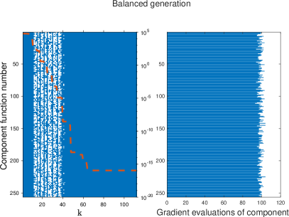
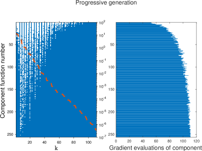
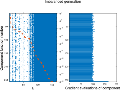
Figure 4.1: Statistics of a single run of algorithm 1 with first-order models FO for each of the three different modes of problem data generation for logistic loss functions. In each of the three pairs of figures, the left figure juxtaposes the optimality gap $f(x^{k})-f(x^{*})$ on top of the sparsity pattern of the evaluations $(F_{i}(x^{k}),\nabla F_{i}(x^{k}))$ performed in the $k$th point queried by the algorithm. The histogram in the right figure of each pair illustrates a sum of the corresponding sparsity pattern, namely, the total number of ($F_{i}(x),\nabla F_{i}(x)$) evaluations performed.

In Figure 4.1 we illustrate the first-order method on a logistic loss function defined by a single realization of problem data $\{(\bm{a}_{x,i},\bm{a}_{y,i})\}_{i=1}^{p}$ under each of the three modes of generation. We note in Figure 4.1 that, as should be expected by our error bounds FO (see 7, 8), the distribution of the sampled function/gradient evaluations $(F_{i}(\bm{x}^{k}),\nabla F_{i}(\bm{x}^{k}))$ appears to be proportional to the distribution of the Lipschitz constants $L_{i}$. Moreover, we notice that in the balanced setting, the method tends to sample fairly densely on most iterations, whereas in the progressive and imbalanced settings, the method is remarkably sparser in sampling.

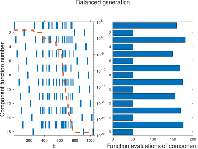
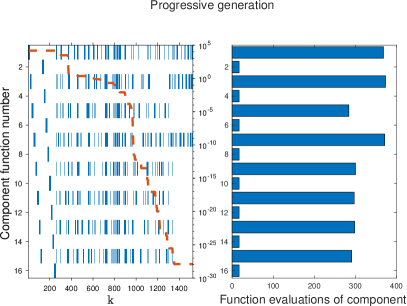
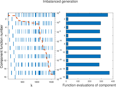
Figure 4.2: Statistics of a single run of algorithm 1 using POUNDERS routines for model building for each of the three different modes of problem data generation for the generalized Rosenbrock function. The interpretation of the plots is the same as in Figure 4.1 except that we now perform only function evaluations (as opposed to gradient evaluations) at a queried point $x^{k}$.

In Figure 4.2, we illustrate the POUNDERS extension on the generalized Rosenbrock function with parameters $\alpha_{i}$ defined by each of the three modes of generation. As expected from the error bounds for ZOGN (that is, 17 and 18), we see that the even-numbered component functions with $L_{i}=0$ are sampled only at the beginning of the algorithm (to construct an initial model) and sometimes at the end of the algorithm (due to criticality checks performed by POUNDERS). However, likely because of the additional multiplicative presence of $|f_{i}(\bm{c}_{i}^{k})|$ in the error bounds, it is not the case—as in Figure 4.1—that the remaining sampling of the odd-numbered component functions is sampled proportionally to their corresponding Lipschitz constants $L_{i}$.

4.4 Comparing SAM-FO with SAG

Because SAM-FO and SAG employ essentially the same average model, it is worth beginning our experiments with a quick comparison of the two methods. Because SAM-FO has globalization via a trust region and can employ knowledge of Lipschitz constants of $L_{i}$, the most appropriate comparison is with the method referred to as SAG-LS (Lipschitz) in [24], which employs a Lipschitz line search for globalization and can employ knowledge of $L_{i}$. We used the implementation of SAG-LS (Lipschitz) associated with [24]. Because SAG-LS (Lipschitz) effectively only updates one model at a time, we choose to compare SAG-LS (Lipschitz) only with SAM-FO with a computational resource size $r=1$ and the dynamic mode of generating $I_{k},J_{k}$ (since the uniform mode disregards $L_{i}$).

Results are shown in Figure 4.3. Throughout these, we use the term effective data passes to refer to the number of component function evaluations performed, divided by $p$, the total number of component functions. With this convention, a deterministic method that evaluates all $p$ component function evaluations in every iteration performs exactly one effective data pass per iteration. Although effective data passes are certainly related to the notion of an epoch in machine learning literature, they differ in that an epoch typically involves some shuffling so that all data points (or, in our setting, component function evaluations) are touched once per effective data pass. This notion of equal touching is not applicable to our randomized methods.

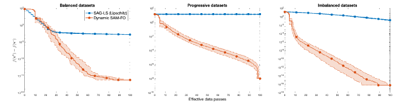
Figure 4.3: Comparing SAG-LS (Lipschitz) with SAM-FO with dynamic batch sizes on logistic loss problems with left) balanced data generation, center) progressive data generation, and right) imbalanced data generation. Solid lines and markers denote median performance across the 90 problems (30 random datasets $\times$ 3 random seeds per dataset), while the outer bands denote $25^{th}--75^{th}$ percentile performance. We note that on the $x$-axis, $f(\bm{x}^{k})-f(\bm{x}^{*})$ is an appropriate metric because these logistic loss test problems are strongly convex.

We note in Figure 4.3 that while SAM-FO clearly outperforms the out-of-the-box version of SAG-LS (Lipschitz) in these experiments when measured in component function evaluations, this does not suggest that SAM-FO would be a preferable method to SAG-LS (Lipschitz) in supervised machine learning (finite-sum minimization) problems. Clearly, SAM-FO involves nontrivial computational and storage overhead in maintaining separate models and computing error bounds; and when the number of examples in a dataset is huge (as is often the case in machine learning settings), this overhead might become prohibitive. Thus, although we can demonstrate that for problems with hundreds (or perhaps thousands) of examples, SAM-FO is the preferable method, we do not want the reader to extrapolate to huge-scale machine learning problems.

4.5 Comparing uniform SAM with dynamic SAM

We now compare both variants of SAM with themselves when generating batches of a fixed computational resource size uniformly at random versus when generating batches according to our suggested algorithm 3.

4.5.1 SAM-FO on logistic loss problems

We first illustrate the performance of SAM-FO under these two randomized batch selection schemes on the logistic loss problems, in other words, the same computational setup as in Section 4.4. Results are shown in Figure 4.4.

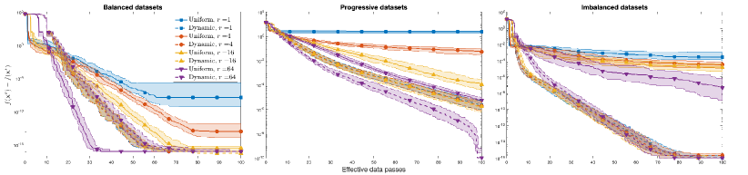
Figure 4.4: Comparing the performance of SAM-FO with itself when using uniform generation of batches of a fixed resource-size $r$ versus generating batches according to algorithm 3 with parameter $r$. We show results using the same percentile bands as in Figure 4.3 and separate results by the mode of generating the dataset (balanced, progressive, or imbalanced Lipschitz constants).

For the runs using balanced data in Figure 4.4, we observe that—perhaps unsurprisingly—for larger values of computational resource size $r$, uniform sampling is marginally better than dynamic sampling. This phenomenon might be explained by the fact that, with all Lipschitz constants roughly the same, the probabilities assigned by algorithm 3 are more influenced by the distance between $x^{k}$ and $y_{i}^{k}$ than anything else, and so “on average” the updates are nearly cyclic. For the progressive datasets in the same figure, we see a more obvious preference for the dynamic variant of SAM-FO across values of $r$. For the imbalanced datasets in the same figure, we still see the same preference, but we notice that the dynamic variant of SAM-FO hardly loses any performance between $r=1$ and $r=128$; this was expected because as long as a batch includes the component function with the large Lipschitz constant “on most iterations,” then the method should be relatively unaffected by the computational resource size $r$.

In Figure 4.5, we display less traditional plots, which we now explain. We introduce the notion of machine size, which we define as the number of component function evaluations that can be made embarrassingly parallel on a theoretical hardware architecture. We make the simplifying assumption that each component function evaluation requires an equal amount of computational resources to perform, which is approximately correct for the test problems in this paper. With the notion of machine size, we can then define the number of rounds required by a dynamic SAM variant with resource size parameter $r$ to solve a problem $\pi$ to a defined level of tolerance $\tau$, when run on a machine of a given machine size $\mu$; that is,

$$R_{r,\pi,\tau,\mu}=\left(\#\text{batches of size $r$ required to satisfy $f(\bm{x}^{k})-f(\bm{x}^{*})\leq\tau$ on problem }\pi\right)\left\lceil\displaystyle\frac{r}{\mu}\right\rceil.$$

The number of rounds $R_{r,\pi,\tau,\mu}$ is an idealized estimation of wall-clock time for estimating scalability. For example, for the logistic loss problem with $p=256$, then 256 function evaluations could be done in the same amount of time required by a single-component function evaluation given a machine size of $\mu=256$. On the other extreme, if $\mu=1$, then 256 function evaluations would require the amount of time required by 256 single-component function evaluations (that is, they would have to be executed serially).

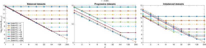
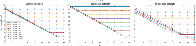
Figure 4.5: For each mode of generating random tested logistic loss problems, we show the median, over the problems $\pi$, of $\log_{2}(R_{r,\pi,\tau,\mu})$. The top row displays results for a convergence tolerance $\tau=10^{-3}$, and the bottom row displays results for the tighter convergence tolerance $\tau=10^{-7}$.

We remark in Figure 4.5 that when using balanced datasets, for all tested values of $r$, SAM-FO-$r$ requires roughly $90\%$ of the computational resource use of the deterministic method in its median performance whenever $r\geq\mu$ for the tighter tolerance $\tau=10^{-7}$. More starkly, when using imbalanced datasets, SAM-FO uses between $40\%$ and $80\%$ of the computational resources required by the deterministic method when $\mu\leq r\leq 128$. Perhaps as expected, results are less satisfactory for the progressive datasets, which are arguably the hardest of these problems. Even for the progressive datasets, however, the regret is not unbearably high in the tighter convergence tolerance, with SAM-FO-$r$ requiring $130\%$ of the computational resources required by the deterministic method when $\mu\leq r\leq 32$, and the randomized and deterministic method roughly breaking even for $\mu\leq r\in\{64,128\}$.

4.5.2 SAM-POUNDERS on Rosenbrock problems

We now illustrate the performance of SAM-POUNDERS under the two randomized batch selection schemes on the Rosenbrock problems. Results are shown in Figure 4.6.

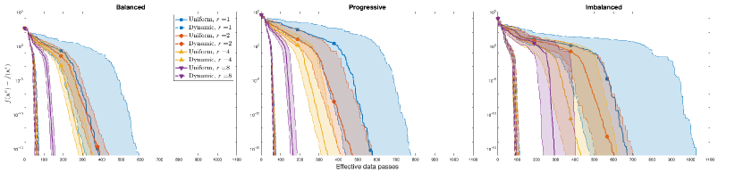
Figure 4.6: Comparing the performance of SAM-POUNDERS with itself when using uniform generation of batches of a fixed resource size $r$ versus generating batches according to algorithm 3 with the Rosenbrock problems. We verified that no run converged to a local minimum, and hence the optimality gap on the $y$-axis is appropriate.

We remark in Figure 4.6 that there is a generally clear preference for employing the dynamic batch selection method over simple uniform batch selection.

We again employ the same comparisons of SAM-POUNDERS-$r$ to POUNDERS as in Figure 4.5 in Figure 4.7.

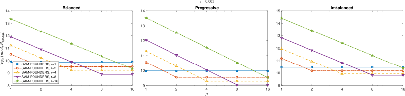
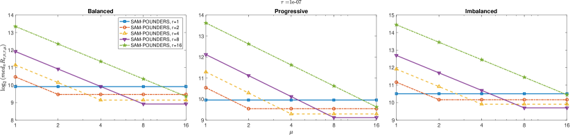
Figure 4.7: For each mode of generating generalized Rosenbrock problems, we show the median, over the problems $\pi$, of $\log_{2}(R_{r,\pi,\tau,\mu})$. The top row displays results for a convergence tolerance $\tau=10^{-3}$, and the bottom row displays results for the tighter convergence tolerance $\tau=10^{-7}$.

We remark that the results shown in Figure 4.7 are satisfactory, with all problems and values of $r$ giving a strict improvement in computational resource use to attain either $\tau=10^{-1}$-optimality or $\tau=10^{-7}$-optimality over the deterministic method.

4.5.3 SAM-POUNDERS on cube problems

We illustrate the performance of
SAM-POUNDERS under the two randomized batch selection schemes on the cube problems. Results are shown in Figure 4.8.

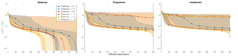
Figure 4.8: Comparing the performance of SAM-POUNDERS with itself when using uniform generation of batches of a fixed resource-size $r$ versus generating batches according to algorithm 3 with the cube problems. We verified that no run converged to a local minimum, and hence the optimality gap on the $y$-axis is appropriate.

As in the Rosenbrock tests, we find in Figure 4.8 a preference for employing the dynamic batch selection method over simple uniform batch selection on the cube problems.

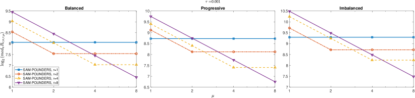
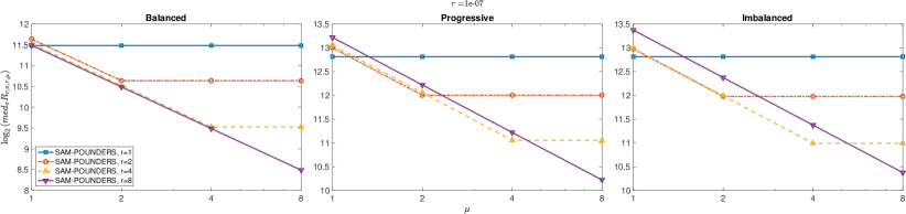
Figure 4.9: For each mode of generating cube problems, we show the median, over the problems $\pi$, of $\log_{2}(R_{r,\pi,\tau,\mu})$. The top row displays results for a convergence tolerance $\tau=10^{-3}$, and the bottom row displays results for the tighter convergence tolerance $\tau=10^{-7}$.

In Figure 4.9, we see that compared with the deterministic method, for the weaker convergence tolerance ($\tau=10^{-3}$) the dynamic variants of SAM-POUNDERS-$r$ yield better median performance than deterministic POUNDERS. However, the situation is more mixed in the tighter convergence tolerance ($\tau=10^{-7}$). While SAM-POUNDERS-$r$ exhibits better median performance than does deterministic POUNDERS for all $r$ in the imbalanced generation setting, the same is only true for $r=1$ in the balanced case and $r=1,2$ in the progressive generation setting. As in the logistic loss experiments, however, we see that even in the situations where SAM-POUNDERS-$r$ does not outperform the deterministic method, it does not lose by a significant amount, leading to low regret.

4.6 Performance of SAM when not assuming knowledge of $L_{i}$

Until now, we have given the SAM methods access to global Lipschitz constants $L_{i}$ in order to compute the various bounds employed in the dynamic batch selection variants. However, assuming access to $L_{i}$ is typically an impractical assumption: while it is practical in the logistic loss problems, it is virtually never practical in any setting of derivative-free optimization.

Thus, we experiment with a simple modification to any given SAM method. Rather than assuming a value of $L_{i}$ at the beginning of the algorithm, we employ estimates $\tilde{L}_{i}$. We arbitrarily initialize $\tilde{L}_{i}=1$ for $i=1,\dots,p$. We select $I_{0}=\{1,\dots,p\}$ on the first iteration and additionally select $I_{k_{0}+1}=\{1,\dots,p\}$, where $k_{0}$ denotes the first successful iteration of algorithm 1. In other words, we are guaranteed at the start of the algorithm to have computed a model of each component function centered at two distinct points; that is, we will have computed $m_{i}(\bm{x};\bm{x}^{0})$ and $m_{i}(\bm{x};\bm{x}^{k_{0}-1})$ for $i=1,\dots,p$. Immediately after updating the models indexed by $I_{k_{0}+1}$, we compute a lower bound on a global Lipschitz constant via the secant

$$\tilde{L}_{i}\leftarrow\displaystyle\frac{\|\nabla m_{i}(\bm{x};\bm{x}^{k_{0}+1})-\nabla m_{i}(\bm{x};\bm{x}^{0})\|}{\|\bm{x}^{k_{0}+1}-\bm{x}^{0}\|}.$$

Over the remainder of the algorithm, on each iteration $k$ in which $i\in I_{k}$, and immediately after updating the $i$th model, we update

$$\tilde{L}_{i}\leftarrow\max\left\{\tilde{L}_{i},\displaystyle\frac{\|\nabla m_{i}(\bm{x};\bm{x}^{k})-\nabla m_{i}(\bm{x};\bm{c}^{k}_{i})\|}{\|\bm{x}^{k}-\bm{c}^{k}_{i}\|}\right\},$$

provided that $\bm{x}^{k}\neq\bm{c}^{k}_{i}$.

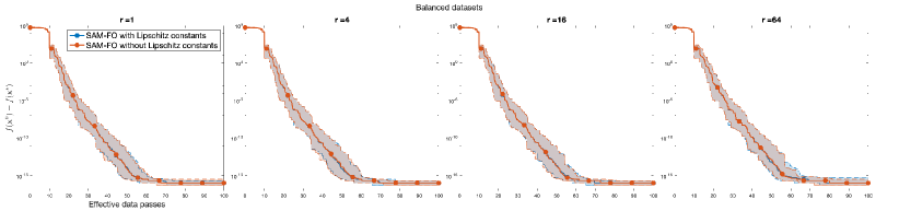
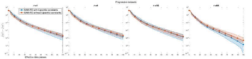
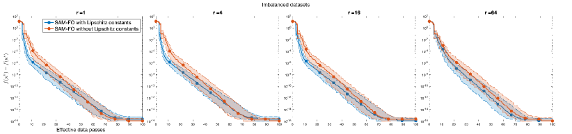
Figure 4.10: Comparing the performance of SAM-FO with dynamic batch selection and resource size $r$ with itself when provided with Lipschitz constants and when using our proposed scheme to dynamically adjust the Lipschitz constant estimates. We show results using the same percentile bands as in Figure 4.3 and again separate results by the mode of generating the dataset (balanced, progressive, or imbalanced Lipschitz constants).

In Figure 4.10 we first illustrate results for the logistic loss problems. Remarkably, there is little difference in performance in the balanced dataset case. When we move to progressive datasets, it is remarkable that in median performance, and with the possible exception of $r=64$, the performance of SAM-FO-$r$ is typically better without assuming Lipschitz constants than with assuming them explicitly. This is not completely bizarre, however, as the global Lipschitz constants $L_{i}$ provided to any method are necessarily worst-case upper bounds on local Lipschitz constants, and it is generally unlikely that a method will encounter the upper bound—hence, the component functions with larger $L_{i}$ values (i.e., those with indices closer to $p$) may be updated more frequently than they need to be in the randomized methods, leading to slowdowns when $L_{i}$ is available. In the imbalanced datasets test, we see that SAM-FO-$r$ indeed loses some performance when using estimates $\tilde{L}_{i}$, but not drastically. A reasonable explanation for this phenomenon is that the overapproximation provided by $L_{i}$ that proved to be potentially problematic in the progressive dataset is in fact helpful in the imbalanced datasets—indeed we want to be updating the $p$th model with much higher frequency relative to the other $p-1$ components over the run of the algorithm, and so a relatively large value of $L_{i}$ provided by a global Lipschitz constant will certainly force this to happen.

For the sake of space in the main body of text, we move the results of these experiments for the remaining two classes of problems with SAM-POUNDERS (generalized Rosenbrock and cube) to the Appendix. It suffices to say that in all cases, there is some loss in performance by replacing $L_{i}$ with the coarse estimate $\tilde{L}_{i}$, but the loss in most cases is acceptable.

Appendix A Proof of theorem 3.1

Proof.

We will first derive a bound on $\|\nabla F_{i}(\bm{x})-\bm{g}_{i}^{k}(\bm{c}^{k}_{i};\delta_{i})\|$. By 3.0.1, $\hat{V}_{Y_{i}}(\bm{x};\bm{c}^{k}_{i})$ is invertible, regardless of $\bm{x}$ and $\delta_{i}>0$. Setting up the linear interpolation system, we see that

$$(\bm{v}^{j}-\bm{c}_{i}^{k})^{\top}\bm{g}_{i}^{k}(\bm{c}^{k}_{i};\delta_{i})=F_{i}(\bm{v}^{j})-F_{i}(\bm{c}^{k}_{i}),\quad j=1,\dots,n.$$

By the mean value theorem, this right-hand side is also equal to

$$F_{i}(\bm{v}^{j})-F_{i}(\bm{c}^{k}_{i})=\displaystyle\int_{0}^{1}(\bm{v}^{j}-\bm{c}^{k}_{i})^{\top}\nabla F_{i}(\bm{c}^{k}_{i}+t(\bm{v}^{j}-\bm{c}^{k}_{i}))\mathrm{d}t,\quad j=1,\dots,n,$$

and so, by 2.0.1,

$$(\bm{v}^{j}-\bm{c}^{k}_{k})^{\top}(\nabla F_{i}(\bm{c}^{k}_{i})-\bm{g}_{i}^{k}(\bm{c}^{k}_{i};\delta_{i}))\leq\frac{L_{i}}{2}\|\bm{v}^{j}-\bm{c}^{k}_{i}\|^{2},\quad j=1,\dots,n.$$

Combining these $n$ inequalities, noting that $\|\bm{v}^{j}-\bm{c}^{k}_{i}\|^{2}\leq\delta_{i}$ for $j=1,\dots,n$, and recalling the definition of $\hat{V}_{Y_{i}}(\bm{x};\bm{c}^{k}_{i})$ in 14,

$$\|\hat{V}_{Y_{i}}(\bm{x};\bm{c}^{k}_{i})(\nabla F_{i}(\bm{c}^{k}_{i})-\bm{g}_{i}^{k}(\bm{c}^{k}_{i};\delta_{i}))\|\leq\frac{L_{i}\sqrt{n}}{2\max\{\delta_{i},\|\bm{x}-\bm{c}^{k}_{i}\|\}}\delta_{i}^{2},$$

and so

$$\|\nabla F_{i}(\bm{c}^{k}_{i})-\bm{g}_{i}^{k}(\bm{c}^{k}_{i};\delta_{i})\|\leq\frac{L_{i}\sqrt{n}\|\hat{V}_{Y_{i}}^{-1}(\bm{x};\bm{c}^{k}_{i})\|}{2\max\{\delta_{i},\|\bm{x}-\bm{c}^{k}_{i}\|\}}\delta_{i}^{2}.$$ (23)

Thus, for any $\bm{x}\in\mathbb{R}^{n}$,

$$\begin{array}[]{lll}\|\nabla F_{i}(\bm{x})-\bm{g}_{i}^{k}(\bm{c}^{k}_{i};\delta_{i})\|&\leq&\|\nabla F_{i}(\bm{x})-\nabla F_{i}(\bm{c}^{k}_{i})\|+\|\nabla F_{i}(\bm{c}^{k}_{i})-\bm{g}_{i}^{k}(\bm{c}^{k}_{i};\delta_{i})\|\\ &\leq&L_{i}\left(\|\bm{x}-\bm{c}^{k}_{i}\|+\frac{\sqrt{n}\|\hat{V}_{Y_{i}}^{-1}(\bm{x};\bm{c}^{k}_{i})\|}{2\max\{\delta_{i},\|\bm{x}-\bm{c}^{k}_{i}\|\}}\delta_{i}^{2}\right).\end{array}$$ (24)

Now, by Taylor’s theorem,

$$F_{i}(\bm{x})-F_{i}(\bm{c}^{k}_{i})\leq\nabla F_{i}(\bm{c}^{k}_{i})^{\top}(\bm{x}-\bm{c}^{k}_{i})+\frac{L_{i}}{2}\|\bm{x}-\bm{c}^{k}_{i}\|^{2}.$$

Combined with 24,

$$\begin{array}[]{lll}F_{i}(\bm{x})-m_{i}(\bm{x};\bm{c}^{k}_{i})&=&F_{i}(\bm{x})-F_{i}(\bm{c}^{k}_{i})-\bm{g}_{i}^{k}(\bm{c}^{k}_{i};\delta_{i})^{\top}(\bm{x}-\bm{c}^{k}_{i})\\ &\leq&(\nabla F_{i}(\bm{c}^{k}_{i})-\bm{g}(\bm{c}^{k}_{i};\delta_{i}))^{\top}(\bm{x}-\bm{c}^{k}_{i})+\frac{L_{i}}{2}\|\bm{x}-\bm{c}^{k}_{i}\|^{2}.\\ &\leq&L_{i}\left(\|\bm{x}-\bm{c}^{k}_{i}\|+\frac{\sqrt{n}\|\hat{V}_{Y_{i}}^{-1}(\bm{x};\bm{c}^{k}_{i})\|}{2\max\{\delta_{i},\|\bm{x}-\bm{c}^{k}_{i}\|\}}\delta_{i}^{2}\right)\|\bm{x}-\bm{c}^{k}_{i}\|+\frac{L_{i}}{2}\|\bm{x}-\bm{c}^{k}_{i}\|^{2}.\end{array}$$

The theorem follows. ∎

Appendix B Statement of algorithm 4

The algorithm of [9, 14] essentially amounts to finding the solution $\tilde{\bm{\pi}}\in\mathbb{R}^{p}$ to the equation

$$\Psi_{b}(\tilde{\bm{\pi}})=\bm{\pi},$$ (25)

where in our notation, $b$ is the desired batch size, and $\bm{\pi}$ are the desired inclusion probabilities. $\Psi_{b}$ is defined recursively and entrywise via

$$\Psi_{0}(\tilde{\bm{\pi}})=\mathbf{0}_{p},\quad[\Psi_{k}(\tilde{\bm{\pi}})]_{i}=k\displaystyle\frac{\displaystyle\frac{\tilde{\pi}_{i}}{1-\tilde{\pi}_{i}}\left(1-[\Psi_{k-1}(\tilde{\bm{\pi}})]_{i}\right)}{\displaystyle\sum_{j=1}^{p}\frac{\tilde{\pi}_{j}}{1-\tilde{\pi}_{j}}\left(1-[\Psi_{k-1}(\tilde{\bm{\pi}})]_{j}\right)},\quad k=1,2,\dots,b.$$ (26)

The pseudocode for algorithm 4 is provided in this section.

Input: Batch size $b>0$, probability vector $\bm{\pi}\in\mathbb{R}^{p}$.

Initialize $\tilde{\bm{\pi}}\leftarrow\mathbf{0}_{p}$.

$A\leftarrow\{i:\pi_{i}=1\},B\leftarrow\{1,2,\dots,p\}\setminus A,\tilde{\bm{\pi}}_{A}\leftarrow\bm{\pi}_{A}$.

if $|A|=b$ then

      return $\tilde{\bm{\pi}}$

end if

Compute $\tilde{\pi}_{B}^{*}$ such that $\Psi_{b-|A|}(\tilde{\bm{\pi}}_{B}^{*})=\bm{\pi}_{B}.$

$\bm{\lambda}\leftarrow\log\left(\displaystyle\frac{\tilde{\bm{\pi}}_{B}^{*}}{\mathbf{1}_{|B|}-\tilde{\bm{\pi}}_{B}^{*}}\right)$ ($\log$ and division interpreted entrywise)

Compute scalar $c$ such that

$$b-|A|=\displaystyle\sum_{i\in B}\frac{\exp\left(\lambda_{i}+c\right)}{1+\exp\left(\lambda_{i}+c\right)}.$$ (27)

$\tilde{\bm{\pi}}_{B}^{*}\leftarrow\displaystyle\frac{\exp(\bm{\lambda}+c\mathbf{1}_{|B|})}{\mathbf{1}_{|B|}+\exp(\bm{\lambda}+c\mathbf{1}_{|B|})}$ ($\exp$ and division interpreted entrywise)

$\tilde{\bm{\pi}}_{B}\leftarrow\tilde{\bm{\pi}}_{B}^{*}$.

return $\tilde{\bm{\pi}}$

Algorithm 4 Transforming $\bm{\pi}$ into $\tilde{\bm{\pi}}$

algorithm 4 simply solves 25 after preprocessing any $\tilde{\pi}_{i}=1$, a clearly necessary step in light of 26. In our experiments, we used a basic implementation of Newton’s method with a backtracking line search for the solution of 25. As mentioned in the main body of the text, we then do some postprocessing to force

$$\sum_{i=1}^{p}\tilde{\pi}_{i}^{k}=b.$$

Although technical, the reasoning for why this postprocessing is valid is due to the fact that Poisson sampling is a special case of exponential sampling with a nontrivial affine subspace invariant under the exponential pdf; this is is well-explained in, for instance, [25][Section 5.6.3]. In our experiments, we also solve (27) by a basic implementation of Newton’s method with a backtracking line search.

Appendix C Additional Numerical Results

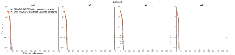
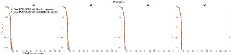
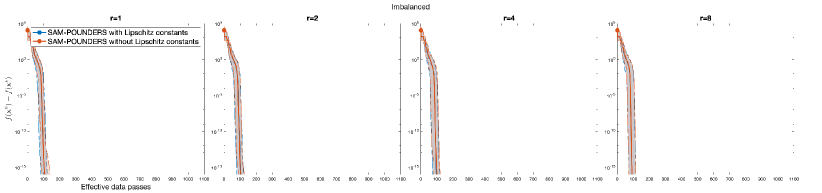
Figure C.1: Comparing the performance of SAM-POUNDERS with dynamic batch selection and resource size $r$ with itself when provided with Lipschitz constants and when using our proposed scheme to dynamically adjust the Lipschitz constant estimates. These results show performance on the generalized Rosenbrock problems.

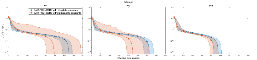
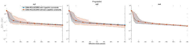
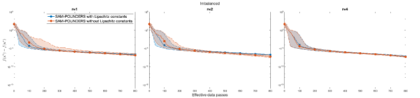
Figure C.2: Comparing the performance of SAM-POUNDERS with dynamic batch selection and resource size $r$ with itself when provided with Lipschitz constants and when using our proposed scheme to dynamically adjust the Lipschitz constant estimates. These results show performance on the cube problems.

In both Figure C.1 and Figure C.2, we intentionally leave the $x$-axis identical to the one employed in Figure 4.6 and Figure 4.8, for easy visual comparison. We see that while in all cases, some performance is lost when access to $L_{i}$ is taken away, the median performance of a dynamic variant without global Lipschitz constants is still always better than the median performance of the same method with uniform sampling.

The submitted manuscript has been created by UChicago Argonne, LLC, Operator of Argonne National Laboratory (“Argonne”). Argonne, a U.S. Department of Energy Office of Science laboratory, is operated under Contract No. DE-AC02-06CH11357. The U.S. Government retains for itself, and others acting on its behalf, a paid-up nonexclusive, irrevocable worldwide license in said article to reproduce, prepare derivative works, distribute copies to the public, and perform publicly and display publicly, by or on behalf of the Government. The Department of Energy will provide public access to these results of federally sponsored research in accordance with the DOE Public Access Plan http://energy.gov/downloads/doe-public-access-plan.

References

- Aires [1999] N. Aires. Algorithms to find exact inclusion probabilities for conditional Poisson sampling and Pareto ps sampling designs. Methodology and Computing in Applied Probability, 1(4):457–469, 1999. doi:10.1023/A:1010091628740.
- [2] J. Blanchet, C. Cartis, M. Menickelly, and K. Scheinberg. Convergence rate analysis of a stochastic trust-region method via supermartingales. INFORMS Journal on Optimization, 1(2):92–119. doi:10.1287/ijoo.2019.0016.
- Bollapragada et al. [2020] R. Bollapragada, M. Menickelly, W. Nazarewicz, J. O’Neal, P.-G. Reinhard, and S. M. Wild. Optimization and supervised machine learning methods for fitting numerical physics models without derivatives. Journal of Physics G: Nuclear and Particle Physics, 48(2):024001, Dec 2020. doi:10.1088/1361-6471/abd009. URL https://doi.org/10.1088/1361-6471/abd009.
- Bottou and Bousquet [2007] L. Bottou and O. Bousquet. The tradeoffs of large scale learning. Advances in neural information processing systems, 20, 2007.
- [5] L. Bottou, F. E. Curtis, and J. Nocedal. Optimization methods for large-scale machine learning. SIAM Review, 60(2):223–311. doi:10.1137/16m1080173.
- Bouhlel et al. [2019] M. A. Bouhlel, J. T. Hwang, N. Bartoli, R. Lafage, J. Morlier, and J. R. Martins. A python surrogate modeling framework with derivatives. Advances in Engineering Software, 135:102662, Sept. 2019. doi:10.1016/j.advengsoft.2019.03.005.
- [7] C. Cartis and L. Roberts. A derivative-free Gauss-Newton method. Mathematical Programming Computation, 11(4):631–674. doi:10.1007/s12532-019-00161-7.
- [8] R. Chen, M. Menickelly, and K. Scheinberg. Stochastic optimization using a trust-region method and random models. Mathematical Programming, 169(2):447–487. doi:10.1007/s10107-017-1141-8.
- Chen [2000] S. X. Chen. General properties and estimation of conditional bernoulli models. Journal of Multivariate Analysis, 74(1):69–87, 2000.
- Chen et al. [1994] X.-H. Chen, A. P. Dempster, and J. S. Liu. Weighted finite population sampling to maximize entropy. Biometrika, 81(3):457–469, 1994.
- [11] A. R. Conn, K. Scheinberg, and L. N. Vicente. Introduction to Derivative-Free Optimization. SIAM. doi:10.1137/1.9780898718768.
- Csiba and Richtárik [2018] D. Csiba and P. Richtárik. Importance sampling for minibatches. Journal of Machine Learning Research, 19(27):1–21, 2018. URL http://jmlr.org/papers/v19/16-241.html.
- [13] A. Defazio, F. R. Bach, and S. Lacoste-Julien. SAGA: A fast incremental gradient method with support for non-strongly convex composite objectives. In Z. Ghahramani, M. Welling, C. Cortes, N. D. Lawrence, and K. Q. Weinberger, editors, Advances in Neural Information Processing Systems 27, pages 1646–1654. URL http://papers.nips.cc/paper/5258-saga-a-fast-incremental-gradient-method-with-support-for-non-strongly-convex-composite-objectives.
- Deville [2000] J.-C. Deville. Note sur l’algorithme de chen, dempster et liu. Document de travail non publié, 2000.
- [15] S. Ghadimi and G. Lan. Stochastic first- and zeroth-order methods for nonconvex stochastic programming. SIAM Journal on Optimization, 23(4):2341–2368. doi:10.1137/120880811.
- Hanzely and Richtarik [2019] F. Hanzely and P. Richtarik. Accelerated coordinate descent with arbitrary sampling and best rates for minibatches. In K. Chaudhuri and M. Sugiyama, editors, Proceedings of the Twenty-Second International Conference on Artificial Intelligence and Statistics, volume 89 of Proceedings of Machine Learning Research, pages 304–312. PMLR, 16–18 Apr 2019. URL https://proceedings.mlr.press/v89/hanzely19a.html.
- Horváth and Richtarik [2019] S. Horváth and P. Richtarik. Nonconvex variance reduced optimization with arbitrary sampling. In K. Chaudhuri and R. Salakhutdinov, editors, Proceedings of the 36th International Conference on Machine Learning, volume 97 of Proceedings of Machine Learning Research, pages 2781–2789. PMLR, 09–15 Jun 2019. URL https://proceedings.mlr.press/v97/horvath19a.html.
- [18] R. Johnson and T. Zhang. Accelerating stochastic gradient descent using predictive variance reduction. In C. J. C. Burges, L. Bottou, M. Welling, Z. Ghahramani, and K. Q. Weinberger, editors, Advances in Neural Information Processing Systems 26, volume 26, pages 315–323. Curran Associates, Inc.
- [19] J. Kiefer and J. Wolfowitz. Stochastic estimation of the maximum of a regression function. The Annals of Mathematical Statistics, 22(3):462–466. doi:10.1214/aoms/1177729392.
- Needell et al. [2014] D. Needell, R. Ward, and N. Srebro. Stochastic gradient descent, weighted sampling, and the randomized kaczmarz algorithm. In Z. Ghahramani, M. Welling, C. Cortes, N. Lawrence, and K. Weinberger, editors, Advances in Neural Information Processing Systems, volume 27. Curran Associates, Inc., 2014. URL https://proceedings.neurips.cc/paper/2014/file/f29c21d4897f78948b91f03172341b7b-Paper.pdf.
- Richtárik and Takáč [2016] P. Richtárik and M. Takáč. On optimal probabilities in stochastic coordinate descent methods. Optimization Letters, 10(6):1233–1243, 2016.
- [22] H. Robbins and S. Monro. A stochastic approximation method. The Annals of Mathematical Statistics, 22(3):400–407. doi:10.1214/aoms/1177729586.
- Roux et al. [2012] N. Roux, M. Schmidt, and F. Bach. A stochastic gradient method with an exponential convergence _rate for finite training sets. Advances in Neural Information Processing Systems, 25, 2012.
- Schmidt et al. [2017] M. Schmidt, N. L. Roux, and F. Bach. Minimizing finite sums with the stochastic average gradient. Mathematical Programming, 162(1-2):83–112, 2017. doi:10.1007/s10107-016-1030-6.
- Tillé [2006] Y. Tillé. Sampling algorithms. Springer, 2006.
- [26] S. M. Wild. Solving derivative-free nonlinear least squares problems with POUNDERS. In T. Terlaky, M. F. Anjos, and S. Ahmed, editors, Advances and Trends in Optimization with Engineering Applications, pages 529–540. SIAM. doi:10.1137/1.9781611974683.ch40.
- [27] H. Zhang and A. R. Conn. On the local convergence of a derivative-free algorithm for least-squares minimization. Computational Optimization and Applications, 51(2):481–507. doi:10.1007/s10589-010-9367-x.
- [28] H. Zhang, A. R. Conn, and K. Scheinberg. A derivative-free algorithm for least-squares minimization. SIAM Journal on Optimization, 20(6):3555–3576. doi:10.1137/09075531X.
- Zhang et al. [2013] L. Zhang, M. Mahdavi, and R. Jin. Linear convergence with condition number independent access of full gradients. Advances in Neural Information Processing Systems, 26, 2013.