Uncertainty quantification for mineral precipitation and dissolution in fractured porous media

Abstract

In this work, we present an uncertainty quantification analysis to determine the influence and importance of some physical parameters in a reactive transport model in fractured porous media. An accurate description of flow and transport in the fractures is key to obtain reliable simulations, however, fractures geometry and physical characteristics pose several challenges from both the modeling and implementation side. We adopt a mixed-dimensional approximation, where fractures and their intersections are represented as objects of lower dimension. To simplify the presentation, we consider only two chemical species: one solute, transported by water, and one precipitate attached to the solid skeleton. A global sensitivity analysis to uncertain input data is performed exploiting the Polynomial Chaos expansion along with spectral projection methods on sparse grids.

1 Introduction

The Paris agreement, adopted by 196 parties in 2015, aims at limiting global warming to below 2${}^{\circ}C$, preferably to 1.5${}^{\circ}C$, compared to pre-industrial levels. The reduction of greenhouse gas emissions in the atmosphere is crucial to achieve such long term goal, and requires the transition towards renewable energies, and the subsequent need for effective energy storage; moreover, a safe long term sequestration of $CO_{2}$ is considered a promising strategy to reduce emissions into the atmosphere. Many of the aforementioned strategies entail a massive use of the subsurface for fluids injection, storage and production. If, on one hand, it is necessary to guarantee the mechanical integrity of the subsurface to avoid unwanted fracturing and induced seismicity, it is also important to evaluate the effect of chemical reactions on the hydraulic properties of the porous media. Indeed, the injection of water at different temperature and with different solutes concentration with respect to the formation can cause dissolution and precipitation of minerals, with an impact on porosity and permeability. In some cases, as in the case of in situ carbon mineralization, these reactions can be exploited to our advantage to obtain a better storage of $CO_{2}$ by 1) chemically trapping carbon by binding it into existing mineral and, at the same time 2) thanks to the change of specific volume associated with the transformation of the minerals, creating a more effective cap-rock, [23]. Even if this process occurs over very long time scales in natural conditions, its controlled exploitation is an interesting technological challenge.

A realistic mathematical model of these phenomena encompasses a model for flow in porous media (we focus on single phase flow, assuming small concentrations of gases, if present), coupled with the transport of mobile species and the modeling of both kinetic and equilibrium reactions. Moreover, since reaction rates are usually influenced by temperature, and in view of the possible application of the model to low temperature geothermal plants, the coupled model is completed by the heat equation, [14].

Since fractures are ubiquitous in porous media and have a major impact on flow and transport (both of solutes and heat) this work is focused on the modeling of fractured porous media, where fractures are modeled as lower dimensional objects, which can be much more permeable than the surrounding medium, or nearly impermeable if, for instance, precipitation occurs reducing their aperture, [15].

Many physical, geometrical and geochemical parameters involved in the model are affected by uncertainty, therefore a purely deterministic evaluation of the model is useless without a suitable analysis of the solution variance. In this work we propose an uncertainty quantification workflow based on Polynomial Chaos [30, 18] and sparse grids [6] for the sampling of the parameters space: this choice allows us to obtain accuracy with a manageable number of evaluations of the model, which, being coupled and time dependent, has a non-negligible computational cost. The goal is to compute the Sobol indices associated with some input parameters to quantify the impact of the uncertainty of such quantities on a variable of interest, typically the medium porosity. The space distribution of the Sobol indices, or the partial variances, can also give interesting insight into the problem, which, in spite of being reduced to the minimum possible complexity, already exhibits a non-trivial, fully coupled behavior.

The paper is structured as follows. In Section 2 we present the model equation in a homogeneous porous medium; then, in Section 3, we extend the equations to the hybrid dimensional case to account for the coupling with fractures. Section 4 briefly discusses the proposed numerical approximation schemes and some implementation details. Section 5 describes the uncertainty quantification workflow and Section 6 is devoted to the presentation of a a complete set of test cases. Finally, conclusions are drawn in Section 7.

2 Problem description and mathematical model

We consider the coupled problem of single-phase flow and reactive transport in porous media, accounting for the porosity changes linked to mineral reactions. Single phase flow can be assumed, even in the presence of $CO_{2}$, at low gas concentrations, for instance at the edge of the plume, away from injection wells. Typically, a large number of species is needed for a realistic modeling of reactive transport, including solid mineral species and aqueous complexes, and the chemical reactions include equilibrium and kinetic ones. In the following we will discuss the general case and then specialize the model to the simple case of the dissolution/precipitation of a single mineral species.

2.1 Single phase flow

Under the assumption of single-phase flow, the fluid pressure $p$ and Darcy velocity $\bm{q}$ can be computed as the solution of a Darcy problem

$$\begin{aligned} &\bm{q}+\dfrac{k(\phi)}{\mu}(\nabla p-\rho_{w}g\bm{e}_{z})=0\\ &\nabla\cdot\bm{q}=-\partial_{t}\phi\end{aligned}$$ (1)

complemented by suitable boundary conditions prescribing a given pressure or normal flux on the boundary. Here $k$ is the permeability, $\mu$ the viscosity, $\rho_{w}$ is the fluid density and $g$ is the gravity acceleration. Note that in (1) we have assumed constant density, but we are accounting for porosity changes through a source term. Indeed, porosity depends on the changes of the mineral volume fraction as detailed in Section 2.3.

The intrinsic permeability, which we assume to be isotropic in the bulk porous medium, can be modeled as a function of porosity. We consider the following law

$$k(\phi)=k_{0}\left(\dfrac{\phi}{\phi_{0}}\right)^{2}$$

where $k_{0}$ is the reference value at the initial porosity $\phi_{0}$. Note that this dependence will introduce a non-linear coupling among the model equations.

2.2 Advection-diffusion-reaction equations for mobile species

Let $u_{i}$ denote the molar concentration of the $i$-th mobile species, for instance a dissolved mineral or gas. The governing equation reads

$$\partial_{t}(\phi u_{i})+\nabla\cdot(\bm{q}u_{i}-\phi d\nabla u_{i})=\phi\displaystyle\sum_{r=1}^{N_{r}}\nu_{ir}R_{r}$$ (2)

where $d$ is the diffusion tensor (which may account for mechanical dispersion, and is considered to be the same for all species), $\bm{q}$ is the Darcy velocity, $N_{r}$ is the number of reactions and $\nu_{ir}$ is the stoichiometric coefficient of species $i$ in reaction $r$.

In particular, we consider a set of $N_{r}$ reactions in the form

$$\sum_{i}\nu_{ir}X_{i}\rightleftarrows 0\qquad r=1,\ldots,N_{r}$$

where $X_{i}$ is a generic species, solid or mobile, $\nu_{ir}$ is zero if $X_{i}$ is not involved in the reaction $r$, negative if $X_{i}$ is a reactant in the forward reaction, and positive if it is a product. The reaction rate $R_{r}$ should be interpreted as the net rate, i.e.

$$R_{r}=R_{r}^{+}-R_{r}^{-}$$

where $R_{r}^{+}$ is the forward reaction rate and $R_{r}^{-}$ is the backward one. Their expressions are often empirical and problem dependent; the one considered in this work is illustrated in Section 2.5. Finally, equation (2) should be complemented by initial conditions $u_{i}(\bm{x},0)=u_{i,0}(\bm{x})$, and boundary conditions on the concentration or normal flux.

2.3 Mineral species

In the case the species is immobile the evolution equation for its concentration, denoted as $w_{i}$, reduces to an ordinary differential equation since we do not have the transport and diffusion terms, i.e.

$$d_{t}(\phi w_{i})=\phi\displaystyle\sum_{r=1}^{N_{r}}\nu_{ir}R_{r}$$ (3)

where an initial condition is supplemented as $w_{i}(\bm{x},0)=w_{i,0}(\bm{x})$. However, it may be more convenient to consider a different measure of concentration for solid species, in particular we want to compute the solid volume fractions $\phi_{i}$ as the ratio of the volume of mineral $i$ for a unit volume of rock. The volume fractions can be obtained from the concentrations as

$$\phi_{i}=w_{i}\eta_{i}\phi$$ (4)

where $\eta_{i}$ is the molar volume of the mineral. If we let $\phi_{I}$ be the volume fraction of inert minerals (i.e. species that are not affected by chemical reactions) we have that

$$\begin{aligned} &\phi=1-\phi_{I}-\displaystyle\sum_{i=1}^{N_{s}}\phi_{i}\\ &d_{t}\phi=-\displaystyle\sum_{i=1}^{N_{s}}\eta_{i}d_{t}(\phi w_{i})\end{aligned}$$

where $N_{s}$ is the number of solid, immobile species.

2.4 Heat equation

Since reaction rates usually depend on temperature, we include in our model the heat equation for thermal conduction (based on Fourier’s law) and convection in the porous media. We assume thermal equilibrium between rock and water, so that only one equation can be considered instead of two.

The temperature field is indicated as $\theta$ and its evolution is described by

$$\begin{aligned} &\partial_{t}(c(\phi)\theta)+\nabla\cdot(\rho_{w}c_{w}\bm{q}\theta-\Lambda(\phi)\nabla\theta)+j=0.\end{aligned}$$ (5)

Here $c$ is the effective thermal capacity defined as the porosity-weighted average of the water $c_{w}$ and solid $c_{s}$ specific thermal capacities,

$$c(\phi)=\phi\rho_{w}c_{w}+(1-\phi)\rho_{s}c_{s},$$

where $\rho_{w}$ and $\rho_{s}$ are the densities of the water and solid phase respectively. The effective thermal conductivity $\Lambda$ is computed in a similar way, as

$$\Lambda(\phi)=\Lambda_{w}^{\phi}\Lambda_{s}^{1-\phi},$$

where $\Lambda_{s}$ and $\Lambda_{s}$ are the water and solid thermal conductivity. Finally, $j$ models a source or sink of heat in the system. Equation (5) is completed by initial conditions, $\theta(\bm{x},0)=\theta_{0}(\bm{x})$, and boundary conditions on the temperature or heat flux.

2.5 Simplified dissolution-precipitation model

In this work we consider a single, simple kinetic reaction in the form

$$U+V-W\leftrightarrow 0$$

where $U$ and $V$ are the positive and negative ion respectively, and $W$ is the precipitate they can form, [27]. The net reaction rate results from the difference between precipitation (forward reaction) and dissolution (backward reaction). Under the hypotheses of electrical equilibrium, we can assume that the concentration of $U$ and $V$ are equal and denoted by $u$, which from now on is the molar concentration of the mobile species, whereas $w$ is the molar concentration of the precipitate. The reaction rates are modeled as

$$\begin{aligned} &r_{p}=\lambda_{-}(\theta)u^{2}\\ &r_{d}=\lambda_{+}(\theta)\end{aligned}$$

moreover, at equilibrium we have that $r_{d}=r_{p}$, thus, $\lambda^{+}=\lambda$ and $\lambda_{-}=\lambda u_{e}^{-2}$ where $u_{e}$ is the equilibrium solute concentration. The net reaction rate is then

$$r_{w}(u,w,\theta)=\begin{dcases*}\displaystyle\lambda\left(\frac{u^{2}}{u_{e}^{2}}-1\right)&if $w>0$\\ \lambda\frac{u^{2}}{u_{e}^{2}}&if $w\leq 0$.\end{dcases*}$$

Note that precipitation proceeds at a constant rate until $w=0$, and is then set to zero.

2.6 The complete model

The complete model, in the case of our interest, computes $(\bm{q},p,\theta,u,w,\phi)$ by solving the following system of non-linear and coupled equations given by

$$\begin{aligned} &\bm{q}+\dfrac{k(\phi)}{\mu}(\nabla p-\rho g\bm{e}_{z})=0\\ &\nabla\cdot\bm{q}=-\partial_{t}\phi\\ &\partial_{t}[c(\phi)\theta]+\nabla\cdot(\rho_{w}c_{w}\bm{q}\theta-\Lambda(\phi)\nabla\theta)+j=0\\ &\partial_{t}(\phi u)+\nabla\cdot(\bm{q}u-\phi d\nabla u)=-\phi r_{w}(u,w,\theta)\\ &d_{t}(\phi w)=\phi r_{w}(u,w,\theta)\\ &d_{t}\phi=-\eta d_{t}(\phi w)\end{aligned}$$ (6)

complemented by constitutive laws and suitable initial and boundary conditions.

3 Hybrid dimensional model for fractured porous media

In the following we introduce the extension of the coupled model (6) to the case of fractured porous media, following [15]. For the sake of simplicity we will present the model in the case of a single fracture, geometrically reduced to its centerline, see Figure 1. This model reduction strategy is often adopted in the simulation of fractured porous media to reduce the computational cost by avoiding excessive mesh refinement; moreover, in our case it is particularly convenient since the aperture can change in time due to reactions. For more references on this approach see [24, 19, 28, 26, 5, 1, 3, 14] and references therein.

Figure 1: Fractured domain and notation.

Let $\tilde{\Omega}$ be the fractured domain. Following [13], we define $\gamma$ as a non self-intersecting $C^{2}$ curve (if $n=2$) or surface (if $n=3$). In an equi-dimensional setting a fracture can be defined as the following set of points

$$\Gamma=\left\{\bm{x}\in\tilde{\Omega}:\,\bm{x}=\bm{s}+r\bm{n}_{\gamma},\,\bm{s}\in\gamma,\,r\in\left(-\frac{\epsilon_{\gamma}(\bm{s})}{2},\frac{\epsilon_{\gamma}(\bm{s})}{2}\right)\right\}.$$

Thus, we have a subdomain of $\tilde{\Omega}$, separated by the surrounding porous medium $\Omega$ by the interfaces $\gamma_{+}$ and $\gamma_{-}$ with associated normal vectors $\bm{n}_{+}$ and $\bm{n}_{-}$. We replace the fracture $\Gamma$ with its centerline $\gamma$ and we assign a unique normal $\bm{n}_{\gamma}=\bm{n}_{\gamma,+}$ to the fracture, see Figure 1. We assume that the fracture is open, with porosity $\phi_{\gamma}=1$.

3.1 Reduced variables

In the following we denote with the subscript $\gamma$ the variables in the fracture, and with $\Omega$ the variables in the porous medium. Note that, after geometrical reduction, we denote with $\Omega$ the domain $\tilde{\Omega}\setminus\gamma$. Reduced vectors variables in the fracture are defined as the integral of the tangential components of the corresponding equi-dimensional variables,

$$\bm{q}_{\gamma}(\bm{x})\vcentcolon=\int_{\epsilon_{\gamma}(\bm{x})}T(\bm{x})\bm{q}(\bm{x},s)ds$$

with $T\vcentcolon=I-N$ and $N\vcentcolon=\bm{n}_{\gamma}\otimes\bm{n}_{\gamma}$ the tangential and normal projection matrices, respectively. The reduced scalar variables are instead the integral average, for each section of the fracture, of the equi-dimensional counterparts

$$p_{\gamma}(\bm{x})\vcentcolon=\dfrac{1}{\epsilon_{\gamma}(\bm{x})}\int_{\epsilon_{\gamma}(\bm{x})}p(\bm{x},s)ds\quad\theta_{\gamma}(\bm{x})\vcentcolon=\dfrac{1}{\epsilon_{\gamma}(\bm{x})}\int_{\epsilon_{\gamma}(\bm{x})}\theta(\bm{x},s)ds$$

$$u_{\gamma}(\bm{x})\vcentcolon=\dfrac{1}{\epsilon_{\gamma}(\bm{x})}\int_{\epsilon_{\gamma}(\bm{x})}u(\bm{x},s)ds\quad w_{\gamma}(\bm{x})\vcentcolon=\dfrac{1}{\epsilon_{\gamma}(\bm{x})}\int_{\epsilon_{\gamma}(\bm{x})}w(\bm{x},s)ds.$$

Moreover, we denote by $\nabla_{\tau}$, $\nabla_{\tau}\cdot$ the tangential gradient and divergence defined on the tangential space of the fracture.

Following [24] we assume that the permeability $k$ and diffusivity $d$, can be decomposed in normal and tangential components as

$$k=\kappa_{\gamma}N+k_{\gamma}T\quad\text{and}\quad d=\delta_{\gamma}N+d_{\gamma}T.$$ (7)

3.2 Reduced Darcy flow model

The reduced model for the Darcy flow, which describes the evolution of the reduced Darcy velocity $\bm{q}_{\gamma}$ and pressure $p_{\gamma}$ in the fracture is obtained, following [24], by the following steps:

• integration of the mass balance equation in each section of the fracture, to obtain a conservation equation for $\bm{q}_{\gamma}$;

• integration of the tangential component of Darcy law in each section of the fracture to obtain a relationship between $\bm{q}_{\gamma}$ and $p_{\gamma}$;

• integration, with a suitable approximation, of the normal component of Darcy law in each section of the fracture to obtain two coupling conditions between the fracture and the surrounding medium.

The coupled problem in $\Omega$ and $\gamma$ then reads:

$$\begin{aligned} &\mu\bm{q}_{\Omega}+k_{\Omega}(\phi_{\Omega})\nabla p_{\Omega}=\bm{0}\\ &\partial_{t}\phi_{\Omega}+\nabla_{\gamma}\cdot\bm{q}_{\Omega}+f_{\Omega}=0\end{aligned} \quad\text{in }\Omega\times(0,T),$$ (8)

$$\begin{aligned} &\mu\bm{q}_{\gamma}+\epsilon_{\gamma}k_{\gamma}(\epsilon_{\gamma})\nabla p_{\gamma}=\bm{0}\\ &\partial_{t}\epsilon_{\gamma}+\nabla_{\gamma}\cdot\bm{q}_{\gamma}+\bm{q}_{\gamma}\cdot\bm{n}_{\gamma}|_{\gamma_{+}}-\bm{q}_{\gamma}\cdot\bm{n}_{\gamma}|_{\gamma_{-}}+\epsilon_{\gamma}f_{\gamma}=0\end{aligned} \quad\text{in }\gamma\times(0,T),$$ (9)

$$\mu\epsilon_{\gamma}\bm{q}_{\Omega}\cdot\bm{n}_{\gamma}|_{\gamma_{+}}+\kappa_{\gamma}(\epsilon_{\gamma})(p_{\gamma}-p_{\Omega}|_{\gamma_{+}})=0 \quad\text{on }\gamma_{+}\times(0,T)$$ (10)

$$\mu\epsilon_{\gamma}\bm{q}_{\Omega}\cdot\bm{n}_{\gamma}|_{\gamma_{-}}+\kappa_{\gamma}(\epsilon_{\gamma})(p_{\gamma}-p_{\Omega}|_{\gamma_{-}})=0 \quad\text{on }\gamma_{-}\times(0,T),$$ (11)

where $f_{\gamma}(\bm{x})\vcentcolon=\epsilon_{\gamma}^{-1}(\bm{x})\int_{\epsilon_{\gamma}(\bm{x})}f(\bm{x},s)ds$ is the reduced source or sink term. Following lubrication theory, the fracture tangential permeability $k_{\gamma}$ can be expressed as a function of the aperture, as described in more detail in Subsection 3.5.

The conditions on $\gamma_{\pm}$ model the fact that the flux exchange between the fracture and the surrounding porous media is related to the pressure jump via $\kappa_{\gamma}$. Note that, since $\kappa_{\gamma}$, as $k_{\gamma}$, can be modeled as a function of $\epsilon_{\gamma}$, if the aperture goes to zero the flux exchange vanishes.

3.3 Reduced heat model

The reduced model that describes the evolution of temperature $\theta$ is obtained, similarly to the Darcy problem, by integrating the conservation equation in each section of the fracture; the coupling conditions however, which stem from a suitable approximation of the total normal heat flux, should take into account the different nature of the advective and diffusive fluxes in the coupling. The coupled model in $\Omega$ and $\gamma$ reads:

$$\begin{aligned} &\partial_{t}(c(\phi)\theta_{\Omega})+\nabla\cdot(\rho_{w}c_{w}\bm{q}-\Lambda(\phi)\nabla\theta_{\Omega})+j=0&&\text{in }\Omega\times(0,T),\\ &\partial_{t}(\epsilon_{\gamma}c_{w}\theta_{\gamma})+\nabla_{\tau}\cdot(\rho_{w}c_{w}\bm{q}_{\gamma}-\Lambda_{w}\epsilon_{\gamma}\nabla_{\tau}\theta_{\gamma})+\psi^{+}-\psi^{-}+j_{\gamma}=0&&\text{in }\gamma\times(0,T).\end{aligned}$$ (12)

where the conservation equation in the fracture accounts for heat flux exchanged with the fracture on both sides, through the terms $\psi^{\pm}$, defined as

$$\psi^{+}=\rho_{w}c_{w}\bm{q}_{\Omega}\cdot\bm{n}_{\gamma}|_{\gamma_{+}}\tilde{\theta}_{+}+\dfrac{2\Lambda_{w}}{\epsilon_{\gamma}}(\theta_{\Omega}|_{\gamma_{+}}-\theta_{\gamma})$$

$$\psi^{-}=\rho_{w}c_{w}\bm{q}_{\Omega}\cdot\bm{n}_{\gamma}|_{\gamma_{-}}\tilde{\theta}_{-}+\dfrac{2\Lambda_{w}}{\epsilon_{\gamma}}(\theta_{\gamma}-\theta_{\Omega}|_{\gamma_{-}})$$

where $\tilde{\theta}_{\pm}$ is selected as the upwind value, i.e.

$$\tilde{\theta}_{+}=\begin{cases}\theta_{\gamma}&\quad\mathrm{if}\,\bm{q}_{\Omega}\cdot\bm{n}_{\gamma}|_{\gamma_{+}}>0\\ \theta_{\Omega}|_{\gamma_{+}}&\quad\mathrm{if}\,\bm{q}_{\Omega}\cdot\bm{n}_{\gamma}|_{\gamma_{+}}<0\end{cases}\qquad \tilde{\theta}_{-}=\begin{cases}\theta_{\gamma}&\quad\mathrm{if}\,\bm{q}_{\Omega}\cdot\bm{n}_{\gamma}|_{\gamma_{-}}<0\\ \theta_{\Omega}|_{\gamma_{-}}&\quad\mathrm{if}\,\bm{q}_{\Omega}\cdot\bm{n}_{\gamma}|_{\gamma_{-}}>0.\end{cases}$$

3.4 Reduced solute and precipitate model

The reduced model that describes the evolution of the solute $u_{\gamma}$ is similar to the reduced heat equation. By integrating the solute conservation equation in the fracture we obtain the reduced equation, such that

$$\begin{aligned} &\partial_{t}(\phi_{\Omega}u_{\Omega})+\nabla\cdot(\bm{q}_{\Omega}u_{\Omega}-d_{\Omega}\nabla u_{\Omega})=\phi_{\Omega}r_{w}&&\text{in }\Omega\times(0,T),\\ &\partial_{t}(\epsilon_{\gamma}u_{\gamma})+\nabla_{\tau}\cdot(\bm{q}_{\gamma}u_{\gamma}-\epsilon_{\gamma}d_{\gamma}\nabla_{\tau}u_{\gamma})+\chi^{+}-\chi^{-}=\epsilon_{\gamma}r_{w}&&\text{in }\gamma\times(0,T).\end{aligned}$$ (13)

Note that the balance equation in the fracture accounts for exchanges with the porous medium, in particular we have that

$$\chi^{+}=\bm{q}_{\Omega}\cdot\bm{n}_{\gamma}|_{\gamma_{+}}\tilde{u}_{+}+\dfrac{2\delta_{\gamma}}{\epsilon_{\gamma}}(u_{\Omega}|_{\gamma_{+}}-u_{\gamma})$$

$$\chi^{-}=\bm{q}_{\Omega}\cdot\bm{n}_{\gamma}|_{\gamma_{-}}\tilde{u}_{-}+\dfrac{2\delta_{\gamma}}{\epsilon_{\gamma}}(u_{\gamma}-u_{\Omega}|_{\gamma_{-}})$$

where once again $\tilde{u}_{\pm}$ is the upwind value, i.e.

$$\tilde{u}_{+}=\begin{cases}u_{\gamma}&\quad\mathrm{if}\,\bm{q}_{\Omega}\cdot\bm{n}_{\gamma}|_{\gamma_{+}}>0\\ u_{\Omega}|_{\gamma_{+}}&\quad\mathrm{if}\,\bm{q}_{\Omega}\cdot\bm{n}_{\gamma}|_{\gamma_{+}}<0\end{cases}\qquad \tilde{u}_{-}=\begin{cases}u_{\gamma}&\quad\mathrm{if}\,\bm{q}_{\Omega}\cdot\bm{n}_{\gamma}|_{\gamma_{-}}<0\\ u_{\Omega}|_{\gamma_{-}}&\quad\mathrm{if}\,\bm{q}_{\Omega}\cdot\bm{n}_{\gamma}|_{\gamma_{-}}>0.\end{cases}$$

For the precipitate in the fracture $w_{\gamma}$, being the original model an ordinary differential equation valid for each point of the domain, the reduced model in the fracture becomes simply

$$\partial_{t}(\epsilon_{\gamma}w_{\gamma})-\epsilon_{\gamma}r_{w}(u_{\gamma},w_{\gamma},\theta_{\gamma})=0 \text{in }\gamma\times(0,T).$$ (14)

Note that (14) is not directly coupled with the corresponding equation in the porous matrix since both describe local phenomena.

3.5 Permeability and aperture model

As already mentioned we assume that both components of the permeability $k$ in the fracture follow a law which relates them to the aperture, more precisely

$$k_{\gamma}(\epsilon_{\gamma})=k_{\gamma,0}\dfrac{\epsilon_{\gamma}^{2}}{\epsilon_{\gamma,0}^{2}}\quad\text{and}\quad\kappa_{\gamma}(\epsilon_{\gamma})=\kappa_{\gamma,0}\dfrac{\epsilon_{\gamma}^{2}}{\epsilon_{\gamma,0}^{2}},$$ (15)

where $k_{\gamma,0}$ and $\kappa_{\gamma,0}$ are reference coefficients along and across the fracture, respectively, and $\epsilon_{\gamma,0}>0$ is the initial aperture. As the porosity changes with mineral precipitation, we consider a similar law to describe the evolution of the fracture aperture $\epsilon_{\gamma}$. We have

$$\begin{aligned} &\partial_{t}\epsilon_{\gamma}+\eta_{\gamma}\partial_{t}(\epsilon_{\gamma}w_{\gamma})=0&&\text{in }\gamma\times(0,T)\\ &\epsilon_{\gamma}(t=0)=\epsilon_{\gamma,0}&&\text{in }\gamma\times\{0\}\end{aligned},$$ (16)

where $\eta_{\gamma}$ represents the molar volume of the mineral as it precipitates on the fracture walls.

4 Numerical approximation

The numerical schemes for the solution of the deterministic problem (6) are implemented in the PorePy library [20] which provides support for multidimensional coupling, allowing for an easy implementation of the problem in fractured media.

4.1 Time integration and splitting strategy

Problem (6) is fully coupled in a non-linear way. For the sake of computational efficiency, in this work its solution is based on a non-iterative splitting strategy, with the underlying assumption that the changes to the flow parameters due to chemical reactions are relatively slow. In particular, at each time step we follow the scheme proposed in [15] and:

1. we first solve the Darcy problem to obtain the advective fields $\bm{q}_{\Omega}$, $\bm{q}_{\gamma}$. The flow problem is discretized in time by approximating the time derivative $\partial_{t}\phi$ by finite differences as

   $$\partial_{t}\phi\simeq\dfrac{\phi^{*}-\phi^{n}}{\Delta t}$$

   where $\phi^{*}=2\phi^{n}-\phi^{n-1}$ is the extrapolated value;

2. with $\bm{q}_{\Omega}$, $\bm{q}_{\gamma}$ we solve the heat equation, discretized in time with the Implicit Euler method;

3. then, given the temperature field we solve the advection-diffusion-reaction problem which is in turn split into

   1. the advective step, discretized in time with the Implicit Euler scheme, which gives and intermediate solute concentration $u^{*}$;

   2. the reaction step to compute the final solute and precipitate concentrations (note that the precipitate is not affected by transport). This step is integrated explicitly in time, with the addition of an event location procedure to avoid negative precipitate concentrations.

4. Finally, we update porosity and permeability for the next step.

4.2 Space discretization

Space discretization is based on a standard, conforming approach where fractures are honoured by the computational grid and each element of the fractures grid is a face of the porous media grid. However, this assumption could be relaxed allowing for different grid resolutions with the use of mortar variables. Finally, since equations are in mixed-dimensions, all the numerical schemes are applied in different dimensions, i.e. in 2D and 1D.

Since the Darcy flux is involved in the advective terms of the transport and heat equations it is of fundamental importance that local mass conservation is fulfilled. Therefore, we approximate the Darcy problem in its mixed formulation and employ a suitable pair of discrete spaces for the pressure and the Darcy flux. In particular we employ the lowest order Raviart-Thomas element pair $\mathbb{RT}_{0}$, $\mathbb{P}_{0}$.

For the numerical solution of the heat equation and the advection-diffusion-reaction equation we apply, in hybrid dimensions, the Finite Volume method. Consistently with the continuous model we consider an upwind approximation of the advective term, whereas the diffusive term is approximated with the two point flux approximation (TPFA), see [10], [11], [9]. Since we are considering constrained triangulations to honour the fractures the grid may in principle not be orthogonal. However, we assume that the distortion is small enough to obtain a reliable approximation even with a simple TPFA scheme.

5 Sensitivity analysis workflow

In this section we present the algorithm employed to approximate stochastic quantities by means of Polynomial Chaos (PC) expansions [30, 18]. This technique will allow us to compute the sensitivity Sobol indices and to obtain a surrogate model of the problem for a quick evaluation of the quantities of interest. PC expansion have been used to treat a large variety of problems, including elliptic models (see, e.g., [2, 25]), fluid mechanics problems [21], and flow and transport in porous media (see, e.g., [17, 4]).

The sampling of the uncertain parameters space is performed with pseudo-spectral projection on sparse grids [6], thus obtaining an accurate estimate with a limited number of evaluation of the deterministic model. This is particularly important since the problem is time dependent and, moreover, the presence of chemical reactions can introduce a fast time scale, constraining the time step amplitude with an increase in the computational cost for each evaluation.

5.1 Polynomial Chaos expansion

Let $N$ be the number of parameters $\bm{\xi}=(\xi_{i})_{1\leq i\leq N}$ and $\Xi$ the space of possible realizations. For the sake of simplicity the parameters are rescaled so that $\Xi=[0,1]^{N}$. Moreover, given a probability measure $\rho:\Xi\to\mathbb{R}^{+}$, the inner product of two second-order random variables $X(\bm{\xi})$ and $Y(\bm{\xi})$ is defined as

$$\langle X,Y\rangle=\int_{\Xi}X(\bm{\xi})Y(\bm{\xi})\rho(\bm{\xi})\mathrm{d}\bm{\xi}.$$

The Polynomial Chaos (PC) expansion of a variable $X(\bm{\xi})$ reads

$$X(\bm{\xi})=\sum_{\bm{k}\in\mathbb{N}^{N}}X_{\bm{k}}\phi_{\bm{k}}(\bm{\xi}),$$ (17)

where $\{X_{\bm{k}}=\langle X,\phi_{\bm{k}}\rangle:\bm{k}\in\mathbb{N}^{N}\}$ are the spectral modes of $X$, the basis functions $\{\phi_{\bm{k}}(\bm{\xi}):\bm{k}\in\mathbb{N}^{N}\}$ are multi-variate polynomials chosen to be orthogonal with respect to the product $\langle\cdot,\cdot\rangle$, and the multi-index $\bm{k}=(k_{1},\ldots,k_{N})$ denotes the polynomial degree with respect to the parameters $\xi_{i}$.

The PC approximation is then obtained by truncating the expansion in (17) to a finite set $\mathcal{K}\subset\mathbb{N}^{N}$, which determines the quality of the approximation:

$$X_{\mathcal{K}}(\bm{\xi}):=\sum_{\bm{k}\in\mathcal{K}}X_{\bm{k}}\phi_{\bm{k}}(\bm{\xi}).$$ (18)

The statistical moments of the variables of interest are easily obtained from the PC approximations; e.g., mean, variance, and covariance are given by

$$\langle X_{\mathcal{K}}\rangle=X_{\bm{0}},\quad\mathbb{V}{\rm ar}(X_{\mathcal{K}})=\sum_{\bm{k}\in\mathcal{K}\setminus\bm{0}}X_{\bm{k}}^{2},\quad\mathbb{C}{\rm ov}(X_{\mathcal{K}},Y_{\mathcal{K}})=\sum_{\bm{k}\in\mathcal{K}\setminus\bm{0}}X_{\bm{k}}Y_{\bm{k}}.$$ (19)

5.2 Spectral projection method

The coefficients of the PC expansion in (18) can be computed in different ways (see, e.g., [22, 7]). This work is based on non-intrusive pseudo-spectral projection, which in our opinion, provides the best trade-off between complexity and precision. The numerical quadrature schemes are constructed as sparse tensorization of a one dimensional formula [16]. Then, given $M$ quadrature points and the respective weights $\{w^{(q)}\}_{1\leq q\leq M}$, the modes $(X_{\bm{k}})_{\bm{k}\in\mathcal{K}}$ are computed as

$$X_{\bm{k}}=\langle X,\phi_{\bm{k}}\rangle\simeq\sum_{q=1}^{M}{w^{(q)}X(\bm{\xi}^{(q)})\phi_{\bm{k}}(\bm{\xi}^{(q)})}.$$

The complexity of the method is governed by the number $M$ of evaluations of the deterministic problem, while the accuracy depends on the PC basis $\{\phi_{\bm{k}}\}_{k\in\mathcal{K}}$. In order to maximize the accuracy with respect to the computational effort, we adopt a sparse method (cf. Figure 2) hinging on the application of Smolyak’s formula [29] directly on the projection operator, rather than on the integration operator.

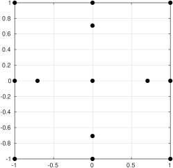
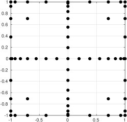
Figure 2: Sparse grid for two parameters of level 2 on the left, level 4 on the centre and level 6 on the right.

Specifically, the set $\mathcal{K}$ is defined as the largest possible one such that the discrete projection is exact for any function spanned by $\{\phi_{\bm{k}}\}_{k\in\mathcal{K}}$, i.e.:

$$\forall\bm{k},\bm{l}\in\mathcal{K},\>\sum_{q=1}^{M}{w^{(q)}\phi_{\bm{k}}(\bm{\xi}^{(q)})\phi_{\bm{l}}(\bm{\xi}^{(q)})}=\begin{dcases*}1&if $\bm{k}=\bm{l}$\\ 0&otherwise\end{dcases*}.$$

In this work, we have opted for an isotropic sparse tensorization of nested Clenshaw–Curtis quadrature rules, where the level $l\in\mathbb{N}$ of the sparse grid is the only parameter controlling the quality of the approximation. As $l$ increases, both the number of nodes $M$ and the multi-index set $\mathcal{K}$ increase.

5.3 Sensitivity analysis

The sensitivity analysis consists in the evaluation of the different contributions of the input parameters on the variance of the solution. This is achieved by the computation of the Sobol indices, defined as the ratio between the partial variance corresponding to the input parameter under investigation $\xi_{i}$, and the total variance of the quantity of interest $X$

$$S_{1,i}:=\frac{\mathbb{V}{\rm ar}(\mathbb{E}(X(\bm{\xi})|\xi_{i}))}{\mathbb{V}{\rm ar}(X(\bm{\xi}))},\qquad\forall 1\leq i\leq N,$$ (20)

where $\mathbb{E}(X(\bm{\xi})|\xi_{i})$ denotes the conditional expected value of $X$ given $\xi_{i}$. The indices $(S_{1,i})_{1\leq i\leq N}$ in (20) are known as principal or first-order Sobol indices and measure the individual contribution of the coefficient $\xi_{i}$ to the variance.

Higher-order Sobol indices measure the effect of the concurrent variation of more variables. For instance, second-order Sobol indices read

$$S_{i,j}:=\frac{\mathbb{V}{\rm ar}(\mathbb{E}(X(\bm{\xi})|\xi_{i},\xi_{j}))}{\mathbb{V}{\rm ar}(X(\bm{\xi}))}-S_{1,i}-S_{1,j},\qquad\forall 1\leq i<j\leq N.$$

Finally, the total Sobol index is obtained as the sum of the indices involving parameter $\xi_{i}$

$$S_{T_{i}}:=1-\frac{\mathbb{V}{\rm ar}(\mathbb{E}(X(\bm{\xi})|\bm{\xi}_{\setminus i}))}{\mathbb{V}{\rm ar}(X(\bm{\xi}))},$$

where the vector $\bm{\xi}_{\setminus i}=\left(\xi_{j\neq i}\right)$ contains all uncertain variables except $\xi_{i}$.

The computation of the Sobol indices results directly from the PC approximation (18) of the variable of interest. Indeed, the partial variances can be explicitly expressed as functions of the spectral modes similarly to the statistical quantities in (19). We refer the reader to [8] for all the details.

6 Numerical examples

In this section, we present two test cases to validate the proposed approach. In both cases we show the reference numerical solution and discuss the uncertainty quantification related to three parameters affected by uncertainty.

Due to the complexity of the problem, all data in the two cases are the same except for the number of fractures in the network. In the first case, presented in Subsection 6.1, a single fracture touching one boundary is considered, while in Subsection 6.2, ten intersecting fractures are considered.

The data for the Darcy problem, the heat equation, and the precipitattion-dissolution process are given in Table 1. Furthermore, we assume that the following three parameters are affected by uncertainty and uniformly distributed with mean and variance given by

$$\eta_{\gamma}\sim\mathcal{U}(2,0.17)\qquad E\sim\mathcal{U}(4,0.35)\qquad\theta^{\rm inflow}\sim\mathcal{U}(1.5,0.11)$$

where $\theta^{\rm inflow}$ denotes the inflow temperature on the bottom boundary. Being the construction of the sparse grids dependent only on the chosen level and the number of uncertain parameters, the number of simulations needed to construct the PC expansion are: 31 runs for level 2, 111 runs for level 3, 351 for level 4, 1023 for and level 5. Once constructed, the evaluation of the PC expansion takes a small fraction of the time used by the full order model to evaluate the solutions for different times and for different values of the uncertain parameters. Hence, we will use the PC expansion as a surrogate model and evaluate its performances and accuracy properties.

$\mu=1$	$g=0$	$\rho_{w}=1$	$k_{\Omega,0}=1$	$\phi_{\Omega,0}=0.2$
$d_{\Omega}=0.1$	$c_{w}=1$	$c_{s}=1$	$\Lambda_{w}=1$	$\Lambda_{s}=0.1$
$j=0$	$\theta_{0}=0$	$\lambda=10\exp(-\frac{E}{\theta})$	$u_{0}=0$	$w_{0}=0.3$
$u_{e}=1$	$p_{\partial\Omega}^{\rm inflow}=1$	$p_{\partial\Omega}^{\rm outflow}=0$	$p_{\partial\gamma}^{\rm inflow}=1$	$p_{\partial\gamma}^{\rm outflow}=0$
$\epsilon_{\gamma,0}=10^{-2}$	$k_{\gamma,0}=10^{2}$	$\kappa_{\gamma,0}=10^{2}$	$f_{\Omega}=0$	$f_{\gamma}=0$
$\theta_{\partial\Omega}^{\rm inflow}=1.5$	$\theta_{\partial\gamma}^{\rm inflow}=1.5$	$u_{\partial\Omega}^{\rm inflow}=2$	$u_{\partial\gamma}^{\rm inflow}=2$	$j_{\gamma}=0$
$d_{\gamma}=0.1$	$\delta_{\gamma}=0.1$	$\eta=0.5$

Table 1: Common data for the advection-reaction problem, examples in Section 6. For $\bullet\in\{k_{\Omega};\phi_{\Omega};\Theta;u;w;\varepsilon_{\gamma};k_{\gamma};\kappa_{\gamma}\}$, the notation $(\bullet)_{0}$ is used for the reference value of the quantity $\bullet$ prescribed as initial condition.

In both cases, we will discuss the convergence properties of the PC expansion by increasing the level of the sparse grid considered, the analysis of the Sobol indices, conditioned variances and covariances for selected solutions and finally the probability distribution functions.

The simulations are developed with the library PorePy, a simulation tool for fractured and deformable porous media written in Python, see [20].

6.1 Single fracture network

Let us consider a domain $\Omega=(0,1)^{2}$ with a single immersed fracture defined by the following vertices: $(0.1,0)$ and $(0.9,0.8)$. The fracture thus touches the bottom boundary of $\Omega$ as depicted in Figure 3. Data and uncertain parameters are reported in the beginning of Section 6.

Figure 3: Domain $\Omega$ and fracture $\gamma$ for the example of Subsection 6.1.

We point out that the fracture is permeable at the beginning of the simulation and due to the solute precipitation its aperture diminishes in time. As a result the effective fracture permeability decreases and until the fracture behaves as a barrier and not any more as a preferential path.

In the following parts, we detail some aspects related to the uncertainty quantification analysis. In Subsection 6.1.1 a convergence study is carried out, in Subsection 6.1.2 we discuss the variances and covariances of the solutions and in Subsection 6.1.3 we introduce the computed probability distribution functions of some of the components of the solutions along the fracture.

The reference solution, corresponding to the average input parameters, is reported in Figure 4, where it is possible to notice the variation of the pressure distribution over time due to the sealing of the fractures and the transport of the solute when the fractures are still highly permeable.

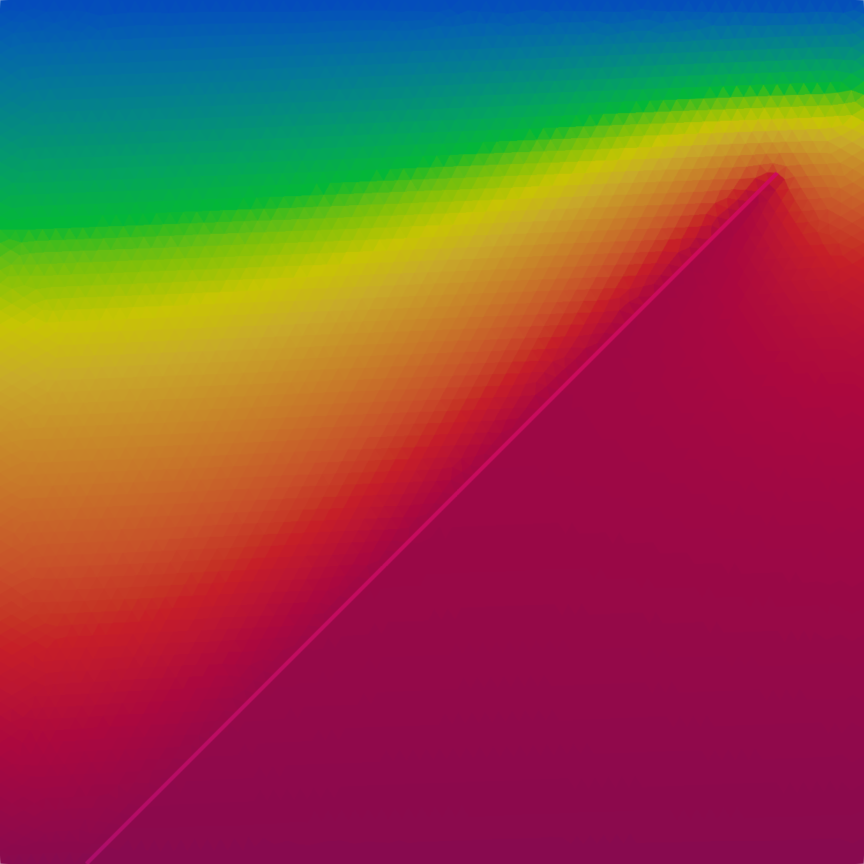
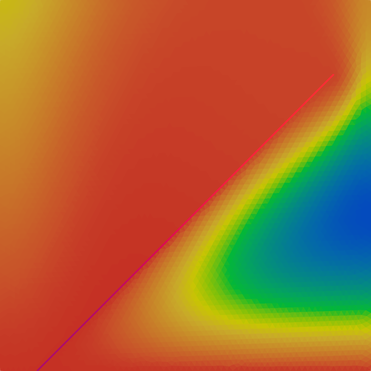
Figure 4: Reference solutions with mean value of the uncertain parameters. On the left pressure at time $t=0.1T$ and on the centre for $t=T$, on the right the solute for $t=0.1T$. Test case of Subsection 6.1.

6.1.1 Convergence

In this part, we discuss the convergence and accuracy properties of the surrogate model built with the PC expansion. In fact, the latter can be used to make fast simulations without the need of running the full order model. Since we are dealing with a time dependent problem, we analyse the PC expansion for two different simulation times: after few time steps $(t=t_{1}=0.1T)$ and at the end of the simulation $(t=T)$.

Figure 5 presents, for both times, the error decay of the computed solutions by increasing the level of the sparse grid. For a smooth relation between uncertain parameters and the solutions, we expect exponential decay of the error with respect to the level, which is the behaviour observed in the figure. Additionally, for $t=t_{1}$ the error computed is much smaller compared to the end of the simulation, showing a temporal dependence on the quality of the PC expansion.

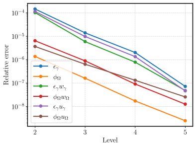
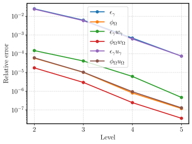
Figure 5: Error convergence for increasing level of the sparse grids, on the left at time $t=0.1T$ and on the right at final time $t=T$. Test case of Subsection 6.1.1.

In Figure 6, we compare the porosity $\phi$ computed with the full order model with the one constructed by the PC expansion and the corresponding relative error. The two solutions are in good agreement for both times and the error is rather low. As before, the latter is smaller at the beginning of the simulation and tends to increase at the end, in particular near the inflow boundary at the bottom of $\Omega$. Moreover, at the beginning of the simulation the fracture is highly permeable and, consequently, we observe also a region in the proximity of $\gamma$ where the error is higher due to stronger geochemical effects.

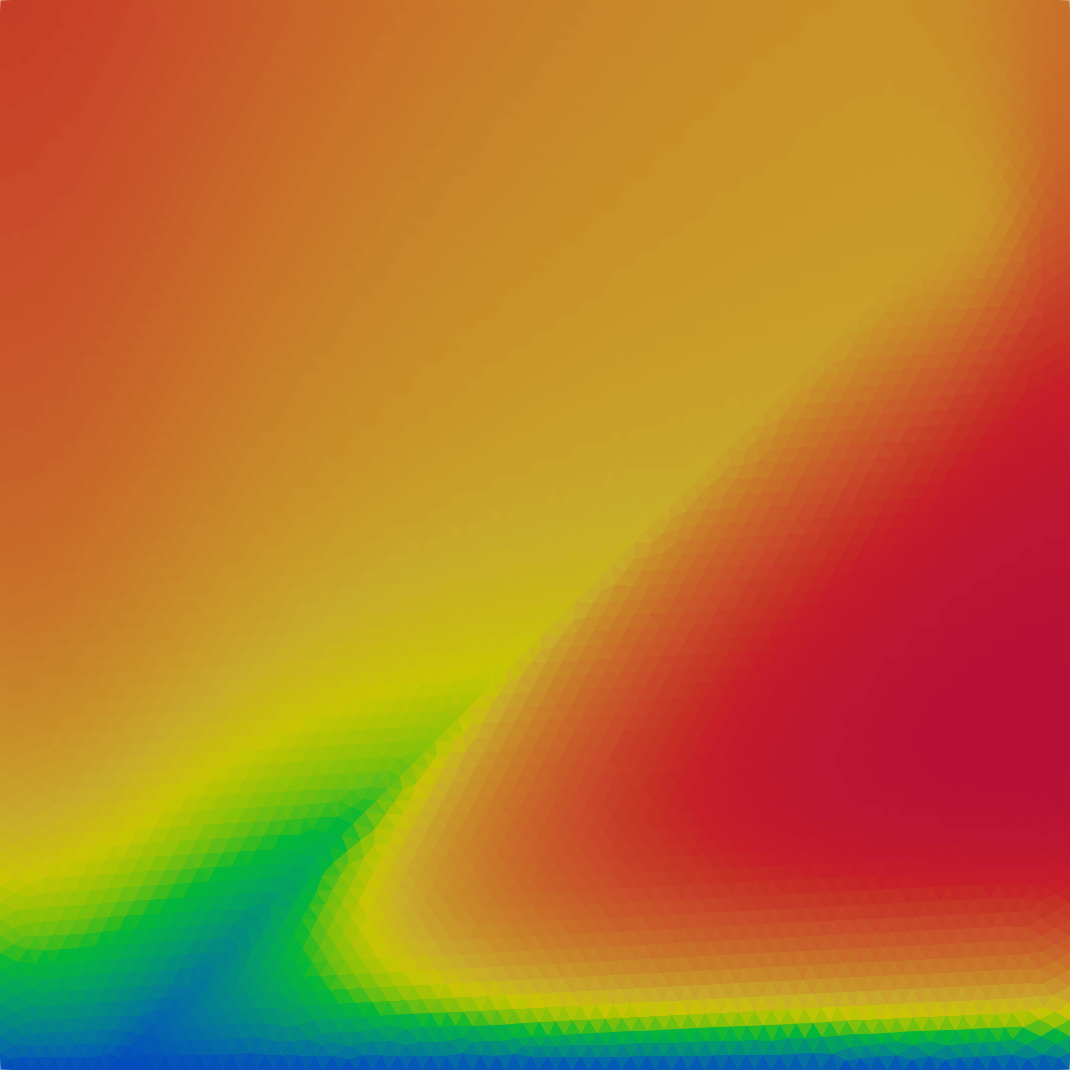
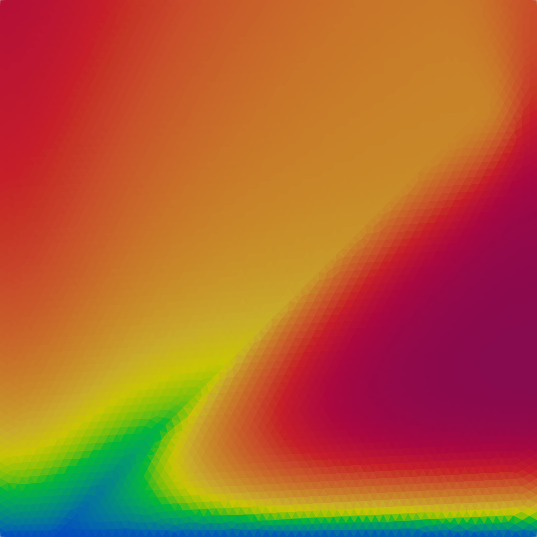
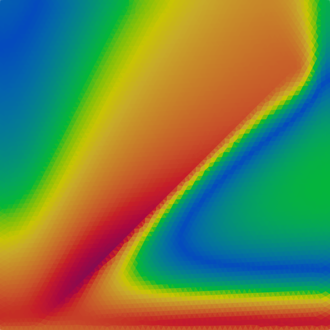
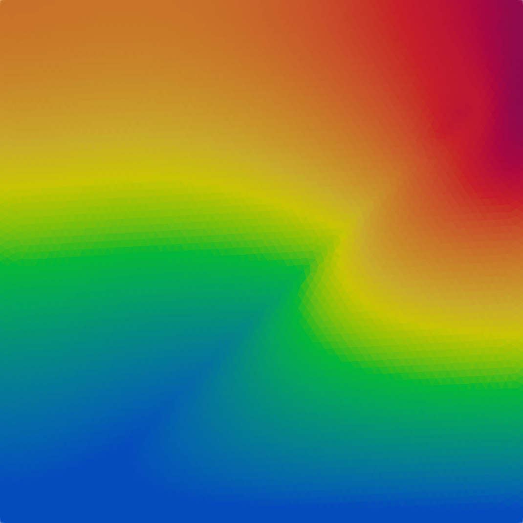
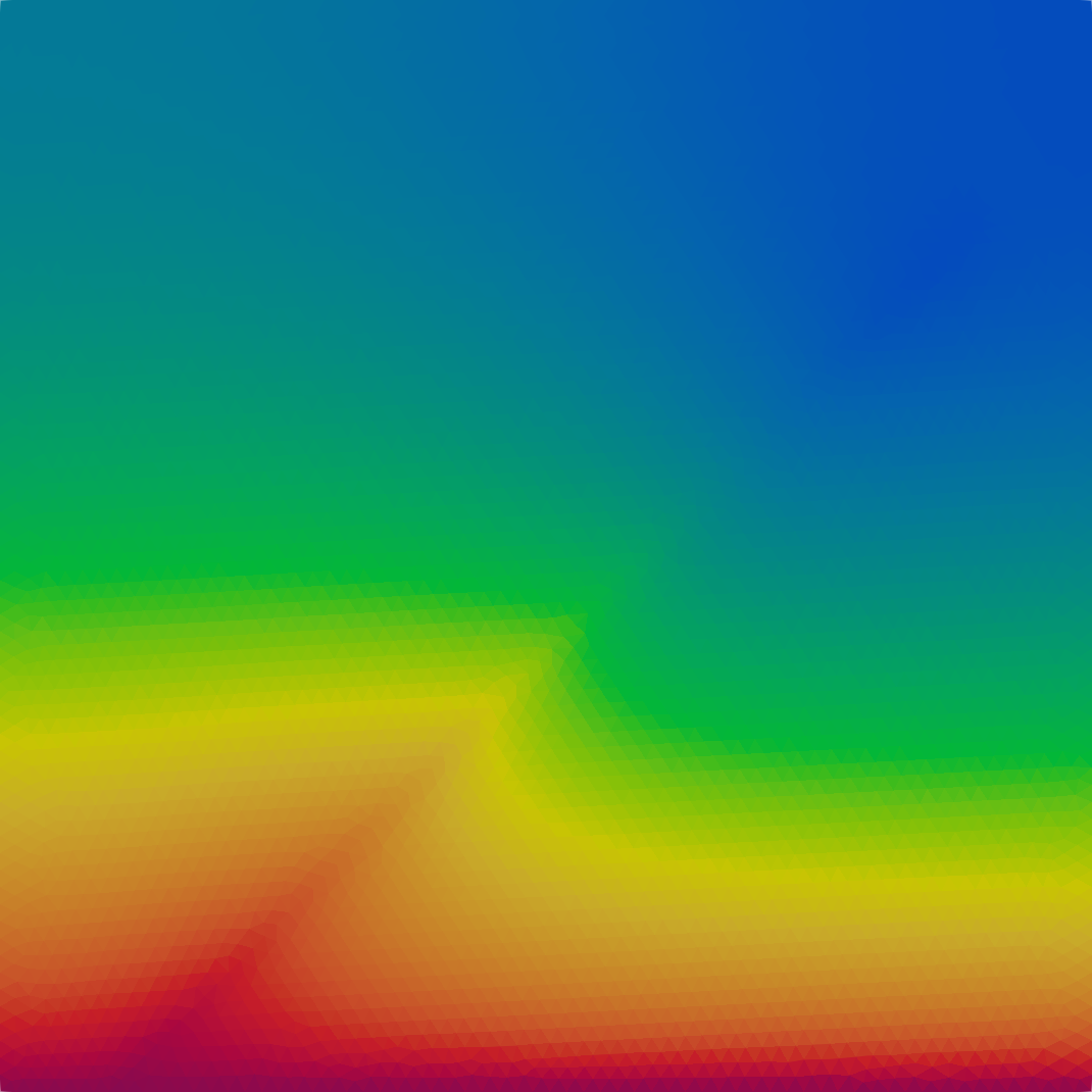
Figure 6: On the left porosity in the media computed with the original model and on the centre with the polynomial chaos expansion, on the right the error between them. On the top at time $t=0.1T$ and on the bottom at final time $t=T$. Test case of Subsection 6.1.1.

Finally, Figure 7 compares some of the variables in the fractures computed with the full order model or reconstructed with the PC expansion. Also in this case, the quality of the latter is high and in good agreement with the reference solution. Moreover, in Figure 7 the green dashed lines represent the solutions obtained for each run to construct the PC expansion and can be useful to visualize the variance of the solution.

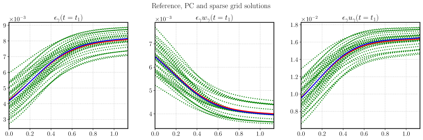
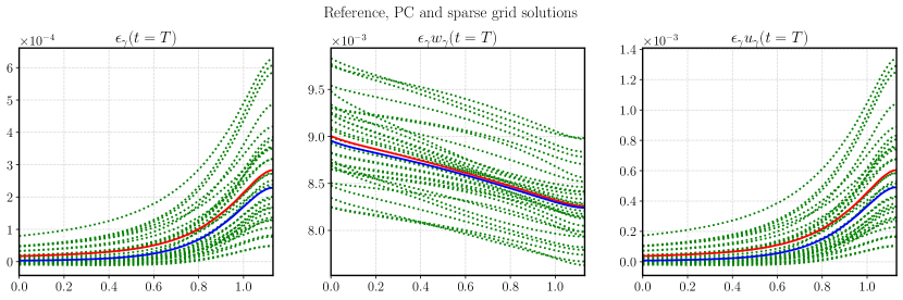
Figure 7: Solutions along $\gamma$: in blue computed with the original model, in red with the polynomial chaos expansion and in green computed by the original model on each sparse grid node (sparse grid level 2). On the top at time $t=0.1T$ and on the bottom at final time $t=T$. Test case of Subsection 6.1.1.

6.1.2 Analysis of variance and correlations

An important factor is the impact on observed variables of the uncertain input data. In Figure 8 we report the Sobol indices for some variables in the fracture for $t=t_{1}$ and $t=T$. We notice that the three variables are influenced in a similar manner by the uncertain data, and the activation energy is the most important factor, followed by the temperature at the inflow boundary. We notice that while the high temperature front penetrates in the domain and in the fracture, the importance of the activation energy over the temperature inflow tends to diminish and the latter becomes more important.

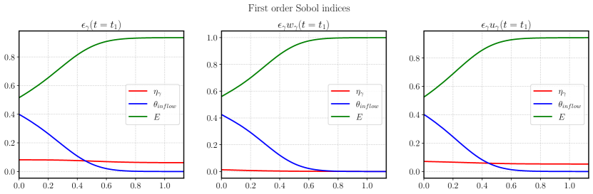
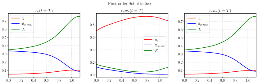
Figure 8: First order Sobol indexes for different unknowns along $\gamma$, on the top at time $t=t_{1}$ and on the bottom at final time $t=T$. The local coordinate of the fracture starts from the bottom boundary. Test case of Subsection 6.1.2.

Note also that the Sobol indices of $\epsilon_{\gamma}w_{\gamma}$ at final time are different from the other two considered variables since $\eta_{\gamma}$ dominates the induced uncertainty of the precipitate.

In Figure 9, we compare the variances of the porosity in the domain $\Omega$ induced by the uncertain data. Depending on the situation, it might be more convenient to consider the Sobol indices instead of the variances in particular when they span different order of magnitudes. The importance of the activation energy over time is rather interesting. In the beginning the fracture is highly permeable and most of the flow is concentrated around the fracture. However, due to the deposition of new material the fracture becomes very low permeable; thus the water flow tends to avoid it and concentrates more in the right part of the domain, where the solute is transported and becomes precipitate altering the porosity. This effect, less evident, can be seen also in the spatial distribution of the Sobol index of $\eta_{\gamma}$. For the temperature, we still notice the permeability change effect coupled with the inflow of higher temperature that speeds up the precipitation process and, as a result, the porosity decay.

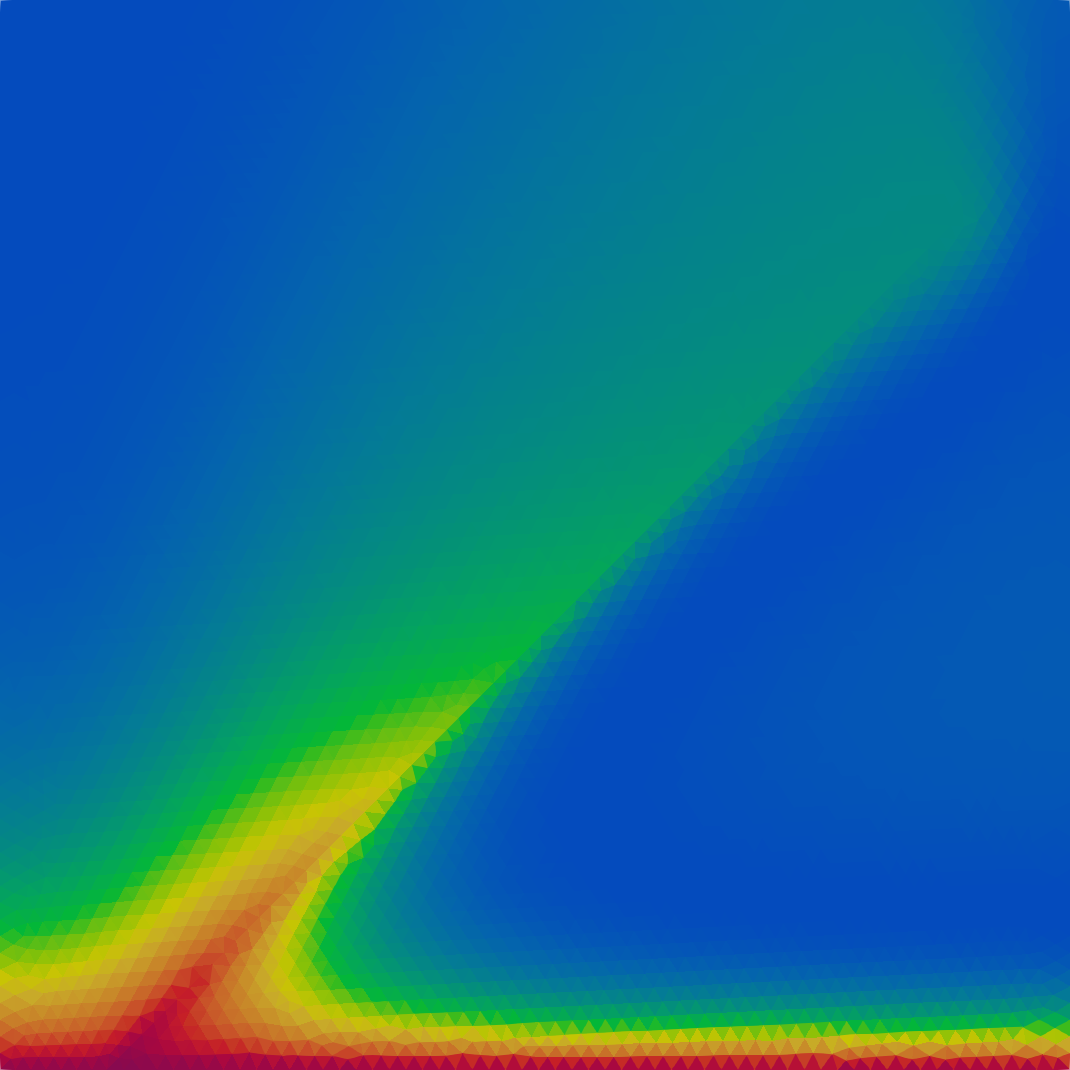
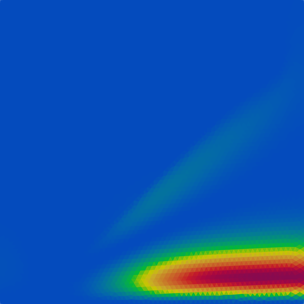
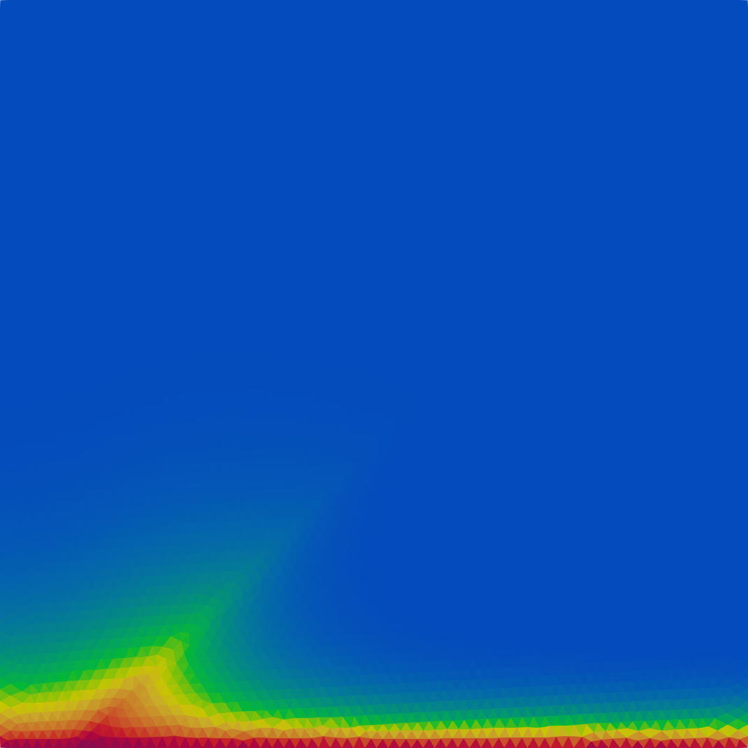
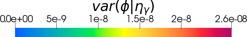
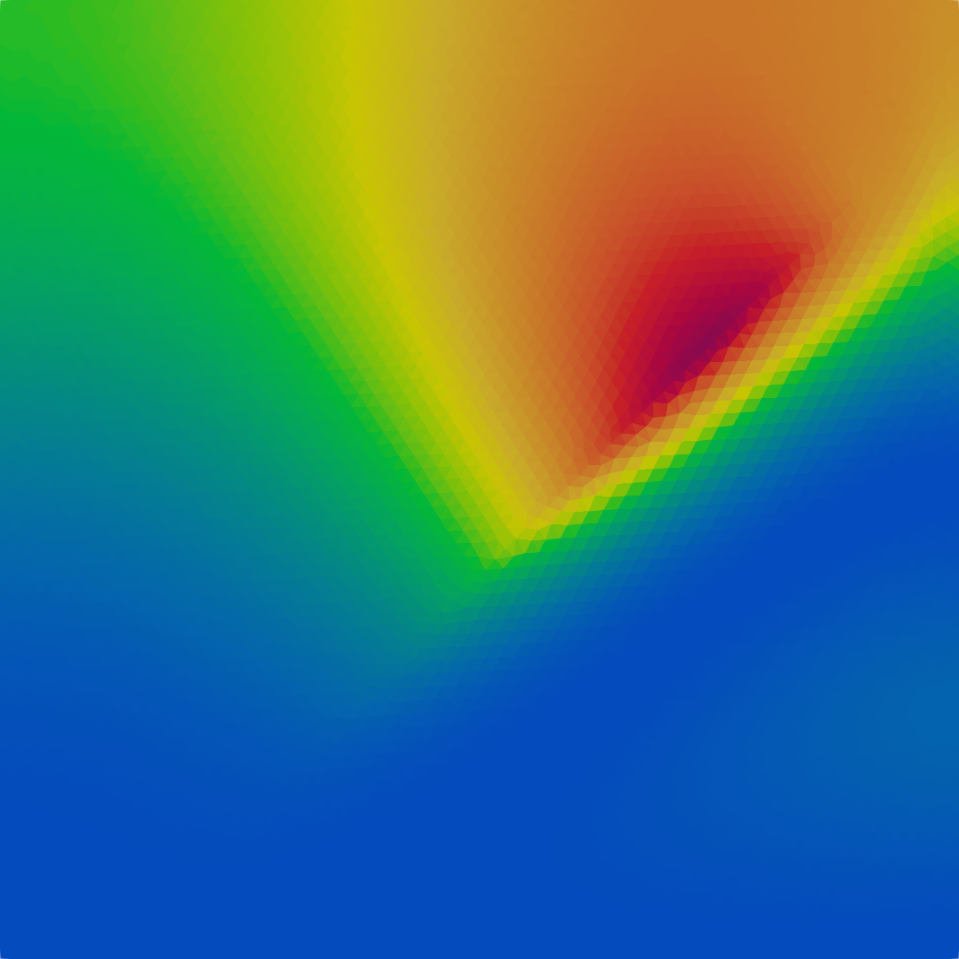
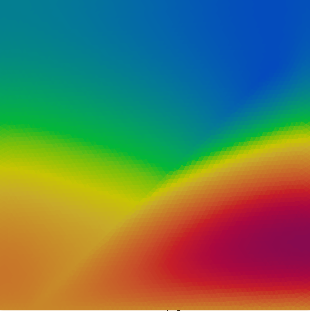
Figure 9: On the left the variance of porosity conditioned to the activation energy $E$, on the centre conditioned with $\eta_{\gamma}$ expansion, and on the right conditioned with the temperature inflow $\theta^{inflow}$. On the top at time $t=0.1T$ and on the bottom at final time $t=T$. Test case of Subsection 6.1.2.

Another important aspect is the interdependency of the output variables, which can be expressed by their covariances. Figure 10 presents this relation between the porosity in the media and several other variables at the two considered times. In the pressure-porosity covariance we observe again the effect of the variation of the fracture behavior in time, fromp permeable to impermeable. For the porosity and $\phi_{\Omega}w_{\Omega}$ we observe a negative correlation, namely if more precipitate is deposited in the porous media, less void space is left, and the porosity diminishes. Finally, the temperature front can be seen in the plot of the covariance between $\phi_{\Omega}$ and $\theta_{\Omega}$, i.e. higher values of the latter tend to facilitate the deposition of solute with concentration higher than the equilibrium. This increases the value of the precipitate and consequently lowers the value of the porosity; conversely, in the top part of the domain the effect is the opposite due to the fact that thermal capacity and conductivity depend on the porosity in a complex way.

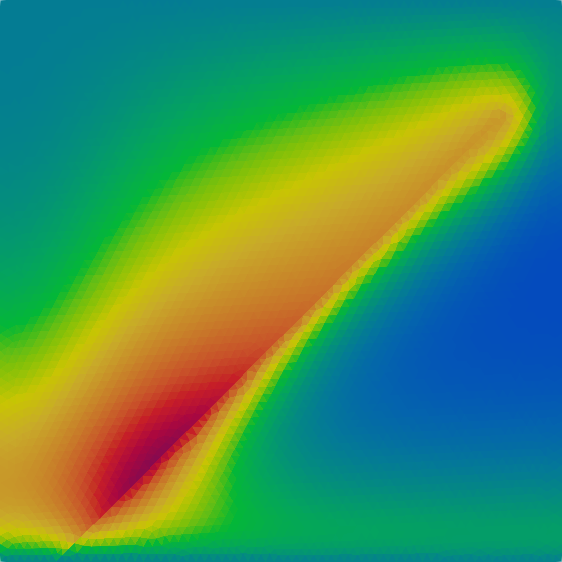
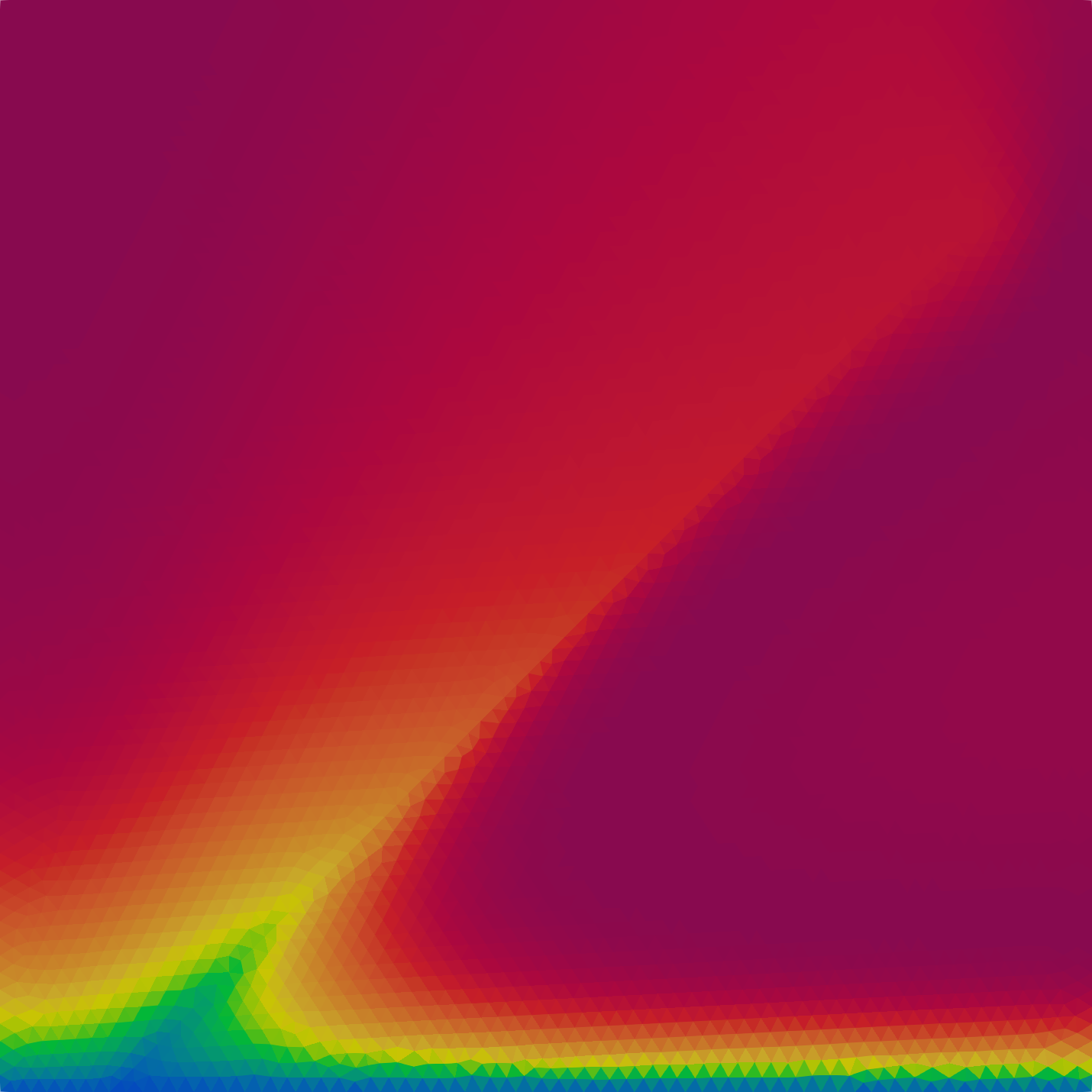
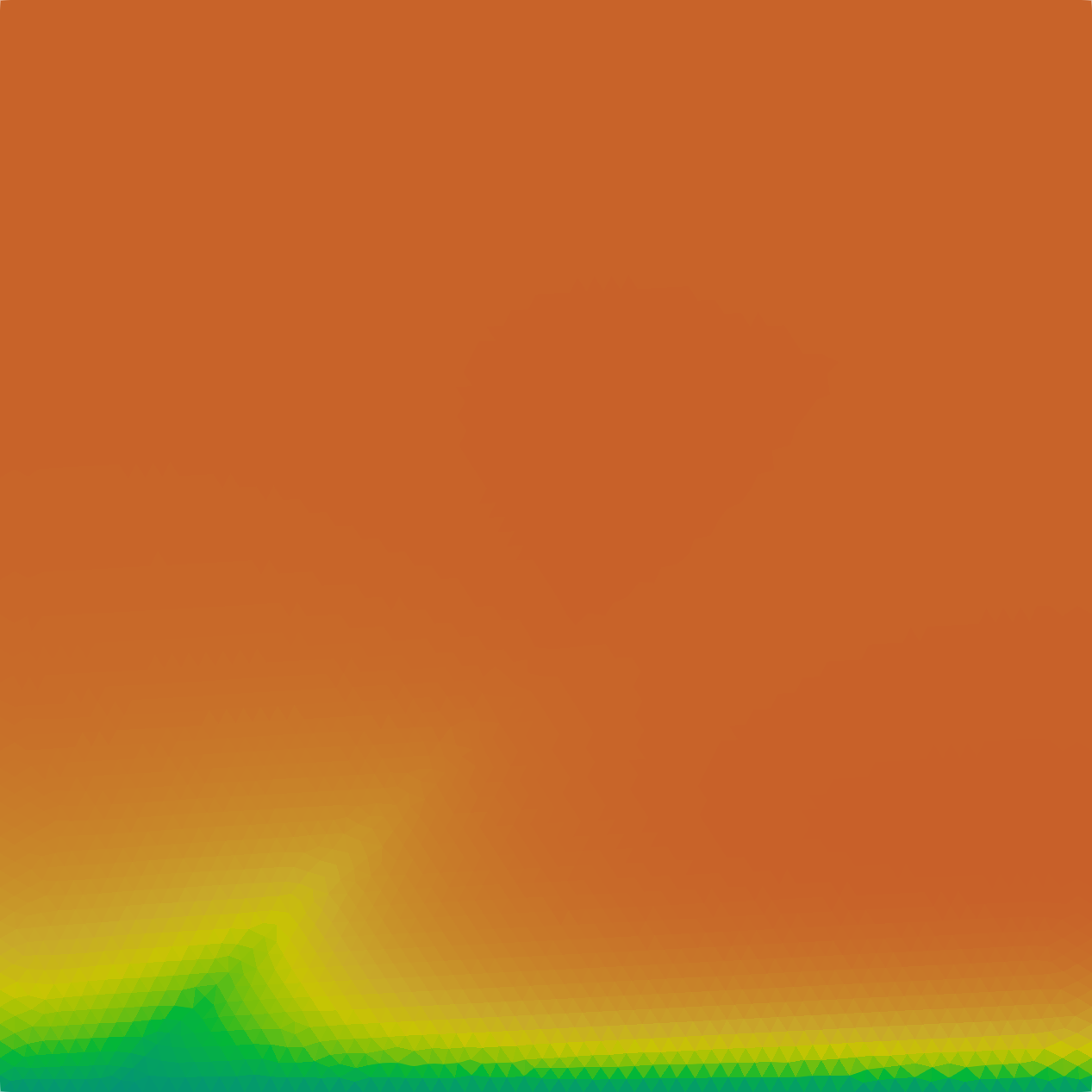
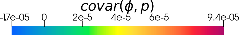
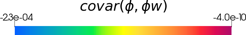
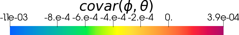
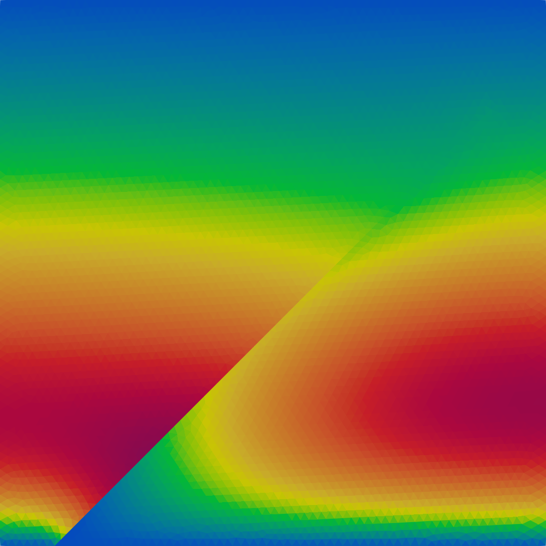
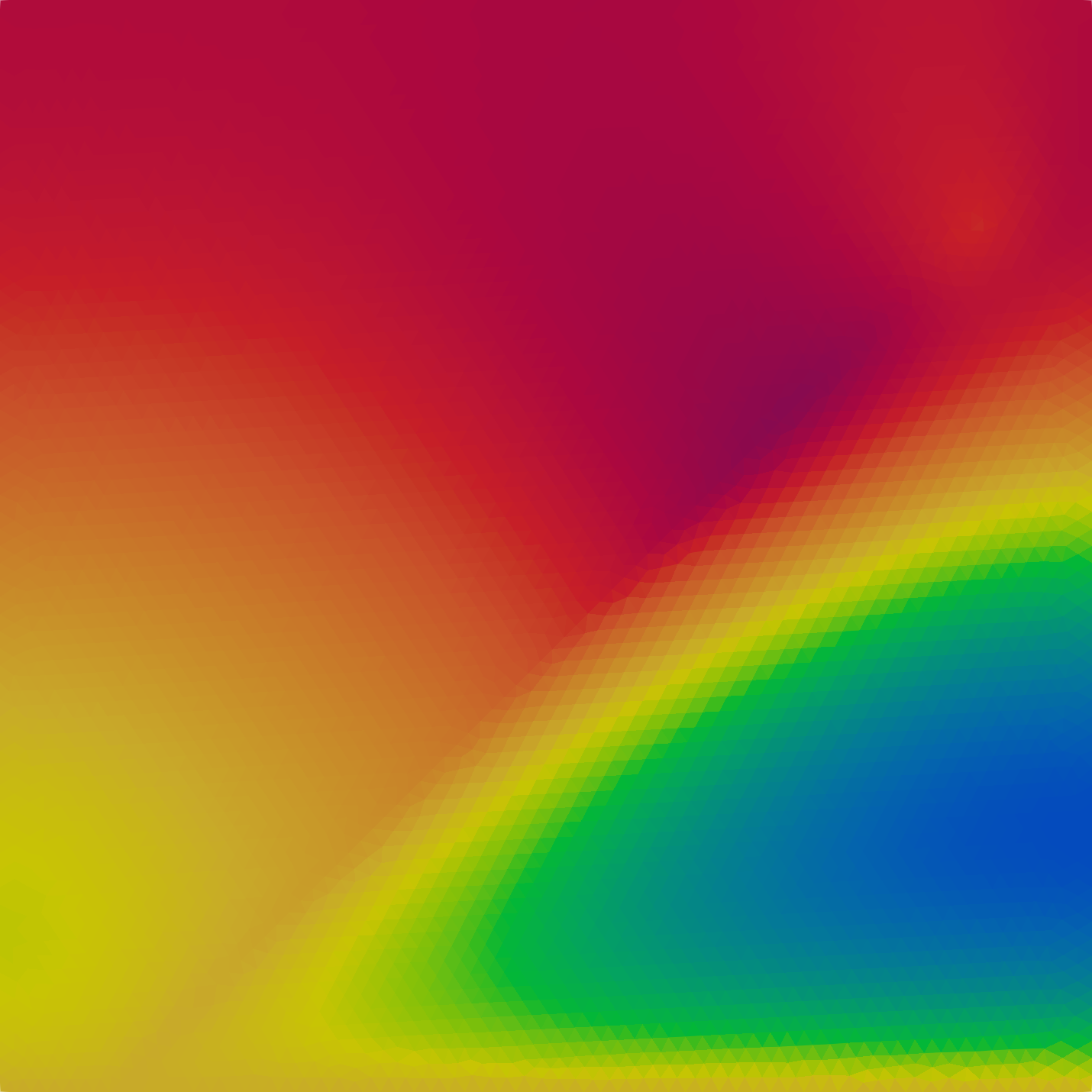
Figure 10: Covariances between different solutions in the porous media. On the top at time $t=0.1T$ and on the bottom at final time $t=T$. Test case of Subsection 6.1.2.

6.1.3 Probability density functions

We consider now the probability density functions (PDFs) of some variables induced by the uncertain data, which are uniformly distributed. Figure 11 shows, for level 2, the distribution of $\epsilon_{\gamma}u_{\gamma}$ at two points along the fracture, and for both times. We notice that at the beginning of the simulation the PDFs are more spread showing a high variability of the considered variable. However, at the end of the simulation the uncertainty tends to become much smaller and the value is more concentrated. Another important aspect is that the PC expansion outcomes might not fulfill physical bounds, in this case we can get negative values of $\epsilon_{\gamma}u_{\gamma}$ which are not correct. The situation improves by considering a higher level of the sparse grid, indeed as represented in Figure 12 this phenomena is not present any more and the PDFs constructed with the PC expansion are in good agreement with the one computed by the full order model.

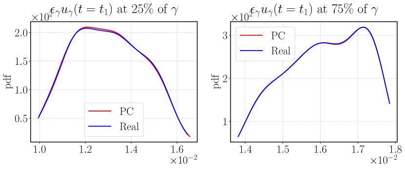
Figure 11: Probability distribution function of $\epsilon_{\gamma}u_{\gamma}$ for level 2 at two points in $\gamma$, on the top at time $t=0.1T$ and on the bottom at final time $t=T$. Test case of Subsection 6.1.3.

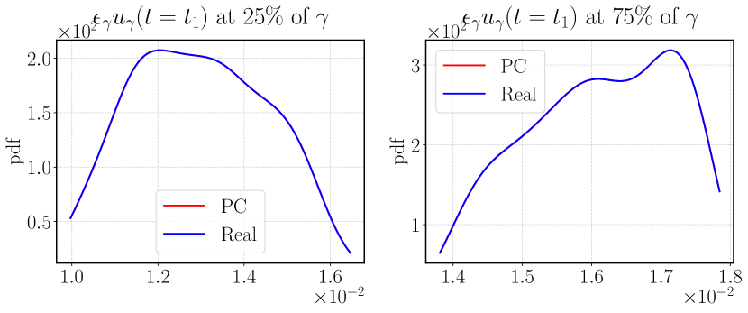
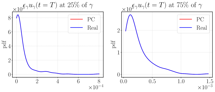
Figure 12: Probability distribution function of $\epsilon_{\gamma}u_{\gamma}$ for level 5 at two points in $\gamma$, on the top at time $t=0.1T$ and on the bottom at final time $t=T$. Test case of Subsection 6.1.3.

6.2 Multiple fractures network

We consider now a test case with a network composed of multiple-fractures. The geometry is given by the Benchmark 3 of [12], where fractures at $t=0$ are now considered all highly permeable with material properties and problem data equal to the previous test case. A graphical representation of the computational domain is given in Figure 14 on the left. Fractures $\gamma_{3}$ and $\gamma_{8}$ will be considered later for a specific analysis.

Some quantities from the reference numerical solution are reported in Figure 13, where it is possible to notice the variation of the pressure distribution over time due to the sealing of the fractures and the transport of the solute when the fractures are still highly permeable.

Figure 13: Reference solutions with mean value of the uncertain parameters. On the left pressure at time $t=0.1T$ and on the centre for $t=T$, on the right the solute for $t=0.1T$. Test case of Subsection 6.2.

6.2.1 Convergence

We discuss now the convergence properties of the PC expansion. On the right of Figure 14, we plot the error decay for increasing sparse grid level for multiple variables. Also in this case, the exponential decay expected is confirmed for all the variables.

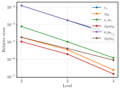
Figure 14: On the right the computational domain with boundary conditions and on the left the error convergence for increasing level of the sparse grids. Test case of Subsection 6.2.1.

In Figure 15 we compare the porosity computed by the differential model with the one computed by the PC expansion. On the right we also represent the relative error. The two solutions are in good agreement with a maximum error of $13\%$ confined at the bottom of the domain, the error is much smaller in the other parts being of the order of $5\%$ or less. The surrogate model provided by the PC expansion gives a satisfactory result at (almost) no additional computational cost.

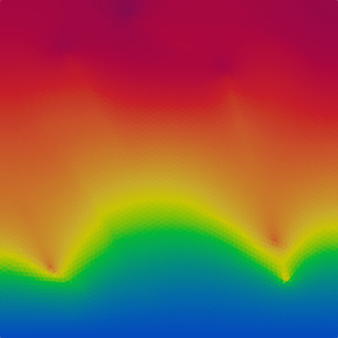
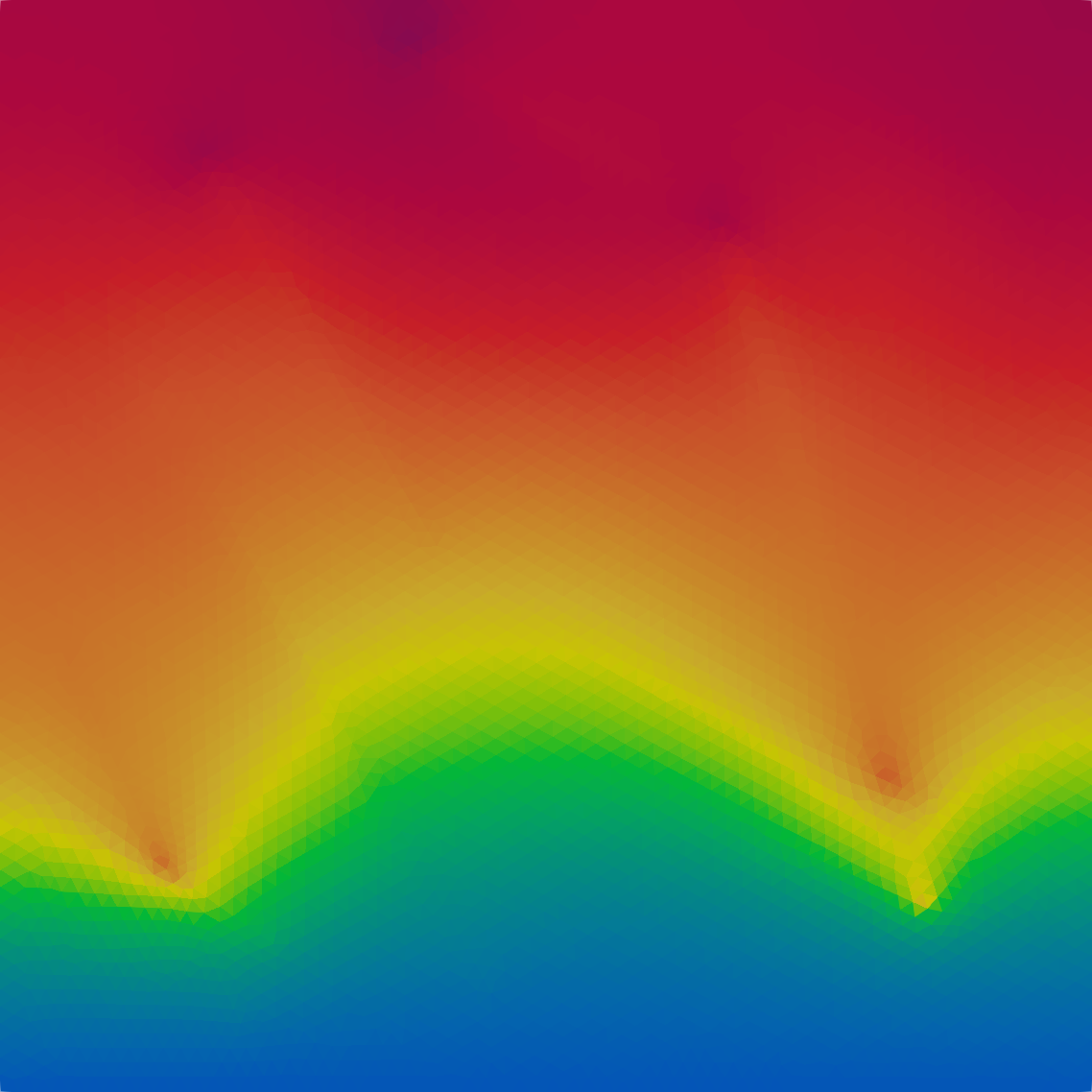
Figure 15: On the left porosity in the media computed with the original model and on the centre with the polynomial chaos expansion, on the right the error between them. Test case of Subsection 6.2.1.

Figure 16 compares some of the variables along the two fractures $\gamma_{3}$ and $\gamma_{8}$ computed by the full order model and by the PC expansion. Also in the fractures, we observe a high quality for the solutions computed with the PC expansion even for $\gamma_{8}$ that has two intersections with other fractures. The jump across the intersection is properly captured, confirming also in this case that the surrogate model from the PC expansion yields a good approximation of the solutions.

Figure 16: Solutions along two $\gamma_{i}$ and in blue computed with the original model, in red with the polynomial chaos expansion and in green computed by the original model on each sparse grid node. On the top $\gamma_{3}$ and on the bottom for $\gamma_{8}$. Level considered 2. Test case of Subsection 6.2.1.

6.2.2 Analysis of variance and correlations

In this section, we present and analyze the impact of the uncertainty on some of the computed variables. In particular, Figure 17 shows the Sobol indices for some of the variables of interest in the fractures $\gamma_{3}$ and $\gamma_{8}$. Since $\gamma_{3}$ is closer to the inflow boundary than $\gamma_{8}$, the associated Sobol indices behave similarly with respect to the ones of the previous test case. The effect of the inflow is more evident at the lowest tip of the fracture $\gamma_{3}$ with increased impact of $\theta^{\mathrm{inflow}}$ for $\epsilon_{\gamma}$ and $\epsilon_{\gamma}u_{\gamma}$ compared to the other variables. For $\epsilon_{\gamma}w_{\gamma}$ the relation expressed by the Sobol index is less clear. Since fracture $\gamma_{8}$ is more distant form the inflow boundary, the high temperature front at the end of the simulation does not fully reach it. Some effect are still visible since warmer water has been transported by the fractures, especially for $\epsilon_{\gamma}w_{\gamma}$ where the activation energy $E$ becomes less important than $\eta_{\gamma}$ compared with the other two variables under investigation.

Figure 17: First order Sobol index for different solutions along two $\gamma_{i}$. On the top $\gamma_{3}$ and on the bottom for $\gamma_{8}$. Test case of Subsection 6.2.2.

In Figure 18 we present the partial variances of the porosity with respect to the uncertain data at final simulation time. We notice a small impact of $\eta_{\gamma}$, and a much more significant relevance of $E$ and $\theta^{inflow}$. Note that the effect of these two uncertain parameters on reaction speed is opposite. Moreover, we notice that, on the bottom of the domain, the effect of the temperature is more pronounced since it is close to the inflow boundary, while for the activation energy $E$ the impact is more predominant away from the inflow and close to the fractures. This can be motivated by the fact that the water and solute get more channelized into the fractures and transported upward. Since the fractures do not touch the outflow boundary, the solute flows again into the rock matrix and then alters the value of the porosity by creating more precipitate.

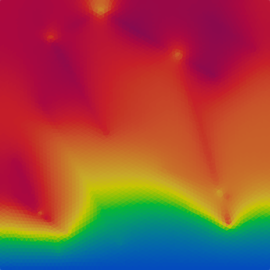
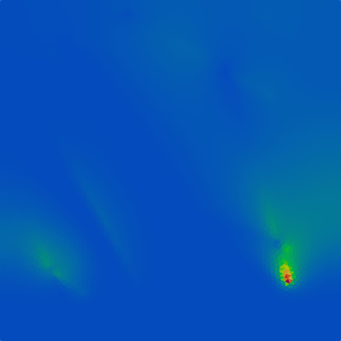
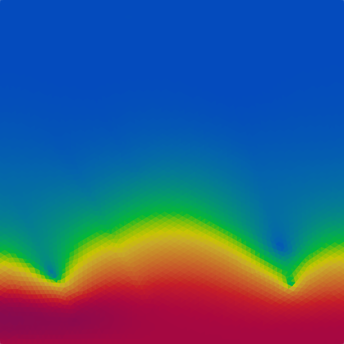
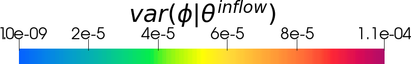
Figure 18: On the left the variance of porosity conditioned to the activation energy $E$, on the centre conditioned with $\eta_{\gamma}$ expansion, and on the right conditioned with the temperature inflow $\theta^{inflow}$. Test case of Subsection 6.2.2.

The covariances between some of the computed variables are reported in Figure 19. The correlation between $\phi_{\Omega}$ and $\theta_{\Omega}$ is expected: below the warm water front, the increased temperature facilitates the chemical reaction and thus lowers the porosity; above the front, the solute is lower than the equilibrium value and the temperature is lower, hence precipitation may not occur once fractures have been sealed and stopped supplying reactant to the upper part of the domain. The correlation between $\phi_{\Omega}u_{\Omega}$ and $\phi_{\Omega}w_{\Omega}$ is not included here since they are, as expected, equal to -1 in the whole domain. The same applies for $\epsilon_{\gamma}u_{\gamma}$ and $\epsilon_{\gamma}w_{\gamma}$.

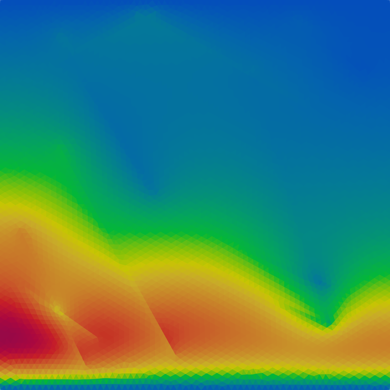
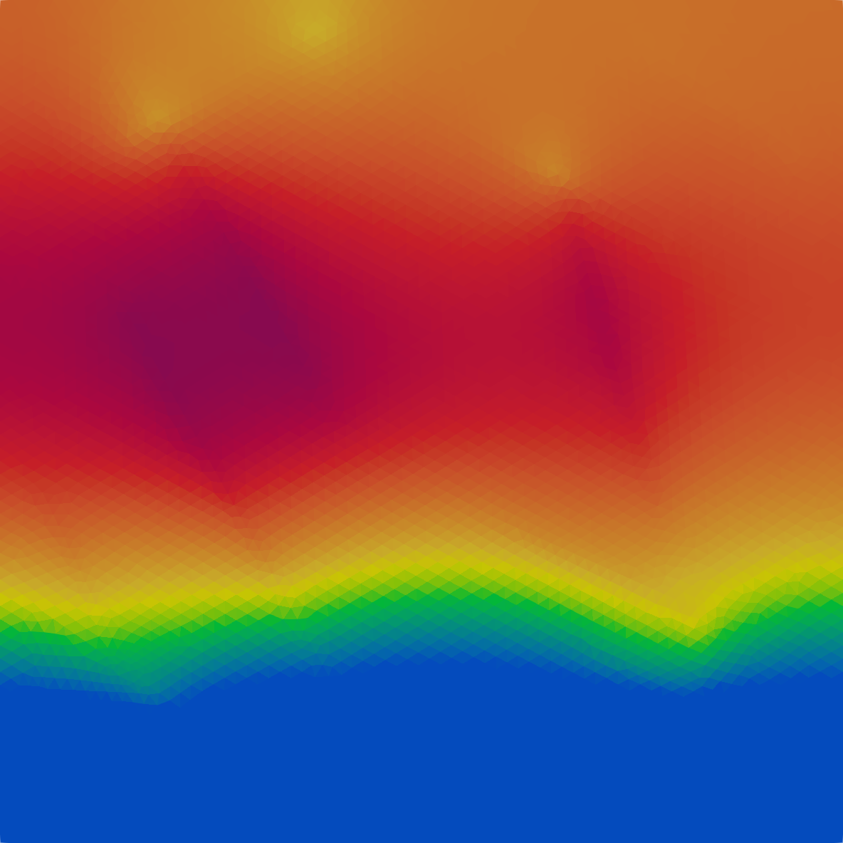
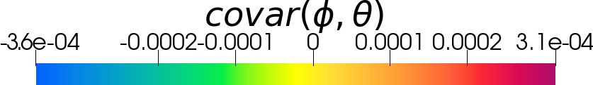
Figure 19: Covariances between different solutions in the porous media. Test case of Subsection 6.2.2.

6.2.3 Probability density functions

Finally, we present the PDFs of some of the variables at 25% and 75% of fractures $\gamma_{3}$ and $\gamma_{8}$ for level 2 of the sparse grid. We notice a phenomenon similar to the one observed in the previous test case. For $\gamma_{3}$ we might obtain unphysical values of $\epsilon_{\gamma}u_{\gamma}$ when the PDF is computed by the PC expansion. This issue does not appear for $\gamma_{8}$, since it is further from the inflow and, as a consequence, is less subject to the uncertainty. In both cases the probability distribution functions computed with the original model and with the PC expansion are quite similar.

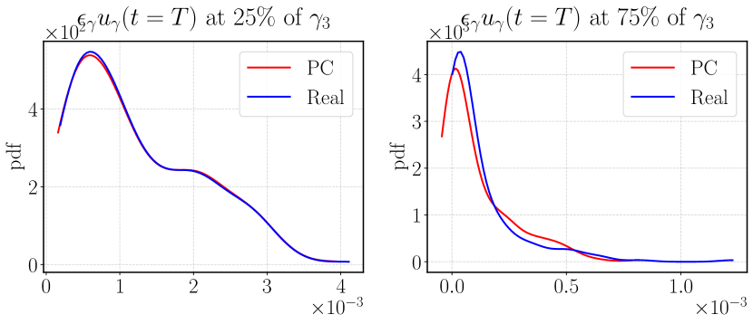
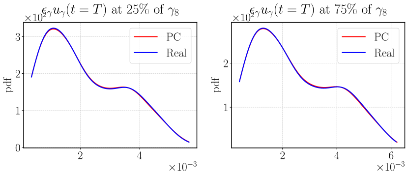
Figure 20: Probability distribution function of $\epsilon_{\gamma_{i}}u_{\gamma_{i}}$ for level 2 at two points in $\gamma_{i}$. On the top $\gamma_{3}$ and on the bottom for $\gamma_{8}$. Level considered 2. Test case of Subsection 6.2.3.

7 Conclusions

In this work we have presented a mathematical model to describe the evolution in time of reactive transport in fractured porous media. We have adopted a simplified model, where only one solute and one precipitate are involved in the chemical reactions. In several meaningful applications, the chemical processes can be triggered and accelerated by high temperatures, thus we have included in the model also an additional equation to model the thermal effects. The solute, transported by a liquid, might form precipitate and alter the porosity in the media, forming a fully coupled and non-linear system. In order to obtain a more realistic approximation of the physical process, we have considered a mixed-dimensional model for the fractures where the latter are represented as object of lower dimension. We have introduced appropriate equations and derived coupling conditions with the surrounding porous media. Additionally, we have applied a splitting strategy to numerically solve the problem by using standard discretization schemes.

In a real scenario, several parameters might be affected by uncertainty. To quantify their effect on the system, we have considered a polynomial chaos expansion constructed by resorting to spectral projection methods on sparse grids. This strategy proved to be very effective, since it provides high quality approximations at low computational cost. Indeed, a limited amount of simulations are needed to construct a surrogate model which can then be used to perform multiple-simulations. Moreover, from the PC expansion one can easily compute useful statistical quantities such as partial variances and Sobol indexes to investigate the impact of input parameters on the model unknowns and gain insight into the complex model couplings. This technique has been applied to two numerical examples by increasing the geometrical complexity of the fracture network. The results obtained showed the validity of the proposed approach.

Fundings

Michele Botti acknowledges funding from the European Union’s Horizon 2020 research and innovation programme under the Marie Skłodowska-Curie grant agreement No. 896616 “PDGeoFF”. All authors are members of the INdAM Research group GNCS.

Conflict of interest

The authors have no conflicts of interest to declare that are relevant to the content of this article.

Authors’ contribution

Michele Botti has provided the uncertainty quantification tools used in the work; Alessio Fumagalli and Anna Scotti have devised the mathematical models and all authors contributed to the critical discussion of the test cases, as well as to the writing of the manuscript. Moreover, they all have read and approved the final version.

Availability of data and material

The source code at the basis of the numerical tests is available at https://github.com/pmgbergen/porepy.

References

- [1] Elyes Ahmed, Alessio Fumagalli, and Ana Budiša. A multiscale flux basis for mortar mixed discretizations of reduced Darcy-Forchheimer fracture models. Computer Methods in Applied Mechanics and Engineering, 354:16–36, 2019.
- [2] I. Babuška and P. Chatzipantelidis. On solving elliptic stochastic partial differential equations. Comput. Methods Appl. Mech. Engrg., 191(37):4093–4122, 2002.
- [3] Inga Berre, Florian Doster, and Eirik Keilegavlen. Flow in fractured porous media: A review of conceptual models and discretization approaches. Transport in Porous Media, 130(1):215–236, 2019.
- [4] M. Botti, D. A. Di Pietro, O. Le Maître, and P. Sochala. Numerical approximation of poroelasticity with random coefficients using Polynomial Chaos and Hybrid High-Order methods. Comput. Methods Appl. Mech. Eng., 361, April 2020.
- [5] Florent Chave, Daniele A. Di Pietro, and Luca Formaggia. A hybrid high-order method for darcy flows in fractured porous media. SIAM Journal on Scientific Computing, 40(2):A1063–A1094, 2018.
- [6] P. R. Conrad and Y. M. Marzouk. Adaptive Smolyak pseudospectral approximations. SIAM J. Sci. Comp., 35(6):A2643–A2670, 2013.
- [7] P. G. Constantine, M. S. Eldred, and E. T. Phipps. Sparse pseudospectral approximation method. Comput. Methods Appl. Mech. Engrg., 229:1–12, 2012.
- [8] T. Crestaux, O. Le Maître, and J.-M. Martinez. Polynomial chaos expansion for sensitivity analysis. Reliability Engineering & System Safety, 94(7):1161 – 1172, 2009. Special Issue on Sensitivity Analysis.
- [9] Jérôme Droniou. Finite volume scheme for diffusion equations: Introduction to and review of modern methods, Apr 2013. working paper or preprint.
- [10] Robert Eymard, Thierry Gallouët, and Raphaèle Herbin. Finite volume methods. In P. G. Ciarlet and J. L. Lions, editors, Solution of Equation in (Part 3), Techniques of Scientific Computing (Part 3), volume 7 of Handbook of Numerical Analysis, pages 713–1018. Elsevier, 2000.
- [11] Isabelle Faille, Eric Flauraud, Frédéric Nataf, Sylvie Pégaz-Fiornet, Frédéric Schneider, and Françoise Willien. A New Fault Model in Geological Basin Modelling. Application of Finite Volume Scheme and Domain Decomposition Methods. In Finite volumes for complex applications, III (Porquerolles, 2002), pages 529–536. Hermes Sci. Publ., Paris, 2002.
- [12] Bernd Flemisch, Inga Berre, Wietse Boon, Alessio Fumagalli, Nicolas Schwenck, Anna Scotti, Ivar Stefansson, and Alexandru Tatomir. Benchmarks for single-phase flow in fractured porous media. Advances in Water Resources, 111:239–258, Januray 2018.
- [13] Luca Formaggia, Alessio Fumagalli, Anna Scotti, and Paolo Ruffo. A reduced model for Darcy’s problem in networks of fractures. ESAIM: Mathematical Modelling and Numerical Analysis, 48:1089–1116, 7 2014.
- [14] Alessio Fumagalli and Anna Scotti. Reactive flow in fractured porous media. In Finite Volumes for Complex Applications IX proceedings. Springer, 2020. Accepted.
- [15] Alessio Fumagalli and Anna Scotti. A mathematical model for thermal single-phase flow and reactive transport in fractured porous media. Journal of Computational Physics, 434, 2021.
- [16] T. Gerstner and M. Griebel. Dimension-adaptive tensor-product quadrature. Computing, 71(1):65–87, 2003.
- [17] R. G. Ghanem and S. Dham. Stochastic finite element analysis for multiphase flow in heterogeneous porous media. Transport in Porous Media, 32(3):239–262, 1998.
- [18] R. G. Ghanem and S. D. Spanos. Stochastic Finite Elements: a Spectral Approach. Springer Verlag, 1991.
- [19] Jérôme Jaffré, Mokhles Mnejja, and Jean E. Roberts. A discrete fracture model for two-phase flow with matrix-fracture interaction. Procedia Computer Science, 4:967–973, 2011.
- [20] Eirik Keilegavlen, Runar Berge, Alessio Fumagalli, Michele Starnoni, Ivar Stefansson, Jhabriel Varela, and Inga Berre. Porepy: An open-source software for simulation of multiphysics processes in fractured porous media. Computational Geosciences, 2020.
- [21] O. Le Maître, M. T. Reagan, H. N. Najm, R. G. Ghanem, and O. M. Knio. A stochastic projection method for fluid flow II.: Random process. J. Comput. Phys., 181(1):9–44, 2002.
- [22] O. P. Le Maître and O. M. Knio. Spectral Methods for Uncertainty Quantification. Scientific Computation. Springer, 2010.
- [23] Florence T. Ling, Dan A. Plattenberger, Catherine A. Peters, and Andres F. Clarens. Sealing porous media through calcium silicate reactions with co2 to enhance the security of geologic carbon sequestration. Environmental Engineering Science, 38(3):127–142, 2021.
- [24] Vincent Martin, Jérôme Jaffré, and Jean Elisabeth Roberts. Modeling Fractures and Barriers as Interfaces for Flow in Porous Media. SIAM J. Sci. Comput., 26(5):1667–1691, 2005.
- [25] H. G. Matthies and A. Keese. Galerkin methods for linear and nonlinear elliptic stochastic partial differential equations. Comput. Methods Appl. Mech. Engrg., 194(12-16):1295–1331, 2005.
- [26] Jan Martin Nordbotten, Wietse Boon, Alessio Fumagalli, and Eirik Keilegavlen. Unified approach to discretization of flow in fractured porous media. Computational Geosciences, 23(2):225–237, 2019.
- [27] Florin Adrian Radu, Iuliu Sorin Pop, and Sabine Attinger. Analysis of an Euler implicit - mixed finite element scheme for reactive solute transport in porous media. Numer. Methods Part. Differ. Equat., 26:320–344, 2010.
- [28] Tor Harald Sandve, Inga Berre, and Jan Martin Nordbotten. An efficient multi-point flux approximation method for Discrete Fracture-Matrix simulations. Journal of Computational Physics, 231(9):3784–3800, 2012.
- [29] S.A. Smolyak. Quadrature and interpolation formulas for tensor products of certain classes of functions. Dokl. Akad. Nauk SSSR, 4(240-243):123, 1963.
- [30] N. Wiener. The Homogeneous Chaos. Amer. J. Math., 60:897–936, 1938.