Demonstration of multi-time quantum statistics without measurement back-action

Abstract

It is challenging to obtain quantum statistics of multiple time points due to the principle of quantum mechanics that a measurement disturbs the quantum state. We propose an ancilla-assisted measurement scheme that does not suffer from the measurement-induced back-action and experimentally demonstrate it using dual-species trapped ions. By ensemble averaging the ancilla-measurement outcomes with properly chosen weights, quantum statistics, such as quantum correlation functions and quasi-probability distributions can be reconstructed. We employ ${}^{171}\rm{Yb}^{+}$-${}^{138}\rm{Ba}^{+}$ ions as the system and the ancilla to perform multi-time measurements that consist of repeated initialization and detection of the ancilla state without effecting the system state. The two- and three-time quantum correlation functions and quasi-probability distributions are clearly revealed from experimental data. We successfully verify that the marginal distribution is unaffected by the measurement at each time and identify the nonclassicality of the reconstructed distribution. Our scheme can be applied for any $N$-time measurements of a general quantum process, which will be an essential tool for exploring properties of various quantum systems.

A striking difference between quantum and classical statistics arises as there exist observables in a quantum mechanics that cannot be precisely determined simultaneously. Correlations between these incompatible observables do not follow the description of classical joint probability distributions but can be explained by introducing quasi-probability distributions (QPDs), which allows negative Wigner (1932); Margenau and Hill (1961) or even non-real values Kirkwood (1933); Dirac (1945). Such nonclassical features of QPDs have been widely studied in the fields of quantum foundations BELL (1966); Leggett and Garg (1985); Feynman (1987) and thermodynamics Allahverdyan (2014); Perarnau-Llobet et al. (2017); Yunger Halpern (2017); Lostaglio (2018); Levy and Lostaglio (2020); Kwon and Kim (2019), as well as being considered as a useful resource for quantum computing Veitch et al. (2012); Mari and Eisert (2012); Howard et al. (2014); Pashayan et al. (2015); Rahimi-Keshari et al. (2016) and metrology Kwon et al. (2019); Arvidsson-Shukur et al. (2020); Lostaglio (2020). At the same time, quantum correlation functions and QPDs serve as essential tools for exploring both static and dynamic properties of various quantum systems Kubo (1957); Mandel and Wolf (1995); Gardiner et al. (2004); Clerk et al. (2010); Krumm et al. (2016); Yunger Halpern et al. (2018); Dowling et al. (2021).

Meanwhile, accessing the quantum statistics in experiments is way more challenging than the classical system. Quantum theory prohibits one from directly obtaining the statistics of incompatible observables as a fundamental trade-off relation holds between information gain and measurement-induced disturbance Groenewold (1971); Fuchs and Peres (1996); Ozawa (2003); Buscemi et al. (2014); Fan et al. (2015); Lee et al. (2021); Hong et al. (2022). In particular, projection measurements are not sufficient to fully capture the quantum nature as all the off-diagonal elements are washed out after the measurement and can not contribute to the subsequent measurement statistics. To detour this problem, various indirect methods to obtain quantum correlation functions and QPDs have been theoretically proposed Buhrman et al. (2001); Somma et al. (2002); Johansen (2007); Buscemi et al. (2013); Pedernales et al. (2014); Perarnau-Llobet et al. (2017) and experimentally demonstrated Souza et al. (2011); Piacentini et al. (2016); Xin et al. (2017); Ringbauer et al. (2018); Wu et al. (2019); Del Re et al. (2022). While most of these approaches focus on quantum statics of two-time points, only a few experimental realizations of quantum correlation functions beyond two-time points are reported Xin et al. (2017); Ringbauer et al. (2018).

In this Letter, we propose and experimentally verify that quantum statistics of multiple time points can be reconstructed from ancilla-assisted measurements. Remarkably, the reconstructed quantum statistics do not suffer back-action from the measurement-induced disturbance. To this end, we interact the system with an ancilla state at each time followed by the ancilla measurement with respect to a certain basis set. The quantum statistics is then reconstructed by taking an ensemble average of the sequential measurement outcomes with properly weights. By increasing the number of the ancilla measurement bases, richer quantum statistics, such as quantum correlation function and QPDs, can be obtained.

Our approach has several advantages: (i) the measurement scheme is constructed independent of the system’s dynamics, (ii) the protocol does not require preparing multiple copies of quantum states at the same time, and (iii) coherence between the system and ancilla states is required to be maintained only during a short interaction time. These advantages make the proposed scheme easier to be applied to any multi-time measurements with a longer time scale. On the other hand, the ancilla state should be measured and used repeatedly without affecting the system state. Such in-circuit detection (ICD) and in-circuit initialization (ICI) of the ancilla are demanded for experimental realization of the scheme.

In trapped-ion systems, ICD and ICI of the ancilla can be achieved by adopting ion shuttling Kielpinski et al. (2002); Wan et al. (2019); Kaushal et al. (2020); Pino et al. (2021) or multiple types of qubits including multi-species systemsHome (2013); Tan et al. (2015); Ballance et al. (2015); Inlek et al. (2017); Negnevitsky et al. (2018); Bruzewicz et al. (2019); Wang et al. (2022). We adopt a dual-species ${}^{171}\rm{Yb}^{+}$-${}^{138}\rm{Ba}^{+}$ trapped-ion system to reconstruct two- and three-time quantum correlation functions and QPDs. The reconstructed statistics follow quantum mechanical prediction with full contributions of coherence. We also verify that the experimentally obtained QPDs have negative or non-real values and their marginal distributions are preserved without being disturbed by measurements. This is, to the best of our knowledge, the first direct experimental realization of multi-time QPDs without process tomography.

Quantum correlation function and QPDs.— A general form of the $N$-time quantum correlation function Gardiner et al. (2004) between observables $\bm{A}=(A^{(1)},A^{(2)},\cdots,A^{(N)})$ at multiple times $\bm{t}=(t_{1},\cdots,t_{N})$ can be expressed as

$${\cal C}_{\bm{A}}(\bm{t}):=\mbox{Tr}[\rho A^{(1)}(t_{1})A^{(2)}(t_{2})\cdots A^{(N)}(t_{N})].$$ (1)

Here, we denote an observable $A$ after time $t$ in the Heisenberg picture, $A(t)=U_{0\rightarrow t}^{\dagger}AU_{0\rightarrow t}$, where $U_{t\rightarrow t^{\prime}}$ is a unitary operator describing the system’s time-evolution from time $t$ to $t^{\prime}$. As $A^{(1)}(t_{1})A^{(2)}(t_{2})\cdots A^{(N)}(t_{N})$ is not a Hermitian operator, the quantum correlation becomes, in general, complex-valued, which can not be directly obtained from a single observable in experiments.

By decomposing the observables into $A^{(n)}=\sum_{i_{n}}a_{i_{n}}^{(n)}\Pi_{i_{n}}^{(n)}$ using the projection operators $\Pi_{i_{n}}^{(n)}$, we also define a $N$-time QPDs as

$${\cal Q}_{\bm{i}}(\bm{t}):=\mbox{Tr}\left[\rho\Pi_{i_{1}}^{(1)}(t_{1})\Pi_{i_{2}}^{(2)}(t_{2})\cdots\Pi_{i_{N}}^{(N)}(t_{N})\right],$$ (2)

where $\bm{i}=(i_{1},i_{2},\cdots,i_{N})$. For two-time points, such a distribution is known as the Kirkwood-Dirac distribution Kirkwood (1933); Dirac (1945), which has been widely adopted in the field of quantum thermodynamics Allahverdyan (2014); Yunger Halpern (2017); Lostaglio (2018); Levy and Lostaglio (2020) and quantum metrology Arvidsson-Shukur et al. (2020); Lostaglio (2020) (See Ref. Lostaglio et al. (2022) for a recent overview). While being a complex-valued similarly to the quantum correlation function, the QPDs preserves the marginal distribution of the statistics at each time. We note that the QPDs contain more information than the correlation function, as the latter can always be calculated from the former:

$${\cal C}_{\bm{A}}(\bm{t})=\sum_{\bm{i}}a_{\bm{i}}{\cal Q}_{\bm{i}}(\bm{t}),$$ (3)

where $a_{\bm{i}}=\prod_{n=1}^{N}a^{(n)}_{i_{n}}$.

As quantum coherence contributes to both ${\cal C}_{\bm{A}}(\bm{t})$ and ${\cal Q}_{\bm{i}}(\bm{t})$, these quantum statistics cannot be directly derived from the classical distributions of projective measurement outcomes. This is due to the fact that the projective measurement destroys all the off-diagonal elements so that the state is disturbed after the measurement, i.e., $\sum_{i}\Pi_{i}\rho\Pi_{i}\neq\rho$ unless $[\rho,\Pi_{i}]=0$, which is often referred to as measurement back-action.

Extracting quantum statics from ancilla-assisted measurements.—

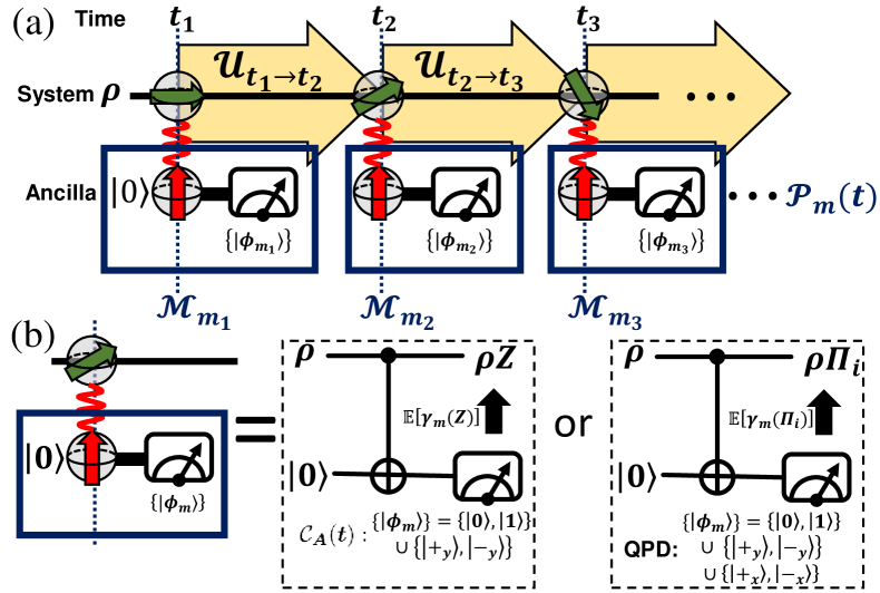
Figure 1: (a) Diagram for sequential ancilla-assisted measurements. (b) By adding more measurement bases on top of $\{\left|0\right>,\left|1\right>\}$ measurements, the quantum correlation function and the QPDs can be reconstructed from the ancilla measurement outcomes.

Our main goal is to extract quantum correlation function and QPDs without inducing measurement back-action. The main idea is finding a set of positive operator-valued measurements (POVMs) $\{M_{m}\}$ satisfying

$$\rho A=\sum_{m}\gamma_{m}(A)M_{m}\rho M_{m}^{\dagger},$$ (4)

with complex coefficients $\gamma_{m}(A)$. To meet the completeness relation, we also impose the condition $\sum_{m}M^{\dagger}_{m}M_{m}=\mathbb{1}$. In principle, any POVM element $M_{m}$ can be realized by introducing an ancilla state interacting with the system followed by the measurement of the ancilla state, as described in Fig. 1(a). Our main observation is that the $N$-time correlation function can be obtained as

$${\cal C}_{\bm{A}}(\bm{t})=\mathbb{E}\left[\gamma_{\bm{m}}(\bm{A})\right]=\sum_{\bm{m}}{\cal P}_{\bm{m}}(\bm{t})\left[\prod_{n=1}^{N}\gamma_{m_{n}}(A^{(n)})\right],$$ (5)

as an ensemble average over sequential outcome trajectories $\bm{m}:=(m_{1},m_{2},\cdots,m_{N})$. The probability distribution of the outcome $\bm{m}$ can explicitly be expressed as

$${\cal P}_{\bm{m}}(\bm{t})$$ (6)

$$\quad:={\rm Tr}\left[{\cal M}_{m_{N}}\circ\cdots\circ{\cal U}_{t_{2}\rightarrow t_{3}}\circ{\cal M}_{m_{2}}\circ{\cal U}_{t_{1}\rightarrow t_{2}}\circ{\cal M}_{m_{1}}(\rho)\right],$$

where ${\cal U}_{t_{i}\rightarrow t_{j}}(\rho):=U_{t_{i}\rightarrow t_{j}}\rho U_{t_{i}\rightarrow t_{j}}^{\dagger}$ and ${\cal M}_{m_{n}}:=M_{m_{n}}\rho M_{m_{n}}^{\dagger}$. We note that ${\cal P}_{\bm{m}}(\bm{t})$ is an experimentally accessible non-negative probability distribution, while the quantum correlation function can be reconstructed by taking complex-valued weights to it. As the measurement $\{M_{m}\}$ and the weights $\gamma_{m}(A)$ at each time can be constructed independent of the system’s dynamics, one can obtain joint distribution of various quantum dynamics without changing the measurement setting. Following the same argument, the QPDs can also be obtained from the sequential POVM outcomes as

$${\cal Q}_{\bm{i}}(\bm{t})=\mathbb{E}\left[\gamma_{\bm{m}}(\bm{\Pi}_{\bm{i}})\right],$$ (7)

where $\gamma_{\bm{m}}(\bm{\Pi}_{\bm{i}}):=\prod_{n=1}^{N}\gamma_{m_{n}}\left(\Pi^{(n)}_{i_{n}}\right)$.

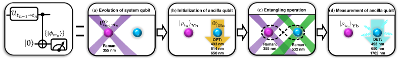
Figure 2: Ancilla-assisted sequential measurement realized in a ${}^{171}\rm{Yb}^{+}$-${}^{138}\rm{Ba}^{+}$ trapped-ion system. The ancilla-assisted measurement is performed as follows: (a) The system qubit involves the evolution ${\cal U}_{t_{n-1}\rightarrow t_{n}}$, then (b) initialize the ${}^{138}\rm{Ba}^{+}$ qubit to $\left|0\right>$ by optical pumping (OPT). (c) Perform a CNOT gate between two qubits through entangling operation. (d) Measure the ancilla qubit with fluorescence detection (DET). The whole round of measurement (b)–(d) is then completed.

While the proposed protocol extracts quantum statistics without measurement back-action, we highlight that it does not violate the information gain–disturbance trade-off relation Groenewold (1971); Fuchs and Peres (1996); Ozawa (2003); Buscemi et al. (2014); Fan et al. (2015); Lee et al. (2021); Hong et al. (2022). This can be observed from the fact that obtaining quantum statistics in Eqs. (5) and (7) requires more resources than classical statistics, as a larger number of trajectories should be collected to compensate the information disturbance caused by ancilla-assisted measurements. More precisely, the expectation value $\mathbb{E}\left[\gamma_{\bm{m}}(\bm{A})\right]$ fluctuates with $|\gamma|_{\rm max}:=\prod_{n=1}^{N}\left[\max_{m_{n}}\{|\gamma_{m_{n}}(A^{(n)})|\}\right]$ so that the number of trajectory for a desired precision scales with $|\gamma|^{2}_{\rm max}$ from Hoeffding’s inequality Hoeffding (1963).

We also note that our approach is free from the restrictions of the conventional approaches, which require either preparation of multiple copies of quantum states Perarnau-Llobet et al. (2017); Wu et al. (2019) or maintaining long time entanglement between the system and the ancilla Somma et al. (2002); Souza et al. (2011); Pedernales et al. (2014); Xin et al. (2017).

Explicit protocol for a two-level system.— For an given observable $A$, various choices of $\{M_{m},\gamma_{m}\}$ can be taken to satisfy Eq. (4). In order to focus on the statistics of a two-level system, we consider a POVM of the following form:

$$M_{m}=\frac{\langle\phi_{m}|0\rangle}{\sqrt{\alpha}}\left|0\right>\langle 0|+\frac{\langle\phi_{m}|1\rangle}{\sqrt{\alpha}}\left|1\right>\langle 1|,$$ (8)

where $\sum_{m}\left|\phi_{m}\right>\langle\phi_{m}|=\alpha\mathbb{1}$ and $\left|\phi_{m}\right>$ are not necessarily orthogonal to each other. Such a POVM can be implemented using ancilla-assisted measurement as follows: (i) prepare an ancilla state at $\left|0\right>$, (ii) interact the system and the ancilla via the CNOT-gate, (iii) measure the ancilla onto states $\left|\phi_{m}\right>$ (see Fig. 1). After the measurement, the ancilla qubit is re-initialized to $\left|0\right>$ so that it can be used for the measurement at the next time. We note that this scheme readily incorporates the classical projection measurements by performing the $z$-basis measurement of the ancilla state, i.e., $\{\left|\phi_{m}\right>\}=\{\left|0\right>,\left|1\right>\}$.

Quantum statistics can be obtained by taking more measurements on top of the $z$-basis measurement. For example, the Pauli-$Z$ operator, $Z=\left|0\right>\langle 0|-\left|1\right>\langle 1|$, acting on the right side of the quantum state, i.e., $\rho Z$ can be realized by a set of measurements $\{\left|\phi_{m}\right>\}=\{\left|0\right>,\left|1\right>,\left|+_{y}\right>,\left|-_{y}\right>\}$, where $\left|\pm_{y}\right>=(\left|0\right>\pm i\left|1\right>)/\sqrt{2}$ (see Fig. 1(b)). In this case, the weight can be calculated as $\{\gamma_{m}(Z)\}=\{2,-2,2i,-2i\}$. On the other hand, such a measurement set is not enough to obtain QPDs described in Eq. (7). This can be intuitively understood by the fact that QPDs contain more information than correlation function as seen in Eq. (3). We find that by adding $x$-basis measurements onto $\left|\pm_{x}\right>=(\left|0\right>\pm\left|1\right>)/\sqrt{2}$, which compose a set of measurements $\{\left|\phi_{m}\right>\}=\{\left|0\right>,\left|1\right>,\left|+_{y}\right>,\left|-_{y}\right>,\left|+_{x}\right>,\left|-_{x}\right>\}$ (see Fig. 1(c)), is sufficient to obtain QPDs with various choices of $\gamma_{m}(\Pi_{0})$ and $\gamma_{m}(\Pi_{1})$ (see Supplemental Material Sup for details and further generalizations).

Experimental realization.— We demonstrate the proposed protocol with two different species of ${}^{171}\rm{Yb}^{+}$ and ${}^{138}\rm{Ba}^{+}$ ions trapped in a single trap Wang et al. (2017, 2021, 2022). A crucial part of the protocol is repeated times of ancilla measurement and initialization without disturbing the system. The dual-species trapped-ion system provides a promising direction for this as each ion is controlled by lasers with different wavelengths. With minimal influence on each other, ICD and ICI on two different ions can independently performed Wang et al. (2022). In the experiment, two hyperfine levels in the $S_{1/2}$ of the ${}^{171}\rm{Yb}^{+}$ ion, $\left|F=0,m_{F}=0\right>\equiv\left|0\right>_{\mathrm{Yb}}$ and $\left|F=1,m_{F}=0\right>\equiv\left|1\right>_{\mathrm{Yb}}$ with the energy splitting of 12.6428 GHz, serves as the system qubit. The qubit is insensitive to environmental noise and demonstrated a long coherence time. For the ${}^{138}\rm{Ba}^{+}$ ion, two Zeeman levels in the $S_{1/2}$ manifold are encode as the ancilla qubit, $\left|s_{j}=1/2\right>\equiv\left|0\right>_{\mathrm{Ba}}$ and $\left|s_{j}=-1/2\right>\equiv\left|1\right>_{\mathrm{Ba}}$ with the energy splitting of 16.2 MHz. Raman transitions are used to manipulate the ${}^{171}\rm{Yb}^{+}$ and ${}^{138}\rm{Ba}^{+}$ qubits with 355 nm and 532 nm lasers, respectively, as shown in Fig. 2. For the entangling operations for ${}^{171}\rm{Yb}^{+}$ and ${}^{138}\rm{Ba}^{+}$ qubits, we simultaneously apply the 355 nm and 532 nm laser beams with properly chosen frequencies.

Figure 3: (a) Two- and (b) three-time correlation functions reconstructed from the ancilla-assisted measurements of the ${}^{171}\rm{Yb}^{+}$-${}^{138}\rm{Ba}^{+}$ system. The real (blue) and imaginary (red) parts of the correlation functions obtained in the experiments are represented in dots, while solid and dashed curves refer to imaginary and real parts of the theoretical values, respectively. (c) Two- and (d) three-time QPDs reconstructed from the outcome trajectories for $\theta=0.3\pi$ and $\theta=0.74\pi$, respectively. The horizontal index $\bm{i}=(i_{1},i_{2},\cdots)$ indicates the projection operator $\Pi_{i_{n}}$ at time $t_{n}$ described in Eq. (2). For the three-time QPDs, negativity is verified for (0,1,0) and (1,1,0), pointed in red-dashed-line boxes. (e) The marginal distributions of the $z$-basis measurement at time $t_{2}$. Dots are reconstructed from the experimental data where three-time ancilla-assisted measurements are performed. Solid and dashed lines refer to the exact $z-$population when no measurement is performed before $t_{2}$. dash-dotted line refers to the $z-$population when projection measurements are performed at time $t_{1}$ or $t_{2}$, which is balanced for every $\theta$. (f) Leggett-Garg inequality test with three-time QPDs (blue) and projection measurements (gray). Dots are experimental data. Solid curves are theoretical prediction. At the point $\theta=0.74\pi$ from three-time QPDs, we obtain $K\approx 1.17$, which violates the classical bound $1$. For all the data, the dynamics are given as $U_{t_{1}\rightarrow t_{2}}=R_{x}(\theta)$ and $U_{t_{2}\rightarrow t_{3}}=R_{y}(\theta^{2})$, and error bars represent the standard error of the mean (SEM). For each measurement configuration, $100$ outcome trajectories are collected.

We first prepare the system qubit to $\left|+\right>_{\mathrm{Yb}}=\frac{1}{\sqrt{2}}(\left|0\right>_{\mathrm{Yb}}+\left|1\right>_{\mathrm{Yb}})$ and the ancilla qubit to $\left|0\right>_{\mathrm{Ba}}$ (at $t_{1}$ in Fig. 1(a)). The initialization to $\left|0\right>_{\mathrm{Yb(Ba)}}$ states is performed by the standard optical pumping methods for both ${}^{171}\rm{Yb}^{+}$ and ${}^{138}\rm{Ba}^{+}$ ions Wang et al. (2022). We then use 355 nm laser beams to prepare $\left|+\right>_{\mathrm{Yb}}$ state. The system state then evolves under a single-qubit $x$-axis rotation $U_{t_{1}\rightarrow t_{2}}=R_{x}(\theta)=R(\theta,0)$ (from $t_{1}$ to $t_{2}$) followed by $y$-axis rotation $U_{t_{2}\rightarrow t_{3}}=R_{y}(\theta^{2})=R(\theta^{2},-\pi/2)$ with $\theta\in[0,\pi]$ (from $t_{2}$ to $t_{3}$), both of which are performed by applying 355 nm laser beams. Here a general single-qubit rotation is defined as $R(\theta,\phi)=\left(\begin{array}[]{cc}\cos(\frac{\theta}{2})&-ie^{-i\phi}\sin(\frac{\theta}{2})\\ -ie^{i\phi}\sin(\frac{\theta}{2})&\cos(\frac{\theta}{2})\end{array}\right)$. At each time, the ancilla-assisted measurement is realized by the CNOT gate between the system (${}^{171}\rm{Yb}^{+}$) and ancilla (${}^{138}\rm{Ba}^{+}$) states followed by the projection measurement of the ancilla. The Mølmer-Sørensen (M-S) gate Sørensen and Mølmer (1999) is used to construct the CNOT gate. The average fidelity of the M-S gate is $94\pm 2\%$ in the experiment. Details of the M-S gate and its imperfection are described in Supplemental Material Sup .

The measurement of the ${}^{138}\rm{Ba}^{+}$ ion is realized by applying detection laser after shelving $\left|0\right>_{\mathrm{Ba}}$ state to $D_{5/2}$ manifold with the help of 1762 nm narrow linewidth laser, where detection fidelity is $98.9\%$. In order to simplify the experimental steps, the final measurement is replaced by the projection measurement on the ${}^{171}\rm{Yb}^{+}$ ion as we do not need to worry about the system disturbance. The detection fidelity of ${}^{171}\rm{Yb}^{+}$ ion is $98.4\%$. The detection infidelities are improved by using the detection-error correct method introduced in Ref. Shen and Duan (2012) for both ${}^{171}\rm{Yb}^{+}$ and ${}^{138}\rm{Ba}^{+}$ ions.

We reconstruct correlation functions from the experimental measurement results. Fig. 3(a) and (b) show the two- and three-time correlation functions ${\cal C}_{ZZ}(t_{1},t_{2})$ and ${\cal C}_{ZZZ}(t_{1},t_{2},t_{3})$ reconstructed from the experimental measurements. The two-time correlation function is in a good agreement with the theoretical predictions, while the three-time correlation function has relatively large deviations. This is mainly because of that adding more measurement steps induces a larger fluctuation of $\gamma_{\bm{m}}=\prod_{n=1}^{N}\gamma_{m_{n}}$ for each realization. Another reason is that durations for the ancilla measurements are relatively long to collect enough fluorescence, which introduces large phase fluctuations and degrades the performance of the CNOT gates.

Fig. 3(c) and (d) show the two- and three-time QPDs ${\cal Q}_{\bm{i}}(t_{1},t_{2})$ and ${\cal Q}_{\bm{i}}(t_{1},t_{2},t_{3})$ obtained by collecting additional trajectories including the $x$-basis measurement at $t_{1}$ and $t_{2}$. To our knowledge, it is the first experimental reconstruction of the QPDs beyond two-time points. The negativity in real parts as well as non-vanishing imaginary parts are clearly observed in the experimentally reconstructed three-time QPDs (see Fig. 3(d)). The contribution of coherence can be clearly seen by comparing the marginal distribution at time $t_{3}$ of the reconstructed QPDs with the projection measurement case. When the projective measurement is performed to the initial state $\rho=\left|+\right>\langle+|$, the state after the measurement becomes the maximally mixed state without any coherence, $\rho^{\prime}=\sum_{i}\Pi_{i}\rho\Pi_{i}=\mathbb{1}/2$, so that the population is always balanced at $t_{3}$ regardless of the unitary dynamics $U_{t_{1}\rightarrow t_{2}}$ and $U_{t_{2}\rightarrow t_{3}}$. Fig. 3(e) shows that the marginal distribution at $t_{3}$ is not always balanced but varies by taking different unitary dynamics, following the quantum mechanical prediction without measurement back-action.

While the negative and non-real values can already be interpreted as a nonclassical feature of QPDs, a stronger notion of nonclassicality can be witnessed by Leggett-Garg inequality violation Leggett and Garg (1985). For any classical joint probability distribution $P(i_{1},i_{2},i_{3})$ and a bounded function $E_{t_{n}}(i_{n})\in\{1,-1\}$ at each time $t_{n}$, the following inequality should hold:

$$K=\langle E_{t_{1}}E_{t_{2}}\rangle+\langle E_{t_{2}}E_{t_{3}}\rangle-\langle E_{t_{1}}E_{t_{3}}\rangle\leq 1,$$ (9)

which was introduced by Leggett and Garg Leggett and Garg (1985) to test microscopic realism. By taking $E_{t_{1}}(i_{1})=(-1)^{i_{1}}$, $E_{t_{2}}(i_{2})=1$, and $E_{t_{3}}(i_{3})=(-1)^{i_{3}}$, we observe the violation of Eq. (9) with $K\approx 1.17$ from the real part of the experimentally reconstructed three-time QPDs (see Fig. 3(f)). This strongly supports that the reconstructed QPDs can be sharply distinguished from classical distributions.

Remarks.— We have proposed and experimentally demonstrated a measurement scheme to overcome the measurement back-action in obtaining multi-time quantum statistics. Using the ${}^{171}\rm{Yb}^{+}$-${}^{138}\rm{Ba}^{+}$ trapped-ion system, we have experimentally demonstrated that two- and three-time quantum correlation functions and QPDs reconstructed from the ancilla-assisted measurements follow the quantum mechanical prediction with full contributions of coherence.

We highlight that our method is not limited to the two-level system and can be generalized to any $d$-dimensional quantum system by replacing the CNOT gate with the CSUM gate, $U_{\rm CSUM}=\sum_{i,j=0}^{d-1}\left|i,i\oplus j\right>\langle i,j|$ and taking informationally complete basis measurements on a $d$-dimensional ancilla state Sup . Furthermore, it is straightforward to extend the protocol to be applied to non-unitary dynamics, by simply replacing ${\cal U}_{t_{i}\rightarrow t_{j}}$ in Eq. (6) to any completely positive trace-preserving quantum channel. As the ancilla-assisted measurement protocol is independent of the system’s dynamics and only requires a single copy of the system state with a short time system-ancilla interaction, our approach can be a useful experimental tool for exploring quantum statistics of both open and closed quantum systems.

Note added.– While preparing the manuscript, we recognized a recent work Del Re et al. (2022) which deals with the multi-time correlation function.

Supplemental Material for “Demonstration of multi-time quantum statistics without measurement back-action”

I Experimental Methods

I.1 Experimental circuit

Multi-time measurement circuit is shown in Fig. 4(a). The system qubit information is measured with the assistance of ancilla qubit. The ancilla qubit is connected to the system qubit via a CNOT gate consisting of a Mølmer-Sørensen (M-S) gate and four single qubit rotations, as shown in Fig. 4(b). Before applying the M-S gate, the average phonon number in the axial out-of-phase (in-phase) mode is cooled to 0.04 (0.11) by three steps: Doppler cooling, electromagnetically-induced-transparency (EIT) cooling, and Raman sideband cooling. State fidelity of the Bell state created by the M-S gates is $0.94\pm 0.02$, which is limited by parameter shift in long-sequence operations and the axial in-phase mode cooling imperfection.

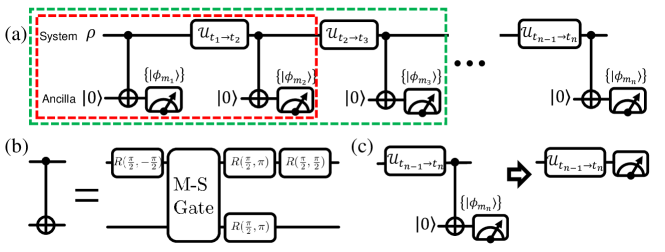
Figure 4: Experimental circuit for multi-time measurement. (a) The system and ancilla qubits are first prepared to $\rho$ and $\left|0\right>$, respectively. The first-time measurement starts with a CNOT gate between the system and the ancilla, followed by a measurement of the ancilla qubit. After a unitary evolution ${\cal U}_{t_{1}\rightarrow t_{2}}$ on the system qubit, a second-time measurement is performed with a similarly process to the first one. This scheme can be directly extended to multi-time measurement. Red and green boxes indicate the two-time and three-time measurement, respectively. (b) The CNOT gate is composed of a M-S gate and four-single qubit rotations. The M-S gate can be described as $\exp(i\frac{\pi}{4}X\otimes X)$, where $X$ is the Pauli operator. The single-qubit rotation is defined as $R(\theta,\phi)=\left(\begin{array}[]{cc}\cos(\frac{\theta}{2})&-ie^{-i\phi}\sin(\frac{\theta}{2})\\ -ie^{i\phi}\sin(\frac{\theta}{2})&\cos(\frac{\theta}{2})\end{array}\right)$. (c) The last-time measurement can be performed by direct measurement in basis $m_{2}\in\{\left|0\right>_{z},\left|1\right>_{z}\}$ on the system qubit since coherence is no more needed for further measurement.

I.2 Experimental setup for ancilla-assisted measurement

As shown in Fig. 5(a), a dual-species trapped-ion system, which traps one ${}^{171}\rm{Yb}^{+}$ ion and one ${}^{138}\rm{Ba}^{+}$ ion in a four-rod trap, is used to realize the ancilla-assisted measurements. ${}^{171}\rm{Yb}^{+}$ and ${}^{138}\rm{Ba}^{+}$ ions serve as the system and the ancilla respectively. The two ions have different energy structures, and require different initialization and detection lasers. Therefore, the operation on one ion does not affect the other ion. It is thus possible to perform in-circuit detection (ICD) and initialization (ICI), where one qubit is detected or initialized without affecting the other qubit.Wang et al. (2022). This special property is essential for the ancilla-assisted measurement. Experimentally, we also need single-qubit rotations and two-qubit M-S gate. As shown in Fig. 5, we use 355 nm and 532 nm Raman transitions to realize gate operations of ${}^{171}\rm{Yb}^{+}$ and ${}^{138}\rm{Ba}^{+}$ ions, respectively.

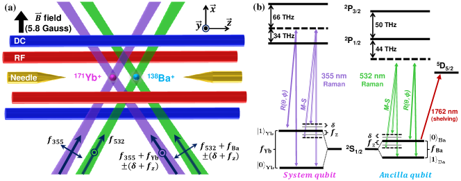
Figure 5: Experimental setup. (a) ${}^{171}\rm{Yb}^{+}$ and ${}^{138}\rm{Ba}^{+}$ ions trapped in a four-rod trap. The magnetic field of 5.8 Gauss is applied along the $x$-axis. In order to realize M-S gate between two ions, the ${}^{171}\rm{Yb}^{+}$ ion is controlled by illuminating a pair of 355 nm lasers (purple) with a frequency of $f_{355}$ and $f_{355}+f_{\mathrm{Yb}}\pm(\delta+f_{z})$, where $f_{\mathrm{Yb}}$ is the qubit splitting of ${}^{171}\rm{Yb}^{+}$ qubit. The ${}^{138}\rm{Ba}^{+}$ ion is controlled by illuminating a pair of 532 nm lasers (green) with a frequency of $f_{532}$ and $f_{532}+f_{\mathrm{Ba}}\pm(\delta+f_{z})$, where $f_{\mathrm{Ba}}$ is the qubit splitting of ${}^{138}\rm{Ba}^{+}$ qubit, $f_{z}$ is the axial OOP (out-of-phase) mode frequency, and $\delta$ is the laser detuning from the sideband of OOP mode. Raman laser directions are represented by thick arrows, and polarization is represented by thin arrows and dots. (b) Energy level and related lasers for ${}^{171}\rm{Yb}^{+}$ and ${}^{138}\rm{Ba}^{+}$ ions. The ${}^{171}\rm{Yb}^{+}$ ion’s hyperfine qubit and ${}^{138}\rm{Ba}^{+}$ ion’s Zeeman qubit serve as the system qubit and the ancilla qubit, respectively. Single-qubit rotations are realized by resonant Raman transitions. Two-qubit entangling operation is realized by applying bichromatic Raman laser for both ions. The 1762 nm laser is the shelving laser used for ${}^{138}\rm{Ba}^{+}$ qubit detection.

I.3 Post-selection detection

Fig. 6 shows the detailed process of the ${}^{138}\rm{Ba}^{+}$ ion fluorescence detection. In this detection process, we first use 1762 nm laser to shelve $\left|0\right>_{\mathrm{Ba}}$ population to $\mathrm{D}_{5/2}$, and then apply 493 nm laser to drive the transition between $\mathrm{S}_{1/2}$ and $\mathrm{P}_{1/2}$. If the qubit state is $\left|1\right>_{\mathrm{Ba}}$, the shelving operation has no effect and the later 493 nm laser will produce a large number of photons. But if the qubit state is $\left|0\right>_{\mathrm{Ba}}$, the population is shelved to $\mathrm{D}_{5/2}$ and the 493 nm laser does not produce any photons. Then qubit states can be distinguished by the number of photons scattered.

In our multi-time measurements circuit, the ancilla (${}^{138}\rm{Ba}^{+}$ ) needs to be repeatedly detected and used. However, as shown in Fig. 6(a), the detecting of bright state produces a large number of photons, thereby heats the ion chain and further degrades the performance of subsequent CNOT operations. To solve this problem, we adopt a post-selection approach for all ICD, which use only dark state data. For bright state data, we transfer the bright state to dark state by $\pi$ flip pulse and then measure.

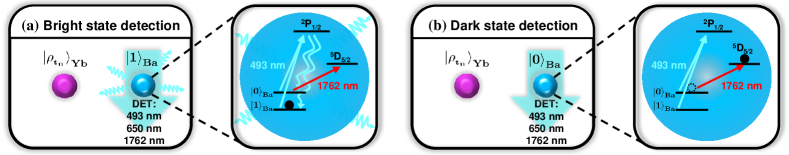
Figure 6: Fluorescence detection of ${}^{138}\rm{Ba}^{+}$ ion. The detection process involves two steps: first, use a 1762 nm laser to shelve the $\left|0\right>_{\mathrm{Ba}}$ population to $\mathrm{D}_{5/2}$, and then use a 493 nm laser to drive the transition between $\mathrm{S}_{1/2}$ and $\mathrm{P}_{1/2}$. (a) Bright state detection. when the ancilla is at state $\left|1\right>_{\mathrm{Ba}}$, the shelving operation has no effect on the qubit. The later 493 nm laser produces a large number of photons. (b) Dark state detection. When the ancilla is at state $\left|0\right>_{\mathrm{Ba}}$, its population will be shelved to $\mathrm{D}_{5/2}$. Therefore, the 493 nm laser does not produce any photons.

II Obtaining quantum statistics from POVM measurements

II.1 General conditions

For a $d$-dimensional quantum system. Let us consider a slightly more general scenario such that operators are acting both on left and right-side of the density matrix:

$$B\rho A=\sum_{m}\gamma_{m}(B,A)M_{m}\rho M_{m}^{\dagger},$$ (10)

where the case discussed in the main text is a special case by taking $B=I$. We also generalize the POVM measurements by introducing an ancilla state having the same dimension as the system, initially prepared at $\left|0\right>_{R}$. After applying the CSUM gate, a generalized CNOT gate, $U_{\rm CSUM}=\sum_{i,j=0}^{d-1}\left|i,i\oplus j\right>\langle i,j|$ followed by the ancilla measurement onto the states $\{\left|\phi_{m}\right>_{R}\}$ satisfying $\sum_{m}\left|\phi_{m}\right>\langle\phi_{m}|=\alpha\mathbb{1}$, we can construct each POVM element as,

$$M_{m}=\frac{\langle\phi_{m}|U_{\rm CSUM}\left|0\right>_{R}}{\sqrt{\alpha}}=\sum_{i=0}^{d-1}\left(\frac{\langle\phi_{m}|i\rangle_{R}}{\sqrt{\alpha}}\right)\left|i\right>\langle i|.$$ (11)

We then find a sufficient condition for a set of measurements $\{\left|\phi_{m}\right>\}$ to reconstruct the operation in Eq. (10) for diagonal operators $A$ and $B$ as follows:

Proposition 1 (Sufficient condition of a measurement set).

For operators $A=\sum_{i}a_{i}\left|i\right>\langle i|$ and $B=\sum_{i}b_{i}\left|i\right>\langle i|$ that are diagonal in the basis $\left|i\right>$, there always exists $\gamma_{m}(B,A)$ satisfying Eq. (10) for a measurement set $\{\left|\phi_{m}\right>\}$ which is informationally complete.

Proof.

By definition of a set of informationally complete states, one can express any operator $O$ (no matter Hermitian or not) as $O=\sum_{m}c_{m}(O)\left|\phi_{m}\right>\langle\phi_{m}|$ with some complex coefficients $c_{m}(O)$. Now let’s take an operator $O(B,A)$ as follows:

$$O(B,A)=\sum_{i,j=0}^{d-1}a_{i}b_{j}\left|i\right>\langle j|=\sum_{m}c_{m}(O(B,A))\left|\phi_{m}\right>\langle\phi_{m}|.$$ (12)

We then observe that taking $\gamma_{m}(B,A)=\alpha c_{m}(O(B,A))$ leads to

$$\sum_{m}\gamma_{m}(B,A)M_{m}\rho M_{m}^{\dagger}$$ (13)

$$=\sum_{m}\sum_{i,j=0}^{d-1}c_{m}(O(B,A))\langle i|\phi_{m}\rangle\langle\phi_{m}|j\rangle\left|j\right>\langle j|\rho\left|i\right>\langle i|$$

$$=\sum_{i,j=0}^{d-1}a_{i}b_{j}\left|j\right>\langle j|\rho\left|i\right>\langle i|$$

$$=B\rho A,$$

which completes the proof. ∎

As an informationally complete basis has at least $d^{2}$ elements for a $d$-dimensional system, we note that obtaining the quantum statistics in the form of Eq. (10) always requires more measurement setting than the projection measurements $\{\Pi_{i}\}_{i=0}^{d-1}$. However, there could be an informationally incomplete measurement set even with $d^{2}$ elements. For example, for the measurement sets discussed in the main text, $\{\left|\phi_{m}\right>\}=\{\left|0\right>,\left|1\right>,\left|+_{y}\right>,\left|-_{y}\right>\}$ is not informationally complete, while $\{\left|\phi_{m}\right>\}=\{\left|0\right>,\left|1\right>,\left|+_{y}\right>,\left|-_{y}\right>,\left|+_{x}\right>,\left|-_{x}\right>\}$ is informationally complete. Nevertheless, such the measurement set based on the Pauli basis is easier to be realized in experiments.

II.2 Optimizing the weights

When a set of POVM $\{M_{m}\}$ to obtain the statistics of hermitian operators $A$ and $B$ is overcomplete, there could be a various choice of weight vector $\gamma_{m}(B,A)$ satisfying Eq. (10). As the expectation value $\mathbb{E}\left[\gamma_{m}(B,A)\right]$ fluctuates with $|\gamma(B,A)|_{\rm max}:=\max_{m}\{|\gamma_{m}(B,A)|\}$, the optimal choice would be to minimize $|\gamma|_{\rm max}$. Such a optimization problem can be expressed as:

$${\rm for~{}given:} \qquad A,~{}B,~{}\{M_{m}\}$$ (14)

$${\rm minimize:} \qquad|\gamma|_{\rm max}=\max_{m}\{|\gamma_{m}|\}$$ (15)

$${\rm subject~{}to:} \qquad B\otimes A^{T}=\sum_{m}\gamma_{m}M_{m}\otimes M_{m}^{*}.$$ (16)

For $A$ and $B$ that are diagonal in the same basis $\{\left|i\right>\}$ and the POVM measurement described in Eq. (11), the condition in Eq. (16) reduces to

$$\bm{T}\bm{\gamma}=\alpha\bm{y},$$ (17)

where $[\bm{T}]_{i+jd,m}=\langle\phi_{m}|j\rangle\langle i|\phi_{m}\rangle$, $[\bm{\gamma}]_{m}=\gamma_{m}$, and $[\bm{y}]_{i+jd}=a_{i}b_{j}$. For the correlation function discussed in the main text, the weight vector $\{\gamma_{m}(I,Z)\}=\{2,-2,2i,-2i\}$ with the measeurement set $\{\left|\phi_{m}\right>\}=\{\left|0\right>,\left|1\right>,\left|+_{y}\right>,\left|-_{y}\right>,\left|+_{x}\right>,\left|-_{x}\right>\}$ yields the minimum value of $|\gamma(I,Z)|_{\rm max}=2$. For the QPD reconstruction, the numerical optimization for the measurement set $\{\left|\phi_{m}\right>\}=\{\left|0\right>,\left|1\right>,\left|+_{y}\right>,\left|-_{y}\right>,\left|+_{x}\right>,\left|-_{x}\right>\}$ leads to $|\gamma(I,\Pi_{i})|_{\rm max}\approx 1.775$.