Automated Detection of Label Errors in Semantic Segmentation Datasets via Deep Learning and Uncertainty Quantification

Abstract

In this work, we for the first time present a method for detecting label errors in image datasets with semantic segmentation, i.e., pixel-wise class labels. Annotation acquisition for semantic segmentation datasets is time-consuming and requires plenty of human labor. In particular, review processes are time consuming and label errors can easily be overlooked by humans. The consequences are biased benchmarks and in extreme cases also performance degradation of deep neural networks (DNNs) trained on such datasets. DNNs for semantic segmentation yield pixel-wise predictions, which makes detection of label errors via uncertainty quantification a complex task. Uncertainty is particularly pronounced at the transitions between connected components of the prediction. By lifting the consideration of uncertainty to the level of predicted components, we enable the usage of DNNs together with component-level uncertainty quantification for the detection of label errors. We present a principled approach to benchmarking the task of label error detection by dropping labels from the Cityscapes dataset as well from a dataset extracted from the CARLA driving simulator, where in the latter case we have the labels under control. Our experiments show that our approach is able to detect the vast majority of label errors while controlling the number of false label error detections. Furthermore, we apply our method to semantic segmentation datasets frequently used by the computer vision community and present a collection of label errors along with sample statistics.

1 Introduction

In many applications such as automated driving and medical imaging, large amounts of data are collected and labeled with the long-term goal of obtaining a strong predictor for such labels via artificial intelligence, in particular via deep learning [24, 13, 19, 25, 29, 21]. Acquisition of so-called semantic segmentation ground truth, i.e., the pixel-wise annotation within a chosen set of classes on which we focus in this work, involves huge amounts of human labor. A German study states an effort of about 1.5 working hours per high definition street scene image [33]. Typically, industrial and scientific labelling processes consist of an iterative cycle of data labeling and quality assessment. Since the long-term goal of acquiring enough data to train e.g. deep neural networks (DNNs) to close to ground truth performance requires huge amounts of data, partial automation of the labeling cycle is desirable. Two research directions aiming at this goal are active learning, which aims at labeling only those data points that leverage the model performance a lot (see e.g. [22, 6, 34]), and the automated detection of label errors (see [28, 9]). Currently, in active learning for semantic segmentation, a moderate number of methods exists. This is also due to the fact that active learning comes with an increased computational cost as a DNN has to be trained several times over the course of the active learning iterations [22, 6]. Typically, these methods assume that perfect ground truth can be obtained by an oracle/teacher in each active learning iteration. In practice this is not the case and annotations are subject to multiple review loops. In that regard, current methods mostly study how noisy labels affect the model performance [16, 44], with the insight that DNNs can deal with a certain amount of label noise quite well. Methods for modeling label uncertainty in medical image segmentation, semantic street scene segmentation and everyday scene segmentation were proposed in [23, 38, 18, 45, 42].

For image classification tasks, the detection of label errors was studied in [28]. Importantly, it was pointed out that label errors harm the stability of machine learning benchmarks [27]. This stresses the importance of being able to detect label errors, which will help to improve model benchmarks and speed up dataset review processes.

In this work, we for the first time study the task of detecting label errors in semantic segmentation in settings of low inter- and intra-observer variability. While DNNs provide predictions on pixel level, we assess DNN predictions on the level of connected components belonging to a given class by utilizing [31]. Note that this is crucial since a connected component has uncertain labels at its boundary, which makes label error detection on pixel level a complex task. For each connected component, we estimate the probability of that prediction being correct. If a connected component has a high estimated probability of being correct, while it is signaled to be false positive w.r.t. ground truth, we consider that component as a potential label error. We study the performance of our label error detection method on synthetic image data from the driving simulator CARLA [10] and on Cityscapes [8]. CARLA gives us a guarantee of being per se free of label errors such that we can provide a clean evaluation. To this end, we remove objects from the ground truth and study whether our method is able to identify these components as overlooked by the ground truth. Cityscapes provides high quality ground truth with only a small amount of label errors. The ground truth is available in terms of polygons such that we can drop connected components as well. In both cases it turns out that our method is able to detect most of the dropped labels while keeping the amount of false positive label errors under control. We believe that our method offers huge potential to make labeling processes more efficient. Our contribution can be summarized as follows:

• We for the first time present a method that detects label errors in semantic segmentation.

• Utilizing [31] we detect label errors on the level of connected components.

• We introduce a principled benchmark for the detection of label errors based on [10] and [8].

• We apply our method to additional datasets [1, 12, 47] and provide examples of label errors that we found. By manually assessing samples of that data we evaluate the precision of our method on those datasets.

For all of those four real-world datasets we studied, we achieved a precision between $47.5\%$ and $67.5\%$ of correctly predicted label errors. We show that our method is able to find both overlooked and class-wise flipped labels while keeping the amount of prediction to review considerably low.

2 Related Work

Figure 1: A visualization of our method for label error detection.

The impact of label errors on DNNs is an active field of research. Dataset labels in the context of classification have been shown to be imperfect [27], which also holds true for semantic segmentation. Particularly in medical images, regions of interest are often difficult to find due to visual ambiguity and inter- and intra-observer variability. For CT scans, the authors of [16] observed model performance degradation when the label error noise increases. Hence, a number of works focus on modelling label uncertainty and develop more robust segmentation models [23, 38, 18, 45, 42]. Up to now, to the best of our knowledge the detection of incorrectly labeled ground truth connected components in semantic segmentation has not been tackled. Major challenges are the inter- and intra-observer variability in applications like medical imaging, but also the fact that segmentation networks operate on pixel level.

In the context of image classification, learning methods that are robust to label noise have been introduced in [28, 17, 41, 39, 43, 20, 15, 14, 30], and also the problem of label error detection has been considered in [28]. The authors of [28] model class-conditional but image/instance-independent label noise in order to model label uncertainty and consider the task of label error detection. Indeed, the authors find numerous label errors in typical benchmark datasets like MNIST (image classification) or Amazon Reviews (sentiment classification). In [27], it is also pointed out that label errors in test sets destabilize prominent machine learning benchmarks such as MNIST, CIFAR10, CIFAR100, ImageNet, IMDB and Amazon Reviews. Another work [5] uses a cross validation approach that turns out to filter samples with noisy labels. However, for this filtering technique only the overall label quality is considered as a benchmark. In that work, label errors are not detected on an image level.

Our work for the first time tackles the task of label error detection in semantic segmentation, introducing a principled benchmark for the given task. An advanced post-processing method for DNN predictions lifts the problem of label error detection to the level of connected components and on that level yields calibrated estimate of the probability that a predicted connected component is indeed a correct prediction.

3 Label Error Detection Method

Estimating the probability of a prediction being correct.

We denote a given image by $x\in[0,1]^{n}$ with a label $y\in\{0,\ldots,c\}^{n}$ being a ground truth segmentation mask over $c$ classes created by human labor. We assume to have access to a trained neural network $f$ that provides for each image pixel $z$ an estimated probability distribution $f_{z}(y|x)$ over the $c$ classes. Given an image $x$, let $\hat{y}=\mathrm{arg\,max}_{i}f_{\cdot}(i|x)$ denote the predicted segmentation mask and $\hat{K}=\hat{K}(x)$ the set of connected components of $\hat{y}$. Analogously, let $K=K(x)$ denote the set of connected components in the ground truth $y$. For two pixels $z,z^{\prime}$ of the same predicted class, if $z^{\prime}$ is in the 8-pixel neighborhood of $z$, then they both belong to the same predicted connected component $\hat{k}\in\hat{K}$. We proceed analogously for $k\in K$.

Similarly to what is best practice in object detection, we call a connected component of the ground truth a true positive if it overlaps with a predicted connected component of the same class to a chosen degree. To this end, we use an adjusted version of the intersection over union ($\mathrm{IoU}$) from [2, 31] which is a map $\mathrm{sIoU}:K\to[0,1]$. For $k\in K$, it is defined as

$$\begin{split}&\mathrm{sIoU}(k):=\frac{|k\cap\mathit{pr}(k)|}{|(k\cup\mathit{pr}(k))\setminus A(\hat{k})|},\\ \text{ with}\qquad&\mathit{pr}(k)=\!\!\!\!\!\!\bigcup_{\hat{k}\in\hat{K},\hat{k}\cap k\neq\emptyset}\!\!\!\hat{k}~{}~{}~{}\end{split}$$ (1)

and $A(k)=\{z\in k^{\prime}:k^{\prime}\in K\setminus\{k\}\}$. The adjustment $A(k)$ excludes pixels from the union that are contained in another ground truth component $k^{\prime}\in K$ of the same class, which, however, is not equal to $k$. This can happen when a predicted component intersects with multiple ground truth components. That case is punished less by the $\mathrm{sIoU}$ than by the ordinary $\mathrm{IoU}$, we refer to [2, 31] for further details.

Given a threshold $\tau\in[0,1)$, we call a ground truth component $k\in K$ true positive ($\mathrm{TP}_{o}$ where $o$ refers to the “original” task of the DNN) if $\mathrm{sIoU}(k)>\tau$, and false negative ($\mathrm{FN}_{o}$) otherwise.

For the remaining error, i.e., a false positive ($\mathrm{FP}_{o}$) connected component $\hat{k}\in\hat{K}$ of the prediction, we compute a quantity similar to the precision:

$$\pi(\hat{k}):=\frac{|\hat{k}\cap g(\hat{k})|}{|\hat{k}|}~{}~{}~{}~{}~{}\text{ with }~{}~{}~{}~{}\mathit{g}(\hat{k})=\!\!\!\!\!\!\bigcup_{k\in K,\hat{k}\cap k\neq\emptyset}\!\!\!k\,.~{}~{}~{}$$ (2)

We call a predicted component $\hat{k}\in\hat{K}$ $\mathrm{FP}_{o}$ if $\pi(\hat{k})\leq\tau$.

We utilize a so-called meta classifier that was introduced in [31] and further extended in [32, 26, 3]. It was shown empirically in [7] that meta classification yields calibrated confidences on component level. Such a meta classifier computes a fixed number of $n_{f}$ hand-crafted features for each predicted component $\hat{k}\in\hat{K}$ yielding a structured dataset $\mathcal{M}$ of $n_{f}$ columns and $n_{\mathit{comp}}=\sum_{x}|\hat{K}(x)|$ rows, where $n_{\mathit{comp}}$ is the number of predicted components in a given number of images where the latter were not seen by the network $f$ during training (e.g. from a validation set). The hand-crafted features include metrics quantifying morphological features of the connected components as well as softmax uncertainty measures aggregated (average pooled) over the predicted components. For details we refer to the cited works. The meta classifier then performs a classification of $\mathrm{TP}_{o}$ vs. $\mathrm{FP}_{o}$ by means of the hand-crafted features. We utilize this meta classifier $m:\mathcal{M}\to[0,1]$ that yields an estimated probability for $\hat{k}$ being $\mathrm{TP}_{o}$, i.e., an estimate $m(\hat{k})\approx P(\mathrm{TP}_{o})$. Due to the estimate $m(\hat{k})$ being calibrated, we can expect that it is reflective of the model’s accuracy, i.e., when considering estimated probabilities in a chosen range, say 90%–95%, one can expect the accuracy to be in the same range.

Detection of label errors.

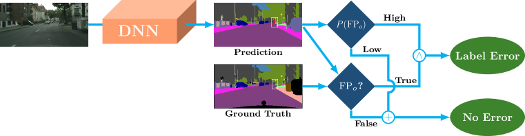
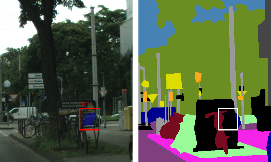
Our label error detection method is visualized in fig. 1. It utilizes a state-of-the-art semantic segmentation DNN that is trained on a given training set. Then, we consider any sample of data not seen during training and want to detect label errors. To this end, we infer predictions from the DNN and then compare the predicted components with the ground truth components. If a component $\hat{k}$ is $\mathrm{FP}_{o}$, this can mean that 1) the network is indeed producing a false positive and the ground truth is likely to be correct, or 2) the ground truth is incorrect and the DNN could be correct. At this point we consider the estimate $m(\hat{k})\approx P(\mathrm{TP}_{o})$. If our calibrated meta classifier yields a estimate $m(\hat{k})$ close to $1$, the network’s prediction is likely to be correct. Hence, any predicted component $\hat{k}$ being $\mathrm{FP}_{o}$ but having high $m(\hat{k})\approx P(\mathrm{TP}_{o})$ is considered as a candidate for review as it probably has been overlooked (or its label has been flipped) during labeling. Otherwise, we consider the prediction as not being suspicious.

Note that, in principle $P(\mathrm{TP}_{o})$ can also be replaced by any uncertainty estimate that, however, must operate on the level of predicted components. On trend, the method will improve with stronger DNNs and stronger meta classifiers / uncertainty estimates, which also highlights the generic nature of our approach. As already mentioned, our approach is concerned with finding label errors in data that was not used during training. Though, our method can be easily applied to entire datasets by training in a $k$-fold cross-validation fashion.

4 Datasets and Benchmarks for Label Error Detection in Semantic Segmentation

In a best case scenario, an evaluation protocol for label error detection methods has access to a perfectly clean ground truth (which does not exist in practice) where there are no label errors included, and another perturbed ground truth where there are labels missing or incorrect. A proper definition of label error itself is already difficult and subject to uncertainty.

Definition of label error.

In this work, we consider a label error as a connected component of a given class that, given the context of the input image, should be contained in the ground truth, but is not contained therein.

It may happen that a spurious connected component is inserted into a ground truth, not corresponding to anything visible in the image. Such cases, however, are rare in the datasets we examined.

Benchmark definition.

In our benchmark we focus on label errors that occur due to miss-outs rather than by accidentally selecting a wrong class. Note that creating such a benchmark poses a more complex task than flipping class labels. Furthermore, this is also a typical error mode that can appear due to ambiguity of visual features, size of the object and fatigue of the person performing the labeling. In our benchmark that focuses on street scenes, we remove labels from the ground truth of two chosen datasets. The labels we remove belong to the classes person, rider/bicycle, vehicles, traffic lights and road signs. In both datasets we work with high definition images and therefore drop connected components from the ground truth with pixel counts ranging $500$ and $10,\!000$. Objects with less than $500$ pixels can be considered as irrelevant, objects greater than $10000$ seem unlikely to be overlooked. We drop labels according to a Bernoulli experiment using a maximum perturbation probability $\hat{p}$ that is tied to the component size. More precisely, the applied perturbation probability $p$ of a component attains its maximum of $\hat{p}$ at a component size of $500$ pixels and decreases to zero linearly until the component size reaches $10000$ pixels. This approach can be described by the equation:

$$p(k)=\mathbbm{1}_{\{500\leq\lvert k\rvert\leq 10000\}}\frac{\hat{p}(10000-|k|)}{9500},$$ (3)

where $k\in K$ denotes a connected component from the ground truth.

Datasets.

For our benchmark we employ a synthetic dataset generated with the CARLA driving simulator [11] (version 0.9.11) and the real world dataset Cityscapes [8]. For CARLA we have the ground truth under control in a sense that there are no label errors per se. However, the ground truth is unrealistically detailed in comparison to annotation created by a human. Also DNNs are not able to produce such fine grained annotations. Hence we smooth the labels such that objects closer to the ego vehicle diffuse over objects farther away. For more details on this see appendix A.

The Cityscapes dataset is a high quality dataset that at least upon visual inspection contains a rather small number of label errors. We report numbers on this in section 5. Hence we also create a benchmark by synthetically inducing label errors by dropping polygons from the ground truth, for further details see appendix A.

Evaluation protocol.

In order to understand the connection of network performance and label error detection performance, we state the underlying network’s performance in terms of mean intersection over union ($\mathrm{mIoU}$). The $\mathrm{mIoU}$ is the mean over all classes of the intersection over union ($\mathrm{IoU}$) where the latter for each class is computed as $\mathit{tp}/(\mathit{tp}+\mathit{fp}+\mathit{fn})$ where $\mathit{tp}$ denotes the number of true positive pixels, $\mathit{fp}$ the number of false positive pixels and $\mathit{fn}$ the number of false negative pixels of the given class within a given test set.

For benchmark purposes, assume the existence of a clean ground truth without label errors. For a given image, the set of clean ground truth connected components is denoted by $K_{c}$. Let $K_{\ell}$ denote the label error ground truth that registers all label errors in terms of connected components. Given another set of connected components $K^{\prime}$ that constitutes label error proposals, let $m^{\prime}:K^{\prime}\to[0,1]$ be some probabilistic label error detection method. For a given decision threshold $t$ let $\hat{K}_{\ell}(t):=\{\hat{k}\in K^{\prime}:m^{\prime}(\hat{k})\geq t\}$ denote the set of all connected components predicted by $m^{\prime}$.

We repeat the construction from section 3 replacing $\hat{K}$ by $\hat{K}_{\ell}(t)$ and $K$ by $K_{\ell}$ and proceed analogously to section 3 with the same threshold $\tau$ to define $\mathrm{TP}(t)$, $\mathrm{FP}(t)$ and $\mathrm{FN}(t)$ in the context of label error detection. That is, a $\mathrm{TP}$ is a correctly detected label error, an $\mathrm{FP}$ is an incorrect label error detection (a false discovery) and an $\mathrm{FN}$ is an overlooked label error. As additional evaluation metrics, we consider precision $\mathrm{prec}(t)=\frac{\mathrm{TP}(t)}{\mathrm{TP}(t)+\mathrm{FP}(t)}$, recall $\mathrm{rec}(t)=\frac{\mathrm{TP}(t)}{\mathrm{TP}(t)+\mathrm{FN}(t)}$, the $F_{1}$-score $F_{1}(t)=\frac{2\mathrm{TP}(t)}{2\mathrm{TP}(t)+\mathrm{FP}(t)+\mathrm{FN}(t)}$ and for $\mathrm{PRC}(\mathrm{rec}(t))=\mathrm{prec}(t)$ we define the average precision $\mathrm{AP}=\int_{0}^{1}\mathrm{PRC}(r)\,\mathrm{d}r$. Whenever the threshold $t$ is not of interest or pre-specified, we will omit the argument $t$ in the above definitions.

Technically, the evaluation code we provide allows for label error detection confidences of $m$ to be provided on pixel level as well. In that case, also the threshold $t$ is applied to the estimated probabilities (label error detection scores) on pixel level.

5 Numerical Experiments

Experiment setup.

For numerical experiments we use a Deeplabv3+ [4] architecture with a WideResNet38 [40] backbone, and Nvidia’s multi-scale attention approach [36] in combination with an HRNet-OCR trunk [35] to make use of the current state-of-the-art networks in semantic segmentation. Both networks are trained on our Cityscapes and CARLA datasets on different perturbation levels corresponding to label perturbation probability $\hat{p}=0$, $0.1$, $0.25$ and $0.5$. For evaluation we consider two scenarios.

Experiment 1) we assume to have a chunk of very well labeled data for training, i.e., the training data has $\hat{p}=0$. Furthermore we assume that the rest has not been reviewed extensively, i.e., we test the label error performance for $\hat{p}=0.5$. Note that one choice of $\hat{p}$ for evaluation in this scenario is sufficient. Due to the independence of the Bernoulli trials, we can expect that for a fixed network $f$ and a fixed threshold $t$, varying $\hat{p}$ will scale $\mathrm{TP}$ and $\mathrm{FN}$ proportionally to each other while $\mathrm{FP}$ remains constant (i.e., recall remains constant while precision increases accordingly).

Experiment 2) we assume that all data labeled data is of the same quality, i.e., we train the network on the original data for a given value of $\hat{p}$ and evaluate w.r.t. label error detection for the same value of $\hat{p}$. Also here the independence of Bernoulli trials makes further cross evaluations for choices of $\hat{p}$ obsolete.

In case of Cityscapes, we train on the pre-defined official training set and state results for the official validation set. For CARLA we choose town $1$–$4$ as training maps and town $5$ for validation to avoid as much correlation in our split as possible.

In addition to the evaluation on synthetically generated label errors in the upcoming section 5.1, we provide findings on real label errors in frequently used semantic segmentation datasets along with sample statistics on $\mathrm{TP}$ and $\mathrm{FP}$ in section 5.2.

5.1 Experiments with Induced Label Errors

For the evaluation, we have fixed $\tau=0.25$ as $\mathrm{sIoU}$ threshold for determining $\mathrm{TP}_{o}$, $\mathrm{FP}_{o}$ and $\mathrm{FN}_{o}$. On the other hand, we consider only predicted components that have no intersection of same class with the ground truth annotation mask. We report numbers for $\mathrm{TP}$, $\mathrm{FP}$ and $\mathrm{FN}$, precision ($\mathrm{prec}$) and recall ($\mathrm{rec}$) for a choice of $t$ that maximizes the $F_{1}$ score. In addition we compare our approach against two naive baseline methods. Assuming that we are able to detect every label error by comparing the perturbed ground truth label mask and the input image, in baseline method $1$ we review every connected component larger than $250$ pixel of the perturbed label mask to evaluate if a component is missing. In baseline method $2$ we review every false positive component $\mathrm{FP}_{o}$ produced by the DNN without any further probabilistic considerations.

Results on CARLA.

Our CARLA dataset consists of $6000$ images of size $1024\times 2048$ pixels with $17$ different classes. The first $4800$ images we recorded in $4$ different towns provided by CARLA and are used for training. The fifth town with $1200$ image is used for the evaluation. We train the attention net with the original image size while using crops of size $800\times 800$ pixels for training the Deeplab network. We use approximately half of the perturbed validation set to train the meta classifier $m$ to estimate $P(\mathrm{TP}_{o})$ and search in the other half for label errors. This split remains the same across all perturbation levels. For this dataset we have $154$, $514$, and $1151$ label errors for $\hat{p}=0.1$, $0.25$, and $0.5$, respectively. The calculation of the $\mathrm{mIoU}$ is always done w.r.t. an unperturbed version of the validation set.

First we consider the results of experiment $1$ in which we train the networks on an unperturbed / clean training set and aim to find errors in perturbed validation sets with different perturbation rates. With both networks we find most of the label errors we induced in the validation set; see table 1. With the Nvidia multiscale attention architecture, we find at least $76.28\%$ of all label errors for all rates $\hat{p}$ while having a precision of over $72\%$. The results for the Deeplab net are lower compared to the Nvidia net. However, we also find most of the label errors with approximately the same precision. Compared to the baseline method we see that our method provides a high improvement in the precision while the decrease in recall is small. This observation is particularly pronounced for the lowest perturbation rate of $\hat{p}=0.1$ where we for the attention net gain additional $49.33$ percent points (pp) in the precision and only lose $3.87$ pp in the recall. For a higher rate the difference between our method and the baseline is rather small using Nvidias’s architecture. We attribute this to the synthetic nature of this dataset and the fact that the networks are trained on clean training sets.

The overall detection capabilities of our method are rated by the $\mathrm{AP}$ scores obtained by varying the values of $t$. For the attention net, these $\mathrm{AP}$ scores are stable for all rates $\hat{p}$ and even slightly increase for a rate $\hat{p}=0.5$. For the Deeplab net we can observe the same improvement for larger rates $\hat{p}$. Most importantly, our method scales very well with the number of label errors in the dataset, being functional in presence of a few label errors as well as when facing many label errors.

	$\mathrm{mIoU}$	$\mathrm{TP}$	$\mathrm{FN}$	$\mathrm{FP}$	$\mathrm{AP}$	$\mathrm{Prec}$	$\mathrm{Rec}$	$\mathrm{F1}$
$\hat{p}=0.1$
Nvidia Attn. Net	78.61	131	24	12	66.10	91.61	84.52	87.92
DeepLabV3+ 38	71.52	93	62	39	44.49	70.46	60.00	64.81
Base. 1	–	155	0	39667	–	00.39	100.00	00.78
Base. 2: Nvidia	78.61	137	18	187	–	42.28	88.39	57.20
Base. 2: Deeplab	71.52	108	47	794	–	11.97	69.68	20.44
$\hat{p}=0.25$
Nvidia Attn. Net	78.61	401	113	154	67.87	72.25	78.02	75.02
DeepLabV3+ 38	71.52	278	236	103	54.87	72.97	54.09	62.12
Base. 1	–	514	0	39055	–	01.30	100.00	02.56
Base. 2: Nvidia	78.61	406	108	321	–	55.85	78.99	65.43
Base. 2: Deeplab	71.52	319	195	879	–	26.63	62.06	37.27
$\hat{p}=0.5$
Nvidia Attn. Net	78.61	878	273	284	71.70	75.56	76.28	75.92
DeepLabV3+ 38	71.52	654	497	213	60.54	75.43	56.82	64.82
Base. 1	–	1151	0	37951	–	02.94	100.00	05.71
Base. 2: Nvidia	78.61	885	266	438	–	66.89	76.89	71.54
Base. 2: Deeplab	71.52	715	436	993	–	41.86	62.12	50.02

Table 1: Results for label error detection trained on clean and validated on perturbed CARLA datasets.

For experiment $2$ we trained the networks on perturbed training sets and validated our method also on perturbed validation sets with the same perturbation rate $\hat{p}$. The obtained results are of similar quality as for experiment 1. With the attention net, for a rate of $\hat{p}=0.1$ we find $87.1\%$ of all label errors and $75.49\%$ for a rate of $0.25$ while having a very high precision of $91.22\%$ and $71.19\%$. At a rate of $\hat{p}=0.5$ our method still achieves descent results where, however, the recall decreases significantly compared to the lower rates. This signals that we are not able to find all label errors at once at higher rates $\hat{p}$, but also indicates that an iterative procedure of DNN training and label error cleaning might be an interesting direction.

As for experiment $1$ we observe that our method provides a significantly higher precision while the decrease in the recall is minor.

	$\mathrm{mIoU}$	$\mathrm{TP}$	$\mathrm{FN}$	$\mathrm{FP}$	$\mathrm{AP}$	$\mathrm{Prec}$	$\mathrm{Rec}$	$\mathrm{F1}$
$\hat{p}=0.1$
Nvidia Attn. Net	79.16	135	20	13	62.57	91.22	87.10	89.11
DeepLabV3+ 38	70.58	82	73	66	42.35	55.41	52.90	54.13
Base. 1	–	155	0	39667	–	00.39	100.00	00.78
Base. 2: Nvidia	79.16	138	17	148	–	48.25	89.03	62.59
Base. 2: Deeplab	70.58	103	52	987	–	09.45	66.45	16.55
$\hat{p}=0.25$
Nvidia Attn. Net	79.54	388	126	157	66.85	71.19	75.49	73.28
DeepLabV3+ 38	70.44	251	263	112	53.94	69.15	48.83	57.24
Base. 1	–	514	0	39055	–	01.39	100.00	02.56
Base. 2: Nvidia	79.54	395	119	225	–	63.71	76.85	69.66
Base. 2: Deeplab	70.44	272	242	709	–	27.73	52.92	36.39
$\hat{p}=0.5$
Nvidia Attn. Net	77.42	631	520	378	62.28	62.54	54.82	58.43
DeepLabV3+ 38	70.25	583	568	334	55.74	63.58	50.65	56.38
Base. 1	–	1151	0	37951	–	02.94	100.00	05.71
Base. 2: Nvidia	77.42	632	519	431	–	59.45	54.91	57.09
Base. 2: Deeplab	70.25	643	508	801	–	44.53	55.86	49.56

Table 2: Results for label error detection trained and validated on perturbed CARLA datasets.

Results on Cityscapes.

Cityscapes contains $5000$ high resolution images annotated into $19$ classes. For the evaluation, we train on the pre-defined training set which consists of $2975$ images with a resolution of $1024\times 2048$ pixels and evaluate on the pre-defined validation set containing $500$ images of the same resolution. In analogy to our CARLA experiments, for the attention net we use the original image size, i.e., we do not use random cropping. For Deeplab, we use a crop size of $800\times 800$ pixels. Again, we use one half of the validation set to train the meta classifier $m$ and aim at finding label errors in the other half, where this split is identical for all perturbation rates $\hat{p}$. The latter are chosen in analogy to the CARLA experiments. In total we have $166$, $381$, and $746$ label errors induced in Cityscapes for $\hat{p}=0.1,\ 0.25$, and $0.5$, respectively.

Table 3 contains the results for experiment $1$ in which we train on clean data. In addition to the models trained by ourselves, we also use current state-of-the-art (sota) weights provided by [48] and [37]. For perturbation rates of $\hat{p}=0.1$ and $\hat{p}=0.25$ we find $43.57\%-57.83\%$ of all label errors with the attention net (sota and self trained) while we only have to look at $2$ to $3$ candidates on average to find one label error. In addition, the recall increases significantly to $60.72\%$ and $65.28\%$ for a perturbation rate of $\hat{p}=0.5$ for the Nvidia architecture with self trained and sota weights. The precision of our approach also increases for higher perturbation rates and varies between $40.41\%$ and $64.41\%$ for the Deeplab net and between $36.09\%$ and $62.50\%$ for Nvidia’s multiscale attention net.

We note that for the Cityscapes dataset, the false positive label errors (i.e., the label error predictions being identified as $\mathrm{FP}$ according to our benchmark) also contain real label errors which were not induced by us and are therefore actually to be counted as true positives. We study this finding more precisely in section 5.2. Noteworthily, as the $\mathrm{FP}$ count remains under control, this signals that the number of label errors in Cityscapes can be expected to be rather moderate.

For combination of dataset and experiment, the baseline method 2 (and obviously method 1 as well) provides overall very low precision scores. In particular for $\hat{p}=0.1$ we only obtain precision scores between $2.90\%$ and $8.18\%$. The loss in recall is larger compared to the CARLA dataset. The fact that our method achieves a high recall at way higher precision than the baselines demonstrates the significantly higher efficiency of our method.

	$\mathrm{mIoU}$	$\mathrm{TP}$	$\mathrm{FN}$	$\mathrm{FP}$	$\mathrm{AP}$	$\mathrm{Prec}$	$\mathrm{Rec}$	$\mathrm{F1}$
$\hat{p}=0.1$
Nvidia Attn. Net	83.32	96	70	170	35.19	36.09	57.83	44.44
DeepLabV3+	79.37	59	107	87	23.89	40.41	35.54	37.82
Nvidia Attn. Net sota	86.82	72	94	91	33.94	44.17	43.37	43.77
DeepLabV3+ sota	83.50	86	90	61	36.38	58.50	51.81	54.95
Base. 1	–	166	0	18458	–	00.89	100.00	01.76
Base. 2: Nvidia	83.32	127	39	2117	–	05.66	76.51	10.54
Base. 2: Deeplab	79.37	110	56	3684	–	02.90	66.27	05.56
Base. 2: Nvidia sota	86.82	126	40	1414	–	08.18	75.90	14.77
Base. 2: Deeplab sota	81.40	128	38	1805	–	06.62	77.11	12.20
$\hat{p}=0.25$
Nvidia Attn. Net	83.32	185	196	111	51.82	62.50	48.56	54.65
DeepLabV3+	79.37	152	229	95	49.94	61.54	39.90	48.41
Nvidia Attn. Net sota	86.82	194	187	141	51.40	57.91	50.92	54.19
DeepLabV3+ sota	81.40	228	153	126	49.82	64.41	59.84	62.04
Base. 1	–	381	0	18037	–	02.07	100.00	04.06
Base. 2: Nvidia	83.32	271	110	2140	–	11.24	71.13	19.41
Base. 2: Deeplab	79.37	239	142	3742	–	06.00	62.73	10.96
Base. 2: Nvidia sota	86.82	288	93	1388	–	17.18	75.59	28.00
Base. 2: Deeplab sota	83.50	292	89	1840	–	13.70	76.65	23.24
$\hat{p}=0.5$
Nvidia Attn. Net	83.32	453	293	327	53.81	58.08	60.72	59.37
DeepLabV3+	79.37	343	403	246	47.69	58.23	45.98	51.39
Nvidia Attn. Net sota	86.82	487	259	371	56.26	56.76	65.28	60.72
DeepLabV3+ sota	81.40	481	265	325	61.42	59.68	64.48	61.98
Base. 1	–	746	0	17367	–	04.12	100.00	07.91
Base. 2: Nvidia	83.32	540	206	2106	–	20.41	72.39	31.84
Base. 2: Deeplab	79.37	473	273	3799	–	11.07	63.40	18.85
Base. 2: Nvidia sota	86.82	567	179	1448	–	28.14	76.01	41.07
Base. 2: Deeplab sota	83.50	563	183	1860	–	23.24	75.47	35.53

Table 3: Results for label error detection trained on clean and validated on perturbed Cityscapes datasets.

Table 4 summarizes our results on Cityscapes for experiment $2$ where we trained the network and the label error detection on perturbed datasets. We still find most of the label errors we induced. However, as one would assume, training on unperturbed data causes a slight deterioration to our method. With the attention net and perturbation rates of $\hat{p}=0.1$ as well as $\hat{p}=0.25$, we find approximately between $54\%$ and $56\%$ of all label errors while we only have to review on average $2$ to $3$ candidates per label error. For a perturbation rate of $\hat{p}=0.5$, that ratio decreases to roughly $2$ candidate reviews per label error. On the other hand, we can again observe a drop in recall to $45.58\%$. Furthermore, as already observed in our first two experiments with CALRA data, the $\mathrm{AP}$ scores are improving for larger perturbation rates for both networks.

	$\mathrm{mIoU}$	$\mathrm{TP}$	$\mathrm{FN}$	$\mathrm{FP}$	$\mathrm{AP}$	$\mathrm{Prec}$	$\mathrm{Rec}$	$\mathrm{F1}$
$\hat{p}=0.1$
Nvidia Attn. Net	82.71	93	73	153	36.36	37.80	56.02	45.15
DeepLabV3+	79.06	43	123	46	20.50	48.31	25.90	33.73
Base. 1	–	166	0	18458	–	00.89	100.00	01.76
Base. 2: Nvidia	82.71	124	42	1981	–	05.89	74.70	10.92
Base. 2: Deeplab	79.06	103	63	3510	–	02.85	62.05	05.45
$\hat{p}=0.25$
Nvidia Attn. Net	82.74	208	173	216	46.34	49.06	54.59	51.68
DeepLabV3+	78.84	146	235	198	29.90	42.44	38.32	40.28
Base. 1	–	381	0	18037	–	02.07	100.00	04.06
Base. 2: Nvidia	82.74	265	116	1823	–	12.69	69.55	21.47
Base. 2: Deeplab	78.84	232	149	5335	–	04.17	60.89	07.80
$\hat{p}=0.5$
Nvidia Attn. Net	82.68	340	406	288	48.52	54.14	45.58	49.49
DeepLabV3+	78.67	290	456	422	34.02	40.73	38.87	39.78
Base. 1	–	746	0	17367	–	04.12	100.00	07.91
Base. 2: Nvidia	82.68	465	281	1747	–	21.02	62.33	31.44
Base. 2: Deeplab	78.67	436	310	4078	–	09.66	58.45	16.58

Table 4: Results for label error detection trained and validated on perturbed Cityscapes datasets.

5.2 Label Errors in Frequently used Datasets

In this section, we use our method to find real label errors in popular semantic segmentation datasets. We employ Nvidia’s multi-scale attention net with an HRNet-OCR trunk. For each dataset, we either use pretrained state-of-the-art weights or train the network on the predefined training sets ourselves. We examine the validation set of each dataset (except for Cityscapes where we also consider the training set), where we use one half of the set to train the label error detection and search in the other half for real label errors. Then we switch the roles of the splits, such that we search in both split for label errors. For each split we validate the $100$ $\mathrm{FP}_{o}$-components $\hat{k}$ (having no intersection with the ground truth) with the highest estimated $m(\hat{k})\approx P(\mathrm{TP}_{o})$ (which is achieved by sorting $m(\hat{k})$). Hereby, we strictly follow the label policies of the datasets and only confirm predictions as real label errors when there is no doubt about their correctness, i.e., we proceed rather conservatively.

Results on Cityscapes.

For Cityscapes, we examine the training set and the validation set, individually. In addition, we study the classes person, rider/bicycle and vehicles independently of the classes of traffic lights and road signs in order to avoid that the classifier gives us an unbalanced amount traffic lights and road signs predictions to validate. We consider $75$ candidates of the first set of classes and $25$ of latter classes for each split. For Cityscapes the sota weights provide an $\mathrm{mIoU}$ of $86.82\%$. In the training set we achieve a precision of $57.5\%$ which amounts to $115$ true label errors and $85$ false discoveries within the $200$ most probable label error candidates with highest meta classification score within the $2975$ images of the training set; see table 5.

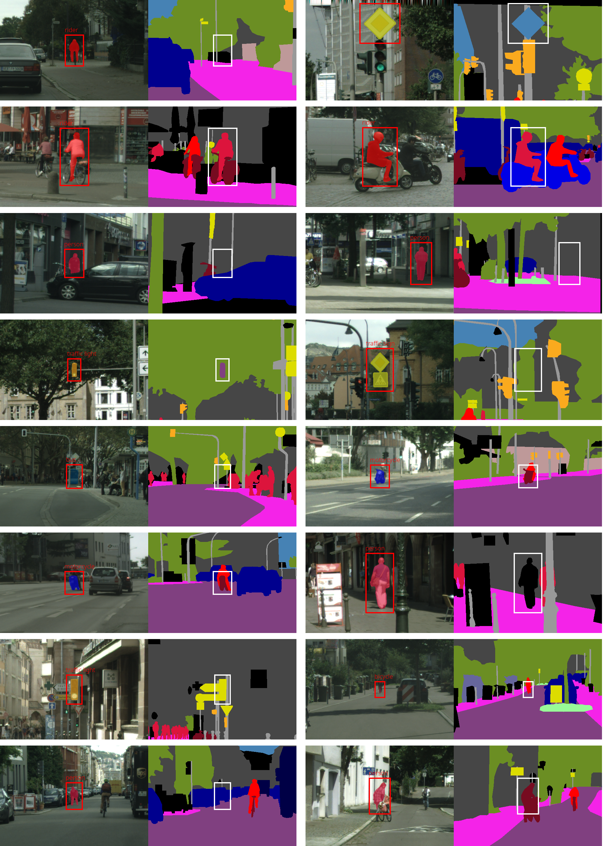
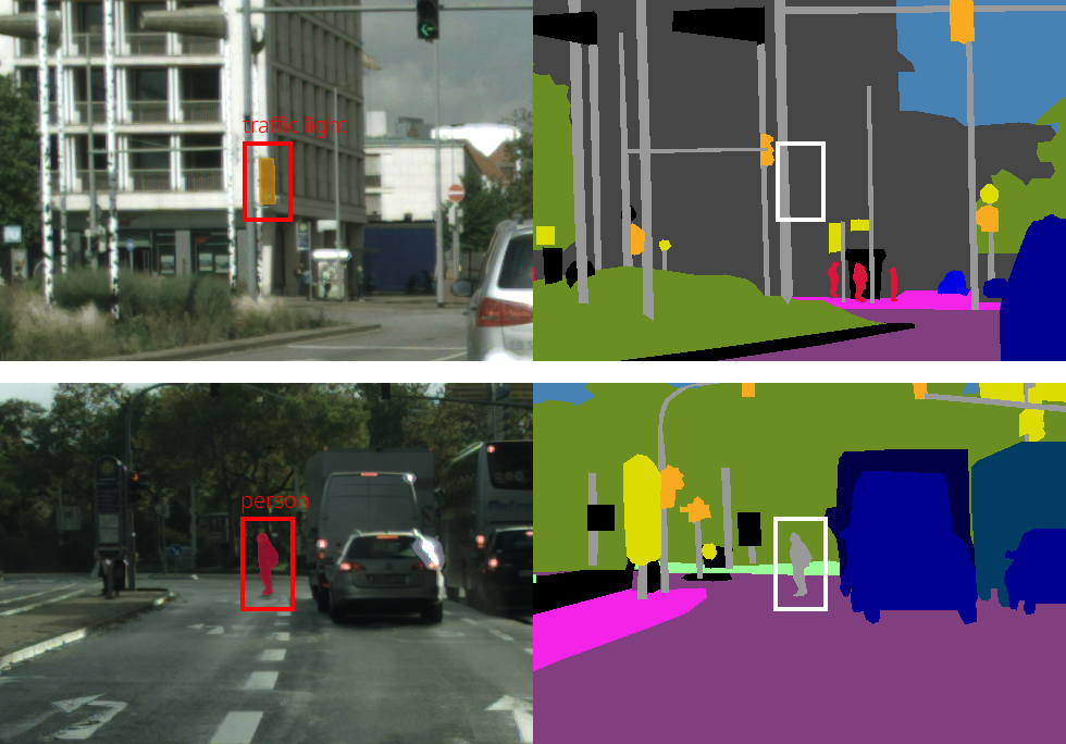
On the validation set our method achieves a precision of $53\%$ where we found $106$ label errors when considering $200$ candidates. The results for the validation set are a slightly inferior compared to the results for the training set which is to be expected as the validation set only contains $500$ images while we examine the same amount of discoveries from our method. For a class-wise breakdown of these results, see table 8 in appendix C. Two examples of identified label errors are presented in fig. 2.

Dataset	$\mathrm{mIoU}$	$\mathrm{TP}$	$\mathrm{FP}$	$\mathrm{Prec}$
Cityscapes Training	86.82	115	85	57.50
Cityscapes Validation	86.82	106	94	53.00
PascalVOC Validaiton	78.03	95	105	47.50
Coco Validation	28.20	134	66	67.00
ADE20K	43.12	110	90	55.00

Table 5: Precision of our approach for different datasets.

Summarizing the Cityscapes results, by reviewing only $400$ candidates conservatively, we already identified $231$ label errors. The precision of $53\%$ for the small validation set indicates that there may remain further label errors which can be approached further by using our method.

Figure 2: Two examples of label errors detected by our method, one example per row. Left: prediction of our label error detection method; right: “ground truth” annotation. Our method is able to find both, overlooked and flipped labels.

Results on PascalVOC.

The PASCAL Visual Object Classes (VOC) 2012 dataset [12] contains $20$ object categories of a wide variety. The training set consists of $8497$ and the validation set of $2857$ images. The attention net achieves a $\mathrm{mIoU}$ of $78.03\%$ on the validation set. For the current and all subsequent datasets, we only study the validation set as we expect a vast amount of label errors therein. Conversely to Cityscapes, we do not additionally filter or split the classes. For the evaluation, we consider every class and again examine the $200$ candidates with highest meta classification probability.

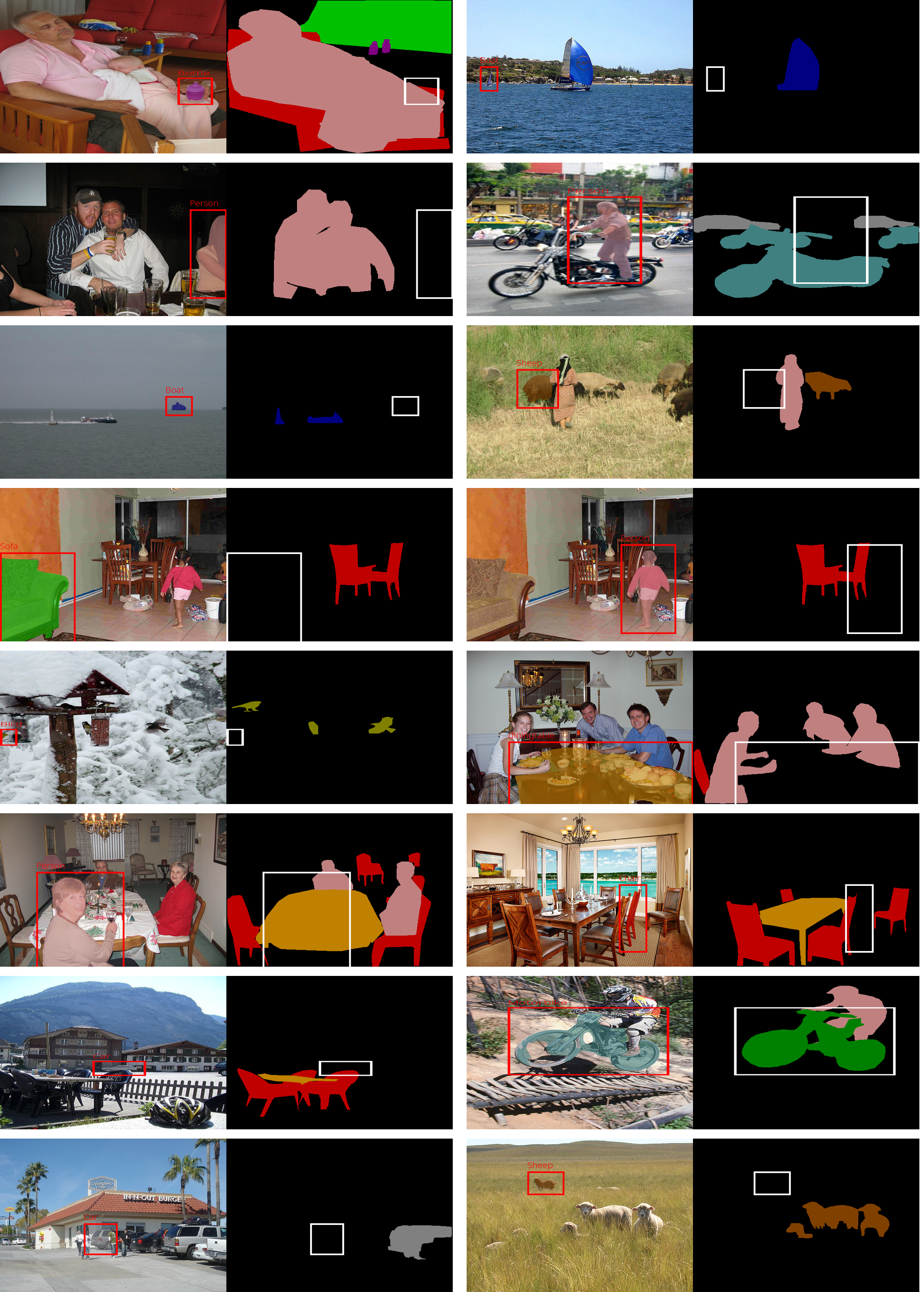
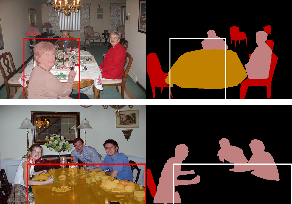
We identified $95$ label errors and obtained a precision of $47.5\%$; see table 5. One might expect that a high $\mathrm{IoU}$ for a specific class would result in a high precision for this class. However, our results contradicts this intuition. While this is true for the class of Person for which we achieve a precision of $84\%$, the opposite is true for almost every other class. For a detailed discussion on these results we refer to appendix C. Two exemplary label errors are shown in fig. 3

Figure 3: Two detected label errors in PascalVOC. The visualization scheme follows the one of fig. 2.

Results on COCO-Stuff.

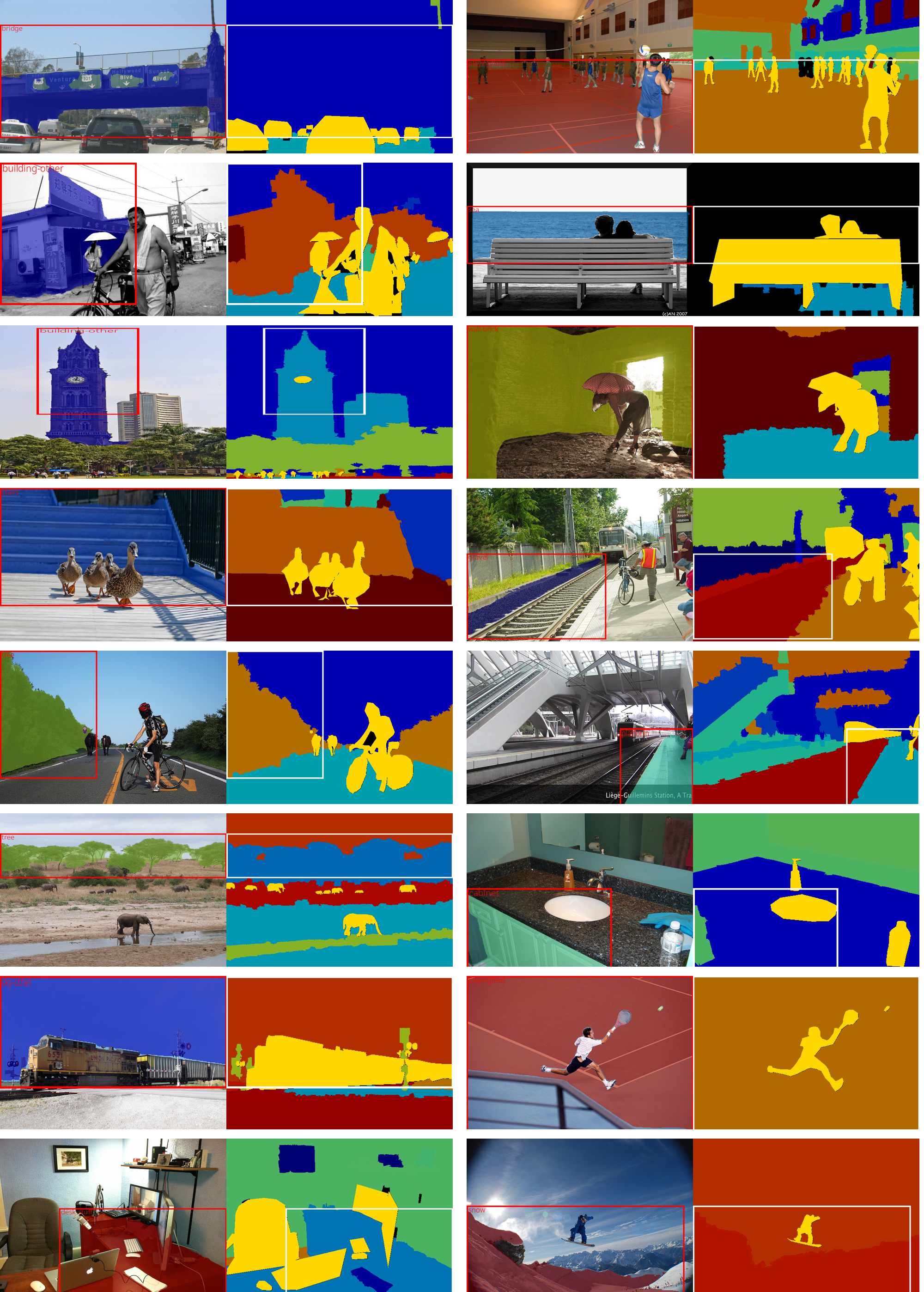
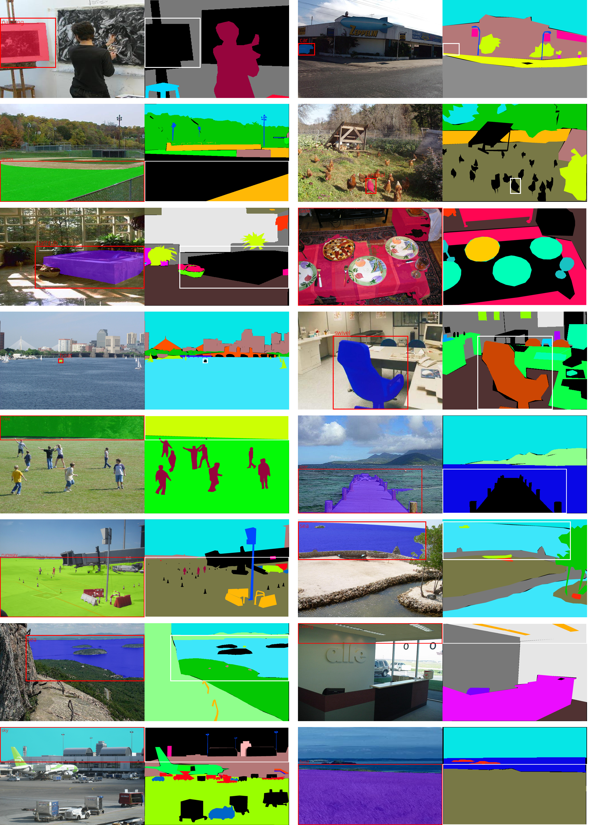
The COCO-Stuff dataset [1] is the largest dataset we examine, containing $118$K training images and $5$K validation images of variable size and $93$ total categories. On the validation set, the net achieves an $\mathrm{mIoU}$ of $28.20\%$ and our approach obtained a high precision of $67\%$. This amounts to $134$ true positives within $200$ candidates from $36$ class. For this dataset we also observed that a low $\mathrm{IoU}$ does not automatically imply a low precision. Again we refer to appendix C for more details. Note that for this dataset we were not able find a documentation that specifies the annotation policy precisely. Therefore, in our evaluation, we used the class descriptions.

Results on ADE20K.

ADE20K [47, 46] consists of $27$K images annotated in $151$ classes. We trained for $200$ epochs and a crop size of $600\times 600$ pixels on $25$K training images and applied our method to the validation set of $2$K images, where we obtain a precision $52.5\%$ with an $\mathrm{mIoU}$ of $43.12\%$. Table 5 shows the results for this dataset. For the further details see appendix C. We found $104$ label errors in $200$ predictions across $58$ classes. We note that the class definitions of this dataset are in part not sufficiently distinct. In addition, since we were not able to find class descriptions for this dataset, we had to infer from the ground truth annotation which objects the classes represent. This led to a significant amount of false positives since we were regularly not able to evaluate confidently whether the prediction is a true positive or not.

6 Conclusion & Outlook

In this work, we demonstrated how uncertainty quantification leverages the detection of label errors in semantic segmentation datasets via deep learning. We find good trade-offs of human labor and discovery rates of label errors, therefore enabling the efficient quality improvement for semantic segmentation datasets. In the future, we plan to develop measures and estimators for overall dataset quality. Furthermore, we plan to extend our method to detect falsely induced connected components (e.g. a piece of sky within the street) that are likely to be overlooked by the DNN, thus probably being overlooked by our method. We make our codes for benchmark, evaluation and method publicly available under GitHub.

x

Appendix A Details on Dataset Creation and the Injection of Label Errors

CARLA.

Figure 4: Two annotations, before and after we applied smoothing. Note that, we do not smooth every class. Smoothing is applied onto the classes of pedestrians, poles, vegetation and vehicles. Additionally, we remove road lines from the annotation.

We create the dataset by randomly selecting a spawn point of the ego vehicle and recording in the first step a segmentation mask of the empty scene. We then randomly spawn objects around the ego vehicle and record an rgb image as well as another segmentation mask of the scene, while all objects including the ego vehicle are static. The latter pair of image and ground truth serve as input image and unperturbed / clean reference ground truth for evaluation. Thereafter, we copy the connected component of the clean annotation mask into the first one and randomly select components to omit in order to induce label errors. When recording the same scene multiple times in CARLA, the ground truth typically varies at boundaries of connected components due to rendering effects. Our procedure of ground truth generation avoids this effect.

The CARLA simulator’s semantic segmentation sensor provides very precised annotated segmentation masks. To emulate human annotated masks and to make our synthetic dataset more realistic, we smooth these masks in order to reduce the degree of detailedness. We proceed class by class and consider the classes of Pedestrians, Poles, Vegetation, and Vehicles (in arbitrary order). More precisely, our smoothing process proceeds as follows: For a given street scene, we first create binary maps for each class where every pixel of the class under consideration for smoothing obtains some value $i\in\mathbb{N}$ and we associate $0$ to every other pixel. The value $i$ enables us to control how much an object is smoothed. For our smoothing we set $i=10$. We then apply a Gaussian smoothing kernel onto the binary masks and use these smoothed binary masks as index map to overwrite the values of the corresponding pixels in the original segmentation mask with the currently smoothed class value. To avoid that we override values of pixels that belong to a component that is in fact in front (in terms of visual depth) of a component of the smoothed class, we use depth information provided by CARLA to determine during smoothing for each pixel which class is in front. After we finished this smoothing process we fill the windows of vehicles in the scene as CARLA ignores them in the labeling process. Lastly, we remove the road lines and overwrite them with the class road. The result of this process can be seen in fig. 4.

Cityscapes.

Due to the availability of polygonal annotations and the labeling style being hierarchical (objects are mostly labeled on top of the background components), we can drop polygons according to the procedure mentioned in eq. 3. In this way, we obtain a perturbed ground truth by dropping polygons and then generating the pixel-wise segmentation masks. Although the labeling style is hierarchical, it is possible that the removal of a polygon in the annotation leads to an unlabeled region in the resulting perturbed mask. As it turned out in section 5, this is a realistic error and therefore we do not ignore unlabeled components in our evaluation but consider them as a class in the dataset.

Appendix B A Class-wise Breakdown of Results for Induced Label Errors.

In this section we present the class-wise results for Cityscapes in experiment $1$ with pertubation rate $\hat{p}=0.5$ using the sota weights for Nvidia’s multiscale attention net (table 6) and for the Deeplab net (table 7). Ignoring the class Bus, for the attention net we obtained the best $\mathrm{F1}$ score for the class Person with $74.88\%$ which also contains the most label errors. The lowest $\mathrm{F1}$ scores occur for the classes Traffic Light and Traffic Sign. From a visual inspection of predicted masks, it seems that the DNN relies more on the geometry of these objects, while paying less attention to their textures. Similarly, for the Deeplab architecture the class Person achieves the second highest $\mathrm{F1}$ score with $76.64\%$. Here, the best class is Rider with $80.39\%$ which has a $\mathrm{F1}$ score of only $58.99\%$ with Nvidia’s net. The lowest scores are again given for class Traffic Light and class Traffic Sign.

	$\mathrm{(m)IoU}$	$\mathrm{TP}$	$\mathrm{FN}$	$\mathrm{FP}$	$\mathrm{Prec}$	$\mathrm{Rec}$	$\mathrm{F1}$
Bicycle	84.26	81	44	26	75.70	64.80	69.83
Bus	95.48	1	0	1	50.00	100.00	66.67
Car	96.86	100	61	56	64.10	62.11	63.09
Motorcycle	78.24	8	6	0	100.00	57.14	72.73
Person	87.91	161	76	32	83.42	67.93	74.88
Rider	75.47	41	46	11	78.85	47.13	58.99
Traffic Light	79.88	38	1	63	37.62	97.44	54.29
Traffic Sign	87.64	55	17	179	23.50	76.39	35.05
Truck	92.64	2	8	3	35.59	20.00	26.67
Overall	86.82	487	259	371	56.76	65.28	60.72

Table 6: Class-wise results for Cityscapes using the Nvidia’s Multiscale Attention net.

	$\mathrm{(m)IoU}$	$\mathrm{TP}$	$\mathrm{FN}$	$\mathrm{FP}$	$\mathrm{Prec}$	$\mathrm{Rec}$	$\mathrm{F1}$
Bicycle	79.00	76	49	24	76.00	60.80	67.56
Bus	94.00	1	0	0	100.00	100.00	100.00
Car	96.50	102	59	29	77.86	63.35	69.86
Motorcycle	73.80	7	7	1	87.50	50.00	63.64
Person	88.20	159	78	19	89.33	67.09	76.63
Rider	75.40	43	44	2	95.56	49.43	80.39
Traffic Light	79.00	33	6	44	62.86	84.62	56.90
Traffic Sign	82.80	56	16	206	21.37	77.78	33.53
Truck	78.80	4	6	0	100.00	40.00	57.14
Overall	81.40	481	265	325	59.68	64.48	61.98

Table 7: Class-wise results for Cityscapes using the Deeplab net.

Appendix C Class-wise Breakdown of Found Label Errors in Frequently used Datasets

This section is an extension to the discussion of section 5.2. Here we provide additional details for each dataset we studied and present results for selected classes. In appendix D we present for each dataset a collection of label errors found in the respective datasets.

Cityscapes.

Figure 5: The connected component shown here is originally labeled as void. Our method predicts a label error here which is likely true. However, since we cannot confirm this without any doubt we validated it as false positive.

In table 8 we have given the class-wise results for Cityscapes and fig. 7 presents example errors we found. In the training set we have found $106$ label errors by reviewing $200$ predictions. For the classes of person, rider/bicycle and vehicles altogether we found $90$ true positives, $60$ false positive, obtaining a precision of $60\%$. For traffic lights and road signs we achieve a precision of $50\%$ by finding $25$ label errors in $50$ predictions. Apart from the class bus which only consists of one prediction, we observe the highest precision for the class rider with $88.89\%$ while, at the same time the $\mathrm{IoU}$ is the lowest of all predicted classes with $75.47\%$. This indicates that our approach does not necessarily depend on a high $\mathrm{IoU}$. It is also possible that the computed $\mathrm{IoU}$ for this class is dragged down by label errors in this class. The most errors we found for this class were caused by labeling a rider as a person.

We observed the same for the validation set. Combining the results of the classes of person, rider/bicycle and vehicles we have a precision of $55.33\%$ and of $46.00\%$ for classes of traffic lights and road signs. The result are slightly worse, which is to be expected as the validation set only consists of $500$ images while the training set includes almost $3000$ images.

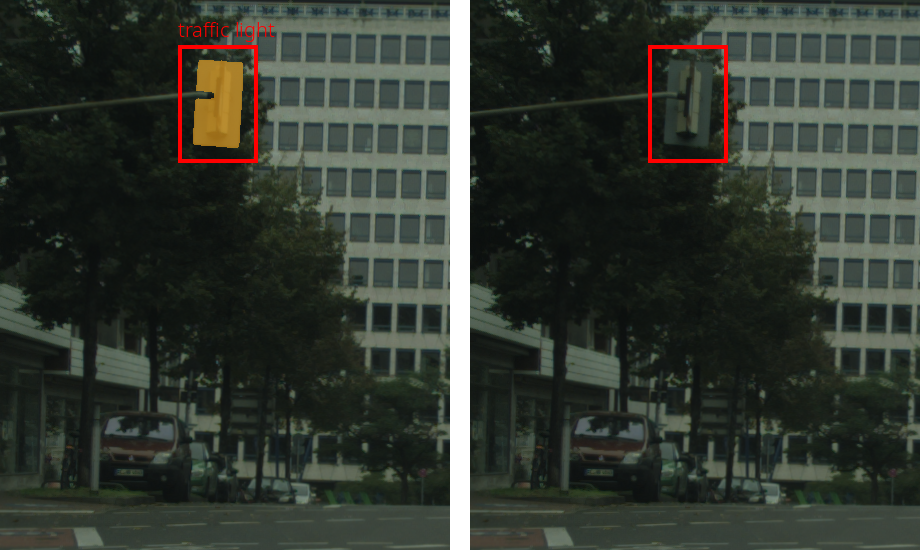
Due to our conservative validation approach, for the class traffic light we validated several predictions as false positive even though they could be viewed as true positives; see fig. 5 for examples.

Validating them as true positive would result in additional $15$ true positives and a precision of $93\%$ for the class of traffic lights and of $65\%$ in total. Also, in fig. 6 we present a case that occurred several times and is debatable whether it is a false or true positives. However, following the official Cityscapes labeling policy and to avoid any confusion, we consider them to be false positives.

Figure 6: The DNN has correctly found a car component here. However, it is not a foreground object and therefore labeled as void in the ground truth. According to the labeling policy this is a false positive.

Training set					Validation set
Class	$\mathrm{(m)IoU}$	$\mathrm{TP}$	$\mathrm{FP}$	$\mathrm{Prec}$	$\mathrm{TP}$	$\mathrm{FP}$	$\mathrm{Prec}$
Bicycle	84.26	16	8	66.67	16	8	66.67
Bus	95.48	1	0	100.00	2	3	40.00
Car	96.86	13	36	26.53	30	32	48.39
Motorcycle	78.24	2	1	66.67	0	0	NaN
Person	87.91	34	17	66.67	35	13	72.91
Rider	75.47	16	2	88.89	7	2	77.78
Traffic sign	79.88	10	18	35.71	12	17	41.38
Traffic light	87.64	13	9	59.09	13	8	61.90
Truck	92.64	1	3	25.00	0	2	00.00
Overall	86.82	106	94	53.00	115	85	57.50

Table 8: Classwise results for the train (left) and validation (right) sets of Cityscapes.

PascalVOC					COCO-Stuff					ADE20K
Class	$\mathrm{(m)IoU}$	$\mathrm{TP}$	$\mathrm{FP}$	$\mathrm{Prec}$	Class	$\mathrm{(m)IoU}$	$\mathrm{TP}$	$\mathrm{FP}$	$\mathrm{Prec}$	Class	$\mathrm{(m)IoU}$	$\mathrm{TP}$	$\mathrm{FP}$	$\mathrm{Prec}$
Bicycle	78.78	0	5	00.00	Building-other	30.81	16	7	69.57	Building	83.89	0	17	00.00
Boat	66.76	4	3	57.14	Ceiling-other	93.76	5	2	71.42	Cabinet	65.40	4	2	66.67
Bottle	81.18	5	6	45.45	Desk-stuff	66.83	4	0	100.00	Chair	57.72	3	3	50.00
Car	83.64	8	8	50.00	Grass	90.81	11	6	64.71	Coffee	64.15	6	0	100.00
Cat	89.21	1	10	09.09	Pavement	26.77	3	3	50.00	Floor	80.32	28	5	84.85
Chair	51.97	17	11	60.71	Playingfield	44.87	9	0	100.00	Grass	59.71	1	5	16.67
Dining table	51.47	10	6	62.50	River	85.00	1	1	50.00	House	25.05	0	3	00.00
Dog	85.01	0	14	00.00	Road	90.70	2	2	50.00	Painting	73.64	1	4	20.00
Person	85.79	38	7	84.44	Sea	96.65	3	2	60.00	Sea	47.57	5	1	83.33
Potted plant	68.02	0	4	00.00	Sky-other	63.13	17	2	89.47	Ship	4.58	2	3	40.00
Sheep	79.61	2	3	40.00	Snow	97.21	6	2	75.00	Sky	92.79	6	3	66.67
Sofa	52.02	6	9	40.00	Table	00.00	0	6	00.00	Table	59.24	4	1	80.00
Train	82.94	1	5	16.67	Tree	73.33	31	9	77.50	Tree	73.58	3	1	75.00
Tv monitor	68.67	0	5	00.00	Wall-concrete	58.59	9	11	45.00	Wall	75.24	7	12	36.84
Overall	78.03	95	105	47.50	Overall	28.20	134	66	67.00	Overall	43.12	110	90	55.00

Table 9: Classwise results for the validation set of PascalVOC, COCO, and ADE20K.

PascalVOC.

For PascalVOC, COCO, and ADE20K we presented a selection of the most informative classes in table 9. Examples errors are shown in fig. 8. At first glance, one might expect that classes with low $\mathrm{IoU}$ are difficult for our label error detection. PascalVOC provides several counter example for this. While for the class Person we observe high $\mathrm{IoU}$ scores together with strong label error detection performance, considering the overall picture there is a clear anti-correlation between label error detection performance and $\mathrm{IoU}$ for PascalVOC. Even with low IoU scores, our method is still able to find label errors. For example, the DNN exhibits a comparatively low $\mathrm{IoU}$ score of $51.97\%$ for the chair class but still our method found $17$ label errors with a precision of $61\%$. We observe the same for the class Dining table in which we found $10$ label errors with a precision of $0.63$ and an $\mathrm{IoU}$ of $51.47$. Calculating the Pearson correlation between the IoU and the precision scores we obtain a low negative value of $-0.27$. Altogether, the findings indicate that the low $\mathrm{mIoU}$ might be partially caused by a poor label quality of the dataset.

COCO.

Selected class results are given in table 9 and some errors are presented in fig. 9. The best results are achieved for the classes of Building-other, Grass, Playingfield, Sky-other and Tree with precision scores significantly above $50\%$ and a representative amount of predictions. Overall, for this dataset we achieved the highest precision of $67\%$ in $200$ prediction across $36$ predicted classes. For this dataset we also can observe the IoU and precision scores also seem to be barley correlated. This observation is supported by a low correlation score of $0.36$.

ADE20K.

In this dataset we found $104$ label errors in $200$ predictions across $58$ classes. Table 9 shows results for selected classes and fig. 10 some example errors. As we already mentioned the class definitions of this dataset are in part not sufficiently distinct. In addition, since we were not able to find class descriptions for this dataset, we inferred from the ground truth annotation which objects the classes represent. This led to a significant amount of false positives since we were oftentimes unable to assign $\mathrm{TP}$ with appropriate confidence. This applies in particular to the class “building”. In ADE20K, there also exists a class named house which seems to accommodate buildings for human habitation. For the DNN it is difficult to distinguish these two classes, hence it predicts most of the buildings/houses as buildings This leads to a high $\mathrm{IoU}$ for the class building, a low $\mathrm{IoU}$ of $25.05$ for the class house, and a precision of $0\%$ for the building class. However, despite the mentioned issues, the results for ADE20K are comparable to those obtained for the other datasets. Also for this dataset we have a low correlation score of $0.19$.

Appendix D Additional Examples of label Errors in Frequently used Datasets

Below we present collages of examplary label errors we found in the datasets discussed in the previous section. Each collage contains $16$ pairs of images where each pair represent one label error. The right image represents a section of the ground truth segmentation mask and the left image displays a missed or flipped component. Figures 7, 8, 9 and 10 are collections of label errors in Cityscapes, PascalVOC, COCO-Stuff and ADE20K, respectively.

Figure 7: A collection of label errors present in Cityscapes. Left: prediction of our label error detection method; right: “ground truth” annotation. Our method is able to find both, overlooked and flipped labels.

Figure 8: A collection of label errors present in PascalVOC. The visualization scheme follows the one of fig. 7.

Figure 9: A collection of label errors present in COCO-Stuff. The visualization scheme follows the one of fig. 7.

Figure 10: A collection of label errors present in ADE20K. The visualization scheme follows the one of fig. 7.

References

- [1] Holger Caesar, Jasper R. R. Uijlings, and Vittorio Ferrari. Coco-stuff: Thing and stuff classes in context. CoRR, abs/1612.03716, 2016.
- [2] Robin Chan, Krzysztof Lis, Svenja Uhlemeyer, Hermann Blum, Sina Honari, Roland Siegwart, Mathieu Salzmann, Pascal Fua, and Matthias Rottmann. Segmentmeifyoucan: A benchmark for anomaly segmentation. CoRR, abs/2104.14812, 2021.
- [3] Robin Chan, Matthias Rottmann, Fabian Hüger, Peter Schlicht, and Hanno Gottschalk. Controlled false negative reduction of minority classes in semantic segmentation. In 2020 International Joint Conference on Neural Networks, IJCNN 2020, Glasgow, United Kingdom, July 19-24, 2020, pages 1–8. IEEE, 2020.
- [4] Liang-Chieh Chen, Yukun Zhu, George Papandreou, Florian Schroff, and Hartwig Adam. Encoder-decoder with atrous separable convolution for semantic image segmentation. ArXiv, abs/1802.02611, 2018.
- [5] Pengfei Chen, Benben Liao, Guangyong Chen, and Shengyu Zhang. Understanding and utilizing deep neural networks trained with noisy labels. International Conference on Machine Learning (ICML), 2019.
- [6] Pascal Colling, Lutz Roese-Koerner, Hanno Gottschalk, and Matthias Rottmann. Metabox+: A new region based active learning method for semantic segmentation using priority maps. In Proceedings of the 10th International Conference on Pattern Recognition Applications and Methods - Volume 1: ICPRAM,, pages 51–62. INSTICC, SciTePress, 2021.
- [7] Pascal Colling, Matthias Rottmann, Lutz Roese-Koerner, and Hanno Gottschalk. False positive detection and prediction quality estimation for lidar point cloud segmentation. In 2021 IEEE 33rd International Conference on Tools with Artificial Intelligence (ICTAI), pages 18–25. IEEE, 2021.
- [8] Marius Cordts, Mohamed Omran, Sebastian Ramos, Timo Rehfeld, Markus Enzweiler, Rodrigo Benenson, Uwe Franke, Stefan Roth, and Bernt Schiele. The cityscapes dataset for semantic urban scene understanding. In Proc. of the IEEE Conference on Computer Vision and Pattern Recognition (CVPR), 2016.
- [9] Markus Dickinson. Detection of annotation errors in corpora. Language and Linguistics Compass, 9(3):119–138, 2015.
- [10] Alexey Dosovitskiy, Germán Ros, Felipe Codevilla, Antonio M. López, and Vladlen Koltun. CARLA: an open urban driving simulator. CoRR, abs/1711.03938, 2017.
- [11] Alexey Dosovitskiy, Germán Ros, Felipe Codevilla, Antonio M. López, and Vladlen Koltun. Carla: An open urban driving simulator. ArXiv, abs/1711.03938, 2017.
- [12] Mark Everingham, S. M. Ali Eslami, Luc Van Gool, Christopher K. I. Williams, John M. Winn, and Andrew Zisserman. The pascal visual object classes challenge: A retrospective. International Journal of Computer Vision, 111:98–136, 2014.
- [13] Di Feng, Christian Haase-Schutz, Lars Rosenbaum, Heinz Hertlein, Claudius Glaser, Fabian Timm, Werner Wiesbeck, and Klaus Dietmayer. Deep multi-modal object detection and semantic segmentation for autonomous driving: Datasets, methods, and challenges. IEEE Transactions on Intelligent Transportation Systems, 22(3):1341–1360, mar 2021.
- [14] Jacob Goldberger and Ehud Ben-Reuven. Training deep neural-networks using a noise adaption layer. International Conference on Learning Representations (ICLR), 2017.
- [15] Bo Han, Quanming Yao, Xingrui Yu, Gang Niu, Miao Xu, Weihua Hu, Ivor W. Tsang, and Masashi Sugiyama. Co-teaching: Robust training of deep neural networks with extremely noisy labels. Conference on Neural Information Processing Systems (NeurIPS), 2018.
- [16] Nicholas Heller, Joshua Dean, and Nikolaos Papanikolopoulos. Imperfect segmentation labels: How much do they matter? Intravascular Imaging and Computer Assisted Stenting and Large-Scale Annotation of Biomedical Data and Expert Label Synthesis, 2018.
- [17] Dan Hendrycks, Mantas Mazeika, and Duncan Wilson. Using trusted data to train deep networks on labels corrupted by severe noise. Conference on Neural Information Processing Systems (NeurIPS), 2018.
- [18] Katharina Hoebel, Vincent Andrearczyk, Andrew Beers, Jay Patel, Ken Chang, Adrien Depeursinge, Henning Müller, and Jayashree Kalpathy-Cramer. An exploration of uncertainty information for segmentation quality assessment. In Ivana Išgum and Bennett A. Landman, editors, Medical Imaging 2020: Image Processing, volume 11313, pages 381 – 390. International Society for Optics and Photonics, SPIE, 2020.
- [19] Rasheed Hussain and Sherali Zeadally. Autonomous cars: Research results, issues, and future challenges. IEEE Communications Surveys & Tutorials, 21:1275–1313, 2019.
- [20] Lu Jiang, Zhengyuan Zhou, Thomas Leung, Li-Jia Li, and Li Fei-Fei. Mentornet: Learning data-driven curriculum for very deep neural networks on corrupted labels. International Conference on Machine Learning (ICML), 2018.
- [21] Konstantinos Kamnitsas, Christian Ledig, Virginia F.J. Newcombe, Joanna P. Simpson, Andrew D. Kane, David K. Menon, Daniel Rueckert, and Ben Glocker. Efficient multi-scale 3d CNN with fully connected CRF for accurate brain lesion segmentation. Medical Image Analysis, 36:61–78, feb 2017.
- [22] Tejaswi Kasarla, G Nagendar, Guruprasad M. Hegde, V. Balasubramanian, and C.V. Jawahar. Region-based active learning for efficient labeling in semantic segmentation. In 2019 IEEE Winter Conference on Applications of Computer Vision (WACV), pages 1109–1117, 2019.
- [23] Simon Kohl, Bernardino Romera-Paredes, Clemens Meyer, Jeffrey De Fauw, Joseph R. Ledsam, Klaus Maier-Hein, S. M. Ali Eslami, Danilo Jimenez Rezende, and Olaf Ronneberger. A probabilistic u-net for segmentation of ambiguous images. In S. Bengio, H. Wallach, H. Larochelle, K. Grauman, N. Cesa-Bianchi, and R. Garnett, editors, Advances in Neural Information Processing Systems, volume 31. Curran Associates, Inc., 2018.
- [24] Sampo Kuutti, Richard Bowden, Yaochu Jin, Phil Barber, and Saber Fallah. A survey of deep learning applications to autonomous vehicle control. CoRR, abs/1912.10773, 2019.
- [25] Alexander Selvikvåg Lundervold and Arvid Lundervold. An overview of deep learning in medical imaging focusing on mri. Zeitschrift für Medizinische Physik, 29(2):102–127, 2019. Special Issue: Deep Learning in Medical Physics.
- [26] Kira Maag, Matthias Rottmann, and Hanno Gottschalk. Time-dynamic estimates of the reliability of deep semantic segmentation networks. In IEEE International Conference on Tools with Artificial Intelligence (ICTAI), 11 2020.
- [27] Curtis G. Northcutt, Anish Athalye, and Jonas Mueller. Pervasive label errors in test sets destabilize machine learning benchmarks. arXiv preprint arXiv:2103.14749, 2021.
- [28] Curtis G. Northcutt, Lu Jiang, and Isaac L. Chuang. Confident learning: Estimating uncertainty in dataset labels. Journal of Artificial Intelligence Research, 2019.
- [29] Ozan Oktay, Jo Schlemper, Loïc Le Folgoc, M. J. Lee, Mattias P. Heinrich, Kazunari Misawa, Kensaku Mori, Steven G. McDonagh, Nils Y. Hammerla, Bernhard Kainz, Ben Glocker, and Daniel Rueckert. Attention u-net: Learning where to look for the pancreas. ArXiv, abs/1804.03999, 2018.
- [30] Scott E. Reed, Honglak Lee, Dragomir Anguelov, Christian Szeged, Dumitru Erhan, and Andrew Rabinovich. Training deep neural networks on noisy labels with bootstrapping. International Conference on Learning Representations (ICLR), 2015.
- [31] Matthias Rottmann, Pascal Colling, Thomas-Paul Hack, Robin Chan, Fabian Hüger, Peter Schlicht, and Hanno Gottschalk. Prediction error meta classification in semantic segmentation: Detection via aggregated dispersion measures of softmax probabilities. In 2020 International Joint Conference on Neural Networks, IJCNN 2020, Glasgow, United Kingdom, July 19-24, 2020, pages 1–9. IEEE, 2020.
- [32] Matthias Rottmann and Marius Schubert. Uncertainty measures and prediction quality rating for the semantic segmentation of nested multi resolution street scene images. In IEEE Conference on Computer Vision and Pattern Recognition Workshops, CVPR Workshops 2019, Long Beach, CA, USA, June 16-20, 2019, pages 1361–1369. Computer Vision Foundation / IEEE, 2019.
- [33] Florian A. Schmidt. Crowdproduktion von trainingsdaten – zur rolle von online-arbeit beim trainieren autonomer fahrzeuge, 2019. Study der Hans-Böckler-Stiftung, Düsseldorf.
- [34] Burr Settles. Active learning literature survey. Computer Sciences Technical Report 1648, University of Wisconsin–Madison, 2009.
- [35] Ke Sun, Yang Zhao, Borui Jiang, Tianheng Cheng, Bin Xiao, Dong Liu, Yadong Mu, Xinggang Wang, Wenyu Liu, and Jingdong Wang. High-resolution representations for labeling pixels and regions. CoRR, abs/1904.04514, 2019.
- [36] Andrew Tao, Karan Sapra, and Bryan Catanzaro. Hierarchical multi-scale attention for semantic segmentation. ArXiv, abs/2005.10821, 2020.
- [37] Andrew Tao, Karan Sapra, and Bryan Catanzaro. Pytorch implementation of hierarchical multi-scale attention for semantic segmentation. https://github.com/NVIDIA/semantic-segmentation, 2021.
- [38] Agnieszka Tomczack, Nassir Navab, and Shadi Albarqouni. Learn to estimate labels uncertainty for quality assurance. CoRR, abs/1909.08058, 2019.
- [39] Yisen Wang, Xingjun Ma, Zaiyi Chen, Yuan Luo, Jinfeng Yi, and James Bailey. Symmetric cross entropy for robust learning with noisy labels. International Conference on Computer Vision (ICCV), 2019.
- [40] Zifeng Wu, Chunhua Shen, and Anton van den Hengel. Wider or deeper: Revisiting the resnet model for visual recognition. Pattern Recognition, 90:119–133, 2019.
- [41] Yilun Xu and Peng Cao. Novel information-theoretic loss function for training deep nets robust to label noise. Conference on Neural Information ProcessingSystems (NeurIPS), 2019.
- [42] Rumeng Yi, Yaping Huang, Qingji Guan, Mengyang Pu, and Runsheng Zhang. Learning from pixel-level label noise: A new perspective for semi-supervised semantic segmentation. IEEE Transactions on Image Processing, 31:623–635, 2022.
- [43] Hongyi Zhang, Moustapha Cisse, Yann N. Dauphin, and David Lopez-Paz. mixup: Beyond empirical risk minimization. International Conference on Learning Representations (ICLR), 2018.
- [44] Le Zhang, Ryutaro Tanno, Kevin Bronik, Chen Jin, Parashkev Nachev, Frederik Barkhof, Olga Ciccarelli, and Daniel C. Alexander. Learning to segment when experts disagree. In Anne L. Martel, Purang Abolmaesumi, Danail Stoyanov, Diana Mateus, Maria A. Zuluaga, S. Kevin Zhou, Daniel Racoceanu, and Leo Joskowicz, editors, Medical Image Computing and Computer Assisted Intervention – MICCAI 2020, pages 179–190, Cham, 2020. Springer International Publishing.
- [45] Le Zhang, Ryutaro Tanno, Mou-Cheng Xu, Chen Jin, Joseph Jacob, Olga Ciccarelli, Frederik Barkhof, and Daniel C. Alexander. Disentangling human error from the ground truth in segmentation of medical images. CoRR, abs/2007.15963, 2020.
- [46] Bolei Zhou, Hang Zhao, Xavier Puig, Sanja Fidler, Adela Barriuso, and Antonio Torralba. Scene parsing through ade20k dataset. In Proceedings of the IEEE Conference on Computer Vision and Pattern Recognition, 2017.
- [47] Bolei Zhou, Hang Zhao, Xavier Puig, Tete Xiao, Sanja Fidler, Adela Barriuso, and Antonio Torralba. Semantic understanding of scenes through the ade20k dataset. International Journal of Computer Vision, 127(3):302–321, 2019.
- [48] Yi Zhu, Karan Sapra, Fitsum A. Reda, Kevin J. Shih, Shawn D. Newsam, Andrew Tao, and Bryan Catanzaro. Improving semantic segmentation via video propagation and label relaxation. CoRR, abs/1812.01593, 2018.