Marginally deformed Schrödinger/dipole CFT correspondence

Abstract

We construct and thoroughly study a new integrable example of the AdS/CFT correspondence with Schrödinger symmetry. On the gravity side, the supergravity solution depends on two parameters and is obtained by marginally deforming the internal space of the Schrödinger background through a series of TsT transformations. On the field theory side, we identify the dual field theory which also depends on two parameters.

We find a point-like string solution and derive its dispersion relation. A non-trivial test of the correspondence is provided by using the Landau-Lifshitz coherent state approach to reproduce the leading, in the deformation parameters, terms of that relation. Then, we calculate the Wilson loop, describing the quark/anti-quark potential at strong coupling. It exhibits confining behaviour when the separation length is much less than the Schrödinger parameter. When the separation length is much greater than the Schrödinger parameter the behaviour is that of a conformal theory. Subsequently, we take the Penrose limit along a certain null geodesic of the constructed background and calculate the bosonic spectrum. Based on that spectrum, we make an educated guess for the exact, in the ’t Hooft coupling, dispersion relation of the magnon excitations in the original doubly deformed background. This provides us with an exact prediction for the dimensions of the dual field theory operators.

1 Introduction

One of the most fascinating discoveries in theoretical physics is the so-called AdS/CFT correspondence Maldacena:1997re . In its original form it asserts the complete equivalence between type-IIB string theory on the $AdS_{5}\times S^{5}$ background and the maximally supersymmetric gauge theory in 4 dimensions, namely $\mathcal{N}=4$ Super Yang-Mills (SYM). The importance of the correspondence relies on its weak/strong coupling nature which provides powerful tools in understanding the strongly coupled dynamics of gauge theories. One of the main properties of the correspondence is its integrability. Exploiting the key feature of integrability which both of the aforementioned theories possess, an intense activity took place allowing the determination of its spectrum, at the planar level, for any value of the ’t Hooft coupling $\lambda$. To achieve this goal a variety of integrability based techniques were employed, such as the asymptotic Bethe ansatz Staudacher:2004tk , the thermodynamic Bethe ansatz Ambjorn:2005wa , and the Y-system Gromov:2009tv .

On the contrary, much less is known about the structure constants of the theory. The main obstacle here, is that for the calculation of the three-point correlation functions the exact form of the eigenstates of the dilatation operator is needed Georgiou:2008vk ; Georgiou:2009tp ; Georgiou:2011xj . Systematic studies of three-point correlators involving BPS, as well as, non-BPS operators were performed in Okuyama:2004bd ; Roiban:2004va ; Alday:2005nd ; Georgiou:2012zj by computing the contributions arising from both the planar one-loop Feynman diagrams, as well as from the correct form of the one-loop eigenstates of the dilatation operator Georgiou:2012zj ; Georgiou:2009tp .

More recently, certain non-perturbative in nature methods for bootstrapping three-point correlation functions were developed in Escobedo:2010xs ; Jiang:2014mja ; Basso:2015zoa ; Kazama:2016cfl . In addition, by exploiting the AdS/CFT correspondence, three-point correlation functions involving three heavy states in the $SU(2)$ or the $SL(2)$ subsectors were calculated at strong coupling Kazama:2013qsa ; Kazama:2011cp . This was accomplished by evaluating the area of the corresponding minimal surface through Pohlmeyer reduction. Another front where significant progress has been made is the one where the three-point correlator involves two non-protected operators with large charges, which are dual to classical string solutions, and one light state. The strong coupling result for this kind of three-point functions can be obtained by integrating the vertex operator that describes the light state over the classical surface which corresponds to the free propagation of the heavy state from one point of the boundary of $AdS_{5}$ to another Zarembo:2010rr ; Costa:2010rz ; Roiban:2010fe ; Georgiou:2010an ; Georgiou:2011qk ; Bajnok:2016xxu .

There is another occasion in which one can extract useful information for both the spectrum and the structure constants of the theory. This is possible in a particularly interesting limit, called the BMN limit Berenstein:2002jq in which one focuses on the sector of operators with large $R$-charge. These operators are dual to string states propagating in the pp-wave limit of the $AdS_{5}\times S^{5}$ geometry. Different proposals concerning the form of the cubic string Hamiltonian had been put forward in Spradlin:2002ar ; Pankiewicz:2002tg ; DiVecchia:2003yp . In Dobashi:2004nm ; Lee:2004cq the issue of how to correctly relate the string amplitudes obtained from the pp-wave cubic Hamiltonian to the structure constants of the $\mathcal{N}=4$ SYM was finally settled. This was achieved by combining a number of results available from both the string and the field theory sides Georgiou:2004ty ; Georgiou:2003kt ; Georgiou:2003aa ; Chu:2002pd . It is precisely this limit that we will employ in section 7 in order to get information for the spectrum of the marginally deformed conformal field theory (CFT) with Schrodinger symmetry.

Despite the aforementioned unprecedented insights into the strongly coupled dynamics of gauge theories originating from the original AdS/CFT scenario, $\mathcal{N}=4$ SYM is far from QCD, the theory one would like to understand at low energies where the confinement of the quarks takes place. In recent years, the identification of integrable deformations of the original AdS/CFT correspondence has attracted significant attention. These come a step closer to more realistic gauge theories. One of the reasons is that due to the deformations supersymmetry may be completely or partially broken. A case where the effects of the deformation is more profound is the correspondence between a certain Schrödinger spacetime and its dual null-dipole deformed conformal field theory Maldacena:2008wh ; Herzog:2008wg ; Adams:2008wt . On the gravity side Alishahiha:2003ru the theory may be easily obtained from the $AdS_{5}\times S^{5}$ background through a solution generating technique known as TsT transformation. One starts by performing an Abelian T-duality along one of the isometries of the five-sphere $S^{5}$ followed by a shift along one of the light-like directions of the $AdS_{5}$ boundary. Finally a second T-duality along the coordinate of the sphere dualised initially must be performed. The background resulting from this procedure is the so-called $Sch_{5}\times S^{5}$ and for certain choices of the five sphere isometry is non-supersymmetric. The holographic dual field theory is, of course, also non-supersymmetric and realises the Schrödinger symmetry algebra as its symmetry group. The field theory dual can be straightforwardly obtained by introducing a certain $\star$-product among the fields of the $\mathcal{N}=4$ SYM Lagrangian. This $\star$-product can be identified with the corresponding Drinfeld–Reshetikhin twist of the underlying integrable structure of the undeformed parent theory, namely $\mathcal{N}=4$ SYM Beisert:2005if ; Ahn:2010ws ; Matsumoto:2015uja ; Kyono:2016jqy ; vanTongeren:2015uha . Consequently, the deformed theory is fully integrable at the planar level with its integrability properties being inherited from the parent $\mathcal{N}=4$ SYM.

In contradistinction to the original AdS/CFT scenario very few observables have been calculated in the deformed version of the correspondence. In particular, two, three and $n$-point correlation functions of scalar operators were calculated in Fuertes:2009ex and Volovich:2009yh using the gravity side of the correspondence. It is important to mention that all these operators were dual to point-like strings propagating in the $Sch_{5}\times S^{5}$ background. Extended dyonic giant magnon and spike solutions were found in Georgiou:2017pvi and their dispersion relations were determined (in Zoakos:2020gyb finite size corrections of those solutions were calculated). The existence of these solutions is in complete agreement with the fact that the theory remains integrable. In the same work an exact expression, as a function of the coupling $\lambda$, for the dimensions of the gauge operators dual to the giant magnon solution was conjectured. Subsequently, the Penrose limit around a certain null geodesic was utilised in Georgiou:2019lqh to study the spectrum of the bosonic strings in the light-cone and show that two of the eigenfrequencies of the bosonic spectrum derived are in complete agreement with the dispersion relation of the giant magnon solution in the original Schrodinger background Georgiou:2017pvi ; Georgiou:2018zkt . Inspired by the pp-wave spectrum an improved conjecture about the exact in the t’Hooft coupling dispersion relation for the magnons in the original Schrödinger background was put forward. Furthermore, agreement was found between this dispersion relation and the one-loop anomalous dimension of BMN-like operators providing further evidence in favour of the correspondence. On the field theory side, the one-loop spectrum of operators belonging in a $SL(2)$ closed sub-sector has been determined in Guica:2017mtd . These authors found agreement between the one-loop anomalous dimensions of certain long operators and the string theory prediction (see also Ouyang:2017yko ).

Subsequently, three-point functions involving two heavy and one light operator were calculated in the Schrödinger background by the use of holography Georgiou:2018zkt . The light operator was chosen to be the dilaton while the heavy states were either the giant magnon or spike solutions constructed in Georgiou:2017pvi . These results are the first in the literature where three-point correlation functions involving heavy states described by extended string solutions were calculated. The results of Georgiou:2018zkt provide the leading term of the correlators in the large $\lambda$ expansion and are in perfect agreement with the form of the correlator as this is dictated by non-relativistic conformal invariance. Additionally, pulsating string solutions in the Schrödinger background were constructed in Dimov:2019koi . Finally, Giant Graviton configurations both in the Schrödinger background, as well as in its pp-wave limit were found in Georgiou:2020wwo and Georgiou:2020qnh , respectively. These solutions exhibit an intriguing behaviour, namely the degeneracy between the point and the Giant Graviton is lifted in favour of the Giant Graviton, as soon as the deformation is turned on. This behaviour is unique since in all the cases studied in the literature the point and the Giant Graviton have always the same energy regardless whether the deformation parameter is zero or non-zero, i.e. Pirrone:2006iq ; Imeroni:2006rb .

In this paper, we continue the study of spacetimes with Schrödinger symmetry and their dual dipole-deformed CFT’s. In particular, in section 2 we derive a new supergravity solution by marginally deforming the Schrödinger background presented in appendix A (see also Guica:2017mtd ). This is accomplished by performing a series of TsT transformations along two of the five-sphere isometries of the Schrödinger solution. The resulting background is integrable for large number of colours $N$ and depends on two deformation parameters, namely $\mu$ and $\gamma$. In section 3 we write down the Lagrangian of the field theory dual to our background. It is obtained from the Lagrangian of $\mathcal{N}=4$ SYM by introducing the appropriate star product among the $\mathcal{N}=4$ SYM fields. The resulting gauge theory has a mild non-locality along one of its light-like directions and is integrable at the planar level. Both of these properties are inherited from the parent Schrödinger background.

It is the aim of this work to test this doubly-deformed new paradigm of the AdS/CFT correspondence and clarify the interplay of the two deformation parameters. In section 4 we find a point-like string solution and derive its dispersion relation which depends on both deformation parameters $\mu$ and $\gamma$ in a certain way. In 4.1, we identify the dual field theory operators and in 4.2 reproduce the leading, in the deformation parameters, terms of the dispersion relation by using the Landau-Lifshitz coherent state approach. This constitutes a non-trivial test of the correspondence.

Subsequently, in section 5 we evaluate the Wilson loop expectation value, at strong coupling, in the marginally deformed Schrödinger background that we constructed in 2. The Wilson loop consists of two straight lines extending along the time direction and sitting at two points in space separated by a distance ${\mathbb{L}}$. We calculate the energy of this configuration as a function of the separation length. This corresponds, as usual, to the potential between two quarks sitting at a distance ${\mathbb{L}}$ on the boundary Maldacena:1998im . The energy depends on both deformation parameters and for small values of the separation length ${\mathbb{L}}$ (with respect to the Schrödinger parameter $\mu$) it exhibits confining behaviour, i.e. it is linearly proportional to ${\mathbb{L}}$ with the constant of proportionality being inversely proportional to $\mu^{2}$. When the separation length is much greater than the Schrödinger parameter, the energy is inversely proportional to ${\mathbb{L}}$ exhibiting the characteristic behaviour of a Wilson loop in conformal theories. We should stress that it is the first time that such a calculation is performed in the 10-dimensional solution of type-IIB supergravity with Schrödinger symmetry. In all other cases in the literature the calculation was done in a reduced 5-dimensional background Armas:2014nea ; Araujo:2015qga and as a result the behaviour of the Wilson loop expectation value was completely different. This is due to the non-trivial winding of the string on the five-sphere which is imposed by consistency of the 10-dimensional equations of motion.

In section 6 we present the Giant Graviton solution in the background that was constructed in section 2. The bottomline of the computation is that despite the presence of both the Schrödinger and the marginal parameters (namely $\mu$ and $\gamma$) in the background, the energy of the Giant Graviton depends only on $\mu$. The parameter $\gamma$ disappears from the computation. As a result, the analysis of the Giant Graviton’s energy reduces to the discussion that was presented in Georgiou:2020wwo .

In section 7, we take the Penrose limit along a certain null geodesic of the Schrödinger background. The geodesic is chosen such that the final geometry depends on both deformation parameters. The main goal of this section is to extract information about the spectrum of our Schrödinger background in this particular BMN limit in which string theory is solvable. We fully determine the spectrum of the strings by determining the eigenfrequencies of all 8 transverse physical degrees of freedom of the bosonic string. Their energies give a prediction for the anomalous dimensions of the dual field theory operators as an exact function of the effective coupling $\lambda^{\prime}=\frac{\lambda}{J^{2}}$. Four of them depend only on the parameter $\mu$ while the remaining four depend on both deformation parameters $\mu$ and $\gamma$. Based on the string spectrum on the pp-wave geometry, we make, in section 7.1, an educated guess for the exact in $\lambda$ dispersion relation of the magnon excitations in the original doubly deformed background which provides us with an exact prediction for the dimensions of the dual field theory operators.

In section 8 we conclude the paper and discuss potential future directions in the framework of the marginally deformed Schrödinger holography. The paper is supplemented with two appendixes: In appendix A we present the Schrödinger background before the TsT transformation and in appendix B we write down the conventions for the Polyakov action and the Virasoro constraints.

2 Construction of the solution

Starting with the type-IIB solution described in section (2.2) of Guica:2017mtd , which we review in appendix A, we perform a TsT transformation along the $U(1)$ isometries generated by the vectors $\partial_{\chi}$ and $\partial_{\phi}$. The TsT transformation goes schematically as follows

• T-duality in the $\chi$-direction: $\chi\rightarrow\tilde{\chi}$

• Translation in the $\phi$-direction: $\phi\rightarrow\phi+\hat{\gamma}\,\tilde{\chi}$

• T-duality in the $\tilde{\chi}$-direction: $\tilde{\chi}\rightarrow\tilde{\tilde{\chi}}$

After the third step we rename the coordinate $\tilde{\tilde{\chi}}$ to $\chi$. The deformation parameter $\hat{\gamma}$ is constant and has units of $[\textrm{length}]^{-2}$. In the following we will express everything in terms of the dimensionless constant $\gamma=R^{2}\hat{\gamma}$. Let us mention that $\hat{\gamma}$ is related to the field theory deformation $\tilde{\gamma}$ through the following relation

$$2\,{\hat{\gamma}}\,=\,\frac{\tilde{\gamma}}{2\pi}\quad\Rightarrow\quad\gamma\,=\,\sqrt{\lambda}\,\frac{\tilde{\gamma}}{4\pi}\,,$$ (1)

where $\lambda=g^{2}N$ is the ’t Hooft coupling.

The result of the above process is a solution of the type-IIB supergravity with metric that is given by the line element below

$$\frac{ds^{2}}{R^{2}} =-\left(1+\frac{4\,\mu^{2}\,W}{z^{4}}+\frac{x^{2}_{1}+x^{2}_{2}}{z^{2}}\right)dt^{2}+\frac{1}{z^{2}}\big{(}dx^{2}_{1}+dx^{2}_{2}+dz^{2}\big{)}+4\,W\,d\chi^{2}+d\eta^{2}$$ (2)

$$+\frac{2}{z^{2}}\Bigg{[}dt\,dv+\gamma\mu W\sin^{2}\eta\Big{(}\cos^{2}\eta\cos\theta d\psi-\big{(}1-\sin^{2}\eta\cos^{2}\theta\big{)}d\phi\Big{)}dt\Bigg{]}$$

$$+\frac{W}{4}\sin^{2}\eta\Big{(}4+\gamma^{2}\sin^{2}\eta\cos^{2}\eta\sin^{2}\theta\Big{)}d\psi^{2}+4W\sin^{2}\eta\,d\chi\Big{(}d\psi-\cos\theta\,d\phi\Big{)}$$

$$+\frac{\sin^{2}\eta}{4}\Big{(}d\theta^{2}+4W\,d\phi^{2}-8W\,\cos\theta\,d\phi\,d\psi\Big{)}$$

where $W$ is a function of the angles $\eta$ and $\theta$ given by the expression

$$W=\Big{[}4+\gamma^{2}\sin^{2}\eta\big{(}1-\sin^{2}\eta\cos^{2}\theta\big{)}\Big{]}^{-1}\,.$$ (3)

The TsT transformation generates a dilaton that can be expressed in terms of $W$ as follows

$$\Phi=\frac{1}{2}\ln\big{(}4W\big{)}\,.$$ (4)

The NS two-form including the new terms arising from the second TsT transformation is

$$\frac{B_{2}}{R^{2}} =\,\frac{2\,\mu\,W}{z^{2}}\,dt\wedge\Big{(}2d\chi-\sin^{2}\eta\cos\theta d\phi+\sin^{2}\eta d\psi\Big{)}$$ (5)

$$+\,\gamma\,W\sin^{2}\eta\,d\phi\wedge\Bigg{[}\Big{(}1-\sin^{2}\eta\cos^{2}\theta\Big{)}d\chi+\frac{1}{2}\,\sin^{2}\eta\sin^{2}\theta\,d\psi\Bigg{]}$$

$$+\,\gamma\,W\sin^{2}\eta\cos^{2}\eta\cos\theta\,d\chi\wedge d\psi\,.$$

Finally, for the RR fields we find

$$\frac{F_{3}}{R^{2}} =-\frac{\gamma}{2}\sin^{3}\eta\,\cos\eta\,\sin\theta\,d\eta\wedge d\theta\wedge d\psi$$ (6)

$$\frac{F_{5}}{R^{4}} =\frac{4}{z^{5}}\,dt\wedge dv\wedge dx_{1}\wedge dx_{2}\wedge dz+2\,W\,\sin^{3}\eta\,\cos\eta\,\sin\theta\,d\eta\wedge d\theta\wedge d\phi\wedge d\chi\wedge d\psi$$

$$+\frac{\gamma\,\mu\,W}{z^{2}}\,\sin^{3}\eta\,\cos\eta\,\sin\theta\,dt\wedge d\eta\wedge d\theta\wedge d\psi\wedge\Big{(}2\,d\chi-\sin^{2}\eta\,\cos\theta\,d\phi\Big{)}\,.$$

Notice that when $\gamma=0$ one obtains the solution of the appendix A, while for $\gamma=\mu=0$ one recovers the original $AdS_{5}\times S^{5}$ solution.

3 Dual field theory

In this section, we briefly discuss the field theory which is dual to the type IIB supergravity background that is presented in the previous section. Since this solution is obtained after two sets of TsT transformations the dual field theory Lagrangian should be obtained by replacing the ordinary field products in the $\mathcal{N}=4$ Lagrangian by the following modified star product

$$(\Phi_{1}\star\Phi_{2})(x)= \left.\,{\rm e}\,^{i\,\frac{\tilde{\gamma}}{2}\left(Q_{1}^{\chi}\,Q_{2}^{\phi}-Q_{1}^{\phi}\,Q_{2}^{\chi}\right)}\,{\rm e}\,^{\frac{L}{2}\,\left(\partial_{-1}Q_{2}^{\chi}-Q_{1}^{\chi}\partial_{-2}\right)}\,\Phi_{1}(x_{1})\,\Phi_{2}(x_{2})\right|_{x_{1,2}=x}$$ (7)

$$= \,\,{\rm e}\,^{i\,\frac{\tilde{\gamma}}{2}\,\left(Q_{1}^{\chi}\,Q_{2}^{\phi}-Q_{1}^{\phi}\,Q_{2}^{\chi}\right)}\,\Phi_{1}(x+L_{2})\,\Phi_{2}(x-L_{1})\,.$$

One should assign to each field in the theory a dipole length which is proportional to its R-charge along the $\chi$ isometry, namely

$$L_{\Phi}\equiv\frac{L\,Q^{\chi}_{\Phi}}{2}\,\hat{e}_{-}\quad{\rm with}\quad\hat{e}_{-}\,=\,\frac{1}{\sqrt{2}}\,\left(1,-1,0,0\right)\,.$$ (8)

In the last equation, $\hat{e}_{-}$ denotes the vector along the minus null-direction $x^{-}$ and $Q^{\chi}_{\Phi}$ the R-charge of the field $\Phi$ along the $\chi$ isometry. Notice that the two exponentials in the first line of (7) commute since all the participating generators are isometries. This is in complete agreement with the fact that the order of the two sets of TsT transformations is irrelevant, i.e. the resulting background is the same regardless which of the two TsT transformations is done first.

As a result, the dipole-deformed SYM Lagrangian becomes

$${\cal L}={\rm Tr}\Bigg{[}-\frac{1}{2}F_{\mu\nu}F^{\mu\nu}+2\,D_{\mu}{\Phi}_{AB}\,D^{\mu}\Phi^{AB}+2\,i\,\psi^{\alpha}_{A}\,\sigma_{\alpha\dot{\alpha}}^{\mu}\,(D_{\mu}{\bar{\psi}}^{\dot{\alpha}A})\,+\\ 2\,g^{2}\left[\Phi^{AB},\Phi^{CD}\right]_{\star}\left[{{\Phi}}_{AB},{{\Phi}}_{CD}\right]_{\star}-2\,\sqrt{2}\,g\,\left([\psi^{\alpha}_{A},{{\Phi}}^{AB}]_{\star}\psi_{\alpha B}-[{\bar{\psi}}_{\dot{\alpha}}^{A},\Phi_{AB}]_{\star}{\bar{\psi}}^{\dot{\alpha}B}\right)\Bigg{]}$$ (9)

where the scalar fields with upper indices $\Phi^{AB}$ ($A,B=1,2,3,4$) are defined as

$${\Phi}^{AB}=\frac{1}{2}\epsilon^{ABCD}\Phi_{CD}\equiv{\Phi}^{*}_{AB},$$ (10)

and where the covariant derivative is also defined through the star product

$$\mathcal{D}_{\mu}\Phi=\partial_{\mu}\Phi-ig[A_{\mu},\Phi]_{\star}$$ (11)

with $\Phi$ being any of the fields of the theory. The theory (9) has a mild non-locality along the null direction $x^{-}$ (see (7)) and non-relativistic conformal invariance along the remaining 3 dimensions.

The fields $\Phi_{AB}$ are related to the three complex scalars $Z_{i},\,\,\,i=1,2,3$ with canonical kinetic term as follows

$$\Phi_{14}=\frac{Z_{1}}{2}\,,\quad\Phi_{24}=\frac{Z_{2}}{2}\,,\quad\Phi_{34}=\frac{Z_{3}}{2}\,,\quad\Phi_{13}=-\frac{\overline{Z}_{2}}{2}\,,\quad\Phi_{23}=\frac{\overline{Z}_{1}}{2}\,,\quad\Phi_{12}=\frac{\overline{Z}_{3}}{2}.$$ (12)

We have adopted the “mostly-minus” metric $(+,-,-,-)$ and the following conventions for the gauge group generators

$${\rm Tr}\big{(}T^{a}T^{b}\big{)}\,=\,\frac{\delta^{ab}}{2}~{},~{}~{}~{}\left[T^{a},T^{b}\right]\,=\,if^{abc}T^{c}~{},~{}~{}~{}(T^{a})^{i}_{j}(T^{a})^{k}_{l}\,=\,\frac{1}{2}\left(\delta^{i}_{l}\delta^{k}_{j}-\frac{1}{N}\delta^{i}_{j}\delta^{k}_{l}\right).$$ (13)

In passing, notice that the action (9) is invariant under the following gauge transformations which, however involve the aforementioned star product

$$\Phi(x)\rightarrow(U^{-1}\star\Phi\star U)(x)=U^{-1}\left(x+L_{\Phi}\right)\Phi(x)\,U\left(x-L_{\Phi}\right)$$ (14)

instead of the ordinary local gauge transformations. The field with such a transformation law can be thought as a dipole that extends from $x+L_{\Phi}$ to $x-L_{\Phi}$ along the minus of the light ray, hence the name dipole deformed theory. Notice also that in order for the star product to be associative, $\Phi_{1}\star\Phi_{2}$ should be assigned dipole length $L_{1}+L_{2}$, while $L_{\Phi^{\dagger}}=-L_{\Phi}$ Dasgupta:2001zu .

In more detail, the R-charges of the various fields in the Lagrangian (9) (see also (12)) are as follows

$$Z_{1}\,,\psi_{1}:(Q^{\chi},Q^{\phi},Q^{\psi})=(1,1/2,1/2)$$ (15)

$$Z_{2}\,,\psi_{2}:(Q^{\chi},Q^{\phi},Q^{\psi})=(1,-1/2,1/2)$$

$$Z_{3}\,,\psi_{3}:(Q^{\chi},Q^{\phi},Q^{\psi})=(1,0,0)$$

$$A_{\mu}\,,\psi_{4}:(Q^{\chi},Q^{\phi},Q^{\psi})=(0,0,0)$$

with the conjugate fields $\bar{Z}_{1}$, $\bar{Z}_{2}$, $\bar{Z}_{3}$ and $\bar{\psi}^{A}$ having the opposite charges. These charges can be readily read from the Hopf parametrisation of the undeformed $S^{5}$ which is as follows

$$Z_{1}=\sin\eta\,\sin\frac{\theta}{2}\,e^{i\,\chi}\,e^{\frac{i}{2}\left(\phi+\psi\right)},\quad Z_{2}=\sin\eta\,\cos\frac{\theta}{2}\,e^{i\,\chi}\,e^{\frac{i}{2}\left(-\phi+\psi\right)}\quad\&\quad Z_{3}=\cos\eta\,e^{i\,\chi}$$ (16)

$$ds^{2}_{S^{5}}=\sum_{i=1}^{3}dZ_{i}^{\dagger}\,dZ_{i}=d\chi^{2}+d\eta^{2}+\sin^{2}\eta\,d\chi\left(d\psi-\cos\theta d\phi\right)$$

$$\qquad\qquad\qquad\qquad\qquad\qquad\qquad+\frac{1}{4}\,\sin^{2}\eta\left(d\theta^{2}+d\phi^{2}+d\psi^{2}-2\cos\theta\,d\phi\,d\psi\right).$$

Each of the fermions has the same charge as its supersymmetric bosonic partner.

4 Point-like string and its dispersion relation

In the background we described in the previous section, we will now consider point-like string configurations of the following form

$$\theta=\theta_{0}\,,\qquad\eta=\frac{\pi}{2}\,,\qquad\phi=\psi=x_{1}=x_{2}=0\,,$$ (17)

$$\chi=\omega\,\tau\,,\qquad t=\kappa\,\tau\,,\qquad v=\mu^{2}\,m\,\tau\,,\qquad z=z_{0}\,.$$

Applying the above ansatz to the Plyakov action and from the equations of motion for $z$ and $\theta$ we determine the values of $z_{0}$ and $\omega$ to be

$$z_{0}^{2}=\frac{\kappa}{m\left(1+\frac{1}{4}\,\gamma^{2}\,\sin^{2}\theta_{0}\right)}\quad\&\quad\omega=\mu\,m\,\left(1+\frac{1}{4}\,\gamma^{2}\,\sin^{2}\theta_{0}\right)$$ (18)

while $\theta_{0}$ remains arbitrary. Then from the Virasoro constraint one obtains

$$\kappa^{2}-\frac{\omega^{2}}{1+\frac{1}{4}\,\gamma^{2}\,\sin^{2}\theta_{0}}-\mu^{2}\,m^{2}\left(1+\frac{1}{4}\,\gamma^{2}\,\sin^{2}\theta_{0}\right)=0\,.$$ (19)

We now proceed to rewrite (19) in terms of the conserved quantities of the solution. To this end we calculate the energy, the angular momentum in the five-sphere and the eigenvalue of the mass operator which for our solution read

$$E\,=\,\sqrt{\lambda}\,\kappa\,,\quad J\,=\,\sqrt{\lambda}\,\frac{\omega}{1+\frac{1}{4}\,\gamma^{2}\,\sin^{2}\theta_{0}}\quad\&\quad M\,=\,\sqrt{\lambda}\,m\left(1+\frac{1}{4}\,\gamma^{2}\,\sin^{2}\theta_{0}\right)\,.$$ (20)

Substituting now (20) in (19) one obtains

$$E^{2}\,=\,\frac{\mu^{2}\,M^{2}}{1+\frac{1}{4}\,\gamma^{2}\,\sin^{2}\theta_{0}}+J^{2}\left(1+\frac{1}{4}\,\gamma^{2}\,\sin^{2}\theta_{0}\right)\,.$$ (21)

At this point, let us stress that the dispersion relation above gives a prediction at strong coupling for the dimension of the dual field theory operator in the doubly deformed background. Let us also mention that it depends explicitly on both deformation parameters $\mu$ and $\gamma$.

4.1 Dispersion relation from the coherent state approach

In this section, we will show that the dispersion relation (21) can be reproduced at leading order in the $\lambda$ expansion using coherent states. Notice that to this order the dispersion relation (21) becomes

$$E=J+J\,\frac{\gamma^{2}}{8}\,\sin^{2}\theta_{0}+\frac{1}{2}\,\frac{\mu^{2}\,M^{2}}{J}+\mathcal{O}(\mu^{2}\tilde{\gamma}^{2},\mu^{4},\tilde{\gamma}^{4})$$ (22)

where we have used that both deformation parameters appearing in the background are proportional to $\sqrt{\lambda}$. Thus, the sum of the second and the third term in the right hand side of (22) denotes the leading contribution to anomalous dimensions of the dual field theory operators. Notice also that to this order in perturbation theory the two deformation parameters disentangle, i.e. the anomalous dimension is the sum of two terms one involving the parameter $\mu$ and the other involving $\gamma$. In what follows, we will see that this is in agreement with the expectations coming from the coherent state approach.

The goal of this section is to identify the field theory operators whose dispersion relation is given by (22) and reproduce their anomalous dimension by using the coherent state approach of Kruczenski:2003gt . As mentioned in Guica:2017mtd , there are two equivalent ways of doing this. The first is to consider spin chains with periodic boundary condition and use the deformed one-loop Hamiltonian of the theory. The second, which is the one we will be following, is to consider spin chains with doubly twisted boundary conditions but use the undeformed $\mathcal{N}=4$ one-loop Hamiltonian, instead.

The first step is to identify the operators whose dimensions are given by (21) & (22). By inspecting (15) and (16) one concludes that the operator dual to our point-like string solution should involve the $Z_{1}$ and $Z_{2}$ fields but not $Z_{3}$, namely $J\sin^{2}\frac{\theta_{0}}{2}$ $Z_{1}$’s and $J\cos^{2}\frac{\theta_{0}}{2}$ $Z_{2}$’s (see (15) and (17)). Furthermore, since the string has motion along the $V$-direction the operators should contain the covariant derivative along the minus null-direction $D_{-}$, as it also happens in the case of the single $\mu$ deformation Guica:2017mtd . In conclusion, the dual operators will be schematicaly of the form

$${\cal O}={\rm Tr}(D_{-}^{S_{1}}Z_{1}^{J\sin^{2}{\theta_{0}\over 2}}\,D_{-}^{S_{2}}Z_{2}^{J\cos^{2}{\theta_{0}\over 2}})+...\,,$$ (23)

where the dots denote terms in which the derivatives are distributed differently among the scalar fields. The corresponding spin chain will consist of a collection of sites, each of which will accommodate one of the following letters

$$|Z_{1}\rangle=\Big{|}{1\over 2}\Big{\rangle}\otimes|\uparrow\rangle,\,\,\,\,\,|Z_{2}\rangle=\Big{|}{1\over 2}\Big{\rangle}\otimes|\downarrow\rangle,\,\,\,\,\,|D^{m}_{-}Z_{1}\rangle=\Big{|}{1\over 2}+m\Big{\rangle}\otimes|\uparrow\rangle,\,\,\,\,\,|D^{m}_{-}Z_{2}\rangle=\Big{|}{1\over 2}+m\Big{\rangle}\otimes|\downarrow\rangle\,.$$ (24)

Thus, we see that at the one-loop level the spin chain is as if it was the product of a $SL(2)\otimes SU(2)$ spin chains. More specifically, the left entry corresponds to the third component of an $SL(2)$ spin at the representation $j={1\over 2}$ while the right entry corresponds to third component of an $SU(2)$ spin at the representation $j={1\over 2}$ , respectively. This sector is closed at one-loop but ceases to be so from two-loops on. The state described by (23) is in general a quantum, highly entangled state whose exact form is very complicated. However, when the number of scalars and derivatives is large one may approximate it by low-energy excitations with long wavelengths. The description is then achieved by putting the product of an $SL(2)$ coherent state times an $SU(2)$ coherent state at each site of the spin chain. The Hamiltonian of the chain is obtained by considering the continuum limit of the action of the $SL(2)$ and $SU(2)$ one-loop Hamiltonians on the corresponding coherent states.

An alternative, more geometric way of deriving this Hamiltonian is to consider long classical strings with large charges moving in a $AdS_{3}\times S^{3}$ subspace of the complete $AdS_{5}\times S^{5}$ background. For this reason, we choose from (15) a three-dimensinal sphere that is parametrised by the angles $\chi$, $\theta$ and $\phi$, setting $\eta=\pi/2$ and $\psi=0$. Then the metric we will use for the $AdS_{3}\times S^{3}$ background will be

$$ds^{2}=-\cosh^{2}\frac{\rho}{2}\,dt^{2}+\frac{1}{4}\,d\rho^{2}+\sinh^{2}\frac{\rho}{2}\,d\phi_{1}^{2}+\frac{1}{4}\left(d\theta^{2}+d\phi^{2}\right)+d\chi^{2}-\cos\theta\,d\chi\,d\phi.$$ (25)

The action of the string is given, as usual by the Polyakov action

$$S={\sqrt{\lambda}\over 4\pi}\int d^{2}\sigma\,G_{\mu\nu}\left(\partial_{\tau}X^{\mu}\partial_{\tau}X^{\nu}-\partial_{\sigma}X^{\mu}\partial_{\sigma}X^{\nu}\right)$$ (26)

and should be supplemented by the Virasoro constraints

$$G_{\mu\nu}\partial_{\tau}X^{\mu}\partial_{\sigma}X^{\nu}=0\quad\&\quad G_{\mu\nu}(\partial_{\tau}X^{\mu}\partial_{\tau}X^{\nu}+\partial_{\sigma}X^{\mu}\partial_{\sigma}X^{\nu})=0.$$ (27)

The next step is to perform the following change of variables

$$\phi_{1}\,=\,\varphi+t\quad\&\quad\chi\,=\,\phi_{2}-t$$ (28)

and make the following ansatz for the motion of the string

$$t=k\,\tau,\,\,\,\,\varphi=\varphi(\tau,\sigma),\,\,\,\,\phi_{2}=\phi_{2}(\tau,\sigma),\,\,\,\,\rho=\rho(\tau,\sigma),\,\,\,\,\theta=\theta(\tau,\sigma),\,\,\,\,\phi=\phi(\tau,\sigma).$$ (29)

Subsequently, one should take the Frolov-Tseytlin (F-T) limit which consists in sending $k\rightarrow\infty$ while keeping $k\,\partial_{\tau}X^{\mu}={\rm fixed}$, as well as $\partial_{\sigma}X^{\mu}={\rm fixed}$, where $X^{\mu}\in\{\rho,\varphi,\phi_{2},\theta,\phi\}$. By keeping the leading terms in the F-T limit the first Virasoro constraint in (27) becomes

$$k\,\left(\sinh^{2}\frac{\rho}{2}\,\partial_{\sigma}\varphi-\partial_{\sigma}\phi_{2}+\frac{1}{2}\cos\theta\,\partial_{\sigma}\phi\right)\,=\,0\,.$$ (30)

Similarly, by substituting the Virasoro constraint (30) in (26) and keeping again only the leading in the $k$-expansion terms, the action becomes

$$S= {\sqrt{\lambda}\over 4\pi}\int d\tau\int_{0}^{2\pi}d\sigma\,\Bigg{[}2\,k\,\sinh^{2}{\rho\over 2}\,\partial_{\tau}\varphi-2\,k\,\partial_{\tau}\phi_{2}+k\,\cos\theta\partial_{\tau}\phi$$ (31)

$$\qquad\qquad\qquad\qquad-\,{1\over 4}\,\Big{[}(\partial_{\sigma}\rho)^{2}+\sinh^{2}\rho\,(\partial_{\sigma}\varphi)^{2}+(\partial_{\sigma}\theta)^{2}+\sin^{2}\theta\,(\partial_{\sigma}\phi)^{2}\Big{]}\Bigg{]}\,.$$

From this Lagrangian, one may derive the corresponding Hamiltonian which, after changing the range of the variable $\sigma$ from $[0,2\pi]$ to $[0,J]$, reads

$${\cal H}\,= \,{\lambda\over 32\pi^{2}}\int_{0}^{J}d\sigma\,\Big{[}-(\partial_{\sigma}\vec{l})^{2}+(\partial_{\sigma}\vec{n})^{2}\Big{]}$$ (32)

$$= \,{\lambda\over 32\pi^{2}}\int_{0}^{J}d\sigma\,\Big{[}\partial_{\sigma}l_{+}\,\partial_{\sigma}l_{-}-(\partial_{\sigma}l_{0})^{2}+\partial_{\sigma}n_{+}\,\partial_{\sigma}n_{-}+(\partial_{\sigma}n_{0})^{2}\Big{]}$$

where $\vec{l}$ and $\vec{n}$ parametrise a point on a 2-dimensional hyperboloid and on a two dimensional sphere, respectively. More specifically

$$\vec{l}=(l_{x},l_{y},l_{0})=(\sinh\rho\cos\varphi,\sinh\rho\sin\varphi,\cosh\rho)\quad{\rm with}\quad\vec{l}\cdot\vec{l}=1=l_{0}^{2}-l_{x}^{2}-l_{y}^{2}$$ (33)

$$\vec{n}=(n_{x},n_{y},n_{0})=(\sin\theta\cos\phi,\sin\theta\sin\phi,\cos\theta)\quad{\rm with}\quad\vec{n}\cdot\vec{n}=n_{0}^{2}+n_{x}^{2}+n_{y}^{2}=1$$

with $l_{\pm}=l_{x}\pm i\,l_{y}$. Two important comments are in order. The first is that the Hamiltonian (32) is precisely the Hamiltonian one gets by taking the continuum limit of the one-loop Hamiltonians of the $SL(2)$ and $SU(2)$ closed subsectors of ${\cal N}=4$ SYM theory. Secondly, notice that the Hamiltonian governing the dynamics of the spin chain (24) at one-loop order is the sum of two independent terms. This is in agreement with the fact that at the leading order the two deformation parameters $\mu$ and $\gamma$ disentangle in the string dispersion relation (22).

The Poisson brackets of the $l_{i}$ and $n_{i}$ are determined from the commutation relations of the $SL(2)$ and $SU(2)$ algebras respectively, after the usual replacement $\{\,,\}_{P.B.}\to-i[\,,]$. For the $SL(2)$ case and by taking into that $S^{i}\rightarrow n_{i}/2$ Guica:2017mtd , we find that

$$\Big{\{}l_{0}(\sigma),\,l_{\pm}(\sigma^{\prime})\Big{\}} = \mp\,2\,i\,l_{\pm}(\sigma)\,\delta\left(\sigma-\sigma^{\prime}\right)$$

$$\Big{\{}l_{+}(\sigma),\,l_{-}(\sigma^{\prime})\Big{\}} = 4\,i\,l_{0}(\sigma)\,\delta\left(\sigma-\sigma^{\prime}\right)\,.$$ (34)

The Hamilton equations for (32) by the use of (4.1) are the Landau-Lifshitz equations for the classical (non-compact) ferromagnet

$$\partial_{t}l_{0}=\{l_{0},\cal H\} = -\,\frac{i\,\lambda}{16\,\pi^{2}}\,\left(l_{-}\,\partial_{\sigma}^{2}l_{+}-l_{+}\,\partial_{\sigma}^{2}l_{-}\right)$$

$$\partial_{t}l_{\pm}=\{l_{\pm},\cal H\} = \mp\,\frac{i\,\lambda}{8\,\pi^{2}}\,\left(l_{0}\,\partial_{\sigma}^{2}l_{\pm}-l_{\pm}\,\partial_{\sigma}^{2}l_{0}\right)$$ (35)

It is an easy task to check that time evolution preserves the constraint $\vec{l}\cdot\vec{l}=1$ and thus only two of the three equations for the components of $\vec{l}$ are independent. Similarly, for the $SU(2)$ case one gets

$$\Big{\{}n_{0}(\sigma),\,n_{\pm}(\sigma^{\prime})\Big{\}} = \mp\,2\,i\,n_{\pm}(\sigma)\,\delta\left(\sigma-\sigma^{\prime}\right)$$

$$\Big{\{}n_{+}(\sigma),\,n_{-}(\sigma^{\prime})\Big{\}} = -\,4\,i\,n_{0}(\sigma)\,\delta\left(\sigma-\sigma^{\prime}\right).$$ (36)

The Hamilton equations for (32) by the use of (4.1) are the Landau-Lifshitz equations for the classical spin-1/2 ferromagnet

$$\partial_{t}n_{0}=\{n_{0},\cal H\} = -\,\frac{i\,\lambda}{16\,\pi^{2}}\,\left(n_{-}\,\partial_{\sigma}^{2}n_{+}-n_{+}\,\partial_{\sigma}^{2}n_{-}\right)$$

$$\partial_{t}n_{\pm}=\{n_{\pm},\cal H\} = \pm\,\frac{i\,\lambda}{8\,\pi^{2}}\,\left(n_{0}\,\partial_{\sigma}^{2}n_{\pm}-n_{\pm}\,\partial_{\sigma}^{2}n_{0}\right)$$ (37)

It is again straightforward to verify that time evolution preserves the constraint $\vec{n}\cdot\vec{n}=1$.

The last step is to solve (4.1) and (4.1) with the appropriate twisted boundary conditions. These solutions will be presented in the next section.

4.2 Doubly twisted boundary conditions

The last step before deriving the dispersion relation (22) from the coherent state approach is to set up the appropriate twisted boundary conditions and subsequently seek solutions of (4.1) and (4.1) given these boundary conditions. Given the form of the one-loop states (24) the operator implementing the twisted boundary conditions is the product of two operators, one for the $SL(2)$ part and one for the $SU(2)$ part,

$$\left|s_{J+1}\right\rangle\otimes\left|\hat{s}_{J+1}\right\rangle=S\left|s_{1}\right\rangle\otimes\hat{S}\left|\hat{s}_{1}\right\rangle,$$ (38)

where $S$ corresponds to the $SL(2)$ part while $\hat{S}$ corresponds to the $SU(2)$ part.

For the equations (4.1) we closely follow Guica:2017mtd . There are only minor differences which originate from the definitions of the coherent states. While in Guica:2017mtd one has that $\langle\vec{l}|S^{i}|\vec{l}\rangle=-{1\over 2}l_{i}$ we follow the normalisations of Georgiou:2011qk in which $\langle\vec{l}|S^{i}|\vec{l}\rangle={1\over 2}l_{i}$. In this case the twisted boundary conditions for the spin chain read Guica:2017mtd

$$\left|s_{J+1}\right\rangle=S\left|s_{1}\right\rangle\quad{\rm with}\quad S=\,{\rm e}\,^{iL\left(P_{-\,1}{\mathbf{Q}^{\chi}}-Q^{\chi}_{1}\mathbf{P}_{-}\right)},$$ (39)

with the boldface letters denoting the total charges of the spin chain as a whole. This equation implies the following twisted boundary conditions for the spin operators of the $SL(2)$ sub-chain. Recall that the total $R$-charge along the $\chi$ isometry of the spin chain is equal to half of its length, i. e. $J$ and $P_{-}$ is identified with $-iS^{-}$

$$S^{i}_{J+1}\,=\,{\rm e}\,^{-\,L\,J\,S^{-}_{1}}\,S_{1}^{i}\,{\rm e}\,^{L\,J\,S^{-}_{1}}\,.$$ (40)

By employing the anti-commutators for the spin operators one derives for the last similarity transformation the following relations

$$S^{-}_{J+1}\,=\,S_{1}^{-}\,,\quad S^{0}_{J+1}\,=\,S_{1}^{0}-L\,J\,S_{1}^{-}\quad\&\quad S^{+}_{J+1}\,=\,S_{1}^{+}-2\,L\,J\,S_{1}^{0}+L^{2}\,J^{2}\,S_{1}^{-}$$ (41)

which translate to the following quasi-periodic boundary conditions

$$l_{-}(t,\sigma+J) = l_{-}(t,\sigma)$$

$$l_{0}(t,\sigma+J) = l_{0}(t,\sigma)-L\,J\,l_{-}(t,\sigma)$$

$$l_{+}(t,\sigma+J) = l_{+}(t,\sigma)-2\,L\,J\,l_{0}(t,\sigma)+L^{2}\,J^{2}\,l_{-}(t,\sigma).$$ (42)

At this point, let us mention that solutions satisfying these twisted boundary conditions are necessarily complex. Then by making the ansatz Guica:2017mtd

$$l_{0}\,=\,\alpha+\beta\,\sigma\quad\&\quad l_{-}\,=\,\frac{2\,i\,M}{J}$$ (43)

one can immediately see that the equation for $l_{-}$ is satisfied while $l_{+}$ is uniquely determined through the constraint $l_{0}^{2}-l_{+}l_{-}=1$. Notice also that $\alpha$ and $\beta$ may depend on time. Using the aforementioned constraint the equation for $l_{0}$ (first equation in (4.1)) becomes

$$\partial_{t}l_{0}\,=\,-\,\frac{i\,\lambda}{16\,\pi^{2}}\,\partial_{\sigma}^{2}l_{0}^{2}\quad\Rightarrow\quad\alpha\,=\,-\,\frac{i\,\lambda}{8\,\pi^{2}}\,\beta^{2}\,t\,.$$ (44)

The boundary conditions (39) are then enough to fix $\beta$

$$\beta\,=\,-\,\frac{2\,i\,L\,M}{J}\,.$$ (45)

Plugging now the solution in the first two terms of (32), we obtain the part of the one-loop anomalous dimension that depends on the deformation parameter $\mu$

$$\Delta_{1}\,=\,-\,\frac{\lambda}{32\,\pi^{2}}\,J\,\beta^{2}\,=\,\frac{\lambda\,L^{2}\,M^{2}}{8\,\pi^{2}\,J}\,=\,{1\over 2}\,{\mu^{2}\,M^{2}\over J}$$ (46)

which agrees perfectly with the third term in the string prediction (22). To derive the last equality we have taken into account that $\mu=\sqrt{\lambda}\,{L\over 2\,\pi}$.

We now turn to the solution of the second set of equations (4.1). In this case the twisted boundary conditions for the spin chain read

$$\left|\hat{s}_{J+1}\right\rangle=\hat{S}\left|\hat{s}_{1}\right\rangle\quad{\rm with}\quad\hat{S}=\,{\rm e}\,^{i\,\tilde{\gamma}\,\left(Q_{1}^{\chi}{\mathbf{Q}}^{\phi}-Q^{\phi}_{1}{\mathbf{Q}}^{\chi}\right)}$$ (47)

with the boldface letters denoting the total charges of the spin chain as a whole. This equation implies the following twisted boundary conditions for the spin operators of the $SL(2)$ sub-chain. Recall that the total $R$-charge along the $\chi$ isometry of the spin chain is equal to half of its length, i. e. $J$, as well as that $Q^{\phi}_{1}$ corresponds to $\hat{S}_{1}^{0}$ (see (15))

$$\hat{S}^{i}_{J+1}\,=\,{\rm e}\,^{i\,\tilde{\gamma}\,J\,\hat{S}^{0}_{1}}\,\hat{S}_{1}^{i}\,{\rm e}\,^{-\,i\,\tilde{\gamma}\,J\,\hat{S}^{0}_{1}}\,.$$ (48)

By employing the anti-commutators for the spin operators for the $SU(2)$ algebra now, one derives for the last similarity transformation the following relations

$$\hat{S}^{0}_{J+1}\,=\,\hat{S}_{1}^{0}\,,\quad\hat{S}^{+}_{J+1}\,=\,\hat{S}_{1}^{+}{\rm e}\,^{-\,2\,i\,\tilde{\gamma}\,J\,\hat{S}^{0}_{1}}\quad\&\quad\hat{S}^{-}_{J+1}\,=\,{\rm e}\,^{2\,i\,\tilde{\gamma}\,J\,\hat{S}^{0}_{1}}\,\hat{S}_{1}^{-}$$ (49)

which translate to the following quasi-periodic boundary conditions

$$n_{0}(t,\sigma+J) = n_{0}(t,\sigma)$$

$$n_{\pm}(t,\sigma+J) = {\rm e}\,^{\mp\,i\,\tilde{\gamma}\,J\,n_{0}(t,\sigma)}\,n_{\pm}(t,\sigma)\,.$$ (50)

We now make the following ansatz

$$n_{0}\,=\,\cos\frac{\theta_{0}}{2}\quad\&\quad n_{\pm}\,=\,\sin\frac{\theta_{0}}{2}{\rm e}\,^{\pm\,i\,\left(a_{1}\,t+\beta_{1}\,\sigma\right)}\quad{\rm with}\quad n_{0}^{2}+n_{+}n_{-}=1\,.$$ (51)

One can immediately check that the first equation in (4.1) is satisfied. The equation for $n_{+}$ in (4.1) determines $\alpha_{1}$ in terms of $\beta_{1}$, namely

$$\alpha_{1}\,=\,-\,{\lambda\,\beta_{1}^{2}\over 8\,\pi^{2}}\,\cos{\theta_{0}\over 2}\,.$$ (52)

Finally, the second equation in the twisted boundary conditions (4.2) specify $\beta_{1}$ to be

$$\beta_{1}\,=\,-\,\tilde{\gamma}\,\cos{\theta_{0}\over 2}\,.$$ (53)

Plugging this value in the last two terms of (32) one gets for the part of the one-loop anomalous dimension of our operators which depends on the deformation parameter $\gamma$

$$\Delta_{2}\,=\,\frac{\lambda}{32\,\pi^{2}}\,J\,\sin^{2}{\theta_{0}\over 2}\,\beta_{1}^{2}\,=\,\frac{J\,\lambda}{32\,\pi^{2}}{\tilde{\gamma}^{2}\over 4}\sin^{2}\theta_{0}\,=\,J\,{\gamma^{2}\over 8}\,\sin^{2}\theta_{0}$$ (54)

which agrees perfectly with the third term in the string prediction (22). To derive the last equality we have taken into account (1).

Summing up (46) and (54) we get the complete one-loop anomalous dimension of our operators $\Delta^{(1)}=\Delta_{1}+\Delta_{2}$ which as already mentioned is in perfect agreement with the string prediction (22).

5 Wilson loop calculation

In this section we will evaluate the expectation value of a certain Wilson loop operator (WL) in the marginally deformed Schrödinger background that we constructed in section 2. The Wilson loop consists of two straight lines extending along the time direction and sitting at two points in space separated by a distance $\mathbb{L}$. We calculate the energy of this configuration as a function of the separation length. This corresponds, as usual, to the potential between two quarks sitting at a distance $\mathbb{L}$ on the boundary Maldacena:1998im . The standard prescription for the holographic computation that was introduced in Maldacena:1998im dictates the minimization of the Nambu-Goto action for a fundamental string propagating into the dual supergravity background. The string endpoints are lying on the two sides of the Wilson loop. The presence of the Schrödinger deformation parameter imposes the presence of a relative angle between the quarks. Contrary to other TsT deformed geometries that are known in the literature, there is no consistent ansatz for the trajectory of the Wilson loop for which all the angles of the deformed five-sphere are set to constant values.

We will perform the computation in Poincare coordinates. For this reason we quote explicitly the form of the background metric (we have set the radius of the spacetime $R=1$)

$$ds^{2} =-\frac{4\,\mu^{2}\,W}{z^{4}}dx_{+}^{2}+\frac{1}{z^{2}}\big{(}dx^{2}_{1}+dx^{2}_{2}+dz^{2}\big{)}+4\,W\,d\chi^{2}+d\eta^{2}$$ (55)

$$+\frac{2}{z^{2}}\Bigg{[}dx_{+}\,dx_{-}+\gamma\mu W\sin^{2}\eta\Big{(}\cos^{2}\eta\cos\theta d\psi-\big{(}1-\sin^{2}\eta\cos^{2}\theta\big{)}d\phi\Big{)}dx_{+}\Bigg{]}$$

$$+\frac{W}{4}\sin^{2}\eta\Big{(}4+\gamma^{2}\sin^{2}\eta\cos^{2}\eta\sin^{2}\theta\Big{)}d\psi^{2}+4W\sin^{2}\eta\,d\chi\Big{(}d\psi-\cos\theta\,d\phi\Big{)}$$

$$+\frac{\sin^{2}\eta}{4}\Big{(}d\theta^{2}+4W\,d\phi^{2}-8W\,\cos\theta\,d\phi\,d\psi\Big{)}$$

where the definition for $W$ is in (121) and the expression for the dilaton is the same as in (4). For the WL computation we also need the expression of the NS two-form

$$B_{2} =\,\frac{2\,\mu\,W}{z^{2}}\,dx_{+}\wedge\Big{(}2d\chi-\sin^{2}\eta\cos\theta d\phi+\sin^{2}\eta d\psi\Big{)}$$ (56)

$$+\,\gamma\,W\sin^{2}\eta\,d\phi\wedge\Bigg{[}\Big{(}1-\sin^{2}\eta\cos^{2}\theta\Big{)}d\chi+\frac{1}{2}\,\sin^{2}\eta\sin^{2}\theta\,d\psi\Bigg{]}$$

$$+\,\gamma\,W\sin^{2}\eta\cos^{2}\eta\cos\theta\,d\chi\wedge d\psi\,.$$

In order to make contact with the other Wilson loop computations that appear in the literature, we perform the following change of variables to the metric (55) and the NS two-form (56)

$$x_{-}=\frac{1}{\sqrt{2}}\left(-t+\zeta_{1}\right)\,,\quad x_{+}=\frac{1}{\sqrt{2}}\left(t+\zeta_{1}\right)\quad\&\quad z=\frac{1}{u}$$ (57)

and now the boundary is located at $u\rightarrow\infty$. We have checked that the following ansatz is consistent with the corresponding equations of motion

$$\eta=\frac{\pi}{2}\,,\quad\theta=\frac{\pi}{2}\,,\quad\phi=\psi=x_{2}=0\quad\&\quad\zeta_{1}=0\,.$$ (58)

Setting these values to the metric (2), after the change of variables that we introduced in (57), we arrive to the following reduced four-dimensional metric

$$ds^{2}=-u^{2}\left[1+\frac{\tilde{\mu}^{2}\,u^{2}}{1+\tilde{\gamma}^{2}}\right]dt^{2}+u^{2}dx_{1}^{2}+\frac{du^{2}}{u^{2}}+\frac{d\chi^{2}}{1+\tilde{\gamma}^{2}}\quad{\rm with}\quad\tilde{\gamma}=\frac{\gamma}{2}\quad\&\quad\tilde{\mu}=\frac{\mu}{\sqrt{2}}\,.$$ (59)

while the NS-two form of equation (56) becomes

$$B_{2}=\frac{\tilde{\mu}\,u^{2}}{1+\tilde{\gamma}^{2}}\,dt\wedge d\chi\,.$$ (60)

Notice that in this section $\tilde{\gamma}$ is not the field theory deformation parameter appearing in equation (1). The Nambu-Goto action for the fundamental string in the presence of a B-field has the following form

$$S=\frac{1}{2\,\pi}\int d\tau\,d\sigma\left[\sqrt{-\det\gamma_{\alpha\beta}}-\frac{1}{2}\epsilon^{\alpha\beta}\,B_{\alpha\beta}\right]$$ (61)

with the expressions for the symmetric and the antisymmetric contributions are given as usual be the following expressions

$$\gamma_{\alpha\beta}=g_{MN}\partial_{\alpha}x^{M}\partial_{\beta}x^{N}\quad\&\quad B_{\alpha\beta}=B_{MN}\partial_{\alpha}x^{M}\partial_{\beta}x^{N}\,.$$ (62)

Notice that in the trajectories we are considering there is a contribution from the antisymmetric part, contrary to the considerations of Akhavan:2008ep ; Armas:2014nea ; Araujo:2015qga where the backgrounds that are probed are not embedded in string theory, that is they are 5-dimensional. The embedding ansatz for the string trajectory is the following

$$x_{1}=\sigma=x\,,\quad u=u(x)\quad\&\quad\chi=\chi(x)\,.$$ (63)

Applying this ansatz to the reduced metric (59), the Nambu-Goto action for the string becomes

$$S=\frac{1}{2\,\pi}\int dx\left[\sqrt{\big{.}g(u)(\partial_{x}u)^{2}+f(u)+h(u)(\partial_{x}\chi)^{2}}-w(\sigma)\,\partial_{x}\chi\right]$$ (64)

where the different functions are defined as follows

$$g(u)=1+\frac{\tilde{\mu}^{2}\,u^{2}}{1+\tilde{\gamma}^{2}}\,,\quad f(u)=u^{4}g(u)\,,\quad h(u)=\frac{u^{2}}{1+\tilde{\gamma}^{2}}\,g(u)\quad\&\quad w(u)=\frac{\tilde{\mu}\,u^{2}}{1+\tilde{\gamma}^{2}}\,.$$ (65)

Conservation of energy and angular momentum lead to the following first order differential equations

$$\frac{f}{\sqrt{\big{.}g\,u^{\prime 2}+f+h\,\chi^{\prime 2}}}=\alpha_{1}\quad\&\quad\frac{h\,\chi^{\prime}}{\sqrt{\big{.}g\,u^{\prime 2}+f+h\,\chi^{\prime 2}}}-w=\kappa$$ (66)

where $\kappa$ and $\alpha_{1}$ are constants. The string develops a minimum at the turning point in which the derivative of $u$ with respect to $x$ vanishes. Renaming the constants in such a way that this point is denoted as $u_{0}$, amounts to the following relation between $\alpha_{1}$ and $u_{0}$

$$\alpha_{1}=u_{0}^{2}\,\sqrt{\big{.}1-2\,\kappa\,\tilde{\mu}}\,\sqrt{1-\xi^{2}}\quad{\rm with}\quad\xi=\frac{\kappa}{u_{0}}\sqrt{\frac{1+\tilde{\gamma}^{2}}{1-2\,\kappa\,\tilde{\mu}}}\,.$$ (67)

Notice that there is no way for the other constant $\kappa$ to be fixed. Solving the equations in (66) for $x$ and integrating from the turning point $u_{0}$ until the boundary, we obtain the expression for the length of the Wilson loop. The string, that penetrates in the bulk, connects a quark with an antiquark on the boundary, placed at the positions $x=\mathbb{L}/2$ and $x=-\mathbb{L}/2$ respectively. The expression for the length reads

$$\mathbb{L} = 2\,u_{0}^{2}\,\sqrt{1-\xi^{2}}\int_{u_{0}}^{\infty}\frac{du}{u^{2}\sqrt{\big{.}\left(u^{2}-u_{0}^{2}\right)\left[u^{2}+u_{0}^{2}\left(1-\xi^{2}\right)\right]}}$$ (68)

$$= \frac{2}{u_{0}\sqrt{\left(1-\xi^{2}\right)\left(2-\xi^{2}\right)}}\left[(2-\xi^{2})\,{\bf E}(k)-{\bf K}(k)\right]\quad{\rm with}\quad k=\frac{1-\xi^{2}}{2-\xi^{2}}$$

where ${\bf K}(k)$ and ${\bf E}(k)$ are the complete elliptic integrals of the first and second kind, respectively. The calculation of the angle breaks in two parts: There is a finite contribution that vanishes if we set the constant $\kappa$ to zero (recall that $\kappa$ is related to the conservation of the “angular momentum”) and an infinite contribution (i.e. divergent integral) that needs to be regularized in the same fashion as the energy. More specifically we have

$$\Delta\chi=\Delta\chi^{\rm finite}+\Delta\chi^{\rm reg}$$ (69)

and the finite part is given by the following integral that can be calculated analytically in terms of the elliptic integral ${\bf K}(k)$

$$\Delta\chi^{\rm finite} = \frac{2}{\sqrt{\big{.}1-2\,\kappa\,\tilde{\mu}}}\int_{u_{0}}^{\infty}\frac{\kappa\left(1+\tilde{\gamma}^{2}\right)}{\sqrt{\big{.}\left(u^{2}-u_{0}^{2}\right)\left[u^{2}+u_{0}^{2}\left(1-\xi^{2}\right)\right]}}\,du$$ (70)

$$= 2\,\sqrt{1+\tilde{\gamma}^{2}}\,\frac{\xi}{\sqrt{2-\xi^{2}}}\,{\bf K}(k)\,.$$

To regularize the divergent integral in the infinite contribution, we subtract the angle of two straight strings that in the Schrödinger part of the geometry extend from the boundary until the distance $\zeta$. The result of the calculation is

$$\Delta\chi^{\rm reg} = \frac{2\,\tilde{\mu}}{\sqrt{\big{.}1-2\,\kappa\,\tilde{\mu}}}\Bigg{[}\int_{u_{0}}^{\infty}\frac{u^{2}\,du}{\sqrt{\big{.}\left(u^{2}-u_{0}^{2}\right)\left[u^{2}+u_{0}^{2}\left(1-\xi^{2}\right)\right]}}-\int_{\zeta}^{\infty}\frac{u\,du}{\sqrt{\big{.}u^{2}-\zeta^{2}}}\Bigg{]}$$ (71)

$$= -\frac{2\,\tilde{\mu}\,u_{0}}{\sqrt{\big{.}1-2\,\kappa\,\tilde{\mu}}}\frac{1}{\sqrt{2-\xi^{2}}}\left[(2-\xi^{2})\,{\bf E}(k)-{\bf K}(k)\right]\quad{\rm with}\quad\zeta=u_{0}\,\xi\,.$$

The regularization term in (71) subtracts the infinity of the first integral close to the boundary but does not add any finite piece. Notice that the regularized contribution to the angle in (71) is directly proportional to the Schrödinger parameter $\tilde{\mu}$ and vanishes if we set $\tilde{\mu}$ to zero. The total energy of the Wilson loop is also divergent and has to be regularized. The result of the computation is

$$E_{q\bar{q}} = \frac{1}{\pi}\frac{1-\kappa\,\tilde{\mu}}{\sqrt{\big{.}1-2\,\kappa\,\tilde{\mu}}}\Bigg{[}\int_{u_{0}}^{\infty}\frac{u^{2}\,du}{\sqrt{\big{.}\left(u^{2}-u_{0}^{2}\right)\left[u^{2}+u_{0}^{2}\left(1-\xi^{2}\right)\right]}}-\int_{\zeta}^{\infty}\frac{u\,du}{\sqrt{\big{.}u^{2}-\zeta^{2}}}\Bigg{]}$$ (72)

$$= -\frac{u_{0}}{\pi\,\sqrt{2-\xi^{2}}}\frac{1-\kappa\,\tilde{\mu}}{\sqrt{\big{.}1-2\,\kappa\,\tilde{\mu}}}\left[(2-\xi^{2})\,{\bf E}(k)-{\bf K}(k)\right]\,.$$

Setting the Schrödinger parameter $\tilde{\mu}$ to zero and imposing that $\kappa=\ell\,u_{0}\left(1+{\tilde{\gamma}}^{2}\right)^{-1/2}$ where $\ell$ is a constant with $0<\ell<1$, we end-up with the expressions for the length, angle and energy that were presented in section 5.2 of Hernandez:2005xd (see also Hernandez:2005zx ).

To proceed with the computation, we have to solve for the auxiliary parameters $\kappa$ and $u_{0}$ in terms of the boundary distance $\mathbb{L}$ and the angle $\Delta\chi$ and then substitute this solution/identification to the expression of the energy in (72). This can be done analytically only for large values of $u_{0}$, since in this case the expressions for the elliptic integrals can be expanded. For generic values of $u_{0}$ we do the following: We fix the angle $\Delta\chi$ to a specific value and by solving numerically equation (69) we determine all the pairs $(\kappa,u_{0})$ that correspond to this specific value. Afterwards we substitute those values to the expressions for the Wilson loop length and energy, namely (68) and (72). In figure 1 we have plotted the length as a function of the parameter $u_{0}$ (left panels) and the energy as a function of the length (right panels) for two different values of the deformation parameter $\tilde{\gamma}$. More specifically, the upper two plots are for $\tilde{\gamma}=0$ and the lower two plots are for $\tilde{\gamma}=5$. The angle is fixed to the value $\Delta\chi={\pi\over 16}\sqrt{1+\tilde{\gamma}^{2}}$. The different colors in the curves correspond to different values of the deformation parameter $\tilde{\mu}$. Plots with similar behavior can be obtained by changing the value of the angle and of $\tilde{\gamma}$.

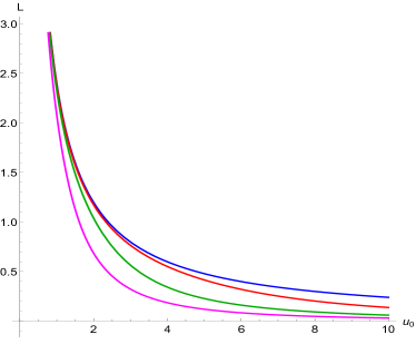
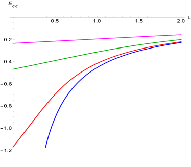
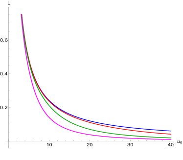
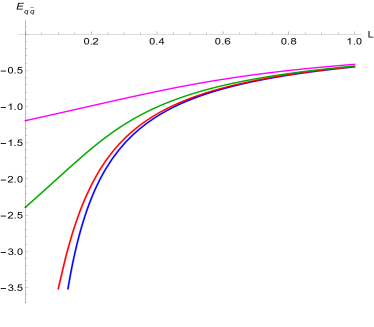
Figure 1: Plots of the length of the WL as a function of the penetration parameter $u_{0}$ (left panels) and of the energy of the WL as a function of the length (right panels) for two different values of the deformation parameter $\tilde{\gamma}$. More specifically, the upper two plots are for $\tilde{\gamma}=0$ and the lower two plots are for $\tilde{\gamma}=5$. The angle between the quarks along the five sphere is kept fixed at the value $\Delta\chi={\pi\over 16}\sqrt{1+\tilde{\gamma}^{2}}$ . Different colors correspond to different values of the deformation parameter $\tilde{\mu}$: blue for $\tilde{\mu}=0$, red for $\tilde{\mu}=0.2$, green for $\tilde{\mu}=0.5$ and magenta for $\tilde{\mu}=1$

Fitting the data of the plots from figure 1 in the region where $u_{0}$ is small, we see that for both values of the deformation parameter $\tilde{\gamma}$ and for all the values of the deformation parameter $\tilde{\mu}$, the length is inverse proportional to $u_{0}$ and the energy is inverse proportional to the length. Based on that observation we conclude that for large values of $\mathbb{L}$, when the Wilson loop is probing the far interior of the background and the quarks are far away from each other, the geometry has $AdS$ characteristics.

This picture changes considerably when the value of $u_{0}$ increases. This can be seen explicitly, since the elliptic integrals in equations (68), (69) and (72) can be expanded perturbatively. To simplify the analytic expressions, the constant value of the angle is denoted as

$$\Delta\chi=\ell\,\pi\,\sqrt{1+\tilde{\gamma}^{2}}$$ (73)

where $\ell$ is a constant. Inspired by the fitting of the numerical data that we have already obtained, we introduce the following ansatz for $\kappa$ in (69)

$$2\,\kappa\,\tilde{\mu}=1-\frac{1+\tilde{\gamma}^{2}}{4}\,\frac{1}{\tilde{\mu}^{2}u_{0}^{2}}-\frac{\left(1+\tilde{\gamma}^{2}\right)^{2}}{8}\,\frac{1-2\,\ell}{\tilde{\mu}^{4}u_{0}^{4}}-\frac{\left(1+\tilde{\gamma}^{2}\right)^{3}}{64}\,\frac{3-28\,\ell+30\,\ell^{2}}{\tilde{\mu}^{6}u_{0}^{6}}$$ (74)

and expanding in large values of $u_{0}$ we determine the coefficients. Substituting (74) in (68) and (72) we obtain the following expressions for the length

$$\mathbb{L}=\frac{\pi}{\tilde{\mu}\,u_{0}^{2}}\sqrt{\big{.}\left(1+\tilde{\gamma}^{2}\right)(1-\ell)}\Bigg{[}1-\frac{1+\tilde{\gamma}^{2}}{16}\,\frac{\ell+7}{\tilde{\mu}^{2}u_{0}^{2}}+\frac{\left(1+\tilde{\gamma}^{2}\right)^{2}}{512}\,\frac{99-26\,\ell+135\,\ell^{2}}{\tilde{\mu}^{4}u_{0}^{4}}\Bigg{]}$$ (75)

and for the energy

$$E_{q\bar{q}}=-\frac{1-\ell}{4\,\tilde{\mu}}\sqrt{1+\tilde{\gamma}^{2}}\Bigg{[}1-\frac{1+\tilde{\gamma}^{2}}{2\,\tilde{\mu}^{2}\,u_{0}^{2}}+\frac{\left(1+\tilde{\gamma}^{2}\right)^{2}}{64}\,\frac{11+17\ell}{\tilde{\mu}^{4}\,u_{0}^{4}}\Bigg{]}$$ (76)

as expansions in inverse powers of $u_{0}$. Combining (75) and (76) we obtain the following expression for the energy in powers of the length

$$E_{q\bar{q}}=-\frac{1-\ell}{4\,\tilde{\mu}}\sqrt{1+\tilde{\gamma}^{2}}+\frac{(1+\tilde{\gamma}^{2})\sqrt{1-\ell}}{8\,\pi\,\tilde{\mu}^{2}}\,\mathbb{L}+\frac{3\left(1+\tilde{\gamma}^{2}\right)^{3\over 2}\,\left(1-5\,\ell\right)}{256\,\pi^{2}\,\tilde{\mu}^{3}}\,\mathbb{L}^{2}\cdots\,.$$ (77)

In figure 2 we compare the perturbative expansions of the length and of the energy with respect to the numerical counterparts. Keeping the same number of terms in the expansion, the overlap of the two curves (numerical and perturbative) is maintained for larger values of the length, the lower the value of the deformation parameter $\tilde{\mu}$ is.

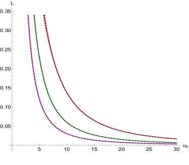
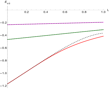
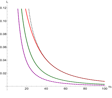
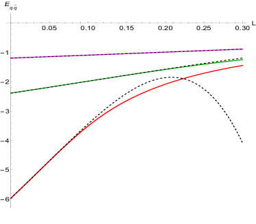
Figure 2: Zooming in of the plots of figure 1 in the region of large values of $u_{0}$ or equivalently of small values of $\mathbb{L}$. The solid lines are the result of the numerical evaluation, while for the dotted black lines we have used the perturbative expressions, namely equations (75) and (77).

There are various interesting conclusions to draw from the preceding analysis and especially from equation (77). As immediate observation is that as the length of the Wilson loop decreases, the energy instead of decreasing to minus infinity which would be the expected $AdS$ behavior, flows to a finite value that is inversely proportional to the deformation parameter $\tilde{\mu}$. As a result, by increasing the value of $\tilde{\mu}$ we can bring the quarks close to each other with less energy cost and in the limit of $\tilde{\mu}\rightarrow\infty$ we have complete screening. Another striking feature of (77) is that for small values of the boundary distance the energy is linear in the length and a confining behavior arises. This behavior remains dominant for the Wilson loop until an inflection point in the plot of the energy versus the length is reached. This is not easily seen by looking in the plots of figure 1 and one has to draw the first and the second derivative of the energy with respect to the length. It is after that point that the characteristic $AdS$ structure that we described previously emerges. In figure 3 we have plotted the length and the energy of the inflection point as functions of the deformation parameter $\tilde{\mu}$. The length is almost linear in $\tilde{\mu}$ while the energy is inverse proportional. Notice that the inflection point we calculate numerically is different from the inflection point that one could calculate using the perturbative expansion for the energy in (77). This is not surprising since as can be seen from figure 3, for large enough values of $\tilde{\mu}$ the inflection point is not anymore close to the $\mathbb{L}\rightarrow 0$ limit.

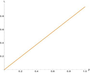
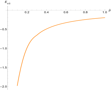
Figure 3: Plots of the length (left panel) and of the energy (right panel) of the inflection point as functions of the deformation parameter $\tilde{\mu}$. When the length is smaller, the Wilson loop has a confining behavior. Fitting the data we confirm that the length is linear in $\tilde{\mu}$ while the energy is inverse proportional.

The analysis of the behavior of the Wilson loop is telling us that in order to probe the effect of the deformation parameter $\tilde{\mu}$ in the geometry, we have to stay close to the boundary (where $u_{0}$ is large and consequently $\mathbb{L}$ is small) and not penetrate deep in the IR. This is explained by the fact that in the reduced metric (59) the term that contains the effect of the $\tilde{\mu}$ becomes important when $u$ is large, i.e. close to the boundary. This is a behavior that distinguishes the Schrödinger solution from all the other TsT transformed backgrounds.

6 Giant Graviton

In this section we will present the Giant Graviton solution in the background that was constructed in section 2. The bottom-line of the computation is that despite the presence of both the Schrödinger and the marginal parameters (namely $\mu$ and $\gamma$) in the background, the energy of the Giant Graviton depends only on $\mu$. The parameter $\gamma$ disappears from the computation. As a result, the analysis of the Giant Graviton’s energy reduces to the discussion that was presented in Georgiou:2020wwo . Here we will examine the technicalities behind the $\gamma$ cancellation. Notice the following: in the literature it is known that in the marginally deformed backgrounds the energy of the Giant Graviton is blind to the presence of the $\gamma$ deformation (see for example Pirrone:2006iq ; Pirrone:2008av ; Imeroni:2006rb ). However, since in the background of section 2 there is a mixing between the two deformations, a term with a $\gamma$ dependence could potentially survive. In the following we will see why this is not the case.

To proceed with the computation along the lines of Grisaru:2000zn , we perform the following change of variables in (2)

$$\rho=\sin\eta\,.$$ (78)

To construct the WZ term of the D3-brane action that describes the Giant Graviton, we need to determine the RR potentials. For $F_{3}$ in (6) we determine $C_{2}$ as follows

$$F_{3}=dC_{2}\quad\Rightarrow\quad\frac{C_{2}}{R^{2}}\,=\,-\,\frac{1}{8}\,\gamma\,\rho^{4}\,\sin\theta\,d\rho\wedge d\theta\wedge d\phi$$ (79)

while from the definition for $F_{5}$

$$F_{5}=dC_{4}-H_{3}\wedge C_{2}$$ (80)

and (6), we obtain an expression for $C_{4}$ that has a smooth zero deformation limit

$$\frac{C_{4}}{R^{4}}=-\,\frac{1}{z^{4}}\,dt\wedge dv\wedge dx_{1}\wedge dx_{2}+\frac{\rho^{4}}{8}\sin\theta\,d\theta\wedge d\phi\wedge d\chi\wedge d\psi+B_{2}\wedge C_{2}\,.$$ (81)

Now that all the potentials are known, we have to consider the action of a probe D3-brane to describe Giant Graviton solutions in (2). The action has the usual form

$$S_{{\rm D}3}=-T_{3}\int d^{4}\xi\,e^{-\Phi}\sqrt{\big{.}-\det{\cal P}\Big{[}g-B+2\pi\alpha^{\prime}F\Big{]}}+T_{3}\int\sum_{q}{\cal P}\Big{[}C_{q}\wedge e^{-B+2\pi\alpha^{\prime}F}\Big{]}$$ (82)

where ${\cal P}$ denotes the pullback on the brane worldvolume directions and $T_{3}$ is the tension of the D3-brane. An important comment is in order: Notice that expanding the exponential of the WZ term, the combination of the potentials that will contribute to the action is $C_{4}-B_{2}\wedge C_{2}$. From (81) we observe that this combination is deformation independent. This means that the WZ contribution to the action will be identical to the undeformed case and all the potential deformation dependence will come only from the DBI term. To see whether this happens, we have to consider a consistent ansatz for the D3-brane embedding. The D3-brane probe we consider extends along the following directions

$$\xi_{0}=\tau\,,\quad\xi_{1}=\theta\,,\quad\xi_{2}=\phi\quad\&\quad\xi_{3}=\psi$$ (83)

while the ansatz for the embedding is the following

$$t=\,\frac{\tau}{R}\,,\quad v=\nu\,\tau\,,\quad\vec{x}=0\,,\quad z=z_{0}\,,\quad\rho=\frac{\rho_{0}}{R}\quad\&\quad\chi=\omega\,\tau$$ (84)

with $\rho_{0}$ being the size of the graviton in the internal space.

Substituting the ansatz (84) in the D3-brane action (82) and integrating, an impressive cancellation occurs and, we obtain the on-shell action and the Lagrangian of Georgiou:2020wwo that only depend on the Schrödinger deformation parameter $\mu$. The presence of the dilaton in the string frame DBI term is essential for the $\gamma$ cancelation in the action. The Lagrangian becomes

$$L_{{\rm D}3}=-\,\frac{N}{R^{4}}\,\Bigg{[}\rho_{0}^{3}\,\sqrt{1-\Gamma-\left(R^{2}-\rho_{0}^{2}\right)\,\left(\omega^{2}-\frac{\Delta^{2}}{R^{2}}\right)}-\rho_{0}^{4}\,\omega\Bigg{]}$$ (85)

where the different constants are defined as follows

$$\kappa=\frac{1}{R}\ ,\quad\Gamma=\frac{2\,R}{Z_{0}^{2}}\,\nu\ ,\quad\Delta=\frac{\mu}{Z_{0}^{2}}\quad\&\quad 2\,\pi^{2}\,T_{3}=\frac{N}{R^{4}}\,.$$ (86)

From this point on the analysis is identical to the case that only the Schrödinger deformation is present and can be found in Georgiou:2020wwo . Notice that if one performs a stability analysis around the Giant Graviton solution in (84), the vibration modes will depend on both deformation parameters $\mu$ and $\gamma$. Support on this argument is coming from the study of the spectra of frequencies (for both the scalar and the gauge fields) in the $\gamma$ deformed backgrounds Pirrone:2006iq ; Pirrone:2008av ; Avramis:2007wb .

7 PP-wave background and the string spectrum

In this section we consider the Penrose limit of the deformed solution that was constructed in section 2, around a geodesic that sits at $\eta=0$. Notice that this geodesic and the corresponding dispersion relation do not depend on the deformation parameter $\gamma$. In order to have a geodesic with such a dependence, we have to set the value of $\eta$ different from $0$. If we set $\eta=\pi/2$, which is the case we analyzed in section 4, then we have a degenerate solution since the determinant of the metric of the pp-wave background is zero. This fact implies that we lose one of the coordinates and the pp-wave backround becomes 9-dimensional, a feature that is undesirable. On the other hand, if we keep the value of $\eta$ fixed but arbitrary, then in order for the geodesic ansatz to be consistent we have to fix the value of $\omega$ in terms of the deformation parameters. In this way we obtain a pp-wave solution, but with the cost that it is extremely complicated, e.g. it is impossible to bring it in the Brinkmann form and study the spectrum of bosonic excitations. For all these reasons we choose to expand around $\eta=0$.

In particular, we expand the coordinates in the following way

$$t=\kappa\,U\,,\quad v=\mu^{2}\,m\,U-\frac{\omega}{m}\,\frac{y_{2}}{R}\,,\quad\chi=\omega\,U+\frac{y_{2}}{R}+\frac{1}{\omega}\,\frac{V}{R^{2}}\,,$$ (87)

$$z=\sqrt{\frac{\kappa}{m}}\,\Big{(}1+\frac{y_{1}}{R}\Big{)}\,,\quad x_{1}=\sqrt{\frac{\kappa}{m}}\,\frac{y_{3}}{R}\,,\quad x_{2}=\sqrt{\frac{\kappa}{m}}\,\frac{y_{4}}{R}\quad\&\quad\eta=\frac{r}{R}\,.$$

One can check that the dominant terms of the previous expansion in the $R\rightarrow\infty$ limit guarantee that the null condition for the geodesic is satisfied, provided that the parameters $\kappa$, $\omega$ and $m$ are related through the following dispersion relation

$$\kappa^{2}=\omega^{2}+m^{2}\mu^{2}\,.$$ (88)

Notice that although this dispersion relation is $\gamma$ independent the spectrum of the pp-wave background will depend on $\gamma$ in a non-trivial way.

Using the aforementioned expansion for the coordinates and taking the limit $R\rightarrow\infty$ in the line element, we end up with the following expression

$$ds^{2}_{pp}=2\,dU\,dV+\Bigg{[}2\,\omega\Big{(}y_{1}\,dy_{2}-y_{2}\,dy_{1}+y_{5}\,dy_{6}-y_{6}\,dy_{5}+y_{7}\,dy_{8}-y_{8}\,dy_{7}\Big{)}$$ (89)

$$\qquad+\mu\,m\,\gamma\,\Big{(}y_{6}\,dy_{5}-y_{5}\,dy_{6}+y_{7}\,dy_{8}-y_{8}\,dy_{7}\Big{)}\Bigg{]}dU+\sum\limits_{i=1}^{8}dy^{2}_{i}-F\,dU^{2}\,,$$

$${\rm where}\quad F=4\,\mu^{2}\,m^{2}\,y^{2}_{1}+\big{(}\mu^{2}\,m^{2}+\omega^{2}\big{)}\big{(}y^{2}_{3}+y^{3}_{4}\big{)}-\frac{\gamma^{2}}{4}\,\big{(}\mu^{2}\,m^{2}-\omega^{2}\big{)}\sum\limits_{i=5}^{8}y^{2}_{i}\,.$$

Moreover, in order to arrive to the previous expression for the metric of the pp-wave we considered the following change of coordinates

$$y_{5}+i\,y_{6}\,=\,r\,\sin\frac{\theta}{2}\,e^{i\frac{\phi+\psi}{2}}\quad\&\quad y_{8}+i\,y_{7}\,=\,r\,\cos\frac{\theta}{2}\,e^{i\frac{\phi-\psi}{2}}$$ (90)

and shifted $V$ as follows: $V\rightarrow V-\omega\,y_{1}\,y_{2}$. The geometry (89) has a vanishing Ricci scalar (i.e. $R_{\mu}^{\,\,\,\mu}=0)$, as it should be for a pp-wave geometry.

We would like to further simplify the expression for the line element of our pp-wave background and bring it into the Brinkmann form. In order to do this we perform three rotations in the three complex planes defined by the coordinate pairs $(y_{1},y_{2})$, $(y_{5},y_{6})$ and $(y_{7},y_{8})$ as it is described in the following relations

$$y_{1}+i\,y_{2}\,=\,\left(\tilde{y}_{1}+i\,\tilde{y}_{2}\right)\,e^{-i\,\omega\,U}\,,\quad y_{5}+i\,y_{6}\,=\,\left(\tilde{y}_{5}+i\,\tilde{y}_{6}\right)\,e^{i\,\frac{\mu\,m\,\gamma-2\,\omega}{2}\,U}\,,$$ (91)

$$\qquad\qquad\qquad y_{8}+i\,y_{7}\,=\,\left(\tilde{y}_{8}+i\,\tilde{y}_{7}\right)\,e^{i\,\frac{\mu\,m\,\gamma+2\,\omega}{2}\,U}\,.$$

After dropping the tildes, the geometry has the standard line element

$$ds^{2}_{pp}\,=\,2\,dU\,dV+\sum\limits_{i=1}^{8}dy^{2}_{i}-H\,dU^{2}$$ (92)

and the function $H$ is defined as follows

$$H = \omega^{2}\big{(}y^{2}_{1}+y^{2}_{2}\big{)}+\big{(}\mu^{2}\,m^{2}+\omega^{2}\big{)}\big{(}y^{2}_{3}+y^{2}_{4}\big{)}+\frac{\omega}{4}\Big{[}\big{(}4+\gamma^{2}\big{)}\,\omega-4\,\mu\,m\,\gamma\Big{]}\big{(}y^{2}_{5}+y^{2}_{6}\big{)}$$ (93)

$$+ \frac{\omega}{4}\Big{[}\big{(}4+\gamma^{2}\big{)}\,\omega+4\,\mu\,m\,\gamma\Big{)}\big{(}y^{2}_{7}+y^{2}_{8}\big{)}+4\,\mu^{2}\,m^{2}\Big{[}y_{1}\,\cos(\omega\,U)+y_{2}\,\sin(\omega\,U)\Big{]}^{2}\,.$$

The geometry is supported by a NS $2-$form and a RR $5-$form

$$B_{2} =\mu\,m\,dU\wedge\Big{(}y_{2}\,dy_{1}-y_{1}\,dy_{2}+y_{5}\,dy_{6}-y_{6}\,dy_{5}+y_{7}\,dy_{8}-y_{8}\,dy_{7}\Big{)}$$ (94)

$$+\frac{\gamma\,\omega}{2}dU\wedge\Big{(}y_{6}\,dy_{5}-y_{5}\,dy_{6}+y_{7}\,dy_{8}-y_{8}\,dy_{7}\Big{)}\,,$$

$$F_{5} =4\,\omega\,dU\wedge\Big{(}dy_{1}\wedge dy_{2}\wedge dy_{3}\wedge dy_{4}-dy_{5}\wedge dy_{6}\wedge dy_{7}\wedge dy_{8}\Big{)}\,,$$

where in the expression for the $2-$form we have dropped terms that are total derivatives. Notice that if we set $\gamma=0$ the expressions (92), (93) and (94) reduce to the expressions of Georgiou:2019lqh . Moreover if we set $\mu=0$, we obtain the pp-wave solution that was analyzed in Niarchos:2002fc ; Lunin:2005jy (see also Avramis:2007wb ).

To calculate the spectrum of closed strings propagating on the pp-wave background that is given (92) and (94), we have to write down the bosonic string action and derive the equations of motion. To set-up the conventions, in appendix B we have collected, the Polyakov action and the Virasoro constrains.

Choosing the light-cone gauge (i.e. $U=\alpha^{\prime}p_{+}\tau$), the Virasoro constraints will determine $V$ in terms of the remaining eight degrees of freedom. It turns out that the equations of motion for the scalars $y_{3}$ and $y_{4}$ are completely decoupled, while the rest couple in pairs. Below we analyze them separately.

Equations of motion for $y_{1}\,\&\,y_{2}$

The equations of motion for the scalars $y_{1}$ and $y_{2}$ have a more complicated form due to the explicit dependence on $\tau$

$$\Box\,y_{1}+2\,\alpha^{\prime}\,p_{+}\,\mu\,m\,\partial_{\sigma}y_{2}$$ (95)

$$-\alpha^{\prime 2}\,p_{+}^{2}\Bigg{[}\omega^{2}y_{1}-4\,\mu^{2}m^{2}\cos\big{(}\alpha^{\prime}p_{+}\omega\tau\big{)}\,\Big{[}y_{1}\cos\big{(}\alpha^{\prime}p_{+}\omega\tau\big{)}+y_{2}\sin\big{(}\alpha^{\prime}p_{+}\omega\tau\big{)}\Big{]}\Bigg{]}=0\,,$$

$$\Box\,y_{2}-2\,\alpha^{\prime}\,p_{+}\,\mu\,m\,\partial_{\sigma}y_{1}$$

$$-\alpha^{\prime 2}\,p_{+}^{2}\Bigg{[}\omega^{2}y_{2}-4\,\mu^{2}m^{2}\sin\big{(}\alpha^{\prime}p_{+}\omega\tau\big{)}\,\Big{[}y_{1}\cos\big{(}\alpha^{\prime}p_{+}\omega\tau\big{)}+y_{2}\sin\big{(}\alpha^{\prime}p_{+}\omega\tau\big{)}\Big{]}\Big{]}=0\,.$$

Notice here that this set of equations does not depend on the $\gamma$ deformation parameter and the analysis has been presented in Georgiou:2019lqh . However, in order to be complete we briefly repeat it here. To eliminate the dependence in $\tau$, we perform the following rotation

$$y_{1}=\tilde{y}_{1}\cos\big{(}\alpha^{\prime}p_{+}\omega\tau\big{)}-\tilde{y}_{2}\sin\big{(}\alpha^{\prime}p_{+}\omega\tau\big{)}\,,\quad y_{2}=\tilde{y}_{1}\sin\big{(}\alpha^{\prime}p_{+}\omega\tau\big{)}+\tilde{y}_{2}\cos\big{(}\alpha^{\prime}p_{+}\omega\tau\big{)}\,.$$ (96)

an the system of equations in (95) becomes

$$\Box\,\tilde{y}_{1}-4\,\alpha^{\prime 2}\,p_{+}^{2}\,\mu^{2}\,m^{2}\,\tilde{y}_{1}+2\,\alpha^{\prime}\,p_{+}\big{(}\omega\,\partial_{\tau}\tilde{y}_{2}+\mu\,m\,\partial_{\sigma}\tilde{y}_{2}\big{)}\,=\,0\,,$$ (97)

$$\Box\,\tilde{y}_{2}-2\,\alpha^{\prime}\,p_{+}\big{(}\omega\,\partial_{\tau}\tilde{y}_{1}+\mu\,m\,\partial_{\sigma}\tilde{y}_{1}\big{)}\,=\,0\,.$$

Imposing the ansatz

$$\tilde{y}_{1}=\sum\limits_{n=-\infty}^{\infty}\alpha_{n}e^{-i\tilde{\omega}_{n}\tau+n\sigma}\,,\qquad\tilde{y}_{2}=\sum\limits_{n=-\infty}^{\infty}\beta_{n}e^{-i\tilde{\omega}_{n}\tau+n\sigma}\,,$$ (98)

with $\alpha_{n}$ and $\beta_{n}$ being constants, we end up with a homogeneous algebraic system for $\alpha_{n}$ and $\beta_{n}$. Requiring that the determinant of the matrix that defines the aforementioned algebraic system with respect to $\alpha_{n}$ and $\beta_{n}$ vanishes, we obtain a quartic equation for the eigenfrequencies $\tilde{\omega}_{n}$

$$\tilde{\omega}^{4}_{n}+\gamma_{2}\,\tilde{\omega}^{2}_{n}+\gamma_{1}\,\tilde{\omega}_{n}+\gamma_{0}=0\,,$$ (99)

with

$$\gamma_{0}=n^{4}\,,\quad\gamma_{1}=8\,\alpha^{\prime 2}\,p_{+}^{2}\,\mu\,m\,\omega\,n\quad\&\quad\gamma_{2}=-2\,n^{2}-4\,\alpha^{\prime 2}\,p_{+}^{2}\big{(}\omega^{2}+\mu^{2}\,m^{2}\big{)}\,.$$ (100)

The solution of the quartic equation above is

$$\tilde{\omega}_{n}^{(1)}=-S\pm\frac{1}{2}\sqrt{-4S^{2}-2\gamma_{2}+\frac{\gamma_{1}}{S}}\,,\qquad\tilde{\omega}_{n}^{(2)}=S\pm\frac{1}{2}\sqrt{-4S^{2}-2\gamma_{2}-\frac{\gamma_{1}}{S}}\,,$$ (101)

where

$$S=\frac{1}{2}\sqrt{-\frac{2}{3}\gamma_{2}+\frac{1}{3}\Big{(}Q+\frac{\Delta_{1}}{Q}\Big{)}}\,,\qquad Q^{3}=\frac{1}{2}\Big{(}\Delta_{1}+\sqrt{\Delta_{1}^{2}-4\Delta_{0}^{3}}\Big{)}\,,$$ (102)

$${\rm with}\quad\Delta_{1}=2\,\gamma_{2}^{3}+27\,\gamma_{1}^{2}-72\,\gamma_{2}\,\gamma_{0}\quad\&\quad\Delta_{0}=\gamma_{2}^{2}+12\,\gamma_{0}\,.$$

Equations of motion for $y_{3}\,\&\,y_{4}$

The decoupled equations for the scalars $y_{3}$ and $y_{4}$ do not depend on the $\gamma$ deformation parameter and read

$$\Box y_{i}-\alpha^{\prime 2}p_{+}^{2}\,\kappa^{2}y_{i}=0\,,\qquad i=3,4\,.$$ (103)

These can be easily solved using the plane wave ansatz $y_{i}\sim e^{-i\,\omega_{i;n}\,\tau+i\,n\,\sigma}$ which implies that the eigenfrequencies for $y_{i}$ are

$$\omega^{2}_{i;n}=\alpha^{\prime 2}\,p_{+}^{2}\,\kappa^{2}+n^{2}=\alpha^{\prime 2}\,p_{+}^{2}\,\big{(}\omega^{2}+\mu^{2}\,m^{2}\big{)}+n^{2}\,,\qquad i=3,4\,.$$ (104)

Equations of motion for $y_{5}\,\&\,y_{6}$

We now move to the equations for the scalars $y_{5}$ and $y_{6}$, which are coupled due to the derivative terms

$$\Box\,y_{5}-\alpha^{\prime 2}\,p_{+}^{2}\,\omega\left[\left(1+\frac{\gamma^{2}}{4}\right)\omega-\mu\,m\,\gamma\right]y_{5}+\alpha^{\prime}\,p_{+}\big{(}\gamma\,\omega-2\,\mu\,m\big{)}\partial_{\sigma}y_{6}=0\,,$$ (105)

$$\Box\,y_{6}-\alpha^{\prime 2}\,p_{+}^{2}\,\omega\left[\left(1+\frac{\gamma^{2}}{4}\right)\omega-\mu\,m\,\gamma\right]y_{6}-\alpha^{\prime}\,p_{+}\big{(}\gamma\,\omega-2\,\mu\,m\big{)}\partial_{\sigma}y_{5}=0\,.$$

The above set of equations can be decoupled if we consider the linear combinations $y^{\pm}_{56}=y_{5}\pm iy_{6}$. Then for the $y^{\pm}_{56}$ we get

$$\Box y^{+}_{56}-\alpha^{\prime 2}p_{+}^{2}\omega\left[\left(1+\frac{\gamma^{2}}{4}\right)\omega-\mu\,m\,\gamma\right]y^{+}_{56}-i\,\alpha^{\prime}\,p_{+}\big{(}\gamma\,\omega-2\,\mu\,m\big{)}\partial_{\sigma}y^{+}_{56}=0\,,$$ (106)

$$\Box y^{-}_{56}-\alpha^{\prime 2}p_{+}^{2}\omega\left[\left(1+\frac{\gamma^{2}}{4}\right)\omega-\mu\,m\,\gamma\right]y^{-}_{56}+i\,\alpha^{\prime}\,p_{+}\big{(}\gamma\,\omega-2\,\mu\,m\big{)}\partial_{\sigma}y^{-}_{56}=0\,.$$

Choosing again a plane-wave ansatz $y^{\pm}_{56}\sim e^{-i\omega^{\pm}_{56;n}\tau+in\sigma}$ we get

$$\big{(}\omega^{\pm}_{56;n}\big{)}^{2}=\alpha^{\prime 2}\,p_{+}^{2}\,\omega\left[\left(1+\frac{\gamma^{2}}{4}\right)\omega-\mu\,m\,\gamma\right]\pm n\,\alpha^{\prime}\,p_{+}\big{(}2\,\mu\,m-\gamma\,\omega\big{)}+n^{2}\,.$$ (107)

It is important to notice that the frequencies depend on both deformation parameters $\mu$ and $\gamma$ in a non-trivial way.

Equations of motion for $y_{7}\,\&\,y_{8}$

The equations for the scalars $y_{7}$ and $y_{8}$ can be treated similarly to those for $y_{5}$ and $y_{6}$. In particular we have that

$$\Box\,y_{7}-\alpha^{\prime 2}\,p_{+}^{2}\,\omega\left[\left(1+\frac{\gamma^{2}}{4}\right)\omega+\mu\,m\,\gamma\right]y_{7}-\alpha^{\prime}\,p_{+}\big{(}\gamma\,\omega+2\,\mu\,m\big{)}\partial_{\sigma}y_{8}=0\,,$$ (108)

$$\Box\,y_{8}-\alpha^{\prime 2}\,p_{+}^{2}\,\omega\left[\left(1+\frac{\gamma^{2}}{4}\right)\omega+\mu\,m\,\gamma\right]y_{8}+\alpha^{\prime}\,p_{+}\big{(}\gamma\,\omega+2\,\mu\,m\big{)}\partial_{\sigma}y_{7}=0\,.$$

Notice that these can be obtained from the equations of motion for $y_{5}$ and $y_{6}$ in (105) by sending $y_{5}\mapsto y_{8}$, $y_{6}\mapsto y_{7}$ and $\mu\mapsto-\mu$. Thus the eigenfrequencies for the decoupled scalars $y^{\pm}_{78}=y_{8}\pm iy_{7}$ can be obtained from those for $y^{\pm}_{56}$ in eq. (107) simply by sending $\mu\mapsto-\mu$, i.e.

$$\big{(}\omega^{\pm}_{78;n}\big{)}^{2}=\alpha^{\prime 2}\,p_{+}^{2}\,\omega\left[\left(1+\frac{\gamma^{2}}{4}\right)\omega+\mu\,m\,\gamma\right]\mp n\,\alpha^{\prime}\,p_{+}\big{(}2\,\mu\,m+\gamma\,\omega\big{)}+n^{2}\,.$$ (109)

Notice that in the case of $\gamma=0$ we obtain the frequencies of the Schrödinger background that were computed in Georgiou:2019lqh , while for $\mu=0$ the frequencies in (101), (104), (107) and (109) reduce to those computed in Niarchos:2002fc ; Lunin:2005jy (see also Avramis:2007wb ).

Moreover, in the pp-wave background, one can try to construct a Giant Graviton solution in the same way that we did in section 6. The bottomline of the construction is that this pp-wave graviton, in the same way as the graviton of section 6, will be independent of the $\gamma$ deformation parameter. As a result such a computation reduces to the computation of Georgiou:2020qnh . In order to obtain a Giant Graviton that depends on the $\gamma$ deformation parameter, one should try for a different geodesic.

7.1 PP-wave spectrum and dispersion of the giant magnon

In this section, and based on the bosonic spectrum on the pp-wave background derived in the previous section, we make an educated guess for the exact in $\lambda$ anomalous dimensions of the operators that are dual to the string excitations (104), (107) and (109). To this end we closely follow section 4 of Georgiou:2019lqh .

One starts from the fact that the light-cone string Hamiltonian is linear in the generators $E$, $M$ and $J$, namely,

$$H_{\rm l.c.}\equiv p^{-}=p_{+}=i\frac{\partial}{\partial x^{+}}=i\Bigg{[}\kappa{\partial\over\partial T}+\omega{\partial\over\partial\chi}+\mu^{2}m{\partial\over\partial V}\Bigg{]}\,.$$ (110)

Furthermore, since the conserved charges in the original Schrödinger background are given by

$$E=i\,{\partial\over\partial T}\,,\quad J=-\,i\,{\partial\over\partial\chi}\ ,\quad M\,=\,-\,i\,{\partial\over\partial V}\,,$$ (111)

one gets the following relation for the light-cone Hamiltonian in terms of the conserved charges of the original doubly deformed spacetime

$$H_{\rm l.c.}=\kappa E-\omega J-\mu^{2}mM\,.$$ (112)

Additionally, the light-cone momentum is given by

$$\alpha^{\prime}p^{+}=\alpha^{\prime}p_{-}=-i\alpha^{\prime}\frac{\partial}{\partial x^{-}}=-i{\alpha^{\prime}\over\omega R^{2}}{\partial\over\partial\chi}={J\over\sqrt{\lambda}}\,.$$ (113)

In (113), in order to simplify the notation, we have set $\omega=1$ and we have also used the relation between the radius $R$ and the ’t Hooft coupling $\lambda$, that is $R^{2}/\alpha^{\prime}=\sqrt{\lambda}$.

By identifying the light-cone Hamiltonian (112) with the energy of a single string excitation given by (109), that is $H_{\rm l.c.}=\omega^{\pm}_{78;n}$, one gets that

$${\kappa\,\sqrt{\lambda}E-\mu^{2}m\sqrt{\lambda}M\over J}-\sqrt{\lambda}=\sqrt{1+{\gamma^{2}\over 4}+\mu m\gamma+{n^{2}\lambda\over J^{2}}\mp{n(2\mu m+\gamma)\sqrt{\lambda}\over J}}\ .$$ (114)

The next step is to write the angular momentum, energy and particle number of the string moving on the pp-wave geometry as the corresponding quantities of the point-like BMN particle plus corrections of order $\mathcal{O}(\lambda^{0})$, that is

$$E=\sqrt{\lambda}\kappa+\epsilon_{1}\ ,\quad J=\sqrt{\lambda}+j_{1}\ ,\quad M=\sqrt{\lambda}m+m_{1}\ .$$ (115)

One then solves (115) for the quantities $\sqrt{\lambda}\kappa$, $\sqrt{\lambda}$ and $\sqrt{\lambda}m$ in terms of $E$, $J$ and $M$ and substitute the resulting expressions in (114) to obtain

$${E^{2}-\mu^{2}M^{2}\over J}-J-Y_{1}=\sqrt{1+{\gamma^{2}\over 4}+\mu m\gamma+{n^{2}\lambda\over J^{2}}\mp{n(2\mu m+\gamma)\sqrt{\lambda}\over J}}\ ,$$ (116)

where $Y_{1}$ collects the terms involving $\epsilon_{1},j_{1}$ and $m_{1}$ and is given by

$$Y_{1}={\epsilon_{1}E-\mu^{2}Mm_{1}\over J}-j_{1}\,.$$ (117)

The last step is to express $J$ in terms of $E$, $\epsilon_{1}$, $M$, $m_{1}$ and $j_{1}$. This can be done by plugging (115) in the holding relation $\kappa^{2}=\mu^{2}m^{2}+\omega^{2}$ to get

$$E^{2}-\mu^{2}M^{2}-J^{2}=Z\quad{\rm with}$$ (118)

$$Z=2\left(\epsilon_{1}\kappa\sqrt{\lambda}-\sqrt{\lambda}j_{1}-\mu^{2}m\sqrt{\lambda}m_{1}\right)+\epsilon_{1}^{2}-j_{1}^{2}-\mu^{2}m_{1}^{2}\ .$$

The first equation in (118) can now be solved for $J$ to give

$$J=\sqrt{E^{2}-\mu^{2}M^{2}}\Bigg{[}1-{1\over 2}{Z\over E^{2}-\mu^{2}M^{2}}\Bigg{]}\,,$$ (119)

where in order to derive this last equation we have approximated $\sqrt{1-{Z\over E^{2}-\mu^{2}M^{2}}}$ by $1-{1\over 2}{Z\over E^{2}-\mu^{2}M^{2}}$, since $Z$ is of ${\cal O}(\sqrt{\lambda})$ while $E^{2}-\mu^{2}M^{2}$ is of ${\cal O}(\lambda)$.

The result for $J$ should be now substituted in (116) to give

$$\sqrt{E^{2}-\mu^{2}M^{2}}-J=\sqrt{1+{\gamma^{2}\over 4}+\mu m\gamma+{n^{2}\lambda\over J^{2}}\mp{n(2\mu m+\gamma)\sqrt{\lambda}\over J}}+{\cal W}\ ,$$ (120)

with

$${\cal W}={1\over 2\,J}\,\left(\epsilon_{1}^{2}\,-\,j_{1}^{2}\,-\,\mu^{2}\,m_{1}^{2}\right)\,+\,\frac{Z^{2}}{4\,J\,\left(Z+J^{2}\right)}\,.$$ (121)

Let us stress that ${\cal W}$ in (120) should be ignored since it scales as ${1/J}$ and it becomes zero in the strict $J$ infinity limit in which the giant magnon is defined.

In precisely the same way one obtains the following exact in $\lambda^{\prime}={\lambda\over J^{2}}$ dispersion relation for the excitations of (107).

$$\sqrt{E^{2}-\mu^{2}M^{2}}-J=\sqrt{1+{\gamma^{2}\over 4}-\mu m\gamma+{n^{2}\lambda\over J^{2}}\pm{n(2\mu m-\gamma)\sqrt{\lambda}\over J}}\ .$$ (122)

Finally, for the excitations of (104) which do not depend at all on $\gamma$ one straightforwardly obtains

$$\sqrt{E^{2}-\mu^{2}M^{2}}-J=\sqrt{1+\mu^{2}m^{2}+{n^{2}\lambda\over J^{2}}}\ .$$ (123)

We close this section by making an educated guess for the exact in $\lambda$ dispersion relation of the magnon excitations in the original doubly deformed background. Indeed, inspired by the form of the pp-wave spectrum it is plausible to conjecture that the exact dispersion relation corresponding to (123) is given by

$$\sqrt{E^{2}-\mu^{2}M^{2}}-J=\sqrt{1+\mu^{2}m^{2}+\frac{\lambda}{\pi^{2}}\sin^{2}\frac{p}{2}}\,,\quad J\rightarrow\infty\ ,$$ (124)

while the ones corresponding to (122) and (120) are given by (for $J\rightarrow\infty$)

$$\sqrt{E^{2}-\mu^{2}M^{2}}-J=\sqrt{1+{\gamma^{2}\over 4}-\mu m\gamma+\frac{\lambda}{\pi^{2}}\sin^{2}\frac{p}{2}\pm\left(\mu m-{\gamma\over 2}\right)\frac{\sqrt{\lambda}}{\pi}\,\sin{p}}$$ (125)

and

$$\sqrt{E^{2}-\mu^{2}M^{2}}-J=\sqrt{1+{\gamma^{2}\over 4}+\mu m\gamma+\frac{\lambda}{\pi^{2}}\sin^{2}\frac{p}{2}\mp\left(\mu m+{\gamma\over 2}\right)\frac{\sqrt{\lambda}}{\pi}\,\sin{p}}$$ (126)

respectively.

Indeed, for small values of the momentum $p=\frac{2\pi n}{J},\,\,\,n\in Z$ one gets (123), (122) and (120) respectively. It would be interesting to identify the corresponding field theory operators and check whether their exact in $\lambda$ conformal dimensions are indeed given by (124), (125) and (126). It is important to note that these dispersion relations can be rewritten in a form relevant for the dual null dipole doubly deformed CFT of section 3 by using the relations $\mu=\frac{\sqrt{\lambda}}{2\pi}L$ and $\gamma=\frac{\sqrt{\lambda}}{4\pi}\tilde{\gamma}$ (see Guica:2017mtd ), where $\tilde{L}$ and $\tilde{\gamma}$ are the parameters entering the star product that deforms the parent theory, ${\cal N}=4$ SYM. Having done this, equations (124), (125) and (126) have the correct weak coupling expansion in integer powers of $\lambda$. A final comment is in order. Note that for $\gamma=0$ and $\lambda\gg 1$ the dispersion relations (124), (125) and (126) reduce to the dispersion relation of the giant magnon solution of Georgiou:2017pvi , while for $\mu=0$ and $\lambda\gg 1$ to the dispersion relation of the giant magnon solution of Chu:2006ae .

8 Conclusions

In this work we performed a thorough and detailed study of a new example of the AdS/CFT correspondence, namely of the marginally deformed Schrödinger background. From the gravity side this solution is constructed by performing a series of TsT transformations along two of the five-sphere isometries of the Schrödinger solution. As a result the background depends on two deformation parameters and is integrable for large number of colours $N$. From the field theory side, the Lagrangian of the theory is obtained from that of $\mathcal{N}=4$ SYM by introducing the appropriate star product among the fields. The resulting gauge theory is integrable at the planar level.

Putting an emphasis on the study of the correspondence for this doubly-deformed background, we identified a point-like string solution that depends on both deformation parameters and we derived its dispersion relation. Exploiting the power of the correspondence, we identified the dual field theory operators and using the Landau-Lifshitz coherent state approach, we managed to reproduce the leading terms of the aforementioned dispersion relation. This is a highly non-trivial test of the correspondence. We performed the computation at leading order, in which case the two deformations are disentangled. It would be very interesting to extend this calculation beyond the leading order, that would include terms depending on products of the two deformations simultaneously. In this case the corresponding Hamiltonian wouldn’t be the sum of two terms, one related to $AdS_{3}$ and the other to $S^{3}$, as it happens with the one loop Hamiltonian (32).

Moving forward to the study of field theory observables through their gravity realisation, we focused our attention on the evaluation of the Wilson loop expectation value. The Wilson loop consists of two straight lines extending along the time direction and sitting at two points in space separated by a distance $\mathbb{L}$. We calculate the energy of this configuration as a function of the separation length. This corresponds, as usual, to the potential between two quarks sitting at a distance $\mathbb{L}$ on the boundary Maldacena:1998im . We identified an embedding ansatz for the string that depends on both deformation parameters and calculated the energy of the aforementioned configuration as a function of the separation boundary length. The behaviour of the energy exhibits interesting properties: For values of the length much smaller than the Schrödinger parameter, the energy is inversely proportional to the $\mathbb{L}$, a behaviour that resembles that of a conformal theory. When the separation length is much less than the Schrödinger parameter, an intriguing confining behaviour arises. The energy is linearly proportional to the length with the constant of proportionality being inversely proportional to $\mu^{2}$. As $\mu\to 0$, we obtain the expected conformal behaviour for all the values of the length. Notice here that the observations we detailed above hold for every value of the deformation parameter $\gamma$. Essentially the presence of $\gamma$ is only “dressing” the results, but does not alter their qualitative characteristics or the physical interpretation.

The next observable we shed the light on was the Giant Graviton solution. Even if both deformation parameters appear in the induced metric of the D3-brane action, a cancellation takes place and the marginal deformation $\gamma$ disappears from the energy of the Giant Graviton. It would be very interesting to perform a stability analysis around the aforementioned solution. Based on similar cases in the literature, the vibration modes will depend on both deformation parameters $\mu$ and $\gamma$. Examining those modes a relation between the parameters might arise, in order for the solution to be stable.

It is well-known that string theory is solvable in the pp-wave limit. Furthermore, the spectrum of the strings on the pp-wave background provides information about the dimensions of a particular subsector of gauge theory operators having large charges. Having these in mind we took the Penrose limit of the marginally deformed Schrödinger background along a certain null geodesic. This geodesic was special, in the sense that the final background has a dependence on both deformation parameters. To elaborate on the pp-wave solution we have calculated the spectrum of closed bosonic strings in the deformed background. The eigenfrequencies of the eight transverse physical degrees of freedom give a prediction for the anomalous dimensions of the dual field theory operators as an exact function of the effective coupling $\lambda^{\prime}={\lambda\over J^{2}}$. Four of the eigenfrequencies depend only on the Schrödinger parameter while the remaining four depend on both the marginal and the Schrödinger parameters. Finally, based on the string spectrum on the pp-wave geometry, we made an educated guess for the exact in $\lambda$ dispersion relation of the magnon excitations in the original doubly deformed background which provides us with an exact prediction for the dimensions of the dual field theory operators.

The analysis we performed so far leaves a number of interesting open questions, besides the ones we have already discussed in the process of summarizing our findings. An important calculation that can be done is the construction of the Giant Magnon solution and the corresponding computation of its dispersion relation. With the proper ansatz this relation would depend on both deformation parameters. Notice that while in the present work the dispersion relation on the pp-wave background is exact in $\lambda^{\prime}$ with the momentum of the magnon being $p\ll 1$, the dispersion relation of the Giant Magnon will be in the strong coupling regime $\lambda\gg 1$ with the momentum excitation being finite. While the two computations are independent and different, there is a region of the parametric space for which there is an overlap. In section 7.1, we made an informed guess for the exact in $\lambda$ dispersion relation of the giant magnon in the background (2), (4) and (5). It would be interesting to identify the exact form of the field theory operators and calculate their anomalous dimension in order to test these dispersion relations at the weak coupling regime. Along the same lines, one may try to employ, after generalising, the method of Guica:2017mtd that is based on the Q-Baxter equation in order to calculate the spectrum of our doubly deformed background. This is necessary since, like in Guica:2017mtd , the corresponding to (9) spin chain does not have a reference state, rendering thus the usual Bethe ansatz approach inapplicable.

Another interesting direction is the calculation of the spectra of massless excitations in the marginally deformed Schrödinger background. One needs to solve the Laplace equation in the deformed background and the computation is performed by transforming the associated differential equations into Schrödinger problems. Within the correspondence, those fluctuations correspond to certain operators in the gauge theory.

Appendix A The non-supersymmetric Schrödinger solution

We present the type-IIB solution Guica:2017mtd which is obtained after applying the appropriate TsT transformation to the $AdS_{5}\times S^{5}$ solution. The background is non-supersymmetric and has the Schrödinger group as its symmetry group.

The background consists of a metric with line element:

$$R^{-2}\,ds^{2} =-\left[1+\frac{\mu^{2}}{z^{4}}+\frac{x^{2}_{1}+x^{2}_{2}}{z^{2}}\right]dt^{2}+\frac{1}{z^{2}}\left(2\,dtdv+dx^{2}_{1}+dx^{2}_{2}+dz^{2}\right)+d\chi^{2}+d\eta^{2}$$ (127)

$$+\sin^{2}\eta\,d\chi\big{(}d\psi-\cos\theta\,d\phi\big{)}+\frac{1}{4}\,\sin^{2}\eta\left(d\theta^{2}+d\phi^{2}+d\psi^{2}-2\,\cos\theta\,d\phi\,d\psi\right)\,,$$

where $\mu$ is a deformation parameter. There is also a non-trivial NS two-form given below:

$$B_{2}=\frac{R^{2}\,\mu}{z^{2}}\,dt\wedge\big{(}d\chi+\omega\big{)}\quad{\rm with}\quad\omega=\frac{1}{2}\sin^{2}\eta\big{(}d\psi-\cos\theta\,d\phi\big{)}\,.$$ (128)

Finally, the RR sector contains only the self-dual five-form which is:

$$F_{5}=\frac{R^{4}}{2}\big{(}1+\star\big{)}\cos\eta\,\sin^{3}\eta\sin\theta\,d\eta\wedge d\chi\wedge d\theta\wedge d\phi\wedge d\psi\,.$$ (129)

Notice that when $\mu=0$ one recovers the $AdS_{5}\times S^{5}$ solution.

Appendix B String action

We start with the (generalized) Polyakov action of a string propagating in a background with metric $G_{MN}$, NS two-form $B_{MN}$ and dilaton $\Phi$, which is:

$$S=-\frac{1}{4\pi\alpha^{\prime}}\int d^{2}\sigma\sqrt{|h|}\Big{(}h^{ab}\partial_{a}X^{M}\partial_{b}X^{N}G_{MN}-\varepsilon^{ab}\partial_{a}X^{M}\partial_{b}X^{N}B_{MN}+\alpha^{\prime}R^{(h)}\Phi\Big{)}\,,$$ (130)

where $h_{ab}$ is the world-sheet metric, $R^{(h)}$ is the Ricci scalar constructed with $h_{ab}$ and $\sigma^{a}=(\sigma^{0},\sigma^{1})=(\tau,\sigma)$ are the string coordinates. Notice that $\varepsilon^{ab}$ is the Levi-Civita tensor, to be distinguished from the Levi-Civita symbol $\epsilon^{ab}$ with $\epsilon^{01}=1$.

Things can get simpler going to the conformal gauge where:

$$h_{ab}=\eta_{ab}=\textrm{diag}(-1,1)\,.$$ (131)

Then the string action reads:

$$S=-\frac{1}{4\pi\alpha^{\prime}}\int d^{2}\sigma\Big{(}\eta^{ab}\partial_{a}X^{M}\partial_{b}X^{N}G_{MN}+\epsilon^{ab}\partial_{a}X^{M}\partial_{b}X^{N}B_{MN}\Big{)}\,.$$ (132)

This has to be supplemented by the Virasoro constraints which at the conformal gauge take the form:

$$\Big{(}\partial_{\tau}X^{M}\partial_{\tau}X^{N}+\partial_{\sigma}X^{M}\partial_{\sigma}X^{N}\Big{)}G_{MN}=0\,,\qquad\partial_{\tau}X^{M}\partial_{\sigma}X^{N}G_{MN}=0\,.$$ (133)

References

- (1) J. M. Maldacena, The Large N limit of superconformal field theories and supergravity, Int. J. Theor. Phys. 38 (1999) 1113, [Adv. Theor. Math. Phys. 2 (1998) 231] hep-th/9711200.
- (2) M. Staudacher, The Factorized S-matrix of CFT/AdS, JHEP 0505, 054 (2005), hep-th/0412188.
- (3) J. Ambjorn, R. A. Janik and C. Kristjansen, Wrapping interactions and a new source of corrections to the spin-chain/string duality, Nucl. Phys. B 736, 288 (2006), hep-th/0510171.
- (4) N. Gromov, V. Kazakov and P. Vieira, Exact Spectrum of Anomalous Dimensions of Planar N=4 Supersymmetric Yang-Mills Theory, Phys. Rev. Lett. 103, 131601 (2009), arXiv:0901.3753.
- (5) G. Georgiou, V. L. Gili and R. Russo, Operator Mixing and the AdS/CFT correspondence, JHEP 0901, 082 (2009), arXiv:0810.0499.
- (6) G. Georgiou, V. L. Gili and R. Russo, Operator mixing and three-point functions in N=4 SYM, JHEP 0910, 009 (2009), arXiv:0907.1567.
- (7) G. Georgiou, V. Gili and J. Plefka, The two-loop dilatation operator of N=4 super Yang-Mills theory in the SO(6) sector, JHEP 1112, 075 (2011), arXiv:1106.0724.
- (8) K. Okuyama and L. S. Tseng, Three-point functions in N = 4 SYM theory at one-loop, JHEP 0408, 055 (2004), hep-th/0404190.
- (9) R. Roiban and A. Volovich, Yang-Mills correlation functions from integrable spin chains, JHEP 0409, 032 (2004), hep-th/0407140.
- (10) L. F. Alday, J. R. David, E. Gava and K. S. Narain, Structure constants of planar N = 4 Yang Mills at one loop, JHEP 0509, 070 (2005), hep-th/0502186.
- (11) G. Georgiou, V. Gili, A. Grossardt and J. Plefka, Three-point functions in planar N=4 super Yang-Mills Theory for scalar operators up to length five at the one-loop order, JHEP 1204, 038 (2012), arXiv:1201.0992.
- (12) J. Escobedo, N. Gromov, A. Sever and P. Vieira, Tailoring Three-Point Functions and Integrability, JHEP 1109, 028 (2011), arXiv:1012.2475.
- (13) Y. Jiang, I. Kostov, F. Loebbert and D. Serban, Fixing the Quantum Three-Point Function, JHEP 1404, 019 (2014), arXiv:1401.0384.
- (14) B. Basso, S. Komatsu and P. Vieira, Structure Constants and Integrable Bootstrap in Planar N=4 SYM Theory, arXiv:1505.06745.
- (15) Y. Kazama, S. Komatsu and T. Nishimura, Classical Integrability for Three-point Functions: Cognate Structure at Weak and Strong Couplings, JHEP 1610, 042 (2016), arXiv:1603.03164.
- (16) Y. Kazama and S. Komatsu, Three-point functions in the SU(2) sector at strong coupling, JHEP 1403, 052 (2014), arXiv:1312.3727.
- (17) Y. Kazama and S. Komatsu, On holographic three point functions for GKP strings from integrability, JHEP 1201, 110 (2012), arXiv:1110.3949.
- (18) K. Zarembo, Holographic three-point functions of semiclassical states, JHEP 1009 (2010) 030, arXiv:1008.1059.
- (19) M. S. Costa, R. Monteiro, J. E. Santos and D. Zoakos, On three-point correlation functions in the gauge/gravity duality, JHEP 1011 (2010) 141, arXiv:1008.1070.
- (20) R. Roiban and A. A. Tseytlin, On semiclassical computation of 3-point functions of closed string vertex operators in , Phys. Rev. D 82 (2010) 106011, arXiv:1008.4921.
- (21) G. Georgiou, Two and three-point correlators of operators dual to folded string solutions at strong coupling, JHEP 1102, 046 (2011), arXiv:1011.5181.
- (22) G. Georgiou, SL(2) sector: weak/strong coupling agreement of three-point correlators, JHEP 1109, 132 (2011), arXiv:1107.1850.
- (23) Z. Bajnok and R. A. Janik, Classical limit of diagonal form factors and HHL correlators, JHEP 1701, 063 (2017), arXiv:1607.02830.
- (24) D. E. Berenstein, J. M. Maldacena and H. S. Nastase, Strings in flat space and pp waves from N=4 superYang-Mills, JHEP 0204, 013 (2002), hep-th/0202021.
- (25) M. Spradlin and A. Volovich, Superstring interactions in a p p wave background, Phys. Rev. D 66, 086004 (2002), hep-th/0204146.
- (26) A. Pankiewicz and B. Stefanski, Jr., PP wave light cone superstring field theory, Nucl. Phys. B 657, 79 (2003), hep-th/0210246.
- (27) P. Di Vecchia, J. L. Petersen, M. Petrini, R. Russo and A. Tanzini, The Three string vertex and the AdS / CFT duality in the PP wave limit, Class. Quant. Grav. 21, 2221 (2004), hep-th/0304025.
- (28) S. Dobashi and T. Yoneya, Resolving the holography in the plane-wave limit of AdS/CFT correspondence, Nucl. Phys. B 711, 3 (2005), hep-th/0406225.
- (29) S. Lee and R. Russo, Holographic cubic vertex in the pp-wave, Nucl. Phys. B 705, 296 (2005), hep-th/0409261.
- (30) G. Georgiou and G. Travaglini, Fermion BMN operators, the dilatation operator of N=4 SYM, and pp wave string interactions, JHEP 0404, 001 (2004), hep-th/0403188.
- (31) G. Georgiou, V. V. Khoze and G. Travaglini, New tests of the pp wave correspondence, JHEP 0310, 049 (2003), hep-th/0306234.
- (32) G. Georgiou and V. V. Khoze, BMN operators with three scalar impurites and the vertex correlator duality in pp wave, JHEP 0304, 015 (2003), hep-th/0302064.
- (33) C. S. Chu, V. V. Khoze and G. Travaglini, Three point functions in N=4 Yang-Mills theory and pp waves, JHEP 0206, 011 (2002), hep-th/0206005.
- (34) G. Georgiou and D. Zoakos, Entanglement Entropy of the SYM spin chain, JHEP 1606, 099 (2016), arXiv:1603.05929.
- (35) J. Maldacena, D. Martelli and Y. Tachikawa, Comments on string theory backgrounds with non-relativistic conformal symmetry, JHEP 0810, 072 (2008), arXiv:0807.1100.
- (36) C. P. Herzog, M. Rangamani and S. F. Ross, Heating up Galilean holography, JHEP 0811, 080 (2008), arXiv:0807.1099.
- (37) A. Adams, K. Balasubramanian and J. McGreevy, Hot Spacetimes for Cold Atoms, JHEP 0811, 059 (2008), arXiv:0807.1111.
- (38) M. Alishahiha and O. J. Ganor, Twisted backgrounds, PP waves and nonlocal field theories, JHEP 0303, 006 (2003), hep-th/0301080.
- (39) N. Beisert and R. Roiban, Beauty and the twist: The Bethe ansatz for twisted N=4 SYM, JHEP 0508, 039 (2005), hep-th/0505187.
- (40) C. Ahn, Z. Bajnok, D. Bombardelli and R. I. Nepomechie, Twisted Bethe equations from a twisted S-matrix, JHEP 1102, 027 (2011), arXiv:1010.3229.
- (41) T. Matsumoto and K. Yoshida, Schrodinger geometries arising from Yang-Baxter deformations, JHEP 1504 (2015) 180, arXiv:1502.00740.
- (42) H. Kyono and K. Yoshida, Supercoset construction of Yang-Baxter deformed AdSS5 backgrounds, PTEP 2016, no. 8, 083B03 (2016), arXiv:1605.02519.
- (43) S. J. van Tongeren, Yang–Baxter deformations, AdS/CFT, and twist-noncommutative gauge theory, Nucl. Phys. B 904 (2016) 148, arXiv:1506.01023.
- (44) C. A. Fuertes and S. Moroz, Correlation functions in the non-relativistic AdS/CFT correspondence, Phys. Rev. D 79 (2009) 106004, arXiv:0903.1844.
- (45) A. Volovich and C. Wen, Correlation Functions in Non-Relativistic Holography, JHEP 0905 (2009) 087, arXiv:0903.2455.
- (46) G. Georgiou and D. Zoakos, Giant magnons and spiky strings in the Schrodinger/ dipole-deformed CFT correspondence, JHEP 1802 (2018) 173, arXiv:1712.03091.
- (47) D. Zoakos, Finite size effects in classical string solutions of the Schrödinger geometry, JHEP 08, 091 (2020), arXiv:2006.02285.
- (48) G. Georgiou, K. Sfetsos and D. Zoakos, String theory on the Schrödinger pp-wave background, JHEP 08 (2019), 093, arXiv:1906.08269.
- (49) G. Georgiou and D. Zoakos, Holographic three-point correlators in the Schrodinger/dipole CFT correspondence, JHEP 1809, 026 (2018), arXiv:1806.08181.
- (50) M. Guica, F. Levkovich-Maslyuk and K. Zarembo, Integrability in dipole-deformed super Yang–Mills, J. Phys. A 50 (2017) no.39, 39, arXiv:1706.07957.
- (51) H. Ouyang, Semiclassical spectrum for BMN string in , JHEP 1712, 126 (2017), arXiv:1709.06844.
- (52) H. Dimov, M. Radomirov, R. C. Rashkov and T. Vetsov, On pulsating strings in Schrödinger backgrounds, JHEP 10, 094 (2019), arXiv:1903.07444.
- (53) G. Georgiou and D. Zoakos, Giant gravitons in the Schrödinger holography, JHEP 01, 017 (2021), arXiv:2010.03952.
- (54) G. Georgiou and D. Zoakos, Giant gravitons on the Schrödinger pp-wave geometry, JHEP 03 (2020), 185, arXiv:2002.05460.
- (55) M. Pirrone, Giants On Deformed Backgrounds, JHEP 12, 064 (2006), arXiv:hep-th/0609173.
- (56) E. Imeroni and A. Naqvi, Giants and loops in beta-deformed theories, JHEP 03, 034 (2007), arXiv:hep-th/0612032.
- (57) J. M. Maldacena, Wilson loops in large N field theories, Phys. Rev. Lett. 80, 4859-4862 (1998), arXiv:hep-th/9803002.
- (58) J. Armas and M. Blau, Black probes of Schrödinger spacetimes, JHEP 08, 140 (2014), arXiv:1405.1301.
- (59) T. R. Araujo, Revisiting Wilson loops for nonrelativistic backgrounds, Phys. Rev. D 92, no.12, 126007 (2015), arXiv:1509.02011.
- (60) K. Dasgupta and M. M. Sheikh-Jabbari, Noncommutative dipole field theories, JHEP 02, 002 (2002), arXiv:hep-th/0112064.
- (61) M. Kruczenski, Spin chains and string theory, Phys. Rev. Lett. 93, 161602 (2004), arXiv:hep-th/0311203.
- (62) A. Akhavan, M. Alishahiha, A. Davody and A. Vahedi, Non-relativistic CFT and Semi-classical Strings, JHEP 03, 053 (2009), arXiv:0811.3067.
- (63) R. Hernandez, K. Sfetsos and D. Zoakos, Gravity duals for the Coulomb branch of marginally deformed Yang-Mills, JHEP 03, 069 (2006), arXiv:hep-th/0510132.
- (64) R. Hernandez, K. Sfetsos and D. Zoakos, On supersymmetry and other properties of a class of marginally deformed backgrounds, Fortsch. Phys. 54, 407-415 (2006), arXiv:hep-th/0512158.
- (65) M. Pirrone, Giants on Deformed Backgrounds Part II: The Gauge Field Fluctuations, JHEP 03, 034 (2008), arXiv:0801.2540.
- (66) M. T. Grisaru, R. C. Myers and O. Tafjord, SUSY and goliath, JHEP 08, 040 (2000), arXiv:hep-th/0008015.
- (67) V. Niarchos and N. Prezas, BMN operators for N=1 superconformal Yang-Mills theories and associated string backgrounds, JHEP 06, 015 (2003), arXiv:hep-th/0212111.
- (68) O. Lunin and J. M. Maldacena, Deforming field theories with U(1) x U(1) global symmetry and their gravity duals, JHEP 05, 033 (2005), arXiv:hep-th/0502086.
- (69) S. D. Avramis, K. Sfetsos and D. Zoakos, Complex marginal deformations of D3-brane geometries, their Penrose limits and giant gravitons, Nucl. Phys. B 787, 55-97 (2007), arXiv:0704.2067.
- (70) C. S. Chu, G. Georgiou and V. V. Khoze, Magnons, classical strings and beta-deformations, JHEP 11, 093 (2006), arXiv:hep-th/0606220.