On the separation cut-off phenomenon
for Brownian motions on high dimensional spheres

Abstract

This note proves that the separation convergence toward the uniform distribution abruptly occurs at times around $\ln(n)/n$ for the (time-accelerated by $2$) Brownian motion on the sphere with a high dimension $n$. The arguments are based on a new and elementary perturbative approach for estimating hitting times in a small noise context. The quantitative estimates thus obtained are applied to the strong stationary times constructed in [1] to deduce the wanted cut-off phenomenon.

Keywords: Spherical Brownian motions, strong stationary times, separation discrepancy, hitting times, small noise one-dimensional diffusions.

MSC2010: primary: 58J35, secondary: 58J65 60J60 35K08 37A25.

1 Introduction

Consider the Brownian motion $X\df(X(t))_{t\geq 0}$ on the sphere $\SS^{n+1}\subset\mathbb{R}^{n+2}$ of dimension $n+1\geq 1$, time-accelerated by a factor $2$, so the generator of $X$ is the Laplacian (and not the Laplacian divided by 2). Starting from a point, the time marginal laws of $X$ spread over $\SS^{n+1}$ and approach the uniform distribution in large times. A traditional question is to estimate corresponding speeds of convergence, or mixing times, especially for large $n$. The answer depends on the way the difference between the time marginal and the uniform distribution is measured. Saloff-Coste [10] has proven that for the total variation, the mixing time is equivalent to $\ln(n)/(2n)$ and furthermore a cut-off phenomenon occurs (see also Méliot [9] for extensions). Due to reversibility and cut-off, general arguments, see (1.5) in Hermon, Lacoin and Peres [7], imply that for the separation discrepancy the mixing time asymptotically belongs to the interval $[\ln(n)/(2n),\ln(n)/n]$. The convergence of $X$ to the uniform distribution can be brought back to a one-dimensional question, by considering its radial part (with respect to the starting point), since its “angular part” is at once at equilibrium by symmetry. One-dimensional diffusions are quite close to birth and death processes, so we can expect from the results of Diaconis and Saloff-Coste [5] and Ding, Lubetzky and Peres [6] that a cut-off phenomenon equally occurs in the separation sense. Our goal here is to check this is indeed the case and that this abrupt convergence occurs at times round $\ln(n)/n$. Our proof is based on two ingredients: (1) the resort to the strong stationary times for $X$ presented in [1] and (2) quantitative estimates on the hitting times for one-dimensional diffusion processes, obtained via elementary calculus (and a very restricted dose of stochastic calculus). This alternative point of view on cut-off differs from the traditional approach based on spectral analysis and could be extended to other situations where less spectral information is available.

Without loss of generality, we can assume that $X$ starts from $x_{0}\df(1,0,0,...,0)\in\SS^{n+1}\subset\mathbb{R}^{n+2}$. It was seen in [2] that $X$ can be intertwined with a process $D\df(D(t))_{t\geq 0}$ taking values in the closed balls of $\SS^{n+1}$ centered at $x_{0}$, starting at $\{x_{0}\}$ and absorbed in finite time $\tau_{n}$ in the whole set $\SS^{n+1}$. In [1], several couplings of $X$ and $D$ were constructed (two of them are recalled in Corollary 4 below), so that for any time $t\geq 0$, the conditional law of $X(t)$ knowing the trajectory $D({[0,t]})\df(D(s))_{s\in[0,t]}$ is the normalized uniform law over $D(t)$, which will be denoted $\Lambda(D(t),\cdot)$ in the sequel. Furthermore, $D$ is progressively measurable with respect to $X$, in the sense that for any $t\geq 0$, $D({[0,t]})$ depends on $X$ only through $X({[0,t]})$. Due to these couplings and to general arguments from Diaconis and Fill [4], $\tau_{n}$ is a strong stationary time for $X$, meaning that $\tau_{n}$ and $X(\tau_{n})$ are independent and $X(\tau_{n})$ is uniformly distributed over $\SS^{n+1}$. As a consequence we have

$$\forall\ t\geq 0,\qquad\mathfrak{s}(\mathcal{L}(X(t)),\mathcal{U}_{n+1}) \leq \mathbb{P}[\tau_{n}\geq t]$$

where the l.h.s. is the separation discrepancy between the law of $X(t)$ and the uniform distribution $\mathcal{U}_{n+1}$ over $\SS^{n+1}$.

Recall that the separation discrepancy between two probability measures $\mu$ and $\nu$ defined on the same measurable space is given by

$$\mathfrak{s}(\mu,\nu) = \operatorname*{ess\,sup}_{\nu}1-\frac{d\mu}{d\nu}$$

where $d\mu/d\nu$ is the Radon-Nikodym density of $\mu$ with respect to $\nu$.

Remark 1  Note that for any $t\in[0,\tau_{n})$, the “opposite pole” $(-1,0,0,...,0)$ does not belong to the support of $\Lambda(D(t),\cdot)$. It follows from an extension of Remark 2.39 of Diaconis and Fill [4] that $\tau_{n}$ is even a sharp strong stationary time for $X$, meaning that

$$\forall\ t\geq 0,\qquad\mathfrak{s}(\mathcal{L}(X(t)),\mathcal{U}_{n+1}) = \mathbb{P}[\tau_{n}\geq t]$$

Thus the understanding of the convergence in separation of $X$ toward $\mathcal{U}_{n+1}$ amounts to understanding the distribution of $\tau_{n}$. From the bibliographical survey given above, it can be expected that $\tau_{n}$ is of order $\ln(n)/n$.

$\square$

In confirmation of the above observation, a first purpose of this note is to prove the following result.

Theorem 2

We have for all $n$ large,

$$\mathbb{E}[\tau_{n}] \sim \frac{\ln(n)}{n}$$

Let us go further by showing a cut-off phenomenon, namely that in the scale $\ln(n)/n$, the random variable $\tau_{n}$ is in fact close to its mean $\mathbb{E}[\tau_{n}]$. This property can be written under several forms, see e.g. the review of Diaconis [3] or the book [8] of Levin, Peres and Wilmer (both in the context of finite Markov chains). We consider the following simple formulation:

Theorem 3

For any $r>0$, we have

$$\lim_{n\rightarrow\infty}\mathbb{P}\left[\tau_{n}>(1+r)\frac{\ln(n)}{n}\right] = 0$$

$$\lim_{n\rightarrow\infty}\mathbb{P}\left[\tau_{n}<(1-r)\frac{\ln(n)}{n}\right] = 0$$

For any $t\geq 0$, denote $R(t)$ the Riemannian radius of $D(t)$ in $\SS^{n+1}$, so that $R(0)=0$ and

$$\tau_{n} = \inf\{t\geq 0\,:\,R(t)=\pi\}$$ (1)

It was seen in [2] that $R\df(R(t))_{t\geq 0}$ is solution to the stochastic differential equation

$$\forall\ t\in(0,\tau_{n}),\qquad dR(t) = \sqrt{2}dB(t)+b_{n}(R(t))dt$$ (2)

where $(B(t))_{t\geq 0}$ is a standard Brownian motion in $\mathbb{R}$ and the mapping $b_{n}$ is given by

$$\forall\ r\in(0,\pi),\qquad b_{n}(r) 2\frac{\sin^{n}(r)}{\int_{0}^{r}\sin^{n}(u)\,du}-n\frac{\cos(r)}{\sin(r)}$$ (3)

It is not difficult to check (see e.g. the bound (43) which is an equivalent as $x\rightarrow 0_{+}$) that as $r$ goes to $0_{+}$

$$b_{n}(r) \sim \frac{n+2}{r}$$

and this is sufficient to insure that 0 is an entrance boundary for $R$, so that starting from 0, it will never return to 0 at positive times.

In the following corollary we explicit two intertwinings, which were constructed in [1] Theorems 3.5 and 4.1.

Corollary 4

Let $(X_{t})_{t\geq 0}$ be a Brownian motion in $\SS^{n+1}$ started at $x_{0}$. For $x\in\SS^{n+1}\backslash\{(x_{0},-x_{0}\}$, denote by $N(x)$ the unit vector at $x$ normal to the circle with radius $\rho(x_{0},x)$ where $\rho$ is the distance in the sphere, pointing towards $x_{0}$: $N(x)=-\nabla\rho(x_{0},\cdot)(x)$.

• Full coupling. Let $D_{1}(t)$ be the ball in $\SS^{n+1}$ centered at $x_{0}$ with radius $R_{1}(t)$ solution started at $0$ to the Itô equation

  $$dR_{1}(t) = -\sqrt{2}\langle N(X_{t}),dX_{t})\rangle+n\left[2\cot(\rho(x_{0},X_{t}))-\cot(R_{1}(t))\right]\,dt$$

  This evolution equation is considered up to the hitting time $\tau_{n}^{(1)}$ of $\pi$ by $R_{1}(t)$.

• Full decoupling, reflection of $D$ on $X$. Let $D_{2}(t)$ be the ball in $\SS^{n+1}$ centered at $x_{0}$ with radius $R_{2}(t)$ solution started at $0$ to the Itô equation

  $$dR_{2}(t) = -\sqrt{2}dW_{t}+2dL_{t}^{R_{2}}(\rho(x_{0},\cdot))(X)-n\cot(R_{2}(t))\,dt$$

  where $(W_{t})_{t\geq 0}$ is a real-valued Brownian motion independent of $(X_{t})_{t\geq 0}$ and $L_{t}^{R_{2}}[\rho(x_{0},X)]$ is the local time at $0$ of the process $R_{2}-\rho(x_{0},X)$. These considerations are valid up to the hitting time $\tau_{n}^{(2)}$ of $\pi$ by $R_{2}(t)$.

Let $D(t)$ be the ball in $\SS^{n+1}$ centered at $x_{0}$ with radius $R(t)$, defined in (2), and let $\tau_{n}$ be the stopping time defined in (1).

Then we have:

• for $i=1,2$ $X_{\tau_{n}^{(i)}}$ is uniformly distributed in $\SS^{n+1}$,

• the pairs $(\tau_{n}^{(1)},(D_{1}(t))_{t\in[0,\tau_{n}^{(1)}]})$, $(\tau_{n}^{(2)},(D_{2}(t))_{t\in[0,\tau_{n}^{(2)}]})$ and $(\tau_{n},(D(t))_{t\in[0,\tau_{n}]})$ have the same law. In particular $\tau_{n}^{(1)}$ and $\tau_{n}^{(2)}$ satisfy Theorems 2 and 3.

Heuristically speaking, the mapping $b_{n}$ is of order $n$ (see Lemma 7, nevertheless mitigated by Proposition 8), thus renormalizing time by a factor $1/n$, we end up with a small noise diffusion, so large deviation estimates could lead to the desired result.

Indeed, in the next section we will show that $\ln(n)/n$ is an equivalent of the time needed to go from 0 to $\pi$ for the dynamical system obtained by removing the Brownian motion in (2). But instead of subsequently resorting to the large deviation theory, which cannot be directly applied here due to the existence of two scales $1/n$ and $1/\sqrt{n}$, we present in Section 3 an alternative direct perturbative argument to estimate hitting times, leading to curious optimization problems over avatars of the drift. The latter are approximatively solved in Section 4, leading to the proofs of Theorems 2 and 3. The last section justifies the resort to avatars, by showing that the cut-off phenomenon cannot be deduced by only working with the initial drift.

2 Corresponding dynamic systems

In the spirit of the small noise approach alluded to above, we give here a heuristic justification of the $\ln(n)/n$ term by forgetting the Brownian motion in (2). Nevertheless the following computations are not disconnected from our main goal, as they will be re-used later on.

The dynamical system associated to (2) is defined by

$$\left\{\begin{array}[]{rcl}x_{0}&=&0\\ \dot{x}_{t}&=&b_{n}(x_{t})\end{array}\right.$$ (6)

up to the time $T_{n}$ it hits $\pi$ (Proposition 8 below will imply in particular that $(x_{t})_{t\in[0,T_{n}]}$ is increasing and that $T_{n}$ is finite).

The goal of this section is to show the following behavior for this hitting time:

Theorem 5

For large $n$ we have

$$T_{n} \sim \frac{\ln(n)}{n}$$

This bound can serve as an “explanation” for the quantity $\ln(n)/n$ as Theorem 2 will be obtained via perturbative arguments around this result.

The proof of Theorem 5 consists of the two matching lower and upper bounds separately presented in the next subsections. In both cases, $b_{n}$ will be replaced by more manageable drifts.

2.1 The upper bound

Our goal here is to show one “half” of Theorem 5, the most interesting one if we were in a sampling context, since it serves as a guarantee for convergence.

Proposition 6

We have

$$\limsup_{n\rightarrow\infty}\frac{n}{\ln(n)}T_{n} \leq 1$$

In order to prove Proposition 6, we replace $b_{n}$ by a simpler drift $\widetilde{b}_{n}\leq b_{n}$, whose corresponding hitting time $\widetilde{T}_{n}$ of $\pi$ will furnish a time satisfying $\widetilde{T}_{n}\geq T_{n}$.

Here is the first step in this direction:

Lemma 7

We have

$$\forall\ x\in(0,\pi),\qquad b_{n}(x) \geq n|\cot(x)|$$

Proof

First consider the case where $x\in[\pi/2,\pi)$. Since

$$\sin^{n}(x) \geq 0$$

$$\int_{0}^{x}\sin^{n}(u)\,du \geq 0$$

we get

$$b_{n}(x) \geq -n\frac{\cos(x)}{\sin(x)}$$

$$= n|\cot(x)|$$

Next consider the case where $x\in(0,\pi/2]$. Define for such fixed $x$,

$$\forall\ 0\leq v\leq x,\qquad f(v) \sin(x-v)-\sin(x)+\cos(x)v$$

We compute

$$f^{\prime}(v) = -\cos(x-v)+\cos(x)\ \leq\ 0$$

and since $f(0)=0$, we deduce that

$$\forall\ 0\leq v\leq x,\qquad\sin(x-v) \leq \sin(x)-\cos(x)v$$

It follows that

$$\int_{0}^{x}\left(\frac{\sin(u)}{\sin(x)}\right)^{n}\,du = \int_{0}^{x}\left(\frac{\sin(x-v)}{\sin(x)}\right)^{n}\,dv$$

$$\leq \int_{0}^{x}\left(1-\cot(x)v\right)^{n}\,dv$$

$$\leq \int_{0}^{x}\exp(-n\cot(x)v)\,dv$$

$$= \frac{1}{n\cot(x)}[1-\exp(-n\cot(x)x)]$$

Coming back to $b_{n}$, we get

$$b_{n}(x) \geq 2{n\cot(x)}\frac{1}{1-\exp(-n\cot(x)x)}-n\cot(x)$$

$$= n\cot(x)\left(\frac{2}{1-\exp(-n\cot(x)x)}-1\right)$$

$$= n\cot(x)\frac{1+\exp(-n\cot(x)x)}{1-\exp(-n\cot(x)x)}$$

$$\geq n\cot(x)$$

$$= n|\cot(x)|$$

$\blacksquare$

The previous bound has the drawback to vanish at $x=\pi/2$, which is problematic for the hitting time of $\pi$. So we need another lower bound for $b_{n}$:

Proposition 8

There exists a constant $\widetilde{c}>0$ such that for all $n$ large enough,

$$\forall\ x\in(0,\pi),\qquad b_{n}(x) \geq \widetilde{c}\sqrt{n}$$

Fix some $A>0$ and note that for $x\in(0,\pi)$ outside $[\pi/2-A/\sqrt{n},\pi/2+A/\sqrt{n}]$, we have

$$|\cot(x)| \geq |\cos(x)|$$ (7)

$$\geq \cos\left(\frac{\pi}{2}-\frac{A}{\sqrt{n}}\right)$$

$$\sim \frac{A}{\sqrt{n}}$$

It follows from Lemma 7 that to prove Proposition 8, it sufficient to investigate the behavior of $b_{n}(x)$ on $[\pi/2-A/\sqrt{n},\pi/2+A/\sqrt{n}]$.

We begin with the point $\pi/2$:

Lemma 9

For large $n$, we have

$$b_{n}\left(\frac{\pi}{2}\right) \sim 2\sqrt{\frac{2n}{\pi}}$$

Proof

By definition, we have for any $n\in\mathbb{N}$,

$$b_{n}\left(\frac{\pi}{2}\right) = \frac{2}{\iota_{n}}$$

with

$$\iota_{n} \int_{0}^{\pi/2}\sin^{n}(u)\,du$$

By integration by part, it appears that this quantity satisfies,

$$\forall\ n\geq 2,\qquad\iota_{n} = \frac{n-1}{n}\iota_{n-2}$$

from which we get that for $n$ large

$$\iota_{n} \sim \sqrt{\frac{\pi}{2n}}$$ (8)

and we deduce the wanted equivalent.

$\blacksquare$

For the other points $x\in[\pi/2-A/\sqrt{n},\pi/2+A/\sqrt{n}]$ (with $n>4A^{2}/\pi^{2}$), we are to systematically consider the change of variable

$$a \sqrt{n}\left(x-\frac{\pi}{2}\right)\ \in\ [-A,A]$$ (9)

We need the following ingredients.

Lemma 10

With the parametrization (9), we get for large $n$, uniformly over $a\in[-A,A]$,

$$\cos(x) \sim -\frac{a}{\sqrt{n}}$$

$$\sin^{n}(x) \sim e^{-a^{2}/2}$$

$$I_{n}(x) \sim \frac{h(a)}{\sqrt{n}}$$

where

$$\forall\ x\in[0,\pi],\qquad I_{n}(x) \int_{0}^{x}\sin^{n}(u)\,du$$

$$\forall\ a\in\mathbb{R},\qquad h(a) \int_{-\infty}^{a}e^{-u^{2}/2}\,du$$

Proof

Writing

$$x = \frac{\pi}{2}+\frac{a}{\sqrt{n}}$$

the first equivalent is obtained via an immediate expansion around $\pi/2$.

For the second equivalent, note that

$$\sin^{n}(x) = \left(\sqrt{1-\cos^{2}(x)}\right)^{n}$$

$$= \exp\left(\frac{n}{2}\ln\left(1-\cos^{2}\left(\frac{\pi}{2}+\frac{a}{\sqrt{n}}\right)\right)\right)$$

$$\sim \exp\left(-\frac{n}{2}\cos^{2}\left(\frac{\pi}{2}+\frac{a}{\sqrt{n}}\right)\right)$$

$$\sim e^{-a^{2}/2}$$

For the last equivalent, write

$$I_{n}(x) = \int_{0}^{\pi/2}\sin^{n}(y)\,dy+\int_{\pi/2}^{x}\sin^{n}(y)\,dy$$

From the previous computation, especially its uniformity, we deduce

$$\int_{\pi/2}^{x}\sin^{n}(y)\,dy \sim \int_{0}^{a}e^{-v^{2}/2}\,\frac{dv}{\sqrt{n}}$$

From Lemma 9 we have for large $n$,

$$\int_{0}^{\pi/2}\sin^{n}(y)\,dy \sim \sqrt{\frac{\pi}{2n}}$$

$$= \frac{1}{\sqrt{n}}\int_{-\infty}^{0}e^{-v^{2}/2}\,dv$$

and thus finally the wanted equivalent.

$\blacksquare$

Recalling the definition of $b_{n}$ given in (3), we deduce from Lemma 10 that uniformly for $a\in[-A,A]$,

$$b_{n}(x) \sim \sqrt{n}\beta(a)$$

with

$$\forall\ a\in\mathbb{R},\qquad\beta(a) 2\frac{e^{-a^{2}/2}}{h(a)}+a$$ (10)

This mapping will be precisely investigated in Section 4, but for the moment just note that by continuity we can choose $A>0$ sufficiently small so that

$$\forall\ a\in[-A,A],\qquad\beta(a) \geq \frac{\beta(0)}{2}\ =\ \sqrt{\frac{2}{\pi}}$$

Proposition 8 then follows from this bound and (7), for any given $\widetilde{c}\in(0,\sqrt{{2}/{\pi}}\wedge A)$.

The previous lower bounds on $b_{n}$ lead us to introduce a new function $\widetilde{b}_{n}$ on $(0,\pi)$ via

$$\forall\ x\in(0,\pi),\qquad\widetilde{b}_{n}(x) \left\{\begin{array}[]{ll}\widetilde{c}\sqrt{n}&\hbox{, if $x\in[\pi/2-A/\sqrt{n},\pi/2+A/\sqrt{n}]$}\\[5.69054pt] n|\cot(x)|&\hbox{, otherwise}\end{array}\right.$$

Our interest in $\widetilde{b}_{n}$ is its simplicity and the fact that

$$b_{n} \geq \widetilde{b}_{n}$$

Thus if we replace (6) by

$$\left\{\begin{array}[]{rcl}\widetilde{x}_{0}&=&0\\ \dot{\widetilde{x}}_{t}&=&\widetilde{b}_{n}(\widetilde{x}_{t})\end{array}\right.$$ (14)

defined up to the time $\widetilde{T}_{n}$ it hits $\pi$, we get

$$\forall\ n\in\mathbb{N},\qquad T_{n} \leq \widetilde{T}_{n}$$

Proposition 6 is an immediate consequence of this bound and

Lemma 11

For $n$ large, we have

$$\widetilde{T}_{n} \sim \frac{\ln(n)}{n}$$

Proof

We decompose $\widetilde{T}_{n}$ into $\widetilde{T}_{n}^{(1)}+\widetilde{T}_{n}^{(2)}+\widetilde{T}_{n}^{(3)}$ where

$$\widetilde{T}_{n}^{(1)} \inf\left\{t\geq 0\,:\,\widetilde{x}_{t}=\frac{\pi}{2}-\frac{A}{\sqrt{n}}\right\}$$

$$\widetilde{T}_{n}^{(2)} \inf\left\{t\geq 0\,:\,\widetilde{x}_{\widetilde{T}_{n}^{(1)}+t}=\frac{\pi}{2}+\frac{A}{\sqrt{n}}\right\}$$

$$\widetilde{T}_{n}^{(3)} \inf\{t\geq 0\,:\,\widetilde{x}_{\widetilde{T}_{n}^{(1)}+\widetilde{T}_{n}^{(2)}+t}=\pi\}$$

and we analyse each of these times separately.

$\bullet$ For $t\in[0,\widetilde{T}_{n}^{(1)})$, we rewrite the second equation of (14) as

$$\frac{\sin(\widetilde{x}_{t})}{\cos(\widetilde{x}_{t})}\dot{\widetilde{x}}_{t} = n$$

i.e.

$$-\frac{d}{dt}\ln(\cos(\widetilde{x}_{t})) = n$$

Integrating between 0 and $\widetilde{T}_{n}^{(1)}$ we get

$$n\widetilde{T}_{n}^{(1)} = \ln(\cos(0))-\ln\left(\cos\left(\frac{\pi}{2}-\frac{A}{\sqrt{n}}\right)\right)$$

$$= -\ln\left(\cos\left(\frac{\pi}{2}-\frac{A}{\sqrt{n}}\right)\right)$$

For large $n$, we have

$$\cos\left(\frac{\pi}{2}-\frac{A}{\sqrt{n}}\right) \sim \frac{A}{\sqrt{n}}$$

and it follows that

$$-\ln\left(\cos\left(\frac{\pi}{2}-\frac{A}{\sqrt{n}}\right)\right) \sim \frac{\ln(n)}{2}$$

and by consequence

$$\widetilde{T}_{n}^{(1)} \sim \frac{\ln(n)}{2n}$$

$\bullet$ For $t\in(\widetilde{T}_{n}^{(1)},\widetilde{T}_{n}^{(1)}+\widetilde{T}_{n}^{(2)})$, (14) writes

$$\dot{\widetilde{x}}_{t} = {\widetilde{c}}{\sqrt{n}}$$

and we get

$$\widetilde{T}_{n}^{(2)} = \frac{\pi/2+\frac{A}{\sqrt{n}}-(\pi/2-\frac{A}{\sqrt{n}})}{\widetilde{c}\sqrt{n}}$$

$$= \frac{2\frac{A}{\sqrt{n}}}{\widetilde{c}\sqrt{n}}$$

$$= \frac{2A}{\widetilde{c}n}$$

$\bullet$ For $t\in(\widetilde{T}_{n}^{(2)}+\widetilde{T}_{n}^{(2)},\widetilde{T}_{n}^{(1)}+\widetilde{T}_{n}^{(2)}+\widetilde{T}_{n}^{(3)})$ we rewrite the second equation of (14) as

$$-\frac{\sin(\widetilde{x}_{t})}{\cos(\widetilde{x}_{t})}\dot{\widetilde{x}}_{t} = n$$

which can be treated as before to show that

$$\widetilde{T}_{n}^{(3)} \sim \frac{\ln(n)}{2n}$$

Putting together these estimates, we deduce the desired result.

$\blacksquare$

2.2 The lower bound

Our goal here is to show the second “half” of Theorem 5:

Proposition 12

We have

$$\liminf_{n\rightarrow\infty}\frac{n}{\ln(n)}T_{n} \geq 1$$

As in the previous section, we are to replace $b_{n}$ by a simpler drift $b_{n}\leq\widehat{b}_{n}$, whose corresponding hitting time $\widehat{T}_{n}$ of $\pi$ will furnish a time satisfying $\widehat{T}_{n}\leq T_{n}$.

We start by remarking that the arguments that have led to Proposition 8 imply equally:

Lemma 13

For any $A>0$, we can find a constant $\widehat{c}_{A}>0$ such that for all $n$ large enough,

$$\forall\ a\in[-A,A],\qquad b_{n}\left(\frac{\pi}{2}+\frac{a}{\sqrt{n}}\right) \leq \widehat{c}_{A}\sqrt{n}$$

Fix $A>0$. Here is an analogue of Lemma 7.

Lemma 14

There exists a quantity $\epsilon(A)>0$ such that for all $n$ sufficiently large, depending on $A$,

$$\forall\ x\in(0,\pi)\setminus(\pi/2-A/\sqrt{n},\pi/2+A/\sqrt{n}),\qquad b_{n}(x) \leq \left(1+\epsilon(A)\right)n|\cot(x)|$$

Furthermore, we have

$$\lim_{A\rightarrow+\infty}\epsilon(A) = 0$$ (15)

Proof

Two cases are treated separately:

$\bullet$ For $x\in[\pi/2+A/\sqrt{n},\pi)$, we have on one hand,

$$\sin^{n}(x) \leq \sin^{n}\left(\pi/2+\frac{A}{\sqrt{n}}\right)$$

$$\sim e^{-A^{2}/2}$$

for $n$ large, and on the other hand

$$I_{n}(x) \geq I_{n}(\pi/2)$$

$$\sim \sqrt{\frac{\pi}{2n}}$$

It follows that for $n$ sufficiently large, we have

$$b_{n}(x) \leq 3\sqrt{\frac{2}{\pi}}e^{-A^{2}/2}\sqrt{n}+n|\cot(x)|$$

Furthermore we have for large $n$,

$$|\cot(x)| \geq \left|\cot\left(\pi/2+\frac{A}{\sqrt{n}}\right)\right|$$

$$\sim \frac{A}{\sqrt{n}}$$

It follows that for $n$ large enough,

$$3\sqrt{\frac{2}{\pi}}e^{-A^{2}/2}\sqrt{n} \leq 4\sqrt{\frac{2}{\pi}}\frac{e^{-A^{2}/2}}{A}n|\cot(x)|$$

implying

$$b_{n}(x) \leq \left(1+\epsilon_{+}(A)\right)n|\cot(x)|$$

with

$$\epsilon_{+}(A) 4\sqrt{\frac{2}{\pi}}\frac{e^{-A^{2}/2}}{A}$$

$\bullet$ For $x\in(0,\pi/2-A/\sqrt{n}]$, we have

$$I_{n}(x) \geq \int^{x}_{0}\cos(u)\sin^{n}(u)\,du$$

$$= \frac{\sin^{n+1}(x)}{n+1}$$

so that

$$b_{n}(x) \leq \frac{2(n+1)}{\sin(x)}-n\cot(x)$$

Introduce $x_{A}\in(0,\pi/4)$ so that

$$1 \leq \left(1+\frac{1}{A}\right)\cos(x_{A})$$

For any $x\in(0,x_{A}]$, we have $\cos(x)\geq\cos(x_{A})$ and thus

$$b_{n}(x) \leq \left(\frac{2(n+1)}{n}\left(1+\frac{1}{A}\right)-1\right)n\cot(x)$$

$$\leq \left(1+\frac{3}{A}\right)n\cot(x)$$

for $n$ large enough.

Denote $\eta_{n}\df 1/\sqrt{n}$ and assume that $n$ is sufficiently large so that $\eta_{n}\leq x_{A}$. For $x\in[x_{A},\pi/2-A/\sqrt{n}]$, we have

$$I_{n}(x) \geq \int_{x-\eta_{n}}^{x}\sin^{n}(u)\,du$$

$$\geq \frac{1}{\cos(x-\eta_{n})}\int_{x-\eta_{n}}^{x}\cos(u)\sin^{n}(u)\,du$$

$$= \frac{1}{\cos(x-\eta_{n})}\left[\frac{\sin^{n+1}(u)}{n+1}\right]_{x-\eta_{n}}^{x}$$

$$= \frac{1}{\cos(x-\eta_{n})}\left[\frac{\sin^{n+1}(x)}{n+1}-\frac{\sin^{n+1}(x-\eta_{n})}{n+1}\right]$$

$$= \frac{\cos(x)}{\cos(x-\eta_{n})}\left[1-\left(\frac{\sin(x-\eta_{n})}{\sin(x)}\right)^{n+1}\right]\frac{\sin^{n+1}(x)}{(n+1)\cos(x)}$$

Note that

$$\min\left\{\frac{\cos(x)}{\cos(x-\eta_{n})}\,:\,x\in(x_{A},\pi/2-A/\sqrt{n})\right\} = \frac{\cos(\pi/2-A/\sqrt{n})}{\cos(\pi/2-A/\sqrt{n}-\eta_{n})}$$

and the r.h.s. converges toward $A/(A+1)$ for large $n$.

We also have

$$\max\left\{\left(\frac{\sin(x-\eta_{n})}{\sin(x)}\right)^{n}\,:\,x\in(x_{A},\pi/2-A/\sqrt{n})\right\} = \left(\frac{\sin(\pi/2-A/\sqrt{n}-\eta_{n})}{\sin(\pi/2-A/\sqrt{n})}\right)^{n}$$

and the r.h.s. converges toward $e^{-(A+1)^{2}/2}e^{A^{2}/2}=e^{-(A+1/2)}$ for large $n$.

It follows that for $n$ sufficiently large,

$$I_{n}(x) \geq \frac{A}{A+2}(1-e^{-A})\frac{\sin^{n+1}(x)}{(n+1)\cos(x)}$$

and we deduce that for $x\in[x_{A},\pi/2-A/\sqrt{n})]$,

$$b_{n}(x) \leq \left(2\frac{A+2}{A(1-e^{-A})}-1\right)n\cot(x)$$

$$= (1+\epsilon_{-}(A))n\cot(x)$$

with

$$\epsilon_{-}(A) 2\frac{2+Ae^{-A}}{A(1-e^{-A})}$$

The wanted bound follows with $\epsilon(A)\df\epsilon_{-}(A)\vee\epsilon_{+}(A)$, satisfying (15).

$\blacksquare$

The two previous upper bounds on $b_{n}$ lead us to introduce a new function $\widehat{b}_{n}$ on $(0,\pi)$ via

$$\forall\ x\in(0,\pi),\qquad\widehat{b}_{n}(x) \left\{\begin{array}[]{ll}\widehat{c}_{A}\sqrt{n}&\hbox{, if $x\in[\pi/2-A/\sqrt{n},\pi/2+A/\sqrt{n}]$}\\[5.69054pt] (1+\epsilon(A))n|\cot(x)|&\hbox{, otherwise}\end{array}\right.$$

satisfying

$$b_{n} \leq \widehat{b}_{n}$$

Replacing (6) by

$$\left\{\begin{array}[]{rcl}\widehat{x}_{0}&=&0\\ \dot{\widehat{x}}_{t}&=&\widehat{b}_{n}(\widehat{x}_{t})\end{array}\right.$$ (19)

defined up to the time $\widehat{T}_{n}$ it hits $\pi$, we get

$$\forall\ n\in\mathbb{N},\qquad T_{n} \geq \widehat{T}_{n}$$

The proof of Lemma 11 shows

$$\lim_{n\rightarrow\infty}\frac{n}{\ln(n)}\widehat{T}_{n} = 1+\epsilon(A)$$

We deduce that for any $A>0$,

$$\liminf_{n\rightarrow\infty}\frac{n}{\ln(n)}T_{n} \geq 1+\epsilon(A)$$

and letting $A$ go to $+\infty$, we deduce

$$\liminf_{n\rightarrow\infty}\frac{n}{\ln(n)}T_{n} \geq 1$$

In conjunction with Proposition 6, this bound ends the proof of Theorem 5.

3 Perturbative arguments for absorption

We present here general and very simple perturbative arguments for the expectation and the concentration of a hitting time.

Consider a diffusion on $[0,\pi]$ of the form

$$dX(t) = \sqrt{2}dB(t)+\frac{1}{\varphi^{\prime}(X(t))}dt$$ (20)

where $\varphi\,:\,[0,\pi]\rightarrow\mathbb{R}_{+}$ is twice continuously differentiable and increasing on $[0,\pi]$ and such that $0$ is an entrance boundary (insured by $\liminf_{x\rightarrow 0_{+}}x/\varphi^{\prime}(x)\geq 1$), and where $(B(t))_{t\geq 0}$ is a standard Brownian motion.

We start with $X_{0}=0$ and the above diffusion is defined up to the hitting time $\tau$ of $\pi$. By the above assumptions $\tau$ is a.s. finite and our first objective here is to give a simple upper bound of $\mathbb{E}[\tau]$ in terms of $\varphi$.

Lemma 15

Assume that

$$\min_{[0,\pi]}\varphi^{\prime\prime} > -1$$

Then we have

$$\mathbb{E}[\tau] \leq \frac{\varphi(\pi)-\varphi(0)}{1+\min_{[0,\pi]}\varphi^{\prime\prime}}$$

Proof

By Itô’s formula, we have

$$d\varphi(X(t)) = \varphi^{\prime}(X(t))dX(t)+\frac{\varphi^{\prime\prime}(X(t))}{2}d\left\langle X\right\rangle_{t}$$

$$= \sqrt{2}\varphi^{\prime}(X(t))dB(t)+dt+\varphi^{\prime\prime}(X(t))dt$$

Thus integrating between 0 and $\tau$, we get

$$\varphi(X_{\tau})-\varphi(0) = \int_{0}^{\tau}\varphi^{\prime}(X(t))\,dB(t)+\int_{0}^{\tau}1+\varphi^{\prime\prime}(X(t))\,dt$$ (21)

Taking the expectation, we deduce

$$\varphi(\pi)-\varphi(0) = \mathbb{E}\left[\int_{0}^{\tau}1+\varphi^{\prime\prime}(X(t))\,dt\right]$$

$$\geq \left(1+\min_{[0,\pi]}\varphi^{\prime\prime}\right)\mathbb{E}[\tau]$$

which implies the desired bound.

$\blacksquare$

The above arguments equally lead to a reverse bound:

Lemma 16

Assume that

$$\max_{[0,\pi]}\varphi^{\prime\prime} > -1$$

Then we have

$$\mathbb{E}[\tau] \geq \frac{\varphi(\pi)-\varphi(0)}{1+\max_{[0,\pi]}\varphi^{\prime\prime}}$$

These two results will be the unique insertion into the field of stochastic calculus needed to deduce Theorem 2. They will be reinforced by Lemmas 17 and 18 below to get Theorem 3.

We would like to apply them with $\varphi^{\prime}=1/b_{n}$, but as we will see at the end of next section, this is not a good idea.

It is better to first slightly improve the bounds of Lemmas 15 and 16. Consider

$$\Psi_{+}(\varphi) \left\{\psi\in\mathcal{C}^{2}([0,\pi],\mathbb{R}_{+})\,:\,\psi^{\prime}\geq\varphi^{\prime},\,\min_{[0,\pi]}\psi^{\prime\prime}>-1\,\hbox{ and }\limsup_{x\rightarrow 0_{+}}\psi^{\prime}(x)/x\leq 1\right\}$$

For any $\psi\in\Psi_{+}(\varphi)$, which should be seen as an avatar of $\varphi$, consider the diffusion starting with $Y(0)=0$ and satisfying

$$dY(t) = \sqrt{2}dB(t)+\frac{1}{\psi^{\prime}(Y(t))}dt$$ (22)

up to the hitting time $\sigma$ of $\pi$.

The definition of $\Psi$ insures that $0$ is an entrance boundary and that $\tau\leq\sigma$. We deduce the upper bound

$$\mathbb{E}[\tau] \leq \frac{\psi(\pi)-\psi(0)}{1+\min_{[0,\pi]}\psi^{\prime\prime}}$$

and finally

$$\mathbb{E}[\tau] \leq \inf_{\psi\in\Psi_{+}(\varphi)}\frac{\psi(\pi)-\psi(0)}{1+\min_{[0,\pi]}\psi^{\prime\prime}}$$ (23)

To evaluate the r.h.s. seems an interesting optimisation problem. We will not investigate it here in general, but we will see that for our particular problem it leads to the right equivalent (while only considering $\psi=\varphi\in\Psi$ does not).

Similarly, introduce

$$\Psi_{-}(\varphi) \left\{\psi\in\mathcal{C}^{2}([0,\pi],\mathbb{R}_{+})\,:\,\psi^{\prime}\leq\varphi^{\prime},\,\max_{[0,\pi]}\psi^{\prime\prime}>-1\,\hbox{ and }\limsup_{x\rightarrow 0_{+}}\psi^{\prime}(x)/x\leq 1\right\}$$

Then we have

$$\mathbb{E}[\tau] \geq \sup_{\psi\in\Psi_{-}(\varphi)}\frac{\psi(\pi)-\psi(0)}{1+\max_{[0,\pi]}\psi^{\prime\prime}}$$ (24)

Both (23) and (24) will enable us to get the equivalent given in Theorem 2 for the expectation of the strong stationary time $\tau_{n}$, since we will exhibit appropriate avatars whose second derivatives will be smaller and smaller in terms of the parameter $n$.

By going a little further, it is possible to deduce the cut-off phenomenon of Theorem 3: instead of using that the expectation of a martingale is zero, as in Lemmas 15 and 16, we can evaluate its variance via its bracket. It leads to the following result for the hitting time $\tau$ of $\pi$ by the diffusion (20) starting from 0.

Lemma 17

Assume that $\varphi(0)=0$ and

$$\min_{[0,\pi]}\varphi^{\prime\prime} > -1/3$$

Then we have for any $r>0$,

$$\mathbb{P}\left[\tau>\frac{\varphi(\pi)}{1+\min_{[0,\pi]}\varphi^{\prime\prime}}(1+r)\right] \leq \frac{1}{r^{2}\varphi^{2}(\pi)(1+3\min_{[0,\pi]}\varphi^{\prime\prime})}\int_{0}^{\pi}(\varphi^{\prime}(u))^{3}\,du$$

Proof

From (21), we deduce

$$(1+\min_{[0,\pi]}\varphi^{\prime\prime})\tau \leq \varphi(\pi)+Z$$

where

$$Z -\int_{0}^{\tau}\varphi^{\prime}(X(t))\,dB(t)$$

so that

$$\mathbb{P}\left[\tau>\frac{\varphi(\pi)}{1+\min_{[0,\pi]}\varphi^{\prime\prime}}(1+r)\right] = \mathbb{P}\left[\left(1+\min_{[0,\pi]}\varphi^{\prime\prime}\right)\tau>\varphi(\pi)(1+r)\right]$$

$$\leq \mathbb{P}[Z>\varphi(\pi)r]$$

$$\leq \frac{1}{(\varphi(\pi)r)^{2}}\mathbb{E}[Z^{2}]$$

$$= \frac{1}{(\varphi(\pi)r)^{2}}\mathbb{E}\left[\int_{0}^{\tau}(\varphi^{\prime}(X(s)))^{2}\,ds\right]$$

Let us evaluate the last expectation as we have done for $\mathbb{E}[\tau]$. Denote $\gamma$ the function on $[0,\pi]$ satisfying $\gamma(0)=0$ and

$$\forall\ x\in[0,\pi],\qquad\gamma^{\prime}(x) (\varphi^{\prime}(x))^{3}$$

so that, taking into account that $\gamma^{\prime\prime}=3(\varphi^{\prime})^{2}\varphi^{\prime\prime}$,

$$(\varphi^{\prime})^{2} = \gamma^{\prime\prime}+\gamma^{\prime}/\varphi^{\prime}-3(\varphi^{\prime})^{2}\varphi^{\prime\prime}$$

$$\leq \gamma^{\prime\prime}+\gamma^{\prime}/\varphi^{\prime}-3\left(\min_{[0,\pi]}\varphi^{\prime\prime}\right)(\varphi^{\prime})^{2}$$

It follows that

$$\left(1+3\left(\min_{[0,\pi]}\varphi^{\prime\prime}\right)\right)\mathbb{E}\left[\int_{0}^{\tau}(\varphi^{\prime}(X(s)))^{2}\,ds\right]$$

$$\leq \mathbb{E}\left[\int_{0}^{\tau}[\gamma^{\prime\prime}+\gamma^{\prime}/\varphi^{\prime}](X(s))\,ds\right]$$

$$= \mathbb{E}\left[\gamma(X_{\tau})-\gamma(X_{0})-\int_{0}^{\tau}\gamma^{\prime}(X(s))\,dB(s)\right]$$

$$= \gamma(\pi)$$

The wanted result follows.

$\blacksquare$

The same arguments show:

Lemma 18

Assume that $\varphi(0)=0$ and

$$\min_{[0,\pi]}\varphi^{\prime\prime} > -1/3$$

Then we have for any $r>0$,

$$\mathbb{P}\left[\tau<\frac{\varphi(\pi)}{1+\max_{[0,\pi]}\varphi^{\prime\prime}}(1-r)\right] \leq \frac{1}{r^{2}\varphi^{2}(\pi)(1+3\min_{[0,\pi]}\varphi^{\prime\prime})}\int_{0}^{\pi}(\varphi^{\prime}(u))^{3}\,du$$

The comparison with diffusions of the form (22) leads to the following extensions of the two previous lemmas: for any $\psi\in\Psi_{+}(\varphi)$, such that $\min_{[0,\pi]}\psi^{\prime\prime}>-\frac{1}{3}$,

$$\mathbb{P}\left[\tau>\frac{\psi(\pi)-\psi(0)}{1+\min_{[0,\pi]}\psi^{\prime\prime}}(1+r)\right] \leq \frac{1}{r^{2}(\psi(\pi)-\psi(0))^{2}(1+3\min_{[0,\pi]}\psi^{\prime\prime})}\int_{0}^{\pi}(\psi^{\prime}(u))^{3}\,du$$ (25)

and for any $\psi\in\Psi_{-}(\varphi)$, such that $\min_{[0,\pi]}\psi^{\prime\prime}>-\frac{1}{3}$,

$$\mathbb{P}\left[\tau<\frac{\psi(\pi)-\psi(0)}{1+\max_{[0,\pi]}\psi^{\prime\prime}}(1-r)\right] \leq \frac{1}{r^{2}(\psi(\pi)-\psi(0))^{2}(1+3\min_{[0,\pi]}\psi^{\prime\prime})}\int_{0}^{\pi}(\psi^{\prime}(u))^{3}\,du$$ (26)

4 Construction of appropriate avatars

We come back to the diffusion defined in (2). We would like to apply the bounds of the previous section with $\varphi_{n}^{\prime}=1/b_{n}$, for given $n\in\mathbb{N}$. It leads us to construct appropriate avatars $\psi_{n}\in\Psi_{+}(\varphi_{n})$ and $\psi_{n,-}\in\Psi_{-}(\varphi_{n})$, whose corresponding bounds will imply Theorems 2 and 3.

As suggested by the computations of Section 2, it is important to understand the behavior of $b_{n}$ at the scale $1/\sqrt{n}$: we fix $A>0$ and consider the change of variable $x=\pi/2+a/\sqrt{n}$ for $a\in[-A,A]$.

Here is a first result about the mapping $\beta$ defined in (10):

Lemma 19

There exists a unique $a_{0}\in\mathbb{R}$ such that $\beta^{\prime}(a_{0})=0$. Furthermore, we have $a_{0}>0$.

Proof

We compute

$$\forall\ a\in\mathbb{R},\qquad\beta^{\prime}(a) = -2\frac{ae^{-a^{2}/2}}{h(a)}-2\frac{e^{-a^{2}}}{h^{2}(a)}+1$$

Denote $X\df e^{-a^{2}/2}/{h(a)}$, so that $\beta^{\prime}(a)=0$ is equivalent to the equality

$$2aX+2X^{2}-1 = 0$$

Furthermore we compute

$$\forall\ a\in\mathbb{R},\qquad\beta^{\prime\prime}(a) = -2X[1-a^{2}-3aX-2X^{2}]$$

It follows that if $a\in\mathbb{R}$ is such that $\beta^{\prime}(a)=0$, then

$$\beta^{\prime\prime}(a) = 2aX(a+X)$$ (27)

We examine separately two cases:

$\bullet$ If $a>0$, then $\beta^{\prime\prime}(a)>0$, namely the critical point $a$ is a local minimum.

$\bullet$ If $a=0$, we verify directly that

$$\beta^{\prime}(0) = -2\frac{1}{h^{2}(0)}+1$$

$$= -\frac{4}{\pi}+1\ <\ 0$$

$\bullet$ If $a<0$, let us show that $a+X>0$. Indeed, for $u<a<0$, we have $1/u>1/a$ and thus

$$h(a) = \int_{-\infty}^{a}\frac{u}{u}e^{-u^{2}/2}\,du$$ (28)

$$< \frac{1}{a}\int_{-\infty}^{a}ue^{-u^{2}/2}\,du$$

$$= -\frac{1}{a}e^{-a^{2}/2}$$

implying $a+X>0$. We deduce from (27) that $\beta^{\prime\prime}(a)<0$, i.e. the critical point $a$ is a local maximum.

Since two different local minima (respectively maxima) are necessarily separated by a local maximum (resp. minimum), we deduce there is at most one point $a$ in $(0,+\infty)$ (resp. $(-\infty,0)$) satisfying $\beta^{\prime}(a)=0$.

Note that as $a$ goes to $+\infty$ we have

$$\beta(a) \sim a$$

and that as $a$ goes to $-\infty$,

$$\beta(a) \sim -a$$

This relation comes from the fact that (28) is well known to be an equivalent for $h(a)$ as $a\rightarrow-\infty$ (this is proven by an integration by parts). It follows that coming from $-\infty$ and going to $+\infty$, $\beta$ cannot have first a local maximum. Since $\beta$ must have at least one local minimum, it appears finally that $\beta$ has a unique critical point $a_{0}$, which is a local minimum. We also infer that $a_{0}>0$.

$\blacksquare$

Fix $\varepsilon_{0}>0$ sufficiently small so that the following quantities are finite for any $\varepsilon\in(0,\varepsilon_{0})$:

$$a_{+}(\varepsilon) \inf\{a>a_{0}\,:\,\beta^{\prime}(a)/\beta^{2}(a)=\varepsilon\}$$

$$a_{-}(\varepsilon) \sup\{a<a_{0}\,:\,\beta^{\prime}(a)/\beta^{2}(a)=-\varepsilon\}$$

(the existence of such an $\varepsilon_{0}>0$ is a consequence of $\beta^{\prime\prime}(a_{0})>0$, as seen in the above proof).

Consider the fonction $f_{n}$ given by

$$\forall\ x\in[0,\pi]\setminus\{\pi/2\},\qquad f_{n}(x) \frac{|\tan(x)|}{n}$$

We have for large $n$ and for any given $a\neq 0$,

$$f_{n}(x) \sim \frac{\phi(a)}{\sqrt{n}}$$

with

$$\phi(a) \frac{1}{|a|}$$

For $\varepsilon\in(0,\varepsilon_{0})$, consider

$$m_{+}(\varepsilon) \max\left\{m>a_{+}(\varepsilon)\,:\,\frac{1}{\beta(a_{+}(\varepsilon))}-\varepsilon(m-a_{+}(\varepsilon))=\phi(m)\right\}$$

$$m_{-}(\varepsilon) \min\left\{m<a_{-}(\varepsilon)\,:\,\frac{1}{\beta(a_{-}(\varepsilon))}+\varepsilon(m-a_{-}(\varepsilon))=\phi(m)\right\}$$

as illustrated by Figure 1.

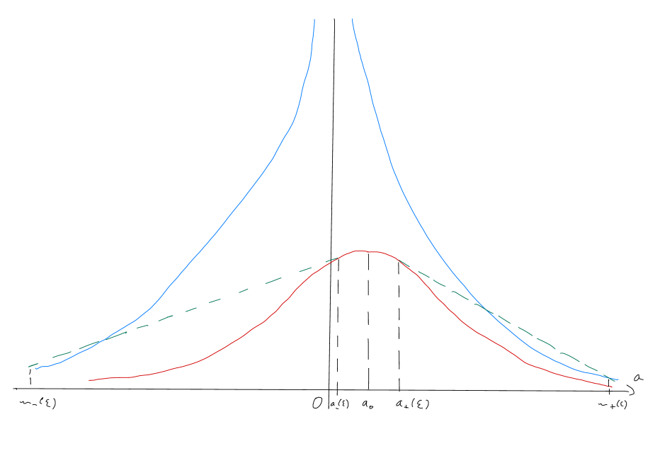
Figure 1: The mappings $\phi$ and $1/\beta$ are respectively in blue and red. The half-tangents with slope $-\varepsilon$ and $\varepsilon$ are in green.

The following observation will be important:

Lemma 20

We have

$$\lim_{\varepsilon\rightarrow 0_{+}}m_{+}(\varepsilon) = +\infty$$

$$\lim_{\varepsilon\rightarrow 0_{+}}m_{-}(\varepsilon) = -\infty$$

Proof

Fix any $M>2\beta(a_{0})$. Taking into account that

$$\lim_{\varepsilon\rightarrow 0_{+}}a_{+}(\varepsilon) = a_{0}$$

for $\varepsilon>0$ sufficiently small, we have

$$\frac{1}{\beta(a_{+}(\varepsilon))}-\varepsilon(M-a_{+}(\varepsilon)) > \frac{1}{2\beta(a_{0})}$$

$$> \phi(M)$$

It follows there exists $m\in(M,1/(a_{+}(\varepsilon)\varepsilon)+a_{+}(\varepsilon))$ such that

$$\frac{1}{\beta(a_{+}(\varepsilon))}-\varepsilon(m-a_{+}(\varepsilon)) = \phi(m)$$

and we deduce

$$\liminf_{\varepsilon\rightarrow 0_{+}}m_{+}(\varepsilon) \geq M$$

and finally the first desired divergence.

The second one is obtained in the same way.

$\blacksquare$

Consider the function $\theta$ defined on $\mathbb{R}$ by

$$\forall\ a\in\mathbb{R},\qquad\theta(a) \left\{\begin{array}[]{ll}\phi(a)&\hbox{, if $a<m_{-}(\varepsilon)$ or $a>m_{+}(\varepsilon)$}\\[5.69054pt] \displaystyle\frac{1}{\beta(a_{-}(\varepsilon))}+\varepsilon(a-a_{-}(\varepsilon))&\hbox{, if $a\in[m_{-}(\varepsilon),a_{-}(\varepsilon)]$}\\[11.38109pt] \displaystyle\frac{1}{\beta(a_{+}(\varepsilon))}-\varepsilon(a-a_{+}(\varepsilon))&\hbox{, if $a\in[a_{+}(\varepsilon),m_{+}(\varepsilon)]$}\\[11.38109pt] 1/\beta(a)&\hbox{, if $a\in[a_{-}(\varepsilon),a_{+}(\varepsilon)]$}\end{array}\right.$$

Lemma 21

We have

$$\forall\ a\in\mathbb{R}\setminus\{m_{-}(\varepsilon),m_{+}(\varepsilon)\},\qquad|\theta^{\prime}(a)| \leq \varepsilon$$

In particular, we get

$$\lim_{\varepsilon\rightarrow 0_{+}}\sup_{\mathbb{R}\setminus\{m_{-}(\varepsilon),m_{+}(\varepsilon)\}}|\theta^{\prime}| = 0$$

Proof

By construction, $\theta$ is differentiable on $\mathbb{R}$, except maybe at $m_{-}(\varepsilon)$ and $m_{+}(\varepsilon)$, where the left and right derivates may differ.

By definition of $a_{-}(\varepsilon)$ and $a_{+}(\varepsilon)$, we have

$$\forall\ a\in[a_{-}(\varepsilon),a_{+}(\varepsilon)],\qquad|\theta^{\prime}(a)|\ =\ |(1/\beta)^{\prime}(a)| \leq \varepsilon$$

Furthermore, note that

$$\forall\ a\in(m_{-}(\varepsilon),a_{-}(\varepsilon)]\sqcup[a_{+}(\varepsilon),m_{+}(\varepsilon)),\qquad|\theta^{\prime}(a)| = \varepsilon$$

Finally, we have

$$\forall\ a>m_{+}(\varepsilon),\qquad|\theta^{\prime}(a)| = |\phi^{\prime}(a)|$$

$$= \frac{1}{a^{2}}$$

so that

$$\forall\ a>m_{+}(\varepsilon),\qquad|\theta^{\prime}(a)| \leq \frac{1}{m_{+}^{2}(\varepsilon)}$$

and similarly

$$\forall\ a<m_{-}(\varepsilon),\qquad|\theta^{\prime}(a)| \leq \frac{1}{m_{-}^{2}(\varepsilon)}$$

We deduce $|\theta^{\prime}(a)|\leq\max(1/m^{2}_{-}(\varepsilon),1/m^{2}_{+}(\varepsilon),\varepsilon)$. To conclude to the desired bound, note that at $m_{+}(\varepsilon)$, we have

$$-\varepsilon \leq \phi^{\prime}(m_{+}(\varepsilon))\ \leq\ 0$$

since after $m_{+}(\varepsilon)$, $\phi$ is above the line of slope $-\varepsilon$ passing through $\phi(m_{+}(\varepsilon))$. Thus we get $1/m^{2}_{+}(\varepsilon)\leq\varepsilon$. Similarly we have $1/m^{2}_{-}(\varepsilon)\leq\varepsilon$ and the announced result follows.

$\blacksquare$

Let us check that for $\varepsilon>0$ small enough, $\theta$ remains above $1/\beta$.

Lemma 22

There exists $\varepsilon_{1}\in(0,\varepsilon_{0})$ such that for any $\varepsilon\in(0,\varepsilon_{1})$, we have $\theta\geq 1/\beta$.

Proof

To simplify the notation, let us write $q\df 1/\beta$ and let us work on $[a_{0},+\infty)$, similar arguments are valid on $(-\infty,a_{0}]$.

For $\varepsilon\in(0,\varepsilon_{0})$, define

$$c_{+}(\varepsilon) \min\left\{m>a_{+}(\varepsilon)\,:\,\frac{1}{\beta(a_{+}(\varepsilon))}-\varepsilon(m-a_{+}(\varepsilon))=\phi(m)\right\}$$

On $[a_{0},+\infty)$, it is clear from the definition of $\theta$ that $\theta\geq q$, except maybe on $[a_{+}(\varepsilon),c_{+}(\varepsilon)]$ (note that on $(c_{+}(\varepsilon),m_{+}(\varepsilon))$, $\theta\geq\phi\geq q$).

We have already seen that

$$\lim_{\varepsilon\rightarrow 0_{+}}a_{+}(\varepsilon) = a_{0}$$

and we have

$$\lim_{\varepsilon\rightarrow 0_{+}}c_{+}(\varepsilon) = c_{+}(0)$$ (30)

where $c_{+}(0)=1/q(a_{0})$ is the unique positive solution $a$ of $\phi(a)=q(a_{0})$.

We compute that

$$\forall\ a\in\mathbb{R},\qquad q^{\prime}(a) = \frac{1}{2}-(1+\frac{a^{2}}{2})q^{2}(a)$$ (31)

from which, we get

$$\forall\ a\in\mathbb{R},\qquad q^{\prime\prime}(a) = -aq^{2}(a)-2(1+\frac{a^{2}}{2})q(a)q^{\prime}(a)$$ (32)

Thus we can find $\varepsilon_{2}>0$ such that

$$\forall\ a\in[a_{0},a_{0}+\varepsilon_{2}],\qquad q^{\prime\prime}(a) \leq \frac{q^{\prime\prime}(a_{0})}{2}$$

$$= -a_{0}\frac{q^{2}(a_{0})}{2}\ <\ 0$$

Let $\varepsilon_{3}>0$ be such that for $\varepsilon\in(0,\varepsilon_{3})$, we have $a_{+}(\varepsilon)\in(a_{0},a_{0}+\varepsilon_{2}/2)$. By the strict concavity of $q$ on $[a_{0},a_{0}+\varepsilon_{2}]$, the affinity of $\theta$ on $[a+(\varepsilon),m_{+}(\varepsilon)]$ and the fact that $\theta^{\prime}(a_{+}(\varepsilon))=q^{\prime}(a_{+}(\varepsilon))$, we deduce that for $\varepsilon\in(0,\varepsilon_{3})$,

$$\forall\ a\in[a_{+}(\varepsilon),m_{+}(\varepsilon)\wedge(a_{0}+\varepsilon_{2})],\qquad\theta(a) \geq q(a)$$

Furthermore, up to reducing $\varepsilon_{3}>0$, we can assume that $m_{+}(\varepsilon)>a_{0}+\varepsilon_{2}$.

It remains to consider the situation on the segment $[a_{0}+\varepsilon_{2},c_{+}(\varepsilon)]$.

Taking into account (30) and the fact that the slope of $\theta$ tends to zero as $\varepsilon\rightarrow 0_{+}$, to show that $\theta\geq q$ on $[a_{0}+\varepsilon_{2},c_{+}(\varepsilon)]$ (for $\varepsilon\in(0,\varepsilon_{1})$ for some $\varepsilon_{1}\in(0,\varepsilon_{3})$), it is sufficient to show that $q^{\prime}<0$ on $(a_{0},+\infty)$.

By contradiction, assume there exists $a_{1}>a_{0}$ such that $q^{\prime}(a_{1})=0$. From (32), we deduce that

$$q^{\prime\prime}(a_{1}) = -a_{1}q^{2}(a_{1})\ <\ 0$$

From the fact that $q^{\prime}(a_{0})=0$ and $q^{\prime\prime}(a_{0})=-a_{0}q^{2}(a_{0})<0$, there must exist $a_{2}\in(a_{0},a_{1})$ with $q^{\prime}(a_{2})=0$ and $q^{\prime\prime}(a_{2})\geq 0$. This is in contradiction with the fact that $q^{\prime\prime}(a_{2})=-a_{2}q^{2}(a_{2})<0$.

$\blacksquare$

Fix $\varepsilon\in(0,\varepsilon_{1})$ and take $A>0$ large enough, so that $-A<m_{-}(\varepsilon)$ and $A>m_{+}(\varepsilon)$. For $n\geq A^{2}$, define the mapping $\xi_{n}$ on $[0,\pi]$ satisfying $\xi_{n}(0)=0$ and

$$\forall\ x\in(0,\pi),\qquad\xi_{n}^{\prime}(x) \left\{\begin{array}[]{ll}\frac{1}{\sqrt{n}}\theta\left(a\right)&\hbox{, if $a\in[-A,A]$}\\[5.69054pt] f_{n}(x)&\hbox{, otherwise}\end{array}\right.$$ (35)

(recall that $a=\sqrt{n}(x-\pi/2)$).

The function $\xi_{n}$ may not be strictly differentiable at $\pi/2-A/\sqrt{n}$ and $\pi/2+A/\sqrt{n}$ (the above formulas giving the right derivative at $-A$ and the left derivative at $A$), nor twice differentiable at $\pi/2-m_{-}(\varepsilon)/\sqrt{n}$ and $\pi/2+m_{+}(\varepsilon)/\sqrt{n}$. But outside these four points, $\xi_{n}$ is twice differentiable. Convoluting $\xi_{n}$ with an approximation of the Dirac mass at 0 and taking into account Lemma 21, we construct an increasing function $\psi_{n}$ twice differentiable on $(0,\pi)$ such that for $n$ large enough,

$$b_{n} \geq (1-\varepsilon)\frac{1}{\psi_{n}^{\prime}}$$ (36)

$$\sup_{(0,\pi)}|\psi_{n}^{\prime\prime}| \leq \varepsilon(1+\varepsilon)$$ (37)

Furthermore, the computations of Lemma 11 show that for large $n$,

$$\xi_{n}(\pi) \sim \frac{\ln(n)}{n}$$

thus for $n$ large enough,

$$\psi_{n}(\pi)-\psi_{n}(0) \leq (1+\varepsilon)\frac{\ln(n)}{n}$$ (38)

Taking into account that for $\varepsilon>0$ small enough, we have for $n$ large enough, $\psi_{n,+}\df\psi_{n}/(1-\epsilon)\in\Psi_{+}(\varphi_{n})$, we deduce from (23)

$$\limsup_{n\rightarrow\infty}\frac{n}{\ln(n)}\mathbb{E}[\tau_{n}] \leq \frac{1+\varepsilon}{1-\varepsilon-\varepsilon(1+\varepsilon)}$$

(where $\tau_{n}$ is the strong stationary time defined in (1)) and letting $\varepsilon$ go to zero, we conclude to the bound

$$\limsup_{n\rightarrow\infty}\frac{n}{\ln(n)}\mathbb{E}[\tau_{n}] \leq 1$$ (39)

To get a reverse bound, it is sufficient to apply (24) with appropriate avatars $\psi_{n,-}\in\Psi_{-}(\varphi_{n})$. Inspired by the computations of Section 2.2, we first take $A>0$ sufficiently large and consider the quantity $\epsilon(A)>0$ defined there. Up to choosing $A$ even larger, the above arguments are still valid, except that (36) and (38) can respectively be replaced by

$$b_{n} \leq (1+\varepsilon)\frac{1+\epsilon(A)}{\psi_{n}^{\prime}}$$

$$\psi_{n}(\pi)-\psi_{n}(0) \geq (1-\varepsilon)\frac{\ln(n)}{n}$$ (40)

It follows in particular that for $n$ large enough, $\psi_{n,-}\df\psi_{n}/[(1+\epsilon(A))(1+\varepsilon)]\in\Psi_{-}(\varphi_{n})$ and we deduce from (24),

$$\liminf_{n\rightarrow\infty}\frac{n}{\ln(n)}\mathbb{E}[\tau_{n}] \geq \frac{1-\varepsilon}{(1+\varepsilon)(1+\epsilon(A))-\varepsilon(1+\varepsilon)}$$

Letting $\varepsilon$ go to zero and $A$ to to $+\infty$, we deduce

$$\liminf_{n\rightarrow\infty}\frac{n}{\ln(n)}\mathbb{E}[\tau_{n}] \geq 1$$

In conjunction with (39), this ends the proof of Theorem 2.

To end this section, let us show Theorem 3.

We begin by its first convergence, where $r>0$ is fixed from now on.

For $\varepsilon>0$ sufficiently small, consider again the mapping $\psi_{n,+}\in\Psi_{+}(\varphi_{n})$ defined above. According to (25), we have for any $r>0$,

$$\mathbb{P}\left[\tau_{n}>\frac{\psi_{n,+}(\pi)-\psi_{n,+}(0)}{1+\min_{[0,\pi]}\psi_{n,+}^{\prime\prime}}(1+r/2)\right] \leq \frac{4}{r^{2}(\psi_{n,+}(\pi)-\psi_{n,+}(0))^{2}(1+3\min_{[0,\pi]}\psi_{n,+}^{\prime\prime})}\int_{0}^{\pi}(\psi_{n,+}^{\prime}(u))^{3}\,du$$

Up to choosing $\varepsilon>0$ even smaller, (37) and (38) insure that for all $n$ sufficiently large, we have

$$\frac{\psi_{n,+}(\pi)-\psi_{n,+}(0)}{1+\min_{[0,\pi]}\psi_{n,+}^{\prime\prime}}(1+r/2) < (1+r)\frac{\ln(n)}{n}$$

implying

$$\mathbb{P}\left[\tau_{n}>(1+r)\frac{\ln(n)}{n}\right] \leq \frac{4}{r^{2}(\psi_{n,+}(\pi)-\psi_{n,+}(0))^{2}(1+3\min_{[0,\pi]}\psi_{n,+}^{\prime\prime})}\int_{0}^{\pi}(\psi_{n,+}^{\prime}(u))^{3}\,du$$

Thus the first convergence of Theorem 3 is a consequence of (4) and

Lemma 23

We have

$$\lim_{n\rightarrow\infty}\frac{n^{2}}{\ln^{2}(n)}\int_{0}^{\pi}(\psi_{n,+}^{\prime}(u))^{3}\,du = 0$$

Proof

The above convergence is equivalent to

$$\lim_{n\rightarrow\infty}\frac{n^{2}}{\ln^{2}(n)}\int_{0}^{\pi}(\psi_{n}^{\prime}(u))^{3}\,du = 0$$ (41)

Since differentiation and convolution commute and convolution is a contraction in $\mathbb{L}^{p}$, for $p\geq 1$ (recall that $\psi_{n}^{\prime}>0$), (41) is itself implied by

$$\lim_{n\rightarrow\infty}\frac{n^{2}}{\ln^{2}(n)}\int_{0}^{\pi}(\xi_{n}^{\prime}(u))^{3}\,du = 0$$ (42)

Coming back to Definition (35), we write

$$\int_{0}^{\pi}(\xi_{n}^{\prime}(u))^{3}\,du = \int_{(0,\pi)\setminus[\pi/2-A/\sqrt{n},\pi/2+A/\sqrt{n}]}(\xi_{n}^{\prime}(u))^{3}\,du+\int_{[\pi/2-A/\sqrt{n},\pi/2+A/\sqrt{n}]}(\xi_{n}^{\prime}(u))^{3}\,du$$

$$= \frac{1}{n^{3}}\int_{(0,\pi)\setminus[\pi/2-A/\sqrt{n},\pi/2+A/\sqrt{n}]}|\tan(u)|^{3}\,du+\frac{1}{n^{2}}\int_{-A}^{A}\theta^{3}(a)\,da$$

Note that the first term of the r.h.s. si equal to

$$\frac{2}{n^{3}}\int_{0}^{\pi/2-A/\sqrt{n}}\tan^{3}(u)\,du = \frac{2}{n^{3}}\int_{A/\sqrt{n}}^{\pi/2}\cot^{3}(u)\,du$$

$$\leq \frac{2}{n^{3}}\int_{A/\sqrt{n}}^{\pi/2}\frac{1}{u^{3}}\,du$$

$$= \frac{1}{n^{3}}\left[-\frac{1}{u^{2}}\right]_{A/\sqrt{n}}^{\pi/2}$$

$$\leq \frac{1}{n^{3}}\frac{n}{A^{2}}\ =\ \frac{1}{(An)^{2}}$$

and thus

$$\frac{n^{2}}{\ln^{2}(n)}\frac{1}{n^{3}}\int_{(0,\pi)\setminus[\pi/2-A/\sqrt{n},\pi/2+A/\sqrt{n}]}|\tan(u)|^{3}\,du \leq \frac{1}{(A\ln(n))^{2}}$$

converging toward 0 for large $n$.

Similarly we have

$$\frac{n^{2}}{\ln^{2}(n)}\frac{1}{n^{2}}\int_{-A}^{A}\theta^{3}(a)\,da = \frac{1}{\ln^{2}(n)}\int_{-A}^{A}\theta^{3}(a)\,da$$

converging toward 0 for large $n$ and ending the proof of (42).

$\blacksquare$

The proof of the second convergence of Theorem 3 follows a similar pattern, via (26) applied to $\psi_{n,-}\in\Psi_{-}(\varphi_{n})$.

Indeed, $r\in(0,1)$ being fixed, we first find $A>0$ sufficiently large and $\varepsilon>0$ sufficiently small so that for all large enough $n$,

$$\frac{\psi_{n,-}(\pi)-\psi_{n,-}(0)}{1+\min_{[0,\pi]}\psi_{n,-}^{\prime\prime}}(1-r/2) > (1-r)\frac{\ln(n)}{n}$$

and we get

$$\mathbb{P}\left[\tau_{n}<(1-r)\frac{\ln(n)}{n}\right] \leq \frac{4}{r^{2}(\psi_{n,-}(\pi)-\psi_{n,-}(0))^{2}(1+3\min_{[0,\pi]}\psi_{n,-}^{\prime\prime})}\int_{0}^{\pi}(\psi_{n,-}^{\prime}(u))^{3}\,du$$

This bound implies the second convergence of Theorem 3 via the analogue of Lemma 23, where $\psi_{n,+}$ is replaced by $\psi_{n,-}$, and which is proven in exactly the same way.

We also deduce the following consequences from the proof of Lemma 23:

Corollary 24

For any $x\in\SS^{n+1}$, let $X^{x}\df(X_{t}^{x})_{t\geq 0}$ be the Brownian motion on the sphere $\SS^{n+1}$ (time-accelerated by a factor $2$), starting with $X^{x}_{0}=x$. There exist $C>0$ and $n_{0}\in\mathbb{N}$ such that for all $r>0$ and for all $n\geq n_{0}$,

$$\left\|\mathcal{L}\left(X^{x}_{(1+r)\frac{\ln(n)}{n}}\right)-\mu_{\SS^{n+1}}\right\|_{\mathrm{tv}} \leq \frac{C}{r^{2}\ln^{2}(n)}$$

$$\forall\ y\in\SS^{n+1},\qquad P^{(n+1)}_{(1+r)\frac{\ln(n)}{n}}(x,y) \geq \left(1-\frac{C}{r^{2}\ln^{2}(n)}\right)\frac{1}{\mathrm{vol}(\SS^{n+1})}$$

where $\|\cdot\|_{\mathrm{tv}}$ stands for the total variation norm, $\mathcal{L}(X^{x}_{t})$ is the law of $X^{x}_{t}$, $\mu_{\SS^{n+1}}$ is the uniform measure in $\SS^{n+1}$, and $P^{(n+1)}_{t}(\cdot,\cdot)$ is the heat kernel density at time $t>0$ associated to the Laplacian on $\SS^{n+1}$.

Proof

From the computations in the proof of Lemma 23, there exist a constant $C$ depending on the quantity $\max\{\int_{-A}^{A}\theta^{3}(a)\,da,\frac{1}{A^{2}}\}$, and $n_{0}\in\mathbb{N}$ such that for all $n\geq n_{0}$,

$$\mathbb{P}\left[\tau_{n}>(1+r)\frac{\ln(n)}{n}\right] \leq \frac{C}{r^{2}\ln^{2}(n)}$$

The first conclusion follows, since

$$\left\|\mathcal{L}\left(X^{x}_{(1+r)\frac{\ln(n)}{n}}\right)-\mu_{\SS^{n+1}}\right\|_{\mathrm{tv}} \leq \mathfrak{s}\left(\mathcal{L}\left(X^{x}_{(1+r)\frac{\ln(n)}{n}}\right),\mu_{\SS^{n+1}}\right)\ \leq\ \mathbb{P}\left[\tau_{n}>(1+r)\frac{\ln(n)}{n}\right]$$

The second conclusion follows by definition of the separation discrepancy, since for all $y\in\SS^{n+1}$ and $t>0$,

$$1-P^{(n+1)}_{t}(x,y)\mathrm{vol}(\SS^{n+1}) \leq \mathfrak{s}(\mathcal{L}(X^{x}_{t}),\mu_{\SS^{n+1}})$$

$\blacksquare$

5 On the necessity of avatars

Our goal here is to see the bound given in (23) can be strictly better than Lemma 15.

Indeed, it will a consequence of the following result.

For any $n\in\mathbb{N}$, consider the function $\varphi_{n}$ defined on $[0,\pi]$ satisfying $\varphi_{n}(0)=0$ and

$$\forall\ x\in(0,\pi),\qquad\varphi^{\prime}_{n}(x) \frac{1}{b_{n}(x)}$$

$$= \frac{\sin(x)I_{n}(x)}{2\sin^{n+1}(x)-n\cos(x)I_{n}(x)}$$

From the computations of Section 2, we have for large $n$,

$$\varphi_{n}(\pi) \sim \frac{\ln(n)}{n}$$

But we have:

Proposition 25

The limit $\lim_{n\rightarrow\infty}\min_{[0,\pi]}\varphi_{n}^{\prime\prime}$ exists and its value belongs to $[-5/11,-1/7]$.

Thus Lemma 15 alone would not have permitted us to prove Theorem 2.

On the two following subsections, we respectively investigate $\varphi_{n}^{\prime\prime}$ on $[0,\pi/2]$ and $[\pi/2,\pi]$.

5.1 On $[0,\pi/2]$

Before investigating the minimum of $\varphi_{n}^{\prime\prime}$ on $[0,\pi/2]$, we start with some considerations valid on $[0,\pi]$. For any $x\in[0,\pi]$, we have

$$\cos(x)I_{n}(x) \leq \int_{0}^{x}\cos(u)\sin^{n}(u)\,du$$ (43)

$$= \left[\frac{\sin^{n+1}(u)}{n+1}\right]_{0}^{x}$$

$$= \frac{\sin^{n+1}(x)}{n+1}$$

We deduce that the denominator of $\varphi_{n}^{\prime}(x)$ satisfies

$$2\sin^{n+1}(x)-n\cos(x)I_{n}(x) \geq 2\sin^{n+1}(x)-n\frac{\sin^{n+1}(x)}{n+1}$$

$$= \frac{n+2}{n+1}\sin^{n+1}(x)$$

which stays positive on $(0,\pi)$.

Furthermore, as $x$ tends to $0_{+}$, we have

$$2\sin^{n+1}(x)-n\cos(x)I_{n}(x) \sim \frac{n+2}{n+1}\sin^{n+1}(x)$$ (44)

so that

$$\varphi_{n}^{\prime}(x) \sim \frac{x}{n+2}$$

$$\rightarrow 0$$

At the other boundary $\pi$, we get

$$\varphi_{n}^{\prime}(x) \sim -\frac{I_{n}(\pi)\sin(x)}{nI_{n}(\pi)}$$

$$\rightarrow 0$$

We compute for any $x\in(0,\pi)$,

$$\varphi_{n}^{\prime\prime}(x) = \frac{\sin^{n+1}(x)+\cos(x)I_{n}(x)}{2\sin^{n+1}(x)-n\cos(x)I_{n}(x)}$$

$$-\frac{\sin(x)I_{n}(x)[2(n+1)\cos(x)\sin^{n}(x)+n\sin(x)I_{n}(x)-n\cos(x)\sin^{n}(x)]}{(2\sin^{n+1}(x)-n\cos(x)I_{n}(x))^{2}}$$

$$= \frac{2\sin^{2(n+1)}(x)-2n\cos(x)\sin^{n+1}(x)I_{n}(x)-nI_{n}^{2}(x)}{(2\sin^{n+1}(x)-n\cos(x)I_{n}(x))^{2}}$$

Let us rewrite $\varphi_{n}^{\prime\prime}(x)=N(x)/D^{2}(x)$ with

$$N(x) 2-2n\cos(x)J_{n}(x)-nJ_{n}^{2}(x)$$

$$D(x) 2-n\cos(x)J_{n}(x)$$

with

$$J_{n}(x) \frac{I_{n}(x)}{\sin^{n+1}(x)}$$

Here are some observations on this function

Lemma 26

We have

$$J_{n}^{\prime}(x) = \frac{1}{\sin(x)}(1-(n+1)\cos(x)J_{n}(x))$$

and in particular $J_{n}$ is increasing on $(0,\pi)$.

Proof

Indeed, we compute

$$J_{n}^{\prime}(x) = \frac{\sin^{n}(x)\sin^{n+1}(x)-(n+1)\cos(x)\sin^{n}(x)I_{n}(x)}{\sin^{2(n+1)}(x)}$$

$$= \frac{1}{\sin(x)}(1-(n+1)\cos(x)J_{n}(x))$$

From inequality (43), we get that for any $x\in(0,\pi)$, $J_{n}^{\prime}(x)\geq 0$ on $(0,\pi)$.

$\blacksquare$

Since the first bound in (43) is an equivalent for small $x$, we also get

$$\lim_{x\rightarrow 0_{+}}J_{n}(x) = \frac{1}{n+1}$$

and thus

$$\lim_{x\rightarrow 0_{+}}N(x) = 2-\frac{2n}{n+1}-n\frac{1}{(n+1)^{2}}$$

$$= \frac{2(n+1)^{2}-2n(n+1)-n}{(n+1)^{2}}$$

$$= \frac{n+2}{(n+1)^{2}}$$

We now restrict our attention to the case where $x\in(0,\pi/2)$.

Lemma 27

We have

$$\forall\ x\in(0,\pi/2),\qquad N(x) \geq 0$$

Proof

We compute that for any $x\in(0,\pi)$,

$$N^{\prime}(x) = 2n\sin(x)J_{n}(x)-2n\cos(x)J_{n}^{\prime}(x)-2nJ_{n}(x)J_{n}^{\prime}(x)$$

$$= 2n\sin(x)J_{n}(x)-2n(\cos(x)+J_{n}(x))\frac{1}{\sin(x)}(1-(n+1)\cos(x)J_{n}(x))$$

$$= \frac{2n}{\sin(x)}\left(\sin^{2}(x)J_{n}(x)-(\cos(x)+J_{n}(x))(1-(n+1)\cos(x)J_{n}(x))\right)$$

$$= \frac{2n\cos(x)}{\sin(x)}\left(-1+n\cos(x)J_{n}(x)+(n+1)J_{n}^{2}(x)\right)$$

Assume there exists some $x_{0}\in(0,\pi/2)$ such that $N(x_{0})=0$, namely

$$2-2n\cos(x_{0})J_{n}(x_{0})-nJ_{n}^{2}(x_{0}) = 0$$

then we get

$$-1+n\cos(x_{0})J_{n}(x_{0})+(n+1)J_{n}^{2}(x_{0}) = -1+n\cos(x_{0})J_{n}(x_{0})+\frac{n+1}{n}(2-2n\cos(x_{0})J_{n}(x_{0}))$$

$$= \frac{n+2}{n}-(n+2)\cos(x_{0})J_{n}(x_{0})$$

$$\geq \frac{n+2}{n}-\frac{n+2}{n+1}$$

$$> 0$$

From this observation we get $N^{\prime}(x_{0})>0$ and in conjunction with the fact that

$$N(0) = \frac{n+2}{(n+1)^{2}}\ >\ 0$$

we deduce that $N$ remains non-negative on $(0,\pi/2)$.

$\blacksquare$

It follows that

$$\min_{[0,\pi/2]}\varphi_{n}^{\prime\prime} \geq 0$$ (45)

5.2 On $[\pi/2,\pi]$

We study here the minimum of $\varphi_{n}^{\prime\prime}$ on $[\pi/2,\pi]$.

Let us change the notations of the previous section and rather write for $x\in(0,\pi)$,

$$\varphi_{n}^{\prime\prime}(x) = \frac{N(x)}{D^{2}(x)}$$

where

$$N(x) 2\sin^{2(n+1)}(x)-2n\cos(x)\sin^{n+1}(x)I_{n}(x)-nI_{n}^{2}(x)$$

$$D(x) 2\sin^{n+1}(x)-n\cos(x)I_{n}(x)$$

As in Section 2, fix some $A>0$, and for $n>A^{2}$, we consider the parametrization $x=\pi/2+a/\sqrt{n}$ with $a\in[0,A]$. Taking into account Lemma 10, introduce the functions $\nu$ and $\delta$ defined on $\mathbb{R}_{+}$ via

$$\forall\ a\geq 0,\qquad\left\{\begin{array}[]{rcl}\nu(a)&\df\hfil&2e^{-a^{2}}+2ae^{-a^{2}/2}h(a)-h^{2}(a)\\[5.69054pt] \delta(a)&\df\hfil&2e^{-a^{2}/2}+ah(a)\end{array}\right.$$

We get for large $n$, uniformly over $a\in[0,A]$,

$$N(x) \sim \nu(a)$$

$$D(x) \sim \delta(a)$$

(except that if $\nu(a)=0$ the first equivalence must be replaced by $\lim_{n\rightarrow\infty}N(x)=0$).

Taking into account that our equivalences are up to a factor of the form $1+\mathcal{O}_{a}(1/\sqrt{n})$ where the bounding factor in the Landau notation $\mathcal{O}_{a}$ is uniform over $a\in[0,A]$, we deduce that uniformly over $a\in[0,A]$,

$$\lim_{n\rightarrow\infty}\varphi_{n}^{\prime\prime}(x) = \chi(a)\ \df\ \frac{\nu(a)}{\delta^{2}(a)}$$

Here are the variation of the function $\chi$:

Lemma 28

There exists $a_{0}>0$ such that $\chi$ is decreasing on $[0,a_{0}]$ and increasing on $[a_{0},+\infty)$. This $a_{0}$ is the unique solution of

$$(2+a_{0}^{2})e^{-a_{0}^{2}}+a_{0}(3+a_{0}^{2})e^{-a_{0}^{2}/2}h(a_{0})-h^{2}(a_{0}) = 0$$ (47)

Proof

We have that for any $a>0$,

$$\chi^{\prime}(a) = \frac{\nu^{\prime}(a)\delta(a)-2\nu(a)\delta^{\prime}(a)}{\delta^{3}(a)}$$

and we want to show that there exists a unique $a_{0}>0$ such that $\chi^{\prime}(a_{0})=0$ and that furthermore $\chi^{\prime}$ is negative on $(0,a_{0})$ and positive on $(a_{0},+\infty)$.

We compute

$$\nu^{\prime}(a) = -4ae^{-a^{2}}+2e^{-a^{2}/2}h(a)-2a^{2}e^{-a^{2}/2}h(a)+2ae^{-a^{2}}-2e^{-a^{2}/2}h(a)$$

$$= -2ae^{-a^{2}}-2a^{2}e^{-a^{2}/2}h(a)$$

$$\delta^{\prime}(a) = -2ae^{-a^{2}/2}+h(a)+ae^{-a^{2}/2}$$

$$= -ae^{-a^{2}/2}+h(a)$$

and thus

$$(\nu^{\prime}\delta-2\nu\delta^{\prime})(a) = (-2ae^{-a^{2}}-2a^{2}e^{-a^{2}/2}h(a))(2e^{-a^{2}/2}+ah(a))$$

$$-2(2e^{-a^{2}}+2ae^{-a^{2}/2}h(a)-h^{2}(a))(-ae^{-a^{2}/2}+h(a))$$

$$= -2h(a)\xi(a)$$

with

$$\forall\ a\geq 0,\qquad\xi(a) (2+a^{2})e^{-a^{2}}+a(3+a^{2})e^{-a^{2}/2}h(a)-h^{2}(a)$$ (48)

Our goal amounts to find a unique $a_{0}>0$ such that $\xi(a_{0})=0$ and that furthermore $\xi$ is positive on $(0,a_{0})$ and negative on $(a_{0},+\infty)$. Let us differentiate: for any $a>0$,

$$\xi^{\prime}(a) = a(1-a^{2})e^{-a^{2}}+(1-a^{4})e^{-a^{2}/2}h(a)$$

It appears that $\xi$ is increasing on $(0,1)$ and decreasing on $(1,+\infty)$. Since

$$\xi(0) = 2-\sqrt{\frac{\pi}{2}}\ >\ 0$$

$$\lim_{a\rightarrow+\infty}\xi(a) = -2\pi\ <\ 0$$

we deduce the desired result on $\xi$.

$\blacksquare$

Note that

$$\lim_{a\rightarrow+\infty}\chi(a) = 0$$

so that $\chi(a_{0})<0$. As a consequence we get

Proposition 29

We have

$$\lim_{n\rightarrow\infty}\inf_{x\in[\pi/2,\pi]}\varphi_{n}^{\prime\prime}(x) = \chi(a_{0})$$

Proof

Fix $A>a_{0}$ and for $n>A^{2}$, consider $x_{n}$ such that $\cos(x_{n})=-A/\sqrt{n}$. For any $x\in[x_{n},\pi]$, we have

$$\varphi_{n}^{\prime\prime}(x) \geq \frac{-nI^{2}_{n}(x)}{(n\cos(x)I_{n}(x))^{2}}$$

$$= -\frac{1}{n\cos^{2}(x)}$$

$$\geq -\frac{1}{n\cos^{2}(x_{n})}$$

$$= -\frac{1}{A^{2}}$$

We get

$$\inf_{x\in[x_{n},\pi]}\varphi_{n}^{\prime\prime}(x) \geq -\frac{1}{A^{2}}$$

From Lemma 28 and since $A>a_{0}$, we have

$$\lim_{n\rightarrow\infty}\inf_{x\in[\pi/2,x_{n}]}\varphi_{n}^{\prime\prime}(x) = \chi(a_{0})$$ (49)

By choosing furthermore $A>a_{0}$ such that $1/A^{2}<|\chi(a_{0})|$, we deduce

$$\inf_{x\in[\pi/2,\pi]}\varphi_{n}^{\prime\prime}(x) = \inf_{x\in[\pi/2,x_{n}]}\varphi_{n}^{\prime\prime}(x)\wedge\inf_{x\in[x_{n},\pi]}\varphi_{n}^{\prime\prime}(x)$$

$$= \inf_{x\in[\pi/2,x_{n}]}\varphi_{n}^{\prime\prime}(x)$$

for $n$ large enough. The announced result now follows from (49).

$\blacksquare$

Taking into account (45), we get

$$\lim_{n\rightarrow\infty}\inf_{x\in[0,\pi]}\varphi_{n}^{\prime\prime}(x) = \chi(a_{0})$$

implying in particular the first statement of Proposition 25.

Let us show its last statement.

Extracting $h^{2}(a_{0})$ from (47):

$$h^{2}(a_{0}) = (2+a_{0}^{2})e^{-a_{0}^{2}}+a_{0}(3+a_{0}^{2})e^{-a_{0}^{2}/2}h(a_{0})$$

and replacing first in $\nu(a_{0})$:

$$\nu(a_{0}) = 2e^{-a_{0}^{2}}+2a_{0}e^{-a_{0}^{2}/2}h(a_{0})-h^{2}(a_{0})$$

$$= 2e^{-a_{0}^{2}}+2a_{0}e^{-a_{0}^{2}/2}h(a_{0})-[(2+a_{0}^{2})e^{-a_{0}^{2}}+a_{0}(3+a_{0}^{2})e^{-a_{0}^{2}/2}h(a_{0})]$$

$$= -a_{0}^{2}e^{-a_{0}^{2}}-a_{0}(1+a_{0}^{2})e^{-a_{0}^{2}/2}h(a_{0})$$

and next in $\delta^{2}(a_{0})$:

$$\delta^{2}(a_{0}) = 4e^{-a_{0}^{2}}+4a_{0}e^{-a^{2}_{0}/2}h(a_{0})+a_{0}^{2}h^{2}(a_{0})$$

$$= 4e^{-a_{0}^{2}}+4a_{0}e^{-a^{2}_{0}/2}h(a_{0})+a_{0}^{2}[(2+a_{0}^{2})e^{-a_{0}^{2}}+a_{0}(3+a_{0}^{2})e^{-a_{0}^{2}/2}h(a_{0})]$$

$$= (4+2a_{0}^{2}+a_{0}^{4})e^{-a_{0}^{2}}+(7a_{0}+a_{0}^{3})e^{-a_{0}^{2}/2}h(a_{0})$$

we deduce

$$-\chi(a_{0}) = \frac{a_{0}^{2}e^{-a_{0}^{2}}+a_{0}(1+a_{0}^{2})e^{-a_{0}^{2}/2}h(a_{0})}{(4+2a_{0}^{2}+a_{0}^{4})e^{-a_{0}^{2}}+(7a_{0}+a_{0}^{3})e^{-a_{0}^{2}/2}h(a_{0})}$$

$$\in \left[\frac{a_{0}^{2}}{4+2a_{0}^{2}+a_{0}^{4}}\wedge\frac{1+a_{0}^{2}}{7+a_{0}^{2}},\frac{a_{0}^{2}}{4+2a_{0}^{2}+a_{0}^{4}}\vee\frac{1+a_{0}^{2}}{7+a_{0}^{2}}\right]$$

Recalling (48), it is immediate to compute that $\xi(1)>0$ while $\xi(2)<0$, implying that $a_{0}\in(1,2)$. It follows that

$$\frac{1+a_{0}^{2}}{7+a_{0}^{2}} = 1-\frac{6}{7+a_{0}^{2}}$$

$$\in \left[1-\frac{6}{7+1^{2}},1-\frac{6}{7+2^{2}}\right]$$

$$= \left[\frac{1}{4},\frac{5}{11}\right]$$

Remarking that the mapping $a\mapsto a^{2}/(4+2a^{2}+a^{4})$ is increasing on $[1,\sqrt{2}]$ and decreasing on $[\sqrt{2},2]$, we furthermore get

$$\frac{a_{0}^{2}}{4+2a_{0}^{2}+a_{0}^{4}} \in \left[\frac{1^{2}}{4+2\times 1^{2}+1^{4}}\wedge\frac{2^{2}}{4+2\times 2^{2}+2^{4}},\frac{2}{4+2\times 2+2^{2}}\right]$$

$$= \left[\frac{1}{7},\frac{1}{6}\right]$$

The wanted bounds follow:

$$-\chi(a_{0}) \in \left[\frac{1}{7},\frac{5}{11}\right]$$

marc.arnaudon@math.u-bordeaux.fr

Institut de Mathématiques de Bordeaux

F. 33405, Talence, France

kolehe.coulibaly@univ-lorraine.fr

Institut Élie Cartan de Lorraine

Université de Lorraine

miclo@math.cnrs.fr

Toulouse School of Economics

1, Esplanade de l’université

31080 Toulouse cedex 06, France

References

[1]
Marc Arnaudon, Koléhè Coulibaly-Pasquier, and Laurent Miclo.
Construction of set-valued dual processes on manifolds.
preprint, December 2020.
[2]
Koléhè Coulibaly-Pasquier and Laurent Miclo.
On the evolution by duality of domains on manifolds.
Mém. Soc. Math. Fr., Nouv. Sér., 171:1–110, 2021.
[3]
Persi Diaconis.
The cutoff phenomenon in finite Markov chains.
Proc. Nat. Acad. Sci. U.S.A., 93(4):1659–1664, 1996.
[4]
Persi Diaconis and James Allen Fill.
Strong stationary times via a new form of duality.
Ann. Probab., 18(4):1483–1522, 1990.
[5]
Persi Diaconis and Laurent Saloff-Coste.
Separation cut-offs for birth and death chains.
Ann. Appl. Probab., 16(4):2098–2122, 2006.
[6]
Jian Ding, Eyal Lubetzky, and Yuval Peres.
Total variation cutoff in birth-and-death chains.
Probab. Theory Relat. Fields, 146(1-2):61–85, 2010.
[7]
Jonathan Hermon, Hubert Lacoin, and Yuval Peres.
Total variation and separation cutoffs are not equivalent and neither
one implies the other.
Electron. J. Probab., 21:36, 2016.
Id/No 44.
[8]
David A. Levin, Yuval Peres, and Elizabeth L. Wilmer.
Markov chains and mixing times.
American Mathematical Society, Providence, RI, 2009.
With a chapter by James G. Propp and David B. Wilson.
[9]
Pierre-Loïc Méliot.
The cut-off phenomenon for Brownian motions on compact symmetric
spaces.
Potential Anal., 40(4):427–509, 2014.
[10]
L. Saloff-Coste.
Precise estimates on the rate at which certain diffusions tend to
equilibrium.
Math. Z., 217(4):641–677, 1994.