Standard symmetrized variance with applications to coherence, uncertainty and entanglement

Abstract

Variance is a ubiquitous quantity in quantum information theory. Given a basis, we consider the averaged variances of a fixed diagonal observable in a pure state under all possible permutations on the components of the pure state and call it the symmetrized variance. Moreover we work out the analytical expression of the symmetrized variance and find that such expression is in the factorized form where two factors separately depends on the diagonal observable and quantum state. By shifting the factor corresponding to the diagonal observable, we introduce the notion named the standard symmetrized variance for the pure state which is independent of the diagonal observable. We then extend the standard symmetrized variance to mixed states in three different ways, which characterize the uncertainty, the coherence and the coherence of assistance, respectively. These quantities are evaluated analytically and the relations among them are established. In addition, we show that the standard symmetrized variance is also an entanglement measure for bipartite systems. In this way, these different quantumness of quantum states are unified by the variance.

I Introduction

Measuring statistically the deviation of measurement outcomes from the ideal value of quantum measurements on given quantum states, the variance plays an important role in quantum physics and quantum information theory. The first uncertainty relation known as the Heisenberg’s uncertainty relation was given in terms of the variance W. Heisenberg ; H. P. Robertson , which describes the restrictions on the accuracy of measurement results of two or more noncommutative observables. Since then, many efforts are made to find tighter and state-independent lower bounds on such kind of uncertainty relations Pati2014 ; S. Friedland ; Schwonnek2017 . In order to study the restriction between the uncertainties for two or more observables, the notion of the uncertainty region is also put forward and characterized Werner2015 ; Zhang2021 .

For any given mixed state and observable, it has been shown that the minimal averaged variance among all possible pure-state decompositions is exactly the quantum Fisher information and the maximal averaged variance is the variance itself Yu2013 ; Toth2013 ; S. Braunstein ; G. Toth2017 . Concerning the relation between the variance and quantum Fisher information, the improved uncertainty relations have been derived in terms of quantum Fisher information and variance S. Luo2005pra ; Toth2021 ; Gessner2021 . Moreover, the variance-based uncertainty relation has been incorporated into quantum multiparameter estimation by investigating the quantum Fisher information matrix and the classical Fisher information matrix from measurements Lu2021 . It is well known that the quantum Fisher information places the fundamental limit to the accuracy for estimating an unknown parameter and plays an important role in quantum metrology. The uncertainty relation and quantum metrology are then closely connected by the variance and quantum Fisher information.

More than that, the variance can also be used to detect quantum entanglement Schwonnek2017 ; H. F. Hofmann ; O. Guhne ; N. Li2013 ; Y. Hong and quantify quantum coherence Y. Zhang2020 ; Li2021 ; Xu2021 . In view of the importance of the variance in quantum information theory, we aim to explore the role played by the variance, as a unifying tool, in characterizing the quantumness. In a $d$-dimensional system with fixed basis $\{|i\rangle:i=0,1,\ldots,d-1\}$, any pure state can be expressed as $|\psi\rangle=\sum_{i=0}^{d-1}\psi_{i}|i\rangle$. Since the quantumness of the pure state is invariant under relabeling the coefficients $\{\psi_{i}\}$, in order to study the quantumness of the pure state $|\psi\rangle$, one may consider the averaged quantumness in the set of pure states $\{\bm{P}_{\pi}|\psi\rangle\}$, where $\bm{P}_{\pi}$ are all possible permutation matrices corresponding to the permutations $\pi$ of the permutation group $S_{d}$. In this context, we propose the averaged variances of any diagonal observable over the set of $\{\bm{P}_{\pi}|\psi\rangle\}$ and named as symmetrized variance $\widehat{\operatorname{Var}}(|\psi\rangle,\bm{A})$. By analysis and calculation, we obtain the analytical expression of the symmetrized variance and find that the information of the pure state and the diagonal observable are factorized. By shifting the information of the diagonal observable, we introduce the core notion of this paper called the standard symmetrized variance $\widehat{V}(|\psi\rangle)$.

Although the standard symmetrized variance is in terms of variance, we find that it is independent of the diagonal observable and just depends on the pure state itself. Namely, the standard symmetrized variance describes the quantumness in the pure state. We generalize the standard symmetrized variance from the pure states to mixed states based on three different extensions. The first extension is the standard symmetrized variance $\widehat{V}(\rho)$ obtained by replacing the pure state with mixed ones directly. We get the analytical formula of $\widehat{V}(\rho)$ and show that it is a measure of uncertainty associated to the state $\rho$. The second extension is the convex roof extension $\widehat{V}_{c}(\rho)$. The lower bound of $\widehat{V}_{c}(\rho)$ is derived in terms of the eigenvalues and eigenvectors of the mixed state, which can be attained for qubit quantum states. The convex roof extension $\widehat{V}_{c}(\rho)$ is a coherence measure for $\rho$. The third extension is the concave bottom extension $\widehat{V}_{a}(\rho)$, which, dual to $\widehat{V}_{c}(\rho)$, is the coherence of assistance. These three extensions are depicted in Bloch ball for any qubit state. The standard symmetrized variance can also give rise to an entanglement measure in bipartite systems. The schematic on the relations among these quantities is given in Fig. 1.

Figure 1: The diagram of the standard symmetrized variances. $\operatorname{Var}(|\psi\rangle,\bm{A})$ is the variance of the diagonal observable $\bm{A}$ in the pure state $|\psi\rangle$ defined in Eq. (1). $\widehat{\operatorname{Var}}(|\psi\rangle,\bm{A})$ is the symmetrized variance of the diagonal observable $\bm{A}$ in the pure state $|\psi\rangle$ defined in Eq. (II.1). $\widehat{V}(|\psi\rangle)$ is the standard symmetrized variance of the pure state $|\psi\rangle$ defined in Eq. (4). $\widehat{V}(\rho)$ is the standard symmetrized variance of the mixed state $\rho$ defined in Eq. (6), which is an uncertainty measure. $\widehat{V}_{c}(\rho)$ is the convex roof extension of the standard symmetrized variance defined in Eq. (9), which is a coherence measure. $\widehat{V}_{a}(\rho)$ is the concave bottom extension of the standard symmetrized variance defined in Eq. (12), which is the coherence of assistance.

II The standard symmetrized variance

For any quantum state $\rho$ and an observable $\bm{A}$ in a $d$-dimensional system, the variance

$$\operatorname{Var}(\rho,\bm{A})=\operatorname{Tr}\left(\bm{A}^{2}\rho\right)-[\operatorname{Tr}\left(\bm{A}\rho\right)]^{2}$$

is a measure of uncertainty of the observable $\bm{A}$ in the state $\rho$. In this paper, we fix the reference basis as $\{|i\rangle:i=0,1,\ldots,d-1\}$ and just consider the variance of diagonal observables $\bm{A}$ in quantum state $\rho$ throughout this paper.

II.1 Standard symmetrized variance for pure states

For any pure state $|\psi\rangle=\sum_{i=0}^{d-1}\psi_{i}|i\rangle$, the vector $\left(r_{0},r_{1},\ldots,r_{d-1}\right)^{\scriptscriptstyle\mathsf{T}}$ with $r_{i}:=\left\lvert\mspace{1.0mu}\psi_{i}\mspace{1.0mu}\right\rvert^{2}$ is called the coherence vector of a pure state $|\psi\rangle$ S. Du ; H. Zhu . Based on the variance

$$\operatorname{Var}(|\psi\rangle,\bm{A}) = \left\langle\psi\left|\bm{A}^{2}\right|\psi\right\rangle-\left\langle\psi\left|\bm{A}\right|\psi\right\rangle^{2},$$ (1)

we define the symmetrized variance of the observable $\bm{A}$ in the pure state $|\psi\rangle$ as

$$\widehat{\operatorname{Var}}(|\psi\rangle,\bm{A}) = \frac{1}{d!}\sum_{\pi\in S_{d}}\operatorname{Var}(\bm{P}_{\pi}|\psi\rangle,\bm{A})$$

$$= \frac{1}{d!}\sum_{\pi\in S_{d}}\operatorname{Var}(|\psi\rangle,\bm{P}^{\dagger}_{\pi}\bm{A}\bm{P}_{\pi}).$$

$\widehat{\operatorname{Var}}(|\psi\rangle,\bm{A})$ is the averaged variances of the observable $\bm{A}$ in the set of pure states $\{\bm{P}_{\pi}|\psi\rangle\}$.

The symmetrized variance $\widehat{\operatorname{Var}}(|\psi\rangle,\bm{A})$ satisfies the following properties: (i) $\widehat{\operatorname{Var}}(|\psi\rangle,\bm{A})$ is symmetric under relabeling the entries of the vector $\{\psi_{i}\}$; (ii) $\widehat{\operatorname{Var}}(|\psi\rangle,\bm{A})$ is a concave function of the state $|\psi\rangle$; (iii) $\widehat{\operatorname{Var}}(|\psi\rangle,\bm{A})=\widehat{\operatorname{Var}}(|\psi\rangle,\bm{P}^{\dagger}_{\pi}\bm{A}\bm{P}_{\pi})$ for any permutation matrix $\bm{P}_{\pi}$.

Theorem 1. For any pure state $|\psi\rangle=\sum_{i=0}^{d-1}\psi_{i}|i\rangle$ and diagonal observable $\bm{A}$, the symmetrized variance $\widehat{\operatorname{Var}}(|\psi\rangle,\bm{A})$ is given by

$$\widehat{\operatorname{Var}}(|\psi\rangle,\bm{A})=\kappa(\bm{A})\left[1-\sum^{d-1}_{i=0}|\psi_{i}|^{4}\right].$$ (3)

with $\kappa(\bm{A})=\frac{d\operatorname{Tr}\left(\bm{A}^{2}\right)-[\operatorname{Tr}\left(\bm{A}\right)]^{2}}{d(d-1)}$.

The proof is in the Appendix A. Theorem 1 provides an analytical expression of the symmetrized variance. This formula shows that the information about the diagonal observable $\bm{A}$ and the pure state $|\psi\rangle$ given in the symmetrized variance $\widehat{\operatorname{Var}}(|\psi\rangle,\bm{A})$ are factorized. Inspired by this, we define the standard symmetrized variance of the pure state $|\psi\rangle$ as

$$\widehat{V}(|\psi\rangle)=\frac{1}{\kappa(\bm{A})}\widehat{\operatorname{Var}}(|\psi\rangle,\bm{A}),$$ (4)

which can be expressed as

$$\widehat{V}(|\psi\rangle)=1-\sum^{d-1}_{i=0}\left\lvert\mspace{1.0mu}\psi_{i}\mspace{1.0mu}\right\rvert^{4}.$$ (5)

This standard symmetrized variance $\widehat{V}(|\psi\rangle)$ is independent of the observable $\bm{A}$ and is only given by the pure state $|\psi\rangle$. The standard symmetrized variance $\widehat{V}(|\psi\rangle)$ has the following properties. First, $\widehat{V}(|\psi\rangle)$ is symmetric and concave with respect to the coherence vector $(r_{0},r_{1},\cdots,r_{d-1})^{\scriptscriptstyle\mathsf{T}}$. Second, $0\leqslant\widehat{V}(|\psi\rangle)\leqslant 1-\frac{1}{d}$. Moreover, $\widehat{V}(|\psi\rangle)=0$ if and only if $|\psi\rangle$ is incoherent, namely, $|\psi\rangle\langle\psi|$ is diagonal under the reference basis. $\widehat{V}(|\psi\rangle)=1-\frac{1}{d}$ if and only if $|\psi\rangle$ is maximally coherent, $|\psi\rangle=\frac{1}{\sqrt{d}}\sum_{j=0}^{d-1}e^{i\theta_{j}}|j\rangle$.

II.2 The extension to mixed states

Now we extend the standard symmetrized variance $\widehat{V}(|\psi\rangle)$ from pure states to mixed states in three different ways.

(1) The standard symmetrized variance $\widehat{V}(\rho)$ and uncertainty. For mixed states, we define the standard symmetrized variance $\widehat{V}(\rho)$ as

$$\widehat{V}(\rho)=\frac{1}{\kappa(\bm{A})}\frac{1}{d!}\sum_{\pi\in S_{d}}\operatorname{Var}(\bm{P}_{\pi}\rho\bm{P}^{\dagger}_{\pi},\bm{A}).$$ (6)

Let $\Pi=\left\{\Pi_{i}=|i\rangle\langle i|:i=0,1,\cdots,d-1\right\}$ be the projective measurements, $\Pi(\rho)=\sum_{i}\Pi_{i}\rho\Pi_{i}$ be the post-measurement state, and $S_{L}(\rho)=1-\operatorname{Tr}\left(\rho^{2}\right)$ be the linear entropy which measures the mixedness of $\rho$. Then the standard symmetrized variance $\widehat{V}(\rho)$ actually gives the mixedness of postmeasurement state $\Pi(\rho)$.

Theorem 2. For any quantum state $\rho$, the standard symmetrized variance $\widehat{V}(\rho)$ is given by

$$\widehat{V}(\rho)=S_{L}(\Pi(\rho)).$$ (7)

The proof is in the Appendix B. The standard symmetrized variance $\widehat{V}(\rho)$ has the following properties. (i) It is a concave function of $\rho$; (ii) It is invariant under the permutation $\bm{P}_{\pi}$, $\widehat{V}(\rho)=\widehat{V}(\bm{P}_{\pi}\rho\bm{P}^{\dagger}_{\pi})$; (iii) $0\leqslant\widehat{V}(\rho)\leqslant 1-\frac{1}{d}$. $\widehat{V}(\rho)=0$ if and only if $\rho$ is pure and incoherent. $\widehat{V}(\rho)=1-\frac{1}{d}$ if and only if $\rho$ is maximally coherent; (iv) For $\rho=p_{1}\rho_{1}\oplus p_{2}\rho_{2}\oplus\cdots\oplus p_{n}\rho_{n}$, it satisfies $\widehat{V}(p_{1}\rho_{1}\oplus p_{2}\rho_{2}\oplus\cdots\oplus p_{n}\rho_{n})=p_{1}^{2}\widehat{V}(\rho_{1})+p_{2}^{2}\widehat{V}(\rho_{2})+\cdots+p_{n}^{2}\widehat{V}(\rho_{n})+\sum_{i\neq j}p_{i}p_{j}$, which is proved in the Appendix C.

Since the standard symmetrized variance $\widehat{V}(\rho)$ is a concave function of the vector $(\rho_{00},\ldots,\rho_{d-1,d-1})^{\scriptscriptstyle\mathsf{T}}$, where $\rho_{ii}=\left\langle i\left|\rho\right|i\right\rangle$, and is invariant under the permutation $\bm{P}_{\pi}$, $\widehat{V}(\rho)$ is a measure of uncertainty which quantifies the uncertainty associated with the quantum state $\rho$ in the framework of uncertainty measure S. Friedland . In Refs. S. Luo2005 ; S. Luo2017 ; Y. Sun2021 the authors proposed the idea to split the uncertainty into quantum part and classical part. In Refs. S. Luo2005 ; S. Luo2017 the total uncertainty is specified to the variance of observable $\bm{A}$ in state $\rho$, while the quantum uncertainty is specified to the Wigner-Yanase skew information. Here we can decompose the standard symmetrized variance $\widehat{V}(\rho)$ into the quantum uncertainty $Q(\rho)$ and the classical uncertainty $C(\rho)$,

$$\widehat{V}(\rho)=C(\rho)+Q(\rho),$$ (8)

where $C(\rho)=S_{L}(\rho)$ is the mixedness of $\rho$, $Q(\rho)=S_{L}(\Pi(\rho))-S_{L}(\rho)$ is just the genuine coherence of $\rho$ Y. Sun2021 ; J. Vicente .

Theorem 2 can also be viewed as an uncertainty relation in summation form if we reexpress the standard symmetrized variance $\widehat{V}(\rho)$ in the form of variance. Since $\widehat{V}(\rho)$ can be equivalently rewritten as $\sum_{\pi\in S_{d}}\operatorname{Var}(\rho,\bm{P}^{\dagger}_{\pi}\bm{A}\bm{P}_{\pi})=d!\kappa(\bm{A})S_{L}(\Pi(\rho))$, it can be viewed as an uncertainty relation among the observables $\{\bm{P}^{\dagger}_{\pi}\bm{A}\bm{P}_{\pi}\}_{\pi}$ in the state $\rho$. For example, for qubit systems this uncertainty relation reduces to $\operatorname{Var}(\rho,\bm{A})+\operatorname{Var}(\rho,\sigma_{1}\bm{A}\sigma_{1})=[2\operatorname{Tr}\left(\bm{A}^{2}\right)-[\operatorname{Tr}\left(\bm{A}\right)]^{2}]\widehat{V}(\rho)$, which gives an uncertainty relation for the commutative diagonal observables $\bm{A}$ and $\sigma_{1}\bm{A}\sigma_{1}$ in the form of equality, with $\sigma_{1}=|0\rangle\langle 1|+|1\rangle\langle 0|$.

(2) The convex roof extension $\widehat{V}_{c}(\rho)$ and coherence measure. Now we extend the standard symmetrized variance to mixed states by convex roof extension,

$$\widehat{V}_{c}(\rho) = \min_{\{p_{k},|\psi_{k}\rangle\}}\sum_{k}p_{k}\widehat{V}(|\psi_{k}\rangle),$$ (9)

where the minimum runs over all possible pure state ensemble decompositions of $\rho=\sum_{k}p_{k}|\psi_{k}\rangle\langle\psi_{k}|$.

Since the standard symmetrized variance $\widehat{V}(|\psi\rangle)$ is a real symmetric concave function of the coherence vector $\left(r_{0},r_{1},\ldots,r_{d-1}\right)^{\scriptscriptstyle\mathsf{T}}$, and is zero if and only if $|\psi\rangle$ is incoherent, $\widehat{V}_{c}(\rho)$ is a coherence measure S. Du ; H. Zhu . The convex roof extension $\widehat{V}_{c}(\rho)$ satisfies the following properties. (i) $\widehat{V}_{c}(\rho)$ is convex; (ii) $0\leqslant\widehat{V}_{c}(\rho)\leqslant 1-\frac{1}{d}$. Moreover, $\widehat{V}_{c}(\rho)=0$ if and only if $\rho$ is incoherent, and $\widehat{V}_{c}(\rho)=1-\frac{1}{d}$ if and only if $\rho$ is maximally coherent; (iii) For $\rho=p_{1}\rho_{1}\oplus p_{2}\rho_{2}$, one has $\widehat{V}_{c}(p_{1}\rho_{1}\oplus p_{2}\rho_{2})={p_{1}}\widehat{V}_{c}(\rho_{1})+{p_{2}}\widehat{V}_{c}(\rho_{2})$ X. Yu .

Now we evaluate the convex roof extension $\widehat{V}_{c}(\rho)$ analytically. Here we employ the following equality about the minimum average invariance over all pure state decomposition and the quantum Fisher information $F(\rho,\bm{A})=\sum_{k,l}2\frac{(\lambda_{k}-\lambda_{l})^{2}}{\lambda_{k}+\lambda_{l}}\left\lvert\mspace{1.0mu}A_{kl}\mspace{1.0mu}\right\rvert^{2}$, where $A_{kl}=\left\langle\phi_{k}\left|\bm{A}\right|\phi_{l}\right\rangle$ with $\{\lambda_{k},|\phi_{k}\rangle\}$ the eigenvalues and the corresponding eigenstates of the mixed state $\rho$ Yu2013 ; Toth2013 ; S. Braunstein ; G. Toth2017 , i.e.,

$$F(\rho,\bm{A})=4\min_{\{p_{k},|\psi_{k}\rangle\}}\sum_{k}p_{k}\operatorname{Var}(|\psi_{k}\rangle,\bm{A}).$$ (10)

Theorem 3. For any mixed state $\rho$, the convex roof extension $\widehat{V}_{c}(\rho)$ is bounded from below by

$$\widehat{V}_{c}(\rho)\geqslant\frac{1}{2}\sum_{k,l}\frac{(\lambda_{k}-\lambda_{l})^{2}}{\lambda_{k}+\lambda_{l}}\sum_{i=0}^{d-1}\left\lvert\mspace{1.0mu}\phi^{(k)}_{i}\mspace{1.0mu}\right\rvert^{2}\left\lvert\mspace{1.0mu}\phi^{(l)}_{i}\mspace{1.0mu}\right\rvert^{2},$$ (11)

where $\lambda_{k}$ and $|\phi_{k}\rangle=\sum_{i}\phi^{(k)}_{i}|i\rangle$ are the eigenvalues and the corresponding eigenstates of the mixed state $\rho$, respectively.

In particular, for qubit systems we have the following conclusion.

Theorem 4. For any qubit state $\rho$, the convex roof extension $\widehat{V}_{c}(\rho)=\frac{1}{8}F(\rho,\sigma_{3})=\frac{1}{2}(\lambda_{1}-\lambda_{2})^{2}\left\lvert\mspace{1.0mu}\left\langle\phi_{1}\left|\sigma_{3}\right|\phi_{2}\right\rangle\mspace{1.0mu}\right\rvert^{2}$, where $\{\lambda_{k},|\phi_{k}\rangle\}_{k=1,2}$ are the eigenvalues and the corresponding eigenstates of $\rho$, $\sigma_{3}=|0\rangle\langle 0|-|1\rangle\langle 1|$ is the Pauli matrix.

The proofs of Theorems 3 and 4 are in the Appendices D and E respectively. By Theorem 4 we can see that the quantum Fisher information is a coherence measure in qubit systems. But this is not true for high dimensional systems, as a counterexample has been given in Refs. X. Feng ; H. Kwon .

(3) The concave bottom extension $\widehat{V}_{a}(\rho)$ and coherence of assistance. Now we extend the standard symmetrized variance to mixed states by the concave bottom extension,

$$\widehat{V}_{a}(\rho) = \max_{\{p_{k},|\psi_{k}\rangle\}}\sum_{k}p_{k}\widehat{V}(|\psi_{k}\rangle),$$ (12)

where the maximum runs over all possible pure state decompositions of $\rho$.

The concave bottom extension $\widehat{V}_{a}(\rho)$ is dual to the convex roof extension $\widehat{V}_{c}(\rho)$. Since the convex roof extension $\widehat{V}_{c}(\rho)$ is a coherence measure, the concave bottom extension $\widehat{V}_{a}(\rho)$ can be interpreted operationally in the following way. Suppose Alice holds a state $\rho^{A}$ with coherence $C(\rho^{A})$. Bob holds another part of the purified state of $\rho^{A}$. The joint state between Alice and Bob is $\sum_{k}p_{k}|\psi_{k}\rangle_{A}\otimes|k\rangle_{B}$ with $\rho^{A}=\sum_{k}p_{k}|\psi_{k}\rangle\!\langle\psi_{k}|$. Bob performs local measurements $\{|k\rangle\}$ and informs Alice the measurement outcomes by classical communication. Alice’s quantum state will be in a pure state ensemble $\{p_{k},|\psi_{k}\rangle\}$ with average coherence $\sum_{k}p_{k}C(|\psi_{k}\rangle\!\langle\psi_{k}|)$. This process enables Alice to increase the coherence from $C(\rho^{A})$ to the average coherence $\sum_{k}p_{k}C(|\psi_{k}\rangle\!\langle\psi_{k}|)$ due to the convexity of the coherence measure, and it is called the assisted coherence distillation. The maximum average coherence is called the coherence of assistance and quantifies the one way coherence distillation rate E. Chitambar . In this context, the concave bottom extension $\widehat{V}_{a}(\rho)$ is a coherence of assistance corresponding to the coherence measure standard symmetrized variance.

The above three extensions of the standard symmetrized variance satisfy the following relation,

$$\widehat{V}_{c}(\rho)\leqslant\widehat{V}_{a}(\rho)\leqslant\widehat{V}(\rho).$$ (13)

The right inequality becomes equality if and only if there is a pure state decomposition $\{p_{k},|\psi_{k}\rangle\}$ of $\rho$ such that $\Pi(|\psi_{k}\rangle\!\langle\psi_{k}|)=\Pi(\rho)$ for all $k$ M. Zhao . Especially, the equality $\widehat{V}_{a}(\rho)=\widehat{V}(\rho)$ holds true for all mixed states in two and three dimensional systems according to the results in Ref. M. Zhao .

For qubit systems, we have the following relation satisfied by $\widehat{V}_{a}(\rho)$ and $\widehat{V}_{c}(\rho)$.

Theorem 5. For any qubit state $\rho$,

$$\widehat{V}_{a}(\rho)-\widehat{V}_{c}(\rho)=\frac{3}{8}S_{L}(\Pi(\rho))+\frac{1}{4}S_{L}(\rho).$$

The proof is in the Appendix F. Theorem 5 shows the convex roof extension $\widehat{V}_{c}(\rho)$ coincides with the concave bottom extension $\widehat{V}_{a}(\rho)$ if and only if $\rho$ is an incoherent pure state. Hence, for all qubit mixed states, the concave bottom extension $\widehat{V}_{a}(\rho)$ is strictly greater than the convex roof extension $\widehat{V}_{c}(\rho)$. This not only gives an affirmative answer to the conjecture that the concave bottom extension is strictly greater than the convex roof extension for all mixed states and all coherence measures M. Zhao , but also implies that the coherence of all mixed states in qubit systems can be increased in the assisted coherence distillation M. Zhao .

It is worthy to point out that the standard symmetrized variance $\widehat{V}(\rho)$ as well as the convex roof extension $\widehat{V}_{c}(\rho)$ and the concave bottom extension $\widehat{V}_{a}(\rho)$ are all observable-independent. Therefore, in order to evaluate these quantities theoretically or experimentally, one may choose arbitrarily an appropriate diagonal observable. For example, if we choose the diagonal observable $\bm{A}=\Pi_{i}$, $0\leqslant i\leqslant d-1$, then the standard symmetrized variance $\widehat{V}(\rho)=\frac{1}{d}\sum_{i=0}^{d-1}\operatorname{Var}(\rho,\Pi_{i})$ reduces to the uncertainty of $\rho$ proposed in Ref. Y. Sun2021 , while the convex roof extension $\widehat{V}_{c}(\rho)=\frac{1}{d}\min_{\{p_{k},|\psi_{k}\rangle\}}\sum_{k}p_{k}\sum_{i=0}^{d-1}\operatorname{Var}(|\psi_{k}\rangle,\Pi_{i})$ reduces to the coherence measure proposed in Ref. Li2021 , and the concave bottom extension is given by $\widehat{V}_{c}(\rho)=\frac{1}{d}\max_{\{p_{k},|\psi_{k}\rangle\}}\sum_{k}p_{k}\sum_{i=0}^{d-1}\operatorname{Var}(|\psi_{k}\rangle,\Pi_{i})$ correspondingly.

II.3 The standard symmetrized variance in qubit systems

For qubit states, the density matrix can be expressed as $\rho=\frac{1}{2}(I+\bm{r}\cdot\bm{\sigma})$, where $\bm{r}=r(\sin\theta\cos\phi,\sin\theta\sin\phi,\cos\theta)$ is the Bloch vector such that $r=\left\lvert\mspace{1.0mu}\bm{r}\mspace{1.0mu}\right\rvert\in[0,1]$ on Bloch ball, $\bm{\sigma}=(\sigma_{1},\sigma_{2},\sigma_{3})$ with the Pauli matrices

$$\sigma_{1}=\left(\begin{array}[]{cccccccc}0&1\\ 1&0\end{array}\right),\quad\sigma_{2}=\left(\begin{array}[]{cccccccc}0&-\mathrm{i}\\ \mathrm{i}&0\end{array}\right),\quad\sigma_{3}=\left(\begin{array}[]{cccccccc}1&0\\ 0&-1\end{array}\right).$$

Without loss of generality, we assume $\theta,\phi\in[0,\pi/2]$, which means that the Bloch vector $\bm{r}$ is in the first octant of the Bloch ball. By direct calculation, we have the convex roof extension of the standard symmetrized variance $\widehat{V}_{c}(\rho)$,

$$\widehat{V}_{c}(\rho)=\frac{1}{2}r^{2}\sin^{2}\theta.$$

The corresponding optimal pure state decomposition of $\rho$ which gives rise to $\widehat{V}_{c}(\rho)$ is $\left\{p_{k}^{(m)},|\chi_{k}^{(m)}\rangle\right\}_{k=1}^{2}$, where

$$|\chi_{1}^{(m)}\rangle=\cos\frac{\theta_{m}}{2}|0\rangle+e^{i\phi}\sin\frac{\theta_{m}}{2}|1\rangle$$

with probability

$$p_{1}^{(m)}=\frac{-1+r^{2}\sin^{2}{\theta}-r\cos{\theta}\sqrt{1-r^{2}\sin^{2}{\theta}}}{-2+2r^{2}\sin^{2}{\theta}},$$

and

$$|\chi_{2}^{(m)}\rangle=\sin\frac{\theta_{m}}{2}|0\rangle+e^{\mathrm{i}\phi}\cos\frac{\theta_{m}}{2}|1\rangle$$

with probability

$$p_{2}^{(m)}=\frac{-1+r^{2}\sin^{2}{\theta}+r\cos{\theta}\sqrt{1-r^{2}\sin^{2}{\theta}}}{-2+2r^{2}\sin^{2}{\theta}},$$

whose Bloch vectors are $\bm{r}(|\chi_{1}^{(m)}\rangle)=(\sin\theta_{m}\cos\phi,\sin\theta_{m}\sin\phi,\cos\theta_{m})$, $\bm{r}(|\chi_{2}^{(m)}\rangle)=(\sin(\pi-\theta_{m})\cos\phi,\sin(\pi-\theta_{m})\sin\phi,\cos(\pi-\theta_{m}))$ with $\theta_{m}=\arccos{\sqrt{1-r^{2}\sin^{2}{\theta}}}$.

The standard symmetrized variance $\widehat{V}(\rho)$ and the concave bottom extension of the standard symmetrized variance $\widehat{V}_{a}(\rho)$ are given by

$$\widehat{V}(\rho)=\widehat{V}_{a}(\rho)=\frac{1}{2}+\frac{1}{2}r^{2}\cos^{2}\theta.$$

The corresponding optimal pure state decomposition of $\rho$ which attains the value of $\widehat{V}_{a}(\rho)$ is $\left\{p_{k}^{(M)},|\chi_{k}^{(M)}\rangle\right\}_{k=1}^{2}$, where

$$|\chi_{1}^{(M)}\rangle=\cos\frac{\theta_{M}}{2}|0\rangle+e^{\mathrm{i}\phi}\sin\frac{\theta_{M}}{2}|1\rangle$$

with probability

$$p_{1}^{(M)}=\frac{1}{2}\left(1+\frac{r\sin\theta}{\sin\theta_{M}}\right),$$

and

$$|\chi_{2}^{(M)}\rangle=\cos\frac{\theta_{M}}{2}|0\rangle-e^{\mathrm{i}\phi}\sin\frac{\theta_{M}}{2}|1\rangle$$

with probability

$$p_{2}^{(M)}=\frac{1}{2}\left(1-\frac{r\sin\theta}{\sin\theta_{M}}\right),$$

of which the Bloch vectors are $\bm{r}(|\chi_{1}^{(M)}\rangle)=(\sin\theta_{M}\cos\phi,\sin\theta_{M}\sin\phi,\cos\theta_{M})$, $\bm{r}(|\chi_{2}^{(M)}\rangle)=(\sin\theta_{M}\cos(\pi+\phi),\sin\theta_{M}\sin(\pi+\phi),\cos\theta_{M})$ with $\theta_{M}=\arccos(r\cos\theta)$, see Fig. 2.

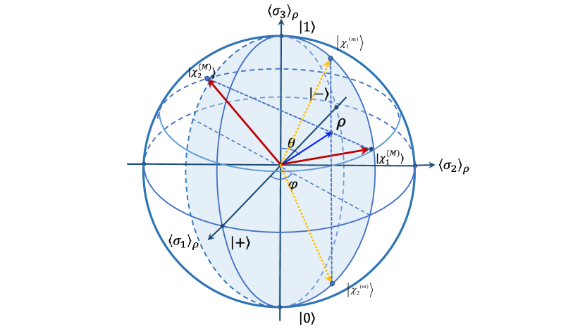
Figure 2: (Color Online) The optimal pure state decompositions of $\rho$ for the convex roof extension $\widehat{V}_{c}(\rho)$ and the concave bottom extension $\widehat{V}_{a}(\rho)$. The pure state decomposition $\left\{p_{k}^{(m)},|\chi_{k}^{(m)}\rangle\right\}_{k=1}^{2}$ (dashed lines) is optimal for the convex roof extension $\widehat{V}_{c}(\rho)$. The pure state decomposition $\left\{p_{k}^{(M)},|\chi_{k}^{(M)}\rangle\right\}_{k=1}^{2}$ (solid lines) is optimal for the concave bottom extension $\widehat{V}_{a}(\rho)$.

III Connections with quantum entanglement

To have an intuitive illustration on the relations between the standard symmetrized variance and the quantum entanglement, let us consider bipartite pure states in Schmidt decomposition form, $|\psi_{AB}\rangle=\sum_{i=0}^{d-1}\lambda_{i}|ii\rangle$ with $\lambda_{i}\geq 0$, $\sum_{i}\lambda_{i}=1$ and local diagonal observable $\bm{A}\otimes\bm{B}=\sum_{i}a_{i}|i\rangle\!\langle i|\otimes\sum_{i}b_{i}|i\rangle\!\langle i|$ acting on $C^{d}\otimes C^{d}$. The variance of the local diagonal observable $\bm{A}\otimes\bm{B}$ in bipartite pure state $|\psi_{AB}\rangle$ is $\operatorname{Var}(|\psi_{AB}\rangle,\bm{A}\otimes\bm{B})=\left\langle\psi_{AB}\left|\bm{A}^{2}\otimes\bm{B}^{2}\right|\psi_{AB}\right\rangle-\left\langle\psi_{AB}\left|\bm{A}\otimes\bm{B}\right|\psi_{AB}\right\rangle^{2}$. Similarly we have the symmetrized variance $\widehat{\operatorname{Var}}(|\psi_{AB}\rangle,\bm{A}\otimes\bm{B})$,

$$\begin{array}[]{rcl}\widehat{\operatorname{Var}}(|\psi_{AB}\rangle,\bm{A}\otimes\bm{B})=\frac{1}{d!}\sum_{\pi\in S_{d}}\operatorname{Var}(\bm{P}_{\pi}\otimes\bm{P}_{\pi}|\psi_{AB}\rangle,\bm{A}\otimes\bm{B}).\end{array}$$ (14)

By direct calculation we have

$$\widehat{\operatorname{Var}}(|\psi_{AB}\rangle,\bm{A}\otimes\bm{B})=\kappa(\bm{A}\bm{B})\left[1-\sum^{d-1}_{i=0}\left\lvert\mspace{1.0mu}\lambda_{i}\mspace{1.0mu}\right\rvert^{4}\right].$$

Then the standard symmetrized variance $\widehat{V}(|\psi_{AB}\rangle)$ is given by

$$\widehat{V}(|\psi_{AB}\rangle) = \frac{1}{\kappa(\bm{A}\bm{B})}\widehat{\operatorname{Var}}(|\psi_{AB}\rangle,\bm{A}\otimes\bm{B})$$

$$= 1-\sum^{d-1}_{i=0}\left\lvert\mspace{1.0mu}\lambda_{i}\mspace{1.0mu}\right\rvert^{4}.$$

It is obvious that $\widehat{V}(|\psi_{AB}\rangle)$ is a real symmetric concave function of the Schmidt vector $(\lambda_{0},\lambda_{1},\cdots,\lambda_{d-1})^{\scriptscriptstyle\mathsf{T}}$. Therefore, $\widehat{V}(|\psi_{AB}\rangle)$ is an entanglement measure for pure state $|\psi_{AB}\rangle$ G. Vidal . Then the convex roof extension of the standard symmetrized variance $\widehat{V}_{c}(\rho_{AB})=\min_{\{p_{k},|\psi^{(k)}_{AB}\rangle\}}\sum_{k}p_{k}\widehat{V}(|\psi^{(k)}_{AB}\rangle)$, where the minimum runs over all possible pure state decompositions of $\rho_{AB}=\sum_{k}p_{k}|\psi^{(k)}_{AB}\rangle\langle\psi^{(k)}_{AB}|$, is an entanglement measure for bipartite quantum states. Recall that the well-known entanglement measure concurrence of a pure state $|\psi_{AB}\rangle$ is defined by $\mathrm{E}(|\psi_{AB}\rangle)=\sqrt{2(1-\operatorname{Tr}\left(\rho_{A}^{2}\right))}$ with $\rho_{A}=Tr_{B}(|\psi_{AB}\rangle\langle\psi_{AB}|)$, and $E(\rho_{AB})=\min_{\{p_{k},|\psi^{(k)}_{AB}\rangle\}}\sum_{k}p_{k}\mathrm{E}(|\psi_{AB}^{(k)}\rangle)$ with the minimum running over all possible pure state decompositions of $\rho_{AB}=\sum_{k}p_{k}|\psi^{(k)}_{AB}\rangle\langle\psi^{(k)}_{AB}|$ W. Wooters ; P. Rungta . By straightforward derivation we find that $\widehat{V}(|\psi_{AB}\rangle)=\frac{1}{2}\mathrm{E}^{2}(|\psi_{AB}\rangle)$ and $\widehat{V}_{c}(\rho_{AB})=\frac{1}{2}\min_{\{p_{k},|\psi^{(k)}_{AB}\rangle\}}\sum_{k}p_{k}\mathrm{E}^{2}(|\psi_{AB}^{(k)}\rangle)$. Equivalently, $E(\rho_{AB})=\min_{\{p_{k},|\psi^{(k)}_{AB}\rangle\}}\sum_{k}p_{k}\sqrt{2\widehat{V}(|\psi_{AB}^{(k)}\rangle)}$, namely, the entanglement measure concurrence can be expressed in terms of the variance.

Since the standard symmetrized variance $\widehat{V}(|\psi_{AB}\rangle)$ is observable-independent, we can choose the projective measurement onto the Schmidt basis of the pure state $|\psi_{AB}\rangle=\sum_{i=0}^{d-1}\lambda_{i}|ii\rangle$, $\Pi^{A}_{i}=|i\rangle\langle i|$ and $\Pi^{B}_{i}=|i\rangle\langle i|$. In this way, we obtain

$$\widehat{V}(|\psi_{AB}\rangle)$$

$$= \frac{1}{d}\sum_{i=0}^{d-1}[\left\langle\psi_{AB}\left|\Pi^{A}_{i}\otimes\Pi^{B}_{i}\right|\psi_{AB}\right\rangle-\left\langle\psi_{AB}\left|\Pi^{A}_{i}\otimes\Pi^{B}_{i}\right|\psi_{AB}\right\rangle^{2}].$$

Therefore, in order to measure the entanglement of a pure state experimentally, one only needs to measure the expectation values $\left\langle\psi_{AB}\left|\Pi^{A}_{i}\otimes\Pi^{B}_{i}\right|\psi_{AB}\right\rangle$ for $i=0,1,\cdots,d-1$.

Different from the uncertainty and coherence, entanglement characterizes the quantum correlations between the subsystems and is basis-independent. Here we have supposed that the pure state $|\psi_{AB}\rangle$ is in Schmidt decomposition form and the observables of the subsystems $A$ and $B$ are diagonal in the Schmidt basis. Then the standard symmetrized variance $\widehat{V}(|\psi_{AB}\rangle)$ as well as the convex roof extension $\widehat{V}_{c}(\rho_{AB})$ are basis independent. They are indeed entanglement measures.

IV Conclusions

In summary, we have proposed the standard symmetrized variance for pure states and extended it to mixed states in three different ways. The first extension quantifies the uncertainty in quantum states. The second convex roof extension quantifies the coherence in quantum states. The third concave bottom extension quantifies the coherence of assistance. These quantities have been estimated in detail. Besides, the standard symmetrized variance also quantifies the entanglement in bipartite systems and gives an experimental way to evaluate the entanglement by measurements. In this way, the quantum uncertainty, coherence and entanglement are closely connected by the standard symmetrized variance.

V Appendices

Appendix A. The proof of Theorem 1.

Proof.

First, Let $\delta_{\pi(i),j}$ be the Kronecker delta symbol defined by $\delta_{\pi(i),j}=1$ if $\pi(i)=j$ and $\delta_{\pi(i),j}=0$ if $\pi(i)\neq j$. We denote $\bm{P}_{\pi}=(\delta_{\pi(i),j})$ the permutation matrix representation of $\pi\in S_{d}$, the set of all possible permutations on the set $\{0,1,\ldots,d-1\}$. Then for any diagonal observable $\bm{A}$ with diagonal entries $a_{i}$, we have the following relations

$$\frac{1}{d!}\sum_{\pi\in S_{d}}a^{2}_{\pi(i)}=\frac{\operatorname{Tr}\left(\bm{A}^{2}\right)}{d}$$ (16)

for any $i$, and

$$\frac{1}{d!}\sum_{\pi\in S_{d}}a_{\pi(i)}a_{\pi(j)}=\frac{[\operatorname{Tr}\left(\bm{A}\right)]^{2}-\operatorname{Tr}\left(\bm{A}^{2}\right)}{d(d-1)}$$ (17)

for any $i\neq j$, where the summation goes over all possible permutations.

Now we are ready to prove Theorem 1. From Eq. (16), we have

$$\widehat{\operatorname{Var}}(|\psi\rangle,\bm{A})$$

$$= \frac{1}{d!}\sum_{\pi\in S_{d}}\left[\left\langle\psi\left|(\bm{P}^{\dagger}_{\pi}\bm{A}\bm{P}_{\pi})^{2}\right|\psi\right\rangle-\left\langle\psi\left|\bm{P}^{\dagger}_{\pi}\bm{A}\bm{P}_{\pi}\right|\psi\right\rangle^{2}\right]$$

$$= \left\langle\psi\left|\frac{1}{d!}\sum_{\pi\in S_{d}}\left(\bm{A}^{\pi}\right)^{2}\right|\psi\right\rangle-\frac{1}{d!}\sum_{\pi\in S_{d}}\left\langle\psi\left|\bm{A}^{\pi}\right|\psi\right\rangle^{2}$$

$$= \frac{\operatorname{Tr}\left(\bm{A}^{2}\right)}{d}-\frac{1}{d!}\sum_{\pi\in S_{d}}\left\langle\psi\left|\bm{A}^{\pi}\right|\psi\right\rangle^{2},$$

where $\bm{A}^{\pi}=\bm{P}^{\dagger}_{\pi}\bm{A}\bm{P}_{\pi}$. Note that $\left\langle\psi\left|\bm{A}^{\pi}\right|\psi\right\rangle^{2}=\sum^{d-1}_{i,j=0}a_{\pi(i)}a_{\pi(j)}r_{i}r_{j}$. We have

$$\frac{1}{d!}\sum_{\pi\in S_{d}}\left\langle\psi\left|\bm{A}^{\pi}\right|\psi\right\rangle^{2}$$

$$= \sum^{d-1}_{i=0}\left(\frac{1}{d!}\sum_{\pi\in S_{d}}a^{2}_{\pi(i)}\right)r^{2}_{i}+\sum^{d-1}_{i\neq j}\left(\frac{1}{d!}\sum_{\pi\in S_{d}}a_{\pi(i)}a_{\pi(j)}\right)r_{i}r_{j}.$$

Using Eqs. (16) and (17), we have further

$$\frac{1}{d!}\sum_{\pi\in S_{d}}\left\langle\psi\left|\bm{A}^{\pi}\right|\psi\right\rangle^{2}$$

$$= \frac{\operatorname{Tr}\left(\bm{A}^{2}\right)}{d}\sum^{d-1}_{i=0}r^{2}_{i}+\frac{[\operatorname{Tr}\left(\bm{A}\right)]^{2}-\operatorname{Tr}\left(\bm{A}^{2}\right)}{d(d-1)}\left(1-\sum^{d-1}_{i=0}r^{2}_{i}\right).$$

Therefore

$$\widehat{\operatorname{Var}}(|\psi\rangle,\bm{A}) = \frac{d\operatorname{Tr}\left(\bm{A}^{2}\right)-[\operatorname{Tr}\left(\bm{A}\right)]^{2}}{d(d-1)}\left[1-\sum^{d-1}_{i=0}r^{2}_{i}\right].$$

This completes the proof. ∎

Appendix B. The proof of Theorem 2.

Proof.

Analogous to the proof of the Theorem 1, one gets

$$\widehat{V}(\rho) = \frac{1}{\kappa(\bm{A})}\frac{1}{d!}\sum_{\pi\in S_{d}}\left[\operatorname{Tr}\left(\bm{A}^{2}\bm{P}_{\pi}\rho\bm{P}^{\dagger}_{\pi}\right)-\left[\operatorname{Tr}\left(\bm{A}\bm{P}_{\pi}\rho\bm{P}^{\dagger}_{\pi}\right)\right]^{2}\right]$$

$$= 1-\sum^{d-1}_{i=0}\rho_{ii}^{2}$$

$$= S_{L}(\Pi(\rho)).$$

This completes the proof. ∎

Appendix C. The proof of the equation

$$\widehat{V}(p_{1}\rho_{1}\oplus p_{2}\rho_{2}\oplus\cdots\oplus p_{n}\rho_{n})$$

$$= p_{1}^{2}\widehat{V}(\rho_{1})+p_{2}^{2}\widehat{V}(\rho_{2})+\cdots+p_{n}^{2}\widehat{V}(\rho_{n})+\sum_{i\neq j}p_{i}p_{j}.$$

Proof.

If $\rho=p_{1}\rho_{1}\oplus p_{2}\rho_{2}\oplus\cdots\oplus p_{n}\rho_{n}$, by Theorem 2, we have

$$\widehat{V}(p_{1}\rho_{1}\oplus p_{2}\rho_{2}\oplus\cdots\oplus p_{n}\rho_{n})$$

$$= 1-Tr(\Pi(\rho))^{2}$$

$$= 1-Tr(\Pi(p_{1}\rho_{1}\oplus p_{2}\rho_{2}\oplus\cdots\oplus p_{n}\rho_{n}))^{2}$$

$$= 1-Tr(\Pi(p_{1}\rho_{1}))^{2}-Tr(\Pi(p_{2}\rho_{2}))^{2}-\cdots-Tr(\Pi(p_{n}\rho_{n}))^{2}$$

$$= [p_{1}^{2}-p_{1}^{2}Tr(\Pi(\rho_{1}))^{2}]+[p_{2}^{2}-p_{2}^{2}Tr(\Pi(\rho_{2}))^{2}]$$

$$+\cdots+[p_{n}^{2}-p_{n}^{2}Tr(\Pi(\rho_{n}))^{2}]+\sum_{i\neq j}p_{i}p_{j}$$

$$= p_{1}^{2}\widehat{V}(\rho_{1})+p_{2}^{2}\widehat{V}(\rho_{2})+\cdots+p_{n}^{2}\widehat{V}(\rho_{n})+\sum_{i\neq j}p_{i}p_{j}.$$

∎

Appendix D. The proof of Theorem 3.

Proof.

For any mixed state $\rho$, by the relation about the minimum average invariance over all pure state decomposition and the quantum Fisher information Yu2013 ; Toth2013 ; S. Braunstein ; G. Toth2017

$$F(\rho,\bm{A})=4\min_{\{p_{k},|\psi_{k}\rangle\}}\sum_{k}p_{k}\operatorname{Var}(|\psi_{k}\rangle,\bm{A}),$$ (18)

we have

$$\min_{\{p_{k},|\psi_{k}\rangle\}}\sum_{k}p_{k}\widehat{\operatorname{Var}}(|\psi_{k}\rangle,\bm{A})$$

$$\geqslant\frac{1}{d!}\sum_{\pi\in S_{d}}\min_{\{p_{k},|\psi_{k}\rangle\}}\sum_{k}p_{k}\operatorname{Var}(\bm{P}_{\pi}|\psi_{k}\rangle,\bm{A})$$

$$=\frac{1}{d!}\sum_{\pi\in S_{d}}\frac{1}{4}F(\bm{P}_{\pi}\rho\bm{P}^{\dagger}_{\pi},\bm{A})$$

$$=\frac{1}{2}\sum_{k,l}\frac{(\lambda_{k}-\lambda_{l})^{2}}{\lambda_{k}+\lambda_{l}}\frac{1}{d!}\sum_{\pi\in S_{d}}|\left\langle\phi_{k}\left|\bm{P}^{\dagger}_{\pi}\bm{A}\bm{P}_{\pi}\right|\phi_{l}\right\rangle|^{2}$$

$$=\frac{1}{2}\sum_{k,l}\frac{(\lambda_{k}-\lambda_{l})^{2}}{\lambda_{k}+\lambda_{l}}\sum_{i,j}\phi^{(k)*}_{i}\phi^{(l)}_{i}\phi^{(l)*}_{j}\phi^{(k)}_{j}\left(\frac{1}{d!}\sum_{\pi\in S_{d}}a_{\pi(i)}a_{\pi(j)}\right).$$

For $i=j$, we have by Eq. (16),

$$\sum_{i}\left\lvert\mspace{1.0mu}\phi^{(k)}_{i}\mspace{1.0mu}\right\rvert^{2}\left\lvert\mspace{1.0mu}\phi^{(l)}_{i}\mspace{1.0mu}\right\rvert^{2}\left[\frac{1}{d!}\sum_{\pi\in S_{d}}a_{\pi(i)}^{2}\right]$$

$$= \frac{\operatorname{Tr}\left(\bm{A}^{2}\right)}{d}\sum_{i}\left\lvert\mspace{1.0mu}\phi^{(k)}_{i}\mspace{1.0mu}\right\rvert^{2}\left\lvert\mspace{1.0mu}\phi^{(l)}_{i}\mspace{1.0mu}\right\rvert^{2}.$$

For $i\neq j$, from Eq. (17) and the orthogonality $\langle\phi_{k}|\phi_{l}\rangle=0$ for $k\neq l$ we have

$$\sum_{i\neq j}\phi^{(k)*}_{i}\phi^{(l)}_{i}\phi^{(l)*}_{j}\phi^{(k)}_{j}\left[\frac{1}{d!}\sum_{\pi\in S_{d}}a_{\pi(i)}a_{\pi(j)}\right]$$

$$= -\frac{[\operatorname{Tr}\left(\bm{A}\right)]^{2}-\operatorname{Tr}\left(\bm{A}^{2}\right)}{d(d-1)}\sum_{i}\left\lvert\mspace{1.0mu}\phi^{(k)}_{i}\mspace{1.0mu}\right\rvert^{2}\left\lvert\mspace{1.0mu}\phi^{(l)}_{i}\mspace{1.0mu}\right\rvert^{2}.$$

Therefore,

$$\min_{\{p_{k},|\psi_{k}\rangle\}}\sum_{k}p_{k}\widehat{\operatorname{Var}}(|\psi_{k}\rangle,\bm{A})$$

$$\geqslant \frac{\kappa(\bm{A})}{2}\sum_{k,l}\frac{(\lambda_{k}-\lambda_{l})^{2}}{\lambda_{k}+\lambda_{l}}\sum_{i}|\phi^{(k)}_{i}|^{2}|\phi^{(l)}_{i}|^{2},$$

which completes the proof. ∎

Appendix E. The proof of Theorem 4.

Proof.

In the permutation group $S_{2}$, it has two permutations: $(1)$ and $(1,2)$. For any qubit mixed state $\rho$, one has $\bm{P}^{\dagger}_{\pi}\sigma_{3}\bm{P}_{\pi}=-\sigma_{3}$ for $\pi=(1,2)$. Utilizing the Eq. (18), we have

$$\min_{\{p_{k},|\psi_{k}\rangle\}}\sum_{k}p_{k}\widehat{\operatorname{Var}}(|\psi_{k}\rangle,\sigma_{3})$$

$$= \frac{1}{2}\min_{\{p_{k},|\psi_{k}\rangle\}}\sum_{k}p_{k}\sum_{\pi\in S_{2}}\operatorname{Var}(\bm{P}_{\pi}|\psi_{k}\rangle,\sigma_{3})$$

$$= \frac{1}{2}\min_{\{p_{k},|\psi_{k}\rangle\}}\sum_{k}p_{k}\sum_{\pi\in S_{2}}\operatorname{Var}(|\psi_{k}\rangle,\bm{P}^{\dagger}_{\pi}\sigma_{3}\bm{P}_{\pi})$$

$$= \min_{\{p_{k},|\psi_{k}\rangle\}}\sum_{k}p_{k}\operatorname{Var}(|\psi_{k}\rangle,\sigma_{3})$$

$$= \frac{1}{4}F(\rho,\sigma_{3})$$

$$= (\lambda_{1}-\lambda_{2})^{2}\left\langle\phi_{1}\left|\sigma_{3}\right|\phi_{2}\right\rangle^{2}.$$

Combining with $\kappa(\sigma_{3})=2$, we get $\widehat{V}_{c}(\rho)=\frac{1}{8}F(\rho,\sigma_{3})=\frac{1}{2}(\lambda_{1}-\lambda_{2})^{2}\left\langle\phi_{1}\left|\sigma_{3}\right|\phi_{2}\right\rangle^{2}$. This completes the proof. ∎

Appendix F. The proof of Theorem 5.

Proof.

In qubit systems, we have $\widehat{V}_{c}(\rho)=\frac{1}{8}F(\rho,\sigma_{3})$ and $\widehat{V}_{a}(\rho)=\widehat{V}(\rho)=\frac{1}{2}\operatorname{Var}(\rho,\sigma_{3})$. For any rank two mixed state $\rho$ and observable $\bm{A}$, one has $\operatorname{Var}(\rho,\bm{A})-F(\rho,\bm{A})=\frac{1}{2}[1-\operatorname{Tr}\left(\rho^{2}\right)](\omega_{1}-\omega_{2})^{2}$ with $\omega_{k}$ the eigenvalues of $\bm{A}$ G. Toth2017 . Therefore, we have

$$\widehat{V}_{a}(\rho)-\widehat{V}_{c}(\rho) = \frac{3}{8}\operatorname{Var}(\rho,\sigma_{3})+\frac{1}{8}[\operatorname{Var}(\rho,\sigma_{3})-F(\rho,\sigma_{3})]$$

$$= \frac{3}{8}[1-\operatorname{Tr}\left(\Pi(\rho)^{2}\right)]+\frac{1}{4}[1-\operatorname{Tr}\left(\rho^{2}\right)].$$

This completes the proof. ∎

References

• (1) W. Heisenberg, Über den anschaulichen Inhalt der quantentheoretischen Kinematik und Mechanik, Zeitschrift für Physik, 43, 172 (1927).
• (2) H.P. Robertson, The Uncertainty Principle, Phys. Rev. 34, 163 (1929).
• (3) L. Maccone, A.K. Pati, Stronger uncertainty relations for all incompatible observables, Phys. Rev. Lett. 113, 260401 (2014).
• (4) S. Friedland, V. Gheorghiu, and G. Gour, Universal Uncertainty Relations, Phys. Rev. Lett. 111, 230401 (2013).
• (5) R. Schwonnek, L. Dammeier, R.F. Werner, State-independent uncertainty relations and entanglement detection in noisy systems, Phys. Rev. Lett. 119, 170404 (2017).
• (6) L. Dammeier, R. Schwonnek, R.F. Werner, Uncertainty relations for angular momentum, New. J. Phys. 17, 093046 (2015).
• (7) L. Zhang, S. Luo, S.M. Fei, and J. Wu, Uncertainty regions of observables and state-independent uncertainty relations, Quantum Inf Process, 20, 357 (2021).
• (8) S. Yu, Quantum Fisher Information as the Convex Roof of Variance, arXiv:1302.5311.
• (9) G. Tóth and D. Petz, Extremal properties of the variance and the quantum Fisher information, Phys. Rev. A87, 032324 (2013).
• (10) S.L. Braunstein and C.M. Caves, Statistical Distance and the Geometry of Quantum States, Phys. Rev. Lett. 72, 3439 (1994).
• (11) G. T$\rm\acute{o}$th, Lower bounds on the quantum Fisher information based on the variance and various types of entropies, arXiv: 1701.07461v5.
• (12) S. Luo, Heisenberg uncertainty relation for mixed states, Phys. Rev. A 72, 042110 (2005).
• (13) G. Tóth and F. Fröwis, Uncertainty relations with the variance and the quantum Fisher information based on convex decompositions of density matrices, Phys. Rev. Research 4, 013075 (2022).
• (14) S.H. Chiew and M. Gessner, Improving sum uncertainty relations with the quantum Fisher information, arXiv: 2109.06900.
• (15) X.M. Lu and X. Wang, Incorporating Heisenberg’s Uncertainty Principle into Quantum Multiparameter Estimation, Phys. Rev. Lett. 126, 120503 (2021).
• (16) H.F. Hofmann and S. Takeuchi, Violation of local uncertainty relations as a signature of entanglement, Phys. Rev. A 68, 032103 (2003).
• (17) O. G$\rm\ddot{u}$hne and G. T$\rm\acute{o}$th, Entanglement detection, Phys. Rep. 474, 1 (2009).
• (18) N. Li and S. Luo, Entanglement detection via quantum Fisher information, Phys. Rev. A 88, 014301 (2013).
• (19) Y. Hong, X, Qi, T. Gao, and F. Yan, Detection of multipartite entanglement via quantum Fisher information, Europhysics Letters, 134 60006 (2021).
• (20) Y. Zhang and S. Luo, Quantum states as observables: Their variance and nonclassicality, Phys. Rev. A 102, 062211 (2020).
• (21) L. Li, Q.W. Wang, S.Q. Shen, and M. Li, Quantum coherence measures based on Fisher information with applications, Phys. Rev. A103, 012401 (2021).
• (22) J. Xu, Quantifying coherence with respect to general measurements via quantum Fisher information, arXiv: 2107.10615.
• (23) S. Du, Z. Bai, and X. Qi, Coherence measures and optimal conversion for coherent states, Quantum Inf. Comput. 15, 1307 (2015).
• (24) H. Zhu, Z. Ma, Z. Cao, S. M. Fei, and V. Vedral, Operational one-to-one mapping between coherence and entanglement measures, Phys. Rev. A 96, 032316 (2017).
• (25) S. Luo, Quantum versus classical uncertainty, Theor. Math. Phys. 143, 681 (2005).
• (26) S. Luo and Y. Sun, Quantum coherence versus quantum uncertainty, Phys. Rev. A 96, 022130 (2017).
• (27) Y. Sun and S. Luo, Coherence as uncertainty, Phys. Rev. A 103, 042423 (2021).
• (28) J. I. de Vicente and A. Streltsov, Genuine quantum coherence, J. Phys. A 50, 045301 (2017).
• (29) X.D. Yu, D.J. Zhang, G.F. Xu, and D.M. Tong, Alternative framework for quantifying coherence, Phys. Rev. A 94, 060302 (2016).
• (30) X.N. Feng and L.F. Wei, Quantifying quantum coherence with quantum Fisher information, Sci. Rep. 7, 15492 (2017).
• (31) H. Kwon, K.C. Tan, S. Choi, and H. Jeong, Comment on “Quantifying quantum coherence with quantum Fisher information”, arXiv: 1711.10110v1.
• (32) E. Chitambar, A. Streltsov, S. Rana, M.N. Bera, G. Adesso, and M. Lewenstein, Assisted Distillation of Quantum Coherence, Phys. Rev. Lett. 116, 070402 (2016).
• (33) M.J. Zhao, T. Ma, and R. Pereira, Average quantum coherence of pure-state decomposition, Phys. Rev. A 103, 042428 (2021).
• (34) W.K. Wootters, Entanglement of Formation of an Arbitrary State of Two Qubits, Phys. Rev. Lett. 80, 2245 (1998).
• (35) P. Rungta, V. Bu$\rm\check{z}$ek, C.M. Caves, M. Hillery, and G.J. Milburn, Universal state inversion and concurrence in arbitrary dimensions, Phys. Rev. A 64, 042315 (2001).
• (36) G. Vidal, Entanglement monotones. J. Mod. Opt. 47, 355 (2000).