Distributed Safe Resource Allocation using Barrier Functions

Abstract

Resource allocation plays a central role in many networked systems such as smart grids, communication networks and urban transportation systems. In these systems, many constraints have physical meaning and having feasible allocation is often vital to avoid system breakdown. Hence, algorithms with asymptotic feasibility guarantees are often insufficient since it is impractical to run algorithms for an infinite number of rounds. This paper proposes a distributed feasible method (DFM) for safe resource allocation based on barrier functions. In DFM, every iterate is feasible and thus safe to implement. We prove that under mild conditions, DFM converges to an arbitrarily small neighbourhood of the optimal solution. Numerical experiments demonstrate the competitive performance of DFM.

, ,

1 Introduction

Resource allocation among cooperative agents in networked systems is a central problem in water distribution networks, urban transportation systems, and power networks. In these systems, an allocation is safe only when it is feasible, and violation of physical constraints may cause system breakdown. Consequently, it is important that resource allocation mechanisms always generate feasible allocations. To make these challenges more concrete, we consider three resource allocation problems from power networks and communications that currently lack distributed solutions.

Economic dispatch [20]: In a smart grid where some users can generate power and some users have demands, the users wish to cooperatively find the optimal power allocations:

$$\underset{x_{i}\in\mathbb{R},i\in\mathcal{V}}{\text{minimize}} \sum_{i\in\mathcal{V}}f_{i}(x)$$ (1)

subject to $$\sum_{i\in\mathcal{V}}x_{i}=c,$$

$$x_{i}\in\mathcal{X}_{i},~{}~{}i\in\mathcal{V}$$

where $x_{i}\in\mathbb{R}$ is the power injection of node $i\in\mathcal{V}$ (negative injection $x_{i}<0$ means that node $i$ consumes power from the grid). The cost function $f_{i}$ is the generation cost or the disutility related to shifting power demands for node $i$, and $c\in\mathbb{R}$ is the power injection not accounted for by the nodes in $\mathcal{V}$. The coupling constraint ensures that the supply meets the demand, which is a hard physical constraint in power systems. The local constraints $\mathcal{X}_{i}$ are important, as they specify hard constraints on devices or user preferences.

Multiple resources [5]: In smart grids, users might get power from different sources, e.g., renewable or coal, with different preference and the goal is to minimize user’s total disutility. To model such scenarios, we need to consider multiple coupling constraints, e.g.,

$$\underset{x_{i}\in\mathbb{R}^{2},i\in\mathcal{V}}{\text{minimize}} \sum_{i\in\mathcal{V}}f_{i}(x_{i}^{\text{renew}},x_{i}^{\text{coal}})$$ (2)

subject to $$\sum_{i\in\mathcal{V}}x_{i}^{\text{renew}}=0,~{}~{}\sum_{i\in\mathcal{V}}x_{i}^{\text{coal}}=0,$$

$$x_{i}\in\mathcal{X}_{i},~{}i\in\mathcal{V}.$$

Here, the local objective functions encode user preferences for different energy sources. This problem is similar to economic dispatch, but is more challenging to solve. In fact, as we will review in Section 1.1, most existing feasible methods can only handle a single coupling constraint.

Rate control in networks [8]: Consider a network with several transmitters where each user $i$ transmits along a single route. The goal is to find the end-to-end transmission rates $x_{i}$ that maximize the total user utility

$$\begin{split}\underset{x_{i}\in\mathbb{R},~{}i\in\mathcal{V}}{\operatorname{maximize}}~{}~{}&~{}\sum_{i\in\mathcal{V}}U_{i}(x_{i})\\ \operatorname{subject~{}to}~{}&~{}\sum_{i\in\mathcal{T}_{\ell}}x_{i}\leq c_{\ell},\quad\forall\ell\in\mathcal{L},\\ &~{}x_{i}\geq 0,~{}\forall i\in\mathcal{V}.\end{split}$$ (3)

Here, $\mathcal{V}$ is the set of transmitters (users), $x_{i}$ and $U_{i}$ are the transmission rate and the utility function of user $i\in\mathcal{V}$, respectively, $\mathcal{L}$ is the set of communication links, and $c_{\ell}$ is the capacity of link $\ell\in\mathcal{L}$. Moreover, $\mathcal{T}_{\ell}$ is the set of transmitters whose data flow is routed across link $\ell$.

1.1 Literature Review

In the past few decades, many distributed algorithms [1, 13, 2, 18, 9, 16, 19, 12, 6, 7, 10, 11] have been proposed to solve resource allocation problems. Most of these methods have only asymptotic feasibility guarantees, i.e., they ensure that the limit of iterates is feasible. This is insufficient because in any practical implementation, only a finite number of iterations can be executed. Moreover, unlike centralized environments, where an infeasible point can be projected onto the feasible region, such projections are rarely implementable in networked systems since the constraints are often global while only local communication between neighbors is allowed.

To solve resource allocation problems in a safe way, a number of distributed feasible methods [16, 19, 12, 6, 7, 10, 11] have been proposed. These methods guarantee feasibility of all iterates. Hence, whenever such an algorithm is stopped, the iterate is safe to implement. Among these methods, [16, 19, 12, 6] guarantee feasibility of all iterates, but do not allow for local constraints. However, as we have shown by the introductory examples above, resource allocation problems in physical systems often have local constraints.

The most closely related works in the literature are [7, 10, 11], which allow for local constraints and yield feasible iterates at every iteration. Among them, [7] addresses problems with one global linear equality constraint while [10, 11] consider problems with one global linear inequality constraint. However, these algorithms have serious limitations. They all assume one-dimensional local decision variables, [7] requires the local constraints to be the set of non-negative real numbers, and [10, 11] rely on star networks. Due to these limitations, none of the approaches in  [7, 10, 11] can solve the three motivating examples in Section 1.

1.2 Contribution

Motivated by the lack of distributed feasible methods for solving resource allocation problems with local constraints on general networks, we propose a class of distributed feasible methods (DFM) based on barrier functions. We also propose a reachability condition, which is necessary for a general class of distributed feasible algorithms including DFM and those in [19, 12, 6, 7] to converge to the optimum from an arbitrary initial allocation. Compared to existing feasible methods [7, 10, 11] that allow for local constraints, DFM can handle a broader range of problems and networks. Specifically, DFM allows for

1. multi-dimensional variables, multiple coupling constraints, and general undirected networks, while [7, 10, 11] only consider scalar variables and one coupling constraints, and [10, 11] rely on star networks.

2. non-convex objective functions, while the objective functions are required to be convex in [7, 10] and strongly convex in [11].

With the above features, DFM can solve all the three motivating examples in Section 1.

A preliminary conference version of this work can be found in [17], which also transforms the problem using barrier functions. However, both the algorithm and the convergence results in [17] are different from this article. In particular, the algorithm in [17] is a random algorithm, it requires nodes to share their local cost function with neighbors which may cause privacy issues, and it is only proved to converge asymptotically in expectation on convex problems. In contrast, DFM is deterministic, has deterministic convergence with non-asymptotic rates, and can solve non-convex problems. In addition, DFM needs no sharing of local cost functions between nodes and avoids the related privacy issues.

Paper Organization and Notation

The outline of this paper is as follows: Section 2 formulates the problem, clarifies the challenges, and transforms the problem using barrier functions. Section 3 develops DFM to solve the transformed problem and Section 4 analyses its convergence properties. Subsequently, Section 5 evaluates the practical performance of DFM in numerical experiments. Finally, Section 6 concludes the paper.

Notation. For any set $\mathcal{S}\subseteq\mathbb{R}^{n}$, $|\mathcal{S}|$ represents its cardinality. We define $\|\cdot\|$ as the $\ell_{2}$ vector norm and $\otimes$ as the Kronecker product. In addition, $\mathbf{0}_{m},\mathbf{1}_{m}$, and $I_{m}$ are the $m$-dimensional all-zero vector, the $m$-dimensional all-one vector, and the $m\times m$ identity matrix, respectively; we ignore their subscripts when the dimension is clear from context. For any $x\in\mathbb{R}^{n}$ and positive semidefinite matrix $W$, we define $\|x\|_{W}=\sqrt{x^{T}Wx}$. A function $f:\mathbb{R}^{d}\rightarrow\mathbb{R}$, it is $L$-smooth if $f$ is differentiable on $\mathbb{R}^{d}$ and its gradient $\nabla f$ is Lipschitz continuous with Lipschitz constant $L$, i.e., $\|\nabla f(x)-\nabla f(y)\|\leq L\|x-y\|$ $\forall x,y\in\mathbb{R}^{d}$; it is $\sigma-$strongly convex for some $\sigma>0$ if $f(y)-f(x)\geq\langle g_{x},y-x\rangle+\frac{\sigma}{2}\|x-y\|^{2}$ for all $x,y\in\mathbb{R}^{d}$ and $g_{x}\in\partial f(x)$. Restrictions on the information exchange among agents will be described by an undirected graph $\mathcal{G}=(\mathcal{V},\mathcal{E})$ with node set $\mathcal{V}$ and edge set $\mathcal{E}$. For each node $i\in\mathcal{V}$, we define $\mathcal{N}_{i}=\{j:\{i,j\}\in\mathcal{E}\}$ as its neighbor set and $\bar{\mathcal{N}}_{i}=\mathcal{N}_{i}\cup\{i\}$.

2 Problem, Challenges, and Solution

2.1 Problem Formulation

Consider a network of $n$ nodes described by an undirected graph $\mathcal{G}=(\mathcal{V},\mathcal{E})$, where $\mathcal{V}=\{1,\ldots,n\}$ is the set of vertices (representing nodes) and $\mathcal{E}\subseteq\mathcal{V}\times\mathcal{V}$ is the set of edges (representing links). Each node $i\in\mathcal{V}$ observes a local constraint set $\mathcal{X}_{i}\subset\mathbb{R}^{d_{i}}$, a local cost function $f_{i}:\mathbb{R}^{d_{i}}\rightarrow\mathbb{R}$, and a local constraint matrix $A_{i}\in\mathbb{R}^{m\times d_{i}}$. The nodes aim at cooperatively finding the optimal resource allocation:

$$\begin{split}\underset{x_{i}\in\mathcal{X}_{i},i\in\mathcal{V}}{\operatorname{minimize}}~{}~{}&\sum_{i\in\mathcal{V}}f_{i}(x_{i})\\ \operatorname{subject~{}to}~{}&\sum_{i\in\mathcal{V}}A_{i}x_{i}=c.\end{split}$$ (4)

Note that (4) also allows for coupling inequality constraints in the form of $\sum_{i\in\mathcal{V}}A_{i}x_{i}\leq c$. These are simply handled by introducing local variables $y_{i}$ and local constraints on the form $A_{i}x_{i}\leq y_{i}$ for all nodes $i\in{\mathcal{V}}$, in combination with the global constraint $\sum_{i\in\mathcal{V}}y_{i}=c$. For example, the coupling constraint in (3) can be re-written as

$$x_{i} \leq y_{i\ell},\quad\forall\ell\in\mathcal{L},\forall i\in\mathcal{T}_{\ell},$$ (5)

$$\sum_{i\in\mathcal{T}_{\ell}}y_{i\ell} =c_{\ell},\quad\;\forall\ell\in\mathcal{L}.$$ (6)

For the theoretical analysis, we impose the following assumptions on problem (4).

Assumption 1.

The following conditions hold:

1. Each $f_{i}$ is $L_{i}$-smooth for some $L_{i}>0$.

2. Each $\mathcal{X}_{i}=\{x\in\mathbb{R}^{d_{i}}:g_{i}^{j}(x)\leq 0,~{}j=1,\ldots,q_{i}\}$ for some convex and $\beta$-smooth functions $g_{i}^{j}:\mathbb{R}^{d_{i}}\rightarrow\mathbb{R}$. Moreover, each $g_{i}^{j}$ is $\beta_{1}$-Lipschitz continuous on $\mathcal{X}_{i}$.

3. There exists $\{\tilde{x}_{i}\}_{i\in\mathcal{V}}$ such that $\sum_{i\in\mathcal{V}}A_{i}\tilde{x}_{i}=c$ and $g_{i}^{j}(\tilde{x}_{i})<0$ for all $i\in\mathcal{V}$ and $j=1,\ldots,q_{i}$.

4. The optimal value $f^{\star}$ of problem (4) is bounded from below, i.e., $f^{\star}>-\infty$.

Assumptions 1(a) and (d) are standard in optimization, especially when each $f_{i}$ is non-convex. Assumptions 1(b)–(c) enable the use of barrier functions for the problem transformation in Section 2.3.2.

2.2 Challenges

Solving (4) with non-asymptotic feasibility guarantee in a distributed way is challenging and primal-dual methods generally can only ensure asymptotic feasibility. Existing distributed primal feasible methods for solving (4) include the weighted gradient method in [7, 19], the multi-step weighted gradient method in [6], and the coordinate-wise weighted gradient method in [12]. However, none of them can handle general $A_{i}$’s or general convex $\mathcal{X}_{i}$’s. Specifically, [7, 19, 6] assume each $A_{i}=I$, [12] requires each $A_{i}$ to be a non-zero scalar, [7] needs each $\mathcal{X}_{i}$ to be the set of non-negative scalars, and [19, 6, 12] do not allow for local constraint sets. In this subsection, we will show by simple examples that a straightforward extension of the methods in [7, 19, 6] to handling general $A_{i}$’s or local constraint sets may fail even if $\mathcal{G}$ is connected. The multi-step weighted gradient method [6] is more complicated and is not analysed here for simplicity.

Extension to handle general $A_{i}$’s: When $A_{i}=1$ for all $i\in{\mathcal{V}}$, the methods in [7, 19, 12] can be described as follows. Start from a feasible solution $\{x_{i}^{0}\}_{i\in\mathcal{V}}$. At each iteration, for an edge set $\mathcal{E}^{k}\subseteq\mathcal{E}$, find $p_{ij}^{k}$ $\forall\{i,j\}\in\mathcal{E}^{k}$ by solving

$$\begin{split}\operatorname{minimize}~{}~{}&~{}f_{i}^{k}(x_{i}^{k}+p_{ji})+f_{j}^{k}(x_{j}^{k}+p_{ij})\\ \operatorname{subject~{}to}~{}&~{}p_{ji}+p_{ij}=0,\end{split}$$ (7)

where $f_{i}^{k}(x_{i})=f_{i}(x_{i}^{k})+\langle\nabla f_{i}(x_{i}^{k}),x_{i}-x_{i}^{k}\rangle+\frac{L_{i}}{2}\|x_{i}-x_{i}^{k}\|^{2}$ is a quadratic surrogate function for $f_{i}$ around iterate $x_{i}^{k}$. The decision variable $p_{ij}$ describes the optimal re-allocation of resources from node $i$ to node $j$ (by the optimality conditions for (7), this quantity is proportional to the difference in the gradients of the loss functions of the nodes at their current iterates). For $\{i,j\}\in\mathcal{E}\setminus\mathcal{E}^{k}$, $p_{ij}^{k}=\mathbf{0}$. Then, the resource allocation is updated as

$$x_{i}^{k+1}=x_{i}^{k}+\sum_{j\in\mathcal{N}_{i}}w_{ij}p_{ij}^{k},~{}\forall i\in\mathcal{V}.$$ (8)

where $w_{ij}=w_{ji}>0$ are scalar weights. In the weighted gradient descent method [7, 19], $\mathcal{E}^{k}=\mathcal{E}$ and in the coordinate-wise weighted gradient method [12], $\mathcal{E}^{k}$ is randomly sampled from $\mathcal{E}$. Note that by (8),

$$\sum_{i\in\mathcal{V}}x_{i}^{k+1}-\sum_{i\in\mathcal{V}}x_{i}^{k}=\!\sum_{\{i,j\}\in\mathcal{E}}\!\!\!w_{ij}(p_{ij}^{k}+p_{ji}^{k})=\mathbf{0}.$$ (9)

Hence, if $\{x_{i}^{0}\}_{i\in{\mathcal{V}}}$ satisfies the coupling constraint, then so will $\{x_{i}^{k}\}_{i\in{\mathcal{V}}}$ for all future iterations $k\geq 0$.

For general $A_{i}$’s, it is natural to find a feasible resource-reallocation by replacing (7) by

$$\begin{split}\operatorname{minimize}~{}~{}&~{}f_{i}^{k}(x_{i}^{k}+p_{ji})+f_{j}^{k}(x_{j}^{k}+p_{ij})\\ \operatorname{subject~{}to}~{}&~{}A_{i}p_{ji}+A_{j}p_{ij}=\mathbf{0}.\end{split}$$ (10)

Using a similar argument as above, the resource updates $p_{ij}$ and $p_{ji}$ ensure that future iterates $\{x_{i}^{k}\}_{i\in\mathcal{V}}$ satisfy the global coupling constraint by (9). However, as the next example shows, this algorithm could fail to converge to the optimum.

Example 1.

Consider the line graph with four nodes:

The problem is

$$\begin{split}\underset{x_{i}\in\mathbb{R},~{}i=1,\ldots,4}{\operatorname{minimize}}~{}&~{}\sum_{i=1}^{4}f_{i}(x_{i})=\frac{1}{2}(x_{i}-\theta_{i})^{2}\\ \operatorname{subject~{}to}~{}&~{}x_{1}+x_{4}=1,\end{split}$$ (11)

where $(\theta_{1},\theta_{2},\theta_{3},\theta_{4})=(1,0,0,1)$. This is an example of (4) without local constraints. For this example, the point $(x_{1}^{\prime},x_{2}^{\prime},x_{3}^{\prime},x_{4}^{\prime})=(0,0,0,1)$ is a fixed point of the update (8) with $p_{ij}^{k}$, $\{i,j\}\in\mathcal{E}^{k}$ computing from (10). To see this, note that by letting $x_{i}^{k}=x_{i}^{\prime}$ $\forall i\in\mathcal{V}$, the solution to (10) is $p_{ij}^{k}=p_{ji}^{k}=\mathbf{0}$ for any $\{i,j\}\in\mathcal{E}$. However, the unique optimal solution of (11) is $(1/2,0,0,1/2)$.

In Section 2.3.1 below, we will analyse the issue in Example 1 and propose a reachability condition to handle it.

Extension to handle general local constraint sets: A straightforward extension of the above method to (4) with general local constraint sets is to add the constraints $x_{i}^{k}+p_{ji}\in\mathcal{X}_{i}$ and $x_{j}^{k}+p_{ij}\in\mathcal{X}_{j}$ to problem (10), leading to

$$\begin{split}\operatorname{minimize}~{}~{}&~{}f_{i}^{k}(x_{i}^{k}+p_{ji})+f_{j}^{k}(x_{j}^{k}+p_{ij})\\ \operatorname{subject~{}to}~{}&~{}A_{i}p_{ji}+A_{j}p_{ij}=\mathbf{0},\\ &~{}x_{i}^{k}+p_{ji}\in\mathcal{X}_{i},~{}x_{j}^{k}+p_{ij}\in\mathcal{X}_{j}.\end{split}$$ (12)

The iterates $p_{ij}^{k}$ $\forall\{i,j\}\in\mathcal{E}^{k}$ are obtained by solving the above problem and the remaining parts are the same as earlier, i.e., $p_{ij}^{k}=p_{ji}^{k}=\mathbf{0}$ for $\{i,j\}\in\mathcal{E}\setminus\mathcal{E}^{k}$ and $\{x_{i}^{k+1}\}_{i\in\mathcal{V}}$ is updated by (8). We additionally require $\sum_{j\in\mathcal{N}_{i}}w_{ij}\leq 1$ for all $i\in\mathcal{V}$. Then, $x_{i}^{k+1}$ is a convex combination of $x_{i}^{k}$ and $x_{i}^{k}+p_{ji}^{k}$, $\forall j\in\mathcal{N}_{i}$, which all belong to $\mathcal{X}_{i}$. Hence, $x_{i}^{k+1}\in\mathcal{X}_{i}$ $\forall i\in\mathcal{V}$. By similar derivation in (9), $\{x_{i}^{k+1}\}_{i\in\mathcal{V}}$ is also feasible to the coupling constraint. Therefore, all iterates are feasible to (4).

Below, we show that even if each $A_{i}=1$ which satisfies the conditions in [7, 19, 12], the above method may not converge to the optimum.

Example 2.

Consider the same graph in Example 1, the same objective function in (11), and the constraints

$$\begin{split}\sum_{i=1}^{4}x_{i}=1,x_{i}\in[0,1],~{}\forall i\in\{1,\ldots,4\}.\end{split}$$

For this example, the point $(x_{1}^{\prime},x_{2}^{\prime},x_{3}^{\prime},x_{4}^{\prime})=(0,0,0,1)$ is a fixed point of the extended method because by letting $x_{i}^{k}=x_{i}^{\prime}$ $\forall i\in\mathcal{V}$, for any $\{i,j\}\in\mathcal{E}$, the solution to (12) is $p_{ij}^{k}=p_{ji}^{k}=\mathbf{0}$. However, the unique optimal solution is $(1/2,0,0,1/2)$.

The failure in Example 2 will be addressed in Section 2.3.2 using barrier functions.

2.3 Solution to the Challenges

2.3.1 Reachability of a general class of feasible methods

This subsection proposes a reachability condition. It enables a general class of distributed feasible methods to explore the whole feasible set, which is often necessary for guaranteeing optimality. The condition is also helpful for understanding and circumventing the failure in Example 1. For convenience, let $\mathbf{x}^{k}=[(x_{1}^{k})^{T},\ldots,(x_{n}^{k})^{T}]^{T}$ for all $k\geq 0$ and $A=[A_{1},\ldots,A_{n}]$.

General update scheme: Start from a feasible iterate $\mathbf{x}^{0}$ of (4). For any $k\geq 0$, update the iterate vector according to

$$\mathbf{x}^{k+1}=\mathbf{x}^{k}+\sum_{i\in\mathcal{V}}\mathbf{u}_{i}^{k},$$ (13)

where $\mathbf{u}_{i}^{k}=[(u_{i1}^{k})^{T},\ldots,(u_{in}^{k})^{T}]^{T}$ and $u_{ij}^{k}\in\mathbb{R}^{d_{j}}$ is the change that node $i$ makes on $x_{j}^{k}$, $j\in\mathcal{V}$. We assume that

$$\mathbf{u}_{i}^{k}\in\mathcal{S}_{i}=\{\mathbf{u}_{i}:u_{ij}=\mathbf{0}~{}\forall j\notin\bar{\mathcal{N}}_{i},~{}\sum_{j\in\bar{\mathcal{N}}_{i}}A_{j}u_{ij}=\mathbf{0}\},$$

i.e., each node can only affect its own iterate and the iterates of its neighbors. When nodes only have information of themselves and their neighbors, this is a natural way to preserve feasibility of the coupling constraint. The extended method in Section 2.2 for handling general $A_{i}$’s and the feasible methods in [7, 19, 6, 12] all belong to this scheme.

Below we introduce the reachability condition. Note that by (13) and $\mathbf{u}_{i}^{k}\in\mathcal{S}_{i}$, $\mathbf{x}^{k+1}-\mathbf{x}^{k}\in\mathcal{S}_{1}+\ldots+\mathcal{S}_{n}$. Moreover, $\mathcal{S}_{i}\subseteq\operatorname{Null}(A)$ for all $i\in\mathcal{V}$. Hence, with the update (13), the optimal solution $\mathbf{x}^{\star}$ is reachable from any $\mathbf{x}^{0}\in\operatorname{Null}(A)$ only if the following assumption holds.

Assumption 2 (Reachability).

It holds that

$$\mathcal{S}_{1}+\ldots+\mathcal{S}_{n}=\operatorname{Null}(A).$$ (14)

This assumption involves both the network $\mathcal{G}$ and the constraint matrix $A$. Under Assumption 2, the update (13) can explore the whole set $\{\mathbf{x}:A\mathbf{x}=c\}$ while preserving feasibility of all iterates to the coupling constraint. However, if Assumption 2 fails to hold, the scheme is unable to reach $\mathbf{x}^{\star}$ from any initial allocation $\mathbf{x}^{0}$ that satisfies $\mathbf{x}^{\star}-\mathbf{x}^{0}\in\operatorname{Null}(A)\setminus(\mathcal{S}_{1}+\ldots+\mathcal{S}_{n})$.

It can be verified that Example 1 fails to satisfy Assumption 2. However, by simply adding the link $\{1,4\}$ to $\mathcal{G}$, Assumption 2 holds. Moreover, by the following Lemma, Assumption 2 is satisfied by the coupling constraint in problems (1)-(2) and the coupling constraint (6), which correspond to the three motivating examples in Section 1.

Lemma 1.

If all the $A_{i}$’s have full row rank and $\mathcal{G}$ is connected, then Assumption 2 holds. Moreover, if we define transmitters who share the same transmission link as neighbors in problem (3), i.e., $\mathcal{E}=\{\{i,j\}:~{}i,j\in\mathcal{T}_{\ell}\text{ for some }\ell\in\mathcal{L}\}$, then (6) satisfies Assumption 2.

Proof.

See Appendix 7.1. ∎

In problems (1)-(2), each $A_{i}=I$ which has full row rank. Then by Lemma 1, Assumption 2 holds when $\mathcal{G}$ is connected.

We also discuss Assumption 2 on the consensus constraint.

Example 3 (consensus constraint).

If $\mathcal{G}$ is connected, then the constraint that every iterate should be in consensus, i.e. $x_{1}=x_{2}=\ldots=x_{n}$, can be rewritten as $\sum_{i=1}^{n}[\mathcal{L}_{\mathcal{G}}]_{i}x_{i}=\mathbf{0}$ where $[\mathcal{L}_{\mathcal{G}}]_{i}$ is the $i$th column of the graph Laplacian $\mathcal{L}_{\mathcal{G}}$ of $\mathcal{G}$. Hence, we can include this consensus constraint in problem (4) by letting each $A_{i}=[\mathcal{L}_{\mathcal{G}}]_{i}$. Assumption 2 holds if and only if $\mathcal{G}$ contains a star network, i.e., if $\bar{\mathcal{N}}_{i}=\mathcal{V}$ for some $i\in\mathcal{V}$. This follows since $\mathcal{S}_{i}=\{\mathbf{0}\}$ if $\bar{\mathcal{N}}_{i}\neq\mathcal{V}$ and $\mathcal{S}_{i}=\operatorname{Null}(A)$ otherwise. Therefore, when using the scheme (13) to ensure every iterates to be consensus, the algorithm can in general converge to the optimum of (4) from any feasible initial point only if $\mathcal{G}$ contains a star network.

2.3.2 Problem Transformation using Barrier Function

As illustrated in Example 2, distributed feasible methods for solving (4) may get stuck in non-optimal points when local constraints are present. To solve this issue, we transform the local constraints in (4) using barrier functions:

$$\begin{split}\underset{x_{i}\in\tilde{\mathcal{X}}_{i},i\in\mathcal{V}}{\operatorname{minimize}}~{}~{}~{}&\sum_{i\in\mathcal{V}}f_{i}(x_{i})+\rho B_{i}(x_{i})\\ \operatorname{subject~{}to}~{}&\sum_{i\in\mathcal{V}}A_{i}x_{i}=c,\end{split}$$ (15)

where each $\tilde{\mathcal{X}}_{i}=\{x_{i}\in\mathbb{R}^{d_{i}}:~{}g_{i}^{j}(x_{i})<0,~{}\forall j=1,\ldots,q_{i}\}$ is the interior of $\mathcal{X}_{i}$ and each $B_{i}(x_{i})=-\sum_{j=1}^{q_{i}}\frac{1}{g_{i}^{j}(x_{i})}$ is the inverse barrier function of the constraints $g_{i}^{j}(x_{i})\leq 0$, $\forall j=1,\ldots,q_{i}$. Problem (15) is an approximation of problem (4) whose approximation error will be analysed in Lemma 4.3 in Section 4. In addition, every feasible solution of problem (15) is also feasible to (4).

For simplicity, we rewrite (15) in the compact form:

$$\begin{split}\underset{\mathbf{x}\in\tilde{\mathcal{X}}}{\operatorname{minimize}}~{}~{}~{}&F(\mathbf{x}):=\sum_{i\in\mathcal{V}}f_{i}(x_{i})+\rho B_{i}(x_{i})\\ \operatorname{subject~{}to}~{}&A\mathbf{x}=c,\end{split}$$ (16)

where $\mathbf{x}=[x_{1}^{T},\ldots,x_{n}^{T}]^{T}$, $\mathcal{\tilde{X}}=\tilde{\mathcal{X}}_{1}\times\ldots\times\tilde{\mathcal{X}}_{n}\subset\mathbb{R}^{N}$ with $N=\sum_{i\in\mathcal{V}}d_{i}$, $f(\mathbf{x})=\sum_{i\in\mathcal{V}}f_{i}(x_{i})$, and $B(\mathbf{x})=\sum_{i\in\mathcal{V}}B_{i}(x_{i})$.

3 Distributed Feasible Method (DFM)

This section develops the DFM algorithm to solve problem (4), based on the problem transformation described in Section 2.3.2. In DFM, each node $i\in\mathcal{V}$ holds a local iterate $x_{i}^{k}\in\mathbb{R}^{d_{i}}$, where $k\geq 0$ represents iteration index. For any $i\in\mathcal{V}$ and $k\geq 0$, we define

$$f_{i}^{k}(x_{i})=f_{i}(x_{i}^{k})+\langle\nabla f_{i}(x_{i}^{k}),x_{i}-x_{i}^{k}\rangle+\frac{L_{i}}{2}\|x_{i}-x_{i}^{k}\|^{2}$$

which is a convex approximation of $f_{i}$ around $x_{i}^{k}$.

The first step of DFM is initialization, in which all the nodes cooperatively set $x_{i}^{0}$ $\forall i\in\mathcal{V}$ such that $\mathbf{x}^{0}=[(x_{1}^{0})^{T},\ldots,(x_{n}^{0})^{T}]^{T}$ is feasible to (16). After the initialization, at each iteration $k\geq 0$, each node $i\in\mathcal{V}$ first solves $\{p_{ij}^{k}\}_{j\in\bar{\mathcal{N}}_{i}}$, which is the optimum of the following problem:

$$\begin{split}\underset{p_{ij}\in\mathbb{R}^{d_{j}},~{}j\in\bar{\mathcal{N}}_{i}}{\operatorname{minimize}}~{}&~{}\sum_{j\in\bar{\mathcal{N}}_{i}}(f_{j}^{k}(x_{j}^{k}+p_{ij})+\rho B_{j}(x_{j}^{k}+p_{ij}))\\ \operatorname{subject~{}to}~{}~{}&~{}\sum_{j\in\bar{\mathcal{N}}_{i}}A_{j}p_{ij}=\mathbf{0},\\ &~{}x_{j}^{k}+p_{ij}\in\tilde{\mathcal{X}}_{j},~{}\forall j\in\bar{\mathcal{N}}_{i},\end{split}$$ (17)

and then updates

$$x_{i}^{k+1}=x_{i}^{k}+\sum_{j\in\bar{\mathcal{N}}_{i}}\eta_{j}p_{ji}^{k},$$ (18)

where

$$\eta_{j}=\frac{1}{\max_{\ell\in\bar{\mathcal{N}}_{j}}|\bar{\mathcal{N}}_{\ell}|}.$$ (19)

Algorithm 1 Distributed Feasible Method (DFM)

1:  Initialization:

2:  All the nodes cooperatively choose a feasible solution $\mathbf{x}^{0}=[(x_{1}^{0})^{T},\ldots,(x_{n}^{0})^{T}]^{T}$ of (16) and agree on $\rho>0$.

3:  Each node $i\in\mathcal{V}$ calculates $\eta_{i}$ by (19) through collecting $|\bar{\mathcal{N}}_{j}|$ from all its neighbors $j\in\mathcal{N}_{i}$.

4:  for $k=0,1,\ldots$ do

5:     for each node $i\in\mathcal{V}$ do

6:        broadcast $\nabla f_{i}(x_{i}^{k})$ and $x_{i}^{k}$ to all neighbors $j\in\mathcal{N}_{i}$.

7:        upon receiving $\nabla f_{j}(x_{j}^{k})$ and $x_{j}^{k}$ for all $j\in\mathcal{N}_{i}$, determine $p_{ij}^{k}$ $\forall j\in\bar{\mathcal{N}}_{i}$ by solving (17).

8:        send each $\eta_{i}p_{ij}^{k}$ to $j\in\mathcal{N}_{i}$.

9:        upon receiving $\eta_{j}p_{ji}^{k}$ $\forall j\in\mathcal{N}_{i}$, compute $x_{i}^{k+1}$ by (18).

10:     end for

11:  end for

A detailed distributed implementation of DFM is given in Algorithm 1. In the initialization, each node $i\in\mathcal{V}$ shares $A_{i}$, $\mathcal{X}_{i}$, and $|\bar{\mathcal{N}}_{i}|$ with its neighbors $j\in\mathcal{N}_{i}$, which will be used to solve (17) and implement (18). Sharing of $A_{j}$ or $|\mathcal{N}_{j}|$ between neighbors is common in algorithms [19, 12] for handling problem (4). In addition, when all the $\mathcal{X}_{j}$’s and $A_{j}$’s are identical, this issue disappears.

At each iteration, the communication cost includes the broadcast of $\nabla f_{i}(x_{i}^{k})$ and $x_{i}^{k}$ to every $j\in\mathcal{N}_{i}$ and the transmissions of $\eta_{i}p_{ij}^{k}$ between neighboring nodes $\{i,j\}\in\mathcal{E}$, and the main computational burden is to solve (17), which can be efficiently addressed by the interior point method [15, Section 19].

DFM can be cast into the general update scheme (13). Moreover, it has a close connection to the weighted gradient method [19] when the local constraint sets are absent.

Remark 1 (Connection with weighted gradient method).

Suppose that $\mathcal{X}_{i}=\mathbb{R}$ and $A_{i}=1$ for all $i\in\mathcal{V}$. Then, by letting $L_{i}=L$ $\forall i\in\mathcal{V}$, DFM (17)–(18) becomes the weighted gradient descent method:

$$\mathbf{x}^{k+1}=\mathbf{x}^{k}-\frac{1}{L}H\nabla f(\mathbf{x}^{k}),$$ (20)

where $H=\sum_{i\in\mathcal{V}}\eta_{i}H^{i}$ with $H^{i}=(h_{j\ell}^{i})_{n\times n}$ defined as

$$h_{j\ell}^{i}=\begin{cases}1-\frac{1}{|\bar{\mathcal{N}}_{i}|},&\text{if }j=\ell,\\ -\frac{1}{|\bar{\mathcal{N}}_{i}|},&\text{if }j,\ell\in\bar{\mathcal{N}}_{i}\text{ and }j\neq\ell,\\ 0,&\text{otherwise}.\end{cases}$$

The update (20) takes the same form compared to the typical weighted gradient method [19] which solves the same problem, but has a different weight matrix $H$.

4 Convergence Analysis

This section derives convergence results for DFM. To this end, we first introduce the KKT condition for problem (16), which is necessary for local optimality. A point $\mathbf{x}^{\prime}\in\mathbb{R}^{N}$ satisfies the KKT condition of problem (16) if

1. $\mathbf{x}^{\prime}$ is feasible to problem (16).

2. There exists $v\in\mathbb{R}^{m}$ such that

   $$-\nabla F(\mathbf{x}^{\prime})-A^{T}v\in\mathcal{N}_{\tilde{\mathcal{X}}}(\mathbf{x}^{\prime}),$$ (21)

   where $\mathcal{N}_{\tilde{\mathcal{X}}}(\mathbf{x}^{\prime})$ is the normal cone of $\tilde{\mathcal{X}}$ at $\mathbf{x}^{\prime}$.

Because $\tilde{\mathcal{X}}$ is open, $\mathcal{N}_{\tilde{\mathcal{X}}}(\mathbf{x}^{\prime})=\{\mathbf{0}\}$ for all $\mathbf{x}^{\prime}\in\tilde{\mathcal{X}}$. Thus, the existence of $v\in\mathbb{R}^{m}$ satisfying (21) is equivalent to

$$\nabla F(\mathbf{x}^{\prime})\in\operatorname{Range}(A^{T}).$$

For every $i\in{\mathcal{V}}$, let $P_{i}\in\mathbb{R}^{N\times N}$ be the projection matrix of $\mathcal{S}_{i}$ and define $W=\sum_{i\in\mathcal{V}}\eta_{i}P_{i}$. Under Assumption 2, $\operatorname{Null}(W)=\operatorname{Range}(A^{T})$ and $\mathbf{x}^{\prime}$ is a KKT point of (16) iff $\mathbf{x}^{\prime}$ is feasible and $W\nabla F(\mathbf{x}^{\prime})=\mathbf{0}$. Because $W$ is positive semi-definite, $W\nabla F(\mathbf{x}^{\prime})=\mathbf{0}$ is equivalent to $\|\nabla F(\mathbf{x}^{\prime})\|_{W}=0$.

Let $\mathbf{x}^{k}=[(x_{1}^{k})^{T},\ldots,(x_{n}^{k})^{T}]^{T}$ for all $k\geq 0$, where $x_{i}^{k}$ $\forall i\in\mathcal{V}$ are generated by Algorithm 1.

Theorem 4.1.

Suppose that Assumptions 1–2 hold. Then, $\mathbf{x}^{k}$ $\forall k\geq 0$ are feasible to problems (16) and (4), and

$$\sum_{k=0}^{\infty}\|\nabla F(\mathbf{x}^{k})\|_{W}^{2}\leq 2(\rho L_{B}+L)(F(\mathbf{x}^{0})-f^{\star}),$$ (22)

where $L=\max_{i\in\mathcal{V}}L_{i}$ and $L_{B}=(4\beta_{1}^{2}((F(\mathbf{x}^{0})-f^{\star})/\rho)^{3}+2\beta((F(\mathbf{x}^{0})-f^{\star})/\rho)^{2})\max_{i\in\mathcal{V}}q_{i}$. In addition,

1. if each $f_{i}$ is convex and the set $\mathcal{C}:=\{\mathbf{x}:\mathbf{x}\text{ is feasible to }\eqref{eq:compactprob}\text{ and }F(\mathbf{x})\leq F(\mathbf{x}^{0})\}$ is compact,

   $$F(\mathbf{x}^{k})-F^{\star}\leq\frac{2(L\!+\!\rho L_{B})R^{2}}{k\lambda_{W}},$$ (23)

   where $F^{\star}$ is the optimal value of problem (16), $R$ is the diameter of $\mathcal{C}$, and $\lambda_{W}$ is the smallest nonzero eigenvalue of $W$.

2. if each $f_{i}$ is $\sigma$-strongly convex for some $\sigma>0$,

   $$\begin{split}&F(\mathbf{x}^{k})-F^{\star}\leq\left(1\!-\!\frac{\sigma\lambda_{W}}{L\!+\!\rho L_{B}}\right)^{k}(F(\mathbf{x}^{0})-F^{\star}).\end{split}$$

Proof 4.2.

See Appendix 7.2.

In Theorem 4.1, (22) implies $\lim_{k\rightarrow+\infty}\|\nabla F(\mathbf{x}^{k})\|_{W}^{2}=0$. In addition, according to [4, Lemma 1], (22) also yields $\min_{0\leq t\leq k}\|\nabla F(\mathbf{x}^{t})\|_{W}^{2}=o(1/k)$.

Below, we investigate the optimality gap between problems (4) and (16), provided that all $f_{i}$’s are convex. Specifically, we study the range of $\rho$ for guaranteeing certain accuracy.

Lemma 4.3.

Suppose that Assumptions 1–2 hold and $f_{i}$ $\forall i\in\mathcal{V}$ are convex. Let $\tilde{\mathbf{x}}^{\star}$ be an optimal solution of (16) and $\underline{f}\leq f^{\star}$. For any $\epsilon>0$, $f(\tilde{\mathbf{x}}^{\star})-f^{\star}\leq\epsilon$ if

$$0<\rho\leq\begin{cases}\frac{\epsilon}{2B(\mathbf{x}^{\prime})},&f(\mathbf{x}^{\prime})-\underline{f}\leq\epsilon/2\\ \frac{\epsilon^{2}}{4(f(\mathbf{x}^{\prime})-\underline{f})B(\mathbf{x}^{\prime})},&\text{otherwise}\end{cases}$$ (24)

for some feasible solution $\mathbf{x}^{\prime}$ of (16).

Proof 4.4.

See Appendix 7.3.

By Lemma 4.3, DFM can converge to arbitrarily small error bound of the optimal value. If some $\underline{f}\leq f^{\star}$ is known, (24) can be determined in a distributed way. For example, set $\mathbf{x}^{\prime}=\mathbf{x}^{0}$ and let each node $i$ calculate $f_{i}(x_{i}^{0})$, $B_{i}(x_{i}^{0})$. Then, by adding all the $f_{i}(x_{i}^{0})$ and $B_{i}(x_{i}^{0})$ by distributed sum protocols (e.g., [3]), the quantities $f(\mathbf{x}^{0})$ and $B(\mathbf{x}^{0})$ are obtained by all the nodes, so the range of $\rho$ in (24) is known.

Corollary 4.5.

Suppose that Assumptions 1–2 hold. For any $0<\epsilon<2(f(\mathbf{x}^{0})-f^{\star})$, set $\rho=\frac{\epsilon^{2}}{4(f(\mathbf{x}^{0})-\underline{f})B(\mathbf{x}^{0})}$ and let $k_{\epsilon}$ be the smallest $k\geq 0$ satisfying $f(\mathbf{x}^{k})-f^{\star}\leq 2\epsilon$. Then,

1. Convex: if each $f_{i}$ is convex and $\mathcal{C}$ defined in Theorem 4.1 is compact, then $k_{\epsilon}=O(\frac{1}{\epsilon^{5}\lambda_{W}})$.

2. Strongly convex: if each $f_{i}$ is $\sigma$-strongly convex for some $\sigma>0$, then $k_{\epsilon}=O(\frac{1}{\sigma\lambda_{W}\epsilon^{4}}\ln\frac{1}{\epsilon})$.

Proof 4.6.

Note that $\rho=O(\epsilon^{2})$ and $\rho L_{B}=O(\epsilon^{-4})$, where $L_{B}=O(1/\rho^{3})$ is defined in Theorem 4.1. Then, combining Theorem 4.1 and Lemma 4.3 yields the result.

In Corollary 4.5, we only show the effect of important factors. The Lipschitz constant $L$ is usually small compared to $\rho L_{B}=O(\epsilon^{-4})$ and is therefore ignored. The slow convergence rates in Corollary 4.5 are caused by the use of barrier functions for transforming the difficult problem (4). However, the practical performance of DFM is much better than this worst-case bound, as will be shown in Section 5.

5 Numerical Experiment

To verify the theoretical results in Section 4 and demonstrate the practical performance of DFM, we evaluate DFM against alternative methods on the motivating examples in Section 1. The experimental settings are detailed below.

Experiment I (Economic Dispatch): We consider problem (1) and draw both problem data and communication network from the IEEE-118 bus system [21], where $f_{i}$ is a quadratic function, $\mathcal{X}_{i}:=[\ell_{i},u_{i}]\subset\mathbb{R}$ is a closed interval, and the number of power generators is $n=54$. In addition to generators, the IEEE-118 bus system also includes several non-generators. The generators and non-generators form an undirected, connected communication graph $\mathcal{G}^{\prime}$. To form the communication network ${\mathcal{G}}$ for the generators, we define two generators $i,j$ to be neighbors in $\mathcal{G}$ if there exists a path in $\mathcal{G}^{\prime}$ between $i,j$ which does not include any other generators.

Experiment II (Multiple Resources): We consider problem (2) and draw both problem data and communication network from the IEEE-118 bus system. We let each power generator be a renewable or a coal power generator with equal probability. We treat both generators and non-generators as users and set $n=118$. The user disutility function is $f_{i}(x_{i}^{\text{renew}},x_{i}^{\text{coal}})=\alpha_{i}(x_{i}^{\text{renew}}+x_{i}^{\text{coal}}-D_{i})^{2}+\beta_{i}(x_{i}^{\text{coal}})^{2}$, where $x_{i}^{\text{renew}}$ and $x_{i}^{\text{coal}}$ are renewable and coal power consumption of node $i$, respectively, $D_{i}$ is the power demand of node $i$, $\alpha_{i}>0$ is a parameter indicating the discomfort of user $i$ for changing its demand, and $\beta_{i}>0$ is a parameter capturing the disapproval of user $i$ of using non-renewable energy. We set $\mathcal{X}_{i}=\{x_{i}=(x_{i}^{\text{renew}},x_{i}^{\text{coal}})^{T}:x_{i}\geq\tilde{\ell}_{i}\}$, where $\tilde{\ell}_{i}=(-u_{i},0)^{T}$ if $i$ is a renewable power generator and $\tilde{\ell}_{i}=(0,-u_{i})^{T}$ if $i$ is a coal power generator, where $u_{i}$ is the same as in Experiment I, and $\tilde{\ell}_{i}=(0,0)^{T}$ if $i$ is a non-generator. The communication graph is $\mathcal{G}^{\prime}$ in Experiment I.

Experiment III (Rate Control): We consider problem (3) where the network of routers and the capacity of each link are shown in Fig. 1. Each source $S_{i}$ sends data to $D_{i}$ via some links and routers. We treat source nodes whose routing paths include common links, i.e. $\{S_{1},S_{2}\}$, $\{S_{2},S_{3}\}$, and $\{S_{3},S_{4}\}$, as neighbors in the communication graph. We set each $U_{i}$ in problem (3) as a sigmoidal utility function $U_{i}(x_{i})=\frac{p_{i}}{1+e^{-a_{i}(x_{i}-b_{i})}}+q_{i}$ for some randomly generated $a_{i},b_{i},p_{i}>0$ and choose $q_{i}\in\mathbb{R}$ be such that $U_{i}(0)=0$. Although these utility functions are not concave, they have Lipschitz-continuous gradients and satisfy Assumption 1.

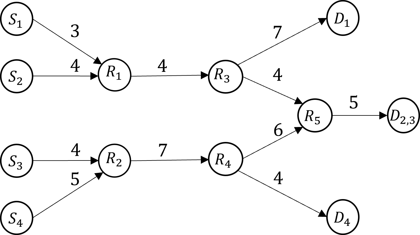
Figure 1: Routing network in Experiment III

(a) DFM

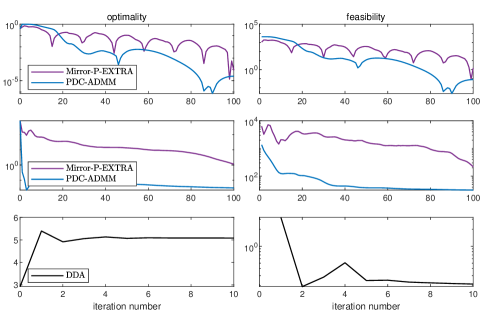
(b) Non-feasible methods

Figure 2: Convergence of methods in Experiment I-III (Optimality represents objective error in Experiment I-II and objective value in Experiment III where the optimal value is unknown due to non-concavity of (3). Feasibility means feasibility error in all experiments).

As detailed in Section 1.1, we have not found distributed feasible methods that can solve any of the three experiments. Hence, we consider non-feasible distributed methods Mirror-P-EXTRA [13] and PDC-ADMM [2] in Experiment I-II and DDA [9] in Experiment III. These methods cannot guarantee feasibility of iterates. For fair comparison, we choose the same initial primal iterate for all methods and tune all parameters within their theoretically justified ranges.

We display the convergence in all the three experiments in Fig. 2, including DFM in Fig. 2(a) and alternative non-feasible methods in Fig. 2(b). The feasibility error of DFM is always $0$ and is thus ignored. Since the initial iterate is feasible, we plot the feasibility error starting from iteration $1$. In Fig. 2, optimality represents the relative objective error $|(f(\mathbf{x}^{k})-f^{\star})/f^{\star}|$ in Experiment I-II and objective value of the maximization problem (3) in Experiment III. Since the sigmoidal function is non-concave, the optimal value of problem (3) is unknown. Moreover, since the local constraints are satisfied by all the simulated methods, we set $|\sum_{i=1}^{n}x_{i}^{k}-c|$, $\|\sum_{i=1}^{n}x_{i}^{k}\|$, and $\sqrt{\sum_{\ell\in\mathcal{E}}(\max(0,\sum_{i\in\mathcal{T}_{\ell}}x_{i}-c_{\ell}))^{2}}$ as the feasibility error in Experiments I-III, respectively.

From Fig. 2, we observe that the objective value of DFM converges quickly in all the experiments even compared with non-feasible methods, which demonstrates the competitive performance of DFM. Although in Experiment II, the objective value of PDC-ADMM converges faster than that of DFM, all non-feasible methods require a large number of iterations to reach small feasibility error. The experiment results also validate Theorem 4.1, i.e., all iterates generated by DFM are feasible to (4) and converge under mild conditions. Moreover, from Figure 2(a), we can see that smaller $\rho$ usually leads to higher accuracy.

6 Conclusion

Our ability to allocate resources in a safe and efficient manner is critical to the operation of many physical network systems. We have proposed a distributed feasible method (DFM) to solve resource allocation problems while guaranteeing that all iterates are feasible and thus safe to implement. DFM is designed based on barrier functions and can handle more general problems (multiple coupling constraints, multi-dimensional variables, and non-convex objective functions) and network topologies than the previous state-of-the-art.

7 Appendix

7.1 Proof of Lemma 1

It’s straightforward to see the left-hand side of (14) is a subset of $\operatorname{Null}(A)$ because $\mathcal{S}_{i}\subseteq\operatorname{Null}(A)$ for all $i\in\mathcal{V}$. Hence, to show (14), we only need to prove

$$\operatorname{Null}(A)\subseteq\mathcal{S}_{1}+\ldots+\mathcal{S}_{n}.$$ (25)

First, we suppose that all the $A_{i}$’s have full row rank and prove (25) by showing that for any $\mathbf{p}\in\operatorname{Null}(A)$, there exist $\mathbf{q}_{i}\in\mathcal{S}_{i}$ $\forall i\in\mathcal{V}$ such that $\sum_{i\in\mathcal{V}}\mathbf{q}_{i}=\mathbf{p}$. Let $p_{i}\in\mathbb{R}^{d_{i}}$ be the $i$th block of $\mathbf{p}$ and decompose each $p_{i}=u_{i}+v_{i}$, where $u_{i}\in\operatorname{Range}(A_{i}^{T})$ and $v_{i}\in\operatorname{Null}(A_{i})$. Let $y_{i}=A_{i}u_{i}$ for all $i\in\mathcal{V}$ and $\mathbf{y}=[(y_{1})^{T},\ldots,(y_{n})^{T}]^{T}$. We have

$$\sum_{i\in\mathcal{V}}y_{i}=\sum_{i\in\mathcal{V}}A_{i}u_{i}=\sum_{i\in\mathcal{V}}A_{i}p_{i}=A\mathbf{p}=\mathbf{0}.$$ (26)

Let $\mathcal{L}_{\mathcal{G}}$ be the graph Laplacian of $\mathcal{G}$. By (26) and the connectivity of $\mathcal{G}$, we have $\mathbf{y}\in\operatorname{Range}(\mathcal{L}_{\mathcal{G}}\otimes I_{m})$, i.e., there exists $\mathbf{z}$ satisfying

$$\mathbf{y}=(\mathcal{L}_{\mathcal{G}}\otimes I_{m})\mathbf{z}.$$

Let $[\mathbf{q}_{i}]_{j}\in\mathbb{R}^{d_{j}},z_{j}\in\mathbb{R}^{m}$ denote the $j$th block of $\mathbf{q}_{i}$ and $\mathbf{z}$, respectively. We construct the following $\mathbf{q}_{i}$:

$$[\mathbf{q}_{i}]_{j}=\begin{cases}A_{i}^{\dagger}[\mathcal{L}_{\mathcal{G}}]_{ii}z_{i}+v_{i},&i=j,\\ A_{j}^{\dagger}[\mathcal{L}_{\mathcal{G}}]_{ji}z_{i},&\text{otherwise},\end{cases}$$

where $A_{j}^{\dagger}=A_{j}^{T}(A_{j}A_{j}^{T})^{-1}$ is the Moore-Penrose inverse of $A_{j}$. Because $[\mathcal{L}_{\mathcal{G}}]_{ji}=0$ for all $j\in\mathcal{V}\setminus\bar{\mathcal{N}}_{i}$, $A_{j}A_{j}^{\dagger}=I$, and $\sum_{j\in\bar{\mathcal{N}}_{i}}[\mathcal{L}_{\mathcal{G}}]_{ji}=0$, we have

$$\mathbf{q}_{i}\in\mathcal{S}_{i},~{}\forall i\in\mathcal{V}.$$ (27)

To see $\sum_{i\in\mathcal{V}}\mathbf{q}_{i}=\mathbf{p}$, note that for each $j\in\mathcal{V}$,

$$\sum_{i\in\mathcal{V}}[\mathbf{q}_{i}]_{j}=v_{j}+A_{j}^{\dagger}\sum_{i\in\bar{\mathcal{N}}_{j}}[\mathcal{L}_{\mathcal{G}}]_{ji}z_{i}=v_{j}+A_{j}^{\dagger}y_{j}=v_{j}+u_{j}=p_{j},$$

where $A_{j}^{\dagger}y_{j}=u_{j}$ because $y_{j}=A_{j}u_{j}$ and $u_{j}\in\operatorname{Range}(A_{j}^{T})$. Summarizing all the above gives (25).

Next, we prove that (6) satisfies (14). Suppose $\mathbf{p}=\{p_{i\ell}\}_{\ell\in\mathcal{L},i\in\mathcal{T}_{\ell}}$ is an arbitrary vector in $\operatorname{Null}(A)$. For any $\tilde{\ell}\in\mathcal{L}$, let $\mathbf{q}^{\tilde{\ell}}=\{q_{i\ell}^{\tilde{\ell}}\}_{\ell\in\mathcal{L},i\in\mathcal{T}_{\ell}}$ be such that

$$q_{i\ell}^{\tilde{\ell}}=\begin{cases}p_{i\ell},&\ell=\tilde{\ell},\\ 0,&\text{otherwise}.\end{cases}$$

Then, $\mathbf{p}=\sum_{\tilde{\ell}\in\mathcal{L}}\mathbf{q}^{\tilde{\ell}}$. Moreover, by the definition of $\mathcal{S}_{i}$, $\mathbf{q}^{\tilde{\ell}}\in\mathcal{S}_{i}$ for all $i\in\mathcal{T}_{\tilde{\ell}}$. Hence, $\mathbf{p}\in\mathcal{S}_{1}+\ldots+\mathcal{S}_{n}$ and (25) holds. Completes the proof.

7.2 Proof of Theorem 4.1

7.2.1 Feasibility

We prove this by induction. Suppose that $\mathbf{x}^{k}$ is feasible to (16) for some $k\geq 0$, which holds naturally at $k=0$. Below, we show that $\mathbf{x}^{k+1}$ is feasible to (16).

By (18),

$$x_{i}^{k+1}=(1-\sum_{j\in\bar{\mathcal{N}}_{i}}\eta_{j})x_{i}^{k}+\sum_{j\in\bar{\mathcal{N}}_{i}}\eta_{j}(x_{i}^{k}+p_{ji}^{k}),$$ (28)

which, together with the feasibility of $\mathbf{x}^{k}$ to problem (16) and $\{p_{ij}^{k}\}_{j\in\bar{\mathcal{N}}_{i}}$ to problem (17), ensures

$$x_{i}^{k},x_{i}^{k}+p_{ji}^{k}\in\tilde{\mathcal{X}}_{i},~{}\forall i\in\mathcal{V},\forall j\in\bar{\mathcal{N}}_{i},$$ (29)

$$\sum_{i\in\mathcal{V}}A_{i}x_{i}^{k+1}=\sum_{i\in\mathcal{V}}A_{i}(x_{i}^{k}+\sum_{j\in\bar{\mathcal{N}}_{i}}\eta_{j}p_{ji}^{k})$$

$$= \sum_{i\in\mathcal{V}}A_{i}x_{i}^{k}+\sum_{i\in\mathcal{V}}\eta_{i}\sum_{j\in\bar{\mathcal{N}}_{i}}A_{j}p_{ij}^{k}=c.$$ (30)

Because $\eta_{j}=\frac{1}{\max_{\ell\in\bar{\mathcal{N}}_{j}}|\bar{\mathcal{N}}_{\ell}|}\leq\frac{1}{|\bar{\mathcal{N}}_{i}|}$ for any $j\in\bar{\mathcal{N}}_{i}$, we have $1-\sum_{j\in\bar{\mathcal{N}}_{i}}\eta_{j}\geq 0$. Then from (28), (29), and the convexity of $\tilde{\mathcal{X}}_{i}$, we have $x_{i}^{k+1}\in\tilde{\mathcal{X}}_{i}$, which, together with (30), yields the feasibility of $\mathbf{x}^{k+1}$ to problem (16).

Concluding all the above, all $\mathbf{x}^{k}$’s are feasible to (16). Since all feasible solution of (16) is feasible to (4), all $\mathbf{x}^{k}$’s are feasible to (4).

7.2.2 Non-convex case

The proof consists of three parts. We first prove

$$F(\mathbf{x}^{k})\leq F(\mathbf{x}^{0}),~{}\forall k\geq 0.$$ (31)

Next, we show that although each barrier function $B_{i}$ is not globally smooth, it is locally smooth. We derive the following using (31): For all $i\in\mathcal{V}$ and $j\in\bar{\mathcal{N}}_{i}$,

$$\begin{split}&B_{i}(x_{i}^{k})-B_{i}(x_{i}^{k}+p_{ji}^{k})-\langle\nabla B_{i}(x_{i}^{k}+p_{ji}^{k}),-p_{ji}^{k}\rangle\\ \geq&\frac{\|\nabla B_{i}(x_{i}^{k})-\nabla B_{i}(x_{i}^{k}+p_{ji}^{k})\|^{2}}{2L_{B}}.\end{split}$$ (32)

Finally, we use (32) to show the result.

Define $F_{i}(x_{i})=f_{i}(x_{i})+\rho B_{i}(x_{i})$ and $B_{i}^{j}(x_{i})=\frac{1}{-g_{i}^{j}(x_{i})}$.

Part 1: proof of (31). Define $\phi_{i}^{k}(x_{i})=f_{i}^{k}(x_{i})+\rho B_{i}(x_{i})$ for each $i\in\mathcal{V}$ and $k\geq 0$. By the $L_{i}$-smoothness of each $f_{i}$, $f_{i}^{k}(x_{i})\geq f_{i}(x_{i})$ so that

$$F_{i}(x_{i})\leq\phi_{i}^{k}(x_{i}),\quad\forall x_{i}\in\mathbb{R}^{d_{i}}.$$ (33)

By (33), the convexity of $\phi_{i}^{k}$, (28), and $\sum_{j\in\bar{\mathcal{N}}_{i}}\eta_{j}\leq 1$,

$$\begin{split}&F(\mathbf{x}^{k+1})\leq\sum_{i\in\mathcal{V}}\phi_{i}^{k}(x_{i}^{k+1})\\ \leq&\sum_{i\in\mathcal{V}}[(1-\!\!\sum_{j\in\bar{\mathcal{N}}_{i}}\eta_{j})\phi_{i}^{k}(x_{i}^{k})\!+\!\sum_{j\in\bar{\mathcal{N}}_{i}}\eta_{j}\phi_{i}^{k}(x_{i}^{k}\!+\!p_{ji}^{k})].\end{split}$$ (34)

Since $\{p_{ij}^{k}\}_{j\in\bar{\mathcal{N}}_{i}}$ is optimal to (17),

$$\sum_{j\in\bar{\mathcal{N}}_{i}}\phi_{j}^{k}(x_{j}^{k}+p_{ij}^{k})\leq\sum_{j\in\bar{\mathcal{N}}_{i}}\phi_{j}^{k}(x_{j}^{k}),$$ (35)

and therefore

$$\begin{split}&\sum_{i\in\mathcal{V}}\sum_{j\in\bar{\mathcal{N}}_{i}}\eta_{j}\phi_{i}^{k}(x_{i}^{k}+p_{ji}^{k})=\sum_{i\in\mathcal{V}}\eta_{i}\sum_{j\in\bar{\mathcal{N}}_{i}}\phi_{j}^{k}(x_{j}^{k}+p_{ij}^{k})\\ &\leq\sum_{i\in\mathcal{V}}\eta_{i}\sum_{j\in\bar{\mathcal{N}}_{i}}\phi_{j}^{k}(x_{j}^{k})=\sum_{i\in\mathcal{V}}\Big{(}\sum_{j\in\bar{\mathcal{N}}_{i}}\eta_{j}\Big{)}\phi_{i}^{k}(x_{i}^{k}).\end{split}$$

Substituting the above equation into (34) and using $F_{i}(x_{i}^{k})=\phi_{i}^{k}(x_{i}^{k})$ $\forall i\in\mathcal{V}$ yields $F(\mathbf{x}^{k+1})\leq\sum_{i\in\mathcal{V}}\phi_{i}^{k}(x_{i}^{k})=F(\mathbf{x}^{k})$ for all $k\geq 0$, which further implies (31).

Part 2: proof of (32). The proof starts from the local smoothness property of $B_{i}^{j}$.

Lemma 7.7.

Suppose that $g_{i}^{j}$, $i\in\mathcal{V}$, $j\in\{1,\ldots,q_{i}\}$ satisfies Assumption 1(b). For any $\mathcal{M}>0$ and $x_{i},y_{i}\in\tilde{\mathcal{X}}_{i}$, if $B_{i}^{j}(x_{i})\leq\mathcal{M}$ and $B_{i}^{j}(y_{i})\leq\mathcal{M}$, then

$$\begin{split}&B_{i}^{j}(y_{i})-B_{i}^{j}(x_{i})-\langle\nabla B_{i}^{j}(x_{i}),y_{i}-x_{i}\rangle\\ \geq&\frac{1}{8\beta_{1}^{2}\mathcal{M}^{3}+4\beta\mathcal{M}^{2}}\|\nabla B_{i}^{j}(y_{i})-\nabla B_{i}^{j}(x_{i})\|^{2}.\end{split}$$ (36)

Proof 7.8.

Define $u=\big{|}\frac{1}{(g_{i}^{j}(y_{i}))^{2}}-\frac{1}{(g_{i}^{j}(x_{i}))^{2}}\big{|}$, $v=\|\nabla g_{i}^{j}(y_{i})-\nabla g_{i}^{j}(x_{i})\|$, and $\bar{g}=\max(|g_{i}^{j}(x_{i})|,|g_{i}^{j}(y_{i})|)$. Also define $\Delta=B_{i}^{j}(y_{i})-B_{i}^{j}(x_{i})-\langle\nabla B_{i}^{j}(x_{i}),y_{i}-x_{i}\rangle$. To derive (36), we first bound $\|\nabla B_{i}^{j}(x_{i})-\nabla B_{i}^{j}(y_{i})\|^{2}$ by $u,v$ and then bound $u,v$ by $\Delta$.

Note that for any $c_{1}>c_{2}>0$ and $z_{1},z_{2}\in\mathbb{R}^{d}$,

$$\begin{split}\Big{\|}\frac{z_{1}}{c_{1}}-\frac{z_{2}}{c_{2}}\Big{\|}&=\Big{\|}\frac{z_{1}-z_{2}}{c_{1}}+\left(\frac{1}{c_{1}}-\frac{1}{c_{2}}\right)z_{2}\Big{\|}\\ &\leq\frac{\|z_{1}-z_{2}\|}{c_{1}}+\|z_{2}\|\cdot\Big{|}\frac{1}{c_{1}}-\frac{1}{c_{2}}\Big{|}.\end{split}$$ (37)

Then, by letting

$$(z_{1},c_{1})=\begin{cases}(\nabla g_{i}^{j}(x_{i}),(g_{i}^{j}(x_{i}))^{2})&(g_{i}^{j}(x_{i}))^{2}\geq(g_{i}^{j}(y_{i}))^{2},\\ (\nabla g_{i}^{j}(y_{i}),(g_{i}^{j}(y_{i}))^{2}),&\text{otherwise}\end{cases}$$

in (37) and using the definition of $B_{i}^{j}$,

$$\|\nabla B_{i}^{j}(y_{i})-\nabla B_{i}^{j}(x_{i})\|^{2}=\bigg{\|}\frac{\nabla g_{i}^{j}(y_{i})}{(g_{i}^{j}(y_{i}))^{2}}-\frac{\nabla g_{i}^{j}(x_{i})}{(g_{i}^{j}(x_{i}))^{2}}\bigg{\|}^{2}$$

$$\leq (v/\bar{g}^{2}+\beta_{1}u)^{2}\leq 2\beta_{1}^{2}u^{2}+2v^{2}/\bar{g}^{4},$$ (38)

where the second step uses the $\beta_{1}$-Lipschitz continuity of $g_{i}^{j}$.

By the definition of $B_{i}^{j}$,

$$\begin{split}\Delta=&\frac{1}{g_{i}^{j}(x_{i})}\!-\!\frac{1}{g_{i}^{j}(y_{i})}\!-\!\frac{(\nabla g_{i}^{j}(x_{i}))^{T}(y_{i}\!-\!x_{i})}{(g_{i}^{j}(x_{i}))^{2}}\\ =&\frac{g_{i}^{j}(y_{i})\!-\!g_{i}^{j}(x_{i})}{g_{i}^{j}(x_{i})g_{i}^{j}(y_{i})}\!-\!\frac{(\nabla g_{i}^{j}(x_{i}))^{T}(y_{i}\!-\!x_{i})}{(g_{i}^{j}(x_{i}))^{2}}.\end{split}$$ (39)

Since $g_{i}^{j}(x_{i})<0$ and $g_{i}^{j}(y_{i})<0$, if $g_{i}^{j}(y_{i})\geq g_{i}^{j}(x_{i})$, then $|g_{i}^{j}(y_{i})|\leq|g_{i}^{j}(x_{i})|$ and

$$\frac{g_{i}^{j}(y_{i})-g_{i}^{j}(x_{i})}{g_{i}^{j}(x_{i})g_{i}^{j}(y_{i})}\geq\frac{g_{i}^{j}(y_{i})-g_{i}^{j}(x_{i})}{(g_{i}^{j}(x_{i}))^{2}}.$$

Otherwise, we have $|g_{i}^{j}(x_{i})|\leq|g_{i}^{j}(y_{i})|$ and, due to the convexity of $g_{i}^{j}$, $\nabla g_{i}^{j}(x_{i})^{T}(y_{i}-x_{i})\leq g_{i}^{j}(y_{i})-g_{i}^{j}(x_{i})\leq 0$ and therefore

$$-\frac{(\nabla g_{i}^{j}(x_{i})^{T}(y_{i}-x_{i})}{(g_{i}^{j}(x_{i}))^{2}}\geq-\frac{(\nabla g_{i}^{j}(x_{i}))^{T}(y_{i}-x_{i})}{g_{i}^{j}(x_{i})g_{i}^{j}(y_{i})}.$$

Summarizing the above two cases and using (39), we have

$$\Delta \geq\frac{g_{i}^{j}(y_{i})-g_{i}^{j}(x_{i})-(\nabla g_{i}^{j}(x_{i}))^{T}(y_{i}-x_{i})}{-g_{i}^{j}(x_{i})\max\{|g_{i}^{j}(x_{i})|,|g_{i}^{j}(y_{i})|\}}$$

$$\geq\frac{\|\nabla g_{i}^{j}(x_{i})-\nabla g_{i}^{j}(y_{i})\|^{2}}{2\beta\bar{g}^{2}}=\frac{v^{2}}{2\beta\bar{g}^{2}},$$ (40)

where the second step is due to $g_{i}^{j}(y_{i})-g_{i}^{j}(x_{i})-\langle\nabla g_{i}^{j}(x_{i}),y_{i}-x_{i}\rangle\geq\frac{1}{2\beta}\|\nabla g_{i}^{j}(x_{i})-\nabla g_{i}^{j}(y_{i})\|^{2}$ from the smoothness of $g_{i}^{j}$ and [14, equation (2.1.7)].

Substituting $(\nabla g_{i}^{j}(x_{i}))^{T}(y_{i}-x_{i})\leq g_{i}^{j}(y_{i})-g_{i}^{j}(x_{i})$ into the first step of (39) ensures

$$\begin{split}\Delta\geq&\frac{g_{i}^{j}(y_{i})\!-\!g_{i}^{j}(x_{i})}{g_{i}^{j}(x_{i})}\left(\frac{1}{g_{i}^{j}(y_{i})}\!-\!\frac{1}{g_{i}^{j}(x_{i})}\right)\\ =&\frac{-(g_{i}^{j}(x_{i})g_{i}^{j}(y_{i}))^{2}g_{i}^{j}(y_{i})}{(g_{i}^{j}(x_{i})+g_{i}^{j}(y_{i}))^{2}}u^{2}\\ \geq&\frac{|g_{i}^{j}(y_{i})|\min\{(g_{i}^{j}(y_{i}))^{2},(g_{i}^{j}(x_{i}))^{2}\}}{4}u^{2},\end{split}$$ (41)

where the last step is due to $(g_{i}^{j}(x_{i})+g_{i}^{j}(y_{i}))^{2}\leq 4\max\{(g_{i}^{j}(x_{i}))^{2},(g_{i}^{j}(y_{i}))^{2}\}$ and $g_{i}^{j}(y_{i})<0$. In addition, because $B_{i}^{j}(x_{i}),B_{i}^{j}(y_{i})\leq\mathcal{M}$,

$$\bar{g}\geq\min\{|g_{i}^{j}(y_{i})|,|g_{i}^{j}(x_{i})|\}\geq\frac{1}{\mathcal{M}}.$$ (42)

By (38), (40), (41), and (42), we obtain

$$\begin{split}&\|\nabla B_{i}^{j}(y_{i})-\nabla B_{i}^{j}(x_{i})\|^{2}\\ \leq&\frac{8\beta_{1}^{2}\Delta}{|g_{i}^{j}(y_{i})|\min\{(g_{i}^{j}(y_{i}))^{2},(g_{i}^{j}(x_{i}))^{2}\}}+\frac{4\beta\Delta}{\bar{g}^{2}}\\ \leq&(8\beta_{1}^{2}\mathcal{M}^{3}+4\beta\mathcal{M}^{2})\Delta,\end{split}$$

i.e., (36) holds.

Since $B_{i}(x_{i})=\sum_{j=1}^{q_{i}}B_{i}^{j}(x_{i})$, we have from (36) that

$$\begin{split}&B_{i}(y_{i})-B_{i}(x_{i})-\langle\nabla B_{i}(x_{i}),y_{i}-x_{i}\rangle\\ \geq&\sum_{j=1}^{q_{i}}\frac{1}{8\beta_{1}^{2}\mathcal{M}^{3}+4\beta\mathcal{M}^{2}}\|\nabla B_{i}^{j}(y_{i})-\nabla B_{i}^{j}(x_{i})\|^{2}\\ \geq&\frac{1}{(8\beta_{1}^{2}\mathcal{M}^{3}+4\beta\mathcal{M}^{2})q_{i}}\|\nabla B_{i}(y_{i})-\nabla B_{i}(x_{i})\|^{2}.\end{split}$$ (43)

To derive (32) using Lemma 7.7, we show that for any $i\in\mathcal{V}$,

$$B_{i}(x_{i}^{k})\leq(F(\mathbf{x}^{0})-f^{\star})/\rho,$$ (44)

$$B_{j}(x_{j}^{k}+p_{ij}^{k})\leq(F(\mathbf{x}^{0})-f^{\star})/\rho,~{}\forall j\in\bar{\mathcal{N}}_{i}.$$ (45)

Since $\mathbf{x}^{k}$ is feasible to problem (4), $f(\mathbf{x}^{k})\geq f^{\star}$ and $B_{j}(x_{j}^{k})>0$ $\forall j\in\mathcal{V}$ which indicates $B(\mathbf{x}^{k})=\sum_{j\in\mathcal{V}}B_{j}(x_{j}^{k})\geq B_{i}(x_{i}^{k})$. This, together with (31), implies

$$B_{i}(x_{i}^{k})\leq B(\mathbf{x}^{k})=\frac{F(\mathbf{x}^{k})-f(\mathbf{x}^{k})}{\rho}\leq\frac{F(\mathbf{x}^{0})-f^{\star}}{\rho},$$

i.e., (44) holds. By (33), (35), and $\phi_{j}^{k}(x_{j}^{k})=F_{j}(x_{j}^{k})$,

$$\begin{split}F(\mathbf{x}^{k})&=\sum_{j\in\mathcal{V}\setminus\bar{\mathcal{N}}_{i}}F_{j}(x_{j}^{k})+\sum_{j\in\bar{\mathcal{N}}_{i}}\phi_{j}^{k}(x_{j}^{k})\\ &\geq\sum_{j\in\mathcal{V}\setminus\bar{\mathcal{N}}_{i}}F_{j}(x_{j}^{k})+\sum_{j\in\bar{\mathcal{N}}_{i}}\phi_{j}^{k}(x_{j}^{k}+p_{ij}^{k})\\ &\geq\sum_{j\in\mathcal{V}\setminus\bar{\mathcal{N}}_{i}}F_{j}(x_{j}^{k})+\sum_{j\in\bar{\mathcal{N}}_{i}}F_{j}(x_{j}^{k}+p_{ij}^{k})\\ &\geq f^{\star}+\rho\sum_{j\in\mathcal{V}\setminus\bar{\mathcal{N}}_{i}}B_{j}(x_{j}^{k})+\rho\sum_{j\in\bar{\mathcal{N}}_{i}}B_{j}(x_{j}^{k}+p_{ij}^{k}),\end{split}$$

where the last step uses the feasibility of $\{z_{j}\}_{j\in\mathcal{V}}$ where $z_{j}=x_{j}^{k}+p_{ij}^{k}$ if $j\in\bar{\mathcal{N}}_{i}$ and $z_{j}=x_{j}^{k}$ otherwise. Combining the above equation with (31) and using $B_{j}(x_{j}^{k})>0$ $\forall j\in\mathcal{V}\setminus\bar{\mathcal{N}}_{i}$ and $B_{j}(x_{j}^{k}+p_{ij}^{k})>0$ $\forall j\in\bar{\mathcal{N}}_{i}$, we obtain (45).

By (44)–(45), for any $i\in\mathcal{V}$, $j\in\bar{\mathcal{N}}_{i}$, and $\ell\in\{1,\ldots,q_{i}\}$, $B_{i}^{\ell}(x_{i}^{k})\leq B_{i}(x_{i}^{k})\leq(F(\mathbf{x}^{0})-f^{\star})/\rho$ and $B_{i}^{\ell}(x_{i}^{k}+p_{ji}^{k})\leq(F(\mathbf{x}^{0})-f^{\star})/\rho$. Then, by (43) with $\mathcal{M}=(F(\mathbf{x}^{0})-f^{\star})/\rho$, (32) holds.

Part 3: descent of objective value. The proof in this part includes two steps. Step 1 proves

$$\begin{split}&F(\mathbf{x}^{k+1})-F(\mathbf{x}^{k})\\ \leq\!&-\!\frac{\sum_{i\in\mathcal{V}}\eta_{i}\sum_{j\in\bar{\mathcal{N}}_{i}}\|\nabla\phi_{j}^{k}(x_{j}^{k})\!-\!\nabla\phi_{j}^{k}(x_{j}^{k}+p_{ij}^{k})\|^{2}}{2(L+\rho L_{B})}.\end{split}$$ (46)

and step 2 derives

$$\sum_{i\in\mathcal{V}}\eta_{i}\sum_{j\in\bar{\mathcal{N}}_{i}}\|\nabla\phi_{j}^{k}(x_{j}^{k})\!-\!\nabla\phi_{j}^{k}(x_{j}^{k}+p_{ij}^{k})\|^{2}\geq\|\nabla F(\mathbf{x}^{k})\|_{W}^{2}.$$ (47)

From (46) and (47),

$$\begin{split}F(\mathbf{x}^{k+1})-F(\mathbf{x}^{k})\leq&-\frac{\|\nabla F(\mathbf{x}^{k})\|_{W}^{2}}{2(L+\rho L_{B})},\end{split}$$ (48)

which further leads to (22).

Step 1: By $\phi_{i}^{k}(x_{i}^{k})=F_{i}(x_{i}^{k})$ and (34), we obtain

$$\begin{split}&F(\mathbf{x}^{k+1})-F(\mathbf{x}^{k})\\ \leq&\sum_{i\in\mathcal{V}}\eta_{i}\sum_{j\in\bar{\mathcal{N}}_{i}}(\phi_{j}^{k}(x_{j}^{k}+p_{ij}^{k})-\phi_{j}^{k}(x_{j}^{k})).\end{split}$$ (49)

By the $L$-smoothness of $f_{j}^{k}$ and [14, equation (2.1.7)],

$$\begin{split}&f_{j}^{k}(x_{j}^{k}+p_{ij}^{k})\!-\!f_{j}^{k}(x_{j}^{k})\leq\langle\nabla f_{j}^{k}(x_{j}^{k}\!+\!p_{ij}^{k}),p_{ij}^{k}\rangle\\ &-\frac{\|\nabla f_{j}^{k}(x_{j}^{k})\!-\!\nabla f_{j}^{k}(x_{j}^{k}\!+\!p_{ij}^{k})\|^{2}}{2L},\end{split}$$

which, together with (32), yields

$$\begin{split}&\phi_{j}^{k}(x_{j}^{k}\!+\!p_{ij}^{k})\!-\!\phi_{j}^{k}(x_{j}^{k})\!\leq\!\!-\frac{\rho\|\nabla B_{j}(x_{j}^{k})\!-\!\nabla B_{j}(x_{j}^{k}\!+\!p_{ij}^{k})\|^{2}}{2L_{B}}\\ &-\frac{\|\nabla f_{j}^{k}(x_{j}^{k})\!-\!\nabla f_{j}^{k}(x_{j}^{k}\!+\!p_{ij}^{k})\|^{2}}{2L}+\langle\nabla\phi_{j}^{k}(x_{j}^{k}\!+\!p_{ij}^{k}),p_{ij}^{k}\rangle\\ &\leq\!-\frac{\|\nabla\phi_{j}^{k}(x_{j}^{k})\!-\!\nabla\phi_{j}^{k}(x_{j}^{k}\!+\!p_{ij}^{k})\|^{2}}{2(L+\rho L_{B})}\!+\!\langle\nabla\phi_{j}^{k}(x_{j}^{k}\!+\!p_{ij}^{k}),p_{ij}^{k}\rangle.\end{split}$$ (50)

In the above equation, the last step is due to the fact: For any $\mathbf{x},\mathbf{y}\in\mathbb{R}^{N}$ and $b_{1},b_{2}>0$,

$$\frac{\|\mathbf{x}\|^{2}}{b_{1}}+\frac{\|\mathbf{y}\|^{2}}{b_{2}}\geq\frac{\|\mathbf{x}+\mathbf{y}\|^{2}}{b_{1}+b_{2}}.$$

Since $\{p_{ij}^{k}\}_{j\in\bar{\mathcal{N}}_{i}}$ is optimal to problem (17) and $\tilde{\mathcal{X}}_{j}$ $\forall j\in\bar{\mathcal{N}}_{i}$ are open, by the KKT condition of problem (17), there exists $v_{i}^{k}\in\mathbb{R}^{m}$ such that

$$\nabla\phi_{j}^{k}(x_{j}^{k}+p_{ij}^{k})=A_{j}^{T}v_{i}^{k},~{}\forall j\in\bar{\mathcal{N}}_{i}.$$ (51)

In addition, problem (17) requires $\sum_{j\in\bar{\mathcal{N}}_{i}}A_{j}p_{ij}^{k}=\mathbf{0}$. Then,

$$\sum_{j\in\bar{\mathcal{N}}_{i}}\langle\nabla\phi_{j}^{k}(x_{j}^{k}+p_{ij}^{k}),p_{ij}^{k}\rangle=\langle v_{i}^{k},\sum_{j\in\bar{\mathcal{N}}_{i}}A_{j}p_{ij}^{k}\rangle=0.$$ (52)

By substituting (52) into (50), we obtain

$$\begin{split}&\sum_{j\in\bar{\mathcal{N}}_{i}}(\phi_{j}^{k}(x_{j}^{k}+p_{ij}^{k})-\phi_{j}^{k}(x_{j}^{k}))\\ \leq&-\sum_{j\in\bar{\mathcal{N}}_{i}}\frac{\|\nabla\phi_{j}^{k}(x_{j}^{k})\!-\!\nabla\phi_{j}^{k}(x_{j}^{k}\!+\!p_{ij}^{k})\|^{2}}{2(L\!+\!\rho L_{B}))}.\end{split}$$ (53)

Substituting (53) into (49) gives (46).

Step 2: Fix $i\in\mathcal{V}$, let $\mathcal{S}_{i}^{\perp}$ be the orthogonal complement of $\mathcal{S}_{i}$, and define $\mathbf{z}^{k}=[(z_{1}^{k})^{T},\ldots,(z_{n}^{k})^{T}]^{T}$ where

$$z_{j}^{k}=\begin{cases}\nabla\phi_{j}^{k}(x_{j}^{k}+p_{ij}^{k}),&j\in\bar{\mathcal{N}}_{i},\\ \nabla F_{j}(x_{j}^{k}),&\text{otherwise}.\end{cases}$$ (54)

Because of (51), $\mathbf{z}^{k}\in\mathcal{S}_{i}^{\perp}$. In addition, $\nabla\phi_{j}^{k}(x_{j}^{k})=\nabla F_{j}(x_{j}^{k})$. Then,

$$\begin{split}&\sum_{j\in\bar{\mathcal{N}}_{i}}\|\nabla\phi_{j}^{k}(x_{j}^{k})-\nabla\phi_{j}^{k}(x_{j}^{k}+p_{ij}^{k})\|^{2}\\ =&\|\nabla F(\mathbf{x}^{k})-\mathbf{z}^{k}\|^{2}\geq\|P_{i}\nabla F(\mathbf{x}^{k})\|^{2}=\|\nabla F(\mathbf{x}^{k})\|_{P_{i}}^{2}.\end{split}$$

As a result, (47) holds.

7.2.3 Convex case

The optimal solution to problem (16) exists because of the compactness of $\mathcal{C}$ and the convexity of $F$.

By $\operatorname{Null}(A)=\operatorname{Range}(W)$ and $W=W^{T}\succeq\mathbf{O}$, we have $\operatorname{Null}(A)=\operatorname{Range}(W^{\frac{1}{2}})$. Suppose that $\tilde{\mathbf{x}}^{\star}$ is an optimal solution to problem (16). Since $A\mathbf{x}^{k}=A\tilde{\mathbf{x}}^{\star}=c$, we have

$$\mathbf{x}^{k}-\tilde{\mathbf{x}}^{\star}\in\operatorname{Null}(A)=\operatorname{Range}(W^{\frac{1}{2}}).$$ (55)

By the convexity of $F(\mathbf{x})$ and (55),

$$\begin{split}&F(\mathbf{x}^{k})-F(\tilde{\mathbf{x}}^{\star})\leq\langle\nabla F(\mathbf{x}^{k}),\mathbf{x}^{k}-\tilde{\mathbf{x}}^{\star}\rangle\\ =&\langle W^{\frac{1}{2}}\nabla F(\mathbf{x}^{k}),(W^{\frac{1}{2}})^{\dagger}(\mathbf{x}^{k}\!-\!\tilde{\mathbf{x}}^{\star})\rangle\!\leq\!\frac{R}{\sqrt{\lambda_{W}}}\|\nabla F(\mathbf{x}^{k})\|_{W}.\end{split}$$

By the above equation and (48) and using [14, Theorem 2.1.14], we obtain (23).

7.2.4 Strongly convex

Since all the $f_{i}$’s are $\sigma-$strongly convex, so is $F$ and therefore,

$$\begin{split}&F(\tilde{\mathbf{x}}^{\star})-F(\mathbf{x}^{k})\\ \geq&\langle\nabla F(\mathbf{x}^{k}),\tilde{\mathbf{x}}^{\star}-\mathbf{x}^{k}\rangle+\frac{\sigma}{2}\|\tilde{\mathbf{x}}^{\star}-\mathbf{x}^{k}\|^{2}.\end{split}$$ (56)

Since $\mathbf{x}^{k}-\tilde{\mathbf{x}}^{\star}\in\operatorname{Range}(W)$ by (55),

$$\begin{split}\langle\nabla F(\mathbf{x}^{k}),\mathbf{x}^{k}\!-\!\tilde{\mathbf{x}}^{\star}\rangle\!\!=&\langle\nabla F(\mathbf{x}^{k}),(WW^{\dagger})(\mathbf{x}^{k}\!-\!\tilde{\mathbf{x}}^{\star})\rangle\\ =&\langle(WW^{\dagger})\nabla F(\mathbf{x}^{k}),\mathbf{x}^{k}\!-\!\tilde{\mathbf{x}}^{\star}\rangle.\end{split}$$ (57)

Let $\mathbf{a}=(WW^{\dagger})\nabla F(\mathbf{x}^{k})$ and $\mathbf{b}=\mathbf{x}^{k}-\tilde{\mathbf{x}}^{\star}$. We have

$$\begin{split}\langle\mathbf{a},\mathbf{b}\rangle+\frac{\sigma}{2}\|\mathbf{b}\|^{2}&=\frac{1}{2}\left\|\frac{\mathbf{a}}{\sqrt{\sigma}}+\sqrt{\sigma}\mathbf{b}\right\|^{2}-\frac{\|\mathbf{a}\|^{2}}{2\sigma}\geq-\frac{\|\mathbf{a}\|^{2}}{2\sigma},\end{split}$$

which, together with (56) and (57), yields

$$F(\mathbf{x}^{k})\!-\!F(\tilde{\mathbf{x}}^{\star})\!\leq\!\frac{\|(WW^{\dagger})\nabla F(\mathbf{x}^{k})\|^{2}}{2\sigma}\!\leq\!\frac{\|\nabla F(\mathbf{x}^{k})\|_{W}^{2}}{2\sigma\lambda_{W}}.$$

Combining the above equation with (48) gives

$$F(\mathbf{x}^{k+1})\!-\!F(\tilde{\mathbf{x}}^{\star})\!\leq\!(1\!-\!\frac{\sigma\lambda_{W}}{L\!+\!\rho L_{B}})(F(\mathbf{x}^{k})\!-\!F(\tilde{\mathbf{x}}^{\star})),$$

which further yields the result.

7.3 Proof of Lemma 4.3

Let $\mathbf{x}^{\star}$ and $\tilde{\mathbf{x}}^{\star}$ be the optimal solution of problems (4) and (16), respectively. We first assume $f(\mathbf{x}^{\prime})-\underline{f}\leq\frac{\epsilon}{2}$ and $\rho\leq\frac{\epsilon}{2B(\mathbf{x}^{\prime})}$. Since $f^{\star}\geq\underline{f}$ and $f(\tilde{\mathbf{x}}^{\star})\leq F(\tilde{\mathbf{x}}^{\star})\leq F(\mathbf{x}^{\prime})=f(\mathbf{x}^{\prime})+\rho B(\mathbf{x}^{\prime})$,

$$\begin{split}f(\tilde{\mathbf{x}}^{\star})-f^{\star}\leq f(\mathbf{x}^{\prime})-\underline{f}+\rho B(\mathbf{x}^{\prime})\leq\epsilon.\end{split}$$

Next, we consider the case where $f(\mathbf{x}^{\prime})-\underline{f}>\frac{\epsilon}{2}$ and $\rho\leq\frac{\epsilon^{2}}{4(f(\mathbf{x}^{\prime})-\underline{f})B(\mathbf{x}^{\prime})}$. Let $\alpha=\frac{\epsilon}{2(f(\mathbf{x}^{\prime})-\underline{f})}\in(0,1)$ and $\mathbf{x}^{\alpha}=\alpha\mathbf{x}^{\prime}+(1-\alpha)\mathbf{x}^{\star}$. Clearly, $\mathbf{x}^{\alpha}$ is feasible to (16). Hence,

$$f(\tilde{\mathbf{x}}^{\star})\leq F(\tilde{\mathbf{x}}^{\star})\leq f(\mathbf{x}^{\alpha})+\rho B(\mathbf{x}^{\alpha}).$$ (58)

By the convexity of $f$,

$$f(\mathbf{x}^{\alpha})-f^{\star}\leq\alpha(f(\mathbf{x}^{\prime})-f^{\star})\leq\epsilon/2.$$ (59)

In addition, by the definition of $B$,

$$B(\mathbf{x}^{\alpha})=\sum_{i\in\mathcal{V}}\sum_{j=1}^{q_{i}}\frac{1}{-g_{i}^{j}(x_{i}^{\alpha})}.$$ (60)

Since $\mathbf{x}^{\star}$ and $\mathbf{x}^{\prime}$ are feasible to problems (4) and (16), respectively, we have $g_{i}^{j}(x_{i}^{\star})\leq 0$ and $g_{i}^{j}(x_{i}^{\prime})<0$, which, together with the convexity of $g_{i}^{j}$, gives

$$g_{i}^{j}(x_{i}^{\alpha})\leq\alpha g_{i}^{j}(x_{i}^{\prime})+(1-\alpha)g_{i}^{j}(x_{i}^{\star})\leq\alpha g_{i}^{j}(x_{i}^{\prime})<0.$$ (61)

Substituting (61) into (60) gives

$$\begin{split}B(\mathbf{x}^{\alpha})\leq\sum_{i\in\mathcal{V}}\sum_{j=1}^{q_{i}}\frac{1}{-\alpha g_{i}^{j}(x_{i}^{\prime})}=\frac{B(\mathbf{x}^{\prime})}{\alpha}=\frac{2(f(\mathbf{x}^{\prime})-\underline{f})B(\mathbf{x}^{\prime})}{\epsilon}.\end{split}$$

Hence, $\rho B(\mathbf{x}^{\alpha})\leq\epsilon/2$, which, together with (59) and (58), ensures $f(\tilde{\mathbf{x}}^{\star})-f^{\star}\leq\epsilon$.

References

- [1] N. S. Aybat and E. Y. Hamedani. Distributed primal-dual method for multi-agent sharing problem with conic constraints. In Proc. Asilomar Conference on Signals, Systems and Computers, pages 777–782, Pacific Grove, CA, USA, 2016.
- [2] T. Chang. A proximal dual consensus admm method for multi-agent constrained optimization. IEEE Transactions on Signal Processing, 64(14):3719–3734, 2016.
- [3] J. Y. Chen, G. Pandurangan, and D. Xu. Robust computation of aggregates in wireless sensor networks: Distributed randomized algorithms and analysis. IEEE Transactions on Parallel and Distributed Systems, 17(9):987–1000, 2006.
- [4] D. Davis and W. Yin. Convergence rate analysis of several splitting schemes. In Splitting methods in communication, imaging, science, and engineering, pages 115–163. Springer, 2016.
- [5] C. Enyioha, S. Magnússon, K. Heal, N. Li, C. Fischione, and V. Tarokh. On variability of renewable energy and online power allocation. IEEE Transactions on Power Systems, 33(1):451–462, 2018.
- [6] E. Ghadimi, I. Shames, and M. Johansson. Multi-step gradient methods for networked optimization. IEEE Transactions on Signal Processing, 61(21):5417–5429, 2013.
- [7] Y. C. Ho, L. Servi, and R. Suri. A class of center-free resource allocation algorithms. In Proc. IFAC Symposium on Large Scale Systems Theory and Applications, pages 475–482, Toulouse, France, 1980.
- [8] F. P. Kelly, A. K. Maulloo, and D. K. H. Tan. Rate control for communication networks: shadow prices, proportional fairness and stability. Journal of the Operational Research Society, 49(3):237–252, 1998.
- [9] J. W. Lee, R. R. Mazumdar, and N. B. Shroff. Non-convex optimization and rate control for multi-class services in the internet. IEEE/ACM Transactions on Networking, 13(4):827–840, 2005.
- [10] S. Magnússon, C. Enyioha, K. Heal, N. Li, C. Fischione, and V. Tarokh. Distributed resource allocation using one-way communication with applications to power networks. In Proc. Annual Conference on Information Science and Systems (CISS), pages 631–636, Princeton, NJ, USA, 2016.
- [11] S. Magnússon, C. Enyioha, N. Li, C. Fischione, and V. Tarokh. Communication complexity of dual decomposition methods for distributed resource allocation optimization. IEEE Journal of Selected Topics in Signal Processing, 12(4):717–732, 2018.
- [12] I. Necoara. Random coordinate descent algorithms for multi-agent convex optimization over networks. IEEE Transactions on Automatic Control, 58(8):2001–2012, 2013.
- [13] A. Nedić, A. Olshevsky, and W. Shi. Improved convergence rates for distributed resource allocation. In Proc. IEEE Conference on Decision and Control (CDC), pages 172–177, 2018.
- [14] Y. Nesterov. Introductory Lectures on Convex Optimization: A Basic Course. Kluwer Academic Publishers, Norwell, MA, 2004.
- [15] J. Nocedal and S. Wright. Numerical Optimization. Springer Science & Business Media, 2006.
- [16] X. Tan and D. V. Dimarogonas. Distributed implementation of control barrier functions for multi-agent systems. IEEE Control Systems Letters, 6:1879–1884, 2022.
- [17] X. Wu, S. Magnússon, and M. Johansson. A new family of feasible methods for distributed resource allocation. In Proc. IEEE Conference on Decision and Control (CDC), pages 3355–3360, 2021.
- [18] X. Wu, H. Wang, and J. Lu. Distributed optimization with coupling constraints. accepted to IEEE Transactions on Automatic Control, 2022.
- [19] L. Xiao and S. Boyd. Optimal scaling of a gradient method for distributed resource allocation. Journal of Optimization Theory and Applications, 129(3):469–488, 2006.
- [20] S. Yang, S. Tan, and J. Xu. Consensus based approach for economic dispatch problem in a smart grid. IEEE Transactions on Power Systems, 28(4):4416–4426, 2013.
- [21] R. D. Zimmerman, C. E. Murillo-Sánchez, and R. J. Thomas. Matpower: Steady-state operations, planning, and analysis tools for power systems research and education. IEEE Transactions on Power Systems, 26(1):12–19, 2011.