Electron pairing across a band intersection may create a highly conductive state

Abstract

Electrons in metals form a Fermi surface separating occupied from unoccupied states in momentum space at zero temperature. Interactions between electrons are usually accounted for by the Landau theory of Fermi liquids; however, little is known about the stability of the Fermi liquid when the Fermi level intercepts the crossing point between two bands, shrinking the Fermi surface to a set of points known as conical intersections. Here we consider the possibility of pairing electronic states across conical intersections that results in a Bardeen-Cooper-Schrieffer-like state restricted to a finite range of energies around the crossing point, hence, “floating” over an ordinary Fermi sea of occupied states in the lower band. Although this state is not superconducting in the usual sense and does not exhibit a gap in its excitation spectrum, it is nevertheless immune to elastic scattering caused by any kind of disorder, and is therefore expected to exhibit high electric conductivity at low temperature, similar to a real superconductor. The stability of this correlated state requires high density of electronic states in the vicinity of the crossing point – a feature that may occur in twisted multilayer graphene structures, which are experimentally available. Our findings thus open an exciting opportunity for creating a new class of highly conductive materials.

Introduction

Electron-electron interactions in metals are usually understood in terms of the Landau Fermi liquid theoretical paradigm Landau1957 and its instabilities Pomeranchuk1959 , among which magnetism Stoner1938 and superconductivity BCSoriginal1957 are the most prominent. However, the recent explosion of interest in materials like Dirac Goerbig2017 and Weyl Weyl2011 semimetals (e.g., graphene graphene2005 , TaAs Science2015TaAs ; PRX2015TaAs ), in which the “Fermi surface” collapses to a discrete set of points, known as “conical intersections”, where the bands cross, creates a new challenge to our understanding of interaction effects. The absence of a Fermi surface invalidates the conventional Fermi liquid scenario and opens the way to radically new possibilities. While interaction effects in, for instance, graphene, have been extensively studied by many authors Kotov2012 ; Stauber2017 ; tang2018role ; Herbut2010 ; PRL2008RG ; PRL2007gapless ; Herbut2006 ; PRB2016trushin ; lucas2018hydrodynamics , in this paper we introduce and investigate a new correlated state which we believe may be generically realized when the Fermi level lies in close proximity of a conical intersection, provided that the effective electron-electron interaction is sufficiently strong and attractive. The new state combines features of a normal Fermi liquid and a Bardeen-Cooper-Schrieffer (BCS) superconducting state, but it has distinctive and unique properties of its own. In particular, we will show that such a state is immune to elastic scattering caused by any kind of disorder and therefore is expected to be highly conducting at low temperature, even as its excitation spectrum remains gapless.

Our starting point is a generic model in which a pair of electronic bands cross in a single point at the Fermi energy, as shown in Fig. 1a. The dispersion of the bands can be assumed to be linear in the vicinity of the crossing point. At zero temperature and in the absence of electron-electron interaction all the states in the lower band would be occupied and all the states in the upper band would be empty. Because the density of states vanishes at the Fermi level there is no room for electrons to scatter against each other under such conditions. One would then expect that interaction effects should vanish and the system would “flow” (in a renormalization group sense) to a non-interacting fixed point. This is indeed what many theories predict within the framework of the perturbative renormalization group Kotov2012 .

On a non-perturbative level, however, new possibilities arise. For example we can imagine to spread the electrons, initially in the energy range $-\Delta_{0}<E<0$, over an energy range twice as wide, as shown in Fig. 1b, where the single particle states between $-\Delta_{0}$ and $+\Delta_{0}$ have fractional occupation $1/2$. The original Fermi energy, $E_{F}=0$, loses it meaning after this redistribution and two pseudo-Fermi surfaces emerge at $\pm\Delta_{0}$. Of course this costs band energy, but comes with a major benefit: the spread-out electrons gain a finite density of states and are able to pair with each other, thus lowering their energy as long as the interaction is attractive. More precisely, it is possible to form BCS pairs from states lying on opposite sides of the crossing point, i.e., one component of the pair is in the upper band while the other is in the lower band. This unconventional BCS-like state is restricted to the energy window $2\Delta_{0}$ (to be determined self-consistently from energy minimization), and can be pictured as a layer of “ice” floating on a Fermi sea of electrons with energies below $-\Delta_{0}$.

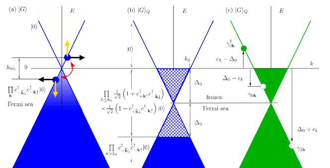
Figure 1: Fermi sea reconstruction in the vicinity of the crossing bands. a The normal ground state, $|G\rangle$. A BCS-like electron-electron pairing occurs between the states having antiparallel momenta (black arrows) and spins (yellow arrows). The energy window $\hbar\omega_{c}$ is determined by the pairing mechanism (phonon- or plasmon-assisted). The blue gradient illustrates electron population at finite temperature. b The correlated ground state, $|G\rangle_{Q}$, splits into two sectors with $k\leq k_{0}$ and $k>k_{0}$. The former has a BCS-like structure, whereas the latter represents normal electrons, and the two sectors together can be seen as a “BCS ice” floating on a Fermi liquid. The thickness of the “ice” layer is $2\Delta_{0}$ with $\Delta_{0}$ being the self-consistent order parameter. c The correlated ground state and excitations in terms of the quasiparticle operators, $\gamma_{0{\mathbf{k}}}$ and $\gamma_{1{\mathbf{k}}}$. The $\gamma_{1{\mathbf{k}}}$-excitations are gapped by $\Delta_{0}$ even though the overall spectrum is gapless.

The mathematical expression for the paired state is

$$|G\rangle_{Q}=\prod\limits_{k>k_{0}}\left(c_{-\bar{\mathbf{k}}\downarrow}^{\dagger}c_{-{\mathbf{k}}\uparrow}^{\dagger}\right)$$ (1)

$$\times\prod\limits_{k\leq k_{0}}\left[\frac{1}{\sqrt{2}}\left(1+c_{+{\mathbf{k}}\uparrow}^{\dagger}c_{-\bar{\mathbf{k}}\downarrow}^{\dagger}\right)\frac{1}{\sqrt{2}}\left(1-c_{+\bar{\mathbf{k}}\downarrow}^{\dagger}c_{-{\mathbf{k}}\uparrow}^{\dagger}\right)\right]|0\rangle,$$

where $|0\rangle$ denotes the electron vacuum, $c_{\kappa{\mathbf{k}}\sigma}^{\dagger}$ is the electronic creation operator for a given band index $\kappa=\{\pm\}$, spin $\sigma=\{\uparrow\downarrow\}$, and wave vector ${\mathbf{k}}$ ($|{\mathbf{k}}|\equiv k$) with $\bar{\mathbf{k}}\equiv-{\mathbf{k}}$. This state is a spin singlet. The wave vector $k_{0}=\Delta_{0}/(\hbar v)$ (with the order parameter $\Delta_{0}$, band velocity $v$, and Planck constant $\hbar$) separates the “paired” and normal electrons in $k$-space and plays the same role as the inverse coherence length in the BCS state Parks1969 . In contrast to a conventional BCS state, however, there is no quasiparticle gap – see Fig. 1c. Another important difference is that while the conventional BCS state occurs for arbitrarily weak attractive interaction, the present state requires a certain minimal interaction strength in order to make up for the energy of formation of the pseudo-Fermi surface. Furthermore, once the critical interaction is achieved, the order parameter $\Delta_{0}$ (i.e., the energy of the pseudo-Fermi surface) is larger than the characteristic range of band energies over which the attractive interaction is operative: $\Delta_{0}>\hbar\omega_{c}/2$, where $\omega_{c}$ is a cut-off frequency, see Fig. 1b.

A natural question at this point is whether the unconventional state (1) has a chance to win the energy competition against the conventional BCS state. Considering the situation on the band theory level without taking into account the structure of single-electron states we expect the BCS state to win PRL2008BCS . However, the single-electron state structure may impose additional restrictions on electron pairing. In the case of a honeycomb lattice, the single-electron states forming the conical band-crossings in the opposite corners of the first Brillouin zone are not equivalent but represent time-reversal reflections of each other. Hence, if a pairing involves time-reversal states, then we must take into account the difference between single-electron state structure in the opposite corners of the first Brillouin zone topological2022 . We will show that intervalley electron pairing provided by attractive on-site interactions on a honeycomb lattice is equivalent to the cross-band pairing introduced in Fig. 1a. Neither time-reversal invariance nor sublattice equivalence (parity-reversal invariance) is broken in our model. We do not make assumptions about the microscopic origin of the attractive on-site interaction: we simply assume that it exists.

One way to facilitate the formation of the new paired state is to create a high density of states by flattening the electron bands near the crossing point. This can be done by twisting adjacent graphene layers in double-layer cao_unconventional_2018 ; cao_correlated_2018 ; yankowitz_2019_tuning and multilayer shen2020correlated ; liu2020tunable ; cao2020tunable ; xu2021tunable ; he2021symmetry structures, which indeed have two equivalent valleys at the Fermi level. Here the interaction energy can greatly exceed the band energy of the electrons and drive the system into various strongly correlated phases, including magnetic, superconducting, and Mott insulator phases. Most remarkably from our point of view, twisted double bilayer graphene (TDBG) exhibits a non-superconducting resistivity drop supposedly indicating a phase transition to an unknown strongly correlated state he2021symmetry . At the same time, we expect the new paired state will have no unusual signatures in spectroscopy measurements, unlike a superconductor or a Mott insulator. We will show that this phenomenology could be a manifestation of the unconventional state (1).

In this work, we demonstrate how the cross-band pairing shown in Fig. 1a can occur for electrons on a honeycomb lattice and deduce a Hamiltonian with the many-body ground state (1). We find a self-consistent equation for the order parameter $\Delta_{0}$ shown in Fig. 1b. We demonstrate that the available quasiparticle excitation channels shown in Fig. 1c forbid electron scattering on disorder.

Results and Discussion

The model Hamiltonian

The cross-band pairing assumed in the introduction can be deduced from a lattice model. The conical electronic bands can be obtained from the low-energy expansion of the tight-binding Hamiltonian on a honeycomb lattice Mott-on-honeycomb2020 . As the honeycomb lattice comprises two sublattices the Hamiltonian represents a 2$\times$2 matrix in the sublattice basis. There are also two non-equivalent valleys, which are time-reversal reflections of each other. For the spin-up electrons we write the Hamiltonian as

$$H_{\uparrow} =\sum\limits_{\mathbf{k}}\left(c_{A\mathbf{k}\uparrow}^{\dagger}c_{B\mathbf{k}\uparrow}^{\dagger}\right)\left(\begin{array}[]{cc}0&\epsilon_{k}e^{-i\theta}\\ \epsilon_{k}e^{i\theta}&0\end{array}\right)\left(\begin{array}[]{c}c_{A\mathbf{k}\uparrow}\\ c_{B\mathbf{k}\uparrow}\end{array}\right)$$ (11)

$$+\sum\limits_{\mathbf{k}}\left(c_{A\mathbf{\bar{k}}\uparrow}^{\dagger}c_{B\mathbf{\bar{k}}\uparrow}^{\dagger}\right)\left(\begin{array}[]{cc}0&-\epsilon_{k}e^{i\theta}\\ -\epsilon_{k}e^{-i\theta}&0\end{array}\right)\left(\begin{array}[]{c}c_{A\mathbf{\bar{k}}\uparrow}\\ c_{B\mathbf{\bar{k}}\uparrow}\end{array}\right),$$

and for spin-down electrons it reads

$$H_{\downarrow} =\sum\limits_{\mathbf{k}}\left(c_{A\mathbf{k}\downarrow}^{\dagger}c_{B\mathbf{k}\downarrow}^{\dagger}\right)\left(\begin{array}[]{cc}0&\epsilon_{k}e^{-i\theta}\\ \epsilon_{k}e^{i\theta}&0\end{array}\right)\left(\begin{array}[]{c}c_{A\mathbf{k}\downarrow}\\ c_{B\mathbf{k}\downarrow}\end{array}\right)$$ (21)

$$+\sum\limits_{\mathbf{k}}\left(c_{A\mathbf{\bar{k}}\downarrow}^{\dagger}c_{B\mathbf{\bar{k}}\downarrow}^{\dagger}\right)\left(\begin{array}[]{cc}0&-\epsilon_{k}e^{i\theta}\\ -\epsilon_{k}e^{-i\theta}&0\end{array}\right)\left(\begin{array}[]{c}c_{A\mathbf{\bar{k}}\downarrow}\\ c_{B\mathbf{\bar{k}}\downarrow}\end{array}\right),$$

where $c_{A(B)\mathbf{k}\uparrow(\downarrow)}^{\dagger}$ creates a spin-up (spin-down) electron on a sublattice A(B). Here, $\epsilon_{k}=\hbar vk$, $k=\sqrt{k_{x}^{2}+k_{y}^{2}}$, $\hbar v=3|t|a_{0}/2$ with $t$ and $a_{0}$ being the inter-site distance and hopping, respectively, $\tan\theta=k_{y}/k_{x}$, and $k_{x,y}$ are the wave vector components. Note that the wave vector $\mathbf{\bar{k}}$ is counted from the opposite corner of the first Brillouin zone, but it is has the same absolute value as $\mathbf{k}$, hence, no valley index in $\epsilon_{k}$ and $\theta$ is needed.

We assume that electron-electron pairing occurs between the time-reversal states that implies intervalley pairing in the case of a honeycomb lattice. Hence, the pairing Hamiltonian can be written as

$$H_{\mathrm{pair}} = -V_{0}\sum\limits_{\mathbf{k},\mathbf{k}^{\prime}}\left(c^{\dagger}_{A\mathbf{k}\uparrow}c^{\dagger}_{A\mathbf{\bar{k}}\downarrow}c_{A\mathbf{\bar{k}}^{\prime}\downarrow}c_{A\mathbf{k}^{\prime}\uparrow}\right.$$ (22)

$$\left.+c^{\dagger}_{B\mathbf{k}\uparrow}c^{\dagger}_{B\mathbf{\bar{k}}\downarrow}c_{B\mathbf{\bar{k}}^{\prime}\downarrow}c_{B\mathbf{k}^{\prime}\uparrow}+c^{\dagger}_{A\mathbf{k}\downarrow}c^{\dagger}_{A\mathbf{\bar{k}}\uparrow}c_{A\mathbf{\bar{k}}^{\prime}\uparrow}c_{A\mathbf{k}^{\prime}\downarrow}\right.$$

$$\left.+c^{\dagger}_{B\mathbf{k}\downarrow}c^{\dagger}_{B\mathbf{\bar{k}}\uparrow}c_{B\mathbf{\bar{k}}^{\prime}\uparrow}c_{B\mathbf{k}^{\prime}\downarrow}\right).$$

Equation (22) resembles the BCS pairing Hamiltonian flensberg2004many with the electronic creation and annihilation operators redefined specifically on a honeycomb lattice. The meaning of $V_{0}$ is therefore not the same as in the BCS theory, it should be seen as an on-site pairing strength in the spirit of the Hubbard model. The summation limits over $\mathbf{k}$ and $\mathbf{k}^{\prime}$ are determined by the band width rather than the Debye frequency relevant for the phonon-assisted pairing in the BCS theory. As we are working within the Dirac cone approximation for electron states, the summation limits in Eq. (22) are given by a certain cut-off energy $\hbar\omega_{c}$ as $|\mathbf{k}|$, $|\mathbf{k}^{\prime}|$ $\leq\omega_{c}/2v$, see Fig. 1a. We discuss the reasonable values for $\hbar\omega_{c}$ in application to TDBG below. In the following equations involving summation over the wave vector the cut-off is always implicit.

The total Hamiltonian, $H$, is a sum of Eqs. (11), (21), and (22). Since no intravalley pairing is assumed, it is convenient to rewrite the model Hamiltonian as a sum of two non-interacting terms given by

$$H = H_{\uparrow}+H_{\downarrow}+H_{\mathrm{int}}$$ (23)

$$= H_{\uparrow\downarrow}+H_{\downarrow\uparrow},$$

where

$$H_{\uparrow\downarrow}=\sum\limits_{\mathbf{k}}\epsilon_{k}\left(e^{-i\theta}c_{A\mathbf{k}\uparrow}^{\dagger}c_{B\mathbf{k}\uparrow}+e^{i\theta}c_{B\mathbf{k}\uparrow}^{\dagger}c_{A\mathbf{k}\uparrow}\right.$$ (24)

$$\left.-e^{i\theta}c_{A\mathbf{\bar{k}}\downarrow}^{\dagger}c_{B\mathbf{\bar{k}}\downarrow}-e^{-i\theta}c_{B\mathbf{\bar{k}}\downarrow}^{\dagger}c_{A\mathbf{\bar{k}}\downarrow}\right)$$

$$-V_{0}\sum\limits_{\mathbf{k},\mathbf{k}^{\prime}}\left(c^{\dagger}_{A\mathbf{k}\uparrow}c^{\dagger}_{A\mathbf{\bar{k}}\downarrow}c_{A\mathbf{\bar{k}}^{\prime}\downarrow}c_{A\mathbf{k}^{\prime}\uparrow}+c^{\dagger}_{B\mathbf{k}\uparrow}c^{\dagger}_{B\mathbf{\bar{k}}\downarrow}c_{B\mathbf{\bar{k}}^{\prime}\downarrow}c_{B\mathbf{k}^{\prime}\uparrow}\right),$$

and $H_{\downarrow\uparrow}$ can be written by swapping the spin indices. The properties of $H_{\uparrow\downarrow}$ and $H_{\downarrow\uparrow}$ are identical. We focus on $H_{\uparrow\downarrow}$ in what follows.

To cast Eq. (24) into a matrix form we employ a BCS-like mean-field approximation with the order parameter given by

$$\Delta_{A,B} = V_{0}\sum_{\mathbf{k}}\langle c^{\dagger}_{A,B\mathbf{k}\uparrow}c^{\dagger}_{A,B\mathbf{\bar{k}}\downarrow}\rangle$$ (25)

$$= \Delta_{0},$$

where the sublattice equivalence has been assumed. Equation (24) can be then transformed as

$$H_{\uparrow\downarrow}^{MF} = \sum\limits_{\mathbf{k}}\left[\Delta_{0}\left(\langle c_{A\mathbf{\bar{k}}\downarrow}c_{A\mathbf{k}\uparrow}\rangle+\langle c_{B\mathbf{\bar{k}}\downarrow}c_{B\mathbf{k}\uparrow}\rangle\right)\right.$$ (31)

$$\left.+\left(c_{A\mathbf{k}\uparrow}^{\dagger}c_{B\mathbf{k}\uparrow}^{\dagger}c_{A\mathbf{\bar{k}}\downarrow}c_{B\mathbf{\bar{k}}\downarrow}\right)H_{k}^{MF}\left(\begin{array}[]{c}c_{A\mathbf{k}\uparrow}\\ c_{B\mathbf{k}\uparrow}\\ c_{A\mathbf{\bar{k}}\downarrow}^{\dagger}\\ c_{B\mathbf{\bar{k}}\downarrow}^{\dagger}\end{array}\right)\right],$$

where

$$H_{k}^{MF}=\left(\begin{array}[]{cccc}0&\epsilon_{k}e^{-i\theta}&-\Delta_{0}&0\\ \epsilon_{k}e^{i\theta}&0&0&-\Delta_{0}\\ -\Delta_{0}&0&0&\epsilon_{k}e^{-i\theta}\\ 0&-\Delta_{0}&\epsilon_{k}e^{i\theta}&0\end{array}\right).$$ (32)

The matrix $H_{k}^{MF}$ can be diagonalized straightforwardly but it is instructive to bring Eq. (31) into a block-diagonal form using the following transformation

$$c_{A\mathbf{k}\uparrow}^{\dagger} = \frac{1}{\sqrt{2}}\left(c_{+\mathbf{k}\uparrow}^{\dagger}+c_{-\mathbf{k}\uparrow}^{\dagger}\right),$$ (33)

$$c_{B\mathbf{k}\uparrow}^{\dagger} = \frac{e^{-i\theta}}{\sqrt{2}}\left(c_{+\mathbf{k}\uparrow}^{\dagger}-c_{-\mathbf{k}\uparrow}^{\dagger}\right),$$ (34)

$$c_{A\mathbf{\bar{k}}\downarrow}^{\dagger} = \frac{1}{\sqrt{2}}\left(c_{-\mathbf{\bar{k}}\downarrow}^{\dagger}+c_{+\mathbf{\bar{k}}\downarrow}^{\dagger}\right),$$ (35)

$$c_{B\mathbf{\bar{k}}\downarrow}^{\dagger} = \frac{e^{i\theta}}{\sqrt{2}}\left(c_{-\mathbf{\bar{k}}\downarrow}^{\dagger}-c_{+\mathbf{\bar{k}}\downarrow}^{\dagger}\right).$$ (36)

Here, $c_{\pm\mathbf{k}\uparrow}^{\dagger}$ creates a spin-up electron in the conduction (valence) band with the dispersion $+\epsilon_{k}$ ($-\epsilon_{k}$), whereas $c_{\pm\mathbf{\bar{k}}\downarrow}^{\dagger}$ does the same with a spin-down state. The result can be written as $H^{MF}_{\uparrow\downarrow}=H^{MF}_{+}+H^{MF}_{-}$, where

$$H^{MF}_{+} = \sum\limits_{\mathbf{k}}\left[\Delta_{0}\langle c_{-\mathbf{\bar{k}}\downarrow}c_{+\mathbf{k}\uparrow}\rangle-\epsilon_{k}\right.$$ (42)

$$\left.+\left(c_{+\mathbf{k}\uparrow}^{\dagger}c_{-\mathbf{\bar{k}}\downarrow}\right)\left(\begin{array}[]{cc}\epsilon_{k}&-\Delta_{0}\\ -\Delta_{0}&\epsilon_{k}\end{array}\right)\left(\begin{array}[]{c}c_{+\mathbf{k}\uparrow}\\ c_{-\mathbf{\bar{k}}\downarrow}^{\dagger}\end{array}\right)\right],$$

$$H^{MF}_{-} = \sum\limits_{\mathbf{k}}\left[-\Delta_{0}\langle c_{-\mathbf{k}\uparrow}c_{+\mathbf{\bar{k}}\downarrow}\rangle-\epsilon_{k}\right.$$ (48)

$$\left.+\left(c_{+\mathbf{\bar{k}}\downarrow}^{\dagger}c_{-\mathbf{k}\uparrow}\right)\left(\begin{array}[]{cc}\epsilon_{k}&\Delta_{0}\\ \Delta_{0}&\epsilon_{k}\end{array}\right)\left(\begin{array}[]{c}c_{+\mathbf{\bar{k}}\downarrow}\\ c_{-\mathbf{k}\uparrow}^{\dagger}\end{array}\right)\right].$$

We have made use of the following relation

$$\langle c_{A\mathbf{\bar{k}}\downarrow}c_{A\mathbf{k}\uparrow}\rangle+\langle c_{B\mathbf{\bar{k}}\downarrow}c_{B\mathbf{k}\uparrow}\rangle=\langle c_{-\mathbf{\bar{k}}\downarrow}c_{+\mathbf{k}\uparrow}\rangle+\langle c_{+\mathbf{\bar{k}}\downarrow}c_{-\mathbf{k}\uparrow}\rangle.$$

The matrices in Eqs. (42) and (48) differ by the sign in front of the order parameter only. Most importantly, the on-site pairing introduced by Eq. (22) and explicitly seen in the mean-field Eqs. (31), (32) has turned out to be equivalent to the cross-band pairing, as shown in Fig. 1a. The conventional intraband BCS-like pairing does not occur in such a formulation. We therefore do not use the conventional BCS state as a reference ground state, we are benchmarking with the normal ground state instead.

The order parameter equation

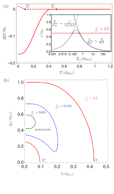
Figure 2: Correlated state energy. (a) The thermodynamic potential difference $\Delta\Omega$ between the correlated and normal states in units of $\Omega_{0}=\hbar\omega_{c}^{3}/(16\pi v^{2})$. There are two possible solutions of the order parameter equation but only the one with $\Delta\Omega<0$ makes physical sense for $T<T_{c}$. Inset: Graphical solution of Eq. (59). The red horizontal line intersects the blue curve twice indicating two critical temperatures. Both critical temperatures can be estimated from the simple relations given in the figure and depicted by the dashed lines. (b) Solutions of the order parameter equation, Eq. (58). The critical temperatures $T_{c}^{\prime}$ and $T_{c}$ exists if and only if either the bands are flat or interactions are strong enough, $v/v_{0}\lesssim 0.55$. (Here, $v_{0}$ is the interaction parameter, see the text.) At $0.55\lesssim v/v_{0}\lesssim 0.7$ the solutions are metastable, and no solution exists if $v/v_{0}\gtrsim 0.7$.

The order parameter equation can be derived from Eq. (25) using the Bogoljubov transformation diagonalizing Eq. (32), as shown in Methods. At this point, however, it is convenient to diagonalize $H^{MF}_{+}$ and $H^{MF}_{-}$ separately and write the order parameter as

$$\Delta_{0} = V_{0}\sum_{\mathbf{k}}\langle c_{-\mathbf{\bar{k}}\downarrow}c_{+\mathbf{k}\uparrow}\rangle$$ (49)

$$\equiv V_{0}\sum_{\mathbf{k}}\langle c_{+\mathbf{\bar{k}}\downarrow}c_{-\mathbf{k}\uparrow}\rangle.$$

The respective Bogoljubov transformation are given by

$$c_{+\mathbf{k}\uparrow}^{\dagger}=\frac{1}{\sqrt{2}}\left(\gamma_{0\mathbf{k}}^{\dagger}+\gamma_{1\mathbf{k}}\right),\quad c_{+\mathbf{k}\uparrow}=\frac{1}{\sqrt{2}}\left(\gamma_{0\mathbf{k}}+\gamma_{1\mathbf{k}}^{\dagger}\right),$$

$$c_{-\mathbf{\bar{k}}\downarrow}^{\dagger}=\frac{1}{\sqrt{2}}\left(\gamma_{0\mathbf{k}}-\gamma_{1\mathbf{k}}^{\dagger}\right),\quad c_{-\mathbf{\bar{k}}\downarrow}=\frac{1}{\sqrt{2}}\left(\gamma_{0\mathbf{k}}^{\dagger}-\gamma_{1\mathbf{k}}\right),$$

$$c_{+\bar{\mathbf{k}}\downarrow}^{\dagger}=\frac{1}{\sqrt{2}}\left(\beta_{1\mathbf{k}}+\beta_{0\mathbf{k}}^{\dagger}\right),\quad c_{+\bar{\mathbf{k}}\downarrow}=\frac{1}{\sqrt{2}}\left(\beta_{1\mathbf{k}}^{\dagger}+\beta_{0\mathbf{k}}\right),$$

$$c_{-\mathbf{k}\uparrow}^{\dagger}=\frac{1}{\sqrt{2}}\left(\beta_{1\mathbf{k}}^{\dagger}-\beta_{0\mathbf{k}}\right),\quad c_{-\mathbf{k}\uparrow}=\frac{1}{\sqrt{2}}\left(\beta_{1\mathbf{k}}-\beta_{0\mathbf{k}}^{\dagger}\right),$$

and the diagonalized $H^{MF}_{+}$ and $H^{MF}_{-}$ read

$$H^{MF}_{+} = \sum_{\mathbf{k}}\Delta_{0}\left[1+\frac{1}{2}\left(\langle\gamma_{0\mathbf{k}}^{\dagger}\gamma_{0\mathbf{k}}\rangle+\langle\gamma_{1\mathbf{k}}^{\dagger}\gamma_{1\mathbf{k}}\rangle-1\right)\right]$$

$$+ \sum_{\mathbf{k}}\left[\left(\epsilon_{k}-\Delta_{0}\right)\gamma_{0\mathbf{k}}^{\dagger}\gamma_{0\mathbf{k}}+\left(-\epsilon_{k}-\Delta_{0}\right)\gamma_{1\mathbf{k}}^{\dagger}\gamma_{1\mathbf{k}}\right],$$

$$H^{MF}_{-} = \sum_{\mathbf{k}}\Delta_{0}\left[1+\frac{1}{2}\left(\langle\beta_{0\mathbf{k}}^{\dagger}\beta_{0\mathbf{k}}\rangle+\langle\beta_{1\mathbf{k}}^{\dagger}\beta_{1\mathbf{k}}\rangle-1\right)\right]$$

$$+ \sum_{\mathbf{k}}\left[\left(\epsilon_{k}-\Delta_{0}\right)\beta_{0\mathbf{k}}^{\dagger}\beta_{0\mathbf{k}}+\left(-\epsilon_{k}-\Delta_{0}\right)\beta_{1\mathbf{k}}^{\dagger}\beta_{1\mathbf{k}}\right].$$

Hence, both Hamiltonians $H^{MF}_{+}$ and $H^{MF}_{-}$ have the same spectrum given by two branches $E_{0k}=\epsilon_{k}-\Delta_{0}$ and $E_{1k}=-\epsilon_{k}-\Delta_{0}$ for quasiparticles of type “0” and “1” respectively.

One can prove directly that $|G\rangle_{Q}$ given by Eq. (1) is the ground state of $H^{MF}_{\uparrow\downarrow}$. Acting with either of $\gamma_{0{\mathbf{k}}}^{\dagger}$ ($k>k_{0}$), $\gamma_{0{\mathbf{k}}}$ ($k\leq k_{0}$), $\gamma_{1{\mathbf{k}}}$ on $|G\rangle_{Q}$ creates an excited state with the positive excitation energies indicated in Fig. 1c. Quite remarkably, the quasiparticle spectrum has two branches with excitation energies $|\epsilon_{k}+\Delta|$ and $|\epsilon_{k}-\Delta|$. At variance with a conventional BCS state, the second excitation branch is gapless. Doing the same with either of $\gamma_{0{\mathbf{k}}}$ ($k>k_{0}$), $\gamma_{0{\mathbf{k}}}^{\dagger}$ ($k\leq k_{0}$), $\gamma_{1{\mathbf{k}}}^{\dagger}$ on $|G\rangle_{Q}$ annihilates the ground state. The same is true for $\beta_{0,1{\mathbf{k}}}^{\dagger}$ and $\beta_{0,1{\mathbf{k}}}$.

The order parameter equation explicitly reads

$$\Delta_{0} = \frac{V_{0}}{2}\sum_{\mathbf{k}}\left(\langle\gamma_{0{\mathbf{k}}}^{\dagger}\gamma_{0{\mathbf{k}}}\rangle+\langle\gamma_{1{\mathbf{k}}}^{\dagger}\gamma_{1{\mathbf{k}}}\rangle-1\right)$$ (54)

$$= \frac{V_{0}}{2}\sum_{\mathbf{k}}\left[n_{F}(E_{0k})-n_{F}(-E_{1k})\right],$$

where $n_{F}$ is the Fermi-Dirac distribution. The same order parameter equation can be derived in terms of $\beta_{0,1{\mathbf{k}}}^{\dagger}$, $\beta_{0,1{\mathbf{k}}}$. In the limit of $\Delta_{0}\to 0$, Eq. (54) takes the form suitable for determining the critical temperature $T_{c}$ as

$$\frac{4T_{c}}{V_{0}}=\sum_{\mathbf{k}}\frac{1}{\cosh^{2}\left(\hbar vk/2T_{c}\right)}.$$ (55)

The order parameter has been derived within the static approximation. The retardation effects could in principle be taken into account by solving the Eliashberg equations, which we did in our previous paper Girish2020 . However, the retardation effects are generally found to facilitate pairing, if pairing occurs at the static level. Hence, the qualitative outcomes of Eq. (54) will not be compromised. In fact, one could think that for practical purposes all the effects of retardation are already included in our effective attractive interaction $V_{0}$. The mass renormalization effects could also be taken into account in the spirit of our previous work tang2018role . However, there is no need to do that because it is known that on-site interaction for electrons on a honeycomb lattice does not influence asymptotic infrared properties of the model with respect to the unperturbed non-interacting case giuliani2010two .

Manifestation of the paired state

In the conventional superconducting BCS model, the operators $\gamma_{0,1{\mathbf{k}}}$ acting on the ground state change the average particle number by a factor $\propto u_{\mathbf{k}}^{2}-v_{\mathbf{k}}^{2}$, which can be seen as a signature of the BCS superconducting state Tinkham1975 . The factor obviously vanishes in our case ($u_{\mathbf{k}}=v_{\mathbf{k}}=1/\sqrt{2}$) indicating that the state $|G\rangle_{Q}$ is not a conventional BCS state. The Bogoliubov transformation (LABEL:bog1–LABEL:bog2) depends on neither $\epsilon_{k}$ nor $\Delta_{0}$. The spectrum remains gapless and the quasiparticle density of states is the same as in the non-interacting case, regardless the order parameter value. Hence, we are not able to distinguish between our normal and correlated states spectroscopically.

Nevertheless, electron pairing may influence electron scattering and, as a consequence, electrical conductivity. Let us consider the non-magnetic disorder Hamiltonian given by $H^{\mathrm{dis}}=H^{\mathrm{dis}}_{\uparrow\downarrow}+H^{\mathrm{dis}}_{\downarrow\uparrow}$, where

$$H^{\mathrm{dis}}_{\uparrow\downarrow}=\sum\limits_{{\mathbf{k}},{\mathbf{k}}^{\prime},\kappa,\kappa^{\prime}}U_{{\mathbf{k}}{\mathbf{k}}^{\prime}}\left(c_{\kappa^{\prime}{\mathbf{k}}^{\prime}\uparrow}^{\dagger}c_{\kappa{\mathbf{k}}\uparrow}+c_{\kappa^{\prime}\bar{{\mathbf{k}}}^{\prime}\downarrow}^{\dagger}c_{\kappa\bar{{\mathbf{k}}}\downarrow}\right)$$ (56)

and $H^{\mathrm{dis}}_{\downarrow\uparrow}$ can be written by swapping the spin indices. Here, $U_{{\mathbf{k}}{\mathbf{k}}^{\prime}}$ is the matrix element of a smooth potential unable to induce intervalley scattering. Eq. (56) can be rewritten in terms of the quasiparticle operators according to the Bogoliubov transformation (LABEL:bog1), (LABEL:bog2) as

$$H^{\mathrm{dis}}_{\uparrow\downarrow} = \sum\limits_{{\mathbf{k}},{\mathbf{k}}^{\prime},\kappa,\kappa^{\prime}}U_{{\mathbf{k}}{\mathbf{k}}^{\prime}}\left(c_{\kappa^{\prime}{\mathbf{k}}^{\prime}\uparrow}^{\dagger}c_{\kappa{\mathbf{k}}\uparrow}+c_{\kappa^{\prime}\bar{{\mathbf{k}}}^{\prime}\downarrow}^{\dagger}c_{\kappa\bar{{\mathbf{k}}}\downarrow}\right)$$ (57)

$$= \sum\limits_{{\mathbf{k}},{\mathbf{k}}^{\prime}}U_{{\mathbf{k}}{\mathbf{k}}^{\prime}}\left(\gamma_{0\mathbf{k}^{\prime}}^{\dagger}\gamma_{1\mathbf{k}}^{\dagger}+\gamma_{1\mathbf{k}^{\prime}}\gamma_{0\mathbf{k}}+\beta_{0\mathbf{k}^{\prime}}^{\dagger}\beta_{1\mathbf{k}}^{\dagger}+\beta_{1\mathbf{k}^{\prime}}\beta_{0\mathbf{k}}\right.$$

$$\left.+\gamma_{1\mathbf{k}^{\prime}}\beta_{1\mathbf{k}}-\gamma_{0\mathbf{k}^{\prime}}^{\dagger}\beta_{0\mathbf{k}}^{\dagger}+\beta_{1\mathbf{k}^{\prime}}^{\dagger}\gamma_{1\mathbf{k}}^{\dagger}-\beta_{0\mathbf{k}^{\prime}}\gamma_{0\mathbf{k}}\right).$$

The same transformation can be done with $H^{\mathrm{dis}}_{\downarrow\uparrow}$. Equation (57) suggests that conventional scattering processes (i.e. annihilation of one quasiparticle in a state with wave vector $\mathbf{k}$ and subsequent creation of another quasiparticle in a state with wave vector $\mathbf{k}^{\prime}$) is not possible. The only possible processes must be accompanied by creation (or annihilation) of two quasiparticles at once with wave vectors $\mathbf{k}$ and $\mathbf{k}^{\prime}$. Such processes require energy change and cannot be seen as elastic scattering. In fact, the quasiparticle states are protected from elastic scattering by the symmetry of the Bogoliubov transformation having equal coherences. The symmetry can be broken by shifting the Fermi level away from the band-crossing but the effect is negligible as long as the shift is much less than $\hbar\omega_{c}$, see Methods.

Transition to the paired state

Our theory does not involve the dimensionality of the wave vector ${\mathbf{k}}$ explicitly and can be used in any number of dimensions. However, solving Eqs. (54) and (55) explicitly involves a density of states (DOS) which, in turn, depends on dimensionality of the problem. In a two-dimensional case, Eq. (54) takes the following form

$$\frac{2\Delta_{0}}{\hbar\omega_{c}}= \frac{V_{0}\omega_{c}}{8\pi\hbar v^{2}}\int\limits_{0}^{1}dxx\left[n_{F}\left(x\frac{\hbar\omega_{c}}{2}-\Delta_{0}\right)\right.$$ (58)

$$\left.-n_{F}\left(x\frac{\hbar\omega_{c}}{2}+\Delta_{0}\right)\right].$$

At $T=0$, we have $\Delta_{0}=V_{0}\omega_{c}^{2}/(32\pi v^{2})$, if $\Delta_{0}>\hbar\omega_{c}/2$, and $\Delta_{0}=8\pi\hbar^{2}v^{2}/V_{0}$, if $\Delta_{0}\leq\hbar\omega_{c}/2$. Most importantly, there is no solution at all as long as $V_{0}<16\pi\hbar v^{2}/\omega_{c}$. This is again in contrast with the conventional BCS gap equation that has a solution for any pairing potential strength.

The critical temperature can be found either from Eq. (55) or Eq. (58) by setting $\Delta_{0}\to 0$ and integrating over $x$. Since it is the velocity $v$ that is controllable in twisted multilayer graphene, it is convenient to introduce the interaction parameter as $v_{0}=\sqrt{\omega_{c}V_{0}/(8\pi\hbar)}$, and the result reads

$$\frac{v^{2}}{v_{0}^{2}}=\tanh\left(\frac{\hbar\omega_{c}}{4T_{c}}\right)-\frac{4T_{c}}{\hbar\omega_{c}}\ln\cosh\left(\frac{\hbar\omega_{c}}{4T_{c}}\right),$$ (59)

The higher critical temperature can be estimated as ${T_{c}}/{\hbar\omega_{c}}\sim{v_{0}^{2}}/{8v^{2}}$, whereas the lower one reads ${T^{\prime}_{c}}/{\hbar\omega_{c}}\sim{v^{2}}/(4v_{0}^{2}\ln 2)$. Solutions of Eqs. (58) and (59) are shown in Fig. 2.

To understand the meaning of $T_{c}$ and $T^{\prime}_{c}$, we compare the thermodynamic potential of our correlated state, $\Omega_{Q}$, with that of a normal state, $\Omega_{N}$. We start from the partition function for a given spin channel $Z=\mathrm{Tr}\left[e^{-{H^{MF}_{\uparrow\downarrow}}/{T}}\right]$, which in our case explicitly reads

$$Z=\prod\limits_{k}\left[\left(1+e^{-\frac{\epsilon_{k}-\Delta_{0}}{T}}\right)\left(1+e^{-\frac{-\epsilon_{k}-\Delta_{0}}{T}}\right)\right]$$

$$\times e^{-\frac{\Delta_{0}}{2T}\sum_{k}\left[n_{F}(\epsilon_{k}-\Delta_{0})-n_{F}(\epsilon_{k}+\Delta_{0})+2\right]}.$$ (60)

We calculate $\Omega_{Q}=-T\ln Z$, and $\Omega_{N}$ is given by the same formula with $\Delta_{0}=0$. The difference $\Delta\Omega=\Omega_{Q}-\Omega_{N}$ is shown in Fig. 2(a). If $\Delta\Omega<0$, then the correlated state has lower energy than the normal one, and the electrons condense into that special state. Hence, the higher critical temperature $T_{c}$ indeed describes transition into a correlated phase having lower energy than the normal state. This is unlike the $T^{\prime}_{c}$ where no actual transition occurs. In fact, $T^{\prime}_{c}$ is due to the vanishing DOS at $\epsilon_{k}=0$. This pathological feature disappears for any other than linear band dispersion.

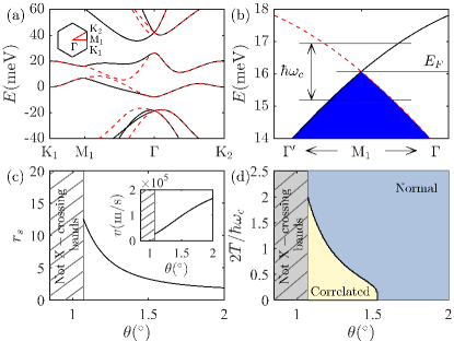
Figure 3: Correlated state of crossing bands in TDBG. a Calculated band structure of TDBG with the twist angle $\theta=1.33^{\circ}$ and without interlayer potential difference. The black (solid) and red (dashed) bands have different orbital characters. Inset shows the first Brilloin zone. b The X-shaped band-crossing along the $M_{1}$–$\Gamma$ direction with the Fermi level corresponding to the filling factor $\nu=1.75$. This particular crossing point dominates as having the highest DOS. $\Gamma^{\prime}$ represents the center of the neighboring first Brillouin zone. c Interaction parameter $r_{s}$ with $\bar{\epsilon}=6.85$ relevant for h-BN laturia2018dielectric ; geick1966normal . Inset shows electron velocity extracted from panel (b). d The phase diagram indicating the regions of correlated and normal electronic states. The critical temperature at $\theta=1.33^{\circ}$ is about $\hbar\omega_{c}/2$. Assuming $\hbar\omega_{c}=1.75$ meV we arrive at $T_{c}=10$K, which is in good agreement with the temperature reported in Ref. he2021symmetry at which the drop in resistivity occurs.

Our estimates of the pairing potential suggest that the electron-phonon coupling would be too weak to form a paired state of this new kind. Indeed, the typical value for the product between electronic DOS and $V_{0}$ lies between 0.2 and 0.4 in conventional superconductors Parks1969 , whereas in our case the critical interaction constant is one order of magnitude higher. It is however possible to satisfy the critical condition using a plasmon-assisted pairing with $V_{0}\sim e^{2}/\bar{\epsilon}$ with $\bar{\epsilon}$ being the effective dielectric constant. The coupling constant $r_{s}=e^{2}/(\bar{\epsilon}\hbar v)$ should then be seen as a rough characteristic of the Coulomb interaction strength responsible for the plasmon-assisted pairing. As $v$ is strongly reduced in twisted graphene multilayers shen2020correlated ; liu2020tunable ; cao2020tunable ; he2021symmetry ; xu2021tunable the coupling constant is elevated accordingly. The true plasmon-mediated pairing is described by the frequency-dependent Eliashberg gap equations, as shown in our previous paper Girish2020 .

Application to twisted double bilayer graphene

The electron transport measurements he2021symmetry clearly demonstrate a resistivity drop of twisted double bilayer graphene (TDBG) with twist angle $\theta=1.3^{\circ}$ and filling factor $\nu=1.7$ as temperature is lowered below 10 K. Figure 3(a,b) shows the relevant band structure with a conical intersection along the $M_{1}$–$\Gamma$ direction. The band-crossing intersects the Fermi level at $\theta=1.33^{\circ}$ and $\nu=1.75$ PhysRevB.99.235406 ; Lee2019Theory ; chu2021phonons ; PhysRevB.101.155149 ; PhysRevB.89.035405 ; doi:10.1073/pnas.1108174108 ; PhysRevX.8.031087 . The filling factor $\nu=4$ corresponds to a fully occupied band. There is no on-site energy difference between the layers. We refer to Methods for related technicalities.

To make connection between our predictions and TDBG we employ a toy (one-dimensional) version of our model. This allows us to get rid of the pathological metastable state at $T<T^{\prime}_{c}$ and parameterize the outcomes in terms of the physically transparent parameter $r_{s}=V_{0}/(\hbar v)$ with $V_{0}\sim e^{2}/\bar{\epsilon}$. Hence, Eq. (54) takes the form

$$\frac{2\Delta_{0}}{\hbar\omega_{c}} = \frac{r_{s}}{\pi}\int\limits_{0}^{1}dx\left[n_{F}\left(x\frac{\hbar\omega_{c}}{2}-\Delta_{0}\right)\right.$$ (61)

$$\left.-n_{F}\left(x\frac{\hbar\omega_{c}}{2}+\Delta_{0}\right)\right].$$

The critical temperature, $T_{c}$, can be estimated from Eq. (55) written as $r_{s}=\pi/\tanh[\hbar\omega_{c}/(4T_{c})]$. Obviously, $\tanh$ cannot be larger than 1, hence, $T_{c}$ does not exist as long as $r_{s}<\pi$. The order parameter at $T=0$ is given by $\Delta_{0}=\hbar\omega_{c}r_{s}/(2\pi)$ and is always larger than $\hbar\omega_{c}/2$. Figure 3(c) shows $r_{s}$ as a function of twist angle with $r_{s}>\pi$ at $\theta<1.5^{\circ}$ that suggests possible transition into our correlated state. Figure 3(d) shows the phase diagram with normal and correlated states. If $r_{s}>\pi$ and the temperature drops below $T_{c}$, then the upper layer of the Fermi sea turns into “ice”, and all the elastic scattering processes get turned off including charged impurities and other smooth defects. One is only left with magnetic impurities, if any, and inelastic scatterers, like phonons, which are much weaker at low temperatures. This is what might take place in TDBG at $T<T_{c}$ and manifest itself in the resistivity measurements he2021symmetry .

Outlook

The theory proposed above offers an interesting opportunity to decrease the ohmic resistivity of a semimetal without need to eliminate intrinsic impurities. The two crucial ingredients in this theory are (i) crossing electronic bands (conical intersection) and (ii) strong electron-electron pairing across the intersection provided by the lattice symmetry. The flatter the crossing bands are, the lower the critical interaction strength is. It is instructive to reformulate this criterion within a two-dimensional honeycomb lattice model with the nearest-neighbor hopping $t$ and on-site Hubbard interaction $U$ widely used to simulate behaviour of strongly correlated electrons. The energy cut-off is then given by the bandwidth, $\hbar\omega_{c}/2=3t$, and $V_{0}=UA$, where $A=3\sqrt{3}a_{0}^{2}/2$ is the unit cell area with $a_{0}$ being the lattice intersite distance Girish2020 . The low-energy expansion near one of the corners of the first Brillouin zone gives us the relation between $t$ and $v$ as $\hbar v=3ta_{0}/2$. Eq. (58) does not take into account valley degeneracy, hence, the integral in Eq. (58) must be doubled, and the equation has a solution if and only if $V_{0}>8\pi\hbar v^{2}/\omega_{c}$, which can be rewritten in the lattice terms as $U/t>2\pi/\sqrt{3}$. The phase transition is therefore expected at $U/t\sim 3.6$ that is surprisingly close to the Mott transition at $U/t\sim 3.7$ found on the same lattice Mott-on-honeycomb2010 ; Mott-on-honeycomb2020 . Note, however, that the actual lattice realization of our model might require a modification of the simple on-site Hubbard pairing to be revealed beyond the simple mean-field theory proposed here.

Methods

Bogoliubov transformations

Bogoliubov transformations represent the main method of this work. We fist adduce the Bogoliubov transformation diagonalizing Hamiltonian (31). The matrix $H_{k}^{MF}$ can be diagonalized straightforwardly by means of the matrix $P$ given by

$$P=\frac{1}{2}\left(\begin{array}[]{cccc}-e^{-i\theta}&e^{-i\theta}&e^{-i\theta}&-e^{-i\theta}\\ 1&1&-1&-1\\ -e^{-i\theta}&e^{-i\theta}&-e^{-i\theta}&e^{-i\theta}\\ 1&1&1&1\end{array}\right).$$ (62)

The Bogoliubov transformation then reads

$$\left(\begin{array}[]{c}c_{A\mathbf{k}\uparrow}\\ c_{B\mathbf{k}\uparrow}\\ c_{A\mathbf{\bar{k}}\downarrow}^{\dagger}\\ c_{B\mathbf{\bar{k}}\downarrow}^{\dagger}\end{array}\right)=P\left(\begin{array}[]{c}\xi_{\mathbf{k}1}\\ \xi_{\mathbf{k}2}\\ \xi_{\mathbf{k}3}^{\dagger}\\ \xi_{\mathbf{k}4}^{\dagger}\end{array}\right),$$ (63)

and $H_{\uparrow\downarrow}^{MF}$ can be written in a canonical form as

$$H_{\uparrow\downarrow}^{MF} = \sum_{\mathbf{k}}\left[\Delta_{0}\left(2+\langle c_{A\mathbf{\bar{k}}\downarrow}c_{A\mathbf{k}\uparrow}\rangle+\langle c_{B\mathbf{\bar{k}}\downarrow}c_{B\mathbf{k}\uparrow}\rangle\right)\right.$$ (64)

$$- \left.(\epsilon_{k}+\Delta_{0})\xi_{\mathbf{k}1}^{\dagger}\xi_{\mathbf{k}1}+(\epsilon_{k}-\Delta_{0})\xi_{\mathbf{k}2}^{\dagger}\xi_{\mathbf{k}2}\right.$$

$$+ \left.(\epsilon_{k}-\Delta_{0})\xi_{\mathbf{k}3}^{\dagger}\xi_{\mathbf{k}3}-(\epsilon_{k}+\Delta_{0})\xi_{\mathbf{k}4}^{\dagger}\xi_{\mathbf{k}4}\right].$$

The order parameter equation (25) then reads

$$\Delta_{0} = \frac{V_{0}}{4}\sum_{\mathbf{k}}\left(\langle\xi_{\mathbf{k}1}^{\dagger}\xi_{\mathbf{k}1}\rangle+\langle\xi_{\mathbf{k}2}^{\dagger}\xi_{\mathbf{k}2}\rangle\right.$$ (65)

$$- \left.\langle\xi_{\mathbf{k}3}\xi_{\mathbf{k}3}^{\dagger}\rangle-\langle\xi_{\mathbf{k}4}\xi_{\mathbf{k}4}^{\dagger}\rangle\right)$$

$$= \frac{V_{0}}{2}\sum_{\mathbf{k}}\left[n_{F}(-\epsilon_{k}-\Delta_{0})+n_{F}(\epsilon_{k}-\Delta_{0})-1\right]$$

$$= \frac{V_{0}}{2}\sum_{\mathbf{k}}\left[n_{F}(\epsilon_{k}-\Delta_{0})-n_{F}(\epsilon_{k}+\Delta_{0})\right].$$

Note that Eq. (65) coincides with Eq. (54).

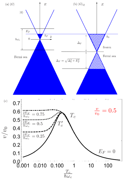
Figure 4: Fermi sea reconstruction at $E_{F}\neq 0$. a The normal ground state near the band crossing point at $E_{F}\neq 0$ and $T=0$. b The correlated ground state, $|G\rangle_{Q}$, splits into two sectors with $k\leq k_{0}$ and $k>k_{0}$. In contrast to the limit $E_{F}\to 0$ in Fig. 1, $k_{0}$ is given by $k_{0}=\Delta_{F}/(\hbar v)$, where $\Delta_{F}=\sqrt{\Delta_{0}^{2}+E_{F}^{2}}$. The Bogoliubov transformation (79) is not symmetric in this case. c The anomalous metastable state occurs at lower $T_{c}^{\prime}$ (cf. inset in Fig. 2a) with increasing $E_{F}$ and ceases to exist at $\sqrt{E_{F}/(\hbar\omega_{c})}>v/v_{0}$. In contrast, $T_{c}$ is much less sensitive to the variation of $E_{F}$.

Second, we notice that the symmetry of transformations (LABEL:bog1) and (LABEL:bog2) is broken once the Fermi energy does not intercept the band-crossing point ($E_{F}\neq 0$). To give an example, the mean-field Hamiltonian $H^{MF}_{+}$ then reads

$$H^{MF}_{+} = \sum_{\mathbf{k}}(c_{+\mathbf{k}\uparrow}^{\dagger}c_{-\mathbf{\bar{k}}\downarrow})\left(\begin{array}[]{cc}\epsilon_{k}-E_{F}&-\Delta_{0}\\ -\Delta_{0}&\epsilon_{k}+E_{F}\end{array}\right)\left(\begin{array}[]{c}c_{+\mathbf{k}\uparrow}\\ c_{-\mathbf{\bar{k}}\downarrow}^{\dagger}\end{array}\right)$$ (70)

$$+ \sum_{\mathbf{k}}\left(\Delta_{0}\langle c_{-\mathbf{\bar{k}}\downarrow}c_{+\mathbf{k}\uparrow}\rangle-\epsilon_{k}-E_{F}\right),$$ (71)

and its diagonalized version can be written as

$$H^{MF}_{+} = \sum_{\mathbf{k}}\left(\Delta_{0}\langle c_{-\mathbf{\bar{k}}\downarrow}c_{+\mathbf{k}\uparrow}\rangle+\Delta_{F}-E_{F}\right)$$

$$+ \sum_{\mathbf{k}}\left[\left(\epsilon_{k}-\Delta_{F}\right)\zeta_{0\mathbf{k}}^{\dagger}\zeta_{0\mathbf{k}}+\left(-\epsilon_{k}-\Delta_{F}\right)\zeta_{1\mathbf{k}}^{\dagger}\zeta_{1\mathbf{k}}\right].$$

Here, $\Delta_{F}=\sqrt{\Delta_{0}^{2}+E_{F}^{2}}$, and $\zeta_{0,1\mathbf{k}}^{\dagger}$ and $\zeta_{0,1\mathbf{k}}$ are the new quasiparticle creation and annihilation operators given by

$$\left(\begin{array}[]{c}c_{+\mathbf{k}\uparrow}\\ c_{-\mathbf{\bar{k}}\downarrow}^{\dagger}\end{array}\right)=\left(\begin{array}[]{cc}\cos\frac{\vartheta}{2}&\sin\frac{\vartheta}{2}\\ \sin\frac{\vartheta}{2}&-\cos\frac{\vartheta}{2}\end{array}\right)\left(\begin{array}[]{c}\zeta_{0\mathbf{k}}\\ \zeta_{1\mathbf{k}}^{\dagger}\end{array}\right),$$ (79)

where $\tan\vartheta=\Delta_{0}/E_{F}$. The structure of the correlated state is shown in Fig. 4a,b. Note, that the Bogoliubov transformation is not anymore symmetric (the quasiparticle weights are not equal) so that the scattering terms do not vanish in Eq. (56) completely. However, $E_{F}<\hbar\omega_{c}/2$ by definition, and $\Delta_{0}>\hbar\omega_{c}/2$ increases further with interactions. Hence, $\Delta_{0}\gg E_{F}$ and $\vartheta\sim\pi/2$, if interactions are strong enough. As a consequence, the transformation symmetry arguments hold in this limit.

The asymmetric Bogoliubov transformation also enters the gap equation that can be written in terms of $\Delta_{F}$ as

$$\Delta_{0} = \frac{V_{0}}{2}\sin\vartheta\sum_{\mathbf{k}}\left[n_{F}(\epsilon_{k}-\Delta_{F})-n_{F}(\epsilon_{k}+\Delta_{F})\right],$$

or

$$\Delta_{F} = \frac{V_{0}}{2}\sum_{\mathbf{k}}\left[n_{F}(\epsilon_{k}-\Delta_{F})-n_{F}(\epsilon_{k}+\Delta_{F})\right].$$

Increasing $E_{F}$ extends the Fermi surface and makes the Fermi sea behave in a normal way. Fig. 4c shows that the anomalous metastable state disappears once $E_{F}$ becomes higher than $\hbar\omega_{c}v^{2}/v_{0}^{2}$, compare with inset in Fig. 2a. In contrast, the true transition temperature $T_{c}$ is not sensitive to $E_{F}$.

Continuum model of TDBG

We adopt the continuum model described by Refs. PhysRevB.99.235406 ; Lee2019Theory ; chu2021phonons ; PhysRevB.101.155149 to compute the band structure employed in Fig. 3. TDBG is composed of two layers of AB stacking bilayer graphene with a small twisted angle $\theta$. In our calculation, the top (bottom) layer is rotated clockwise (anticlockwise) by $\theta/2$. We define the lattice vector $\mathbf{a}_{1}=a(1,0)$ and $\mathbf{a}_{2}=a(1/2,\sqrt{3}/2)$ before rotation, $a=0.246\mathrm{nm}$ is the lattice constant for graphene. The corresponding reciprocal lattice vectors are $\mathbf{a}_{1}^{*}=(2\pi/a)(1,-1/\sqrt{3})$ and $\mathbf{a}_{2}^{*}=(2\pi/a)(0,2/\sqrt{3})$. After the rotation, lattice vectors and reciprocal lattice vectors for $l$-th ($l$=1,2) layer become $\mathbf{a}_{i}^{(l)}=R(\mp\theta/2)\mathbf{a}_{i}$ and $\mathbf{a}_{i}^{*(l)}=R(\mp\theta/2)\mathbf{a}_{i}^{*}$, where $R(\pm\theta/2)$ is the rotation matrix. Within the approximation of small twisted angle, the approximately commensurate conditional is satisfied and the reciprocal lattice vectors are given by $\mathbf{G}_{i}^{\mathrm{M}}=\mathbf{a}_{i}^{*(1)}-\mathbf{a}_{i}^{*(2)}(i=1,2)$. In specific, $\mathbf{G}_{1}^{\mathrm{M}}=\frac{8\pi\sin{(\theta/2)}}{\sqrt{3}a}(-\frac{1}{2},-\frac{\sqrt{3}}{2})$ and $\mathbf{G}_{2}^{\mathrm{M}}=\frac{8\pi\sin{(\theta/2)}}{\sqrt{3}a}(1,0)$. Each layer of carbon atoms is labeled by $\mathbf{X}=A_{1},B_{1},\dots,A_{4},B_{4}$, where A, B represent sub-lattice indices and 1–4 are layer labels. The Bloch basis of $p_{z}$ orbitals is defined as $|\mathbf{k},\mathbf{X}\rangle=\sum_{\mathbf{R_{x}}}e^{i\mathbf{k}\cdot\mathbf{R_{x}}}$, where $\mathbf{k}$ is the two-dimensional Bloch wave vector, $|\mathbf{R}_{\mathbf{X}}\rangle$ is the atomic $p_{z}$ orbital at site $\mathbf{R}_{\mathbf{X}}$. The Hamiltonian of AB-AB stacking TDBG in continuum model can be expressed as PhysRevB.99.235406

$$H=\left(\begin{array}[]{cccc}H_{0}\left(\mathbf{k}_{1}\right)&g^{\dagger}\left(\mathbf{k}_{1}\right)&0&0\\ g\left(\mathbf{k}_{1}\right)&H_{0}^{\prime}\left(\mathbf{k}_{1}\right)&T^{\dagger}&0\\ 0&T&H_{0}\left(\mathbf{k}_{2}\right)&g^{\dagger}\left(\mathbf{k}_{2}\right)\\ 0&0&g\left(\mathbf{k}_{2}\right)&H_{0}^{\prime}\left(\mathbf{k}_{2}\right)\end{array}\right)+V,$$ (82)

in the basis of $\mathbf{X}=A_{1},B_{1},A_{2},B_{2},A_{1},B_{3},A_{4},B_{4}$, where $\boldsymbol{k}_{l}=R(\pm\theta/2)\left(\boldsymbol{k}-\boldsymbol{K}_{\xi}^{(l)}\right)$, $\mathbf{K}_{\pm}=\pm(4\pi/3\sqrt{3}a,0)$ and

$$H_{0}(\boldsymbol{k})=\left(\begin{array}[]{cc}0&-\hbar v_{0}k_{-}\\ -\hbar v_{0}k_{+}&\Delta\end{array}\right),$$ (83)

$$H_{0}^{\prime}(\boldsymbol{k})=\left(\begin{array}[]{cc}\Delta&-\hbar v_{0}k_{-}\\ -\hbar v_{0}k_{+}&0\end{array}\right),$$ (84)

$$g(\boldsymbol{k})=\left(\begin{array}[]{cc}\hbar v_{4}k_{+}&\gamma_{1}\\ \hbar v_{3}k_{-}&\hbar v_{4}k_{+}\end{array}\right),$$ (85)

where $k_{\pm}=\xi k_{x}\pm ik_{y}$, $\xi=\pm 1$ is the valley index. We take the phenomenological parameter extracted from Ref. PhysRevB.89.035405

$$\left(\gamma_{0},\gamma_{1},\gamma_{3},\gamma_{4},\Delta\right)=(2610,361,283,138,15)\mathrm{meV}$$ (86)

with the relationship $\hbar v_{i}=(\sqrt{3}/2)\gamma_{i}a$.

Figure 5: The influence of the interlayer potential difference $D$ on the band structure of TDBG at $\theta=1.33^{\circ}$. The solid and dashed line represent different valleys having opposite orbital characters.

The matrix $T$ represents the coupling between top layer and bottom layer doi:10.1073/pnas.1108174108 ; PhysRevX.8.031087

$$T = \left(\begin{array}[]{cc}u&u^{\prime}\\ u^{\prime}&u\end{array}\right)+\left(\begin{array}[]{cc}u&u^{\prime}\omega^{-\xi}\\ u^{\prime}\omega^{\xi}&u\end{array}\right)e^{i\xi\mathbf{G}_{1}^{\mathrm{M}}\cdot\mathbf{r}}$$ (94)

$$+\left(\begin{array}[]{cc}u&u^{\prime}\omega^{\xi}\\ u^{\prime}\omega^{-\xi}&u\end{array}\right)\times e^{i\xi\left(\mathbf{G}_{1}^{\mathrm{M}}+\mathbf{G}_{2}^{\mathrm{M}}\right)\cdot\mathbf{r}},$$

where $\omega=e^{2\pi/3}$, and we set $u=79.7\mathrm{meV}$, $u^{\prime}=97.9\mathrm{meV}$ due to relaxation effect PhysRevX.8.031087 .

Lastly, $V$ represents the on-site energy of each layer

$$V=\left(\begin{array}[]{cccc}\frac{3}{2}D\hat{1}&0&0&0\\ 0&\frac{1}{2}D\hat{1}&0&0\\ 0&0&-\frac{1}{2}D\hat{1}&0\\ 0&0&0&-\frac{3}{2}D\hat{1}\end{array}\right),$$ (95)

where $\hat{1}$ is the $2\times 2$ unit matrix, and $D$ represents the electrostatic interlayer energy difference.

The band structures of TDBG are computed in $k$-spaces. For a given Bloch vector $\boldsymbol{k}$ in the moiré Brillouin zone, there are many states associated with each other by interlayer coupling matrix $T$, which can be mapped by $\boldsymbol{k}+\mathrm{n}\boldsymbol{G}_{1}^{M}+\mathrm{m}\boldsymbol{G}_{2}^{M}$, where $n,m$ is an integer in a range of $[-N,N]$. In our calculation, we truncate the $N=4$, and the calculation is done independently for each valley. Fig. 5 shows the band structures of TDBG calculated by the continuum model for different values of $D$.

Data availability

The data mentioned in Methods is available from the corresponding author upon reasonable request.

Author contributions

M.T. proposed the mean-field model for crossing bands, performed all calculations, and wrote the first draft. L.P. applied the model to TDBG. M.T., G.S., G.V., and S.A. conceived the project and discussed the motivation and results. S.A. supervised the overall project.

Competing interests

All authors declare no competing interests.

Additional information

Correspondence and requests for materials should be addressed to Maxim Trushin.

References

• (1) 3. The theory of a Fermi liquid. Sov. Phys. JETP 3, 920 (1957).
• (2) Pomeranchuk, I. I. On the stability of a Fermi liquid. Sov. Phys. JETP 8, 361 (1959).
• (3) Stoner, E. C. Collective electron ferromagnetism. Proceedings of the Royal Society of London. Series A. Mathematical and Physical Sciences 165, 372–414 (1938).
• (4) Bardeen, J., Cooper, L. N. & Schrieffer, J. R. Theory of superconductivity. Phys. Rev. 108, 1175–1204 (1957).
• (5) Goerbig, M. & Montambaux, G. Dirac Fermions in Condensed Matter and Beyond, 25–53 (Springer International Publishing, Cham, 2017).
• (6) Burkov, A. A. & Balents, L. Weyl semimetal in a topological insulator multilayer. Phys. Rev. Lett. 107, 127205 (2011).
• (7) Novoselov, K. S. et al. Two-dimensional gas of massless dirac fermions in graphene. Nature 438, 197–200 (2005).
• (8) Xu, S.-Y. et al. Discovery of a weyl fermion semimetal and topological fermi arcs. Science 349, 613–617 (2015).
• (9) Lv, B. Q. et al. Experimental discovery of Weyl semimetal TaAs. Phys. Rev. X 5, 031013 (2015).
• (10) Kotov, V. N., Uchoa, B., Pereira, V. M., Guinea, F. & Castro Neto, A. H. Electron-electron interactions in graphene: Current status and perspectives. Rev. Mod. Phys. 84, 1067–1125 (2012).
• (11) Stauber, T. et al. Interacting electrons in graphene: Fermi velocity renormalization and optical response. Phys. Rev. Lett. 118, 266801 (2017).
• (12) Tang, H.-K. et al. The role of electron-electron interactions in two-dimensional Dirac fermions. Science 361, 570–574 (2018).
• (13) Roy, B. & Herbut, I. F. Unconventional superconductivity on honeycomb lattice: Theory of kekule order parameter. Phys. Rev. B 82, 035429 (2010).
• (14) Honerkamp, C. Density waves and Cooper pairing on the honeycomb lattice. Phys. Rev. Lett. 100, 146404 (2008).
• (15) Uchoa, B. & Castro Neto, A. H. Superconducting states of pure and doped graphene. Phys. Rev. Lett. 98, 146801 (2007).
• (16) Herbut, I. F. Interactions and phase transitions on graphene’s honeycomb lattice. Phys. Rev. Lett. 97, 146401 (2006).
• (17) Trushin, M. Collinear scattering of photoexcited carriers in graphene. Phys. Rev. B 94, 205306 (2016).
• (18) Lucas, A. & Fong, K. C. Hydrodynamics of electrons in graphene. Journal of Physics: Condensed Matter 30, 053001 (2018).
• (19) Parks, R. D. (ed.) Superconductivity (Marcel Dekker Inc., NY, 1969).
• (20) Kopnin, N. B. & Sonin, E. B. BCS superconductivity of Dirac electrons in graphene layers. Phys. Rev. Lett. 100, 246808 (2008).
• (21) Lo, C. F. B., Po, H. C. & Nevidomskyy, A. H. Inherited topological superconductivity in two-dimensional dirac semimetals. Phys. Rev. B 105, 104501 (2022).
• (22) Cao, Y. et al. Unconventional superconductivity in magic-angle graphene superlattices. Nature 556, 43 (2018).
• (23) Cao, Y. et al. Correlated insulator behaviour at half-filling in magic-angle graphene superlattices. Nature 556, 80 (2018).
• (24) Yankowitz, M. et al. Tuning superconductivity in twisted bilayer graphene. Science 363, 1059–1064 (2019).
• (25) Shen, C. et al. Correlated states in twisted double bilayer graphene. Nature Physics 16, 520–525 (2020).
• (26) Liu, X. et al. Tunable spin-polarized correlated states in twisted double bilayer graphene. Nature 583, 221–225 (2020).
• (27) Cao, Y. et al. Tunable correlated states and spin-polarized phases in twisted bilayer–bilayer graphene. Nature 583, 215–220 (2020).
• (28) Xu, S. et al. Tunable van Hove singularities and correlated states in twisted monolayer–bilayer graphene. Nature Physics 17, 619–626 (2021).
• (29) He, M. et al. Symmetry breaking in twisted double bilayer graphene. Nature Physics 17, 26–30 (2021).
• (30) Raczkowski, M. et al. Hubbard model on the honeycomb lattice: From static and dynamical mean-field theories to lattice quantum Monte Carlo simulations. Phys. Rev. B 101, 125103 (2020).
• (31) Bruus, H. & Flensberg, K. Many-body quantum theory in condensed matter physics: An introduction (OUP Oxford, 2004).
• (32) Sharma, G., Trushin, M., Sushkov, O. P., Vignale, G. & Adam, S. Superconductivity from collective excitations in magic-angle twisted bilayer graphene. Phys. Rev. Research 2, 022040(R) (2020).
• (33) Giuliani, A. & Mastropietro, V. The two-dimensional hubbard model on the honeycomb lattice. Communications in Mathematical Physics 293, 301–346 (2010).
• (34) Tinkham, M. Introduction to Superconductivity (McGraw-Hill, USA, 1975).
• (35) Laturia, A., Van de Put, M. L. & Vandenberghe, W. G. Dielectric properties of hexagonal boron nitride and transition metal dichalcogenides: from monolayer to bulk. npj 2D Materials and Applications 2, 6 (2018).
• (36) Geick, R., Perry, C. & Rupprecht, G. Normal modes in hexagonal boron nitride. Physical Review 146, 543 (1966).
• (37) Koshino, M. Band structure and topological properties of twisted double bilayer graphene. Phys. Rev. B 99, 235406 (2019).
• (38) Lee, J. Y. et al. Theory of correlated insulating behaviour and spin-triplet superconductivity in twisted double bilayer graphene. Nat. Commun. 10, 5333 (2019).
• (39) Chu, Y. et al. Temperature-linear resistivity in twisted double bilayer graphene. Phys. Rev. B 106, 035107 (2022).
• (40) Wu, F. & Das Sarma, S. Ferromagnetism and superconductivity in twisted double bilayer graphene. Phys. Rev. B 101, 155149 (2020).
• (41) Jung, J. & MacDonald, A. H. Accurate tight-binding models for the $\pi$ bands of bilayer graphene. Phys. Rev. B 89, 035405 (2014).
• (42) Bistritzer, R. & MacDonald, A. H. Moiré bands in twisted double-layer graphene. PNAS 108, 12233 (2011).
• (43) Koshino, M. et al. Maximally localized wannier orbitals and the extended hubbard model for twisted bilayer graphene. Phys. Rev. X 8, 031087 (2018).
• (44) Wu, W., Chen, Y.-H., Tao, H.-S., Tong, N.-H. & Liu, W.-M. Interacting Dirac fermions on honeycomb lattice. Phys. Rev. B 82, 245102 (2010).
Acknowledgements
This research is supported by the Singapore Ministry of Education Research Centre of Excellence award to the Institute for Functional Intelligent Materials (I-FIM, Project No. EDUNC-33-18-279-V12), and Singapore National Science Foundation Investigator Award (Grant No. NRF-NRFI06-2020-0003). M.T. acknowledges support from the Centre for Advanced 2D Materials funded within the Singapore National Science Foundation Medium Sized Centre Programme. M.T. also thanks Maksim Ulybyshev and Fakher Assaad for discussions of possible lattice realizations of the model and hospitality at the University of Würzburg. G.S. acknowledges support from SERB Grant No. SRG/2020/000134.