Bootstrap Latent Representations for Multi-modal Recommendation

Abstract.

This paper studies the multi-modal recommendation problem, where the item multi-modality information (e.g., images and textual descriptions) is exploited to improve the recommendation accuracy. Besides the user-item interaction graph, existing state-of-the-art methods usually use auxiliary graphs (e.g., user-user or item-item relation graph) to augment the learned representations of users and/or items. These representations are often propagated and aggregated on auxiliary graphs using graph convolutional networks, which can be prohibitively expensive in computation and memory, especially for large graphs. Moreover, existing multi-modal recommendation methods usually leverage randomly sampled negative examples in Bayesian Personalized Ranking (BPR) loss to guide the learning of user/item representations, which increases the computational cost on large graphs and may also bring noisy supervision signals into the training process. To tackle the above issues, we propose a novel self-supervised multi-modal recommendation model, dubbed BM3, which requires neither augmentations from auxiliary graphs nor negative samples. Specifically, BM3 first bootstraps latent contrastive views from the representations of users and items with a simple dropout augmentation. It then jointly optimizes three multi-modal objectives to learn the representations of users and items by reconstructing the user-item interaction graph and aligning modality features under both inter- and intra-modality perspectives. BM3 alleviates both the need for contrasting with negative examples and the complex graph augmentation from an additional target network for contrastive view generation. We show BM3 outperforms prior recommendation models on three datasets with number of nodes ranging from 20K to 200K, while achieving a 2-9$\times$ reduction in training time. Code implementation is located at: https://github.com/enoche/BM3.

1. Introduction

In fast-growing e-commerce businesses, recommender systems play a critical role in helping users discover products or services they may like among millions of offerings. In practice, deep learning techniques have been widely applied in recommendation systems, mainly for exploiting historical user-item interactions, to model users’ preferences on items and produce item recommendations to users (Zhang et al., 2019). However, the rich multi-modal content information (e.g., texts, images, and videos) of items has still not been fully explored.

To improve the recommendation accuracy, recent work on multi-modal recommendation have studied effective means to integrate item multi-modal information into the traditional user-item recommendation paradigm. For example, some methods concatenate multi-modal features with the latent representations of items (He and McAuley, 2016b) or leverage attention mechanisms (Liu et al., 2019; Chen et al., 2019) to capture users’ preferences on items’ multi-modal features. With a surge of research on graph-based recommendations (Wu et al., 2020; Wang et al., 2021a; Zhou et al., 2022), another line of research uses Graph Neural Networks (GNNs) to exploit item multi-modal information and enhance the learning of user and item representations (Wei et al., 2019, 2020; Wang et al., 2021b). For instance, (Wei et al., 2019) uses graph convolutional networks to separately propagate and aggregate different item multi-modal information on the user-item interaction graph. To further improve recommendation performance, other auxiliary graph structures, e.g., the user-user relation graph (Wang et al., 2021b) and item-item relation graph (Zhang et al., 2021), have also been exploited to enhance the learning of user and item representations from the multi-modal information.

Although existing GNN-based multi-modal methods (Wei et al., 2020; Wang et al., 2021b; Zhang et al., 2021; Zhou, 2022; Zhou et al., 2023b) can achieve state-of-the-art recommendation accuracy, the following issues may hinder their applications in scenarios involving large-scale graphs. First, they often learn the user and item representations based on pair-wise ranking losses, e.g., the Bayesian Personalized Ranking (BPR) loss (Rendle et al., 2009), which treat observed user-item interaction pairs as positive samples and randomly sampled user-item pairs as negative samples. Such a negative sampling strategy may incur a prohibitive cost on large graphs (Thakoor et al., 2021) and bring noisy supervision signals into the training process. For example, previous research (Zhou et al., 2021) has verified that the default uniform sampling (Zhang et al., 2013) in LightGCN (He et al., 2020) obsesses more than 25% training time per epoch. Second, methods utilizing auxiliary graph structures may incur prohibitive memory cost when building and/or training on large-scale auxiliary graphs. More analyses on the computational complexity of existing graph-based multi-modal methods can be found in Table 1 and Table 4.

Self-Supervised Learning (SSL) (Grill et al., 2020; Chen and He, 2021) provides a possible solution for learning the representations of users and items without negative samples. Research in various domains ranging from Computer Vision (CV) to Natural Language Processing (NLP), has shown that SSL is possible to achieve competitive or even better results than supervised learning (Grill et al., 2020; Chen et al., 2020a; Zbontar et al., 2021). The main idea of SSL is to maximize the similarity of representations obtained from different distorted versions of a sample using two asymmetry networks, i.e., the online network and the target network. However, training with only positive samples will lead the model into a trivial constant solution (Chen and He, 2021). To tackle this collapsing problem, BYOL (Grill et al., 2020) and SimSiam (Chen and He, 2021) introduce an additional “predictor” network to the online network and a special “stop gradient” operation on the target network. Recently, BUIR (Lee et al., 2021) transfers BYOL into the recommendation domain and shows competitive performance on the evaluation datasets.

In this paper, we propose a Bootstrapped Multi-Modal Model, dubbed BM3, for multi-modal recommendation. It first simplifies the current SSL framework by removing its target network, which can reduce half of the model parameters. Moreover, to retain the similarity between different augmentations, BM3 incorporates a simple dropout mechanism to perturb the latent embeddings generated from the online network. This is different from current SSL paradigm that perturbs the inputs via graph augmentation (Grill et al., 2020; Lee et al., 2021) or image augmentation (Shorten and Khoshgoftaar, 2019). The design eases both the memory and computational cost of conventional graph augmentation techniques (Lee et al., 2021; Wu et al., 2021a), as it does not introduce any auxiliary graphs. Last but not least, we design a loss function that is specialized for multi-modal recommendation. It minimizes the reconstruction loss of the user-item interaction graph as well as aligns the learned features under both inter- and intra-modality perspectives.

We summarize our main contributions as follows. First, we propose BM3, a novel self-supervised learning method for multi-modal recommendation. In BM3, we use a simple latent representation dropout mechanism instead of graph augmentation to generate the target view of a user or an item for contrastive learning without negative samples. Second, to train BM3 without negative samples, we design a Multi-Modal Contrastive Loss (MMCL) function that jointly optimizes three objectives. In addition to minimizing the classic user-item interaction graph reconstruction loss, MMCL further aligns the learned features between different modalities and reduces the dissimilarity between representations of different augmented views from a specific modality. Finally, we validate the effectiveness and efficiency of BM3 on three datasets with the number of nodes ranging from 20K to 200K. The experimental results show that BM3 achieves significant improvements over the state-of-the-art multi-modal recommendation methods, while training 2-9$\times$ faster than the baseline methods.

2. Related Work

2.1. Multi-modal Recommendation

2.1.1. Deep Learning-based Models

Due to the success of the Collaborative Filtering (CF) method, most early multi-modal recommendation models utilize deep learning techniques to explore users’ preferences on top of the CF paradigm. For example, VBPR (He and McAuley, 2016b), which builds on top of the BPR method, leverages the visual features of items. It utilizes a pre-trained convolutional neural network to obtain the visual features of items and linearly transforms them into a latent visual space. To make predictions, VBPR represents an item by concatenating the latent visual features with its ID embedding. Moreover, Deepstyle (Liu et al., 2017) augments the representations of items with both visual and style features within the BPR framework. To capture the users’ preference on multi-modal information, the attention mechanism has also been adopted in recommendation models. For instance, VECF (Chen et al., 2019) utilizes the VGG model (Simonyan and Zisserman, 2014) to perform pre-segmentation on images and captures the user’s attention on different image regions. MAML (Liu et al., 2019) uses a two-layer neural network to capture the user’s preference on textual and visual features of an item.

2.1.2. Graph-based Multi-modal Models

More recently, another line of research introduces GNNs into recommendation systems (Wu et al., 2020), which can greatly enhance the user and item representations by incorporating the structural information in the user-item interaction graph and auxiliary graphs.

To exploit the item multi-modal information, MMGCN (Wei et al., 2019) adopts the message passing mechanism of Graph Convolutional Networks (GCNs) and constructs a modality-specific user-item bipartite graph, which can capture the information from multi-hop neighbors to enhance the user and item representations. Based on MMGCN, DualGNN (Wang et al., 2021b) introduces a user co-occurrence graph with a model preference learning module to capture the user’s preference for features from different modalities of an item. As the user-item graph may encompass unintentional interactions, GRCN (Wei et al., 2020) introduces a graph refine layer to refine the structure of the user-item interaction graph by identifying the noise edges and corrupting the false-positive edges. To explicitly mine the semantic information between items, LATTICE (Zhang et al., 2021) constructs item-item relation graphs for each modality and fuses them together to obtain a latent item graph. It dynamically updates the graph after items’ information is propagated and aggregated from their highly connected affinities using GCNs. FREEDOM (Zhou, 2022) further detects that the learning of item-item graphs are negligible and freezes the graph for effective and efficient recommendation. (Zhou et al., 2023a) provides a comprehensive survey of multi-modal recommender systems with taxonomy, evaluation and future directions.

Although graph-based multi-modal models achieve new state-of-the-art recommendation accuracy, they often require auxiliary graphs for user and item augmentations and also a large number of negatives for representation learning with BPR loss. Both requirements can lead to high computational complexity and prohibitive memory cost as the graph size increases, limiting the efficiency of these models in scenarios involving large-scale graphs.

2.2. Self-supervised Learning (SSL)

SSL-based methods have achieved competitive results in various CV and NLP tasks (Jing and Tian, 2020; Liu et al., 2021). As our model is based on SSL that only uses observed data, our review of SSL methods focuses on those that do not require negative sampling.

Current SSL frameworks are derived from Siamese networks (Bromley et al., 1993), which are generic models for comparing entities (Chen and He, 2021). BYOL (Grill et al., 2020) and SimSiam (Chen and He, 2021) use asymmetric Siamese network to achieve remarkable results. Specifically, BYOL proposes two coupled encoders (i.e., the online encoder and the target encoder) that are optimized and updated iteratively. The online encoder is optimized towards the target encoder, while the target encoder is a momentum encoder. Its parameters are updated as an exponentially moving average of the online encoder. BYOL uses both a predictor on the online encoder and a “stop gradient” operator on the target encoder to avoid network collapse. SimSiam verifies that a “stop gradient” operator is crucial for preventing collapse. However, it shares the parameters between the online and target encoders. On the contrary, Barlow Twins (Zbontar et al., 2021) uses a symmetric architecture by designing an innovative objective function that can align the cross-correlation matrix computed from two contrastive representations as close to the identity matrix as possible.

Derived from BYOL, the recently proposed self-supervised framework, BUIR (Lee et al., 2021), learns the representations of users and items solely from positive interactions. It introduces different views and leverages a slow-moving average network to update the parameters of the target encoder with the online encoder. Same inputs are fed into different but relevant encoders to generate the contrastive views.

With the booming of SSL in CV and NLP, whether and how multi-modal features can enhance the representations of users and items under the SSL paradigm in recommendation is still unexplored. In this paper, we propose a simplified yet highly efficient SSL model for multi-modal recommendation. It can achieve outstanding accuracy while also alleviating the computational complexity and memory cost on large graphs.

3. Bootstrapped Multi-modal Model

In this section, we elaborate on our bootstrapped multi-modal model, which encompasses three components as illustrated in Fig. 1: a) multi-modal latent space convertor, b) contrastive view generator, and c) multi-modal contrastive loss.

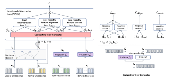
Figure 1. The structure overview of the proposed BM3. Projections $f_{v}$ and $f_{t}$, as well as predictor $f_{p}$, are all one-layer MLPs. The parameters of predictor $f_{p}$ are shared in the Contrastive View Generator (bottom left) for ID embeddings and multi-modal latent representations.

The structure overview of the proposed BM3.

3.1. Multi-modal Latent Space Convertor

Let $\mathbf{e}_{u},\mathbf{e}_{i}\in\mathbb{R}^{d}$ denote the input ID embeddings of the user $u\in\mathcal{U}$ and the item $i\in\mathcal{I}$, where $d$ is the embedding dimension, and $\mathcal{U},\mathcal{I}$ are the sets of users and items, respectively. Their cardinal numbers are set as $|\mathcal{U}|$ and $|\mathcal{I}|$, respectively. We denote the modality-specific features obtained from the pre-trained model as $\mathbf{e}_{m}\in\mathbb{R}^{d_{m}}$, where $m\in\mathcal{M}$ denotes a specific modality from the full set of modalities $\mathcal{M}$, and $d_{m}$ denotes the dimension of the features. The cardinal number of $\mathcal{M}$ is denoted by $|\mathcal{M}|$. In this paper, we consider two modalities: vision $v$ and text $t$. However, the model can be easily extended to scenarios with more than two modalities. As the multi-modal feature spaces are different from each other, we first convert the multi-modal features and ID embeddings into the same latent space.

3.1.1. Multi-modal Features

The features of an item obtained from different modalities are of different dimensions and in different feature spaces. For a multi-modal feature vector $\mathbf{e}_{m}$, we first project it into a latent low dimension using a projection function $f_{m}$ based on Multi-Layer Perceptron (MLP). Then, we have:

(1) $$\mathbf{h}_{m}=\mathbf{e}_{m}\mathbf{W}_{m}+\mathbf{b}_{m},$$

where $\mathbf{W}_{m}\in\mathbb{R}^{d_{m}\times d},\mathbf{b}_{m}\in\mathbb{R}^{d}$ denote the linear transformation matrix and bias in the MLP of $f_{m}$. In this way, each uni-modal latent representation $\mathbf{h}_{m}$ shares the same space with ID embeddings.

3.1.2. ID Embeddings

Previous work (Zhang et al., 2021) has verified the crucial role of ID embeddings in multi-modal recommendation. Although the ID embeddings of users and items can be directly initialized within the latent space, they do not encode any structural information about the user-item interaction graph. Inspired by the recent success of applying GCN for recommendation, we use a backbone network of LightGCN (He et al., 2020) with residual connection to encode the structure of the user-item interaction graph.

Suppose $\mathcal{G}=(\mathcal{V},\mathcal{E})$ be a given graph with node set $\mathcal{V}=\mathcal{U}\cup\mathcal{I}$ and edge set $\mathcal{E}$. The number of nodes is denoted by $|\mathcal{V}|$, and the number of edges is denoted by $|\mathcal{E}|$. The adjacency matrix is denoted by $\mathbf{A}\in\mathbb{R}^{|\mathcal{V}|\times|\mathcal{V}|}$, and the diagonal degree matrix is denoted by $\mathbf{D}$. In $\mathcal{G}$, the edges describe observed user-item interactions. If a user has interactions with an item, we build an edge between the user node and the item node. Moreover, we use $\mathbf{H}^{l}\in\mathbb{R}^{|\mathcal{V}|\times d}$ to denote the ID embeddings at the $l$-th layer by stacking all the embeddings of users and items at layer $l$. Specifically, the initial ID embeddings $\mathbf{H}^{0}$ is a collection of embeddings $\mathbf{e}_{u}$ and $\mathbf{e}_{i}$ from all users and items. A typical feed forward propagation GCN  (Kipf and Welling, 2017) to calculate the hidden ID embedding $\mathbf{H}^{l+1}$ at layer $l+1$ is recursively conducted as:

(2) $$\mathbf{H}^{l+1}=\sigma\left(\hat{\mathbf{A}}\mathbf{H}^{l}\mathbf{W}^{l}\right),$$

where $\sigma(\cdot)$ is a non-linear function, e.g., the ReLu function, $\hat{\mathbf{A}}=\hat{\mathbf{D}}^{-1/2}(\mathbf{A}+\mathbf{I})\hat{\mathbf{D}}^{-1/2}$ is the re-normalization of the adjacency matrix $\mathbf{A}$, and $\hat{\mathbf{D}}$ is the diagonal degree matrix of $\mathbf{A}+\mathbf{I}$. For node classification, the last layer of a GCN is used to predict the label of a node via a $softmax$ classifier.

On top of the vanilla GCN, LightGCN simplifies its structure by removing the feature transformation $\mathbf{W}^{l}$ and non-linear activation $\sigma(\cdot)$ layers for recommendation. As they found these two layers impose adverse effects on recommendation performance. The simplified graph convolutional layer in LightGCN is defined as:

(3) $$\mathbf{H}^{l+1}=(\mathbf{D}^{-1/2}\mathbf{A}\mathbf{D}^{-1/2})\mathbf{H}^{l},$$

where the node embeddings of the $(l+1)$-th hidden layer are only linearly aggregated from the $l$-th layer with a transition matrix $\mathbf{D}^{-1/2}\mathbf{A}\mathbf{D}^{-1/2}$. The transition matrix is exactly the weighted adjacency matrix mentioned above.

We use a readout function to aggregate all representations in hidden layers for user and item final representations. However, GCNs may suffer from the over-smoothing problem (Liu et al., 2020; Chen et al., 2020b; Li et al., 2021). Following LATTICE (Zhang et al., 2021), we also add a residual connection (Kipf and Welling, 2017; Chen et al., 2020b) to the item initial embeddings $\mathbf{H}^{0}_{i}$ to obtain the final representations of items. That is:

(4) $$\begin{split}\mathbf{H_{u}}&=\text{R{\scriptsize EADOUT}}(\mathbf{H}_{u}^{0},\mathbf{H}_{u}^{1},\mathbf{H}_{u}^{2},...,\mathbf{H}_{u}^{L});\\ \mathbf{H_{i}}&=\text{R{\scriptsize EADOUT}}(\mathbf{H}_{i}^{0},\mathbf{H}_{i}^{1},\mathbf{H}_{i}^{2},...,\mathbf{H}_{i}^{L})+\mathbf{H}^{0}_{i},\end{split}$$

where the READOUT function can be any differentiable function. We use the default mean function of LightGCN for its final ID embedding updating.

With the multi-modal latent space convertor, we can obtain three types of latent embeddings: user ID embeddings, item ID embeddings, and uni-modal item embeddings. In the following section, we illustrate the design of losses in BM3 for efficient parameter optimization without negative samples.

3.2. Multi-modal Contrastive Loss

Previous studies on SSL use the stop-gradient strategy to prevent the model from resulting in a trivial constant solution (Grill et al., 2020; Chen and He, 2021). Besides, they use online and target networks to make the model parameters learn in a teacher-student manner (Tarvainen and Valpola, 2017). BM3 simplifies the current SSL paradigm (Grill et al., 2020; Chen and He, 2021) by postponing the data augmentation after the encoding of the online network. We first illustrate the data augmentation in BM3.

Table 1. Comparison of computational complexity on graph-based multi-modal methods.

Component	MMGCN	GRCN	DualGNN	LATTICE	BM3
Graph Convolution	$\mathcal{O}(|\mathcal{M}|X)$	$\mathcal{O}((|\mathcal{M}|+1)X)$	$\mathcal{O}(|\mathcal{M}|X+kd|\mathcal{U}|)$	$\mathcal{O}(X)$	$\mathcal{O}(X)$
Feature Transform	$\mathcal{O}(\displaystyle\sum_{m\in\mathcal{M}}|\mathcal{I}|(d_{m}+d)d_{h})$	$\mathcal{O}(\displaystyle\sum_{m\in\mathcal{M}}|\mathcal{I}|d_{m}d)$	$\mathcal{O}(\displaystyle\sum_{m\in\mathcal{M}}|\mathcal{I}|(d_{m}+d)d_{h})$	$\mathcal{O}(|\mathcal{I}|^{3}+\displaystyle\sum_{m\in\mathcal{M}}|\mathcal{I}|^{2}d_{m}$ $+k|\mathcal{I}|\log(|\mathcal{I}|))$	$\mathcal{O}(\displaystyle\sum_{m\in\mathcal{M}}|\mathcal{I}|d_{m}d)$
BPR/CL Losses	$\mathcal{O}(2dB)$	$\mathcal{O}((2+|\mathcal{M}|)dB)$	$\mathcal{O}((2+|\mathcal{M}|)dB)$	$\mathcal{O}(2dB)$	$\mathcal{O}((2+2|\mathcal{M}|)dB)$
To fit the page, we set $X=2L|\mathcal{E}|d/B$, and $d_{h}$ denotes the dimension of the hidden layer in a two-layer MLP.

3.2.1. Contrastive View Generator

Prior studies (Lee et al., 2021; Wu et al., 2021b; Thakoor et al., 2021) use graph augmentations to generate two alternate views of the original graph for self-supervised learning. Input features are encoded through both graphs to generate the contrastive views. To reduce the computational complexity and the memory cost, BM3 removes the requirement of graph augmentations with a simple latent embedding dropout technique that is analogous to node dropout (Srivastava et al., 2014). The contrastive latent embedding $\dot{\mathbf{h}}$ of $\mathbf{h}$ under a dropout ratio $p$ is calculated as:

(5) $$\dot{\mathbf{h}}=\mathbf{h}\cdot\text{Bernoulli}(p).$$

Following (Grill et al., 2020; Chen and He, 2021), we also place stop-gradient on the contrastive view $\dot{\mathbf{h}}$. Whilst we feed the original embedding $\mathbf{h}$ into a predictor of MLP.

(6) $$\tilde{\mathbf{h}}=\mathbf{h}\mathbf{W}_{p}+\mathbf{b}_{p},$$

where $\mathbf{W}_{p}\in\mathbb{R}^{d\times d},\mathbf{b}_{p}\in\mathbb{R}^{d}$ denote the linear transformation matrix and bias in the predictor function $f_{p}$.

3.2.2. Graph Reconstruction Loss

BM3 takes a positive user-item pair $(u,i)$ as input. With the generated contrastive view $(\dot{\mathbf{h}}_{u},\dot{\mathbf{h}}_{i})$ of the online representations $(\tilde{\mathbf{h}}_{u},\tilde{\mathbf{h}}_{i})$, we define a symmetrized loss function as the negative cosine similarity between $(\tilde{\mathbf{h}}_{u},\dot{\mathbf{h}}_{i})$ and $(\dot{\mathbf{h}}_{u},\tilde{\mathbf{h}}_{i})$:

(7) $$\mathcal{L}_{rec}=\mathcal{C}(\tilde{\mathbf{h}}_{u},\dot{\mathbf{h}}_{i})+\mathcal{C}(\dot{\mathbf{h}}_{u},\tilde{\mathbf{h}}_{i}).$$

Function $\mathcal{C}(\cdot,\cdot)$ in the above equation is defined as:

(8) $$\mathcal{C}(\mathbf{h}_{u},\mathbf{h}_{i})=-\frac{\mathbf{h}_{u}^{T}\mathbf{h}_{i}}{||\mathbf{h}_{u}||_{2}||\mathbf{h}_{i}||_{2}},$$

where $||\cdot||_{2}$ is $\ell_{2}$-norm. The total loss is averaged over all user-item pairs. The intuition behind this is that we intend to maximize the prediction of the positively perturbed item $i$ given a user $u$, and vice versa. The minimized possible value for this loss is $-1$.

Finally, we stop gradient on the target network and force the backpropagation of loss over the online network only. We follow the stop gradient ($sg$) operator as in (Grill et al., 2020; Chen and He, 2021), and implement the operator by updating Eq. (7) as:

(9) $$\mathcal{L}_{rec}=\mathcal{C}(\tilde{\mathbf{h}}_{u},sg(\dot{\mathbf{h}}_{i}))+\mathcal{C}(sg(\dot{\mathbf{h}}_{u}),\tilde{\mathbf{h}}_{i}).$$

With the stop gradient operator, the target network receives no gradient from $(\dot{\mathbf{h}}_{u},\dot{\mathbf{h}}_{i})$.

3.2.3. Inter-modality Feature Alignment Loss

In addition, we further align the multi-modal features of items with their target ID embeddings. The alignment encourages the ID embeddings close to each other on items with similar multi-modal features. For each uni-modal latent embedding $\mathbf{h}_{m}$ of an item $i$, the contrastive view generator outputs its contrastive pair as $(\tilde{\mathbf{h}}_{m}^{i},\dot{\mathbf{h}}_{m}^{i})$. We use the negative cosine similarity to perform the alignment between $\dot{\mathbf{h}}_{i}$ and $\tilde{\mathbf{h}}_{m}^{i}$:

(10) $$\mathcal{L}_{align}=\mathcal{C}(\tilde{\mathbf{h}}_{m}^{i},\dot{\mathbf{h}}_{i}).$$

3.2.4. Intra-modality Feature Masked Loss

Finally, BM3 uses intra-modlity feature masked loss to further encourage the learning of predictor with sparse representations of latent embeddings. Sparse is verified scale efficient in large transformers (Jaszczur et al., 2021; Shi et al., 2022). We randomly mask out a subset of the latent embedding $\mathbf{h}_{m}$ by dropout with the contrastive view generator and denote the sparse embedding as $\dot{\mathbf{h}}_{m}^{i}$. The intra-modality feature masked loss is defined as:

(11) $$\mathcal{L}_{mask}=\mathcal{C}(\tilde{\mathbf{h}}_{m}^{i},\dot{\mathbf{h}}_{m}^{i}).$$

Additionally, we add regularization penalty on the online embeddings (i.e., $\mathbf{h}_{u}$ and $\mathbf{h}_{i}$). Our final loss function is:

(12) $$\mathcal{L}=\mathcal{L}_{rec}+\mathcal{L}_{align}+\mathcal{L}_{mask}+\lambda\cdot(||\mathbf{h}_{u}||^{2}_{2}+||\mathbf{h}_{i}||^{2}_{2}).$$

3.3. Top-$K$ Recommendation

To generate item recommendations for a user, we first predict the interaction scores between the user and candidate items. Then, we rank candidate items based on the predicted interaction scores in descending order, and choose $K$ top-ranked items as recommendations to the user. Classical CF methods recommend top-$K$ items by ranking scores of the inner product of a user embedding with all candidate item embeddings. As our MMCL can learn a good predictor on user and item latent embeddings, we use the embeddings transformed by the predictor $f_{p}$ for inner product. That is:

(13) $$s(\mathbf{h}_{u},\mathbf{h}_{i})=\tilde{\mathbf{h}}_{u}\cdot\tilde{\mathbf{h}}_{i}^{T}.$$

A high score suggests that the user prefers the item.

3.4. Computational Complexity

The computational cost of BM3 mainly occurs in linear propagation of the normalized adjacency matrix $\hat{\mathbf{A}}$. The analytical complexity of LightGCN and BM3 are in the same magnitude with $\mathcal{O}(2L|\mathcal{E}|d/B)$ on graph convolutional operation, where $L$ is the number of LightGCN layers, and $B$ is the training batch size. However, BM3 has additional costs on multi-modal feature projection and prediction. The projection cost is $\mathcal{O}(\sum_{m\in\mathcal{M}}|\mathcal{I}|d_{m}d)$ on all modalities. The contrastive loss cost is $\mathcal{O}((2+2|\mathcal{M}|)dB)$. The total computational cost for BM3 is $\mathcal{O}(2L|\mathcal{E}|d/B+\sum_{m\in\mathcal{M}}|\mathcal{I}|d_{m}d+(2+2|\mathcal{M}|)dB)$. We summarize the computational complexity of the graph-based multi-modal methods in Table 1. Both MMGCN and DualGNN use a two-layer MLP for multi-modal feature projection. On the contrary, LATTICE constructs an item-item graph from the multi-modal features. It costs $\mathcal{O}(|\mathcal{I}|^{2}d_{m})$ to build the similarity matrix between items, $\mathcal{O}(|\mathcal{I}|^{3})$ to normalize the matrix, and $\mathcal{O}(k|\mathcal{I}|\log(|\mathcal{I}|))$ to retrieve top-$k$ most similar items for each item.

Table 2. Statistics of the experimental datasets.

Datasets	# Users	# Items	# Interactions	Sparsity
Baby	19,445	7,050	160,792	99.88%
Sports	35,598	18,357	296,337	99.95%
Electronics	192,403	63,001	1,689,188	99.99%

4. Experiments

We perform comprehensive experiments to evaluate the effectiveness and efficiency of BM3 to answer the following research questions.

• RQ1: Can the self-supervised model leveraging only positive user-item interactions outperform or match the performance of the supervised baselines?

• RQ2: How efficient of the proposed BM3 model in multi-modal recommendation with regard to the computational complexity and memory cost?

• RQ3: To what extent the multi-modal features could affect the recommendation performance of BM3?

• RQ4: How different losses in BM3 affect its recommendation accuracy?

4.1. Experimental Datasets

Following previous studies (He and McAuley, 2016b; Zhang et al., 2021), we use the Amazon review dataset (He and McAuley, 2016a) for experimental evaluation. This dataset provides both product descriptions and images simultaneously, and it is publicly available and varies in size under different product categories. To ensure as many baselines can be evaluated on large-scale datasets, we choose three per-category datasets, i.e., Baby, Sports and Outdoors (denoted by Sports), and Electronics, for performance evaluation . In these datasets, each review rating is treated as a record of positive user-item interaction. This setting has been widely used in previous studies (He and McAuley, 2016b; Zhang et al., 2021; He et al., 2020; Zhang et al., 2022). The raw data of each dataset are pre-processed with a 5-core setting on both items and users, and their 5-core filtered results are presented in Table 2, where the data sparsity is measured as the number of interactions divided by the product of the number of users and the number of items. The pre-processed datasets include both visual and textual modalities. Following (Zhang et al., 2021), we use the 4,096-dimensional visual features that have been extracted and published in (Ni et al., 2019). For the textual modality, we extract textual embeddings by concatenating the title, descriptions, categories, and brand of each item and utilize sentence-transformers (Reimers and Gurevych, 2019) to obtain 384-dimensional sentence embeddings.

Table 3. Overall performance achieved by different recommendation methods in terms of Recall and NDCG. We mark the global best results on each dataset under each metric in boldface and the second best is underlined.

Datasets	Metrics	General models			Multi-modal models
		BPR	LightGCN	BUIR	VBPR	MMGCN	GRCN	DualGNN	LATTICE	BM3
Baby	R@10	0.0357	0.0479	0.0506	0.0423	0.0378	0.0532	0.0448	0.0544	0.0564
	R@20	0.0575	0.0754	0.0788	0.0663	0.0615	0.0824	0.0716	0.0848	0.0883
	N@10	0.0192	0.0257	0.0269	0.0223	0.0200	0.0282	0.0240	0.0291	0.0301
	N@20	0.0249	0.0328	0.0342	0.0284	0.0261	0.0358	0.0309	0.0369	0.0383
Sports	R@10	0.0432	0.0569	0.0467	0.0558	0.0370	0.0559	0.0568	0.0618	0.0656
	R@20	0.0653	0.0864	0.0733	0.0856	0.0605	0.0877	0.0859	0.0947	0.0980
	N@10	0.0241	0.0311	0.0260	0.0307	0.0193	0.0306	0.0310	0.0337	0.0355
	N@20	0.0298	0.0387	0.0329	0.0384	0.0254	0.0389	0.0385	0.0422	0.0438
Electronics	R@10	0.0235	0.0363	0.0332	0.0293	0.0207	0.0349	0.0363	-	0.0437
	R@20	0.0367	0.0540	0.0514	0.0458	0.0331	0.0529	0.0541	-	0.0648
	N@10	0.0127	0.0204	0.0185	0.0159	0.0109	0.0195	0.0202	-	0.0247
	N@20	0.0161	0.0250	0.0232	0.0202	0.0141	0.0241	0.0248	-	0.0302
‘-’ indicates the model cannot be fitted into a Tesla V100 GPU card with 32 GB memory.

4.2. Baseline Methods

To demonstrate the effectiveness of BM3, we compare it with the following state-of-the-art recommendation methods, including general CF recommendation models and multi-modal recommendation models.

• BPR (Rendle et al., 2009): This is a matrix factorization model optimized by a pair-wise ranking loss in a Bayesian way.

• LightGCN (He et al., 2020): This is a simplified graph convolution network that only performs linear propagation and aggregation between neighbors. The hidden layer embeddings are averaged to calculate the final user and item embeddings for prediction.

• BUIR (Lee et al., 2021): This self-supervised framework uses asymmetric network architecture to update its backbone network parameters. In BUIR, LightGCN is used as the backbone network. It is worth noting that BUIR does not rely on negative samples for learning.

• VBPR (He and McAuley, 2016b): This model incorporates visual features for user preference learning with BPR loss. Following (Zhang et al., 2021; Wang et al., 2021b), we concatenate the multi-modal features of an item as its visual feature for user preference learning.

• MMGCN (Wei et al., 2019): This method constructs a modal-specific graph to learn user preference on each modality leveraging GCN. The final user and item representations are generated by combining the learned representations from each modality.

• GRCN (Wei et al., 2020): This method improves previous GCN-based models by refining the user-item bipartite graph with removal of false-positive edges. User and item representations are learned on the refined bipartite graph by performing information propagation and aggregation.

• DualGNN (Wang et al., 2021b): This method builds an additional user-user correlation graph from the user-item bipartite graph and uses it to fuse the user representation from its neighbors in the correlation graph.

• LATTICE (Zhang et al., 2021): This method mines the latent structure between items by learning an item-item graph from their multi-modal features. Graph convolutional operations are performed on both item-item graph and user-item interaction graph to learn user and item representations.

We group the first three baselines (i.e., BPR, LightGCN, and BUIR) as general models, because they only use implicit feedback (i.e., user-item interactions) for recommendation. The other multi-modal models utilize both implicit feedback and multi-modal features for recommendation. Analogously, we categorize BUIR into the self-supervised model and the others as supervised models as they are using negative samples for representation learning. The proposed BM3 model is within the self-supervised multi-modal domain.

4.3. Setup and Evaluation Metrics

For a fair comparison, we follow the same evaluation setting of (Zhang et al., 2021; Wang et al., 2021b) with a random data splitting 8:1:1 on the interaction history of each user for training, validation and testing. Moreover, we use $\text{Recall}@K$ and $\text{NDCG}@K$ to evaluate the top-$K$ recommendation performance of different recommendation methods. Specifically, we use the all-ranking protocol instead of the negative-sampling protocol to compute the evaluation metrics for recommendation accuracy comparison. In the recommendation phase, all items that have not been interacted by the given user are regarded as candidate items. In the experiments, we empirically report the results of $K$ at 10, 20 and abbreviate the metrics of $\text{Recall}@K$ and $\text{NDCG}@K$ as $\text{R}@K$ and $\text{N}@K$, respectively.

4.4. Implementation Details

Same as other existing work (He et al., 2020; Zhang et al., 2021), we fix the embedding size of both users and items to 64 for all models, initialize the embedding parameters with the Xavier method (Glorot and Bengio, 2010), and use Adam (Kingma and Ba, 2015) as the optimizer with a learning rate of 0.001. For a fair comparison, we carefully tune the parameters of each model following their published papers. The proposed BM3 model is implemented by PyTorch (Paszke et al., 2019). We perform a grid search across all datasets to conform to its optimal settings. Specifically, the number of GCN layers is tuned in {1, 2}. The dropout rate for embedding perturbation is chosen from {0.3, 0.5}, and the regularization coefficient is searched in {0.1, 0.01}. For convergence consideration, the early stopping and total epochs are fixed at 20 and 1000, respectively. Following (Zhang et al., 2021), we use R@20 on the validation data as the training stopping indicator. We have integrated our model and all baselines into the unified multi-modal recommendation platform, MMRec (Zhou, 2023).

Table 4. Efficiency comparison of BM3 against the baselines.

Datasets	Metrics	General models			Multi-modal models
		BPR	LightGCN	BUIR	VBPR	MMGCN	GRCN	DualGNN*	LATTICE	BM3
Baby	Memory (GB)	1.59	1.69	2.29	1.89	2.69	2.95	2.05	4.53	2.11
	Time ($s$/epoch)	0.47	0.99	0.77	0.57	3.48	2.36	7.81	1.61	0.85
Sports	Memory (GB)	2.00	2.24	3.75	2.71	3.91	4.49	2.81	19.93	3.58
	Time ($s$/epoch)	0.95	2.86	2.19	1.28	16.60	6.74	12.60	10.71	3.03
Electronics	Memory (GB)	3.69	4.92	10.13	6.20	14.54	17.38	8.85	-	8.28
	Time ($s$/epoch)	6.75	67.49	63.77	14.20	470.15	152.68	341.02	-	73.31
‘-’ denotes the model cannot be fitted into a Tesla V100 GPU card with 32 GB memory.
‘*’ In pre-processing, DualGNN requires about 138GB memory and 6 hours to construct the user-user relationship graph on Electronics data.

4.5. Effectiveness of BM3 (RQ1)

The performance achieved by different recommendation methods on all three datasets are summarized in Table 3. From the table, we have the following observations. First, the proposed BM3 model significantly outperforms both general recommendation methods and state-of-the-art multi-modal recommendation methods on each dataset. Specifically, BM3 improves the best baselines by 3.68%, 6.15%, and 20.39% in terms of Recall@10 on Baby, Sports, and Electronics, respectively. The results not only verify the effectiveness of BM3 in recommendation, but also show BM3 is superior to the baselines for recommendation on the large graph (i.e., Electronics). Second, multi-modal recommendation models do not always outperform the general recommendation models without leveraging modal features. Although the recommendation accuracy of VBPR building upon BPR dominates its counterpart (i.e., BPR) across all datasets, GRCN and DualGNN using LightGCN as its downstream CF model do not gain much improvement over LightGCN. Differing from the multi-modal feature fusion mechanism of MMGCN, GRCN, and DualGNN, LATTICE uses the multi-modal features in an indirect manner by building an item-item relation graph and performs graph convolutional operation on the graph. We speculate there are two potential reasons leading to the suboptimal performance of MMGCN, GRCN, and DualGNN. i). They fuse the item ID embedding with its modal-specific features. Table 3 shows that LightGCN with ID embeddings can obtain good recommendation accuracy. The mixing of ID embeddings and modal features causes the items to lose their identities in recommendation, resulting in accuracy degradation. ii). They fail to differentiate the importance of multi-modal features of items. In MMGCN, GRCN, and DualGNN, they treat features from each modality equally. However, our ablation study in Section 4.7 shows that the extracted visual features may contain noise and are less informative than the textual features. On the contrary, LATTICE learns the weights between multi-modal features when building the item-item graph. The proposed BM3 model alleviates the above issues by placing the contributions of multi-modal features into the loss function. Finally, we compare the recommendation accuracy between self-supervised learning models (i.e., BUIR and BM3). Although BUIR shows comparable performance with LightGCN, it is inferior to BM3. The performance of BUIR depends on the perturbed graph. Better contrastive view results in better recommendation acrruacy. As a result, it obtains fluctuating performance over different datasets. BM3 reduces the requirement of graph augmentation by latent embedding dropout. It is earlier for BM3 to obtain a consistent contrastive view with the original view than BUIR. Moreover, BM3 is more efficient than BUIR, because it uses only one backbone network.

4.6. Efficiency of BM3 (RQ2)

Apart from the comparison of recommendation accuracy, we also report the efficiency of BM3 against the baselines, in terms of utilized memory and training time per epoch. It is worth noting that all models are firstly evaluated on a GeForce RTX 2080 Ti with 12GB memory, and the model will be advanced to a Tesla V100 GPU with 32 GB memory if it cannot be fitted into the 12 GB memory. The efficiencies of different methods are summarized in Table 4. From the table, we can have the following two observations. First, from both the general model and multi-modal model perspectives, graph-based models usually consume more memory than classic CF models (i.e., BPR and VBPR). Specifically, classic CF models require a minimum GPU memory cost for representation learning of users and items. Whilst graph-based models usually need to retain an additional user-item interaction graph for information propagation and aggregation. Moreover, graph-based multi-modal recommendation models need more memory, as they use both the user-item graph and multi-modal features in general. Second, among the graph-based multi-modal recommendation models, BM3 consumes less or comparable memory than other baselines. However, it reduces the training time by 2–9$\times$ per epoch. Compared with the best baseline, BM3 requires only half of the training time and half of the consumed memory of LATTICE. Although BM3 uses LightGCN as its backbone model, it does not introduce much additional cost on LightGCN other than the multi-modal features. The reason is that BM3 removes the negative sampling time and uses fewer GCN layers.

Table 5. Ablation study of BM3 on multi-modal features.

Datasets	Variants	R@10	R@20	N@10	N@20
Baby	BM3w/o v&t	0.0506	0.0793	0.0273	0.0347
	BM3w/o t	0.0518	0.0820	0.0277	0.0354
	BM3w/o v	0.0522	0.0828	0.0279	0.0358
	BM3	0.0564	0.0883	0.0301	0.0383
Sports	BM3w/o v&t	0.0600	0.0927	0.0326	0.0410
	BM3w/o t	0.0641	0.0976	0.0349	0.0435
	BM3w/o v	0.0647	0.0968	0.0349	0.0432
	BM3	0.0656	0.0980	0.0355	0.0438
Elec.	BM3w/o v&t	0.0427	0.0633	0.0240	0.0293
	BM3w/o t	0.0423	0.0632	0.0237	0.0291
	BM3w/o v	0.0423	0.0633	0.0236	0.0290
	BM3	0.0437	0.0648	0.0247	0.0302

4.7. Ablation Study (RQ3 & RQ4)

To fully understand the behaviors of BM3, we perform ablation studies on both the multi-modal features and different parts of the multi-modal contrastive loss.

4.7.1. Multi-modal Features (RQ3)

We evaluate the recommendation accuracy of BM3 by feeding individual modal features into the model. Specifically, we design the following variants of BM3.

• BM3_{w/o v&t}: In this variant, BM3 degrades to a general recommendation model that exploits only the user-item interactions for recommendation.

• BM3_{w/o v}: This variant of BM3 learns the representations of users and items without the visual features of items.

• BM3_{w/o t}: This variant of BM3 is trained without the input from the textual features.

Table 5 summarizes the recommendation performance of BM3 and its variants, i.e., BM3_{w/o v&t}, BM3_{w/o v}, and BM3_{w/o t}, on all three experimental datasets.

As shown in Table 5, the importance of textual and visual features varies with datasets. BM3_{w/o v} leveraging only on the textual features gains slight better recommendation accuracy than BM3_{w/o t} on Baby dataset. However, on the other datasets, the differences between these two variations are negligible. Moreover, we can observe that the context features from either textual or visual modality can boost the performance of BM3_{w/o v&t} on Baby and Sports datasets. However, this statement does not hold under the large dataset, i.e., Electronics. By combining both the textual and visual features, BM3 achieves the best recommendation accuracy on all three datasets.

Comparing the experimental results in Table 5 with that in Table 3, we note that BM3_{w/o v&t} without any multi-modal features is competitive with most multi-modal baseline models and superior to the general baseline models. This demonstrates the effectiveness of the self-supervised learning paradigm for top-$K$ item recommendation. It is worth noting that BM3 uses LightGCN as its backbone network. The best performance of BM3 is achieved by using 1, 1, and 2 GCN layers on Baby, Sports, and Electronics datasets, respectively. Whilst LightGCN itself requires 4 GCN layers to achieve its best performance on all datasets.

Table 6. Ablation study on different parts of the multi-modal contrastive loss of BM3.

Datasets	Variants	R@10	R@20	N@10	N@20
Baby	BM3w/o mm	0.0506	0.0793	0.0273	0.0347
	BM3w/o inter	0.0542	0.0842	0.0289	0.0366
	BM3w/o intra	0.0526	0.0830	0.0281	0.0360
	BM3	0.0564	0.0883	0.0301	0.0383
Sports	BM3w/o mm	0.0600	0.0927	0.0326	0.0410
	BM3w/o inter	0.0614	0.0941	0.0336	0.0420
	BM3w/o intra	0.0633	0.0947	0.0344	0.0425
	BM3	0.0656	0.0980	0.0355	0.0438
Elec.	BM3w/o mm	0.0427	0.0633	0.0240	0.0293
	BM3w/o inter	0.0393	0.0593	0.0218	0.0270
	BM3w/o intra	0.0410	0.0619	0.0227	0.0281
	BM3	0.0437	0.0648	0.0247	0.0302

4.7.2. Multi-modal Contrastive Loss (RQ4)

As the loss function plays a critical role in learning the model parameters of BM3 without negative samples. We further study the behaviors of BM3 by removing different parts of the multi-modal contrastive loss. Specifically, we consider the following variants of BM3 for experimental evaluation.

• BM3_{w/o mm}: This variant only uses the interaction graph reconstruction loss to train the model parameters, i.e., trained without the multi-modal losses. It is worth noting that this variant is equivalent to BM3_{w/o v&t}.

• BM3_{w/o inter}: In this variant, the representations of users and items are learned without considering the inter-modality alignment loss.

• BM3_{w/o intra}: This variant learns the representations of users and items without considering the feature masked loss.

Table 6 shows the performance achieved by BM3, BM3_{w/o mm}, BM3_{w/o inter}, and BM3_{w/o intra} on all three datasets.

From Table 6, we find a similar pattern as that shown in the ablation study on multi-modal features. That is, the multi-modal losses can improve the recommendation accuracy of BM3 on Baby and Sports datasets. However, BM3 leveraging either the inter-modality alignment loss or the intra-modality feature masked loss degrades its performance on the Electronics dataset. Moreover, the importance of inter- and intra-modality losses also varies with the datasets.

From the ablation studies on features and the loss function, we find the recommendation accuracy on the large dataset (i.e., Electronics) shows a different pattern from that of the small-scale datasets (i.e., Baby and Sports). The uni-modal feature or uni-loss function in BM3 shows no improvement in recommendation accuracy on Electronics dataset. We speculate that the supervised or self-supervised signals on a large dataset already enable BM3_{w/o mm} to learn good representations of users and items. Adding coarse multi-modal signals to BM3_{w/o mm} does not help improve the recommendation accuracy.

5. Conclusion

This paper proposes a novel self-supervised learning framework, named BM3, for multi-modal recommendation. BM3 removes the requirement of randomly sampled negative examples in modeling the interactions between users and items. To generate a contrastive view in self-supervised learning, BM3 utilizes a simple yet efficient latent embedding dropout mechanism to perturb the original embeddings of users and items. Moreover, a novel learning paradigm based on the multi-modal contrastive loss has also been devised. Specifically, the contrastive loss jointly minimizes: a) the reconstruction loss of the user-item interaction graph, b) the alignment loss between ID embeddings of items and their multi-modal features, and c) the masked loss within a modality-specific feature. We evaluate the proposed BM3 model on three real-world datasets, including one large-scale dataset, to demonstrate its effectiveness and efficiency in recommendation tasks. The experimental results show that BM3 achieves significant accuracy improvements over the state-of-the-art multi-modal recommendation methods, while training 2-9$\times$ faster than the baseline methods.

6. Appendices

6.1. Hyper-parameter Sensitivity Study

To guide the selection of hyper-parameters of BM3, we perform a hyper-parameter sensitivity study with regard to the recommendation accuracy, in terms of Recall@20. We use at least two datasets to evaluate the performance of BM3 under different hyper-parameter settings. Specifically, we consider the following three hyper-parameters, i.e., the number of GCN layers $L$, the ratio of embedding dropout, and the regularization coefficient factor $\lambda$.

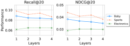
Figure 2. Top-20 recommendation accuracy of BM3 varies with the number of GCN layers in the backbone network.

Top-20 recommendation accuracy of BM3 varies with the number of GCN layers in the backbone network.

6.1.1. The Number of GCN Layers

The number of GCN layers $L$ in BM3 is varied in {1, 2, 3, 4}. Fig. 2 shows the performance trends of BM3 with respect to different settings of $L$. As shown in Fig. 2, BM3 shows relatively slow performance degradation as the number of layers increases, on small-scale datasets (i.e., Baby and Sports). However, the recommendation accuracy can be improved with more than one GCN layer in the backbone network on Electronics dataset.

6.1.2. The Dropout Ratio and Regularization Coefficient

We vary the dropout ratio of BM3 from 0.1 to 0.5 with a step of 0.1, and vary the regularization coefficient $\lambda$ in {0.0001, 0.001, 0.01, 0.1}. Fig. 3b shows the performance achieved by BM3 under different combinations of the embedding dropout ratio and regularization coefficient. We note that a larger dropout ratio of BM3 on a relative small-scale dataset (i.e., Sports) usually helps BM3 achieve better recommendation accuracy. Moroever, the performance of BM3 is less sensitive to the settings of regularization coefficient on the large dataset (i.e., Electronics). In Fig. 3b(b), it is worth noting that BM3 achieves competitive recommendation accuracy when the dropout ratio is larger than 0.2. This verifies the stability of BM3 in the recommendation task, i.e., the recommendation performance of BM3 is not just a consequence of random seeds.

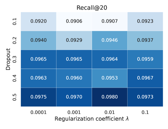
(a) Sports

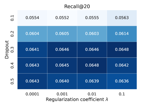
(b) Electronics

Figure 3. The Performance achieved by BM3 with respect to different combinations of the latent embedding dropout ratio and regularization coefficient on three datasets. Darker background indicates better recommendation accuracy.

The Performance achieved by BM3 with respect to different combinations of the latent embedding dropout ratio and regularization coefficient on three datasets. Darker background indicates better recommendation accuracy.

References

- (1)
- Bromley et al. (1993) Jane Bromley, Isabelle Guyon, Yann LeCun, Eduard Säckinger, and Roopak Shah. 1993. Signature verification using a” siamese” time delay neural network. Advances in neural information processing systems 6 (1993), 737–744.
- Chen et al. (2020b) Ming Chen, Zhewei Wei, Zengfeng Huang, Bolin Ding, and Yaliang Li. 2020b. Simple and deep graph convolutional networks. In International Conference on Machine Learning. PMLR, 1725–1735.
- Chen et al. (2020a) Ting Chen, Simon Kornblith, Mohammad Norouzi, and Geoffrey Hinton. 2020a. A simple framework for contrastive learning of visual representations. In International Conference on Machine Learning. 1597–1607.
- Chen et al. (2019) Xu Chen, Hanxiong Chen, Hongteng Xu, Yongfeng Zhang, Yixin Cao, Zheng Qin, and Hongyuan Zha. 2019. Personalized fashion recommendation with visual explanations based on multimodal attention network: Towards visually explainable recommendation. In Proceedings of the 42nd International ACM SIGIR Conference on Research and Development in Information Retrieval. 765–774.
- Chen and He (2021) Xinlei Chen and Kaiming He. 2021. Exploring Simple Siamese Representation Learning. In Proceedings of the IEEE Conference on Computer Vision and Pattern Recognition. IEEE.
- Glorot and Bengio (2010) Xavier Glorot and Yoshua Bengio. 2010. Understanding the difficulty of training deep feedforward neural networks. In Proceedings of the thirteenth international conference on artificial intelligence and statistics. JMLR Workshop and Conference Proceedings, 249–256.
- Grill et al. (2020) Jean-Bastien Grill, Florian Strub, Florent Altché, Corentin Tallec, Pierre H Richemond, Elena Buchatskaya, Carl Doersch, Bernardo Avila Pires, Zhaohan Daniel Guo, Mohammad Gheshlaghi Azar, et al. 2020. Bootstrap your own latent: A new approach to self-supervised learning. In Proceedings of the 34th Annual Conference on Neural Information Processing Systems. 21271–21284.
- He and McAuley (2016a) Ruining He and Julian McAuley. 2016a. Ups and downs: Modeling the visual evolution of fashion trends with one-class collaborative filtering. In proceedings of the 25th international conference on world wide web. 507–517.
- He and McAuley (2016b) Ruining He and Julian McAuley. 2016b. VBPR: visual bayesian personalized ranking from implicit feedback. In Proceedings of the AAAI conference on artificial intelligence, Vol. 30.
- He et al. (2020) Xiangnan He, Kuan Deng, Xiang Wang, Yan Li, Yongdong Zhang, and Meng Wang. 2020. Lightgcn: Simplifying and powering graph convolution network for recommendation. In Proceedings of the 43rd International ACM SIGIR Conference on Research and Development in Information Retrieval. 639–648.
- Jaszczur et al. (2021) Sebastian Jaszczur, Aakanksha Chowdhery, Afroz Mohiuddin, Lukasz Kaiser, Wojciech Gajewski, Henryk Michalewski, and Jonni Kanerva. 2021. Sparse is enough in scaling transformers. Advances in Neural Information Processing Systems 34 (2021), 9895–9907.
- Jing and Tian (2020) Longlong Jing and Yingli Tian. 2020. Self-supervised visual feature learning with deep neural networks: A survey. IEEE transactions on pattern analysis and machine intelligence 43, 11 (2020), 4037–4058.
- Kingma and Ba (2015) Diederik P Kingma and Jimmy Ba. 2015. Adam: A method for stochastic optimization. In International Conference on Learning Representations.
- Kipf and Welling (2017) Thomas N Kipf and Max Welling. 2017. Semi-supervised classification with graph convolutional networks. In International Conference on Learning Representations.
- Lee et al. (2021) Dongha Lee, SeongKu Kang, Hyunjun Ju, Chanyoung Park, and Hwanjo Yu. 2021. Bootstrapping User and Item Representations for One-Class Collaborative Filtering. In Proceedings of the 44th International ACM SIGIR Conference on Research and Development in Information Retrieval.
- Li et al. (2021) Guohao Li, Matthias Müller, Bernard Ghanem, and Vladlen Koltun. 2021. Training graph neural networks with 1000 layers. In International conference on machine learning. PMLR, 6437–6449.
- Liu et al. (2019) Fan Liu, Zhiyong Cheng, Changchang Sun, Yinglong Wang, Liqiang Nie, and Mohan Kankanhalli. 2019. User diverse preference modeling by multimodal attentive metric learning. In Proceedings of the 27th ACM international conference on multimedia. 1526–1534.
- Liu et al. (2020) Meng Liu, Hongyang Gao, and Shuiwang Ji. 2020. Towards deeper graph neural networks. In Proceedings of the 26th ACM SIGKDD international conference on knowledge discovery & data mining. 338–348.
- Liu et al. (2017) Qiang Liu, Shu Wu, and Liang Wang. 2017. Deepstyle: Learning user preferences for visual recommendation. In Proceedings of the 40th international acm sigir conference on research and development in information retrieval. 841–844.
- Liu et al. (2021) Xiao Liu, Fanjin Zhang, Zhenyu Hou, Li Mian, Zhaoyu Wang, Jing Zhang, and Jie Tang. 2021. Self-supervised learning: Generative or contrastive. IEEE Transactions on Knowledge and Data Engineering (2021).
- Ni et al. (2019) Jianmo Ni, Jiacheng Li, and Julian McAuley. 2019. Justifying recommendations using distantly-labeled reviews and fine-grained aspects. In Proceedings of the 2019 Conference on Empirical Methods in Natural Language Processing and the 9th International Joint Conference on Natural Language Processing (EMNLP-IJCNLP). 188–197.
- Paszke et al. (2019) Adam Paszke, Sam Gross, Francisco Massa, Adam Lerer, James Bradbury, Gregory Chanan, Trevor Killeen, Zeming Lin, Natalia Gimelshein, Luca Antiga, et al. 2019. Pytorch: An imperative style, high-performance deep learning library. Advances in neural information processing systems 32 (2019).
- Reimers and Gurevych (2019) Nils Reimers and Iryna Gurevych. 2019. Sentence-bert: Sentence embeddings using siamese bert-networks. In EMNLP. 3980–3990.
- Rendle et al. (2009) Steffen Rendle, Christoph Freudenthaler, Zeno Gantner, and Lars Schmidt-Thieme. 2009. BPR: Bayesian Personalized Ranking from Implicit Feedback. In Proceedings of the Twenty-Fifth Conference on Uncertainty in Artificial Intelligence. 452–461.
- Shi et al. (2022) Baifeng Shi, Yale Song, Neel Joshi, Trevor Darrell, and Xin Wang. 2022. Visual Attention Emerges from Recurrent Sparse Reconstruction. arXiv preprint arXiv:2204.10962 (2022).
- Shorten and Khoshgoftaar (2019) Connor Shorten and Taghi M Khoshgoftaar. 2019. A survey on image data augmentation for deep learning. Journal of Big Data 6, 1 (2019), 1–48.
- Simonyan and Zisserman (2014) Karen Simonyan and Andrew Zisserman. 2014. Very deep convolutional networks for large-scale image recognition. arXiv preprint arXiv:1409.1556 (2014).
- Srivastava et al. (2014) Nitish Srivastava, Geoffrey Hinton, Alex Krizhevsky, Ilya Sutskever, and Ruslan Salakhutdinov. 2014. Dropout: a simple way to prevent neural networks from overfitting. The journal of machine learning research 15, 1 (2014), 1929–1958.
- Tarvainen and Valpola (2017) Antti Tarvainen and Harri Valpola. 2017. Mean teachers are better role models: Weight-averaged consistency targets improve semi-supervised deep learning results. Advances in neural information processing systems 30.
- Thakoor et al. (2021) Shantanu Thakoor, Corentin Tallec, Mohammad Gheshlaghi Azar, Mehdi Azabou, Eva L Dyer, Remi Munos, Petar Veličković, and Michal Valko. 2021. Large-Scale Representation Learning on Graphs via Bootstrapping. In International Conference on Learning Representations.
- Wang et al. (2021b) Qifan Wang, Yinwei Wei, Jianhua Yin, Jianlong Wu, Xuemeng Song, and Liqiang Nie. 2021b. DualGNN: Dual Graph Neural Network for Multimedia Recommendation. IEEE Transactions on Multimedia (2021).
- Wang et al. (2021a) Shoujin Wang, Liang Hu, Yan Wang, Xiangnan He, Quan Z Sheng, Mehmet A Orgun, Longbing Cao, Francesco Ricci, and Philip S Yu. 2021a. Graph learning based recommender systems: A review. In Proceedings of the 30th International Joint Conference on Artificial Intelligence. 4644–4652.
- Wei et al. (2020) Yinwei Wei, Xiang Wang, Liqiang Nie, Xiangnan He, and Tat-Seng Chua. 2020. Graph-refined convolutional network for multimedia recommendation with implicit feedback. In Proceedings of the 28th ACM international conference on multimedia. 3541–3549.
- Wei et al. (2019) Yinwei Wei, Xiang Wang, Liqiang Nie, Xiangnan He, Richang Hong, and Tat-Seng Chua. 2019. MMGCN: Multi-modal graph convolution network for personalized recommendation of micro-video. In Proceedings of the 27th ACM International Conference on Multimedia. 1437–1445.
- Wu et al. (2021a) Jiancan Wu, Xiang Wang, Fuli Feng, Xiangnan He, Liang Chen, Jianxun Lian, and Xing Xie. 2021a. Self-supervised graph learning for recommendation. In Proceedings of the 44th international ACM SIGIR conference on research and development in information retrieval. 726–735.
- Wu et al. (2021b) Jiancan Wu, Xiang Wang, Fuli Feng, Xiangnan He, Liang Chen, Jianxun Lian, and Xing Xie. 2021b. Self-supervised Graph Learning for Recommendation. In Proceedings of the 44rd International ACM SIGIR Conference on Research and Development in Information Retrieval.
- Wu et al. (2020) Shiwen Wu, Fei Sun, Wentao Zhang, Xu Xie, and Bin Cui. 2020. Graph neural networks in recommender systems: a survey. ACM Computing Surveys (CSUR) (2020).
- Zbontar et al. (2021) Jure Zbontar, Li Jing, Ishan Misra, Yann LeCun, and Stéphane Deny. 2021. Barlow twins: Self-supervised learning via redundancy reduction. arXiv preprint arXiv:2103.03230 (2021).
- Zhang et al. (2021) Jinghao Zhang, Yanqiao Zhu, Qiang Liu, Shu Wu, Shuhui Wang, and Liang Wang. 2021. Mining Latent Structures for Multimedia Recommendation. In Proceedings of the 29th ACM International Conference on Multimedia. 3872–3880.
- Zhang et al. (2022) Lingzi Zhang, Yong Liu, Xin Zhou, Chunyan Miao, Guoxin Wang, and Haihong Tang. 2022. Diffusion-based graph contrastive learning for recommendation with implicit feedback. In Database Systems for Advanced Applications: 27th International Conference, DASFAA 2022, Virtual Event, April 11–14, 2022, Proceedings, Part II. Springer, 232–247.
- Zhang et al. (2019) Shuai Zhang, Lina Yao, Aixin Sun, and Yi Tay. 2019. Deep learning based recommender system: A survey and new perspectives. ACM Computing Surveys (CSUR) 52, 1 (2019), 1–38.
- Zhang et al. (2013) Weinan Zhang, Tianqi Chen, Jun Wang, and Yong Yu. 2013. Optimizing top-n collaborative filtering via dynamic negative item sampling. In Proceedings of the 36th international ACM SIGIR conference on Research and development in information retrieval. 785–788.
- Zhou et al. (2023a) Hongyu Zhou, Xin Zhou, Zhiwei Zeng, Lingzi Zhang, and Zhiqi Shen. 2023a. A Comprehensive Survey on Multimodal Recommender Systems: Taxonomy, Evaluation, and Future Directions. arXiv preprint arXiv:2302.04473 (2023).
- Zhou et al. (2023b) Hongyu Zhou, Xin Zhou, Lingzi Zhang, and Zhiqi Shen. 2023b. Enhancing Dyadic Relations with Homogeneous Graphs for Multimodal Recommendation. arXiv preprint arXiv:2301.12097 (2023).
- Zhou (2022) Xin Zhou. 2022. A Tale of Two Graphs: Freezing and Denoising Graph Structures for Multimodal Recommendation. arXiv preprint arXiv:2211.06924 (2022).
- Zhou (2023) Xin Zhou. 2023. MMRec: Simplifying Multimodal Recommendation. arXiv preprint arXiv:2302.03497 (2023).
- Zhou et al. (2022) Xin Zhou, Donghui Lin, Yong Liu, and Chunyan Miao. 2022. Layer-refined Graph Convolutional Networks for Recommendation. arXiv preprint arXiv:2207.11088 (2022).
- Zhou et al. (2021) Xin Zhou, Aixin Sun, Yong Liu, Jie Zhang, and Chunyan Miao. 2021. SelfCF: A Simple Framework for Self-supervised Collaborative Filtering. arXiv preprint arXiv:2107.03019 (2021).