A Simple Novel Global Optimization Algorithm and Its Performance on Some Benchmark Functions

Abstract

This paper propose a new frame work for finding global minima which we call optimization by cut. In each iteration, it takes some samples from the feasible region and evaluates the objective function at these points. Based on the observations it cuts off from the feasible region a subregion that is unlikely to contain a global minimum. The procedure is then repeated with the feasible region replaced by the remaining region until the remaining region is “small” enough. If a global minimum is kept in the remaining region of each iteration, then it can be located with an arbitrary precision. The frame work is surprisingly efficient in view of its simple form and can be applied to black-box functions since neither special structure nor derivative information is required. The performance of the proposed frame work is evaluated on some benchmark functions and the results show that it can find a global minimum rather quickly.

1 Introduction

In this presented paper we focus on solving the problem

$$\min_{x\in\Omega}f(x)$$ (1)

of finding a global minimum of the objective function $f:\Omega\subset\mathbb{R}^{D}\to\mathbb{R}$ defined on the feasible region $\Omega$. The function $f$ may be highly nonlinear, non-convex, and possibly with multiple local minima. Moreover, we assume that neither special structure nor derivative information of $f$ is available, i.e., it is a block-box function. The function $f$ may even be discontinuous. For simplicity, however, we shall assume that the feasible region $\Omega$ is of simple form, say, a rectangular region $\left\{\bm{x}\in\mathbb{R}^{D}:\bm{x}_{L}\leq\bm{x}\leq\bm{x}_{U}\right\}$. But this assumption is not essential for our approach.

Generally, finding a local minimum is relatively simple and can be by achieved by various classical local algorithms, e.g., gradient descent or Newton’s method [1] if derivative is available or pattern search [2] if not. A straightforward way to generalize these classical methods to find a global minimum is to start multiple local searches from different initial points [3, 4]. However, this method can easily be trapped into a flat region or a local minimum if the objective function has many local minima. Thus, one has to find methods that are global in its nature. Roughly speaking, the existing global optimization methods can be divided into two categories. The first category is the deterministic methods, including Lipschtiz optimization [5, 6], branch and bound [7, 8, 9, 10], Baysian optimization [11, 12, 13, 14], and so on. Lipschitz optimization assumes only the weakest (if there exists any effective algorithm) assumption one could expect on the objective function, i.e., it has a finite Lipschitz constant. But this approach can be inefficient if the Lipschitz constant is large. On the other hand, branch and bound make a full use of the special structure of the objective function and hence can be very efficient if tight lower bound can be constructed. However, this kind of special structure is not available in many applications, e.g., black-box functions. Bayesian optimization is tailored for functions that are very expensive to evaluate, it can find a global minimum with a few evaluations. Moreover, it requires neither special structure nor derivative information and hence can be applied to black-box functions. But in each iteration it has to maximize a so called acquisition function (see [15] for details) to decide where to sample next. This acquisition function itself may be highly multimodal and very hard to optimize.

The second category is the stochastic methods, including many heuristic algorithms such as genetic algorithms [16, 17, 18], evolution strategies [19, 20, 21], differential evolution [22, 23, 24], and particle swarm optimization (PSO) [25, 26, 27]. In these methods, an initial set of candidates (often called a population) is generated and iteratively updated through a mechanism that is inspired by biological evolution. Usually, each new generation is improved by a little bit with respect to its predecessor and consequently, the population may gradually evolve to a global optimum. Take the PSO for instance, a swarm of particles $\bm{x}_{i}=(x_{i}^{1},\cdots,x_{i}^{D})$ are originally initialized in a uniform random manner throughout the search space; velocity $\bm{v}_{i}=(v_{i}^{1},\cdots,v_{i}^{D})$ is also randomly initialized. The entire swarm is then updated at each time step by the following rules [25]:

$$\begin{split}v_{i}^{d}&=wv_{i}^{d}+c_{1}r_{1}(p_{i}^{d}-x_{i}^{d})+c_{2}r_{2}(p_{g}^{d}-x_{i}^{d})\\ x_{i}^{d}&=x_{i}^{d}+v_{i}^{d}\end{split}$$ (2)

where $\bm{p}_{i}=(p_{i}^{1},\cdots,p_{i}^{D})$ is the best position individually found by the $i$-th particle; $\bm{p}_{g}=(p_{g}^{1},\cdots,p_{g}^{D})$ is the best position found by the entire swarm; $r_{1}$ and $r_{2}$ are independent random numbers uniquely generated at every update for each individual dimension $d=1$ to $D$; $w,c_{1}$, and $c_{2}$ are tunable parameters.

In this paper, we shall propose a new frame work, which we call optimization by cut, for solving the global optimization problem (1). The philosophy behind is totally different from that of the existing methods. In the existing methods, a global minimum is obtained by successively constructing better solutions based on current observations, while in our method this is achieved by successively cutting off larger and larger subregions that are unlikely to contain a global minimum. It is inspired by the simple observation that if we take enough sample points from the feasible region, then a global minimum should be contained in a small region around the best point. At first glance, this simple idea seems to apply only to functions with a small number of local minima. However, it turns out that it also applies to functions with many local minima.

Compared to the PSO, the proposed approach has the following advantages:

1. In each iteration, the updating rule of the proposed approach is computationally simpler than that of the PSO (2).

2. All the sample points generated by the proposed approach are contained in the feasible region while some of that generated by the PSO may not.

3. The proposed approach can be either in deterministic or stochastic form while the PSO can only be in stochastic form.

4. The proposed approach usually converges faster.

The disadvantage is that the proposed approach usually requires more evaluations of the objective function and is more likely to be trapped into a local minimum if the objective function has a high dimension and lots of local minima.

The remaining part of the paper is organized as follows. The proposed optimization by cut algorithm is presented in Section 2. The benchmark functions for evaluating the performance of the proposed algorithm are collected in Sections 3. Numerical results are given in Section 4. Finally, the conclusions are presented in Section 5.

2 Optimization by Cut

The idea behind the proposed optimization by cut algorithm is very simple and can be stated as follows. For a given function $f:\mathbb{R}^{D}\to\mathbb{R}$ with feasible region $\Omega\subset\mathbb{R}$, let $\Omega_{0}=\Omega$ and draw some samples $\bm{x}_{1},\cdots,\bm{x}_{N}$ from $\Omega_{0}$. Based on the values of $f$ on these samples, we cut off from $\Omega$ a subregion that is unlikely to contain a global minimum of $f$ to obtain a “smaller” region $\Omega_{1}$. Now, the procedure can be repeated with $\Omega_{0}$ replaced by $\Omega_{1}$ until for some $n$ the remaining region $\Omega_{n}$ is “small” enough. If we can keep a global minimum of $f$ contained in the remaining subregions $\Omega_{1},\cdots,\Omega_{n}$, then we can locate it with an arbitrary precision. This idea is summarized in Algorithm 1.

Algorithm 1 Abstract Optimization by Cut

Input: $f:\mathbb{R}^{D}\to\mathbb{R}$ and $\Omega$

1:$\Omega_{0}\leftarrow\Omega$

2:for $n=1,2,\cdots$ do

3:     draw some samples from $\Omega_{n-1}$

4:     evaluate $f$ at the sampled points

5:     cut off a subregion from $\Omega$ based on current observations to obtain $\Omega_{n}$

6:     quit if $\Omega_{n}$ is “small” enough

7:end for

Output: $\bm{x}_{\min}$ be the optimal sample point and $f_{\min}=f(\bm{x}_{\min})$

In order to implement the optimization by cut algorithm, however, we have to actually realize step 1 and 3 in Algorithm 1 and give a stop criterion explicitly.

2.1 Draw samples from $\Omega$

There exist two kinds of sampling strategies, we can either draw samples from $\Omega$ deterministically or randomly. The simplest deterministic approach is to take the sample points as the vertices of a grid in $\Omega$. This approach is explicitly given in Algorithm 2, where we have restricted our attention to the case of rectangular region for the sake of simplicity, i.e.,

$$\Omega=\{\bm{x}\in\mathbb{R}^{D}|x^{d}_{L}\leq x^{d}\leq x^{d}_{U},d=1,\cdots,D\},$$

where $x^{d}$ is the $d$-th component of $\bm{x}$ and $x_{L}^{d}$ and $x_{U}^{d}$ denote, respectively, the lower and upper bound of $x^{d}$. While this sample method is very simple, it can not be applied to high dimensional problems. Take the $30$-dimensional case for instance, even if we take $N=2$, the number of sample points would be $N^{D}=2^{30}\approx 10^{9}$ which is computationally intractable. More sophisticated approaches that can be applied to high dimensional problems are the so called space-filling designs such as Latin hypercubes (see [28] for details).

Algorithm 2 Draw samples deterministically

Input: $\bm{x}_{L},\bm{x}_{U}$, and $N>1$

1:$\bm{y}_{n}\leftarrow\bm{x}_{L}+(n-1)/(N-1)(\bm{x}_{U}-\bm{x}_{L}),\quad n=1,\cdots,N$

2:for all $n_{d}\in\{1,\cdots,N\},d=1,\cdots,D$ do

3:        $\bm{x}_{n_{1},\cdots,n_{D}}\leftarrow(y_{n_{1}}^{1},\cdots,y_{n_{D}}^{D})$

4:end for

Output: $\bm{x}_{n_{1},\cdots,n_{D}},n_{d}\in\{1,\cdots,N\},d=1,\cdots,D$

Alternatively, we can draw samples from $\Omega$ randomly. The simplest random approach is to make the sample points uniformly distributed on $\Omega$, i.e.,

$$\bm{x}_{n}\sim\mathcal{U}(\Omega),\quad n=1,\cdots,N$$

where $\mathcal{U}$ denotes the uniform distribution and $N$ is the number of the required samples. This approach is summarized in Algorithm 3. This sampling method is simple though, it is not necessarily the best. In particular, we should take the a priori information about the objective function into account as long as it is available. For example, if it is known that a minimum of the objective function $f$ is more likely to appear in a certain region, then the sample points should be more densely distributed in that region.

Algorithm 3 Draw samples randomly

Input: $\bm{x}_{L},\bm{x}_{U}$, and $N$

1:for $d=1,\cdots,D$ do

2:     for $n=1,\cdots,N$ do

3:         $x_{n}^{d}\leftarrow x_{L}^{d}+(x_{U}^{d}-x_{L}^{d})r\quad\text{where}\quad r\sim\mathcal{U}([0,1])$

4:     end for

5:end for

Output: $\bm{x}_{n},n=1,\cdots,N$

2.2 Cut off a subregion from $\Omega$

In this section, we show how to cut off a subregion from $\Omega$ based on current observations. As before, we assume that $\Omega$ is a rectangular region for simplicity. In this case, a simple approach for cutting off a subregion from the rectangular region $\Omega$ is to reduce the size of each of its edge in a manner such that the current best sample point is close to the center of the reduced region as much as possible. Put it more specifically, given the rectangular feasible region $\Omega=[\bm{x}_{L},\bm{x}_{U}]$ and the current minimum point $\bm{x}_{\min}$, we construct a new rectangular region $[\bm{x}^{\prime}_{L},\bm{x}^{\prime}_{U}]$ with $\bm{x}_{\min}$ as its center and the size of each of its edge is reduced by a scalar $\lambda^{n}$ with respect to that of $\Omega$, where $\lambda<1$ is a parameter, i.e., we have

$$\begin{split}\bm{x}_{L}^{\prime}&=\bm{x}_{\min}-\frac{\lambda^{n}}{2}(\bm{x}_{U}-\bm{x}_{L})\\ \bm{x}_{U}^{\prime}&=\bm{x}_{\min}+\frac{\lambda^{n}}{2}(\bm{x}_{U}-\bm{x}_{L})\\ \end{split}$$ (3)

If the new rectangular region $[\bm{x}^{\prime}_{L},\bm{x}^{\prime}_{U}]$ is contained in the feasible region $\Omega$, then we are done and $\Omega_{n}\coloneqq[\bm{x}^{\prime}_{L},\bm{x}^{\prime}_{U}]$. If not, we can move $[\bm{x}^{\prime}_{L},\bm{x}^{\prime}_{U}]$ along each of its edge to make sure that it is exactly contained in the feasible region $\Omega$. This procedure is summarized in Algorithm 4.

Algorithm 4 Cut off a subregion from $\Omega$

Input: $\Omega=[\bm{x}_{L},\bm{x}_{U}],\bm{x}_{\min}$, and $\lambda$

1:calculate $\bm{x}_{L}^{\prime}$ and $\bm{x}_{U}^{\prime}$ by Eq. (3)

2:for $d=1,\cdots,D$ do

3:     if $x_{L}^{\prime d}<x_{L}^{d}$ then

4:               $x_{U}^{\prime d}\leftarrow x_{U}^{\prime d}+x_{L}^{d}-x_{L}^{\prime d},\quad x_{L}^{\prime d}\leftarrow x_{L}^{d}$

5:     else if $x_{U}^{\prime d}>x_{U}^{d}$ then

6:               $x_{L}^{\prime d}\leftarrow x_{L}^{\prime d}+x_{U}^{d}-x_{U}^{\prime d},\quad x_{U}^{\prime d}\leftarrow x_{U}^{d}$

7:     end if

8:end for

Output: $\Omega_{n}=[\bm{x}_{L}^{\prime},\bm{x}_{u}^{\prime}]$

2.3 A practical optimization by cut algorithm

Put Algorithm 1, 2 (or 3), and 4 together, we obtain the following practical optimization by cut algorithm. It should be noticed that Algorithm 5 will terminates after a finite number of iterations, as can be seen from Eq. (3).

Algorithm 5 Practical Optimization by Cut

Input: $f:\mathbb{R}^{D}\to\mathbb{R},\Omega=[\bm{x}_{L},\bm{x}_{U}],N,\lambda<1,\varepsilon>0$

1:$f_{0}\leftarrow+\infty,\bm{x}_{0}\leftarrow\bm{x}_{L}$, and $\Omega_{0}\leftarrow\Omega$

2:for $n=1,2,\cdots$ do

3:     draw $N$ samples $\bm{x}_{1},\cdots,\bm{x}_{N}$ from $\Omega_{n-1}$ using Algorithm 2 or 3

4:     $i\leftarrow\arg\min_{0\leq i\leq N}f(\bm{x}_{i}),\bm{x}_{0}\leftarrow\bm{x}_{i},f_{0}\leftarrow f(\bm{x}_{0})$

5:     construct $\Omega_{n}$ using Algorithm 4 with $\bm{x}_{\min}=\bm{x}_{0}$

6:     quit if $\max_{1\leq d\leq D}(x_{U}^{\prime d}-x_{L}^{\prime d})<\varepsilon$

7:end for

Output: $\bm{x}_{\min}=\bm{x}_{0}$ and $f_{\min}=f_{0}$

3 Benchmark Functions

To evaluate the performance of the proposed algorithm, we have tested it on most benchmark functions given in [29]. However, due to limited space, it is unrealistic to present all the results here. Thus, we have selected $50$ of them which we hope are representative enough. Among these selected functions, $20$ are $2$-dimensional, $10$ are $4$-dimensional, and $20$ are $30$-dimensional. The functions given in [29] contains many typos and the global minima given there are not comprehensive and accurate enough (or even wrong). In order to correct these errors and for ease of reference, we record the selected functions in Section 3.1, 3.2, and 3.3, respectively. A more reliable source of these functions can be found in [30].

3.1 2-dimensional cases

1. Ackley 3 Function [29]: This function is defined on $-32\leq x_{i}\leq 32$ by

   $$f_{1}(\bm{x})=-200e^{-0.02\sqrt{x_{1}^{2}+x_{2}^{2}}}+5e^{\cos(3x_{1})+\sin(3x_{2})}$$

   The global minimum is $f_{1}(\bm{x}^{\ast})=-234.8853900346117$ and located at $\bm{x}^{\ast}=(0,0.511681300749165)$.

2. Beale Function [29]: This function is defined on $-4.5\leq x_{i}\leq 4.5$ by

   $$f_{2}(\bm{x})=(1.5-x_{1}+x_{1}x_{2})^{2}+(2.25-x_{1}+x_{1}x_{2}^{2})^{2}+(2.625-x_{1}+x_{1}x_{2}^{3})^{2}$$

   The global minimum is $f_{2}(\bm{x}^{\ast})=0$ and located at $\bm{x}^{\ast}=(3,0.5)$.

3. Booth Function [29]: This function is defined on $-10\leq x_{i}\leq 10$ by

   $$f_{3}(\bm{x})=(x_{1}+2x_{2}-7)^{2}+(2x_{1}+x_{2}-5)^{2}$$

   The global minimum is $f_{3}(\bm{x}^{\ast})=0$ and located at $\bm{x}^{\ast}=(1,3)$.

4. Bukin 2 Function [29]: This function is defined on $[-15,-5]\times[-3,3]$ by

   $$f_{4}(\bm{x})=100(x_{2}-0.01x_{1}^{2}+1)^{2}+0.01(x_{1}+10)^{2}$$

   The global minimum is $f_{2}(\bm{x}^{\ast})=0$ and located at $\bm{x}^{\ast}=(-10,0)$.

5. Camel Function-3 Hump [29]: This function is defined on $-5\leq x_{i}\leq 5$ by

   $$f_{5}(\bm{x})=2x_{1}^{2}-1.05x_{1}^{4}+x_{1}^{6}/6+x_{1}x_{2}+x_{2}^{2}$$

   The global minimum is $f_{5}(\bm{x}^{\ast})=0$ and located at $\bm{x}^{\ast}=(0,0)$.

6. Chen Bird Function [31]: This function is defined on $-500\leq x_{i}\leq 500$ by

   $$f_{6}(\bm{x})=-\frac{b}{b^{2}+(x_{1}^{2}+x_{2}^{2}-1)^{2}}-\frac{b}{b^{2}+(x_{1}^{2}+x_{2}^{2}-\frac{1}{2})^{2}}-\frac{b}{b^{2}+(x_{1}-x_{2})^{2}}$$

   where $b=0.001$. It has four global minima $f_{6}(\bm{x}^{\ast})=-2000.003999984001$ that are located at $\bm{x}^{\ast}=\pm(0.5,0.5)$ and $\pm(\sqrt{2}/2,\sqrt{2}/2)$.

7. Cube Function [29]: This function is defined on $-10\leq x_{i}\leq 10$ by

   $$f_{7}(\bm{x})=100(x_{2}-x_{1}^{3})^{2}+(1-x_{1})^{2}$$

   The global minimum is $f_{7}(\bm{x}^{\ast})=0$ and located at $\bm{x}^{\ast}=(1,1)$.

8. Damavandi Function [29]: This function is defined on $0\leq x_{i}\leq 14$ by

   $$f_{8}(\bm{x})=\left(1-\left|\frac{\sin[\pi(x_{1}-2)]\sin[\pi(x_{2}-2)]}{\pi^{2}(x_{1}-2)(x_{2}-2)}\right|^{5}\right)\left(2+(x_{1}-7)^{2}+2(x_{2}-7)^{2}\right)$$

   The global minimum is $f_{8}(\bm{x}^{\ast})=0$ and located at $\bm{x}^{\ast}=(2,2)$.

9. Jennrich-Sampson Function [29]: This function is defined on $-1\leq x_{i}\leq 1$ by

   $$f_{9}(\bm{x})=\sum_{i=1}^{10}(2+2i-(e^{ix_{1}}+e^{ix_{2}}))^{2}$$

   The global minimum is $f_{9}(\bm{x}^{\ast})=124.36218235561473896$ and located at $\bm{x}^{\ast}=(0.257825214197515,0.257825213363251)$.

10. Leon Function [29]: This function is defined on $-1.2\leq x_{i}\leq 1.2$ by

    $$f_{10}(\bm{x})=100(x_{2}-x_{1}^{2})^{2}+(1-x_{1})^{2}$$

    The global minimum is $f_{10}(\bm{x}^{\ast})=0$ and located at $\bm{x}^{\ast}=(1,1)$.

11. Matyas Function [29]: This function is defined on $-10\leq x_{i}\leq 10$ by

    $$f_{11}(\bm{x})=0.26(x_{1}^{2}+x_{2}^{2})-0.48x_{1}x_{2}$$

    The global minimum is $f_{11}(\bm{x}^{\ast})=0$ and located at $\bm{x}^{\ast}=(0,0)$.

12. Mishra 3 Function [30]: This function is defined on $-10\leq x_{i}\leq 10$ by

    $$f_{12}(\bm{x})=\sqrt{\left|\cos\sqrt{\left|x_{1}^{2}+x_{2}\right|}\right|}+0.01(x_{1}+x_{2})$$

    The global minimum is $f_{12}(\bm{x}^{\ast})=-0.184666993496657$ and located at $\bm{x}^{\ast}=(-8.466701099413424,-10)$.

13. Mishra 10 a Function [30]: This function is defined on $-10\leq x_{i}\leq 10$ by

    $$f_{13}(\bm{x})=\left(x_{1}+x_{2}-x_{1}x_{2}\right)^{2}$$

    It has two global minima $f_{13}(\bm{x}^{\ast})=0$ located at $\bm{x}^{\ast}=(0,0)$ and $(2,2)$.

14. Price 2 Function [29]: This function is defined on $-10\leq x_{i}\leq 10$ by

    $$f_{14}(\bm{x})=1+\sin^{2}x_{1}+\sin^{2}x_{2}-0.1e^{-x_{1}^{2}-x_{2}^{2}}$$

    The global minimum is $f_{14}(\bm{x}^{\ast})=0.9$ and located at $\bm{x}^{\ast}=(0,0)$.

15. Scahffer 1 Function [29]: This function is defined on $-100\leq x_{i}\leq 100$ by

    $$f_{15}(\bm{x})=0.5+\frac{\sin^{2}(x_{1}^{2}+x_{2}^{2})^{2}-0.5}{1+0.001(x_{1}^{2}+x_{2}^{2})^{2}}$$

    The global minimum is $f_{15}(\bm{x}^{\ast})=0$ and located at $\bm{x}^{\ast}=(0,0)$.

16. Schwefel 2.6 Function [29]: This function is defined on $-100\leq x_{i}\leq 100$ by

    $$f_{16}(\bm{x})=\max(|x_{1}+2x_{2}-7|,|2x_{1}+x_{2}-5|)$$

    The global minimum is $f_{16}(\bm{x}^{\ast})=0$ and located at $\bm{x}^{\ast}=(1,3)$.

17. Testtube Holder Function [30]: This function is defined on $-10\leq x_{i}\leq 10$ by

    $$f_{17}(\bm{x})=-4\left|\sin x_{1}\cos x_{2}e^{|\cos((x_{1}^{2}+x_{2}^{2})/200)|}\right|$$

    It has two global minima $f_{17}(\bm{x}^{\ast})=-10.872300105622747$ that are located at $\bm{x}^{\ast}=(\pm 1.570602622190189,0)$.

18. Trefethen Function [29]: This function is defined on $-10\leq x_{i}\leq 10$ by

    $$f_{18}(\bm{x})=e^{\sin(50x_{1})}+\sin(60e^{x_{2}})+\sin(70\sin(x_{1}))\\ +\sin(\sin(80x_{2}))-\sin(10(x_{1}+x_{2}))+\frac{1}{4}(x_{1}^{2}+x_{2}^{2})$$

    The global minimum is $f_{18}(\bm{x}^{\ast})=-3.306868647475237$ and located at $\bm{x}^{\ast}=(-0.024403079433617,0.210612427428984)$.

19. Tripod Function [30]: This function is defined on $-100\leq x_{i}\leq 100$ by

    $$f_{19}(\bm{x})=p_{2}(1+p_{1})+\left|x_{1}+50p_{2}(1-2p_{1})\right|+|x_{2}+50(1-2p_{2})|$$

    where

    $$p_{i}=\begin{cases}1&\text{if }x_{i}\geq 0\\ 0&\text{otherwise}\end{cases}$$

    The global minimum is $f_{19}(\bm{x}^{\ast})=0$ and located at $\bm{x}^{\ast}=(0,-50)$.

20. Wayburn Seader 2 Function [30]: This function is defined on $-500\leq x_{i}\leq 500$ by

    $$f_{20}(\bm{x})=\left(1.613-4(x_{1}-0.3125)^{2}-4(x_{2}-1.625)^{2}\right)^{2}+(x_{2}-1)^{2}$$

    It has two global minima $f_{20}(\bm{x}^{\ast})=0$ located at $\bm{x}^{\ast}=(0.424861025271221,1)$ and $(0.200138974728779,1)$ (or in analytic form as $\bm{x}^{\ast}=(0.3125\pm\frac{\sqrt{0.0505}}{2},1)$).

3.2 4-dimensional cases

1. Biggs EXP4 Function [32]: This function is defined on $0\leq x_{i}\leq 20$ by

   $$f_{21}(\bm{x})=\sum_{i=1}^{10}\left(x_{3}e^{-t_{i}x_{1}}-x_{4}e^{-t_{i}x_{2}}-e^{-t_{i}}+5e^{-10t_{i}}\right)^{2}$$

   where $t_{i}=0.1i$. The global minimum is $f_{21}(\bm{x}^{\ast})=0$ and located at $\bm{x}^{\ast}=(1,10,1,5)$.

2. Colville Function [29]: This function is defined on $-10\leq x_{i}\leq 10$ by

   $$f_{22}(\bm{x})=100(x_{1}-x_{2}^{2})^{2}+(1-x_{1})^{2}+90(x_{4}-x_{3}^{2})^{2}+(1-x_{3})^{2}\\ +10.1((x_{2}-1)^{2}+(x_{4}-1)^{2})+19.8(x_{2}-1)(x_{4}-1)$$

   The global minimum is $f_{22}(\bm{x}^{\ast})=0$ and located at $\bm{x}^{\ast}=(1,1,1,1)$.

3. Corana Function [30]: This function is defined on $-500\leq x_{i}\leq 500$ by

   $$f_{23}(\bm{x})=\sum_{i=1}^{4}\begin{cases}0.15d_{i}\left(z_{i}-0.05\mathrm{sign}(z_{i})\right)^{2}&\text{if }|x_{i}-z_{i}|<0.05\\ d_{i}x_{i}^{2}&\text{otherwise}\end{cases}$$

   where

   $$z_{i} =0.2\left\lfloor\left|\frac{x_{i}}{0.2}\right|+0.49999\right\rfloor\mathrm{sign}(x_{i})$$

   $$d_{i} =(1,1000,10,100)$$

   It has an infinite number of global minima $f_{23}(\bm{x}^{\ast})=0$ with $|x_{i}^{\ast}|<0.05$.

4. deVilliers Glasser 1 Function [29]: This function is defined on $1\leq x_{i}\leq 100$ by

   $$f_{24}(\bm{x})=\sum_{i=1}^{24}\left(x_{1}x_{2}^{t_{i}}\sin(x_{3}t_{i}+x_{4})-ab^{t_{i}}\sin(ct_{i}+d)\right)^{2}$$

   where $t_{i}=0.1(i-1)$ and $(a,b,c,d)=(60.137,1.371,3.112,1.761)$. It has many global minima $f_{24}(\bm{x}^{\ast})=0$ with $x_{1}^{\ast}=a,x_{2}^{\ast}=b$ and $x_{3}^{\ast},x_{4}^{\ast}$ satisfy $\sin(x_{3}^{\ast}t_{i}+x_{4}^{\ast})=\sin(ct_{i}+d),i=1,\cdots,24$.

5. Gear Function [30]: This function is defined on $12\leq x_{i}\leq 60$ by

   $$f_{25}(\bm{x})=\left(\frac{10}{6.931}-\frac{\lfloor x_{1}\rfloor\lfloor x_{2}\rfloor}{\lfloor x_{3}\rfloor\lfloor x_{4}\rfloor}\right)^{2}$$

   It has an infinite number of global minima $f_{25}(\bm{x}^{\ast})=2.700857148886513\times 10^{-12}$ with $\lfloor\bm{x}^{\ast}\rfloor=(16,19,43,49)$ (the value of $x_{1}$ and $x_{2}$ or $x_{3}$ and $x_{4}$ can be permuted).

6. Miele Cantrell Function [29]: This function is defined on $-1\leq x_{i}\leq 1$ by

   $$f_{26}(\bm{x})=(e^{-x_{1}}-x_{2})^{4}+100(x_{2}-x_{3})^{6}+\tan^{4}(x_{3}-x_{4})+x_{1}^{8}$$

   The global minimum is $f_{26}(\bm{x}^{\ast})=0$ and located at $\bm{x}^{\ast}=(0,1,1,1)$.

7. Powell Singular Function [30]: This function is defined on $-4\leq x_{i}\leq 5$ by

   $$f_{27}(\bm{x})=(x_{1}+10x_{2})^{2}+5(x_{3}-x_{4})^{2}+(x_{2}-x_{3})^{4}+10(x_{1}-x_{4})^{4}$$

   The global minimum is $f_{27}(\bm{x}^{\ast})=0$ and located at $\bm{x}^{\ast}=(0,0,0,0)$.

8. Shekel 5 Function [29]: This function is defined on $0\leq x_{i}\leq 10$ by

   $$f_{28}(\bm{x})=-\sum_{i=1}^{n}\frac{1}{\sum_{j=1}^{4}(x_{j}-a_{ij})^{2}+c_{i}}$$ (4)

   with $n=5$, where

   $$[a_{ij}]=\begin{bmatrix}4&1&8&6&3&2&5&8&6&7\\ 4&1&8&6&7&9&3&1&2&3.6\\ 4&1&8&6&3&2&5&8&6&7\\ 4&1&8&6&7&9&3&1&2&3.6\\ \end{bmatrix}^{T}$$

   and

   $$[c_{i}]=\begin{bmatrix}0.1&0.2&0.2&0.4&0.4&0.6&0.3&0.7&0.5&0.5\end{bmatrix}^{T}$$

   The global minimum is $f_{28}(\bm{x}^{\ast})=-10.153199679058231$ and located at $x_{1}^{\ast}=x_{3}^{\ast}=4.000037152015988$ and $x_{2}^{\ast}=x_{4}^{\ast}=4.000133277358568$.

9. Shekel 7 Function [29]: This function is defined on $0\leq x_{i}\leq 10$ by (4) with $n=7$. The global minimum is $f_{29}(\bm{x}^{\ast})=-10.402915336777747$ and located at $x_{1}^{\ast}=x_{3}^{\ast}=4.000572820035435$ and $x_{2}^{\ast}=x_{4}^{\ast}=3.999606208991378$.

10. Shekel 10 Function [29]: This function is defined on $0\leq x_{i}\leq 10$ by (4) with $n=10$. The global minimum is $f_{30}(\bm{x}^{\ast})=-10.536443153483534$ and located at $x_{1}^{\ast}=x_{3}^{\ast}=4.000746868833048$ and $x_{2}^{\ast}=x_{4}^{\ast}=3.999509479273299$.

3.3 30-dimensional cases

1. Ackely 1 Function [29]: This function is defined on $-32\leq x_{i}\leq 32$ by

   $$f_{31}(x)=-20e^{-0.02\sqrt{D^{-1}\sum_{i=1}^{D}x_{i}^{2}}}-e^{D^{-1}\sum_{i=1}^{D}\cos(2\pi x_{i})}+20+e$$

   The global minimum is $f_{31}(\bm{x}^{\ast})=0$ and located at $\bm{x}^{\ast}=(0,\cdots,0)$.

2. Cosine Mixture Function [29]: This function is defined on $-1\leq x_{i}\leq 1$ by

   $$f_{32}(x)=-0.1\sum_{i=1}^{D}\cos(5\pi x_{i})+\sum_{i=1}^{D}x_{i}^{2}$$

   The global minimum is $f_{32}(\bm{x}^{\ast})=-0.1D$ and located at $\bm{x}^{\ast}=(0,\cdots,0)$.

3. Csendes Function [29]: This function is defined on $-1\leq x_{i}\leq 1$ by

   $$f_{33}(x)=\sum_{i=1}^{D}x_{i}^{6}\left(2+\sin\frac{1}{x_{i}}\right)$$

   The global minimum is $f_{33}(\bm{x}^{\ast})=0$ and located at $\bm{x}^{\ast}=(0,\cdots,0)$.

4. Deb 1 Function [29]: This function is defined on $-1\leq x_{i}\leq 1$ by

   $$f_{34}(x)=-\frac{1}{D}\sum_{i=1}^{D}\sin^{6}(5\pi x_{i})$$

   It has $10^{D}$ global minima $f_{34}(\bm{x}^{\ast})=-1$ with $x_{i}^{\ast}=\pm 0.1,\pm 0.3\cdots,\pm 0.9$.

5. Dixon & Price Function [29]: This function is defined on $-10\leq x_{i}\leq 10$ by

   $$f_{35}(x)=(x_{1}-1)^{2}+\sum_{i=2}^{D}i(2x_{i}^{2}-x_{i-1})^{2}$$

   The global minimum is $f_{35}(\bm{x}^{\ast})=0$ and located at $x_{i}^{\ast}=2^{(1/2^{(i-1)}-1)}$.

6. Exponential Function [29]: This function is defined on $-1\leq x_{i}\leq 1$ by

   $$f_{36}(x)=-\exp\left(-\frac{1}{2}\sum_{i=1}^{D}x_{i}^{2}\right)$$

   The global minimum is $f_{36}(\bm{x}^{\ast})=-1$ and located at $\bm{x}^{\ast}=(0,\cdots,0)$.

7. Griewank Function [29]: This function is defined on $-100\leq x_{i}\leq 100$ by

   $$f_{37}(x)=\sum_{i=1}^{D}\frac{x_{i}^{2}}{4000}-\prod_{i=1}^{D}\cos\left(\frac{x_{i}}{\sqrt{i}}\right)+1$$

   The global minimum is $f_{33}(\bm{x}^{\ast})=0$ and located at $\bm{x}^{\ast}=(0,\cdots,0)$.

8. Mishra 1 Function [29]: This function is defined on $0\leq x_{i}\leq 1$ by

   $$f_{38}(x)=\left(1+g\right)^{g}$$

   where $g=1+D-\sum_{i=1}^{D}x_{i}$. The global minimum is $f_{38}(\bm{x}^{\ast})=2$ and located at $\bm{x}^{\ast}=(1,\cdots,1)$.

9. Powell Sum Function [29]: This function is defined on $-1\leq x_{i}\leq 1$ by

   $$f_{39}(x)=\sum_{i=1}^{D}\left|x_{i}\right|^{i+1}$$

   The global minimum is $f_{39}(\bm{x}^{\ast})=0$ and located at $\bm{x}^{\ast}=(0,\cdots,0)$.

10. Qing Function [29]: This function is defined on $-500\leq x_{i}\leq 500$ by

    $$f_{40}(x)=\sum_{i=1}^{D}(x_{i}^{2}-i)^{2}$$

    It has $2^{D}$ global minima $f_{40}(\bm{x}^{\ast})=0$ with $x_{i}^{\ast}=\pm\sqrt{i}$.

11. Quintic Function [29]: This function is defined on $-10\leq x_{i}\leq 10$ by

    $$f_{41}(x)=\sum_{i=1}^{D}\left|x_{i}^{5}-3x_{i}^{4}+4x_{i}^{3}+2x_{i}^{2}-10x_{i}-4\right|$$

    It has $3^{D}$ global minima $f_{41}(\bm{x}^{\ast})=0$ with $x_{i}^{\ast}=-1,2$ or $-0.402627941186124$.

12. Rosenbrock Function [29]: This function is defined on $-30\leq x_{i}\leq 30$ by

    $$f_{42}(x)=\sum_{i=1}^{D-1}\left[100(x_{i+1}-x_{i}^{2})^{2}+(x_{i}-1)^{2}\right]$$

    The global minimum is $f_{42}(\bm{x}^{\ast})=0$ and located at $\bm{x}^{\ast}=(1,\cdots,1)$.

13. Salomon Function [29]: This function is defined on $-100\leq x_{i}\leq 100$ by

    $$f_{43}(x)=1-\cos\left(2\pi\sqrt{\sum_{i=1}^{D}x_{i}^{2}}\right)+0.1\sqrt{\sum_{i=1}^{D}x_{i}^{2}}$$

    The global minimum is $f_{43}(\bm{x}^{\ast})=0$ and located at $\bm{x}^{\ast}=(0,\cdots,0)$.

14. Schwefel Function [29]: This function is defined on $-100\leq x_{i}\leq 100$ by

    $$f_{44}(x)=\left(\sum_{i=1}^{D}x_{i}^{2}\right)^{\alpha}$$

    where $\alpha=0.1$. The global minimum is $f_{44}(\bm{x}^{\ast})=0$ and located at $\bm{x}^{\ast}=(0,\cdots,0)$.

15. Stepint Function [30]: This function is defined on $-5.12\leq x_{i}\leq 5.12$ by

    $$f_{45}(x)=25+\sum_{i=1}^{D}\lfloor x_{i}\rfloor$$

    It has an infinite number of minima $f_{45}(\bm{x}^{\ast})=25-6D$ with $x_{i}^{\ast}\in[-5.12,-5)$.

16. Streched V Sine Wave Function [29]: This function is defined on $-10\leq x_{i}\leq 10$ by

    $$f_{46}(x)=\sum_{i=1}^{D-1}(x_{i+1}^{2}+x_{i}^{2})^{0.25}\left(\sin^{2}(50(x_{i+1}^{2}+x_{i}^{2})^{0.1})+0.1\right)$$

    The global minimum is $f_{46}(\bm{x}^{\ast})=0$ and located at $\bm{x}^{\ast}=(0,\cdots,0)$.

17. W/Wavy Function [29]: This function is defined on $-\pi\leq x_{i}\leq\pi$ by

    $$f_{47}(x)=1-\frac{1}{D}\sum_{i=1}^{D}\cos(kx_{i})e^{\frac{-x_{i}^{2}}{2}}$$

    where $k=10$. The global minimum is $f_{47}(\bm{x}^{\ast})=0$ and located at $\bm{x}^{\ast}=(0,\cdots,0)$.

18. Weierstrass Function [33]: This function is defined on $-0.5\leq x_{i}\leq 0.5$ by

    $$f_{48}(x)=\sum_{i=1}^{D}\sum_{k=0}^{K}a^{k}\left(\cos(2\pi b^{k}(x_{i}+0.5))-\cos(\pi b^{k})\right)$$

    where $a=0.5,b=3,$ and $K=20$. The global minimum is $f_{48}(\bm{x}^{\ast})=0$ and located at $\bm{x}^{\ast}=(0,\cdots,0)$.

19. Whitley Function [34]: This function is defined on $-10\leq x_{i}\leq 10$ by

    $$f_{49}(x)=\sum_{i=1}^{D}\sum_{j=1}^{D}\left(\frac{g_{ij}^{2}}{4000}-\cos g_{ij}+1\right)$$

    where $g_{ij}=100(x_{i}^{2}-x_{j})^{2}+(1-x_{j})^{2}$. The global minimum is $f_{49}(\bm{x}^{\ast})=0$ and located at $\bm{x}^{\ast}=(1,\cdots,1)$.

20. Zakharov Function [29]: This function is defined on $-5\leq x_{i}\leq 10$ by

    $$f_{50}(x)=\sum_{i=1}^{D}x_{i}^{2}+\left(\frac{1}{2}\sum_{i=1}^{D}ix_{i}\right)^{2}+\left(\frac{1}{2}\sum_{i=1}^{D}ix_{i}\right)^{4}$$

    The global minimum is located at $\bm{x}^{\ast}=(0,\cdots,0)$ with $f_{50}(\bm{x}^{\ast})=0$.

4 Performance Evaluation of the Proposed Algorithms

In this section, the performance of the proposed algorithms on the selected benchmark functions given in Section 3 is compared with that of the PSO. To make the results more convincing, we have implement $100$ independent runs for each objective function and each algorithm. We use the median of the error $\epsilon=f-f(\bm{x}^{\ast})$ and the average of the computational time $t$ as performance metrics. The reason why the median rather than the average (as proposed by [25]) of the error $\epsilon$ is used can be explained as follows. If an algorithm performs very well in $99$ runs with a very low error, say $10^{-9}$, but very bad in one single run with an error of $1$, then the average error would be approximately $1$, which is apparently a bad representative of the performance of the algorithm.

4.1 2-dimensional case

In the $2$-dimensional case, we have evaluated the performance of Algorithm 5 with both the deterministic (Algorithm 2) and the stochastic (Algorithm 3) sampling strategies. These two schemes are referred to, respectively, as OCD (Optimization by Cut with deterministic sampling strategy) and OCS (Optimization by Cut with stochastic sampling strategy) in the rest of the paper. The results are compared to that of the PSO given by Eq. (2). For both the OCD and OCS schemes, the number of iterations is set to $50$ and the parameter $\lambda$ is set to $0.4$. The number of samples per iteration is $N^{D}=30^{2}=900$, which corresponds to a total of $50\times 900=45000$ evaluations of each objective function. For the PSO scheme, the parameters $w=0.4$ and $c_{1}=c_{2}=1.5$. Both the number of iterations and the number of particles are set to $100$ which corresponds to a total of $100\times 100=10000$ evaluations of each objective function.

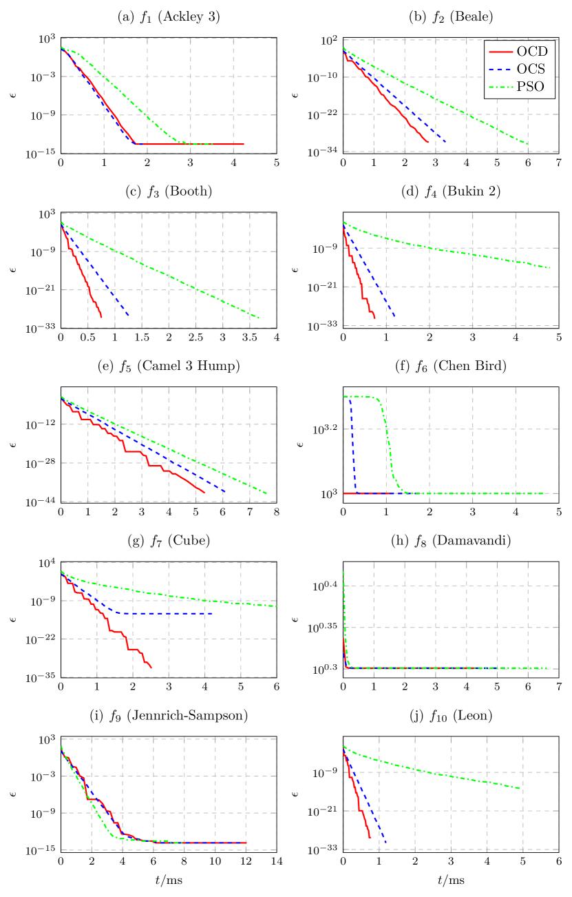
Figure 1: 2-dimensional functions

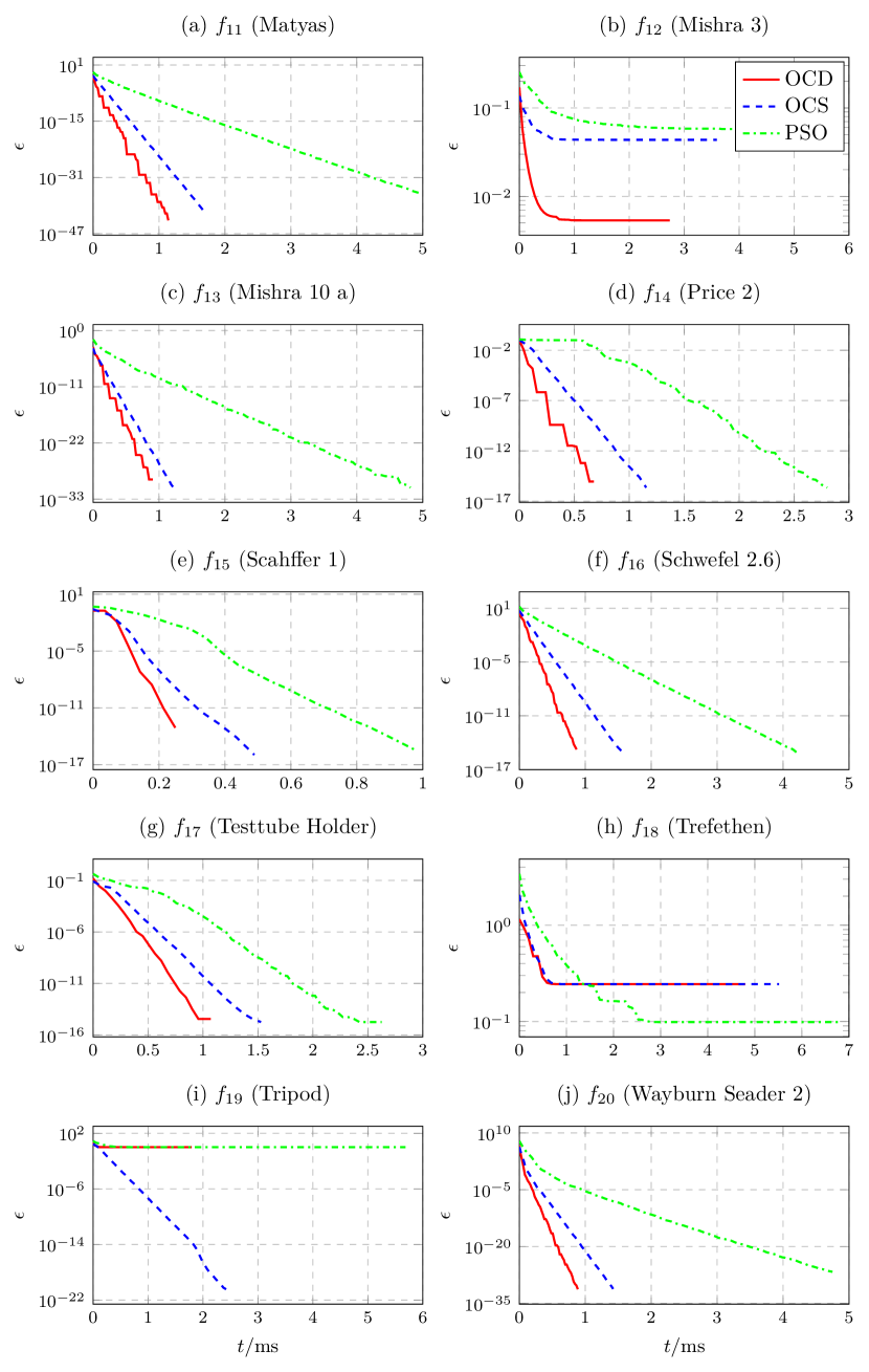
Figure 2: 2-dimensional functions

Table 1: Final error and computational time ($2$-dimensional cases)

		$\epsilon$	$t/s$		$\epsilon$	$t/s$
$f_{1}$	OCD	$2.8422\times 10^{-14}$	$0.0042$	$f_{6}$	$1000.0040$	$0.0011$
	OCS	$0$	$0.0040$		$1000.0040$	$0.0018$
	PSO	$0$	$0.0065$		$1000.0040$	$0.0047$
$f_{2}$	OCD	$0$	$0.0036$	$f_{7}$	$0$	$0.0032$
	OCS	$0$	$0.0044$		$3.9226\times 10^{-14}$	$0.0042$
	PSO	$0$	$0.0064$		$1.0660\times 10^{-11}$	$0.0061$
$f_{3}$	OCD	$0$	$0.0010$	$f_{8}$	$2$	$0.0043$
	OCS	$0$	$0.0017$		$2$	$0.0053$
	PSO	$0$	$0.0047$		$2$	$0.0066$
$f_{4}$	OCD	$0$	$0.0010$	$f_{9}$	$1.4211\times 10^{-14}$	$0.0120$
	OCS	$0$	$0.0016$		$1.4211\times 10^{-14}$	$0.0117$
	PSO	$9.0709\times 10^{-16}$	$0.0048$		$1.4211\times 10^{-14}$	$0.0080$
$f_{5}$	OCD	$4.0486\times 10^{-41}$	$0.0053$	$f_{10}$	$0$	$0.0011$
	OCS	$2.6048\times 10^{-41}$	$0.0062$		$0$	$0.0016$
	PSO	$2.5274\times 10^{-41}$	$0.0076$		$8.3655\times 10^{-15}$	$0.0050$

Table 2: Final error and computational time ($2$-dimensional cases)

		$\epsilon$	$t/s$		$\epsilon$	$t/s$
$f_{11}$	OCD	$6.2640\times 10^{-44}$	$0.0011$	$f_{16}$	$0$	$0.0011$
	OCS	$7.8040\times 10^{-42}$	$0.0017$		$0$	$0.0019$
	PSO	$4.1578\times 10^{-36}$	$0.0049$		$0$	$0.0049$
$f_{12}$	OCD	$0.0054$	$0.0027$	$f_{17}$	$0$	$0.0028$
	OCS	$0.0436$	$0.0036$		$0$	$0.0037$
	PSO	$0.0565$	$0.0052$		$0$	$0.0050$
$f_{13}$	OCD	$0$	$0.0014$	$f_{18}$	$0.2442$	$0.0048$
	OCS	$0$	$0.0018$		$0.2442$	$0.0055$
	PSO	$1.8527\times 10^{-31}$	$0.0048$		$0.0987$	$0.0068$
$f_{14}$	OCD	$0$	$0.0020$	$f_{19}$	$1$	$0.0018$
	OCS	$0$	$0.0030$		$3.5555\times 10^{-21}$	$0.0024$
	PSO	$0$	$0.0052$		$1$	$0.0057$
$f_{15}$	OCD	$0$	$0.0017$	$f_{20}$	$0$	$0.0010$
	OCS	$0$	$0.0027$		$0$	$0.0017$
	PSO	$0$	$0.0048$		$2.0474\times 10^{-27}$	$0.0047$

The evolution of the median error $\epsilon=f-f(\bm{x}^{\ast})$ with respect to the average computational time $t$ for each objective function is shown in Fig. 1 and 2. Moreover, the final error and computational time are collected in Tab. 1 and 2 for ease of comparison. From Fig. 1 and 2 we see that for most objective functions, the proposed OCD and OCS schemes converge to a global minimum faster than the PSO scheme and the OCD scheme is the best in terms of convergence rate. Moreover, from Tab. 1 and 2 we see that for most objective functions, the proposed OCD and OCS schemes consume less computational time than the PSO scheme even though they require more evaluations and have higher accuracy. From our perspective, this advantage stem from the simplicity of the proposed schemes. Specifically, they only need to update, in each iteration, the upper and lower bounds of a rectangular region by Eq. 3, which is computationally much simpler than the updating rules 2 of the PSO.

4.2 4-dimensional case

In the $4$-dimensional case, the proposed OCD and OCS schemes are also compared with the PSO scheme. For both the OCD and OCS schemes, the number of iterations is set to $200$ and the parameter $\lambda$ is set to $0.8$. The number of samples per iteration is $N^{D}=8^{4}=4096$ for the OCD scheme and $N=2000$ for the OCS scheme, which correspond to a total of $200\times 4096=819200$ and $200\times 2000=400000$ evaluations of each objective function, respectively. For the PSO scheme, the parameters $w=0.5$ and $c_{1}=c_{2}=1.5$. The number of iterations is set to $200$ and the number of particles is set to $1000$ which correspond to a total of $200\times 1000=200000$ evaluations of each objective function.

The evolution of the error $\epsilon$ with respect to the computational time $t$ is presented in Fig. 3. The final error and the computational time are collected in Tab. 3 for ease of comparison. In this case, we can draw a roughly the same conclusion as the $2$-dimensional case, so we are not going to repeat it here.

Figure 3: 4-dimensional functions

Table 3: Final error and computational time ($4$-dimensional cases)

		$\epsilon$	$t/s$		$\epsilon$	$t/s$
$f_{21}$	OCD	$0$	$0.1272$	$f_{26}$	$4.4867\times 10^{-18}$	$0.1566$
	OCS	$3.2712\times 10^{-8}$	$0.0945$		$1.9786\times 10^{-18}$	$0.1041$
	PSO	$1.7311\times 10^{-28}$	$0.1407$		$6.7831\times 10^{-17}$	$0.1238$
$f_{22}$	OCD	$0$	$0.0139$	$f_{27}$	$6.6267\times 10^{-5}$	$0.0866$
	OCS	$0$	$0.0236$		$4.3602\times 10^{-7}$	$0.0666$
	PSO	$1.9093\times 10^{-20}$	$0.0815$		$4.4452\times 10^{-8}$	$0.1052$
$f_{23}$	OCD	$0$	$0.0638$	$f_{28}$	$0$	$0.0271$
	OCS	$0$	$0.0587$		$0$	$0.0340$
	PSO	$0$	$0.0956$		$5.0524$	$0.0800$
$f_{24}$	OCD	$2444.2318$	$0.9708$	$f_{29}$	$0$	$0.0362$
	OCS	$2521.9434$	$0.6238$		$0$	$0.0442$
	PSO	$6.4308\times 10^{-24}$	$0.5506$		$0$	$0.0894$
$f_{25}$	OCD	$2.0377\times 10^{-11}$	$0.0222$	$f_{30}$	$1.7764\times 10^{-15}$	$0.0526$
	OCS	$2.0377\times 10^{-11}$	$0.0348$		$0$	$0.0441$
	PSO	$2.0377\times 10^{-11}$	$0.0882$		$0$	$0.0993$

4.3 30-dimensional case

In the $30$-dimensional case, only the results of the OCS and PSO schemes are compared, since the OCD scheme is not applicable. For the OCS scheme, the number of iterations is set to $2000$ and the parameter $\lambda$ is set to $0.98$. The number of samples per iteration is $N=1000$, which corresponds to a total of $2000\times 1000=2000000$ evaluations of each objective function. For the PSO scheme, the parameters $w=0.5$ and $c_{1}=c_{2}=1.5$. The number of iterations is set to $500$ and the number of particles is set to $2000$ which correspond to a total of $500\times 2000=1000000$ evaluations of each objective function.

The evolution of the error $\epsilon$ with respect to the computational time $t$ is presented in Fig. 4 and 5. The final error and the computational time are collected in Tab. 4 for ease of comparison. From Fig. 4 and 5, we see that in this case, both the OCS and PSO schemes can be easily trapped into a local minimum, especially when the objective function has lots of local minima. Moreover, compared to the PSO, it seems that the proposed OCS scheme tends to be trapped into a worse local minimum. From our point of view, the reason is that a swarm of particles is more flexibility than a single rectangular region. However, if a global minimum can be located, then the proposed OCS still converge faster than the PSO in most cases. In addition, it can be seen from Tab. 4 that the OCS is more efficient for functions that are easy to evaluate (which correspond to functions with lower computational time in the table). This is in sharp contrast to the Bayesian optimization which is more suitable for functions that are hard to evaluate.

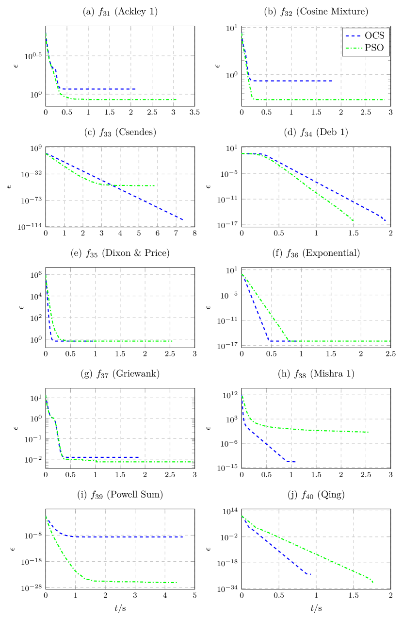
Figure 4: n-dimensional functions

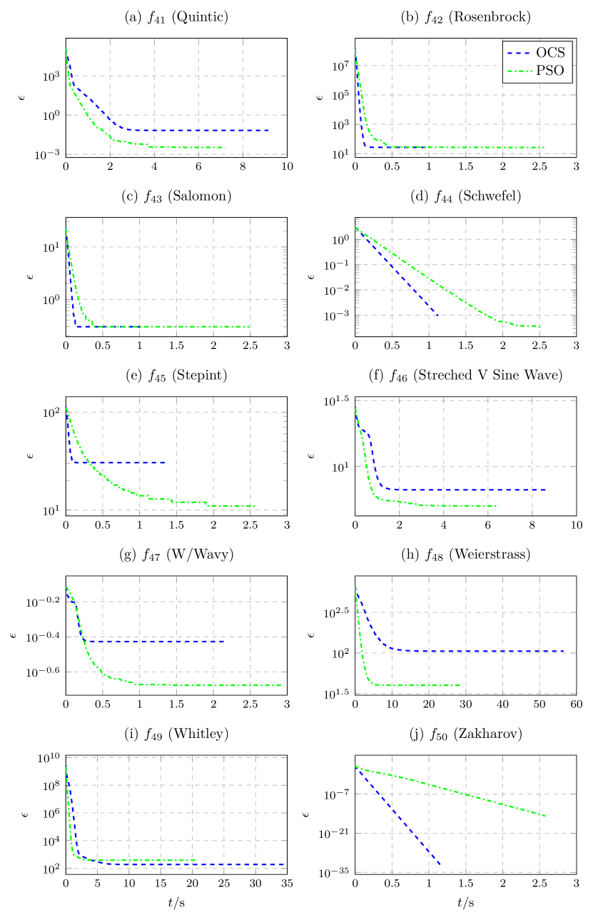
Figure 5: n-dimensional functions

Table 4: Final error and computational time ($30$-dimensional cases)

		$\epsilon$	$t/s$		$\epsilon$	$t/s$
$f_{31}$	OCS	$1.1672$	$2.1250$	$f_{41}$	$0.0670$	$9.1476$
	PSO	$0.8509$	$3.0647$		$0.0033$	$7.1850$
$f_{32}$	OCS	$0.7389$	$1.8674$	$f_{42}$	$26.7760$	$0.9567$
	PSO	$0.2956$	$2.8825$		$26.0295$	$2.5608$
$f_{33}$	OCS	$4.0252\times 10^{-105}$	$7.4280$	$f_{43}$	$0.2999$	$1.0038$
	PSO	$6.4725\times 10^{-51}$	$5.8337$		$0.2999$	$2.4848$
$f_{34}$	OCS	$0$	$3.7868$	$f_{44}$	$9.4634\times 10^{-4}$	$1.1233$
	PSO	$0$	$3.9395$		$3.4933\times 10^{-4}$	$2.5330$
$f_{35}$	OCS	$0.6667$	$0.9560$	$f_{45}$	$30.5000$	$1.3904$
	PSO	$0.6672$	$2.5456$		$11$	$2.5996$
$f_{36}$	OCS	$1.1102\times 10^{-16}$	$0.9779$	$f_{46}$	$6.6715$	$8.6658$
	PSO	$1.1102\times 10^{-16}$	$2.5115$		$5.0310$	$6.5056$
$f_{37}$	OCS	$0.0123$	$1.8930$	$f_{47}$	$0.3740$	$2.1925$
	PSO	$0.0074$	$2.9656$		$0.2107$	$2.9587$
$f_{38}$	OCS	$1.2390\times 10^{-13}$	$1.1133$	$f_{48}$	$105.5264$	$56.5051$
	PSO	$0.0137$	$2.5571$		$40.1300$	$28.4343$
$f_{39}$	OCS	$2.1256\times 10^{-09}$	$4.5957$	$f_{49}$	$190.5336$	$35.4969$
	PSO	$8.9848\times 10^{-27}$	$4.4360$		$392.3549$	$20.4798$
$f_{40}$	OCS	$8.9634\times 10^{-26}$	$0.9288$	$f_{50}$	$6.3418\times 10^{-33}$	$1.1509$
	PSO	$0$	$2.4371$		$1.5273\times 10^{-15}$	$2.5765$

5 Conclusions

In this paper, a new frame work for global optimization is proposed. Although it has a very simple form, it is effective for most of the benchmark functions. Compared to the PSO, the proposed frame work can generate new sample points at a lower computational cost. However, when the objective function is of high dimension and has lots of local minima, it usually requires more evaluations to avoid getting trapped into a local minimum since the utilization efficiency of samples is also lower. The reason is that in generating new sample points, only the information of the current best point is used. In this regard, it is more suitable for functions that are easy to evaluate which is in sharp contrast to the Bayesian optimization. On the other hand, if a global minimum can be located, then the proposed frame work usually converge faster than the PSO. From this point of view, the proposed frame work is more suitable for functions with a moderate dimension or a moderate number of local minima.

Future works should be focus on improving the utilization efficiency of sample points and preventing the algorithm from being trapped into a local minimum. From our perspective, a promising direction is to maintain multiple rectangular subregions in each iteration.

References

References

- [1] S. Boyd, L. Vandenberghe, Convex optimization, Cambridge university press, 2004.
- [2] V. Torczon, On the convergence of pattern search algorithms, SIAM Journal on optimization 7 (1) (1997) 1–25.
- [3] C. G. E. Boender, A. R. Kan, G. Timmer, L. Stougie, A stochastic method for global optimization, Mathematical programming 22 (1) (1982) 125–140.
- [4] R. H. Byrd, C. L. Dert, A. H. R. Kan, R. B. Schnabel, Concurrent stochastic methods for global optimization, Mathematical Programming 46 (1) (1990) 1–29.
- [5] M. Gaviano, D. Lera, A global minimization algorithm for lipschitz functions, optimization Letters 2 (1) (2008) 1–13.
- [6] C. Malherbe, N. Vayatis, Global optimization of lipschitz functions, in: International Conference on Machine Learning, PMLR, 2017, pp. 2314–2323.
- [7] I. P. Androulakis, C. D. Maranas, C. A. Floudas, bb: A global optimization method for general constrained nonconvex problems, Journal of Global Optimization 7 (4) (1995) 337–363.
- [8] C. S. Adjiman, S. Dallwig, C. A. Floudas, A. Neumaier, A global optimization method, bb, for general twice-differentiable constrained nlps—i. theoretical advances, Computers & Chemical Engineering 22 (9) (1998) 1137–1158.
- [9] C. S. Adjiman, I. P. Androulakis, C. A. Floudas, A global optimization method, bb, for general twice-differentiable constrained nlps—ii. implementation and computational results, Computers & chemical engineering 22 (9) (1998) 1159–1179.
- [10] T. G. Epperly, E. N. Pistikopoulos, A reduced space branch and bound algorithm for global optimization, Journal of Global Optimization 11 (3) (1997) 287–311.
- [11] D. R. Jones, M. Schonlau, W. J. Welch, Efficient global optimization of expensive black-box functions, Journal of Global optimization 13 (4) (1998) 455–492.
- [12] E. Solak, R. Murray-Smith, W. E. Leithead, D. J. Leith, C. E. Rasmussen, Derivative observations in gaussian process models of dynamic systems.
- [13] J. R. Gardner, M. J. Kusner, Z. E. Xu, K. Q. Weinberger, J. P. Cunningham, Bayesian optimization with inequality constraints., in: ICML, Vol. 2014, 2014, pp. 937–945.
- [14] C. K. Williams, C. E. Rasmussen, Gaussian processes for machine learning, Vol. 2, MIT press Cambridge, MA, 2006.
- [15] P. I. Frazier, A tutorial on bayesian optimization, arXiv preprint arXiv:1807.02811.
- [16] M. Mitchell, An introduction to genetic algorithms, MIT press, 1998.
- [17] D. E. Goldberg, J. H. Holland, Genetic algorithms and machine learning.
- [18] D. Greenhalgh, S. Marshall, Convergence criteria for genetic algorithms, SIAM Journal on Computing 30 (1) (2000) 269–282.
- [19] H.-P. P. Schwefel, Evolution and optimum seeking: the sixth generation, John Wiley & Sons, Inc., 1993.
- [20] H.-G. Beyer, H.-P. Schwefel, Evolution strategies–a comprehensive introduction, Natural computing 1 (1) (2002) 3–52.
- [21] Z. Li, X. Lin, Q. Zhang, H. Liu, Evolution strategies for continuous optimization: A survey of the state-of-the-art, Swarm and Evolutionary Computation 56 (2020) 100694.
- [22] K. Price, R. M. Storn, J. A. Lampinen, Differential evolution: a practical approach to global optimization, Springer Science & Business Media, 2006.
- [23] S. Das, P. N. Suganthan, Differential evolution: A survey of the state-of-the-art, IEEE transactions on evolutionary computation 15 (1) (2010) 4–31.
- [24] W. Deng, H. Liu, J. Xu, H. Zhao, Y. Song, An improved quantum-inspired differential evolution algorithm for deep belief network, IEEE Transactions on Instrumentation and Measurement 69 (10) (2020) 7319–7327.
- [25] D. Bratton, J. Kennedy, Defining a standard for particle swarm optimization, in: 2007 IEEE swarm intelligence symposium, IEEE, 2007, pp. 120–127.
- [26] J. Kennedy, R. Eberhart, Particle swarm optimization, in: Proceedings of ICNN’95-international conference on neural networks, Vol. 4, IEEE, 1995, pp. 1942–1948.
- [27] R. Poli, J. Kennedy, T. Blackwell, Particle swarm optimization, Swarm intelligence 1 (1) (2007) 33–57.
- [28] M. D. McKay, R. J. Beckman, W. J. Conover, A comparison of three methods for selecting values of input variables in the analysis of output from a computer code, Technometrics 42 (1) (2000) 55–61.
- [29] M. Jamil, X.-S. Yang, A literature survey of benchmark functions for global optimisation problems, International Journal of Mathematical Modelling and Numerical Optimisation 4 (2) (2013) 150–194.
-
[30]
A. R. Al-Roomi,
Unconstrained
Single-Objective Benchmark Functions Repository (2015).
URL https://www.al-roomi.org/benchmarks/unconstrained - [31] Y. Chen, Computer simulation of electron positron annihilation process, Stanford University, 2003.
- [32] M. Biggs, Minimization algorithms making use of non-quadratic properties of the objective function, IMA Journal of Applied Mathematics 8 (3) (1971) 315–327.
- [33] P. N. Suganthan, N. Hansen, J. J. Liang, K. Deb, Y.-P. Chen, A. Auger, S. Tiwari, Problem definitions and evaluation criteria for the cec 2005 special session on real-parameter optimization, KanGAL report 2005005 (2005) (2005) 2005.
- [34] T. Jumonji, G. Chakraborty, H. Mabuchi, M. Matsuhara, A novel distributed genetic algorithm implementation with variable number of islands, in: 2007 IEEE Congress on Evolutionary Computation, IEEE, 2007, pp. 4698–4705.