Syndrome decoding by quantum approximate optimization

Abstract

The syndrome decoding problem is known to be NP-hard. We use the quantum approximate optimization algorithm (QAOA) to solve the syndrome decoding problem with elegantly-designed generator- and check-based cost Hamiltonians for classical and quantum codes. Simulations of the level-4 check-based QAOA decoding of the [7,4,3] Hamming code, as well as the level-4 generator-based QAOA decoding of the [[5,1,3]] quantum code, demonstrate decoding performances that match the maximum likelihood decoding. In addition, we show that a combinatorial optimization problem with additional redundant clauses may be more suitable for QAOA, while the number of qubits remains the same. Furthermore, we show that the QAOA decoding of a quantum code is inherently degenerate. That is, degenerate errors of comparable weight will be returned by QAOA with comparable probability. This is supported by simulations of the generator-based QAOA decoding of the [[9,1,3]] Shor code.

I Introduction

Quantum computers provide extraordinary computation power by exploiting quantum effects. Farhi, Goldstone, and Gutmann proposed a class of heurisitic algorithms, the quantum approximate optimization algorithm (QAOA), which can find approximate solutions to combinatorial optimization problems that are computationally hard for classical computers [FGG14a, FGG14b]. A combinatorial optimization problem is embedded into a cost Hamiltonian so that the eigenstate with the largest eigenvalue is the optimal solution. Then the QAOA iterates between classical and quantum computers and outputs a distribution of the solutions, from which one can deduce an approximate solution. The approximate solution is closer to the optimal as the number of iterations (called levels) increases. Although the computation with a larger quantum circuit depth could be more powerful [CCL20, CM20], the QAOA with only one iteration (level-1 QAOA) may be able to demonstrate a quantum advantage [FH16]. Since the QAOA outputs approximate solutions, rather than exact ones, it does not require the hardware standard for universal fault-tolerant quantum computation and may be suitable for near-term quantum devices with tens or hundreds of qubits [MBB+18].

Consider the following syndrome decoding problem.

Definition 1.

[Syndrome decoding of a binary linear code] Given a (parity-check) matrix $H\in\{0,1\}^{r\times n}$, a binary (syndrome) vector ${\bm{z}}\in\{0,1\}^{r}$, and a nonnegative integer $w$, find a vector ${\bm{e}}\in\{0,1\}^{n}$ of Hamming weight no larger than $w$ such that ${{\bm{e}}}H^{T}={\bm{z}}$.

The associated decision problem of Def. 1 is known to be NP hard [BMVT78], even with preprocessing [BN90]. A generator matrix of a linear code is orthogonal to its parity-check matrix and the decoding problem can be formulated in terms of the generator matrix as well [MS77]. We will study the QAOA formulation of this decoding problem.

There is also a related channel decoding problem: find a vector in the rowspace of a generator matrix that is closest to a given vector. It has been studied by Bruck and Blaum [BB89] that an error-correcting code can be described by an energy function, with the peaks of the topography being the codewords. The decoding of a corrupted word is then equivalent to looking for the closest peak in the energy function. Previously, Matsumine, Koike-Akino, and Wang studied this channel decoding by QAOA [MKAW19]. (We emphasize that their cost Hamiltonian is basically the energy function defined by Bruck and Blaum [BB89].) The results in [MKAW19] suggested that the cost Hamiltonian defined by a low-density generator matrix (LDGM) is more suitable for the level-1 QAOA. A vector of high weight leads to an interaction between many qubits and thus a sparse matrix is desired.

On the other hand, linear codes defined by low-density parity-check (LDPC) matrices are capacity-approaching codes [Gal63]. Specifically, there exist good LDPC codes with row and column overlaps no larger than one [KLF01]. They have efficient decoders and are popular in applications. However, the generator matrix of an LDPC code is usually not sparse. Consequently, a parity-check based decoder is necessary.

In the quantum regime, binary quantum codes are like classical quaternary additive codes that are dual-containing [CRSS98]. We have a similar syndrome-based (bounded-distance) decoding problem that is also NP-hard [HG11, KL13_20]. (Unless the Steane or Knill syndrome extraction methods are used [Ste97L, Knill05, ZLB+20], a quantum decoding problem is in general syndrome-based.) Moreover, quantum codes allow degenerate errors so that different Pauli errors may have the same effects on the code space and they can be corrected by the same recovery operation. Therefore, the optimal decoding rule is to find the coset of degenerate errors with the largest probability condition on a given syndrome, which induces a $\#P$ hard problem [IP15]. This degeneracy is not considered by a conventional belief propagation decoder [MMM04, KL20]; however, degeneracy can still be exploited in belief propagation so that a decoder may output degenerate errors [KL21].

In this paper we will define two cost Hamiltonians according to the generator or parity-check matrices for the QAOA decoding of a classical or quantum code. The generator-based Hamiltonian is similar to that in [MKAW19], following the idea in [BB89]. The check-based Hamiltonian is involved with two terms: one for parity-check satisfaction and the other for error weight. A low-weight error that matches all the parity checks is preferred. We introduce two parameters to adjust the proportion of these two terms. In both Hamiltonians, the formulations are more complicated in the quantum case due to the notion of generalized Hamming weight for Pauli errors.

We remark that the QAOA decoding of a quantum code is degenerate. In [LP19], Liu and Poulin engineered an objective function for a neural network to have a few low-weight degenerate errors so that their neural network decoder is able to return degenerate errors [LP19]. In contrast, the QAOA decoding starts with an equally-weighted superposition of all solutions. Because of the designed cost Hamiltonian, a degenerate error of comparable weight will appear in the output distribution of the QAOA with comparable probability.

Finally, we simulate the level-$p$ QAOA decoding of the classical $[7,4,3]$ Hamming code, the unique $[[5,1,3]]$ quantum code, and the $[[9,1,3]]$ Shor code [Shor95] for $p\leq 4$. We show that the level-$4$ check-based QAOA decoding of the $[7,4,3]$ Hamming code matches the optimal maximum-likelihood decoding. The parity-check matrix of the $[7,4,3]$ Hamming code is pretty dense, so we may expect that the check-based QAOA decoding performs well for larger codes with sparse parity-check matrices. For the quantum case, the generator matrix of the $[[5,1,3]]$ code is dense. The level-$4$ generator-based QAOA decoding of the $[[5,1,3]]$ code, based on the generalized weight, matches the optimal maximum-likelihood decoding.

Simulations of the level-$p$ generator-based QAOA decoding of the $[[9,1,3]]$ Shor code are conducted since the generator-based cost Hamiltonian requires fewer qubits than the check-based one. However, a complete decoding performance curve is still difficult to simulate for $p>2$. Instead, we compare the output distribution of the QAOA to the real conditional distribution according to the channel statistics. We show that the QAOA output distribution is close to the real distribution for certain error syndromes in terms of the Jensen–Shannon divergence [ES03]. Moreover, we show that an $Z$ error on anyone of the first three qubits is returned with close probabilities by the QAOA as they are degenerate errors of the same weight, which justifies that the QAOA decoding of a quantum code is degenerate.

A level-$p$ QAOA has $2p$ parameters ${\bm{\gamma}}$ and ${\bm{\beta}}\in[0,\pi]^{p}$ that need to be determined by a classical computer, and derivative-free optimization methods are preferred [SSL19]. In our simulations, the python software SciPy [Vir+20] is used, which supports derivative-free methods, such as the Nelder-Mead (NM) method [NM65] and constrained optimization by linear approximation (COBYLA) [Pow78, Pow94]. The optimization problem of determining optimal angles ${\bm{\gamma}}$ and ${\bm{\beta}}$ is not convex, so an optimization tool may not return angles ${\bm{\gamma}}$ and ${\bm{\beta}}$ that are actually good. Thus the multistart method is used so that multiple NM or COBYLA are executed with different starting points $(\bm{\gamma},\bm{\beta})$ (see [SSL19] for more details). Heuristic optimization by basin-hopping is also employed [WD97].

We remark that it is possible to define an equivalent problem with additional redundant clauses so that its Hamiltonian is easier for optimization by QAOA, while the complexity remains the same. This will be shown by the check-based decoding of the $[7,4,3]$ code, which is a cyclic code with an $n\times n$ parity-check matrix with rows cyclicly generated. So every bit is equally protected. Note that the same strategy has been used to improve the BP decoding performance (e.g., see [KL21b, Appendix B]) but the complexity of the classical algorithm will increase.

On the other hand, the problem density of a QAOA is defined as the number of clauses divided by the number of qubits, $q/m$, [APMB20]. The relations between the problem density and the performance of a QAOA were studied and it is known that if $q/m>1$, then QAOA may have reachability deficits [APMB20]. The problem density is higher with additional clauses for decoding. However, for check-based classical decoding and generator-based quantum decoding, we have $q/m\leq 1$ and thus we do not encounter such problems in all our simulations.

This paper is organized as follows. We review the basics of the QAOA in the next section. In Sections III and IV, we define the generator- and check-based cost Hamiltonians for classical and quantum codes, respectively. Simulations of the $[7,4,3]$ Hamming code, the $[[5,1,3]]$ quantum code, and the $[[9,1,3]]$ Shor code are provided in Sec. V. Then we conclude in Section LABEL:sec:con.

II Quantum approximate optimization algorithm

We consider quantum information in qubits with the computational basis $\{|0\rangle,|1\rangle\}$. The Pauli matrices in the computational basis are ${\hat{I}}=\left[\begin{matrix}1&0\\ 0&1\end{matrix}\right],~{}\hat{X}=\left[\begin{matrix}0&1\\ 1&0\end{matrix}\right],~{}\hat{Y}=\left[\begin{matrix}0&-i\\ i&0\end{matrix}\right],~{}{{\hat{Z}}=\left[\begin{matrix}1&0\\ 0&-1\end{matrix}\right].}$ The $m$-fold Pauli group $\mathcal{G}_{m}$ is $\mathcal{G}_{m}=\left\{i^{c}M_{1}\otimes\cdots\otimes M_{m}:\,c\in\{0,1,2,3\},\,M_{j}\in\{\hat{I},\hat{X},\hat{Y},\hat{Z}\}\right\}.$ Let ${\hat{X}}_{j}$ (${\hat{Z}_{j}}$) denote the quantum operator with ${\hat{X}}$ (${\hat{Z}}$) on the $j$th qubit and identity on the others. Let $I$ denote the identity operator with appropriate dimension. Sometimes we may omit the tensor product symbol in an $m$-fold Pauli operator. For example, $\hat{X}\otimes\hat{Y}\otimes\hat{Z}\otimes\hat{I}\otimes\hat{I}=\hat{X}\hat{Y}\hat{Z}\hat{I}\hat{I}=\hat{X}_{1}\hat{Y}_{2}\hat{Z}_{3}$.

Herein a combinatorial optimization problem with variable ${{\bm{x}}}=(x_{1},x_{2},\dots,x_{m})\in\{0,1\}^{m}$ is as follows:

$$\text{maximum }C({{\bm{x}}})=\sum_{j=1}^{q}C_{j}({{\bm{x}}}).$$ (1)

The objective function $C:\{0,1\}^{m}\rightarrow\mathbb{R}$ is defined by $q$ clause functions $C_{j}:\{0,1\}^{m}\rightarrow\{+1,-1\}$, where

$$C_{j}({{\bm{x}}})=\begin{cases}+1,&\mbox{ if ${{\bm{x}}}$ satisfies clause $j$};\\ -1,&\mbox{ otherwise.}\end{cases}$$ (2)

This combinatorial optimization problem can be handled by an QAOA with $m$ qubits in Algorithm 1. A cost Hamiltonian operator corresponding to the objective function $C({\bm{x}})$ is defined by

$$\hat{C}=\sum_{j=1}^{q}{\hat{C}}_{j},$$ (3)

where ${\hat{C}}_{j}$ is a Hermitian operator corresponding to clause $C_{j}$ and is defined as

$$\hat{C}_{j}=\sum_{{{\bm{e}}}\in\{0,1\}^{m}}C_{j}({\bm{e}})|{\bm{e}}\rangle\langle{\bm{e}}|,$$ (4)

with respect to the computational basis vector $|{\bm{e}}\rangle$. We remark that our choice of cost Hamiltonian has eigenvalues $\{-q,-q+2,\dots,q-2,q\}$ because of Eq. (2), which is different from that in [FGG14a].

Consider a Hermitian operator $\hat{B}=\sum_{j=1}^{m}\hat{X}_{j}.$ The eigenvector corresponding to the largest eigenvalue of $\hat{B}$ is $|\psi_{0}\rangle=|+\rangle^{\otimes m}=\left(\frac{|0\rangle+|1\rangle}{\sqrt{2}}\right)^{m}$ and it will be the initial state to the QAOA.

Define unitary operators

$$U(\hat{C},\gamma)= e^{-i\gamma\hat{C}}=\prod_{j=1}^{q}e^{-i\gamma\hat{C}_{j}},$$ (5)

and

$$U(\hat{B},\beta)= e^{-i\beta\hat{B}}=\prod_{j=1}^{m}e^{-i\beta\hat{X}_{j}},$$ (6)

where $\gamma,\beta\in[0,\pi]$. Note that the energy gap between any two adjacent energy levels is two in $\hat{C}$ or $\hat{B}$, so both the periods of $\gamma$ and $\beta$ are $\pi$.

For any integer $p\geq 1$, a $p$-level QAOA uses quantum alternating operator ansatz circuits of depth $p$ to generate an angle-dependent quantum state

$$|\psi_{\bm{\gamma},\bm{\beta}}\rangle=U(\hat{B},\beta_{p})U(\hat{C},\gamma_{p})\cdots U(\hat{B},\beta_{1})U(\hat{C},\gamma_{1})|\psi_{0}\rangle.$$ (7)

with $2p$ angles $\bm{\gamma}=(\gamma_{1},\dots,\gamma_{p})\in[0,\pi]^{p}$ and $\bm{\beta}=(\beta_{1},\dots,\beta_{p})\in[0,\pi]^{p}$. Then the expectation of the objective $\hat{C}$ on this state $|\psi_{\bm{\gamma},\bm{\beta}}\rangle$ is

$$F_{p}(\bm{\gamma},\bm{\beta})=\langle\psi_{\bm{\gamma},\bm{\beta}}|\hat{C}|\psi_{\bm{\gamma},\bm{\beta}}\rangle.$$ (8)

Let $M_{p}$ be the maximum of $F_{p}(\bm{\gamma},\bm{\beta})$ over the angles $\gamma_{1},\dots,\gamma_{p},\beta_{1},\dots,\beta_{p}$. As $p$ increases, $M_{p}$ is closer to the optimal value $\max_{\bm{x}}C(\bm{x})$. The procedure of a $p$-level QAOA is given in Algorithm 1.

Input : A cost Hamiltonian $\hat{C}$. The number of qubits $m$. An iteration number $T$.

Output: A distribution over $\{0,1\}^{m}$.

1. (Classical computer) Determine $2p$ parameters ${\bm{\gamma}}=\{\gamma_{1},\dots,\gamma_{p}\}\in[0,\pi]^{p}$ and ${\bm{\beta}}=\{\beta_{1},\dots,\beta_{p}\}\in[0,\pi]^{p}$.

2. (Quantum computer) Construct the state $|\psi_{{\bm{\gamma},\bm{\beta}}}\rangle$ in Eq. (7) with input $\hat{C}$.

3. (Quantum computer) Measure $|\psi_{{\bm{\gamma},\bm{\beta}}}\rangle$ in the computational basis and obtain outcome ${\bm{x}}\in\{0,1\}^{m}$.

4. Repeat steps 2) to 3) $T$ times and return the distribution of the measurement outcomes $\{{\bm{x}}\}$.

Algorithm 1 $p$-level QAOA with input $(\hat{C},m,T)$.

Finding the optimal angle sets $\{\gamma_{1},\dots,\gamma_{p}\}$ and $\{\beta_{1},\dots,\beta_{p}\}$ is a main obstacle for QAOA. One may use a fine grid method, which takes time ${O(\kappa^{2p})}$, where ${\kappa}$ is the number of possible values for each angle. Some optimization methods can also be applied and this will be discussed more in Sec. V.

III Syndrome decoding of classical linear codes

The goal of a classical decoding problem is to find the most possible error, or equivalently, finding the closet codeword to a received vector. Herein we propose syndrome decoders by QAOA for classical codes based on their generator or parity-check matrices. These results will be extended for quantum codes in the next section.

An $[n,k]$ classical linear code is the row space of a $k\times n$ generator matrix $G$ and its vectors are called codewords. It can also be defined as the null space of an $r\times n$ parity-check matrix ${H}$ of rank $(n-k)$. If a received vector ${\bm{y}}\in\{0,1\}^{n}$ is such that ${\bm{y}}H^{T}\neq\bm{0}$, then ${\bm{y}}$ is not a codeword. Thus the vector ${\bm{y}}H^{T}$ is called the error syndrome of ${\bm{y}}$ for any ${\bm{y}}\in\{0,1\}^{n}$. Given a syndrome vector ${\bm{s}}\in\{0,1\}^{r}$, the minimum weight decoding rule is to find

$$\operatorname*{arg\,min}_{\begin{subarray}{c}{\bm{e}}\in\{0,1\}^{n}\text{ s.t. }{\bm{e}}H^{T}={\bm{s}}\end{subarray}}\text{wt}\left({\bm{e}}\right),$$ (9)

where the (Hamming) weight of a vector ${\bm{y}}\in\{0,1\}^{n}$, denoted $\text{wt}\left({\bm{y}}\right)$, is the number of its nonzero entries. The Hamming distance between two vectors ${\bm{x}},{\bm{y}}\in\{0,1\}^{n}$ is $d_{H}({\bm{x}},{\bm{y}})=\text{wt}\left({\bm{x}}-{\bm{y}}\right)$.

III.1 Generator-based decoding

Suppose that ${\bm{z}}=(z_{1},\dots,z_{n})\in\{0,1\}^{n}$ satisfies that ${\bm{z}}H^{T}={\bm{s}}$. Such ${\bm{z}}$ can be efficiently found. Then an error vector ${\bm{e}}$ with ${\bm{e}}H^{T}={\bm{s}}$ can be written as ${\bm{e}}={\bm{u}}G+{\bm{z}}$ for some ${\bm{u}}\in\{0,1\}^{k}$. Consequently, Eq. (9) is equivalent to

$$\operatorname*{arg\,min}_{\begin{subarray}{c}{\bm{u}}\in\{0,1\}^{k}\end{subarray}}\text{wt}\left({\bm{u}}G+{\bm{z}}\right)\,=\, \operatorname*{arg\,min}_{\begin{subarray}{c}{\bm{u}}\in\{0,1\}^{k}\end{subarray}}d_{H}({\bm{u}}G+{\bm{z}},0)\,=\,\operatorname*{arg\,min}_{\begin{subarray}{c}{\bm{u}}\in\{0,1\}^{k}\end{subarray}}d_{H}({\bm{u}}G,{\bm{z}})\,=\,\operatorname*{arg\,max}_{\begin{subarray}{c}{\bm{u}}\in\{0,1\}^{k}\end{subarray}}\sum_{j=1}^{n}(1-2z_{j})(1-2[{\bm{u}}G]_{j}),$$ (10)

where $[{\bm{u}}G]_{j}$ denotes the $j$-th entry of ${\bm{u}}G$ and a mapping $\{0,1\}\mapsto\{+1,-1\}$ is used in the last equality.

The number of candidates ${\bm{u}}$ is $2^{k}$, and it would be impractical to test them in sequence by brute force when $k$ is large. Naturally, one would like to solve the maximization problem corresponding to Eq. (10) in an equivalent energy maximization problem. We define a corresponding cost Hamiltonian to solve Eq. (10) by QAOA using $k$ qubits [MKAW19]:

$$\hat{C}=\sum_{j=1}^{n}(1-2z_{j})\prod_{\ell=1}^{k}\hat{Z}_{\ell}^{[G]_{\ell,j}},$$ (11)

where $[G]_{\ell,j}$ is the $(\ell,j)$-th entry of $G$. Note that $\hat{Z}_{\ell}^{0}=I$ and $\hat{Z}_{\ell}^{1}=\hat{Z}_{\ell}$. One can verify that for ${\bm{u}}\in\{0,1\}^{k}$,

$$\left(\prod_{\ell=1}^{k}\hat{Z}_{\ell}^{[G]_{\ell,j}}\right)|{\bm{u}}\rangle=(1-2[{\bm{u}}G]_{j})|{\bm{u}}\rangle.$$ (12)

Hence finding an eigenvector of the cost Hamiltonian $\hat{C}$ defined in Eq. (11) with the largest eigenvalue is equivalent to Eq. (10). A generator-based syndrome decoding of a classical linear code by QAOA is summarized in Algorithm 2.

Input :  An $r\times n$ parity-check matrix $H$ and a syndrome ${\bm{s}}\in\{0,1\}^{r}$. Iteration number $T$.

Output: An error $\tilde{{\bm{e}}}\in\{0,1\}^{n}$ such that $\tilde{{\bm{e}}}H^{T}={\bm{s}}$.

1. Find a $k\times n$ generator matrix $G$ with respect to $H$ and a vector ${\bm{z}}\in\{0,1\}^{n}$ such that ${\bm{z}}H^{T}={\bm{s}}$. Let $\hat{C}$ be defined as in Eq. (11) using $G$ and ${\bm{z}}$.

2. Run Algorithm 1 with input ($\hat{C}$, $k$, $T$).

3. Get an estimate $\tilde{{\bm{u}}}$ from the output distribution by Algorithm 1 and return $\tilde{{\bm{e}}}=\tilde{{\bm{u}}}G+{\bm{z}}$.

Algorithm 2 Generator-based syndrome decoding of a classical code by QAOA.

Example 1.

Consider the $[7,4]$ Hamming code with generator and parity-check matrices

$$G=\begin{bmatrix}1&0&0&0&1&1&0\\ 0&1&0&0&1&0&1\\ 0&0&1&0&0&1&1\\ 0&0&0&1&1&1&1\end{bmatrix},~{}H=\begin{bmatrix}1&1&0&1&1&0&0\\ 1&0&1&1&0&1&0\\ 0&1&1&1&0&0&1\\ \end{bmatrix}.$$ (13)

Assume that the error syndrome is $(0,1,0)$. We find that the vector $(0,0,0,0,0,1,0)$ is of syndrome $(0,1,0)$. Thus the cost Hamiltonian is

$$\hat{C}={\hat{Z}_{1}+\hat{Z}_{2}+\hat{Z}_{3}+\hat{Z}_{4}+\hat{Z}_{1}\hat{Z}_{2}\hat{Z}_{4}-\hat{Z}_{1}\hat{Z}_{3}\hat{Z}_{4}+\hat{Z}_{2}\hat{Z}_{3}\hat{Z}_{4}}.$$

III.2 Check-based decoding

We may also define an energy Hamiltonian directly based on the parity-check matrix $H$. In [BB89], an energy topology is defined such that the errors corresponding to the given syndrome ${\bm{s}}$ are the points in the topology with the lowest energy. However, the weight of an error is not reflected in the energy topology so a modification is necessary.

We define the following check-based cost Hamiltonian for QAOA with $n$ qubits according to syndrome ${\bm{s}}=(s_{1}s_{2}\dots s_{r})\in\{0,1\}^{r}$:

$$\hat{C}={\eta}\sum_{j=1}^{r}(1-2s_{j})\prod_{\ell=1}^{n}{\hat{Z}_{\ell}^{[H]_{j,\ell}}}+{\alpha}\sum_{j=1}^{n}{\hat{Z}_{j}},$$ (14)

where the first term characterizes the parity-check satisfaction similarly to Eq. (11) and the second term is a penalty function for error weights. Note that $\alpha$ and $\eta$ are positive integers so that the values of $\gamma$’s remain in $[0,\pi]$.

Since $\hat{Z}=|0\rangle\langle 0|-|1\rangle\langle 1|$, every computational basis state is an eigenstate of $\sum_{j=1}^{n}{\hat{Z}_{j}}$ and a basis vector of lower weight would have a higher energy. This Hamiltonian is similar to the energy topology for belief propagation decoding of quantum codes defined in [KL21].

Example 2.

Consider the $[7,4]$ Hamming code again and assume the error syndrome $(0,1,0)$. Then the cost Hamiltonian is

$$\hat{C}= {\eta}\left(\hat{Z}_{1}\hat{Z}_{2}\hat{Z}_{4}\hat{Z}_{5}-\hat{Z}_{1}\hat{Z}_{3}\hat{Z}_{4}\hat{Z}_{6}+\hat{Z}_{2}\hat{Z}_{3}\hat{Z}_{4}\hat{Z}_{7}\right)+{\alpha}\sum_{i=1}^{7}\hat{Z}_{i}.$$

A check-based syndrome decoding of a classical code by QAOA is summarized in Algorithm 3.

Input :  An ${r}\times n$ parity-check matrix $H$ and a syndrome ${\bm{s}}\in\{0,1\}^{r}$. Iteration number $T$. Integers $\alpha,\eta>0$.

Output: An error $\tilde{{\bm{e}}}\in\{0,1\}^{n}$ such that $\tilde{{\bm{e}}}H^{T}={\bm{s}}$.

1. Let $\hat{C}$ be defined as in Eq. (14).

2. Run Algorithm 1 with input ($\hat{C}$, $n$, $T$).

3. Estimate $\tilde{{\bm{e}}}$ from the output distribution by Algorithm 1 and return $\tilde{{\bm{e}}}$.

Algorithm 3 Check-based syndrome decoding of a classical code by QAOA.

The measurement outcomes in QAOA are error candidates and a decision remains to be made upon receiving the distribution. A potential method is to first remove the vectors that do not match the syndrome and then choose the remaining vector with the lowest weight.

IV Syndrome decoding of quantum stabilizer codes

Suppose that $\mathcal{S}$ is an abelian subgroup of $\mathcal{G}_{n}$ such that $-{I}\notin\mathcal{S}$ and let $V$ be a $2^{n}$-dimensional complex inner product space with a standard basis $\{|{\bm{e}}\rangle:{\bm{e}}\in\{0,1\}^{n}\}.$ Define $\mathcal{C(S)}$ by

$$\mathcal{C(S)}\equiv\{|{\bm{v}}\rangle\in V:g|{\bm{v}}\rangle=|{\bm{v}}\rangle\ \forall\,g\in\mathcal{S}\}.$$

Suppose that $\mathcal{S}=\langle g_{1},\dots,g_{n-k}\rangle$ has $n-k$ independent generators. Then $\mathcal{C(S)}$ is a $2^{k}$-dimensional complex vector subspace of $V$ and is called an $[[n,k]]$ stabilizer code.

The discretization theorem says that if a set of error operators can be corrected by a quantum code, any linear combination of these error operators can also be corrected [NC00]. Thus we consider quantum errors that are tensor product of Pauli matrices.

Any two Pauli operators either commute or anticommute with each other. A Pauli error $E\in\mathcal{G}_{n}$ can be detected if it anticommutes with some stabilizers. So the error syndrome of $E$ with respect to a set $\{f_{1},\dots,f_{r}\}\subset\mathcal{S}$ that generate $\mathcal{S}$ is defined as ${\bm{s}}(E)=(s_{f_{1}}(E),\dots,s_{f_{r}}(E))$, where

$$s_{g}(E)=\begin{cases}0,&\text{if $gE=Eg$};\\ 1,&\text{if $gE=-Eg$}.\end{cases}$$ (15)

A Pauli operator $g\in\mathcal{G}_{n}$ can also be represented as $g=i^{c}\prod_{j=1}^{n}\hat{X}_{j}^{u_{j}}\hat{Z}_{j}^{v_{j}}$, where $u_{j},v_{j}\in\{0,1\}$. Define a homomorphism $\varphi:\mathcal{G}_{n}\mapsto\mathbb{Z}_{2}^{2n}$ on $g$ by $\varphi(g)=(u_{i},\dots,u_{n}|v_{1},\dots,v_{n})$. When the phase of a Pauli operator is irrelevant, it suffices to discuss its corresponding binary $2n$-tuple. Thus a check matrix corresponding to $\{f_{1},\dots,f_{r}\}$ is defined as

$${H}_{\mathcal{S}}\equiv\left[\begin{matrix}\varphi(f_{1})\\ \varphi(f_{2})\\ \vdots\\ \varphi(f_{r})\\ \end{matrix}\right],$$ (16)

which is an $r\times 2n$ binary matrix. Consequently, the error syndrome of a Pauli operator $E\in\mathcal{G}_{n}$ is

$${\bm{s}}(E)=\varphi(E)\Lambda{H}_{\mathcal{S}}^{T},$$ (17)

where $\Lambda=\begin{bmatrix}O_{n\times n}&{I}_{n\times n}\\ {I}_{n\times n}&O_{n\times n}\end{bmatrix}$, $I_{n\times n}$ is the $n\times n$ identity matrix, and $O_{n\times n}$ is an $n\times n$ all-zero matrix. Therefore, one can equivalently consider a binary code of length $2n$. However, the notion of weight is different; the weight of a Pauli operator $E$ is the generalized weight $\text{gw}\left(\varphi(E)\right)$ of the binary $2n$-tuple $\varphi(E)$, defined by

$$\text{gw}\left({\bm{v}}\right)\equiv\left|\{j\in\{1,\dots,n\}:v_{j}=1\mbox{ or }v_{n+j}=1\}\right|$$ (18)

for ${\bm{v}}=(v_{1},v_{2},\dots,v_{2n})\in\{0,1\}^{2n}$. When $n=1$, we have $\text{gw}\left((0,0)\right)=0$ and $\text{gw}\left((0,1)\right)=\text{gw}\left((1,0)\right)=\text{gw}\left((1,1)\right)=1$.

The normalizer group of $\mathcal{S}$ is

$$N(\mathcal{S})=\{g\in\mathcal{G}_{n}:gh=hg,\,\text{ for all }h\in\mathcal{S}\}.$$

One can find $g_{n-k+1},\dots,g_{n},$ $h_{n-k+1},\dots,h_{n}\in\mathcal{G}_{n}$ such that $N(\mathcal{S})$ is generated by $\{g_{1},\dots,g_{n},h_{n-k+1},\dots,h_{n}\}$ up to phases [CG97, NC00]. For $E\in\mathcal{G}_{n}$, one readily understand that $gE$ and $E$ have the same error syndrome for any $g\in N(\mathcal{S})$. Thus, there are $2^{n+k}$ errors, up to phases, with the same syndrome. Moreover, for $g\in\mathcal{S}$, $gE$ and $E$ have the same effects on the codespace and thus they are called degenerate errors of each other. The minimum distance of a quantum code is $d=\min\{\text{gw}\left(\varphi(g)\right):\,g\in N(\mathcal{S}),~{}g\notin\{\pm 1,\pm i\}\times\mathcal{S}\}.$ An $[[n,k,d]]$ quantum code is called a degenerate code if there exists nonidentity $g\in\mathcal{S}$ with $\text{gw}\left(\varphi(g)\right)<d$.

IV.1 Generator-based decoding

We will similarly devise a generator-based syndrome decoding of a quantum stabilizer code by QAOA. This is done by considering the dual of the binary code of length $2n$ defined by the check matrix Eq. (16) of an $n$-qubit quantum code.

Suppose that $N(\mathcal{S})$ is generated by $\{g_{1},\dots,g_{n},h_{n-k+1},\dots,h_{n}\}$ up to phases. Consider the matrix

$$G_{\mathcal{S}}=\left[\begin{smallmatrix}\varphi(g_{1})\\ \vdots\\ \varphi(g_{n})\\ \varphi(h_{n-k+1})\\ \vdots\\ \varphi(h_{n})\\ \end{smallmatrix}\right],$$ (19)

which satisfies $G_{\mathcal{S}}\Lambda H_{\mathcal{S}}^{T}=O$. Such $G_{\mathcal{S}}$ can be efficiently found, for example, by an encoding algorithm of the stabilizer code [CG97, NC00, KL19]. Given a syndrome ${\bm{s}}=(s_{1},\dots,s_{r})\in\{0,1\}^{r}$, one can efficiently find ${\bm{z}}=(z_{1},\dots,z_{2n})\in\{0,1\}^{2n}$ such that ${\bm{z}}\Lambda H_{\mathcal{S}}^{T}={\bm{s}}.$ Consequently a potential error is of the form

$${\bm{z}}+{\bm{u}}G_{\mathcal{S}}$$

for ${\bm{u}}\in\{0,1\}^{n+k}$. We can similarly define a cost Hamiltonian as in Sec. III.1. However, the notion of weight is different and we have to design a Hamiltonian regarding to the generalized weight. We define a generalized distance $d_{\text{gw}}({\bm{a}},{\bm{b}})=\text{gw}\left({\bm{a}}-{\bm{b}}\right)$ for ${\bm{a}},{\bm{b}}\in\{0,1\}^{2n}$. Then the minimum weight decision rule is

$$\operatorname*{arg\,min}_{\begin{subarray}{c}{\bm{u}}\in\{0,1\}^{n+k}\end{subarray}}\text{gw}\left({\bm{u}}G_{\mathcal{S}}+{\bm{z}}\right)= \operatorname*{arg\,min}_{\begin{subarray}{c}{\bm{u}}\in\{0,1\}^{n+k}\end{subarray}}d_{\text{gw}}({\bm{u}}G_{\mathcal{S}},{\bm{z}})=\operatorname*{arg\,min}_{\begin{subarray}{c}{\bm{u}}\in\{0,1\}^{n+k}\end{subarray}}\sum_{j=1}^{n}d_{\text{gw}}(([{\bm{u}}G_{\mathcal{S}}]_{j},[{\bm{u}}G_{\mathcal{S}}]_{n+j}),(z_{j},z_{n+j}))$$

$$= \operatorname*{arg\,max}_{\begin{subarray}{c}{\bm{u}}\in\{0,1\}^{n+k}\end{subarray}}\sum_{j=1}^{n}(-1)^{d_{\text{gw}}(([{\bm{u}}G_{\mathcal{S}}]_{j},[{\bm{u}}G_{\mathcal{S}}]_{n+j}),(z_{j},z_{n+j}))},$$ (20)

where a mapping $\{0,1\}\mapsto\{+1,-1\}$ is used in the last equality. For $a_{1},a_{2},b_{1},b_{2}\in\{0,1\}$, $d_{\text{gw}}\left((a_{1},a_{2}),(b_{1},b_{2})\right)=1$ if $a_{j}\neq b_{j}$ for some $j\in\{1,2\}$, and $d_{\text{gw}}\left((a_{1},a_{2}),(b_{1},b_{2})\right)=0$, otherwise. One can verify that

$$(-1)^{d_{\text{gw}}\left((a_{1},a_{2}),(b_{1},b_{2})\right)}=\frac{1}{2}\left((-1)^{a_{1}+b_{1}}+(-1)^{a_{2}+b_{2}}+(-1)^{a_{1}+b_{1}+a_{2}+b_{2}}-1\right).$$ (21)

Thus Eq. (20) can be rewritten as

$$\operatorname*{arg\,max}_{\begin{subarray}{c}{\bm{u}}\in\{0,1\}^{n+k}\end{subarray}} \frac{1}{2}\sum_{j=1}^{n}\left((-1)^{z_{j}}(-1)^{[{\bm{u}}G_{\mathcal{S}}]_{j}}+(-1)^{z_{n+j}}(-1)^{[{\bm{u}}G_{\mathcal{S}}]_{n+j}}\right.\left.+(-1)^{z_{j}}(-1)^{z_{n+j}}(-1)^{[{\bm{u}}G_{\mathcal{S}}]_{j}}(-1)^{[{\bm{u}}G_{\mathcal{S}}]_{n+j}}-1\right).$$ (22)

Therefore, we define a generator-based cost Hamiltonian for a quantum stabilizer code with syndrome ${\bm{s}}$ as

$$\hat{C}=\frac{1}{2}\sum_{j=1}^{n}\left((1-2z_{j})\prod_{\ell=1}^{n+k}\hat{Z}_{\ell}^{[G_{\mathcal{S}}]_{\ell,j}}+(1-2z_{n+j})\prod_{\ell=1}^{n+k}\hat{Z}_{\ell}^{[G_{\mathcal{S}}]_{\ell,n+j}}\right.+\left.(1-2z_{j})(1-2z_{n+j})\prod_{\ell=1}^{n+k}\hat{Z}_{\ell}^{[G_{\mathcal{S}}]_{\ell,j}}\prod_{\ell=1}^{n+k}\hat{Z}_{\ell}^{[G_{\mathcal{S}}]_{\ell,n+j}}-I\right),$$ (23)

which is defined according to Eq. (22).

A generator-based syndrome decoding of a quantum stabilizer code by QAOA is summarized in Algorithm 4.

Input :  An $r\times 2n$ check matrix $H_{\mathcal{S}}$ and a syndrome ${\bm{s}}\in\{0,1\}^{r}$. Iteration number $T$.

Output: An error $\tilde{{\bm{e}}}\in\{0,1\}^{2n}$ such that $\tilde{{\bm{e}}}{\Lambda}H_{\mathcal{S}}^{T}={\bm{s}}$.

1. Find a generator matrix $G_{\mathcal{S}}$ with respect to $H_{\mathcal{S}}$ and a vector ${\bm{z}}\in\{0,1\}^{2n}$ such that ${\bm{z}}{\Lambda}H_{\mathcal{S}}^{T}={\bm{s}}$. Let $\hat{C}$ be defined as in Eq. (23) using $G_{\mathcal{S}}$ and ${\bm{z}}$.

2. Run Algorithm 1 with input ($\hat{C}$, $n+k$, $T$).

3. Get an estimate $\tilde{{\bm{u}}}$ from the output distribution by Algorithm 1 and return $\tilde{{\bm{e}}}=\tilde{{\bm{u}}}G_{\mathcal{S}}+{\bm{z}}$.

Algorithm 4 Generator-based syndrome decoding of a quantum stabilizer code by QAOA.

Example 3.

The $[[5,1,3]]$ code is defined by the stabilizer group $\mathcal{S}=\langle{\hat{X}\hat{Z}\hat{Z}\hat{X}\hat{I}},{\hat{I}\hat{X}\hat{Z}\hat{Z}\hat{X}},{\hat{X}\hat{I}\hat{X}\hat{Z}\hat{Z}},{\hat{Z}\hat{X}\hat{I}\hat{X}\hat{Z}}\rangle\subset\mathcal{G}_{5}$ and $N(\mathcal{S})=\{\pm 1,\pm i\}\times\langle{\hat{X}\hat{Z}\hat{Z}\hat{X}\hat{I}},{\hat{I}\hat{X}\hat{Z}\hat{Z}\hat{X}},{\hat{X}\hat{I}\hat{X}\hat{Z}\hat{Z}},{\hat{Z}\hat{X}\hat{I}\hat{X}\hat{Z}},\,\hat{Z}^{\otimes 5},\hat{X}^{\otimes 5}\rangle$. Thus

$${H}_{\mathcal{S}} =\left[\begin{array}[]{ccccc|ccccc}1&0&0&1&0&0&1&1&0&0\\ 0&1&0&0&1&0&0&1&1&0\\ 1&0&1&0&0&0&0&0&1&1\\ 0&1&0&1&0&1&0&0&0&1\end{array}\right]\text{ and }\,{G}_{\mathcal{S}}=\left[\begin{array}[]{cccccccccc}&&&&&H_{\mathcal{S}}&&&&\\ \hline\cr 0&0&0&0&0&~{}~{}1&1&1&1&1\\ 1&1&1&1&1&~{}~{}0&0&0&0&0\end{array}\right].$$

Suppose that the syndrome is $(0,0,0,1)$. One can check that $(1,0,0,0,0\,|\,0,0,0,0,0)$ matches this syndrome. The cost Hamiltonian is

$$\hat{C}=\frac{1}{2}\Big{(} (-\hat{Z}_{1}\hat{Z}_{3}\hat{Z}_{6}+\hat{Z}_{4}\hat{Z}_{5}-\hat{Z}_{1}\hat{Z}_{3}\hat{Z}_{4}\hat{Z}_{5}\hat{Z}_{6}-I)+(\hat{Z}_{2}\hat{Z}_{4}\hat{Z}_{6}+\hat{Z}_{1}\hat{Z}_{5}+\hat{Z}_{1}\hat{Z}_{2}\hat{Z}_{4}\hat{Z}_{5}\hat{Z}_{6}-I)$$

$$+(\hat{Z}_{3}\hat{Z}_{6}+\hat{Z}_{1}\hat{Z}_{2}\hat{Z}_{5}+\hat{Z}_{1}\hat{Z}_{2}\hat{Z}_{3}\hat{Z}_{5}\hat{Z}_{6}-I)+(\hat{Z}_{1}\hat{Z}_{4}\hat{Z}_{6}+\hat{Z}_{2}\hat{Z}_{3}\hat{Z}_{5}+\hat{Z}_{1}\hat{Z}_{2}\hat{Z}_{3}\hat{Z}_{4}\hat{Z}_{5}\hat{Z}_{6}-I)$$

$$+(\hat{Z}_{2}\hat{Z}_{6}+\hat{Z}_{3}\hat{Z}_{4}\hat{Z}_{5}+\hat{Z}_{2}\hat{Z}_{3}\hat{Z}_{4}\hat{Z}_{5}\hat{Z}_{6}-I)\Big{)}.$$

IV.2 Check-based decoding

Next, we would like to devise a check-based syndrome decoding of a quantum stabilizer code by QAOA. This is done by analyzing the binary code of length $2n$ defined by the check matrix Eq. (16) of an $n$-qubit quantum code. We have to design a penalty term regarding the generalized weight of a binary $2n$-tuple.

Consider the following operator

$$\hat{W}= \frac{\hat{Z}_{1}+\hat{Z}_{2}+\hat{Z}_{1}\hat{Z}_{2}-I}{2}=|00\rangle\langle 00|-|01\rangle\langle 01|-|10\rangle\langle 10|-|11\rangle\langle 11|.$$ (24)

One can see that $01,$ $10$, $11$ are of generalized weight one and their corresponding basis states are the eigenstates of $\hat{W}$ with eigenvalue $-1$. Therefore, we define a check-based cost Hamiltonian according to syndrome ${\bm{s}}=(s_{1},\dots,s_{r})\in\{0,1\}^{r}$ and Eq. (16) as

$$\hat{C}= {\eta}\sum_{j=1}^{r}(1-2s_{j})\prod_{\ell=1}^{2n}{\hat{Z}_{\ell}^{[H_{\mathcal{S}}\Lambda]_{j,\ell}}}+\frac{\alpha}{2}\sum_{j=1}^{n}\left({\hat{Z}_{j}+\hat{Z}_{n+j}+\hat{Z}_{j}\hat{Z}_{n+j}-I}\right).$$ (25)

Note that $\alpha$ and $\eta$ are positive integers so that the values of $\gamma$’s remain in $[0,\pi]$.

Example 4.

Consider the $[[5,1,3]]$ code with syndrome $(0,0,0,1)$ and

$${H}_{\mathcal{S}}\Lambda=\left[\begin{array}[]{ccccc|ccccc}0&1&1&0&0&1&0&0&1&0\\ 0&0&1&1&0&0&1&0&0&1\\ 0&0&0&1&1&1&0&1&0&0\\ 1&0&0&0&1&0&1&0&1&0\end{array}\right].$$

Thus the cost Hamiltonian is

$$\hat{C}= {\eta}\left({\hat{Z}_{2}}{\hat{Z}_{3}}\hat{Z}_{6}{\hat{Z}_{9}}+{\hat{Z}_{3}}{\hat{Z}_{4}}{\hat{Z}_{7}}\hat{Z}_{10}+{\hat{Z}_{4}}{\hat{Z}_{5}}{\hat{Z}_{6}}{\hat{Z}_{8}}-{\hat{Z}_{1}}{\hat{Z}_{5}}{\hat{Z}_{7}}{\hat{Z}_{9}}\right)+\frac{\alpha}{2}\sum_{j=1}^{5}\left(\hat{Z}_{j}+\hat{Z}_{5+j}+\hat{Z}_{j}\hat{Z}_{5+j}-I\right).$$

A check-based syndrome decoding of a quantum stabilizer code by QAOA is summarized in Algorithm 5.

Input :  An ${r}\times 2n$ check matrix $H_{\mathcal{S}}$ and a syndrome ${\bm{s}}\in\{0,1\}^{r}$. Iteration number $T$. Integers $\alpha,\eta>0$.

Output: An error $\tilde{{\bm{e}}}\in\{0,1\}^{2n}$ such that $\tilde{{\bm{e}}}\Lambda H_{\mathcal{S}}^{T}={\bm{s}}$.

1. Let $\hat{C}$ be defined as in Eq. (25).

2. Run Algorithm 1 with input ($\hat{C}$, $2n$, $T$).

3. Estimate $\tilde{{\bm{e}}}$ from the output distribution by Algorithm 1 and return $\tilde{{\bm{e}}}$.

Algorithm 5 Check-based syndrome decoding of a quantum stabilizer code by QAOA.

V Numerical Simulations

We simulate the syndrome decoding of QAOA using classical computers. Only small codes are considered here due to the simulation complexity that is exponential in the number of qubits. The performances of our QAOA decoders depend on the weight distribution of the generator or parity-check matrices and this will be discussed.

V.1 Decoding classical codes by QAOA

We have both generator- and check-based QAOA decoders. It has been demonstrated in [MKAW19] that the cost Hamiltonian induced from a sparse matrix would be more suitable for QAOA. A general classical code does not have a sparse generator matrix, but it may have a sparse parity-check matrix. Herein, we demonstrate the check-based syndrome decoding by Algorithm 3, along with the discussion on the two parameters $\alpha$ and $\eta$. The simulation of the generator-based decoding is similar and even simpler.

We study the classical $[7,4,3]$ Hamming code with a parity-check matrix

$${H_{[7,4,3]}}=\left[\begin{smallmatrix}1&1&0&1&1&0&0\\ 1&0&1&1&0&1&0\\ 0&1&1&1&0&0&1\\ \end{smallmatrix}\right]$$ (26)

as given in Eq. (13), which is not sparse since there are more ones than zeros. If the QAOA decoder based on this parity-check matrix performs well, then one would expect this QAOA decoder to work for much larger sparse matrices.

Observe from Eq. (14) that the eigenvalues of the two terms in the cost Hamiltonian are $\eta r,\eta(r-2),\eta(r-4),\dots,-\eta r$ and $\alpha n,\alpha(n-2),\alpha(n-4),\dots,-\alpha n$ for $(n,r)=(7,3)$. If the syndrome is $\bm{0}$, the all-zero error vector has the highest eigenvalue $\eta r+\alpha n$ and is preferred as we desire. If the syndrome is nonzero, a weight-one error matching the syndrome is preferred than the all-zero vector. So we must have

$$r\eta+(n-2)\alpha\geq(r-2)\eta+n\alpha$$ (27)

or

$$\eta\geq\alpha.$$ (28)

On the other hand, $\eta/\alpha$ cannot be too large; otherwise, the preference for a low-eight error is diminished.

For a level-1 QAOA with syndrome zero in Algorithm 3, the expectation values of the objective $F_{1}$, normalized by $r\eta+n\alpha$ for various combinations of $(\alpha,\eta)$, are shown in Fig. 1. As can be seen that the normalized expectation corresponding to $(\alpha,\eta)=(1,4)$ has maximum equal to one.

​​​​​

(a) $(\alpha,\eta)=(1,1)$.

​​​

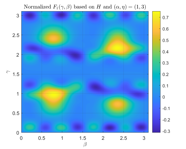
(b) $(\alpha,\eta)=(1,3)$.

​​ 

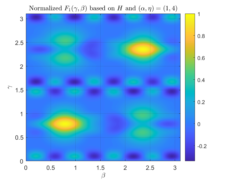
(c) $(\alpha,\eta)=(1,4)$.

​​  

(d) $(\alpha,\eta)=(1,5)$.

Figure 1: Normalized expectation $F_{1}$ for the cost Hamiltonian defined by $H_{[7,4,3]}$ and various combinations of $(\alpha,\eta)$ with syndrome zero.

V.1.1 Using a full-rank parity-check matrix

Consider the cost Hamiltonian defined by $H_{[7,4,3]}$, $\alpha=1,\,\eta=4$, and some ${\bm{s}}\in\{0,1\}^{3}$ and sufficiently large $T$. From numerous simulations, we conclude that optimization over the angles $\bm{\beta}$ and $\bm{\gamma}$ by NM+basin-hopping or COBYLA+multistart will have better numerical results.

For NM+basin-hopping, we additionally test four starting points with $(\gamma_{p},\beta_{p})=(0,0)$, $(\frac{\pi}{8},\frac{\pi}{8})$, $(1,1)$ or at random, and choose the one that has the largest mean objective $F_{p}$. For COBYLA+multistart, each angle $\gamma_{j}$ or $\beta_{j}$ has possible $\kappa$ values, so a total of $\kappa^{2p}$ starting points are tested. However, we choose different values of $\kappa$ such that $\kappa^{2p}\leq 256$. We do these optimizations for each syndrome ${\bm{s}}$. The results are shown in Fig. 2, where $\operatorname{avg}_{\bm{s}}F_{p}$ denotes the mean expectation value $F_{p}$ averaged over all ${\bm{s}}\in\{0,1\}^{3}$ and $\min_{\bm{s}}F_{p}$ denotes the worst result of the tested syndromes. (The value $\min_{\bm{s}}F_{p}$ is the expectation value corresponding to the cost Hamiltonian of some error syndrome that is the most difficult for the QAOA.) One can see that NM+basin-hopping performs slightly better than COBYLA+multistart.

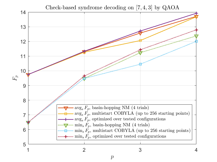
Figure 2: Simulated $F_{p}$ for check-based syndrome decoding of the classical $[7,4,3]$ Hamming code by OAQA.

The complete QAOA decoding of the $[7,4,3]$ code is as follows. An error ${\bm{e}}\in\{0,1\}^{n}$ is generated according to an independent binary symmetric channel (BSC) with cross error rate $\epsilon$. If the syndrome of the error is zero, the decoding output is $\hat{\bm{e}}=\bm{0}$. Otherwise, we simulate Algorithm 3 for a certain $T$ with $(\bm{\gamma},\bm{\beta})$ determined by the better optimization method as mentioned above. Upon receiving an output distribution together with $T$ possible errors, the error of minimum weight that matches the error syndrome will be returned as the output $\hat{{\bm{e}}}$. If there are no errors matching the syndrome, the decoding output is chosen to be $\hat{\bm{e}}=\bm{0}$. A decoding error occurs if $\hat{\bm{e}}\neq{\bm{e}}$.

In our simulations, unless otherwise specified, 500 decoding errors are collected. The performance of QAOA decoding on the $[7,4,3]$ code is shown in Fig. 3 for several levels $p$ and iteration numbers $T$. Since the $[7,4,3]$ code is perfect, the maximum-likelihood decoding rule is equivalent to the bounded-distance decoder (BDD) with block error rate

$$P_{\rm e,BDD}(n,d)=1-\textstyle\sum_{~{}j=0}^{\lfloor\frac{d-1}{2}\rfloor}\binom{n}{j}\epsilon^{j}(1-\epsilon)^{n-j}$$ (29)

at cross error rate $\epsilon$. This is also plotted in Fig. 3.

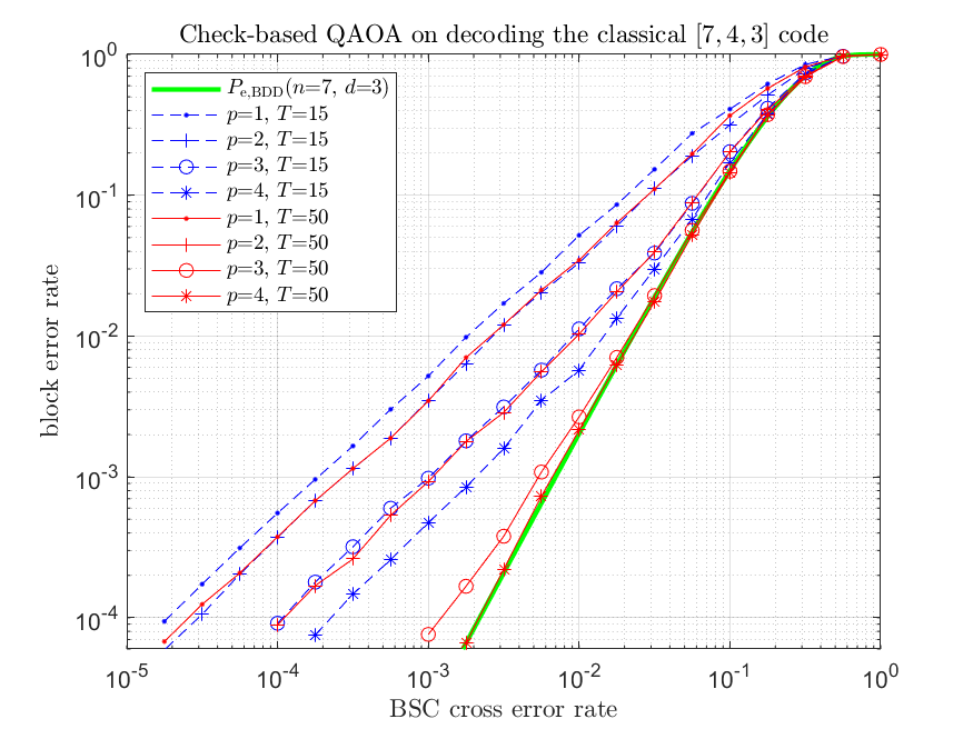
Figure 3: The performance of check-based syndrome decoding on the classical $[7,4,3]$ code by OAQA using $H_{[7,4,3]}$.

For $T=15$, the block error rate is less than the cross error rate when $p\geq 4$ so that the advantage of coding can be observed. For $T=50$, the QAOA decoder matches the performance of the BDD when $p\geq 4$.

V.1.2 Improvement with redundant clauses

In this subsection, we show that QAOA decoding can be improved with an modified cost Hamiltonian that defines an equivalent decoding problem without any cost. More precisely, we may introduce redundant clauses but the number of qubits remains the same. Note that this technique can be applied to either the check-based or the generator-based decoding. We demonstrate this on the decoding of the $[7,4,3]$ code again.

The $[7,4,3]$ code has an equivalent code with a parity-check matrix that can be cyclicly generated by a row vector $(1,0,1,1,1,0,0)$ as

$$H^{\text{(circ)}}=\left[\begin{smallmatrix}1&0&1&1&1&0&0\\ 0&1&0&1&1&1&0\\ 0&0&1&0&1&1&1\\ 1&0&0&1&0&1&1\\ 1&1&0&0&1&0&1\\ 1&1&1&0&0&1&0\\ 0&1&1&1&0&0&1\end{smallmatrix}\right].$$ (30)

Note that $H^{\text{(circ)}}$ is of rank $3$. One can see that $H^{\text{(circ)}}$ provides equal protection capability on each bit. Consequently the cost Hamiltonian defined according to $H^{\text{(circ)}}$ has a circulant symmetry. By a similar argument as for Eq. (28), we consider $(\alpha,\eta)=(1,1)$ or $(2,3)$. As shown in Fig. 4, we choose $(\alpha,\eta)=(1,1)$, whose energy topology is smoother and its maximum normalized value is one.

​​​​​

(a) $(\alpha,\eta)=(1,1)$.

​​​

(b) $(\alpha,\eta)=(2,3)$.

Figure 4: Normalized expectation $F_{1}$ for the cost Hamiltonian defined by $H^{\text{(circ)}}$ and $(\alpha,\eta)=(1,1)$ or $(2,3)$ with syndrome zero.

As in the previous subsection, we use NM+basin-hopping and COBYLA+multistart to optimize $F_{p}$ over $(\bm{\gamma},\bm{\beta})$ for $p=1,\dots,4$ for different syndromes and the normalized $F_{p}$ are shown in Fig. 5. We plot also the optimized curves in Fig. 2 by the non-circulant matrix $H_{[7,4,3]}$ for comparison. The performance is significantly improved such that $\min_{{\bm{s}}}F_{p}$ by $H^{\text{(circ)}}$ is comparable to $\text{avg}_{{\bm{s}}}\,F_{p}$ by $H_{[7,4,3]}$.

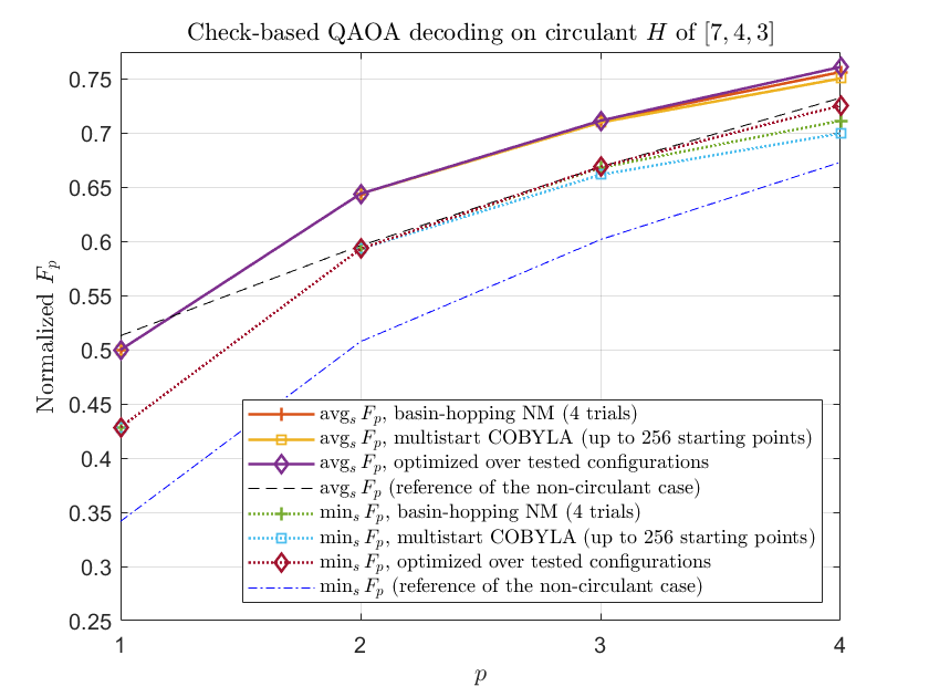
Figure 5: Simulated $F_{p}$ for check-based syndrome decoding on the $[7,4,3]$ Hamming code using the circulant parity-check matrices $H^{\text{(circ)}}$ or the non-circulant $H_{[7,4,3]}$.

The decoding performance of Algorithm 3 based on $H^{\text{(circ)}}$ and optimized $(\bm{\gamma},\bm{\beta})$ is shown in Fig. 6. The decoding gain appears for $T=5$ and the BBD performance is achieved for $T=15$. These significantly improve the results in Fig. 3.

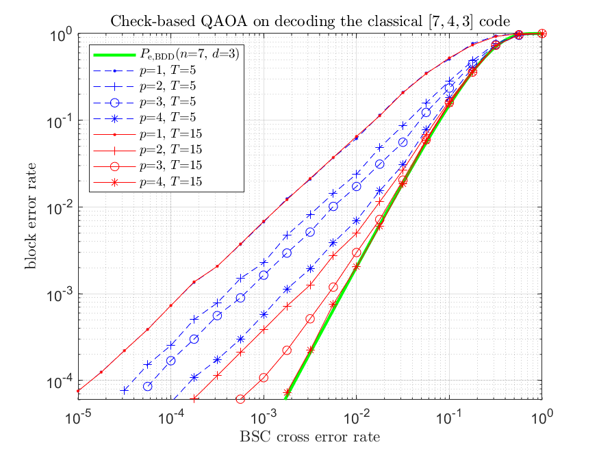
Figure 6: The performance of check-based syndrome decoding on the classical $[7,4,3]$ code by OAQA using $H^{\text{(circ)}}$.

V.2 Decoding quantum codes by QAOA

In this section, we simulate QAOA decoding on the $[[5,1,3]]$ and $[[9,1,3]]$ quantum codes. Algorithm 4 needs $n+k$ qubits to decode an $[[n,k]]$ code, while Algorithm 5 needs $2n$ qubits. We simulate only Algorithm 4 in this section.

V.2.1 The $[[5,1,3]]$ code

The $[[5,1,3]]$ code has been discussed in Example 3. We consider the generator-based decoding Algorithm 4 with the following generator matrices

(43)

Note that $G_{\mathcal{S}}^{\prime}$ defines the same code as $G_{\mathcal{S}}$ does but $G_{\mathcal{S}}^{\prime}$ has fewer 1’s in the last two rows. As in the previous subsection, we use NM+basin-hopping and COBYLA+multistart to optimize $F_{p}$ over $(\bm{\gamma},\bm{\beta})$ for $p=1,\dots,4$ for different syndromes and the normalized $F_{p}$ are shown in Fig. 7.

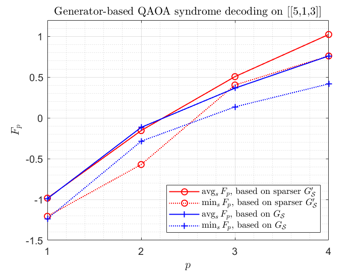
Figure 7: Simulated $F_{p}$ for generator-based decoding on the $[[5,1,3]]$ code by QAOA using $G_{\mathcal{S}}$ and $G_{\mathcal{S}}^{\prime}$.

The complete QAOA decoding of a quantum code is as follows. An error ${\bm{e}}\in\{0,1\}^{2n}$ is generated according to an independent depolarizing channel of rate $\epsilon$ with probability

$$P_{\text{dep}}({\bm{e}})=(\epsilon/3)^{\text{gw}\left({\bm{e}}\right)}(1-\epsilon)^{n-\text{gw}\left({\bm{e}}\right)}.$$ (44)

If the syndrome of the error is zero, the decoding output is $\hat{\bm{e}}=\bm{0}$. Otherwise, we simulate Algorithm 4 for a certain $T$ with $(\bm{\gamma},\bm{\beta})$ determined by the better optimization method. Upon receiving an output distribution together with $T$ possible errors, the error of minimum generalized weight that matches the error syndrome will be returned as the output $\hat{{\bm{e}}}$. If there are no errors matching the syndrome, the decoding output is chosen to be $\hat{\bm{e}}=\bm{0}$. A decoding (logical) error occurs if and only if $\hat{\bm{e}}$ is not a degenerate error of ${\bm{e}}$. Thus there are $2^{4}$ valid solutions.

We simulate the decoding performance of Algorithm 4 by collecting 500 decoding errors for each data point, and the results are shown in Fig. 8. The $[[5,1,3]]$ code is a perfect code so we compare our QAOA decoding with the BDD performance. The BDD performance is also shown in the plot ($P_{\rm e,BDD}$ for reference). As expected, the performance is better using a sparser matrix $G_{\mathcal{S}}^{\prime}$. For depolarizing rate roughly larger than $0.3$, the logical error rate of QAOA decoder can be better than the BDD performance because of degeneracy. (See [RW05] and [KL21, Fig. 9] for more discussions about the performance of $[[5,1,3]]$ in this region.)

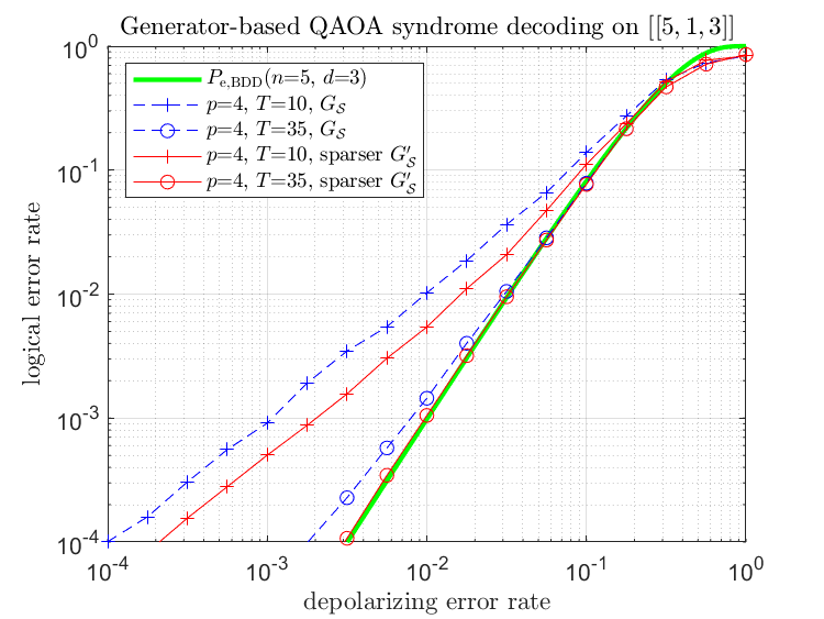
Figure 8: The performance of generator-based syndrome decoding on the $[[5,1,3]]$ code by QAOA.

V.2.2 Output distribution by the QAOA decoder

When the number of qubits in a $p$-level QAOA is large, classical simulations of all the syndromes are difficult for $p\geq 2$. Thus we may instead focus on the output distribution of Algorithm 4 for a particular syndrome ${\bm{s}}$ to analyze its resemblance to the real distribution.

Let ${\bm{z}}_{\bm{s}}\in\{0,1\}^{2n}$ be a vector with syndrome ${\bm{s}}$. Then the occurred error must be of the form ${\bm{u}}G_{\mathcal{S}}+{\bm{z}}_{\bm{s}}$ for some ${\bm{u}}\in\{0,1\}^{n+k}$. The conditional probability of ${\bm{u}}$ given ${\bm{s}}$ is

$$P({\bm{u}}|{\bm{s}})=\frac{P_{\text{dep}}({\bm{u}}G_{\mathcal{S}}+{\bm{z}}_{\bm{s}})}{\sum_{{\bm{v}}\in\{0,1\}^{n+k}}P_{\text{dep}}({\bm{v}}G_{\mathcal{S}}+{\bm{z}}_{\bm{s}})},$$ (45)

where $P_{\text{dep}}$ is defined in Eq. (44). Let $Q({\bm{u}}|{\bm{s}})$ denote the conditional distribution output by the QAOA decoder. We may evaluate the similarity of $P({\bm{u}}|{\bm{s}})$ and $Q({\bm{u}}|{\bm{s}})$ using the Jensen–Shannon (JS) divergence [ES03]

$$J(P\|Q)=\tfrac{1}{2}D(P\|M)+\tfrac{1}{2}D(Q\|M),$$

where $M=\frac{1}{2}(P+Q)$ and $D(P\|Q)=\sum_{{\bm{u}}\in\{0,1\}^{n+k}}P({\bm{u}}|{\bm{s}})\log\frac{P({\bm{u}}|{\bm{s}})}{Q({\bm{u}}|{\bm{s}})}$ is the Kullback–Leibler (KL) divergence [KL51]. The value of JS divergence is bounded in $[0,1]$ and its value is close to zero for two similar distributions.

Consider the syndrome of $\hat{X}_{1}$ (or ${\bm{e}}=(10000|00000)$) and ${\bm{z}}_{\bm{s}}=(10000|00000)$. The approximation by QAOA using the $G^{\prime}_{\mathcal{S}}$ in Eq. (LABEL:eq:G_513) is given in Fig. 9, with $P$ also plotted for reference. We find that $J(P\|Q)=0.06658$ at depolarizing rate $\epsilon=0.32$ when $Q$ is the output distribution of the $4$-level QAOA decoder, as shown in Fig. 9. Note that

$$({\bm{u}})_{10}=\textstyle\sum_{i}u_{i}2^{i}$$

is the decimal representation of ${\bm{u}}=(u_{1},u_{2},\dots,u_{n+k})\in\{0,1\}^{n+k}$. In this case $\varphi(\hat{X}_{1})$ corresponds to $({\bm{u}})_{10}=0$.

To approximate the distribution $P$ is computationally hard. Similarly, we have $J(P\|Q)=0.1146$ for the syndrome of $\hat{Y}_{1}$ at $\epsilon=0.38$ as shown in Fig. 10. The approximation is not as good as the previous one.

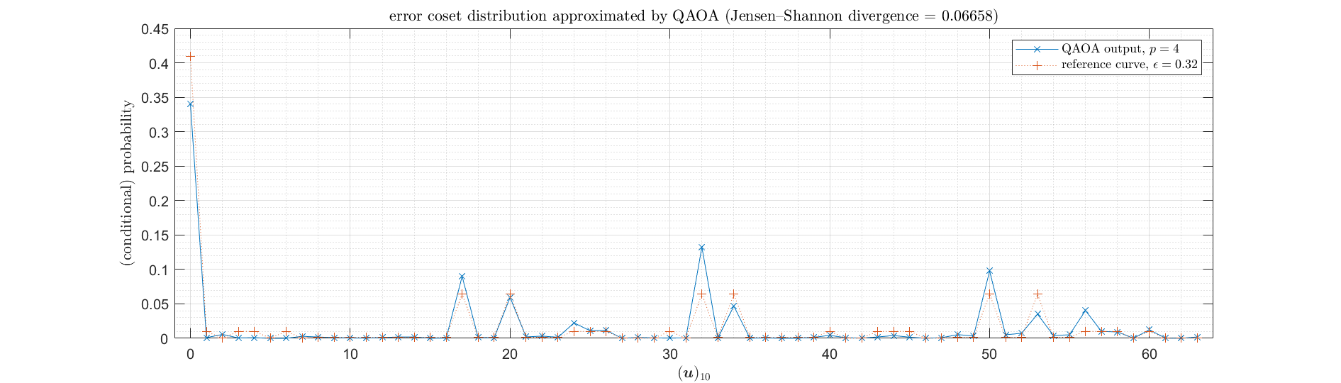
Figure 9: The output distribution of the $4$-level QAOA decoding on the $[[5,1,3]]$ code by Algorithm 4, given the syndrome of $\hat{X}_{1}$.

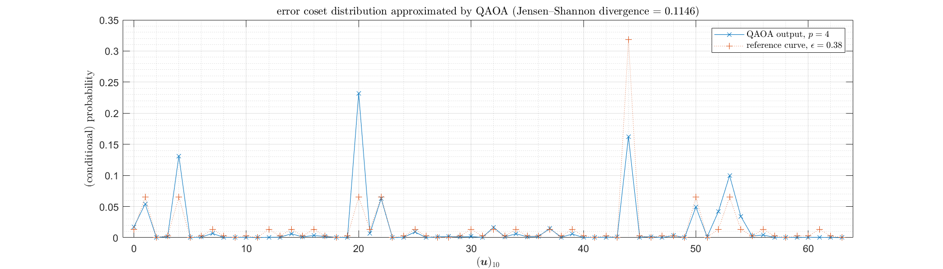
Figure 10: The output distribution of the $4$-level QAOA decoding on the $[[5,1,3]]$ code by Algorithm 4, given the syndrome of $\hat{Y}_{1}$.

V.2.3 Shor’s $[[9,1,3]]$ code

Next we study the QAOA decoding on Shor’s $[[9,1,3]]$ code [Shor95], which is a degenerate code. It has a generator matrix Eq. (19) as