Application of Hawkes volatility in the observation of filtered high-frequency price process in tick structures

Abstract

The Hawkes model is suitable for describing self and mutually exciting random events. In addition, the exponential decay in the Hawkes process allows us to calculate the moment properties in the model. However, due to the complexity of the model and formula, few studies have been conducted on the performance of Hawkes volatility. In this study, we derived a variance formula that is directly applicable under the general settings of both unmarked and marked Hawkes models for tick-level price dynamics. In the marked model, the linear impact function and possible dependency between the marks and underlying processes are considered. The Hawkes volatility is applied to the mid-price process filtered at 0.1-second intervals to show reliable results; furthermore, intraday estimation is expected to have high utilization in real-time risk management. We also note the increasing predictive power of intraday Hawkes volatility over time and examine the relationship between futures and stock volatilities.

1 Introduction

The importance of volatility as a risk measure of financial assets was first observed by Markowitz (1952). Since then, research on the historical volatility of financial asset prices has progressed. For example, seminal studies on volatility were conducted via autoregressive heteroscedastic models, proposed by Engle (1982) and Bollerslev (1986), which typically estimates the volatilities based on daily data. Daily data as well as intraday data have become useful for volatility estimation with the development of computing, recording, and storage technology, thereby advancing the theory and practice of volatility estimation.

Based on the theory of quadratic variation of semimartingales, the realized volatility studied by Andersen et al. (2003), which is equivalent to the integrated volatility (Barndorff-Nielsen and Shephard, 2002a, b) for the Itô process, is a reliable estimator of volatility; it uses intraday data observed at appropriate frequencies. These theories and practical application methodologies were further developed by Barndorff-Nielsen and Shephard (2004), Aït-Sahalia et al. (2005), Zhang et al. (2005), Hansen and Lunde (2006) and Aït-Sahalia et al. (2011).

Another useful methodology for volatility estimation using intraday data is based on point processes. The Hawkes process, a type of point process introduced by (Hawkes, 1971a) and (Hawkes, 1971b), was initially recognized for its importance in seismology; however, it has been used in various fields such as finance, biology, and computer science since.

Early studies that applied the Hawkes model in the field of finance include Hewlett (2006), Bowsher (2007), and Large (2007). The Hawkes point process or similar intensity-based models have been studied in terms of price dynamics, especially for microstructure, (Bauwens and Hautsch, 2009; Bacry and Muzy, 2014; Blanc et al., 2017), bid-ask price (Lee and Seo, 2022) and limit order book modeling (Zheng et al., 2014; Hainaut and Goutte, 2019; Morariu-Patrichi and Pakkanen, 2021), with various applications such as optimal execution (Choi et al., 2021; Da Fonseca and Malevergne, 2021). It has also been used in other financial studies on credit risk (Errais et al., 2010; Dassios and Zhao, 2012; Aït-Sahalia et al., 2015), extreme risk (Herrera and Clements, 2018), and systemic risk (Jang et al., 2020). The theoretical and applied studies on the Hawkes process in finance were reviewed by Law and Viens (2015), Bacry et al. (2015), and Hawkes (2018).

In this study, we compute the daily and intraday volatility of financial asset prices based on the Hawkes models. Under the mutually and self-excited non-marked Hawkes model framework, Bacry et al. (2013) derived the formulas for the signature plot and correlation of two price increments. A similar result was found in Da Fonseca and Zaatour (2014a), under a non-marked Hawkes model setting, with derivations in matrix forms and linear differential equations. Further, Lee and Seo (2017b) focused on the volatility estimation under the symmetric setting in the Hawkes kernel. The result of a similar calculation for the general moments of the Hawkes model is demonstrated step-by-step in Cui et al. (2020).

An extension of the basic Hawkes modeling of financial data can be achieved through the consideration of the size of the event. The marked Hawkes model is extended by including the magnitude of the event or the size of the jump in the model. An early study on the application of the marked model to financial data can be found in Embrechts et al. (2011). Lee and Seo (2017a) further attempted to estimate volatility under the marked Hawkes process. Our study can be viewed as an extended version with more relaxed parameter conditions. Further, the marked Hawkes processes have been actively studied in the field of finance by Chavez-Demoulin and McGill (2012), Ji et al. (2020), and Cai (2020).

Our first goal is to propose a closed-form volatility formula that can be used directly in computer programs, under minimal model assumptions and parameter constraints. The volatility formula is derived for all non-mark, dependent mark, and independent mark models, and provides a closed-form solution under minimal assumptions. Volatility can be computed using the estimates based on the high-frequency stock price data and our empirical study showed stable results.

Second, we can test the performance of Hawkes volatility through model estimation. For model estimation, we did not use raw data that recorded all the activities but rather used filtered data at 0.1 second intervals. The filtered data removes rather meaningless information in ultra-high frequency level, making it easier to compute long-term; for example, daily volatility. The result shows that the Hawkes volatility showed high performance with increasing predictive power over time. A comparison study with realized volatility is also provided.

In addition, the abundance of tick data makes it possible to measure Hawkes volatility in real time, which is a huge advantage of Hawkes volatility. Real time Hawkes variability enables detailed empirical analysis. For example, we visualize the pattern in which the inflow information contributes to the prediction of volatility as new information flows into the market. We also examine the relationship and predictability between futures and stock market volatilities for denser time intervals.

The remainder of the paper is structured as follows. Section 2 introduces the basic unmarked Hawkes model and derives the volatility formula. Section 3 extends the results to the marked Hawkes model. Section 4 shows the various empirical results with their estimation. Section 5 concludes the study. The proofs are gathered in the A and example estimation result can be found in B.

2 Basic Hawkes model

The microstructure of stock price dynamics at the intraday level can be described by two-point processes $N_{i}$ for $i=1,2$, which represent the times of up ($i=1$) and down ($i=2$) price movements, respectively. In this section, we derive the formula of

$$\mathrm{Var}(N_{1}(t)-N_{2}(t))$$ (1)

which measures the variability of price changes under the condition that $N_{1}$ and $N_{2}$ follow the Hawkes processes with $N_{1}(0)=N_{2}(0)=0$. Accordingly, we derive the formulas for the moments of the intensity and counting processes of the basic bivariate Hawkes model in terms of parameters. The basic Hawkes model for intraday price dynamics does not include marks, which can be used to describe the jump size or trade volume in microstructure price movements. Thus, the basic Hawkes model only describes the distribution of the size of the intervals between events.

The derivation for the moments in the basic Hawkes model is not entirely a new approach; similar findings can be found in previous studies. Under a similar setting, Da Fonseca and Zaatour (2014b) derived the differential equations for moments. Lee and Seo (2017b) derived the daily Hawkes volatility formula with a symmetric kernel. Cui et al. (2020) presented an approach to obtain the moments of Hawkes processes and intensities. We review them in an organized manner to derive Eq. (1). Hence the formula can be used practically; for example, it can be applied directly in a computer programming code. Deriving the variance formula of the basic Hawkes model is important because it serves as a building block for the derivation of the volatility formula in more complicated models.

The basic Hawkes process is defined in a probability space $(\Omega,\mathcal{F},\mathbb{P})$. There is a strictly increasing sequence of real-valued random variables $\{\tau_{i,n}\}$, which represent the event times, on the space with countable index $n$. Assuming simple counting processes, the probability of two or more events occurring at the same time is zero. For practical purposes, only positive $\tau$s are meaningful, however, to define the intensity processes later, non-positive $\tau$s are assumed to also exist conceptually.

We use $N_{i}$ to denote the counting process as a stochastic process, and a random measure,

$$N_{i}(t)=N_{i}((0,t])=\sum_{n}\mathbbm{1}_{\{0<\tau_{i,n}\leq t\}}=\#\textrm{ of }\tau_{i,n}\in(0,t],\quad\textrm{for }i=1,2.$$

The stochastic intensity $\lambda_{i}$ of the given counting process $N_{i}$ is a non-negative and $\mathcal{F}$-predictable process such that

$$\mathbb{E}\left[\left.\int_{s}^{t}\lambda_{i}(u)\mathrm{d}u\right|\mathcal{F}_{s}\right]=\mathbb{E}[N_{i}(t)-N_{i}(u)|\mathcal{F}_{s}],\quad\textrm{for }s<t.$$

The bivariate Hawkes processes and their corresponding intensity processes are defined by

$$\bm{N}_{t}=\begin{bmatrix}N_{1}(t)\\ N_{2}(t)\end{bmatrix},\quad\bm{\lambda}_{t}=\begin{bmatrix}\lambda_{1}(t)\\ \lambda_{2}(t)\end{bmatrix},$$

where

$$\bm{\lambda}_{t}=\bm{\mu}+\int_{-\infty}^{t}\bm{h}(t-u)\mathrm{d}\bm{N}_{u}$$ (2)

with the matrix-vector multiplication in the integral; $\bm{\mu}=[\mu_{1},\mu_{2}]^{\top}$ is a positive constant vector representing the exogenous intensities; $\bm{h}$ is often called a kernel, such that

$$\bm{h}(t)=\bm{\alpha}\circ\begin{bmatrix}\mathrm{e}^{-\beta_{1}t}&\mathrm{e}^{-\beta_{1}t}\\ \mathrm{e}^{-\beta_{2}t}&\mathrm{e}^{-\beta_{2}t}\end{bmatrix}$$

with the Hadamard (element-wise) product $\circ$; $\bm{\alpha}$ is a positive $2\times 2$ constant matrix. The order of the Hadamard product $\circ$ and the matrix product is from left to right. Note that $\bm{\mu}$ and $\bm{\alpha}$ have no parameter restrictions; however, the decay rates $\beta$s have the same value for each $i$ to ensure the Markov property of joint process $(\bm{N},\bm{\lambda})$.

In a differential form, the intensity vector process is represented by

$$\mathrm{d}\bm{\lambda}_{t} =\bm{\beta}(\bm{\mu}-\bm{\lambda}_{t})\mathrm{d}t+\bm{\alpha}\mathrm{d}\bm{N}_{t}$$

$$=\{\bm{\beta}\bm{\mu}+(\bm{\alpha}-\bm{\beta})\bm{\lambda}_{t})\}\mathrm{d}t+\bm{\alpha}(\mathrm{d}\bm{N}_{t}-\bm{\lambda}_{t}\mathrm{d}t),$$

where

$$\bm{\beta}=\begin{bmatrix}\beta_{1}&0\\ 0&\beta_{2}\end{bmatrix},$$

is a diagonal matrix. In an integral form,

$$\bm{\lambda}_{t}={} \bm{\lambda}_{0}+\int_{0}^{t}\bm{\beta}(\bm{\mu}-\bm{\lambda}_{s})\mathrm{d}s+\int_{0}^{t}\bm{\alpha}\mathrm{d}\bm{N}_{s}$$ (3)

$$={} \bm{\lambda}_{0}+\int_{0}^{t}\{\bm{\beta}\bm{\mu}+(\bm{\alpha}-\bm{\beta})\bm{\lambda}_{s})\}\mathrm{d}s+\int_{0}^{t}\bm{\alpha}(\mathrm{d}\bm{N}_{s}-\bm{\lambda}_{s}\mathrm{d}s),$$ (4)

where the last term in Eq. (4) is a martingale. The counting processes are right continuous, and the intensity processes are left continuous. If the spectral radius of

$$\left|\int_{0}^{\infty}\bm{h}(t)\mathrm{d}t\right|,$$

is less than 1, it is known that $\bm{N}$ has a unique stationary version. By conditioning the Hawkes process to begin at $-\infty$, we always assume that the unconditional distribution of the intensity processes at and after time 0 will no longer change. Therefore, we always assume that $\bm{\lambda}$ is in a steady state at time 0. Hence the unconditional joint distribution of $(\lambda_{1}(s),\lambda_{2}(s))$ and $(\lambda_{1}(t),\lambda_{2}(t))$ are identical for any time $s,t\geq 0$.

The following formula is well known.

Proposition 1.

Under the steady state assumption,

$$\mathbb{E}[\bm{\lambda}_{t}]=(\bm{\beta}-\bm{\alpha})^{-1}\bm{\beta}\bm{\mu}=\left(\bm{\mathrm{I}}-\bm{\beta}^{-1}\bm{\alpha}\right)^{-1}\bm{\mu}.$$ (5)

To proceed further, we use the concept of the quadratic (co)variation of semimartingales in a matrix version. Consider the vectors of semimartingale processes $\bm{X}$ and $\bm{Y}$. The integration by parts of $\bm{X}_{t}\bm{Y}^{\top}_{t}$ is represented in a differential form

$$\mathrm{d}(\bm{X}_{t}\bm{Y}^{\top}_{t}) =\bm{X}_{t-}\mathrm{d}\bm{Y}^{\top}_{t}+\mathrm{d}(\bm{X}_{t})\bm{Y}^{\top}_{t-}+\mathrm{d}[\bm{X}\bm{Y}^{\top}]_{t},$$ (6)

where $\mathrm{d}(\bm{X}_{t})\bm{Y}^{\top}_{t-}$ implies $(\bm{Y}_{t-}\mathrm{d}\bm{X}_{t}^{\top})^{\top}$ and $[\bm{X}\bm{Y}^{\top}]_{t}$ denotes the matrix whose elements are the quadratic (co)variations for the entries of $\bm{X}_{t}\bm{Y}_{t}^{\top}$.

Notation 1.

If $\bm{\mathrm{x}}$ is a vector, then $\mathrm{Dg}(\bm{\mathrm{x}})$ denotes a diagonal matrix whose diagonal entries are composed of the elements of $\bm{\mathrm{x}}$. If $\bm{\mathrm{M}}$ is a square matrix, then $\mathrm{Dg}(\bm{\mathrm{M}})$ denotes a diagonal matrix whose diagonal entries are the diagonal part of $\bm{\mathrm{M}}$. In addition, let $\mathcal{T}$ be an operator, such that

$$\mathcal{T}(\bm{\mathrm{M}})=\bm{\mathrm{M}}+\bm{\mathrm{M}}^{\top}$$

for a square matrix $\bm{\mathrm{M}}$.

Lemma 2.

Consider $2\times 1$ vector processes $\bm{X}$ and $\bm{Y}$ such that

$$\mathrm{d}\bm{X}_{t}=\bm{a}_{t}\mathrm{d}t+\bm{f}_{x}(t)\mathrm{d}\bm{N}_{t},\quad\mathrm{d}\bm{Y}_{t}=\bm{b}_{t}\mathrm{d}t+\bm{f}_{y}(t)\mathrm{d}\bm{N}_{t}$$

where $\bm{a}$ and $\bm{b}$ are $2\times 1$ vector processes, and $\bm{f}_{x}$ and $\bm{f}_{y}$ are $2\times 2$ matrix processes. Then

$$\mathrm{d}[\bm{X}\bm{Y}^{\top}]_{t}=\bm{f}_{x}(t)\mathrm{Dg}(\mathrm{d}\bm{N}_{t})\bm{f}_{y}^{\top}(t).$$

Thus, by Eq. (6),

$$\mathrm{d}(\bm{X}_{t}\bm{Y}^{\top}_{t}) =\bm{X}_{t-}\mathrm{d}\bm{Y}^{\top}_{t}+\mathrm{d}(\bm{X}_{t})\bm{Y}^{\top}_{t-}+\bm{f}_{x}(t)\mathrm{Dg}(\mathrm{d}\bm{N}_{t})\bm{f}_{y}^{\top}(t).$$

In addition, when $\mathbb{E}[\bm{X}_{t}\bm{Y}^{\top}_{t}]$ exists,

$$\frac{\mathrm{d}\mathbb{E}[\bm{X}_{t}\bm{Y}^{\top}_{t}]}{\mathrm{d}t}=\mathbb{E}[\bm{X}_{t-}(\bm{b}_{t}^{\top}+\bm{\lambda}_{t}^{\top}\bm{f}_{y}^{\top}(t))]+\mathbb{E}[(\bm{a}_{t}+\bm{f}_{x}(t)\bm{\lambda}_{t})\bm{Y}^{\top}_{t-}]+\bm{f}_{x}(t)\mathrm{Dg}(\mathbb{E}[\bm{\lambda}_{t}])\bm{f}_{y}^{\top}(t).$$

Proposition 3.

We have the following Sylvester equation for $\mathbb{E}[\bm{\lambda}_{t}\bm{\lambda}_{t}^{\top}]$:

$$\mathbb{E}[\bm{\lambda}_{t}\bm{\lambda}_{t}^{\top}](\bm{\alpha}-\bm{\beta})^{\top}+(\bm{\alpha}-\bm{\beta})\mathbb{E}[\bm{\lambda}_{t}\bm{\lambda}_{t}^{\top}]+\mathbb{E}[\bm{\lambda}_{t}](\bm{\beta}\bm{\mu})^{\top}+\bm{\beta}\bm{\mu}\mathbb{E}[\bm{\lambda}_{t}^{\top}]+\bm{\alpha}\mathrm{Dg}(\mathbb{E}[\bm{\lambda}_{t}])\bm{\alpha}^{\top}=\bm{0}$$ (7)

or using the Notation 1,

$$\mathcal{T}\left((\bm{\alpha}-\bm{\beta})\mathbb{E}[\bm{\lambda}_{t}\bm{\lambda}_{t}^{\top}]+\bm{\beta}\bm{\mu}\mathbb{E}[\bm{\lambda}_{t}^{\top}]\right)+\bm{\alpha}\mathrm{Dg}(\mathbb{E}[\bm{\lambda}_{t}])\bm{\alpha}^{\top}=\bm{0}$$

where $\bm{0}$ denotes the $2\times 2$ zero matrix and $\mathbb{E}[\bm{\lambda}_{t}$ satisfies Eq. (5).

Solving the above Sylvester equation in Eq. (7) is equivalent to solving:

$$\{\bm{\mathrm{I}}\otimes(\bm{\alpha}-\bm{\beta})+(\bm{\alpha}-\bm{\beta})\otimes\bm{\mathrm{I}}\}\mathrm{vec}\left(\mathbb{E}[\bm{\lambda}_{t}\bm{\lambda}_{t}^{\top}]\right)=-\mathrm{vec}\left(\mathbb{E}[\bm{\lambda}_{t}](\bm{\beta}\bm{\mu})^{\top}+\bm{\beta}\bm{\mu}\mathbb{E}[\bm{\lambda}_{t}^{\top}]+\bm{\alpha}\mathrm{Dg}(\mathbb{E}[\bm{\lambda}_{t}])\bm{\alpha}^{\top}\right)$$

where $\otimes$ denotes the Kronecker product and $\mathrm{vec}$ is the vectorization operator. By assuming the steady state condition, the first and second moments of $\lambda$s do not depend on the time; however, $\mathbb{E}[\bm{\lambda}_{t}\bm{N}_{t}^{\top}]$ depends on time.

Proposition 4.

For $\mathbb{E}[\bm{\lambda}_{t}\bm{N}_{t}^{\top}]$, we have the following first order $2\times 2$ system of differential equation:

$$\frac{\mathrm{d}\mathbb{E}[\bm{\lambda}_{t}\bm{N}_{t}^{\top}]}{\mathrm{d}t}=(\bm{\alpha}-\bm{\beta})\mathbb{E}[\bm{\lambda}_{t}\bm{N}_{t}^{\top}]+\bm{\beta}\bm{\mu}\mathbb{E}[\bm{\lambda}_{t}^{\top}]t+\mathbb{E}[\bm{\lambda}_{t}\bm{\lambda}_{t}^{\top}]+\bm{\alpha}\mathrm{Dg}(\mathbb{E}[\bm{\lambda}_{t}]).$$

Let $\bm{\mathrm{V}}=\begin{bmatrix}\bm{\mathrm{v}}_{1}&\bm{\mathrm{v}}_{2}\end{bmatrix}$ be the eigenvector matrix of $\bm{\alpha}-\bm{\beta}$ and $\xi_{1}$ and $\xi_{2}$ are corresponding eigenvalues. The solution of the system is

$$\mathbb{E}[\bm{\lambda}_{t}\bm{N}_{t}^{\top}]=\bm{\mathrm{V}}\bm{\mathrm{C}}\circ\begin{bmatrix}\mathrm{e}^{\xi_{1}t}&\mathrm{e}^{\xi_{1}t}\\ \mathrm{e}^{\xi_{2}t}&\mathrm{e}^{\xi_{2}t}\end{bmatrix}+\bm{\mathrm{A}}t+\bm{\mathrm{B}}$$

where

$$\bm{\mathrm{A}} =-(\bm{\alpha}-\bm{\beta})^{-1}\bm{\beta}\bm{\mu}\mathbb{E}[\bm{\lambda}_{t}^{\top}]=\mathbb{E}[\bm{\lambda}_{t}]\mathbb{E}[\bm{\lambda}_{t}]^{\top}$$ (8)

$$\bm{\mathrm{B}} =(\bm{\alpha}-\bm{\beta})^{-1}\{\bm{A}-\mathbb{E}[\bm{\lambda}_{t}\bm{\lambda}_{t}^{\top}]-\bm{\alpha}\mathrm{Dg}(\mathbb{E}[\bm{\lambda}_{t}])\}$$ (9)

and $\bm{\mathrm{C}}$ is a constant coefficient matrix that satisfies the initial condition:

$$\mathbb{E}[\bm{\lambda}_{0}\bm{N}_{0}^{\top}]=\bm{0}.$$

As $t\rightarrow\infty$, only the particular solution is significant, that is,

$$\mathbb{E}[\bm{\lambda}_{t}\bm{N}_{t}^{\top}]\approx\bm{\mathrm{A}}t+\bm{\mathrm{B}}.$$

Note that, even if we assume that $\bm{\lambda}$ is in a steady state at time 0, $\mathbb{E}[\bm{\lambda}_{t}\bm{N}_{t}^{\top}]$ has an exponentially converging term. However, the homogeneous solution of the exponential is rather insignificant with a relatively large $t$ under the condition that the spectral radius is less than 1; hence $\mathbb{E}[\bm{\lambda}_{t}\bm{N}_{t}^{\top}]$ can be approximated as an affine form of time $t$. With this approximation, the variance of the net number of up and down between 0 and $t$ is presented below. To compute the variance of price change, the formula should be adjusted based on the minimum tick size.

Theorem 5.

We have

$$\mathrm{Var}(N_{1}(t)-N_{2}(t)) \approx\bm{\mathrm{u}}^{\top}\left(2\bm{\mathrm{B}}+\mathrm{Dg}(\mathbb{E}[\bm{\lambda}_{t}])\right)\bm{\mathrm{u}}t$$

where $\bm{\mathrm{B}}$ is defined by Eq. (9) and $\bm{\mathrm{u}}=\begin{bmatrix}1&-1\end{bmatrix}^{\top}.$

3 Marked model

In this section, we introduce a marked Hawkes model that incorporates both the timing and size of the asset price movement. This section can be regarded as the general version of Lee and Seo (2017a). As in the previous section with a non-marked model, we present the variance formula of the marked Hawkes model. The marked model differs from the non-marked model in two ways. First, the effect of jump size on future intensity should be considered. Second, the possibility of dependence between the jump size and other underlying processes, such as $\bm{\mathrm{N}}$ and $\bm{\lambda}$, should be considered.

For $i=1,2$, let

$$E_{i}=\mathbb{N}\times\{i\}$$

be the spaces of mark (jump) sizes for up and down price movements, respectively, and let

$$E=E_{1}\cup E_{2}=\mathbb{N}\times\{1,2\}.$$

In this study, the jump size space is $\mathbb{N}$, natural numbers, because it is a multiple of the minimum tick size defined in the stock market.

Let $\mathcal{E}_{i}$ be the $\sigma$-algebra defined on $E_{i}$. We have a sequence of $(E_{i},\mathcal{E}_{i})$-valued random variables $\{Z_{i,n}\}$ in addition to the sequence of random times $\{\tau_{i,n}\}$ for each $i$. The sequence of random variables $Z_{i,n}$ represents the movement size in the mid-price process, and $\tau_{i,n}$ represents the time of the event. The random measure $M_{i}$ is defined in the product of time and jump size space, $\mathbb{\bar{R}}\times E_{i}$, such that

$$M_{i}(\mathrm{d}u\times\mathrm{d}z_{i})=\sum_{n}\delta_{\tau_{i,n},Z_{i,n}}(\mathrm{d}u\times\mathrm{d}z_{i})$$

with the Dirac measure $\delta$, which is defined as, for $A_{i}\subset E_{i}$ and any time interval $I$,

$$\delta_{\tau_{i,n},Z_{i,n}}(I\times A_{i})=\left\{\begin{array}[]{lr}1,\text{ if }\tau_{i,n}\in I\text{ and }Z_{i,n}\in A_{i},\\ 0,\text{ otherwise.}\end{array}\right.$$

Note that $z_{i}$ is a dummy variable associated with the measure $M_{i}$. This measure is also called a marked point process with a mark space $(E_{i},\mathcal{E}_{i})$.

Consider a vector representation of the random measures

$$\bm{M}(\mathrm{d}u\times\mathrm{d}z)=\begin{bmatrix}M_{1}(\mathrm{d}u\times\mathrm{d}z_{1})\\ M_{2}(\mathrm{d}u\times\mathrm{d}z_{2})\end{bmatrix}$$

and a vector of càdlàg counting processes defined by

$$\bm{N}_{t}=\int_{(0,t]\times E}\mathrm{Dg}(z)\bm{M}(\mathrm{d}u\times\mathrm{d}z)$$

where the integration is applied element-wise and

$$\mathrm{Dg}(z)=\begin{bmatrix}z_{1}&0\\ 0&z_{2}\end{bmatrix}.$$

That is each element of $\bm{N}_{t}$ counts the number of events, with weights of jump sizes at that time for up and down mid-price movements, respectively. The intensity process is defined by

$$\bm{\lambda}_{t}=\bm{\mu}+\int_{(-\infty,t]\times E}\bm{h}(t-u,z)\bm{M}(\mathrm{d}u\times\mathrm{d}z)$$ (10)

where $\bm{\mu}=[\mu_{1},\mu_{2}]^{\top}$ is a constant vector,

$$\bm{h}(t,z)=(\bm{\alpha}+\bm{g}(z))\circ\begin{bmatrix}\mathrm{e}^{-\beta_{1}t}&\mathrm{e}^{-\beta_{1}t}\\ \mathrm{e}^{-\beta_{2}t}&\mathrm{e}^{-\beta_{2}t}\end{bmatrix}$$

and $\bm{\alpha}$ is a constant $2\times 2$ matrix such that

$$\bm{\alpha}=\begin{bmatrix}\alpha_{11}&\alpha_{12}\\ \alpha_{21}&\alpha_{22}\end{bmatrix}.$$

Note that each row of the exponential kernel matrix has the same decay rate $\beta_{i}$ to maintain the Markov property. Unlike the non-marked model, the marked model has a function $\bm{g}$ that represents the future impact of a jump size. There may be several candidates for $\bm{g}$, but for a simple linear impact function, we assume that

$$\bm{g}(z)=\bm{\eta}\circ(\bm{\mathrm{Z}}-1)$$ (11)

where $\bm{\eta}$ is a $2\times 2$ parameter matrix and $\bm{\mathrm{Z}}$ is a matrix of dummy variables such that

$$\bm{\eta}=\begin{bmatrix}\eta_{11}&\eta_{12}\\ \eta_{21}&\eta_{22}\end{bmatrix},\quad\bm{\mathrm{Z}}=\begin{bmatrix}z_{1}&z_{2}\\ z_{1}&z_{2}\end{bmatrix}.$$

By using $\bm{\mathrm{Z}}-1$, the linear impact function $\bm{g}$ is responsible only for the future effect of movement larger than the minimum tick size and the future impact is proportional to $\bm{\eta}$.

Consider a matrix of predictable stochastic functions, $\bm{f}$, such that

$$\bm{f}(s,z)=\begin{bmatrix}f_{11}(s,z_{1})&f_{12}(s,z_{2})\\ f_{21}(s,z_{1})&f_{22}(s,z_{2})\end{bmatrix}.$$

Then, the matrix of processes defined by

$$\int_{(0,t]\times E}\bm{f}(s,z)\bm{M}(\mathrm{d}s\times\mathrm{d}z)-\int_{(0,t]\times E}\bm{f}(s,z)\bm{\nu}(\mathrm{d}s,\mathrm{d}z)$$ (12)

is a matrix of martingales, where $\bm{\nu}$ is a vector of compensator measures for $\bm{M}$, that is every element of the matrix in Eq. (12) is a martingale with respect to $\mathcal{F}$. In addition, we assume that the conditional probability distribution of the mark size can be separated, given that an event occurs. Then

$$\int_{(0,t]\times E}\bm{f}(s,z)\bm{\nu}(\mathrm{d}s,\mathrm{d}z)=\int_{0}^{t}\int_{E}\bm{f}(s,z)\circ\bm{K}(s,\mathrm{d}z)\bm{\lambda}_{s}\mathrm{d}s$$

where $\bm{K}$ is a matrix of random measures, such that

$$\bm{K}(t,\mathrm{d}z)=\begin{bmatrix}k_{1}(t,\mathrm{d}z_{1})&k_{2}(t,\mathrm{d}z_{2})\\ k_{1}(t,\mathrm{d}z_{1})&k_{2}(t,\mathrm{d}z_{2})\end{bmatrix}$$

and for any time $t$,

$$\int_{E}k_{i}(t,\mathrm{d}z_{i})=1\text{ for }i=1,2$$

representing the conditional distribution of the mark at time $t$. For example, if the mark distribution follows the unit exponential distribution regardless of $t$, then $k_{i}(t,\mathrm{d}z_{i})=\mathrm{e}^{-z_{i}}\mathrm{d}z_{i}$.

Using the following notation,

$$\mathbb{K}_{t}[\bm{f}(t,z)]=\int_{E}\bm{f}(t,z)\circ\bm{K}(t,\mathrm{d}z).$$ (13)

For example,

$$\mathbb{K}_{t}[\bm{\mathrm{Z}}]=\begin{bmatrix}\int_{E}z_{1}k_{1}(t,\mathrm{d}z_{1})&\int_{E}z_{2}k_{2}(t,\mathrm{d}z_{2})\\ \int_{E}z_{1}k_{1}(t,\mathrm{d}z_{1})&\int_{E}z_{2}k_{2}(t,\mathrm{d}z_{2}).\end{bmatrix}$$

Hence, each column represents the conditional expectation of the mark size at time $t$, given that a corresponding event occurs at time $t$. Similarly,

$$\mathbb{K}_{t}[\bm{\mathrm{Z}}^{\circ 2}]=\begin{bmatrix}\int_{E}z_{1}^{2}k_{1}(t,\mathrm{d}z_{1})&\int_{E}z_{2}^{2}k_{2}(t,\mathrm{d}z_{2})\\ \int_{E}z_{1}^{2}k_{1}(t,\mathrm{d}z_{1})&\int_{E}z_{2}^{2}k_{2}(t,\mathrm{d}z_{2})\end{bmatrix}$$

represents the conditional second moments of the mark sizes, where ${\enspace}^{\circ 2}$ denotes the Hadamard power.

The vector of intensity processes is represented by

$$\bm{\lambda}_{t}=\bm{\lambda}_{0}+\int_{0}^{t}\bm{\beta}(\bm{\mu}-\bm{\lambda}_{s})\mathrm{d}s+\int_{(0,t]\times E}(\bm{\alpha}+\bm{g}(z))\bm{M}(\mathrm{d}s\times\mathrm{d}z)$$ (14)

or by using a compensator and notation in Eq. (13),

$$\bm{\lambda}_{t}=\bm{\lambda}_{0} +\int_{0}^{t}\left\{\bm{\beta}\bm{\mu}+\left(\bm{\alpha}+\mathbb{K}_{s}[\bm{g}(z)]-\bm{\beta})\bm{\lambda}_{s}\right)\right\}\mathrm{d}s$$

$$+\int_{(0,t]\times E}(\bm{\alpha}+\bm{g}(z))\bm{M}(\mathrm{d}s\times\mathrm{d}z)-\int_{0}^{t}\left(\bm{\alpha}+\mathbb{K}_{s}[\bm{g}(z)]\right)\bm{\lambda}_{s}\mathrm{d}s.$$

One of the difficulties in applying the marked model is performing appropriate modeling and quantitative analysis if the distribution of marks is dependent on the underlying processes. For this dependency structure, we use the conditional expectations, without assuming any parametric assumption, to calculate future volatility using the following definition.

Definition 2.

For a $2\times 2$ matrix process $\bm{H}(t)$,

$$\overline{\bm{\mathrm{Z}}}_{\bm{H}}(t) =\mathbb{E}\left[\mathbb{K}_{t}[\bm{\mathrm{Z}}]\circ\bm{H}_{t}\right]\oslash\mathbb{E}[\bm{H}_{t}],$$ (15)

$$\overline{\bm{\mathrm{Z}}}^{(2)}_{\bm{H}}(t) =\mathbb{E}\left[\mathbb{K}_{t}[\bm{\mathrm{Z}}^{\circ 2}]\circ\bm{H}_{t}\right]\oslash\mathbb{E}[\bm{H}_{t}],$$ (16)

where $\oslash$ denotes the Hadamard division and ${\enspace}^{\circ 2}$ denotes the Hadamard power. These imply the covariance adjusted expectations of the mark or squared mark.

The estimators of Eqs. (15) and (16) can be defined using the sample means of the observed jumps, as the bars of $\bm{\mathrm{Z}}$ imply. In addition, if $\bm{H}_{t}$ and $\bm{K}(t,\mathrm{d}z)$ are independent, then simply,

$$\overline{\bm{\mathrm{Z}}}_{\bm{H}}(t) =\mathbb{E}\left[\mathbb{K}_{t}[\bm{\mathrm{Z}}]\right]$$

$$\overline{\bm{\mathrm{Z}}}^{(2)}_{\bm{H}}(t) =\mathbb{E}\left[\mathbb{K}_{t}[\bm{\mathrm{Z}}^{\circ 2}]\right].$$

When

$$\bm{H}_{t}=\bm{1}\bm{\lambda}_{t}^{\top}=\begin{bmatrix}\lambda_{1}(t)&\lambda_{2}(t)\\ \lambda_{1}(t)&\lambda_{2}(t)\end{bmatrix},$$

we omit the subscript of $\overline{\bm{\mathrm{Z}}}$ for simplicity. We assume that $\overline{\bm{\mathrm{Z}}}(t)$ and $\overline{\bm{\mathrm{Z}}}_{\bm{\lambda\lambda}^{\top}}(t)$ do not depend on time. The element of the matrices can be represented by, for example,

$$[\overline{\bm{\mathrm{Z}}}]_{i,j}=\frac{\mathbb{E}\left[\lambda_{j}(t)\int_{E}z_{j}k_{j}(t,\mathrm{d}z_{j})\right]}{\mathbb{E}\left[\lambda_{j}(t)\right]},$$

$$[\overline{\bm{\mathrm{Z}}}_{\bm{\lambda}\bm{\lambda}^{\top}}]_{i,j}=\frac{\mathbb{E}\left[\lambda_{i}(t)\lambda_{j}(t)\int_{E}z_{j}k_{j}(t,\mathrm{d}z_{j})\right]}{\mathbb{E}\left[\lambda_{i}(t)\lambda_{j}(t)\right]}.$$

Whether the mark is dependent or independent of the underlying processes, $\overline{\bm{\mathrm{Z}}}$s can be computed from data in a semi-parametric manner using the conditional sample means. For example, for $i=1$, we assume that we observe arrival times and corresponding mark sizes,

$$\{(\tau_{1,1},Z_{1,1}),(\tau_{1,2},Z_{1,2}),\cdots,(\tau_{1,N},Z_{1,N})\}.$$

Then, to estimate $[\overline{\bm{\mathrm{Z}}}]_{i,j}$, we compute

$$\frac{\sum_{n=1}^{N}\hat{\lambda}_{1}(\tau_{1,n})Z_{1,n}}{\sum_{n=1}^{N}\hat{\lambda}_{1}(\tau_{1,n})}$$

where $\hat{\lambda}_{1}$ is a fitted intensity.

As in the previous section, we assume the steady state condition. We have a similar formula for the expected intensities under the marked model in Proposition 1.

Proposition 6.

Under the steady state assumption at time 0, we have

$$\mathbb{E}[\bm{\lambda}_{t}]=(\bm{\beta}-\bm{\alpha}+\bm{\eta}-\bm{\eta}\circ\bm{\bm{\mathrm{Z}}})^{-1}\bm{\beta}\bm{\mu}.$$ (17)

After simple but tedious calculations, we have the following lemmas.

Lemma 7.

Using the definitions in Eqs. (13), (15) and (16), we have

$$\mathbb{E}\left[\mathbb{K}_{t}[\bm{g}(z)]\bm{X}_{t}\right]=\bm{\eta}\circ(\overline{\bm{\mathrm{Z}}}_{\bm{1}\bm{X}^{\top}}(t)-1)\mathbb{E}[\bm{X}_{t}]$$

$$\mathbb{E}\left[\mathbb{K}_{t}[\bm{g}(z)]\bm{H}_{t}\right]=\bm{\eta}\left((\overline{\bm{\mathrm{Z}}}_{\bm{H}}(t)-1)\circ\mathbb{E}[\bm{H}_{t}]\right)$$

$$\mathbb{E}\left[\bm{H}_{t}\mathbb{K}_{t}[\bm{g}(z)]^{\top}\right]=\left((\overline{\bm{\mathrm{Z}}}_{\bm{H}}(t)-1)\circ\mathbb{E}[\bm{H}_{t}]\right)\bm{\eta}^{\top}.$$

Lemma 8.

The followings are useful:

$$\mathbb{E}\left[\int_{(0,t]\times E}\bm{g}(z)\bm{M}(\mathrm{d}s\times\mathrm{d}z)\right]=\bm{\eta}\circ(\overline{\bm{\mathrm{Z}}}-1)\mathbb{E}[\bm{\lambda}_{t}]t,$$ (18)

$$\mathbb{E}\left[\int_{(0,t]\times E}(\bm{\alpha}+\bm{g}(z))\mathrm{Dg}(\bm{M}(\mathrm{d}s\times\mathrm{d}z))(\bm{\alpha}+\bm{g}(z))^{\top}\right]=\bm{\mathrm{G}}t,$$ (19)

$$\mathbb{E}\left[\int_{(0,t]\times E}(\bm{\alpha}+\bm{g}(z))\mathrm{Dg}(\bm{M}(\mathrm{d}s\times\mathrm{d}z))\mathrm{Dg}(z)\right]=\left((\bm{\alpha}-\bm{\eta})\circ\overline{\bm{\mathrm{Z}}}+\bm{\eta}\circ\overline{\bm{\mathrm{Z}}}^{(2)}\right)\mathrm{Dg}(\mathbb{E}[\bm{\lambda}_{t}])t,$$ (20)

$$\mathbb{E}\left[\int_{(0,t]\times E}\mathrm{Dg}(z)\mathrm{Dg}(\bm{M}(\mathrm{d}s\times\mathrm{d}z))\mathrm{Dg}(z)\right]=\bm{\mathrm{Z}}^{(2)}\circ\mathrm{Dg}(\mathbb{E}[\bm{\lambda}_{t}])t,$$ (21)

where

$$\bm{\mathrm{G}}=(\bm{\alpha}-\bm{\eta}+\bm{\eta}\circ\overline{\bm{\mathrm{Z}}})\mathrm{Dg}(\mathbb{E}[\bm{\lambda}_{t}])(\bm{\alpha}-\bm{\eta})^{\top}+(\bm{\alpha}-\bm{\eta})\mathrm{Dg}(\mathbb{E}[\bm{\lambda}_{t}])(\bm{\eta}\circ\overline{\bm{\mathrm{Z}}})^{\top}\\ +\left(\bm{\eta}\circ\overline{\bm{\mathrm{Z}}}^{(2)\circ\frac{1}{2}}\right)\mathrm{Dg}(\mathbb{E}[\bm{\lambda}_{t}])\left(\bm{\eta}\circ\overline{\bm{\mathrm{Z}}}^{(2)\circ\frac{1}{2}}\right)^{\top}.$$ (22)

Lemma 9.

Consider vector processes $\bm{X}$ and $\bm{Y}$ such that

$$\bm{X}_{t} =\bm{X}_{0}+\int_{0}^{t}\bm{a}_{s}\mathrm{d}s+\int_{(0,t]\times\mathbb{E}}\bm{f}_{x}(s,z)\bm{M}(\mathrm{d}s\times\mathrm{d}z),$$

$$\bm{Y}_{t} =\bm{Y}_{0}+\int_{0}^{t}\bm{b}_{s}\mathrm{d}s+\int_{(0,t]\times\mathbb{E}}\bm{f}_{y}(s,z)\bm{M}(\mathrm{d}s\times\mathrm{d}z).$$

Then,

$$\frac{\mathrm{d}\mathbb{E}[\bm{X}_{t}\bm{Y}^{\top}_{t}]}{\mathrm{d}t}={} \mathbb{E}\left[\bm{X}_{t}(\bm{b}_{t}^{\top}+\bm{\lambda}_{t}^{\top}\mathbb{K}_{t}[\bm{f}_{y}(t,z)]^{\top})\right]+\mathbb{E}\left[(\bm{a}_{t}+\mathbb{K}_{t}[\bm{f}_{x}(t,z)]\bm{\lambda}_{t})\bm{Y}^{\top}_{t}\right]$$

$$+\frac{\mathrm{d}}{\mathrm{d}t}\mathbb{E}\left[\int_{(0,t]\times E}\bm{f}_{x}(s,z)\mathrm{Dg}(\bm{M}(\mathrm{d}s\times\mathrm{d}z))\bm{f}_{y}(s,z)^{\top}\right]$$

$$={} \mathbb{E}[\bm{X}_{t}\bm{b}_{t}^{\top}]+\mathbb{E}\left[\bm{X}_{t}\bm{\lambda}_{t}^{\top}\mathbb{K}_{t}[\bm{f}_{y}(t,z)]^{\top}\right]+\mathbb{E}[\bm{a}_{t}\bm{Y}^{\top}_{t}]+\mathbb{E}\left[\mathbb{K}_{t}[\bm{f}_{x}(t,z)]\bm{\lambda}_{t}\bm{Y}^{\top}_{t}\right]$$

$$+\frac{\mathrm{d}}{\mathrm{d}t}\mathbb{E}\left[\int_{(0,t]\times E}\bm{f}_{x}(s,z)\mathrm{Dg}(\bm{M}(\mathrm{d}s\times\mathrm{d}z))\bm{f}_{y}(s,z)^{\top}\right].$$ (23)

Using the above lemmas, we have the following formula for the second moments of $\lambda$s, similar to Proposition 3.

Proposition 10.

Under the steady-state condition at time 0, $\mathbb{E}[\bm{\lambda}_{t}\bm{\lambda}_{t}^{\top}]$ satisfies the following equation:

$$\mathcal{T}\left\{(\bm{\alpha}-\bm{\beta})\mathbb{E}[\bm{\lambda}_{t}\bm{\lambda}_{t}^{\top}]+\bm{\eta}\left((\overline{\bm{\mathrm{Z}}}_{\bm{\lambda}\bm{\lambda}^{\top}}^{\top}-1)\circ\mathbb{E}[\bm{\lambda}_{t}\bm{\lambda}_{t}^{\top}]\right)+\bm{\beta}\bm{\mu}\mathbb{E}[\bm{\lambda}_{t}^{\top}]\right\}+\bm{\mathrm{G}}=0$$ (24)

where $\bm{\mathrm{G}}$ is defined by Eq. (22).

To solve Eq. (24), we can use the following fact. For 2$\times$2 matrices $\bm{\mathrm{M}},\bm{\mathrm{N}}$ and $\bm{\mathrm{X}}$, the following holds:

$$\mathrm{vec}(\bm{\mathrm{M}}(\bm{\mathrm{N}}\circ\bm{\mathrm{X}}))=\begin{bmatrix}\bm{\mathrm{M}}\mathrm{Dg}(\bm{\mathrm{N}}_{1})&\bm{0}\\ \bm{0}&\bm{\mathrm{M}}\mathrm{Dg}(\bm{\mathrm{N}}_{2})\end{bmatrix}\mathrm{vec}(\bm{\mathrm{X}})$$

where $\bm{\mathrm{N}}_{i}$ is the $i$-th column vector of $\bm{\mathrm{N}}$ and $\mathrm{vec}$ denotes the vectorization of the matrix by column. If $\bm{\mathrm{X}}$ is symmetric, then

$$\mathrm{vec}((\bm{\mathrm{N}}\circ\bm{\mathrm{X}})\bm{\mathrm{M}})=\begin{bmatrix}\bm{\mathrm{M}}_{11}\bm{\mathrm{N}}_{11}&\bm{\mathrm{M}}_{21}\bm{\mathrm{N}}_{12}&0&0\\ 0&0&\bm{\mathrm{M}}_{11}\bm{\mathrm{N}}_{21}&\bm{\mathrm{M}}_{21}\bm{\mathrm{N}}_{22}\\ \bm{\mathrm{M}}_{12}\bm{\mathrm{N}}_{11}&\bm{\mathrm{M}}_{22}\bm{\mathrm{N}}_{12}&0&0\\ 0&0&\bm{\mathrm{M}}_{12}\bm{\mathrm{N}}_{21}&\bm{\mathrm{M}}_{22}\bm{\mathrm{N}}_{22}\\ \end{bmatrix}\mathrm{vec}(\bm{\mathrm{X}})$$

where $\bm{\mathrm{M}}_{ij}$ and $\bm{\mathrm{N}}_{ij}$ are the elements of the $i$-th row and $j$-th column of $\bm{\mathrm{N}}$ and $\bm{\mathrm{M}}$, respectively. Additionally, it is known that

$$\mathrm{vec}(\bm{\mathrm{M}}\bm{\mathrm{X}}+\bm{\mathrm{X}}\bm{\mathrm{N}})=(\bm{\mathrm{I}}\otimes\bm{\mathrm{M}}+\bm{\mathrm{N}}^{\top}\otimes\bm{\mathrm{I}})\mathrm{vec}(\bm{\mathrm{X}})$$

where $\otimes$ denotes the Kronecker product. Hence Eq. (24) can be rewritten as

$$\bm{\mathrm{H}}\,\mathrm{vec}\left(\mathbb{E}[\bm{\lambda}_{t}\bm{\lambda}_{t}^{\top}]\right)+\mathrm{vec}\left(\mathcal{T}\left(\bm{\beta}\bm{\mu}\mathbb{E}[\bm{\lambda}_{t}^{\top}]\right)+\bm{\mathrm{G}}\right)=0$$

where

$$\bm{\mathrm{H}}=\bm{\mathrm{I}}\otimes(\bm{\alpha}-\bm{\beta})+(\bm{\alpha}-\bm{\beta})\otimes\bm{\mathrm{I}}\\ +\begin{bmatrix}\bm{\eta}\mathrm{Dg}\left(\overline{\bm{\mathrm{Z}}}_{\bm{\lambda}\bm{\lambda}^{\top},1}^{\top}-1\right)&\bm{0}\\ \bm{0}&\bm{\eta}\mathrm{Dg}\left(\overline{\bm{\mathrm{Z}}}_{\bm{\lambda}\bm{\lambda}^{\top},2}^{\top}-1\right)\end{bmatrix}+\begin{bmatrix}\eta_{11}\bm{\mathrm{N}}_{11}&\eta_{12}\bm{\mathrm{N}}_{12}&0&0\\ 0&0&\eta_{11}\bm{\mathrm{N}}_{21}&\eta_{12}\bm{\mathrm{N}}_{22}\\ \eta_{21}\bm{\mathrm{N}}_{11}&\eta_{22}\bm{\mathrm{N}}_{12}&0&0\\ 0&0&\eta_{21}\bm{\mathrm{N}}_{21}&\eta_{22}\bm{\mathrm{N}}_{22}\\ \end{bmatrix}$$

with $\bm{\mathrm{N}}=\bm{\mathrm{Z}}_{\bm{\lambda}\bm{\lambda}^{\top}}-1$.

Proposition 11.

As in Proposition 4, we use the following approximation under the marked model with constant matrices $\bm{\mathrm{A}}$ and $\bm{\mathrm{B}}$:

$$\mathbb{E}[\bm{N}_{t}\bm{\lambda}_{t}^{\top}]\approx\bm{\mathrm{A}}t+\bm{\mathrm{B}},$$

then $\bm{\mathrm{A}}$ and $\bm{\mathrm{B}}$ satisfy

$$\bm{\mathrm{A}}(\bm{\alpha}-\bm{\beta})^{\top}+(\bm{\mathrm{A}}\circ(\overline{\bm{\mathrm{Z}}}_{\bm{N}\bm{\lambda}^{\top}}-1))\bm{\eta}^{\top}+\mathrm{Dg}(\overline{\bm{\mathrm{Z}}})\mathbb{E}[\bm{\lambda}_{t}](\bm{\beta}\bm{\mu})^{\top}=0$$ (25)

$$\bm{\mathrm{B}}(\bm{\alpha}-\bm{\beta})^{\top}+(\bm{\mathrm{B}}\circ(\overline{\bm{\mathrm{Z}}}_{\bm{N}\bm{\lambda}^{\top}}-1))\bm{\eta}^{\top}+\overline{\bm{\mathrm{Z}}}^{\top}_{\bm{\lambda}\bm{\lambda}^{\top}}\circ\mathbb{E}[\bm{\lambda}_{t}\bm{\lambda}_{t}^{\top}]$$

$$\hskip 142.26378pt+\mathrm{Dg}(\mathbb{E}[\bm{\lambda}_{t}])\left((\bm{\alpha}-\bm{\eta})\circ\overline{\bm{\mathrm{Z}}}+\bm{\eta}\circ\overline{\bm{\mathrm{Z}}}^{(2)}\right)^{\top}-\bm{\mathrm{A}}=0.$$ (26)

Solving Eq. (25) is equivalent to solving

$$\left(\bm{\mathrm{I}}\otimes(\bm{\alpha}-\bm{\beta})+\begin{bmatrix}\bm{\eta}\mathrm{Dg}(\overline{\bm{\mathrm{Z}}}^{\top}_{\bm{N}\bm{\lambda}^{\top},1}-1)&\bm{0}\\ \bm{0}&\bm{\eta}\mathrm{Dg}(\overline{\bm{\mathrm{Z}}}^{\top}_{\bm{N}\bm{\lambda}^{\top},2}-1)\end{bmatrix}\right)\mathrm{vec}(\bm{\mathrm{A}}^{\top})+\mathrm{vec}(\bm{\beta}\bm{\mu}\mathbb{E}[\bm{\lambda}_{t}]^{\top}\mathrm{Dg}(\overline{\bm{\mathrm{Z}}}))=0.$$

After computing $\bm{\mathrm{A}}$, we can obtain $\bm{\mathrm{B}}$ similarly by solving

$$\left(\bm{\mathrm{I}}\otimes(\bm{\alpha}-\bm{\beta})+\begin{bmatrix}\bm{\eta}\mathrm{Dg}(\overline{\bm{\mathrm{Z}}}^{\top}_{\bm{N}\bm{\lambda}^{\top},1}-1)&\bm{0}\\ \bm{0}&\bm{\eta}\mathrm{Dg}(\overline{\bm{\mathrm{Z}}}^{\top}_{\bm{N}\bm{\lambda}^{\top},2}-1)\end{bmatrix}\right)\mathrm{vec}(\bm{\mathrm{B}}^{\top})\\ +\mathrm{vec}\left(\overline{\bm{\mathrm{Z}}}_{\bm{\lambda}\bm{\lambda}^{\top}}\circ\mathbb{E}[\bm{\lambda}_{t}\bm{\lambda}_{t}^{\top}]+\left((\bm{\alpha}-\bm{\eta})\circ\overline{\bm{\mathrm{Z}}}+\bm{\eta}\circ\overline{\bm{\mathrm{Z}}}^{(2)}\right)\mathrm{Dg}(\mathbb{E}[\bm{\lambda}_{t}])-\bm{\mathrm{A}}^{\top}\right)=0.$$

Now we can calculate the variance formula under the marked model.

Theorem 12.

The variance of the difference of the two counting processes is

$$\mathrm{Var}(N_{1}(t)-N_{2}(t)) =\bm{\mathrm{u}}^{\top}\mathbb{E}[\bm{N}_{t}\bm{N}_{t}^{\top}]\bm{\mathrm{u}}-\left(\bm{\mathrm{u}}^{\top}\mathrm{Dg}(\overline{\bm{\mathrm{Z}}})\mathbb{E}[\bm{\lambda}_{t}]t\right)^{2}$$

where

$$\mathbb{E}[\bm{N}_{t}\bm{N}_{t}^{\top}]\approx{} \mathcal{T}\left\{\overline{\bm{\mathrm{Z}}}_{\bm{N}\bm{\lambda}^{\top}}\circ\left(\frac{1}{2}\bm{\mathrm{A}}t^{2}+\bm{\mathrm{B}}t\right)\right\}+\overline{\bm{\mathrm{Z}}}^{(2)}\circ\mathrm{Dg}(\mathbb{E}[\bm{\lambda}_{t}])t.$$

However, the above formula has one drawback. When we compute the $\overline{\bm{\mathrm{Z}}}$s non-parametrically using the conditional sample means, the estimated variance can be negative. It is better to use the following restricted version, which is similar to Theorem 5 to avoid possible negative values in the non-parametric approach.

Corollary 13.

If $\overline{\bm{\mathrm{Z}}}=\overline{\bm{\mathrm{Z}}}_{\bm{N}\bm{\lambda}^{\top}}$,

$$\mathrm{Var}(N_{1}(t)-N_{2}(t))=\bm{\mathrm{u}}^{\top}\left[\mathcal{T}\left\{\overline{\bm{\mathrm{Z}}}\circ\bm{\mathrm{B}}\right\}+\overline{\bm{\mathrm{Z}}}^{(2)}\circ\mathrm{Dg}(\mathbb{E}[\bm{\lambda}_{t}])\right]\bm{\mathrm{u}}t$$

where $\bm{\mathrm{B}}$ satisfies

$$\bm{\mathrm{B}}(\bm{\alpha}-\bm{\beta})^{\top}+(\bm{\mathrm{B}}\circ(\overline{\bm{\mathrm{Z}}}-1))\bm{\eta}^{\top}+\overline{\bm{\mathrm{Z}}}^{\top}_{\bm{\lambda}\bm{\lambda}^{\top}}\circ\mathbb{E}[\bm{\lambda}_{t}\bm{\lambda}_{t}^{\top}]$$

$$\hskip 142.26378pt+\mathrm{Dg}(\mathbb{E}[\bm{\lambda}_{t}])\left((\bm{\alpha}-\bm{\eta})\circ\overline{\bm{\mathrm{Z}}}+\bm{\eta}\circ\overline{\bm{\mathrm{Z}}}^{(2)}\right)^{\top}-\bm{\mathrm{A}}=0.$$ (27)

and

$$\bm{\mathrm{A}}=\mathrm{Dg}(\overline{\bm{\mathrm{Z}}})\mathbb{E}[\bm{\lambda}_{t}]\mathbb{E}[\bm{\lambda}_{t}]^{\top}.$$ (28)

When we assume the independence of mark sizes, we can use the following corollary. In this case, $\overline{\bm{\mathrm{Z}}}$ and $\overline{\bm{\mathrm{Z}}}^{(2)}$ are first and second moments of mark size distribution, respectively.

Corollary 14.

If we assume that the mark size and underlying processes are independent, then we simply have

$$\overline{\bm{\mathrm{Z}}}=\overline{\bm{\mathrm{Z}}}_{\bm{N}\bm{\lambda}^{\top}}=\overline{\bm{\mathrm{Z}}}_{\bm{\lambda}\bm{\lambda}^{\top}}.$$

Therefore,

$$\mathrm{Var}(N_{1}(t)-N_{2}(t))=\bm{\mathrm{u}}^{\top}\left[\mathcal{T}\left\{\overline{\bm{\mathrm{Z}}}\circ\bm{\mathrm{B}}\right\}+\overline{\bm{\mathrm{Z}}}^{(2)}\circ\mathrm{Dg}(\mathbb{E}[\bm{\lambda}_{t}])\right]\bm{\mathrm{u}}t$$

and $\bm{\mathrm{B}}$ satisfies

$$\bm{\mathrm{B}}(\bm{\alpha}-\bm{\beta})^{\top}+(\bm{\mathrm{B}}\circ(\overline{\bm{\mathrm{Z}}}-1))\bm{\eta}^{\top}+\overline{\bm{\mathrm{Z}}}^{\top}\circ\mathbb{E}[\bm{\lambda}_{t}\bm{\lambda}_{t}^{\top}]$$

$$\hskip 142.26378pt+\mathrm{Dg}(\mathbb{E}[\bm{\lambda}_{t}])\left((\bm{\alpha}-\bm{\eta})\circ\overline{\bm{\mathrm{Z}}}+\bm{\eta}\circ\overline{\bm{\mathrm{Z}}}^{(2)}\right)^{\top}-\bm{\mathrm{A}}=0$$ (29)

with $\bm{\mathrm{A}}$ in Eq. (28).

Remark 15.

One may use a parametric assumption for mark distribution. Then, the estimation of $\overline{\bm{\mathrm{Z}}}$s and $\overline{\bm{\mathrm{Z}}}^{(2)}$ will depend on the assumed distribution. For example, one can assume that the jump size follows the geometric distribution. In this case, under the independent assumption, $\overline{\bm{\mathrm{Z}}}$ can be estimated by the sample means of the jump sizes and

$$\bar{\bm{\mathrm{Z}}}^{(2)}=2\bar{\bm{\mathrm{Z}}}^{\circ 2}-\bar{\bm{\mathrm{Z}}}.$$

4 Empirical study

In this section, the proposed marked Hawkes model is estimated using the mid-price processes derived from the National Best Bid and Offer (NBBO) data of the US stock market and Emini S&P 500 futures price. The daily and intraday volatilities were computed using the obtained estimates and the formula derived in the previous section.

Filtered data were used instead of raw data for the performance test of the Hawkes volatility. Raw data record all stock price movements and contain information about numerous price changes, even in very short time intervals. For example, the data of AMZN on June 20, 2018, had an average of 3.23 events per second, and in the most extreme case, 60 events occurred per second. If the observation interval is 0.1 seconds, then the maximum number of events is 36. Even in very short time intervals, there can be an innumerable number of records. The large capacity of high-frequency data is a great advantage in that it provides a lot of information, but there are also disadvantages. This is because many records only contain information about very short-term changes that do not significantly affect long-term volatility estimates.

Therefore, sufficient caution is required for direct use of raw data for estimation. For example, the estimates of $\alpha$ or $\beta$ in the Hawkes model would be very large compared with $\mu$ because of the ultra-high-frequency activities that might be from automated machines. In addition, the raw data of price dynamics may not fit well with the single-kernel exponential Hawkes model. Furthermore, additional kernels may be required, which will complicate the model and quantitative analysis. It would be desirable to directly use raw data to study the nature of the ultra-high-frequency movements of stock price changes. However, since we focus on daily volatility, it is useful to utilize the filtered data described below. This filtering will simplify the data but will not affect the measurement of daily price variation.

First, we extract the mid-price dynamics, which is the average between the bid and ask prices, from the NBBO. Observe the mid-price at each time point of $\Delta t,2\Delta t,3\Delta t,\cdots,$ with fixed $\Delta t=0.1$ seconds. If it is different from the previously observed mid-price 0.1 seconds before, then find the time of the last change to that price and record the time and changed price. If the price is the same as the previously observed price, move to the next time point, 0.1 seconds later, and repeat the above procedure. Through filtering, we can remove unnecessary movements observed at ultra-high-frequency, generally known as microstructure noise.

Of course, there is no clear standard as to how long the filtering time interval should be, but through numerous empirical studies, it has been verified that 0.1 second filtering produces stable results. A more accurate filtering method still needs to be studied in the future. In Figure 1, the mid-price movement in the raw data (top) is compared with the filtered mid-price movement (bottom), which is more smooth.

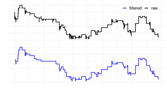
Figure 1: An example of a raw mid price and a filtered version with 0.1 seconds time interval

4.1 Basic result

The estimates were computed using the maximum likelihood method based on using the filtered data described in the previous subsection. The dynamics of the daily estimates of the filtered data from 2016 to 2019 are shown in Figures 2-5. An example of the estimates is also presented in B. Figure 2 shows the dynamics of $\mu_{1}$ and $\mu_{2}$ which are the daily estimated from the NVDA on the left. The overall trends of the two estimates are similar to each other, and on some days, are almost the same. However, there are also many days when the difference between $\mu_{1}$ and $\mu_{2}$ is significant, as in the right panel of the figure, where $\mu_{1}-\mu_{2}$ is plotted. Note that our formula of variances in the previous section does not exclude a case in which $\mu_{1}\neq\mu_{2}$.

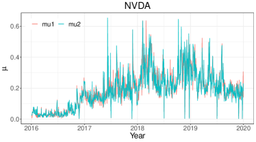
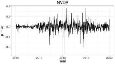
Figure 2: The dynamics of daily estimated $\mu$, NVDA from 2016 to 2019

There are four parameters in the $\bm{\alpha}$ matrix and the dynamics of daily estimates are plotted in Figure 3. On the left, we plot the dynamics of $\alpha_{1,1}$ and $\alpha_{2,2}$, which are also known as self-excitement parameters. On the right, we plot the dynamics of $\alpha_{1,2}$ and $\alpha_{2,1}$, which are also known as mutual excitement or cross-excitement parameters. In some studies, $\alpha_{1,1}=\alpha_{2,2}$ and $\alpha_{1,2}=\alpha_{2,1}$, that is the symmetric kernel matrix, is assumed to model parsimony. To some extent, the assumptions are reasonable due to the similar trends in each group. However, as in the case of $\mu$, we assume the general version of the excitement matrix $\bm{\alpha}$; that is no equality constraints for the elements of the matrix.

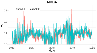
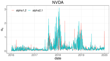
Figure 3: The dynamics of daily estimated $\alpha$, NVDA from 2016 to 2019

Figure 4 show the dynamics of $\beta_{1}$ and $\beta_{2}$ on the left. Similarly, with $\mu$, $\beta_{1}$ is similar to $\beta_{2}$; However, there are often days when $\beta_{1}$ and $\beta_{2}$ are significantly different. Therefore, we do not rule out the possibility that $\beta_{1}$ and $\beta_{2}$ are different.

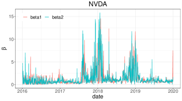
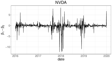
Figure 4: The dynamics of daily estimated $\beta$, NVDA from 2016 to 2019

Finally, Figure 5 shows the dynamics of the four parameters in $\bm{\eta}$. As in the case of $\bm{\alpha}$, $\eta_{1,1}$ is similar to $\eta_{2,2}$ and $\eta_{1,2}$ is similar to $\eta_{2,1}$. For simplicity, the assumption of the symmetric $\bm{\eta}$ matrix may be reasonable, especially when the small amount of data results in low statistical power. Since the data has sufficient observations, even for filtered ones, we did not assert any parameter constraint and estimate the volatility using the general model. For intraday estimations in the later, the amount of data to be used for estimations is relatively small, and the symmetric matrices for $\bm{\alpha}$ and $\bm{\eta}$ are assumed.

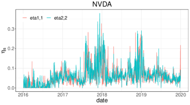
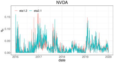
Figure 5: The dynamics of daily estimated $\eta$, NVDA from 2016 to 2019

We present quantile-quantile (Q-Q) plots of the residuals to check whether the model fits the filtered data well. Since the estimations are performed on a daily basis, one Q-Q plot can be generated for each day and stock. Examples of the Q-Q plots, the residuals versus the unit exponential distribution, are presented in Figure 6. Using the obtained estimates after estimation procedure, the fitted intensities, $\hat{\lambda}_{1}$ and $\hat{\lambda}_{2}$, are computed. Then, the residuals are computed by

$$\bigcup_{i=1,2}\left\{\int_{t_{i,j}}^{t_{i,j+1}}\hat{\lambda}_{i}(u)\mathrm{d}u\right\},$$

where $t_{i,j}$ denotes the corresponding event times.

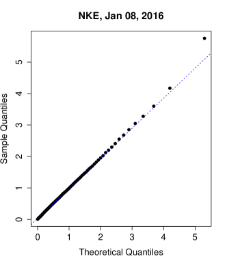
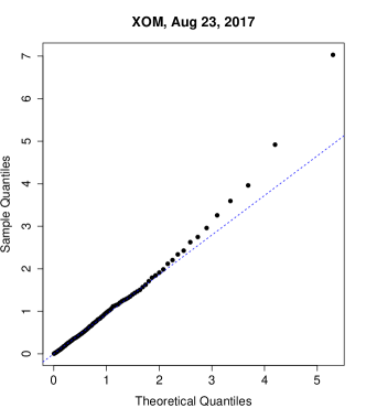
Figure 6: Q-Q plots of residuals

It is not possible to show the Q-Q plots of all the estimated data investigated; however, in general, we observe two types. First, the points of the Q-Q plot are very close to the straight line, indicating that the model fits the data very well. In this case, we cannot reject the null hypothesis that the distribution of the residual follows the unit exponential distribution. Second, the points of the Q-Q plot spread slightly above the straight line, and the estimated residuals have slightly thicker tails than the exponential distribution. In this case, the null hypothesis that the residual follows the exponential distribution is rejected at a typical significance level. However, we believe that it does not have a significant effect on the estimation of volatility.

4.2 Volatility dynamics

Using estimates and formulas in Section 3, the daily volatilities are measured. We show graphs to visually check whether the Hawkes volatility adequately measures stock price variability. Figure 7(a) shows the absolute daily price changes of NVDA stock from 2016 to 2019. Figure 7(c) shows the daily Hawkes volatilities computed under the assumption that the mark and intensities are independent, as in Corollary 14. In Figure 7(d), the daily Hawkes volatilities are calculated without excluding the possibility that the mark and intensities are dependent, as in Corollary 13. The overall trends of the two estimated volatilities are almost identical. It is a good way to assume independence between the marks and the underlying counting processes and intensities to simplify the procedure. The realized volatility, calculated following Andersen et al. (2003) as a benchmark, is also plotted in Figure 7(b). The three types of volatility show very similar dynamics. The time interval for computing the realized volatility was set to 5 minutes.

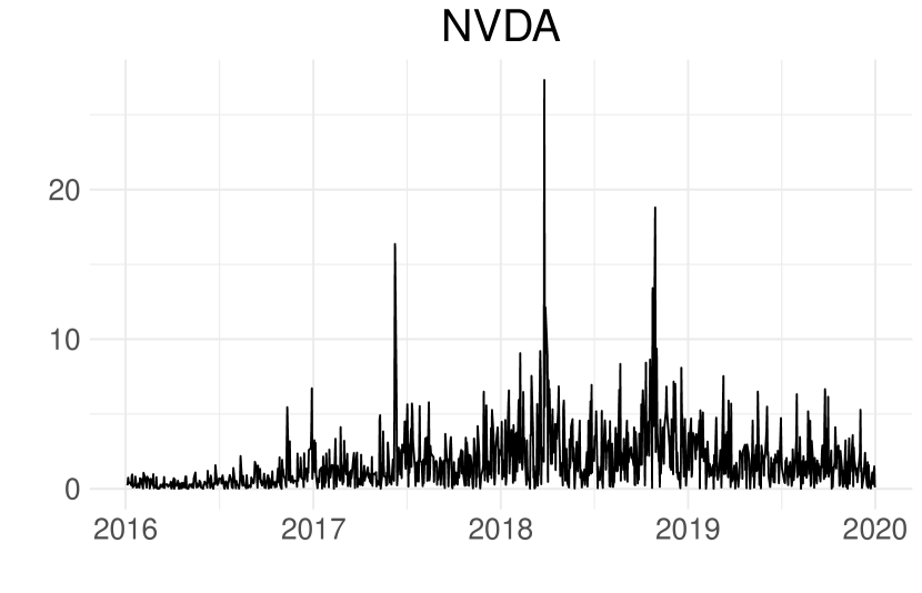
(a) Absolute daily price change

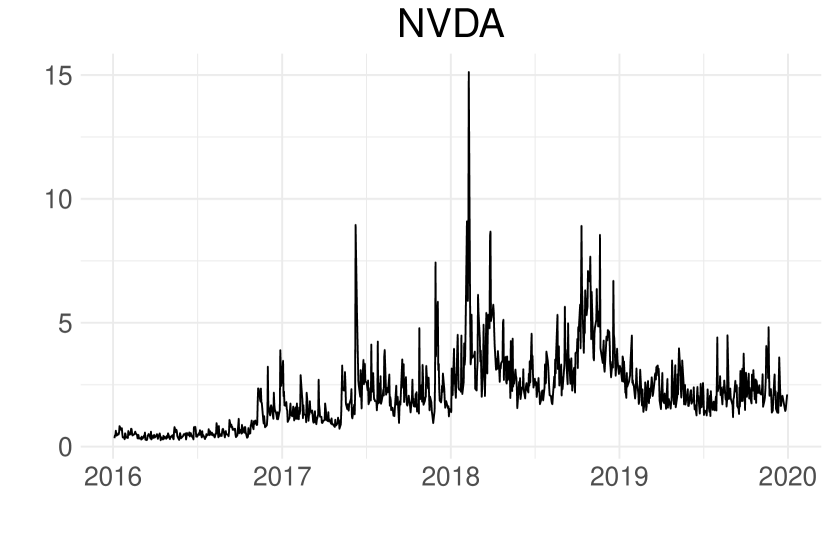
(b) Daily realized volatility

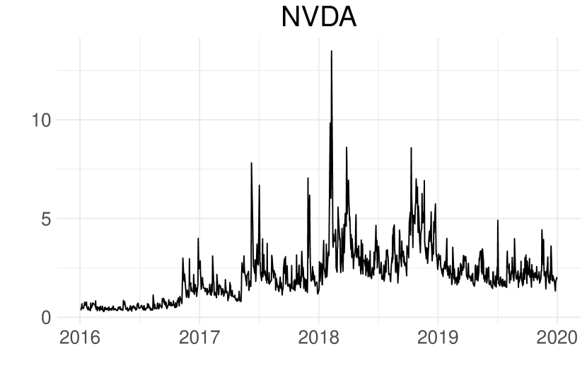
(c) Daily Hawkes volatility under independence

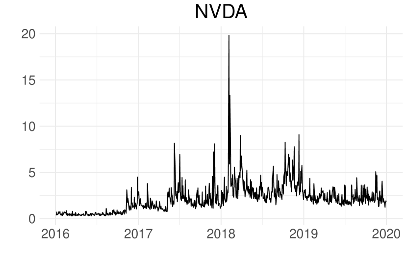
(d) Daily Hawkes volatility under dependence

Figure 7: Comparison of the dynamics of the daily estimated volatilities and the absolute price change

The backtesting method, which is often used in the Value-at-Risk analysis, was applied to test the performance of Hawkes volatility. It provides a graphical guideline for how well the volatility measure will perform. In Figure 8, the dynamics of the absolute daily price change from 2016 to 2017 are plotted with a black line. The two times of daily estimated Hawkes volatility, with the dependence assumption computed by Corollary 13, are plotted in a red line. Both lines have the same trend. In 2016, both the red and black lines had small values; in 2017, both lines had relatively large values. Judging from a graphical point of view, the Hawkes volatility seems to capture the variability in price change adequately.

The days in which the absolute daily price difference exceeded the two times of the Hawkes standard deviation are presented by blue circles. Although omitted in the figure, the total number of days in which the absolute price difference exceeded the two times of the Hawkes volatility were 50 days, which is around 5% of all observed days. Interestingly, this is consistent with the rule that approximately 95% of the data are within two standard deviations of the normal distribution. Further, the distribution of exceedances is spread uniformly over the entire period; that means the Hawkes model captures the volatility trend well.

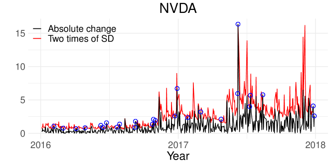
Figure 8: The exceeded absolute price change compared with two times of measured Hawkes volatility

Let us extend the discussion above to arbitrary multiples of standard deviation. Note that 68%, 95%, and 99.7% of the values lie within one, two, and three standard deviations in the mean zero normal distribution, respectively. In Figure 9, the x-axis denotes the number of multiples of the standard deviation. The y-axis is the proportion of price changes that do not exceed the corresponding multiples of the standard deviation. The blue line represents the Hawkes volatility, while the red line represents the probability that the data lies within the multiple of the standard deviation in the standard normal distribution. Interestingly, the two curves are almost identical. The Hawkes volatility is based on a model without excluding the possibility of dependence, but the volatility under the assumption of independence shows almost similar results. These results support Hawkes volatility as a reliable measure of price variability.

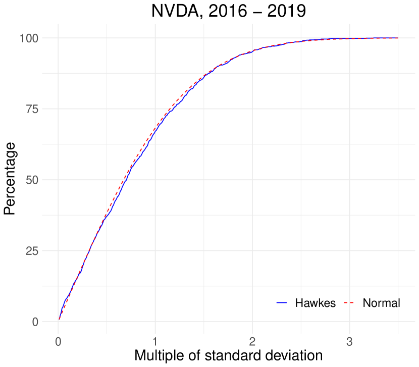
(a)

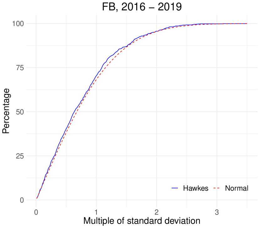
(b)

Figure 9: Percentage of absolute price change that lies with multiple of standard deviation

4.3 Intraday estimation

One of the important applications of the Hawkes volatility is that it can observe time-varying volatility in near real-time; that is, we can observe the dynamics of intraday volatility. This is due to the trading nature of the stock market, which provides the sufficient data for estimation, even in a short period of time. Under a 30-minute time window, the marked Hawkes model was adequately fitted and the volatility was calculated from the estimated parameters. For a small amount of data, we assume that $\bm{\alpha}$ and $\bm{\eta}$ are symmetric, to archive model parsimony. The time interval window for estimation is reset after 10 seconds.

In Figure 10, we plot the examples of the intraday volatilities from January 15, 2016 with a time line from 10:00 AM to 15:00 PM. On the left panel, it is interesting to note that volatility rebounds immediately after noon. It might represent the market participants returning to the stock market after lunch. The right panel more precisely shows the well-known U-shaped form of volatility. The real-time Hawkes volatility measure is expected to be useful for traders in managing intraday price risk. It allows them to observe market volatility for each stock in real time.

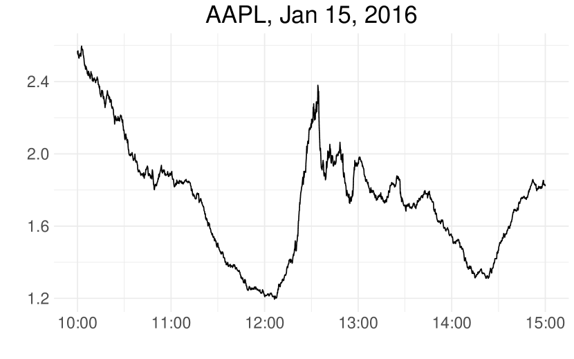
(a) AAPL

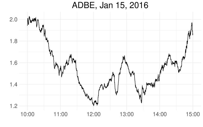
(b) ADBE

Figure 10: Intraday volatility dynamics in a typical day

Figure 11 shows another example in this regard, observed on Feb 20, 2020. On that day, the stock market, that had risen at the start as usual, suddenly declined from 10:45 AM for approximately one hour. Subsequently, it recovered gradually. Although the exact reason behind its decline is not known, it is suspected that the market had been highly volatile for a while, following the rapid spread of COVID-19. The Hawkes volatility illustrates the real-time volatility changes observed on this day in the figure, showing that the volatility rapidly increased until around 11:30 AM and then gradually stabilized.

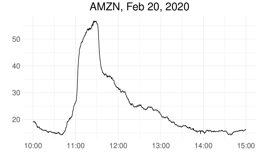
(a) AMZN

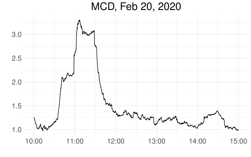
(b) MCD

Figure 11: Intraday volatility dynamics with sudden change in volatility

Typical volatility forecasting used in risk management is usually performed using a discrete time framework. Tomorrow’s volatility is predicted based on the historical return data up to today. The introduction of the intraday Hawkes volatility in this study and high-frequency data used, allow us to estimate volatility in near real-time throughout the day. We investigate whether the intraday volatility, which would be updated in real-time after the market opening, contains more information about the total real variation of the day’s return. Does the prediction, including updated intraday volatility, result in better than the volatility forecast calculated solely based on the return information up to the previous day? New information might be expected to bring better results for volatility prediction. If so, from when does the intraday volatility of the day contain more accurate information than the history up to the previous day? The Hawkes intraday volatility provides an answer to this question.

The opening and closing times of the stock market are expressed in discrete times, denoted by $t_{n}$ and $u_{n}$, respectively, for $1\leq n\leq N$. Then the daily return process is

$$R_{n}=\frac{S(u_{n})-S(t_{n})}{S(t_{n})}.$$

We first consider the GJR-GARCH model (Glosten et al., 1993) for a traditional volatility prediction under a discrete time setting. A simple variance model is used to simplify the test, but there will be no significant difference in the results even if the GARCH model with the mean is used. Under the model, the GARCH volatility at day $n$ is represented by

$$g^{2}_{n}=\omega_{g}+(\alpha_{g}+\gamma_{g}I_{\{R_{n-1}<0\}})\varepsilon_{n-1}^{2}+\beta_{g}g^{2}_{n-1}$$ (30)

with parameters $\omega_{g},\alpha_{g},\gamma_{g},\beta_{g}$ and $\varepsilon_{n}=R_{n}/g_{n}$. The estimates of the parameters, $\hat{\omega}_{g},\hat{\alpha}_{g},\hat{\gamma}_{g},\hat{\beta}_{g}$ are based on the maximum likelihood estimation with $m$ numbers of previous returns $R_{n-m},\cdots,R_{n-1}$. We use $m=1,500$ days for the empirical study. The one step ahead volatility prediction is accomplished by

$$\hat{g}^{2}_{n+1}=\hat{\omega}_{g}+(\hat{\alpha}_{g}+\hat{\gamma}_{g}I_{\{R_{n}<0\}})\varepsilon_{n}^{2}+\hat{\beta}_{g}\hat{g}^{2}_{n}.$$

This prediction is assumed to be computed before the opening of the stock market and can be used for daily risk management from a practical point of view.

After a risk manager predicts today’s volatility in advance, using a volatility model such as GARCH based on previous histories, the market now opens and new tick information begins to flow in. With this new influx of information, the manager starts to estimate today’s Hawks volatility in real-time. Let $\hat{h}_{n}(T)$ be the estimated Hawkes volatility defined by Corollary 13 based on data from the opening time $t_{n}$ to $t_{n}+T\leq u_{n}$ under the symmetric kernel. We now establish a simple linearly combined volatility measure:

$$\sigma_{n}(T)=\theta_{1}(T)g_{n}+\theta_{2}(T)h_{n}(T)$$ (31)

The above equation is establish to determine whether the volatility measurement performance is improved when intraday Hawkes volatility up to time $t_{n}+T$ is added to the traditional GARCH volatility measure. When applied to actual empirical studies, the estimates of $g_{n}$ and $h_{n}$ are used:

$$\hat{\sigma}_{n}(T)=\theta_{1}(T)\hat{g}_{n}+\theta_{2}(T)\hat{h}_{n}(T).$$

More specifically, $\sigma_{n}(T)$ is the $n$-day volatility, a linear combination of the predicted GARCH volatility based on the past $m$-return data and the Hawkes volatility measured from the opening time $t_{n}$ to $t_{n}+T$.

Next, we estimate $\theta_{1}(T)$ and $\theta_{2}(T)$ using $\hat{g}_{n}$ and $\hat{\theta}_{n}$, for $1\leq n\leq N$. Note that the parameters in Eq. (30) are newly estimated as $n$ changes. With fixed $T$, we find $\hat{\theta}(T)$s such that

$$\hat{\theta}_{1}(T),\hat{\theta}_{2}(T)=\mathrm{argmax}_{\theta_{1},\theta_{2}}\ell_{T}(R_{1},\cdots,R_{N};\hat{\sigma}_{1}(T),\cdots,\hat{\sigma}_{N}(T))$$ (32)

where $\ell_{T}$ is the log-likelihood function of $N$ independent mean-zero multivariate normal variables with a vector of standard deviations $\hat{\sigma}_{1}(T),\cdots,\hat{\sigma}_{N}(T)$.

Using data from AAPL, 2016-2019, the GARCH model was estimated with daily return time series data, and intraday data were used to compute intraday Hawks volatility. As seen in the left of Figure 12, the log-likelihood $\ell_{T}$ in Eq. (32) increases monotonically as time $T$ goes after the market opening. This implies that the influx of new information regarding intraday price changes makes daily volatility predictions more accurate. Intraday changes in $\theta(T)$s over time $T$ are compared in the right of Figure 12. In the early stage of the market, $\theta_{1}$ of GARCH is larger than $\theta_{2}$; that is, the GARCH volatility predicted before the market opening has more predicting power than the intraday Hawkes volatility. However the $\theta_{2}$ of the Hawkes volatility dominates in the role of volatility prediction after around 10:00 AM. About $T=30$ minutes after the market opens, the information from $t_{n}$ to $t_{n}+T$ for predicting daily volatility is very rich, and the role of volatility information of the past days is rapidly reduced.

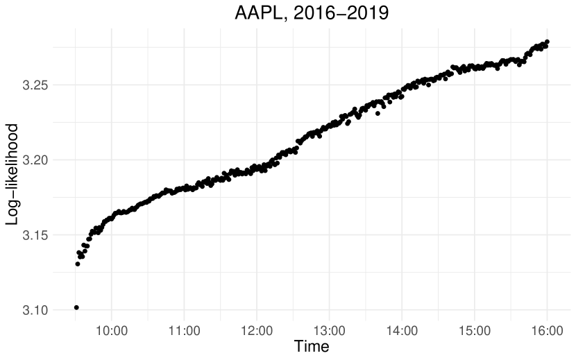
(a) Log-likelihood

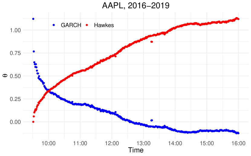
(b) $\theta$

Figure 12: The predictive power of Hawkes volatility growing stronger over time during a day

4.4 Futures and stock volatility

This subsection examines the relationship between the pre-market volatility of E-Mini S&P 500 futures and stock price volatility during the regular market session. The regular stock market opens from 9:30 a.m. to 4 p.m; however, E-Mini S&P 500 futures trade from 6:00 p.m. to 5:00 p.m. of the following day. E-mini S&P 500 futures are almost continuously traded even when stocks are not traded in regular exchanges, and the Hawkes volatility of E-Mini futures can be estimated using data from this period of non-regular market session. This study investigates how much the volatility of E-Mini S&P 500 futures, observed before the market opening (non-regular trading time), has the explanatory power to stock market volatility after market opening.

As in the previous subsection, let $\hat{h}^{s}_{n}(T_{1})$ be the estimated intraday Hawkes volatility defined by Corollary 13 based on stock prices observed from the opening time, $t_{n}$, to $t_{n}+T_{1}$ of $n$-th day, where $t_{n}+T_{1}$ is a time between the open and close of the regular trading session. In addition, let $\hat{h}^{f}_{n}(T_{2})$ be the estimated Hawkes volatility based on E-Mini S&P 500 futures mid-price process from $t_{n}-T_{2}$ to the opening time $t_{n}$; that is, before the regular trading time where $T_{2}$ is set to be not to cross over the halting time of trades, 6:00 p.m. Then, we establish a linear model such that

$$\hat{h}^{s}_{n}(T_{1})=\beta_{0}+\beta_{1}\hat{h}^{f}_{n}(T_{2})+\epsilon_{n},$$ (33)

which examines the relationship between the stock volatility $\hat{h}^{s}_{n}(T_{1})$ after market opening and the futures volatility $\hat{h}^{f}_{n}(T_{2})$ before the market opening. If there is more than one futures price data available on a specific date, the volatility of futures with closer expiration date is used.

Since the regression analysis in Eq. (33) can be performed on any $0<T_{1}\leq 6.5\textrm{ hours}$ and $0<T_{2}\leq 16.5\textrm{ hours}$, the adjusted R-squared, $R^{2}(T_{1},T_{2})$, of the linear model is considered as a function of $T_{1}$ and $T_{2}$. By examining available $T_{1}$ and $T_{2}$, we can get the overall shape of R-squared. Its empirical result is presented in Figure 13 which presents R-squared surface as a function of $T_{1}$ and $T_{2}$, where AAPL’s intraday price process is used for stock volatility, which accounts for approximately 7% of the S&P 500 index. Data for stock and futures for the estimation of the linear model are for 2019.

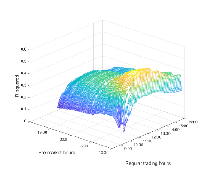
Figure 13: The adjusted R-squared that explain the relationship between the pre-market volatility of E-Mini S&P 500 futures and stock price volatility during the regular trading time

According to the figure, the best pre-market predictor in terms of R-squared of the Hawkes volatility of AAPL based on E-mini data is Emini’s volatility calculated by the information accumulated from approximately 7-8 AM to the market opening time 9:30 AM. As a target variable, the AAPL intraday volatilities are best predicted based on the period from market open to around noon. More precisely, in this example, the best predictor is the pre-market E-mini Hawkes volatility estimated at the interval of 7:45 AM to 9:30 AM, and the best-predicted period of AAPL intraday volatility is from 9:30 AM to 11:30 AM with the adjusted R-squared of 0.52. In summary, the explanatory power of pre-market futures volatility to AAPL volatility increases little by little after the market opens, peaks around 11:30, and gradually decreases over time.

4.5 Forecasting

In the previous section, the empirical study shows that the market futures volatility explains the regular trading time stock volatility well. In this section, we examine whether pre-market futures volatility can improve more stock volatility forecasting than the forecasting solely based on previous stock market data in terms of the Hawkes volatility.

First, if there is no information on pre-market futures volatility and the information of the Hawkes daily volatility of stock is only available, the following traditional AR(2) model on daily Hawkes volatilities can be considered:

$$h^{s}_{n}=\phi_{0}+\phi_{1}h^{s}_{n-1}+\phi_{2}h^{s}_{n-2}+\epsilon_{n}$$ (34)

where $h^{s}_{n}$ is the daily Hawkes volatility on $n$-th day. Among various linear time series models, the AR(2) model is selected by Hyndman and Khandakar (2008) algorithm.

More precisely, the daily Hawkes volatility estimation based on tick data for each day is preceded as demonstrated in Figure 7. Thus, before $n$-th day, we have $M$ numbers of estimated daily Hawkes volatilities $\hat{h}^{s}_{i}$, for $n-M+1\leq i\leq n$. The estimated Hawkes volatilities are used to fit the linear model in Eq. (34) and find the estimates of $\phi_{0},\phi_{1}$ and $\phi_{2}$. Of course these estimates are updated as each day passes and new data is introduced. The one-step ahead forecasting of the Hawkes volatility for the day of $n+1$ at $n$-th day is

$$\check{h}^{s}_{n+1}=\hat{\phi}_{0}+\hat{\phi}_{1}\hat{h}^{s}_{n}+\hat{\phi}_{2}\hat{h}^{s}_{n-1}(T).$$

Second, consider the following model, including pre-market futures volatility as a predictor variable:

$$h^{s}_{n}=\psi_{0}+\psi_{1}h^{s}_{n-1}+\psi_{2}h^{s}_{n-2}+\psi_{3}h^{f}_{n}(T)+\varepsilon_{n}$$ (35)

where $h^{f}_{n}(T)$ denotes the pre-market futures Hawkes volatility with the length of time interval, $T$, measured right before the market open; that is, from $t_{n}-T$ to $t_{n}$. Compared with Eq. (34), the term $h^{s}_{n-2}$ is removed. By introducing $h^{f}_{n}(T)$, $h^{s}_{n-2}$ is not significant anymore according to our empirical study. Similar to before, the daily Hawkes volatility estimations for the futures and stock are preceded. After that the model in Eq. (35) is fitted to find $\hat{\psi}_{0},\hat{\psi}_{1}$ and $\hat{\psi}_{1}$ based on the volatilities estimated before the $n$-th day. The Hawkes volatility of stock at $(n+1)$-day is forecasted by

$$\tilde{h}_{n+1}(T)=\hat{\psi}_{0}+\hat{\psi}_{1}\hat{h}^{s}_{n}+\hat{\psi}_{2}\hat{h}^{f}_{n+1}(T).$$

For both cases, the root mean square relative errors are defined. For Eq. (34), we have

$$\mathrm{RMSRE}_{s}=\sqrt{\frac{1}{N}\sum_{n=1}^{N}\left(\frac{\check{h}^{s}_{n+1}-\hat{h}^{s}_{n+1}}{\check{h}^{s}_{n+1}}\right)^{2}}$$

and for Eq. (35), we have

$$\mathrm{RMSRE}_{f}(T)=\sqrt{\frac{1}{N}\sum_{n=1}^{N}\left(\frac{\tilde{h}^{s}_{n+1}(T)-\hat{h}^{s}_{n+1}}{\tilde{h}^{s}_{n+1}(T)}\right)^{2}}.$$

Note that $\check{h}^{s}$ and $\tilde{h}^{s}$ are different from $\hat{h}^{s}$ such that $\check{h}^{s}_{n}$ and $\tilde{h}^{s}_{n}$ are computed and forecasted based on past data but $\hat{h}^{s}_{n}$ is estimated by the tick data of $n$-th day.

Empirical results show a smaller error when forecasting was carried out through the model including the pre-market futures volatility. Figure 14 shows that the prediction with futures volatility as a predictor variable improve the RMSRE using any pre-market time interval $[t_{n}-T,t_{n}]$ where $t_{n}-T$ is represented by the values on the $x$-axis. In the figure, the dots present $\mathrm{RMSRE}_{f}(T)$ and the solid line is the $\mathrm{RMSRE}_{s}$, which does depend on $T$. The data used for forecasting ranges from 2018 to 2019 and the training for each linear model at $n$-th day uses previous 400 data and includes from 2016. The figure also shows that the pre-market futures volatility, measured right before the market opening, reduces the error more.

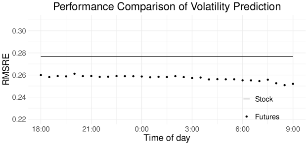
Figure 14: Comparison between $\mathrm{RMSRE}_{s}$ (solid line) and $\mathrm{RMSRE}_{f}(T)$ (dotted line)

5 Conclusion

In this study, the up and down movements of price dynamics at the tick level are modeled by the self and mutually exciting Hawkes processes. The variance formulas of the difference between the number of ups and downs are derived in both the non-marked and marked models. Under the marked Hawkes model, the formula is presented for both the dependent and independent mark distributions, considering the underlying intensity and counting processes. The variance formula is applied to the filtered high-frequency data observed by every 0.1 second; the single kernel Hawkes models fit well to this data.

Through a comparison with realized volatility, we confirm that the Hawkes model adequately measures daily volatility. The biggest advantage of Hawkes volatility is intraday volatility, which allows the precise measurement of real-time instantaneous variability in price. Intraday Hawkes volatility has a stronger predictive power for daily volatility, which increases with time. According to our findings, the importance of intraday Hawkes volatility around 10 o’clock in the stock market outweighs GARCH volatility, a discrete-time volatility prediction model depending on a time series of daily returns up to the last day. The Hawkes intraday volatility makes it possible to precisely examine the predictive power of the volatility in the futures market, before the stock market opening, to the stock price volatility after market opening. In addition, using the volatility of the pre-market futures as well as the volatility of stocks has an improvement in stock market volatility forecasting.

Appendix A Proofs

Proof of Proposition 1.

By taking expectations on both sides of Eq. (4),

$$\mathbb{E}[\bm{\lambda}_{t}] =\mathbb{E}[\bm{\lambda}_{0}]+\int_{0}^{t}\{\bm{\beta}\bm{\mu}+(\bm{\alpha}-\bm{\beta})\mathbb{E}[\bm{\lambda}_{s}])\}\mathrm{d}s$$

$$=\mathbb{E}[\bm{\lambda}_{t}]+\{\bm{\beta}\bm{\mu}+(\bm{\alpha}-\bm{\beta})\mathbb{E}[\bm{\lambda}_{t}])\}t,$$

where we use $\mathbb{E}[\bm{\lambda}_{t}]=\mathbb{E}[\bm{\lambda}_{s}]=\mathbb{E}[\bm{\lambda}_{0}]$ to obtain Eq. (5). ∎

Proof of Proposition 3.

By Lemma 2,

$$\mathrm{d}(\bm{\lambda}_{t}\bm{\lambda}_{t}^{\top})={} \bm{\lambda}_{t}\mathrm{d}\bm{\lambda}_{t}^{\top}+\mathrm{d}(\bm{\lambda}_{t})\bm{\lambda}^{\top}_{t}+\mathrm{d}[\bm{\lambda},\bm{\lambda}^{\top}]_{t}$$

$$={} \left[\bm{\lambda}_{t}\{\bm{\beta}\bm{\mu}+(\bm{\alpha}-\bm{\beta})\bm{\lambda}_{t}\}^{\top}+\{\bm{\beta}\bm{\mu}+(\bm{\alpha}-\bm{\beta})\bm{\lambda}_{t}\}\bm{\lambda}_{t}^{\top}\right]\mathrm{d}t+\bm{\alpha}\mathrm{Dg}(\mathrm{d}\bm{N}_{t})\bm{\alpha}^{\top}$$

$$+\bm{\lambda}_{t}\{\bm{\alpha}(\mathrm{d}\bm{N}_{t}-\bm{\lambda}_{t}\mathrm{d}t)\}^{\top}+\bm{\alpha}(\mathrm{d}\bm{N}_{t}-\bm{\lambda}_{t}\mathrm{d}t)\bm{\lambda}_{t}^{\top}$$

By taking expectation in an integration form,

$$\mathbb{E}[\bm{\lambda}_{t}\bm{\lambda}_{t}^{\top}]=\mathbb{E}[\bm{\lambda}_{0}\bm{\lambda}_{0}^{\top}]+\int_{0}^{t} \left\{\mathbb{E}[\bm{\lambda}_{s}\bm{\lambda}_{s}^{\top}](\bm{\alpha}-\bm{\beta})^{\top}+(\bm{\alpha}-\bm{\beta})\mathbb{E}[\bm{\lambda}_{s}\bm{\lambda}_{s}^{\top}]\right.$$

$$\left.+\mathbb{E}[\bm{\lambda}_{s}](\bm{\beta}\bm{\mu})^{\top}+\bm{\beta}\bm{\mu}\mathbb{E}[\bm{\lambda}_{s}^{\top}]+\bm{\alpha}\mathrm{Dg}(\mathbb{E}[\bm{\lambda}_{s}])\bm{\alpha}^{\top}\right\}\mathrm{d}s.$$

By using $\mathbb{E}[\bm{\lambda}_{t}\bm{\lambda}_{t}^{\top}]=\mathbb{E}[\bm{\lambda}_{s}\bm{\lambda}_{s}^{\top}]=\mathbb{E}[\bm{\lambda}_{0}\bm{\lambda}_{0}^{\top}]$, the integrand should be zero, and we have the desired result. ∎

Proof of Proposition 4.

By Lemma 2,

$$\mathrm{d}(\bm{\lambda}_{t}\bm{N}_{t}^{\top}) =\bm{\lambda}_{t}\mathrm{d}\bm{N}_{t}^{\top}+\mathrm{d}(\bm{\lambda}_{t})\bm{N}^{\top}_{t-}+\mathrm{d}[\bm{\lambda}\bm{N}^{\top}]_{t}$$

$$=\bm{\lambda}_{t}\mathrm{d}\bm{N}_{t}^{\top}+\{\bm{\beta}(\bm{\mu}-\bm{\lambda}_{t})\mathrm{d}t+\bm{\alpha}\mathrm{d}\bm{N}_{t}\}\bm{N}^{\top}_{t-}+\bm{\alpha}\mathrm{Dg}(\mathrm{d}\bm{N}_{t})$$

and

$$\mathbb{E}[\bm{\lambda}_{t}\bm{N}^{\top}_{t}]=\int_{0}^{t}\left\{\mathbb{E}[\bm{\lambda}_{s}\bm{\lambda}^{\top}_{s}]+\bm{\beta}\bm{\mu}\mathbb{E}[\bm{\lambda}_{s}^{\top}]s+(\bm{\alpha}-\bm{\beta})\mathbb{E}[\bm{\lambda}_{s}\bm{N}_{s}^{\top}]+\bm{\alpha}\mathrm{Dg}(\mathbb{E}[\bm{\lambda}_{s}])\right\}\mathrm{d}s$$

or as a system of linear differential equation,

$$\frac{\mathrm{d}\mathbb{E}[\bm{\lambda}_{t}\bm{N}_{t}^{\top}]}{\mathrm{d}t}=(\bm{\alpha}-\bm{\beta})\mathbb{E}[\bm{\lambda}_{t}\bm{N}_{t}^{\top}]+\bm{\beta}\bm{\mu}\mathbb{E}[\bm{\lambda}_{t}^{\top}]t+\mathbb{E}[\bm{\lambda}_{t}\bm{\lambda}_{t}^{\top}]+\bm{\alpha}\mathrm{Dg}(\mathbb{E}[\bm{\lambda}_{t}]).$$

∎

Proof of Theorem 5.

Let $f(x_{1},x_{2})=(x_{1}-x_{2})^{2}$. The infinitesimal generator on $N_{1}(t)$ and $N_{2}(t)$ defined by its action on $f(N_{1}(t),N_{2}(t))$ is

$$\mathcal{A}f(N_{1}(t),N_{2}(t))={} \lim_{h\downarrow 0}\frac{\mathbb{E}[f(N_{1}(t+h),N_{2}(t+h))-f(N_{1}(t),N_{2}(t))|\mathcal{F}_{t}]}{h}$$

$$={} \lambda_{1}(t)\{f(N_{1}(t)+1,N_{2}(t))-f(N_{1}(t),N_{2}(t)\}$$

$$+\lambda_{2}(t)\{f(N_{1}(t),N_{2}(t)+1)-f(N_{1}(t),N_{2}(t))\}$$

$$={} \lambda_{1}(t)\{2N_{1}(t)-2N_{2}(t)+1)\}+\lambda_{2}(t)\{2N_{2}(t)-2N_{1}(t)+1\}.$$

By Dynkin’s formula,

$$\mathbb{E}\left[(N_{1}(t)-N_{2}(t))^{2}\right]=\int_{0}^{t}\mathbb{E}[\mathcal{A}f(N_{1}(s),N_{2}(s))]\mathrm{d}s$$

$$={} \int_{0}^{t}\mathbb{E}\left[\lambda_{1}(s)\{2N_{1}(s)-2N_{2}(s)+1)\}+\lambda_{2}(s)\{2N_{2}(s)-2N_{1}(s)+1\}\right]\mathrm{d}s$$

$$={} \int_{0}^{t}\left\{2\begin{bmatrix}1&-1\end{bmatrix}\mathbb{E}[\bm{\lambda}_{s}\bm{N}_{s}^{\top}]\begin{bmatrix}1\\ -1\end{bmatrix}+\begin{bmatrix}1&1\end{bmatrix}\mathbb{E}[\bm{\lambda}_{s}]\right\}\mathrm{d}s$$

$$={} \int_{0}^{t}\left\{2\begin{bmatrix}1&-1\end{bmatrix}\left(\bm{\mathrm{V}}\bm{\mathrm{C}}\circ\begin{bmatrix}\mathrm{e}^{\xi_{1}s}&\mathrm{e}^{\xi_{1}s}\\ \mathrm{e}^{\xi_{2}s}&\mathrm{e}^{\xi_{2}s}\end{bmatrix}+\bm{\mathrm{A}}s+\bm{\mathrm{B}}\right)\begin{bmatrix}1\\ -1\end{bmatrix}+\begin{bmatrix}1&1\end{bmatrix}\mathbb{E}[\bm{\lambda}_{s}]\right\}\mathrm{d}s$$

$$={} 2\begin{bmatrix}1&-1\end{bmatrix}\left(\bm{\mathrm{V}}\bm{\mathrm{D}}\circ\begin{bmatrix}\mathrm{e}^{\xi_{1}t}-1&\mathrm{e}^{\xi_{1}t}-1\\ \mathrm{e}^{\xi_{2}t}-1&\mathrm{e}^{\xi_{2}t}-1\end{bmatrix}+\frac{1}{2}\bm{\mathrm{A}}t^{2}+\bm{\mathrm{B}}t\right)\begin{bmatrix}1\\ -1\end{bmatrix}+\begin{bmatrix}1&1\end{bmatrix}\mathbb{E}[\bm{\lambda}_{t}]t$$

where

$$\bm{\mathrm{D}}=\bm{\mathrm{C}}\circ\begin{bmatrix}\xi_{1}^{-1}&\xi_{1}^{-1}\\ \xi_{2}^{-1}&\xi_{2}^{-1}\end{bmatrix}.$$

Finally, the variance formula is derived by using

$$\mathbb{E}[(N_{1}(t)-N_{2}(t))]^{2}=\begin{bmatrix}1&-1\end{bmatrix}\mathbb{E}[\bm{\lambda}_{s}]\mathbb{E}[\bm{\lambda}_{s}]^{\top}\begin{bmatrix}1\\ -1\end{bmatrix}t^{2}=\begin{bmatrix}1&-1\end{bmatrix}\bm{\mathrm{A}}\begin{bmatrix}1\\ -1\end{bmatrix}t^{2}$$

and

$$\mathrm{Var}(N_{1}(t)-N_{2}(t))=\mathbb{E}[(N_{1}(t)-N_{2}(t))]^{2}-(\mathbb{E}[N_{1}(t)-N_{2}(t)])^{2}.$$

∎

Proof for Propositon 6.

Since

$$\mathbb{E}\left[\mathbb{K}_{t}[\bm{g}(z)]\bm{\lambda}_{t}\right]=\bm{\eta}\circ(\overline{\bm{\mathrm{Z}}}-1)\mathbb{E}[\bm{\lambda}_{t}],$$

we have

$$\mathbb{E}[\bm{\lambda}_{t}] =\mathbb{E}[\bm{\lambda}_{t}]+\{\bm{\beta}\bm{\mu}+(\bm{\alpha}+\bm{\eta}\circ(\overline{\bm{\mathrm{Z}}}-1)-\bm{\beta})\mathbb{E}[\bm{\lambda}_{t}]\}t.$$

Using $\mathbb{E}[\bm{\lambda}_{t}]=\mathbb{E}[\bm{\lambda}_{s}]=\mathbb{E}[\bm{\lambda}_{0}]$, we obtain Eq. (17). ∎

Proof for Lemma 8.

Since these expressions are the results of simple matrix calculations, only some parts of the proofs are briefly explained. For Eq. (19), since

$$\bm{g}(z)\mathrm{Dg}(\bm{M}(\mathrm{d}s\times\mathrm{d}z))\bm{g}(z)^{\top}={} (\bm{\alpha}-\bm{\eta}+\bm{\eta}\circ\bm{\mathrm{Z}})\mathrm{Dg}(\bm{M}(\mathrm{d}s\times\mathrm{d}z))(\bm{\alpha}-\bm{\eta}+\bm{\eta}\circ\bm{\mathrm{Z}})^{\top}$$

$$={} (\bm{\alpha}-\bm{\eta}+\bm{\eta}\circ\bm{\mathrm{Z}})\mathrm{Dg}(\bm{M}(\mathrm{d}s\times\mathrm{d}z))(\bm{\alpha}-\bm{\eta})^{\top}$$

$$+(\bm{\alpha}-\bm{\eta})\mathrm{Dg}(\bm{M}(\mathrm{d}s\times\mathrm{d}z))(\bm{\eta}\circ\bm{\mathrm{Z}})^{\top}$$

$$+(\bm{\eta}\circ\bm{\mathrm{Z}})\mathrm{Dg}(\bm{M}(\mathrm{d}s\times\mathrm{d}z))(\bm{\eta}\circ\bm{\mathrm{Z}})^{\top}$$

and

$$\begin{aligned} &\mathbb{E}\left[\int_{(0,t]\times E}(\bm{\eta}\circ\bm{\mathrm{Z}})\mathrm{Dg}(\bm{M}(\mathrm{d}s\times\mathrm{d}z))(\bm{\eta}\circ\bm{\mathrm{Z}})^{\top}\right]\\ &=\int_{(0,t]\times E}\left[\begin{matrix}\eta_{11}^{2}\mathbb{E}[z_{1}^{2}M_{1}(\mathrm{d}s\times\mathrm{d}z_{1})]+\eta_{12}^{2}\mathbb{E}[z_{2}^{2}M_{2}(\mathrm{d}s\times\mathrm{d}z_{2})]\\ \eta_{11}\eta_{21}\mathbb{E}[z_{1}^{2}M_{1}(\mathrm{d}s\times\mathrm{d}z_{1})]+\eta_{12}\eta_{22}\mathbb{E}[z_{2}^{2}M_{2}(\mathrm{d}s\times\mathrm{d}z_{2})]\end{matrix}\right.\\ &\qquad\qquad\qquad\qquad\qquad\qquad\qquad\qquad\left.\begin{matrix}\eta_{11}\eta_{21}\mathbb{E}[z_{1}^{2}M_{1}(\mathrm{d}s\times\mathrm{d}z_{1})]+\eta_{12}\eta_{22}\mathbb{E}[z_{2}^{2}M_{2}(\mathrm{d}s\times\mathrm{d}z_{2})]\\ \eta_{21}^{2}\mathbb{E}[z_{1}^{2}M_{1}(\mathrm{d}s\times\mathrm{d}z_{1})]+\eta_{22}^{2}\mathbb{E}[z_{2}^{2}M_{2}(\mathrm{d}s\times\mathrm{d}z_{2})]\end{matrix}\right]\mathrm{d}s\\ &=\int_{(0,t]\times E}\left[\begin{matrix}\eta_{11}^{2}Z^{(2)}_{1}\mathbb{E}[\lambda_{1}(s)]+\eta_{12}^{2}Z^{(2)}_{2}\mathbb{E}[\lambda_{2}(s)]\\ \eta_{11}\eta_{21}Z^{(2)}_{1}\mathbb{E}[\lambda_{1}(s)]+\eta_{12}\eta_{22}Z^{(2)}_{2}\mathbb{E}[\lambda_{2}(s)]\end{matrix}\right.\\ &\qquad\qquad\qquad\qquad\qquad\qquad\qquad\qquad\qquad\qquad\quad\left.\begin{matrix}\eta_{11}\eta_{21}Z^{(2)}_{1}\mathbb{E}[\lambda_{1}(s)]+\eta_{12}\eta_{22}Z^{(2)}_{2}\mathbb{E}[\lambda_{2}(s)]\\ \eta_{21}^{2}Z^{(2)}_{1}\mathbb{E}[\lambda_{1}(s)]+\eta_{22}^{2}Z^{(2)}_{2}\mathbb{E}[\lambda_{2}(s)]\end{matrix}\right]\mathrm{d}s\\ &=\int_{0}^{t}\left(\bm{\eta}\circ\bm{\mathrm{Z}}^{(2)\circ\frac{1}{2}}\right)\mathrm{Dg}(\mathbb{E}[\bm{\lambda}_{s}])\left(\bm{\eta}\circ\bm{\mathrm{Z}}^{(2)\circ\frac{1}{2}}\right)^{\top}\mathrm{d}s\end{aligned}$$

we have the desired result. For Eq. (20),

$$(\bm{\alpha}+\bm{g}(z))\mathrm{Dg}(\bm{M}(\mathrm{d}s\times\mathrm{d}z))\mathrm{Dg}(z)\\ =(\bm{\alpha}-\bm{\eta})\mathrm{Dg}(\bm{M}(\mathrm{d}s\times\mathrm{d}z))\mathrm{Dg}(z)+(\bm{\eta}\circ\bm{\mathrm{Z}})\mathrm{Dg}(\bm{M}(\mathrm{d}s\times\mathrm{d}z))\mathrm{Dg}(z)$$

and

$$\mathbb{E}\left[\int_{(0,t]\times E}(\bm{\alpha}-\bm{\eta})\mathrm{Dg}(\bm{M}(\mathrm{d}s\times\mathrm{d}z))\mathrm{Dg}(z)\right]$$

$$=\int_{(0,t]\times E}\mathbb{E}\left[\begin{matrix}(\alpha_{11}-\eta_{11})z_{1}M_{1}(\mathrm{d}s\times\mathrm{d}z_{1})&(\alpha_{12}-\eta_{12})z_{2}M_{2}(\mathrm{d}s\times\mathrm{d}z_{2})\\ (\alpha_{21}-\eta_{21})z_{1}M_{1}(\mathrm{d}s\times\mathrm{d}z_{1})&(\alpha_{22}-\eta_{22})z_{2}M_{2}(\mathrm{d}s\times\mathrm{d}z_{2})\end{matrix}\right]\mathrm{d}s$$

$$=(\bm{\alpha}-\bm{\eta})\circ\overline{\bm{\mathrm{Z}}}\mathrm{Dg}(\mathbb{E}[\bm{\lambda}_{t}])t.$$

Similarly,

$$\mathbb{E}\left[\int_{(0,t]\times E}(\bm{\eta}\circ\bm{\mathrm{Z}})\mathrm{Dg}(\bm{M}(\mathrm{d}s\times\mathrm{d}z))\mathrm{Dg}(z)\right] =\mathbb{E}\left[\int_{(0,t]\times E}(\bm{\eta}\circ\bm{\mathrm{Z}}^{\circ 2})\mathrm{Dg}(\bm{M}(\mathrm{d}s\times\mathrm{d}z))\right]$$

$$=\bm{\eta}\circ\overline{\bm{\mathrm{Z}}}^{(2)}\mathrm{Dg}(\mathbb{E}[\bm{\lambda}_{t}])t.$$

∎

Proof for Lemma 9.

Use

$$\bm{X}_{t}\bm{Y}^{\top}_{t} =\bm{X}_{0}\bm{Y}^{\top}_{0}+\int_{0}^{t}\bm{X}_{s-}\mathrm{d}\bm{Y}^{\top}_{s}+\int_{0}^{t}\mathrm{d}(\bm{X}_{s})\bm{Y}^{\top}_{s-}+[\bm{X}\bm{Y}^{\top}]_{t}$$

where

$$\int_{0}^{t}\bm{X}_{s-}\mathrm{d}\bm{Y}^{\top}_{u} =\int_{0}^{t}\bm{X}_{s}\bm{b}_{s}^{\top}\mathrm{d}s+\int_{(0,t]\times E}\bm{X}_{s-}\bm{M}^{\top}(\mathrm{d}s\times\mathrm{d}z)\bm{f}_{y}(s,z)^{\top}$$

$$\int_{0}^{t}\mathrm{d}(\bm{X}_{s})\bm{Y}^{\top}_{s-} =\int_{0}^{t}\bm{a}_{s}\bm{Y}_{s}^{\top}\mathrm{d}s+\int_{(0,t]\times E}\bm{f}_{x}(s,z)\bm{M}(\mathrm{d}s\times\mathrm{d}z)\bm{Y}_{s-}^{\top}$$

$$[\bm{X}\bm{Y}^{\top}]_{t} =\int_{(0,t]\times E}\bm{f}_{x}(s,z)\mathrm{Dg}(\bm{M}(\mathrm{d}s\times\mathrm{d}z))\bm{f}_{y}(s,z)^{\top}$$

and

$$\mathbb{E}\left[\int_{(0,t]\times E}\bm{X}_{s-}\bm{M}^{\top}(\mathrm{d}s\times\mathrm{d}z)\bm{f}_{y}(s,z)^{\top}\right]=\int_{0}^{t}\mathbb{E}\left[\bm{X}_{s}\bm{\lambda}_{s}^{\top}\mathbb{K}_{s}[\bm{f}_{y}(s,z)]^{\top}\right]\mathrm{d}s$$

$$\mathbb{E}\left[\int_{(0,t]\times E}\bm{f}_{x}(s,z)\bm{M}(\mathrm{d}s\times\mathrm{d}z)\bm{Y}_{s-}^{\top}\right]=\int_{0}^{t}\mathbb{E}\left[\mathbb{K}_{s}[\bm{f}_{x}(s,z)]\bm{\lambda}_{s}\bm{Y}^{\top}_{s}\right]\mathrm{d}s.$$

∎

Proof for Propositoin 10.

Since the intensity matrix process follows Eq. (14), using Eq. (23) with

$$\bm{X}_{t}=\bm{Y}_{t}=\bm{\lambda}_{t},\quad\bm{a}_{t}=\bm{b}_{t}=\bm{\beta}(\bm{\mu}-\bm{\lambda}_{t}),\quad\bm{f}_{x}=\bm{f}_{y}=\bm{\alpha}+\bm{g}(z)$$

we have

$$\frac{\mathrm{d}\mathbb{E}[\bm{\lambda}_{t}\bm{\lambda}^{\top}_{t}]}{\mathrm{d}t}={} \mathbb{E}[\bm{\lambda}_{t}(\bm{\mu}-\bm{\lambda}_{t})^{\top}\bm{\beta}^{\top}]+\mathbb{E}[\bm{\lambda}_{t}\bm{\lambda}_{t}^{\top}(\bm{\alpha}+\mathbb{K}_{t}[\bm{g}(z)])^{\top}]$$

$$+\mathbb{E}[\bm{\beta}(\bm{\mu}-\bm{\lambda}_{t})\bm{\lambda}_{t}^{\top}]+\mathbb{E}[(\bm{\alpha}+\mathbb{K}_{t}[\bm{g}(z)])\bm{\lambda}_{t}\bm{\lambda}_{t}^{\top}]$$

$$+\frac{\mathrm{d}}{\mathrm{d}t}\mathbb{E}\left[\int_{(0,t]\times E}(\bm{\alpha}+\bm{g}(z))\mathrm{Dg}(\bm{M}(\mathrm{d}s\times\mathrm{d}z))(\bm{\alpha}+\bm{g}(z))^{\top}\right]=0.$$ (36)

By Lemma 7,

$$\mathbb{E}\left[\bm{\lambda}_{t}\bm{\lambda}_{t}^{\top}\mathbb{K}_{t}[\bm{g}(z)]^{\top}\right]=\left((\overline{\bm{\mathrm{Z}}}_{\bm{\lambda}\bm{\lambda}^{\top}}^{\top}-1)\circ\mathbb{E}[\bm{\lambda}_{t}\bm{\lambda}_{t}^{\top}]\right)\bm{\eta}^{\top}$$

$$\mathbb{E}\left[\mathbb{K}_{t}[\bm{g}(z)]\bm{\lambda}_{t}\bm{\lambda}_{t}^{\top}\right]=\bm{\eta}\left((\overline{\bm{\mathrm{Z}}}_{\bm{\lambda}\bm{\lambda}^{\top}}-1)\circ\mathbb{E}[\bm{\lambda}_{t}\bm{\lambda}_{t}^{\top}]\right),$$

and using Eq. (19), we obtain Eq. (24) for $\mathbb{E}[\bm{\lambda}_{t}\bm{\lambda}_{t}^{\top}]$. ∎

Proof for Proposition 11.

Using Eq. (23) with

$$\bm{X}_{t}=\bm{N}_{t},\quad\bm{Y}_{t}=\bm{\lambda}_{t},\quad\bm{a}_{t}=0,\quad\bm{b}_{t}=\bm{\beta}(\bm{\mu}-\bm{\lambda}_{t}),\quad\bm{f}_{x}=\mathrm{Dg}(z),\quad\bm{f}_{y}=\bm{\alpha}+\bm{g}(z)$$

we have

$$\frac{\mathrm{d}}{\mathrm{d}t}\mathbb{E}[\bm{N}_{t}\bm{\lambda}_{t}^{\top}]={} \mathbb{E}[\bm{N}_{t}(\bm{\mu}-\bm{\lambda}_{t})^{\top}\bm{\beta}^{\top}]+\mathbb{E}[\bm{N}_{t}\bm{\lambda}_{t}^{\top}(\bm{\alpha}+\mathbb{K}_{t}[\bm{g}(z)])^{\top}]+\mathbb{E}[\mathbb{K}_{t}[\mathrm{Dg}(z)]\bm{\lambda}_{t}\bm{\lambda}_{t}^{\top}]$$

$$+\frac{\mathrm{d}}{\mathrm{d}t}\mathbb{E}\left[\int_{(0,t]\times E)}\mathrm{Dg}(z)\mathrm{Dg}(\bm{M}(\mathrm{d}s\times\mathrm{d}z))(\bm{\alpha}+\bm{g}(z))^{\top}\right]$$

$$={} \mathrm{Dg}(\overline{\bm{\mathrm{Z}}})\mathbb{E}[\bm{\lambda}_{t}](\bm{\beta}\bm{\mu})^{\top}t+\mathbb{E}[\bm{N}_{t}\bm{\lambda}_{t}^{\top}](\bm{\alpha}-\bm{\beta})^{\top}$$

$$+((\overline{\bm{\mathrm{Z}}}_{\bm{N}\bm{\lambda}^{\top}}-1)\circ\mathbb{E}[\bm{N}_{t}\bm{\lambda}_{t}^{\top}])\bm{\eta}^{\top}+\overline{\bm{\mathrm{Z}}}^{\top}_{\bm{\lambda}\bm{\lambda}^{\top}}\circ\mathbb{E}[\bm{\lambda}_{t}\bm{\lambda}_{t}^{\top}]$$

$$+\mathrm{Dg}(\mathbb{E}[\bm{\lambda}_{t}])\left((\bm{\alpha}-\bm{\eta})\circ\overline{\bm{\mathrm{Z}}}+\bm{\eta}\circ\overline{\bm{\mathrm{Z}}}^{(2)}\right)^{\top}.$$

As in the previous cases, let

$$\mathbb{E}[\bm{N}_{t}\bm{\lambda}_{t}^{\top}]\approx\bm{\mathrm{A}}t+\bm{\mathrm{B}},$$

then $\bm{\mathrm{A}}$ and $\bm{\mathrm{B}}$ satisfies Eqs. (25) and (26). ∎

Proof for Theorem 12.

Since

$$\frac{\mathrm{d}}{\mathrm{d}t}\mathbb{E}[\bm{N}_{t}\bm{N}_{t}^{\top}]={} \mathbb{E}[\bm{N}_{t}\bm{\lambda}_{t}^{\top}\mathbb{K}_{t}[\mathrm{Dg}(z)]]+\mathbb{E}[\mathbb{K}_{t}[\mathrm{Dg}(z)]\bm{\lambda}_{t}\bm{N}_{t}^{\top}]$$

$$+\frac{\mathrm{d}}{\mathrm{d}t}\mathbb{E}\left[\int_{(0,t]\times E}\mathrm{Dg}(z)\mathrm{Dg}(\bm{M}(\mathrm{d}s\times\mathrm{d}z))\mathrm{Dg}(z)\right]$$

$$={} \overline{\bm{\mathrm{Z}}}_{\bm{N}\bm{\lambda}^{\top}}\circ\mathbb{E}[\bm{N}_{t}\bm{\lambda}_{t}^{\top}]+\overline{\bm{\mathrm{Z}}}_{\bm{N}\bm{\lambda}^{\top}}^{\top}\circ\mathbb{E}[\bm{\lambda}_{t}\bm{N}_{t}^{\top}]+\overline{\bm{\mathrm{Z}}}^{(2)}\circ\mathrm{Dg}(\mathbb{E}[\bm{\lambda}_{t}])$$

and

$$\mathbb{E}[N_{1}(t)-N_{2}(t)]^{2}=\bm{\mathrm{u}}^{\top}\mathbb{E}[\bm{N}_{t}\bm{N}_{t}^{\top}]\bm{\mathrm{u}}-\left(\bm{\mathrm{u}}^{\top}\mathrm{Dg}(\overline{\bm{\mathrm{Z}}})\mathbb{E}[\bm{\lambda}_{t}]t\right)^{2},$$

we have the variance formula. ∎

Proof for Corollary 13.

If $\overline{\bm{\mathrm{Z}}}=\overline{\bm{\mathrm{Z}}}_{\bm{N}\bm{\lambda}^{\top}}$, then $\bm{\mathrm{A}}$ satisfies Eq. (28) which is symmetric, and

$$\bm{\mathrm{u}}^{\top}\mathcal{T}\left\{\overline{\bm{\mathrm{Z}}}_{\bm{N}\bm{\lambda}^{\top}}\circ\left(\frac{1}{2}\bm{\mathrm{A}}t^{2}\right)\right\}\bm{\mathrm{u}} =\bm{\mathrm{u}}^{\top}\left\{\overline{\bm{\mathrm{Z}}}\circ\left(\mathrm{Dg}(\overline{\bm{\mathrm{Z}}})\mathbb{E}[\bm{\lambda}_{t}]\mathbb{E}[\bm{\lambda}_{t}]^{\top}\right)\right\}\bm{\mathrm{u}}=\left(\bm{\mathrm{u}}^{\top}\mathrm{Dg}(\overline{\bm{\mathrm{Z}}})\mathbb{E}[\bm{\lambda}_{t}]t\right)^{2}.$$

∎

Appendix B Estimation example

References

- Aït-Sahalia et al. (2015) Aït-Sahalia, Y., J. Cacho-Diaz, and R. J. Laeven (2015). Modeling financial contagion using mutually exciting jump processes. Journal of Financial Economics 117, 585–606.
- Aït-Sahalia et al. (2005) Aït-Sahalia, Y., P. A. Mykland, and L. Zhang (2005). How often to sample a continuous-time process in the presence of market microstructure noise. Review of Financial studies 18, 351–416.
- Aït-Sahalia et al. (2011) Aït-Sahalia, Y., P. A. Mykland, and L. Zhang (2011). Ultra high frequency volatility estimation with dependent microstructure noise. Journal of Econometrics 160, 160–175.
- Andersen et al. (2003) Andersen, T. G., T. Bollerslev, F. X. Diebold, and P. Labys (2003). Modeling and forecasting realized volatility. Econometrica 71, 579–625.
- Bacry et al. (2013) Bacry, E., S. Delattre, M. Hoffmann, and J.-F. Muzy (2013). Modelling microstructure noise with mutually exciting point processes. Quantitative Finance 13, 65–77.
- Bacry et al. (2015) Bacry, E., I. Mastromatteo, and J.-F. Muzy (2015). Hawkes processes in finance. Market Microstructure and Liquidity 1, 1550005.
- Bacry and Muzy (2014) Bacry, E. and J.-F. Muzy (2014). Hawkes model for price and trades high-frequency dynamics. Quantitative Finance 14, 1147–1166.
- Barndorff-Nielsen and Shephard (2002a) Barndorff-Nielsen, O. E. and N. Shephard (2002a). Econometric analysis of realized volatility and its use in estimating stochastic volatility models. Journal of the Royal Statistical Society: Series B (Statistical Methodology) 64, 253–280.
- Barndorff-Nielsen and Shephard (2002b) Barndorff-Nielsen, O. E. and N. Shephard (2002b). Estimating quadratic variation using realized variance. Journal of Applied Econometrics 17, 457–477.
- Barndorff-Nielsen and Shephard (2004) Barndorff-Nielsen, O. E. and N. Shephard (2004). Power and bipower variation with stochastic volatility and jumps. Journal of financial econometrics 2, 1–37.
- Bauwens and Hautsch (2009) Bauwens, L. and N. Hautsch (2009). Modelling financial high frequency data using point processes. In Handbook of Financial Time Series, pp. 953–979. Springer Berlin Heidelberg.
- Blanc et al. (2017) Blanc, P., J. Donier, and J.-P. Bouchaud (2017). Quadratic Hawkes processes for financial prices. Quantitative Finance 17, 171–188.
- Bollerslev (1986) Bollerslev, T. (1986). Generalized autoregressive conditional heteroskedasticity. Journal of Econometrics 31, 307–327.
- Bowsher (2007) Bowsher, C.-G. (2007). Modelling security market events in continuous time: Intensity based, multivariate point process models. Journal of Econometrics 141, 876–912.
- Cai (2020) Cai, Y. (2020). Hawkes processes with hidden marks. The European Journal of Finance, 1–26.
- Chavez-Demoulin and McGill (2012) Chavez-Demoulin, V. and J. McGill (2012). High-frequency financial data modeling using Hawkes processes. Journal of Banking & Finance 36, 3415 – 3426.
- Choi et al. (2021) Choi, S. E., H. J. Jang, K. Lee, and H. Zheng (2021). Optimal market-making strategies under synchronised order arrivals with deep neural networks. Journal of Economic Dynamics and Control 125, 104098.
- Cui et al. (2020) Cui, L., A. Hawkes, and H. Yi (2020). An elementary derivation of moments of Hawkes processes. Advances in Applied Probability 52, 102–137.
- Da Fonseca and Malevergne (2021) Da Fonseca, J. and Y. Malevergne (2021). A simple microstructure model based on the Cox-BESQ process with application to optimal execution policy. Journal of Economic Dynamics and Control 128, 104137.
- Da Fonseca and Zaatour (2014a) Da Fonseca, J. and R. Zaatour (2014a). Clustering and mean reversion in a Hawkes microstructure model. Journal of Futures Markets 35, 813–838.
- Da Fonseca and Zaatour (2014b) Da Fonseca, J. and R. Zaatour (2014b). Hawkes process: Fast calibration, application to trade clustering, and diffusive limit. Journal of Futures Market 34, 548–579.
- Dassios and Zhao (2012) Dassios, A. and H. Zhao (2012). Ruin by dynamic contagion claims. Insurance: Mathematics and Economics 51, 93–106.
- Embrechts et al. (2011) Embrechts, P., T. Liniger, L. Lin, et al. (2011). Multivariate Hawkes processes: an application to financial data. Journal of Applied Probability 48, 367–378.
- Engle (1982) Engle, R. F. (1982). Autoregressive conditional heteroscedasticity with estimates of the variance of united kingdom inflation. Econometrica 50, 987–1007.
- Errais et al. (2010) Errais, E., K. Giesecke, and L. R. Goldberg (2010). Affine point processes and portfolio credit risk. SIAM Journal on Financial Mathematics 1, 642–665.
- Glosten et al. (1993) Glosten, L. R., R. Jagannathan, and D. E. Runkle (1993). On the relation between the expected value and the volatility of the nominal excess return on stocks. The journal of finance 48(5), 1779–1801.
- Hainaut and Goutte (2019) Hainaut, D. and S. Goutte (2019). A switching microstructure model for stock prices. Mathematics and Financial Economics 13(3), 459–490.
- Hansen and Lunde (2006) Hansen, P. R. and A. Lunde (2006). Realized variance and market microstructure noise. Journal of Business and Economic Statistics 24, 127–161.
- Hawkes (1971a) Hawkes, A. G. (1971a). Point spectra of some mutually exciting point processes. Journal of the Royal Statistical Society. Series B (Methodological) 33, 438–443.
- Hawkes (1971b) Hawkes, A. G. (1971b). Spectra of some self-exciting and mutually exciting point processes. Biometrika 58, 83–90.
- Hawkes (2018) Hawkes, A. G. (2018). Hawkes processes and their applications to finance: a review. Quantitative Finance 18, 193–198.
- Herrera and Clements (2018) Herrera, R. and A. Clements (2018). Point process models for extreme returns: Harnessing implied volatility. Journal of Banking & Finance 88, 161–175.
- Hewlett (2006) Hewlett, P. (2006). Clustering of order arrivals, price impact and trade path optimisation. In Workshop on Financial Modeling with Jump processes, Ecole Polytechnique.
- Hyndman and Khandakar (2008) Hyndman, R. J. and Y. Khandakar (2008). Automatic time series forecasting: The forecast package for R. Journal of Statistical Software 27, 1–22.
- Jang et al. (2020) Jang, H. J., K. Lee, and K. Lee (2020). Systemic risk in market microstructure of crude oil and gasoline futures prices: A Hawkes flocking model approach. Journal of Futures Markets 40, 247–275.
- Ji et al. (2020) Ji, J., D. Wang, D. Xu, and C. Xu (2020). Combining a self-exciting point process with the truncated generalized Pareto distribution: An extreme risk analysis under price limits. Journal of Empirical Finance 57, 52–70.
- Large (2007) Large, J. (2007). Measuring the resiliency of an electronic limit order book. Journal of Financial Markets 10, 1–25.
- Law and Viens (2015) Law, B. and F. Viens (2015). Hawkes processes and their applications to high-frequency data modeling. In I. Florescu, M. C. Mariani, H. E. Stanley, and F. G. Viens (Eds.), Handbook of High-Frequency Trading and Modeling in Finance, Chapter 6, pp. 183–219. John Wiley & Sons.
- Lee and Seo (2017a) Lee, K. and B. K. Seo (2017a). Marked Hawkes process modeling of price dynamics and volatility estimation. Journal of Empirical Finance 40, 174–200.
- Lee and Seo (2017b) Lee, K. and B. K. Seo (2017b). Modeling microstructure price dynamics with symmetric Hawkes and diffusion model using ultra-high-frequency stock data. Journal of Economic Dynamics and Control 79, 154–183.
- Lee and Seo (2022) Lee, K. and B. K. Seo (2022). Modeling bid and ask price dynamics with an extended Hawkes process and its empirical applications for high-frequency stock market data. Journal of Financial Econometrics To appear.
- Markowitz (1952) Markowitz, H. (1952). Portfolio selection. The Journal of Finance 7, 77–91.
- Morariu-Patrichi and Pakkanen (2021) Morariu-Patrichi, M. and M. S. Pakkanen (2021). State-dependent hawkes processes and their application to limit order book modelling. Quantitative Finance, 1–21.
- Zhang et al. (2005) Zhang, L., P. A. Mykland, and Y. Aït-Sahalia (2005). A tale of two time scales. Journal of the American Statistical Association 100, 1394–1411.
- Zheng et al. (2014) Zheng, B., F. Roueff, and F. Abergel (2014). Modelling bid and ask prices using constrained Hawkes processes: Ergodicity and scaling limit. SIAM Journal on Financial Mathematics 5, 99–136.
Acknowledgements
This work has supported by the National Research Foundation of Korea(NRF) grant funded by the Korea government(MSIT)(No. NRF-2021R1C1C1007692).