Towards understanding how momentum improves generalization in deep learning

Abstract

Stochastic gradient descent (SGD) with momentum is widely used for training modern deep learning architectures. While it is well-understood that using momentum can lead to faster convergence rate in various settings, it has also been observed that momentum yields higher generalization. Prior work argue that momentum stabilizes the SGD noise during training and this leads to higher generalization. In this paper, we adopt another perspective and first empirically show that gradient descent with momentum (GD+M) significantly improves generalization compared to gradient descent (GD) in some deep learning problems. From this observation, we formally study how momentum improves generalization. We devise a binary classification setting where a one-hidden layer (over-parameterized) convolutional neural network trained with GD+M provably generalizes better than the same network trained with GD, when both algorithms are similarly initialized. The key insight in our analysis is that momentum is beneficial in datasets where the examples share some feature but differ in their margin. Contrary to GD that memorizes the small margin data, GD+M still learns the feature in these data thanks to its historical gradients. Lastly, we empirically validate our theoretical findings.

1 Introduction

It is commonly accepted that adding momentum to an optimization algorithm is required to optimally train a large-scale deep network. Most of the modern architectures maintain during the training process a heavy momentum close to 1 (Krizhevsky et al., 2012; Simonyan & Zisserman, 2014; He et al., 2016; Zagoruyko & Komodakis, 2016). Indeed, it has been empirically observed that architectures trained with momentum outperform those which are trained without (Sutskever et al., 2013). Several papers have attempted to explain this phenomenon. From the optimization perspective, (Defazio, 2020) assert that momentum yields faster convergence of the training loss since, at the early stages, it cancels out the noise from the stochastic gradients. On the other hand, (Leclerc & Madry, 2020) empirically observes that momentum yields faster training convergence only when the learning rate is small. While these works shed light on how momentum acts on neural network training, they fail to capture the generalization improvement induced by momentum (Sutskever et al., 2013). Besides, the noise reduction property of momentum advocated by (Defazio, 2020) contradicts the observation that, in deep learning, having a large noise in the training improves generalization (Li et al., 2019; HaoChen et al., 2020). To the best of our knowledge, there is no existing work which theoretically explains how momentum improves generalization in deep learning. Therefore, this paper aims to close this gap and addresses the following question:

Why does momentum improve generalization? What is the underlying mechanism of momentum improving generalization in deep learning?

(a)

(b)

Figure 1: Training loss (a) and test accuracy (b) obtained with VGG-19 trained with SGD, SGD+M, GD and GD+M on CIFAR-10. The model is trained for 300 epochs to ensure zero training error. To isolate the effect of momentum, we turn off data augmentation and batch normalization (see Section 2 for further implementation details). GD and SGD respectively refer to stochastic gradient descent with batch sizes $50k$ (full batch) and $128$. Results are averaged over 5 seeds.

	Linear	1-MLP	2-MLP	1-CNN	2-CNN
1-MLP	93.48/93.25	92.32/92.18	84.3/83.68	94.18/94.12	76.04/76.12
2-MLP	93.45/92.85	91.02/91.78	83.82/83.25	94.14/94.20	75.50/75.56
1-CNN	92.21/92.34	92.31/92.33	83.39/83.44	94.39/94.39	79.44/78.32
2-CNN	91.04/91.22	91.51/91.56	82.44/82.12	93.91/93.79	80.86/78.56

Table 1: Test accuracy obtained using GD/GD+M on a Gaussian synthetic dataset trained using neural network with ReLU activations. The training dataset consists in 500 points in dimension 30 and test set in 5000 points. The student networks are trained for 1000 epochs to ensure that the loss stays constant. Results are averaged over 3 seeds and we only report the mean (see Appendix A for full table).

In computer vision, practitioners usually train their architectures with stochastic gradient descent with momentum (SGD+M). It is therefore natural to investigate whether the generalization improvement induced by momentum is tied to the stochasticity of the gradient. We train a VGG-19 (Simonyan & Zisserman, 2014) using SGD, SGD+M, gradient descent (GD) and GD with momentum (GD+M) on the CIFAR-10 image classification task. To further isolate the regularization effect of momentum, we turn off data augmentation and batch normalization. Figure 1 displays the training loss and test accuracy of the four models. Not only momentum improves generalization in the full batch setting but the generalization improvement increases as the batch size is larger. Motivated by this empirical observation, we focus on the contribution of momentum in gradient descent. We emphasize that this setting allows to isolate the contribution of momentum on generalization since the stochastic gradient noise influences generalization (Li et al., 2019; HaoChen et al., 2020).

Given the success of momentum in different deep learning tasks such as image classification (Simonyan & Zisserman, 2014; He et al., 2016) or language modelling (Vaswani et al., 2017; Devlin et al., 2018), we start our investigation by raising the following question:

Does momentum unconditionally improve generalization in deep learning?

We respond in the negative to this question through the following synthetic binary classification example. We consider a Gaussian dataset where each data-point is sampled from a standard normal distribution. We generate the labels using multiple teacher networks. Starting from the same initialization, we train several student networks on this dataset using GD and GD+M and compare their test accuracies in Table 1. Whether the target function is simple (linear) or complex (neural network), momentum does not improve generalization for any of the student networks. The same observation holds for SGD/SGD+M as shown in Appendix A. Therefore, momentum does not always lead to a higher generalization in deep learning. Instead, such benefit seems to heavily depend on both the structure of the data and the learning problem.

Motivated by the aforementioned observations, this paper aims to determine the underlying mechanism produced by momentum to improve generalization. Our work is a first step to formally understand the role of momentum in deep learning. Our contributions are divided as follows:

• In Section 2, we empirically confirm that momentum consistently improves generalization when using different architectures on a wide range of batch sizes and datasets. We also observe that as the batch size increases, momentum contributes more significantly to generalization.

• In Section 3, we introduce our synthetic data structure and learning problem to theoretically study the contribution of momentum to generalization.

• In Section 4, we present our main theorems along with the intermediate lemmas. We theoretically show that a 1-hidden layer neural network trained with GD+M on our synthetic dataset is able to generalize better than the same model trained with GD. Above all, we rigorously characterize the mechanism by which momentum improves generalization. A sketch of the proof is presented in Section 5 and Section 6.

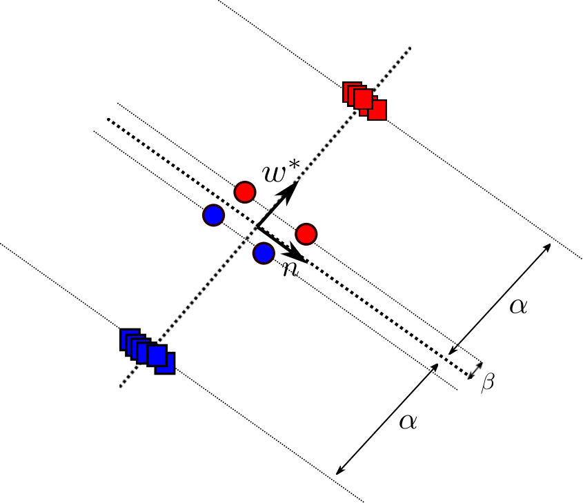
Figure 2: Our synthetic dataset in 2D. Each data-point is $\bm{X}_{i}=[c_{i}\cdot\bm{w^{*}},d_{i}\cdot\bm{n}]\in\mathbb{R}^{4}$ for some $c_{i},d_{i}\in\mathbb{R}.$ We project these points in the 2D space $(\mathrm{span}(\bm{w^{*}}),\mathrm{span}(\bm{n})).$ The feature is $\bm{w^{*}}$ and the noisy patch is in $\mathrm{span}(\bm{n})$. The large margin data (squares) have large component along $\bm{w^{*}}$ and relatively small noise component. The small margin data (circles) have relatively large noise component and thus, these data are well-spread on $\mathrm{span}(\bm{n})$.

Insights on the setting.

The previous experiments suggest that momentum improves generalization in CIFAR-10 while it does not for Gaussian datasets. This means that this generalization improvement must be specific to the data structure and the learning problem. In Section 3, we devise a binary classification problem where the data are linearly separated by a hyperplane directed by the vector $\bm{w^{*}}$ as depicted in Figure 2. We refer to this vector as the feature and the goal is to learn it. Each data-point is a vector constituted of a single signal patch equal to $\theta\bm{w^{*}}$ and of multiple noise patches. For $\mu\ll 1$, we assume that with probability $1-\mu$, the sampled data-point has large margin i.e. $\theta=\alpha\gg 1$ while it has small margin i.e. $\theta=\beta\ll 1$ with probability $\mu$. The noise patches are Gaussian random vectors with small variance. We underline that all the examples share the same feature but differ in their margins. Our dataset can be viewed as an extreme simplification of real-world object-recognition datasets with data of different level of difficulty. Indeed, images are divided into signal patches that are helpful for the classification such as the nose of a dog and noise patches e.g. the background of an image that are uninformative. Besides, the signal patch may be strong i.e. the feature is clearly visible or weak when the feature is indistinguishable e.g. in a car image, the wheel feature is more or less visible depending on the orientation of the car.

Why does GD+M generalize better than GD?

This paper proposes a theory to explain why momentum improves generalization. The following informal theorems characterize the generalization of a 1-hidden layer convolutional neural network trained with GD and GD+M on the aforedescribed dataset. They dramatically simplify Theorem 4.1 and Theorem 4.2 but highlight the intuitions.

Theorem 1.1 (Informal, GD).

There exists a dataset of size $N$ such that a 1-hidden layer (over-parameterized) convolutional network trained with GD:

1. initially only learns the $(1-\mu)N$ large margin data.

2. has small gradient after learning these data.

3. memorizes the remaining small margin data from the $\mu N$ examples.

The model thus reaches zero training loss and well-classifies the large margin data at test. However, it fails to classify the small margin data because of the memorization step during training.

Theorem 1.2 (Informal, GD+M).

There exists a dataset of size $N$ such that a one-hidden layer (over-parameterized) convolutional network trained with GD+M:

1. initially only learns the $(1-\mu)N$ large margin data.

2. has large historical gradients that contain the feature $\bm{w^{*}}$ present in small margin data.

3. keeps learning the feature in the small margin data using its momentum historical gradients.

The model thus reaches zero training error and perfectly classify large and small margin data at test.

Theorem 1.1 and Theorem 1.2 indicate that since the large margin data are dominant, the two models learn in priority these examples to decrease their training losses. Since the training loss is the logistic one, this implies that the gradient terms stemming from the large margin data thus become negligible. Consequently, the current gradient becomes a sum of the small margin data gradients. Thus, it is in the direction of $\beta\bm{w^{*}}$ (signal patch) and Gaussian vectors $\mathbf{g}$ (noise patches). Since $\|\beta\bm{w^{*}}\|_{2}\ll\|\mathbf{g}\|_{2}$, the current gradient is noisy. Therefore, the GD model keeps decreasing its training loss and memorizes the small margin data. On the other hand, contrary to GD, GD+M updates its weights using a weighted average of the historical gradients. In particular, it has large past gradients (stemming from large margin data) that are in the direction $\alpha\bm{w^{*}}$. Therefore, even though the current gradient is noisy, the GD+M uses its historical gradients to learn the small margin data since all the examples share the same feature. We name this process historical feature amplification and believe that it is key to understand why momentum improves generalization.

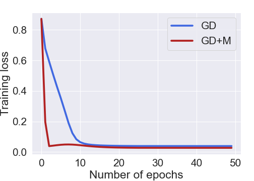
(a)

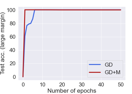
(b)

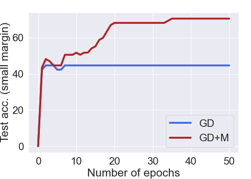
(c)

Figure 3: Training loss (a), accuracy on the large margin (b) and the small margin test data (c) in the setting described in Section 3. While GD and GD+M get zero training loss, GD+M generalizes better on small margin data than GD.

(a)

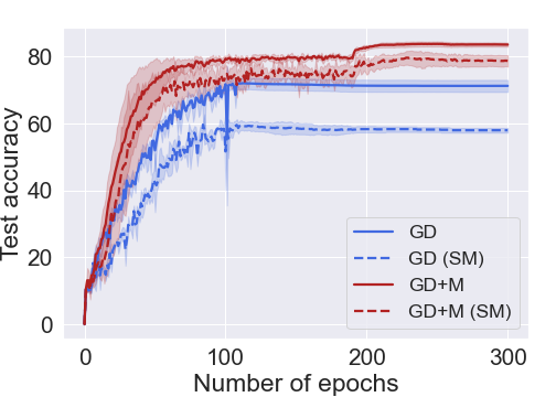
(b)

           

(c)

Figure 4: Training (a) and test (b) accuracy obtained with VGG-19 on the artificially modified CIFAR-10 dataset with small margin data (c). The architectures are trained using GD/GD+M for $300$ epochs to ensure zero training error. Data augmentation and batch normalization are turned off. (SM) stands for the test accuracy obtained by the algorithm on the small margin data. Results are averaged over 5 runs with best scheduled learning rate and weight decay for each individual algorithm separately.

Numerical validation of the theory.

Our theory relies on the ability of momentum to well-classify small margin data. We first perform experiments in our theoretical setting described in Section 3. We set the dimension to $d=30$, the number of training examples to $N=20000$, the test examples to $2000$. Regarding the architecture, we set the number of neurons to $m=5$ and the number of patches to $P=5$. The parameters $\alpha,\beta,\mu$ are set as in Section 3. We refer to stochastic gradient descent optimizer with full batch size as GD/GD+M. Note that for each optimizer, we grid-search over stepsizes to find the best one in terms of test accuracy. We trained the models for 50 epochs. We set the momentum parameter to 0.9. We apply a linear decay learning rate scheduling during training. Figure 3 shows that the models trained with GD and GD+M get zero training loss and well-classify large-margin data at test time. Contrary to GD, GD+M well-classifies small margin data.

Small-margin data in CIFAR-10.

To further validate our theory, we artificially generate small-margin data in CIFAR-10. We first randomly sample 10% of the training and test images. As displayed in 4(c), for each image, we randomly shuffle the RGB channels. We train a VGG-19 without data augmentation nor batch normalization. While the GD and GD+M models reach 100% training accuracy, Figure 4 shows that GD+M gets higher test accuracy than GD. Above all, GD+M generalizes better than GD on small-margin data as the accuracy drop factor for GD+M is $79.47/53.30=1.49$ while for GD, this drop factor is $68.33/34.80=1.96$.

Related Work

Non-convex optimization with momentum.

A long line of work consists in understanding the convergence speed of momentum methods when optimizing non-convex functions. (Mai & Johansson, 2020; Liu et al., 2020; Cutkosky & Mehta, 2020; Defazio, 2020) show that SGD+M reaches a stationary point as fast as SGD under diverse assumptions. Besides, (Leclerc & Madry, 2020) empirically shows that momentum accelerates neural network training for small learning rates and slows it down otherwise. Our paper differs from these works as we work in the batch setting and theoretically investigate the generalization benefits brought by momentum (and not the training ones).

Generalization with momentum.

Momentum-based methods such as SGD+M, RMSProp (Tieleman & Hinton, 2012) and Adam (Kingma & Ba, 2014) are standard in deep learning training since the seminal work of (Sutskever et al., 2013). Although it is known that momentum improve generalization in deep learning, only a few works formally investigate the role of momentum in generalization. (Leclerc & Madry, 2020) empirically report that momentum yields higher generalization when using a large learning rate. However, they assert that this benefit can be obtained by applying an even larger learning rate on vanilla SGD. We suspect that this is due to data augmentation and batch normalization (Ioffe & Szegedy, 2015) which are known to bias the algorithm’s generalization (Bjorck et al., 2018). To our knowledge, our work is the first that theoretically investigates the generalization of momentum in deep learning.

(a)

(b)

Figure 5: Training loss (a) and test accuracy (b) obtained with VGG-19 trained with SGD, SGD+M, GD and GD+M on CIFAR-100. Data augmentation and batch normalization are turned off. Momentum significantly improves generalization whether in the stochastic case (SGD) or in the full batch setting (GD).

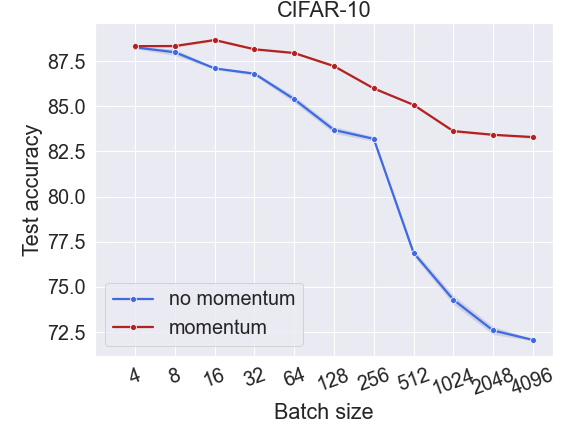
(a)

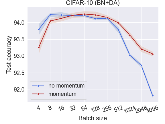
(b)

Figure 6: Test accuracy obtained with a VGG-19 using the stochastic gradient descent optimizer on CIFAR-10 when batch normalization and data augmentation are turned off (a) and on (b). In (a), as the batch size increases, the generalization improvement induced by momentum gets larger. When the network is trained with batch normalization and data augmentation, momentum slightly improves generalization for large batch sizes.

2 Numerical performance of momentum

To evaluate the contribution of momentum to generalization, we conducted extensive experiments on CIFAR-10 and CIFAR-100 (Krizhevsky et al., 2009). We used VGG-19 (Simonyan & Zisserman, 2014) and Resnet-18 (He et al., 2016) as architectures. In this section, we only present the plots obtained with VGG-19 and invite the reader to look at Appendix A for the Resnet-18 experiments.

In all of our experiments, we refer to the stochastic gradient descent optimizer with batch size 128 as SGD/SGD+M and the optimizer with full batch size as GD/GD+M. We turn off data augmentation and batch normalization to isolate the contribution of momentum to the optimization. Note that for each algorithm, we grid-search over stepsizes and momentum parameter to find the best one in terms of test accuracy. We train the models for 300 epochs. The stepsize is decayed by a factor 10 at epochs 190 and 265 during training. All the results are averaged over 5 seeds.

Momentum improves generalization. Figure 5 shows the performance of GD, GD+M, SGD and SGD+M when training a VGG-19 on CIFAR-100. We observe that GD+M/SGD+M consistently outperform GD/SGD. Besides, we highlight that the generalization improvement induced is more significant for GD than for SGD. Similar observations hold for Resnet-18 (see Appendix A).

Influence of batch size. 6(a) shows the test accuracy of a VGG-19 trained on CIFAR-10 with the stochastic gradient descent optimizer on a wide range of batch sizes. We compare the generalization obtained with momentum and without. We remark that momentum does not improve generalization when the batch size is tiny. However, as the batch size increases, the gap between the momentum curve and the no momentum one widens.

Batch normalization and data augmentation. Practitioners usually add batch normalization and data augmentation when training their architectures. 6(b) displays the test accuracy obtained when training a VGG-19 with these two regularizers. We remark that they inhibit the generalization improvement of momentum for small and middle range batch sizes. For large batch sizes, momentum slightly improves generalization. Additional experiments on the influence of batch normalization and data augmentation are in Appendix A.

3 Setting and algorithms

In this section, we introduce our theoretical setting to analyze the implicit bias of momentum. We first formally define the data distribution sketched in the introduction and the neural network model we use to learn it. We finally present the GD and GD+M algorithms.

General notations.

For a matrix $\bm{W}\in\mathbb{R}^{m\times d}$, we denote by $\bm{w}_{r}$ its $r$-th row. For a function $f\colon\mathbb{R}^{m\times d}\rightarrow\mathbb{R}$, we denote by $\nabla_{\bm{w}_{r}}f(W)$ the gradient of $f$ with respect to $w_{r}$ and $\nabla f(\bm{W})$ the gradient with respect to $\bm{W}.$ For an optimization algorithm updating a vector $\bm{w}$, $\bm{w}^{(t)}$ represents its iterate at time $t$. We use $\mathbf{I}_{d}$ for the $d\times d$ identity matrix and $\mathbf{1}_{m}$ the all-ones vector of dimension $m.$ Finally, we use the asymptotic complexity notations when defining the different constants in the paper. We use $\tilde{O},\tilde{\Theta},\tilde{\Omega}$ to hide logarithmic dependency on $d$.

Data distribution.

We define a data distribution $\mathcal{D}$ where each sample consists in an input $\bm{X}$ and a label $y$ such that:

1. Uniformly sample the label $y$ from $\{-1,1\}.$

2. $\bm{X}=(\bm{X}[1],\dots,\bm{X}[P])$ where each patch $\bm{X}[j]\in\mathbb{R}^{d}.$

3. Signal patch: one patch $P(X)\in[P]$ satisfies
   

   $$\bm{X}[P(\bm{X})]=c\bm{w^{*}},\text{where }c\in\mathbb{R},\bm{w^{*}}\in\mathbb{R}^{d},\|\bm{w^{*}}\|_{2}=1.$$

4. $c$ is distributed as $c=\alpha y$ with probability $1-\mu$
   and $c=\beta y$ otherwise.

5. Noisy patches: $\bm{X}[j]\sim\mathcal{N}(0,(\mathbf{I}_{d}-\bm{w^{*}}\bm{w^{*\top}})\sigma^{2}),$
   for $j\in[P]\backslash\{P(\bm{X})\}$.

To keep the analysis simple, the noisy patches are sampled from the orthogonal complement of $\bm{w^{*}}$ and the parameters are set to $\beta=d^{-0.251}$, $\alpha=\mathrm{polylog(d)}\sqrt{d}\beta$, $\sigma=\frac{1}{d^{0.509}}$ and $P\in[2,\mathrm{polylog(d)}]$.

Using this model, we generate a training dataset $\mathcal{Z}=\{(\bm{X}_{i},y_{i})\}_{i\in[N]}$ where $\bm{X}_{i}=(\bm{X}_{i}[j])_{j\in[P]}.$ We set $\mu=1/\mathrm{poly}(d)$ and $N=\Theta\left(\frac{\log\log(d)}{\mu}\right)$. We let $\mathcal{Z}$ to be partitioned in two sets $\mathcal{Z}_{1}$ and $\mathcal{Z}_{2}$ such that $\mathcal{Z}_{1}$ gathers the large margin data while $\mathcal{Z}_{2}$ the small margin ones. Lastly, we define $\hat{\mu}=\frac{|\mathcal{Z}_{2}|}{N}$ the fraction of small margin data.

Learner model.

We use a 1-hidden layer convolutional neural network with cubic activation to learn the training dataset $\mathcal{Z}$. The cubic is the smallest polynomial degree that makes the network non-linear and compatible with our setting. Indeed, the quadratic activation would only output positive labels and mismatch our labeling function. The first layer weights are $\bm{W}\in\mathbb{R}^{m\times d}$ and the second layer is fixed to $\mathbf{1}_{m}.$ Given a input data $\bm{X}$, the output of the model is

$$f_{\bm{W}}(\bm{X})=\sum_{r=1}^{m}\sum_{j=1}^{P}\langle\bm{w}_{r},\bm{X}[j]\rangle^{3}.$$ (CNN)

The number of neurons is set as $m=\mathrm{polylog}(d)$ to ensure that (CNN) is mildly over-parametrized.

Training objective.

We solve the following logistic regression problem for $\lambda\in[0,1/\mathrm{poly}(d)N]$,

(P)

Importance of non-convexity.

When $\lambda>0$, if the loss $\frac{1}{N}\sum_{i=1}^{N}\log\left(1+\exp\left(-y_{i}f_{\bm{W}}(\bm{X}_{i})\right)\right)$ is convex, then there is a unique global optimal solution, so the choice of optimization algorithm does not matter. In our case, due to the non-convexity of the training objective, GD+M converges to a different (approximate) global optimal compared to GD, with better generalization properties.

Test error.

We assess the quality of a predictor $\bm{\widehat{W}}$ using the classical 0-1 loss used in binary classification. Given a sample $(\bm{X},y),$ the individual test (classification) error is defined as $\mathscr{L}(\bm{X},y)=\mathbf{1}\{f_{\bm{\widehat{W}}}(\bm{X})y<0\}.$ While $\mathscr{L}$ measures the error of $f_{\bm{\widehat{W}}}$ on an individual data-point, we are interested in the test error that measures the average loss over data points generated from $\mathcal{D}$ and defined as

$$\mathscr{L}(f_{\bm{\widehat{W}}}):=\mathbb{E}_{(\bm{X},y)\sim\mathcal{D}}[\mathscr{L}(f_{\bm{\widehat{W}}}(\bm{X}),y)].$$ (TE)

Algorithms.

We solve the training problem (P) using GD and GD+M. GD is defined for $t\geq 0$ by

$$\bm{W}^{(t+1)} =\bm{W}^{(t)}-\eta\nabla\widehat{L}(\bm{W}^{(t)}),$$ (GD)

where $\eta>0$ is the learning rate. On the other hand, GD+M is defined by the update rule

$$\begin{cases}\bm{g}^{(t+1)}&=\gamma\bm{g}^{(t)}+(1-\gamma)\nabla\widehat{L}(\bm{W}^{(t)})\\ \bm{W}^{(t+1)}&=\bm{W}^{(t)}-\eta\bm{g}^{(t+1)}\end{cases},$$ (GD+M)

where $\bm{g}^{(0)}=\bm{0}_{m\times d}$ and $\gamma\in(0,1)$ is the momentum factor. We now detail how to set parameters in GD and GD+M.

Parametrization 3.1.

When running GD and GD+M on (P), the number of iterations is any $T\in\left[\mathrm{poly(d)}N/\eta,d^{O(\log d)}/(\eta)\right]$. For both algorithms, the weights $\bm{w}_{1}^{(0)},\dots,\bm{w}_{m}^{(0)}$ are initialized using independent samples from a normal distribution $\mathcal{N}(0,\sigma_{0}^{2}\mathbf{I}_{d})$ where $\sigma_{0}^{2}=\frac{\mathrm{polylog}(d)}{d}.$ The learning rate is set as:

1. GD: the learning rate is reasonable $\eta\in(0,\tilde{O}(1)].$

2. GD+M: the learning rate is large: $\eta=\tilde{\Theta}(1).$

Lastly, the momentum factor is set to $\gamma=1-\frac{\mathrm{polylog}(d)}{d}$.

Our 3.1 matches with the parameters used in practice as the weights are generally initialized from Gaussian with small variance and momentum is set close to 1 (Sutskever et al., 2013).

4 Main results

We now formally state our main theorems regarding the generalization of models trained using (GD) and (GD+M) in the setting described in Section 3. We first introduce some notations.

Main objects.

Let $r\in[m]$, $i\in[N]$, $j\in P\backslash\{P(\bm{X}_{i})\}$ and $t\geq 0.$ Our analysis tracks $\bm{w}_{r}^{(t)}$ the $r$-th weight of the network, $\nabla_{\bm{w}_{r}}\widehat{L}(\bm{W}^{(t)})$ the gradient of $\widehat{L}$ with respect to $\bm{w}_{r}$, $\bm{g}_{r}^{(t)}$ the momentum gradient defined by $\bm{g}_{r}^{(t+1)}=\gamma\bm{g}_{r}^{(t)}+(1-\gamma)\nabla_{\bm{w}_{r}}\widehat{L}(\bm{W}^{(t)})$. We introduce the projection of these objects on the feature $\bm{w^{*}}$ and noise patches $\bm{X}_{i}[j]$:

– Projection on $\bm{w^{*}}$: $c_{r}^{(t)}=\langle\bm{w}_{r}^{(t)},\bm{w^{*}}\rangle$.

  – Projection on $\bm{X}_{i}[j]:$ $\Xi_{i,j,r}^{(t)}=\langle\bm{w}_{r}^{(t)},\bm{X}_{i}[j]\rangle$.

  – Total noise: $\Xi_{i}^{(t)}=\sum_{r=1}^{m}\sum_{j\in[P]\backslash\{P(\bm{X}_{i})\}}y_{i}(\Xi_{i,j,r}^{(t)})^{3}.$

  – Maximum signal: $c^{(t)}=\max_{r\in[m]}c_{r_{\max}}^{(t)}$.

Lastly, we define the negative sigmoid $\mathfrak{S}(x)=1/(1+e^{x}).$

We now provide our first result which states that the learner model trained with GD does not generalize well on $\mathcal{D}$.

Theorem 4.1.

Assume that we run GD on P for $T$ iterations with parameters set as in 3.1. With high probability, the weights learned by GD

1. partially learn $\bm{w^{*}}$: for $r\in[m]$, $|c_{r}^{(T)}|\leq\tilde{O}(1/\alpha).$

2. memorize small margin data: for $i\in\mathcal{Z}_{2},$ $\Xi_{i}^{(T)}\geq\tilde{\Omega}(1).$

Consequently, the training error is smaller than ${O}(\mu/\mathrm{poly}(d))$ and the test error is at least $\tilde{\Omega}(\mu).$

Intuitively, the training process of the GD model is described as follows. Given $|\mathcal{Z}_{1}|\gg|\mathcal{Z}_{2}|$ and our choice of parameters for $\alpha,\beta,\sigma$, the gradient points mainly in the direction of $\bm{w^{*}}$. Therefore, GD eventually learns the feature in $\mathcal{Z}_{1}$ (Lemma 5.1) and the gradients from $\mathcal{Z}_{1}$ quickly become small. Afterwards, the gradient is dominated by the gradients from $\mathcal{Z}_{2}$ (Lemma 5.2). Because $\mathcal{Z}_{2}$ has small margin, the full gradient is now directed by the noisy patches. It implies that GD memorizes noise in $\mathcal{Z}_{2}$ (Lemma 5.4). Since these gradients also control the amount of remaining feature to be learned (Lemma 5.3), we conclude that the GD model partially learns the feature and introduces a huge noise component in the learned weights. We provide a proof sketch of Theorem 4.1 in Section 5. On the other hand, the model trained with GD+M generalizes well on $\mathcal{D}$.

Theorem 4.2.

Assume that we run GD+M on (P) for $T$ iterations with parameters set as in 3.1. With high probability, the weights learned by GD+M

1. at least one of them is correlated with $\bm{w^{*}}$: $c^{(T)}>\tilde{\Omega}(1/\beta).$

2. are barely correlated with noise: for all $r\in[m]$, $i\in[N]$, $j\in[P]\backslash\{P(\bm{X}_{i})\}.$ $|\Xi_{i,j,r}^{(T)}|\leq\tilde{O}(\sigma_{0}).$

The training loss and test error are at most ${O}(\mu/\mathrm{poly}(d)).$

Intuitively, the GD+M model follows this training process. Similarly to GD, it first learns the feature in $\mathcal{Z}_{1}$ (Lemma 6.1). Contrary to GD, the momentum gradient is still highly correlated with $\bm{w^{*}}$ after this step (Lemma 6.2). Indeed, the key difference is that momentum accumulates historical gradients. Since these gradients were accumulated when learning $\mathcal{Z}_{1}$, the direction of momentum gradient is highly biased towards $\bm{w^{*}}$. Therefore, the GD+M model amplifies the feature from these historical gradients to learn the feature in small margin data (Lemma 6.3). Subsequently, the gradient becomes small (Lemma 6.4) and the GD+M model manages to ignore the noisy patches (Lemma 6.5) and learns the feature from both $\mathcal{Z}_{1}$ and $\mathcal{Z}_{2}.$ We provide a proof sketch of Theorem 4.2 in Section 6.

Signal and noise iterates.

Our analysis is built upon a decomposition of the updates (GD) and (GD+M) on $\bm{w^{*}}$ and $\bm{X}_{i}[j]$. The projection of the vanilla and momentum gradients along these directions are

• $\mathscr{G}_{r}^{(t)}=\langle\nabla_{\bm{w}_{r}}\widehat{L}(\bm{W}^{(t)}),\bm{w^{*}}\rangle$ and $\mathcal{G}_{r}^{(t)}=\langle\bm{g}_{r}^{(t)},\bm{w^{*}}\rangle.$

• $\texttt{G}_{i,j,r}^{(t)}=\langle\nabla_{\bm{w}_{r}}\widehat{L}(\bm{W}^{(t)}),\bm{X}_{i}[j]\rangle$ and $G_{i,j,r}^{(t)}=\langle\bm{g}_{r}^{(t)},\bm{X}_{i}[j]\rangle.$

We now define the projected updates as follows:

$$\leavevmode\resizebox{408.68454pt}{}{$\displaystyle\mathcal{G}_{r}^{(t+1)}=\gamma\mathcal{G}_{r}^{(t)}+(1-\gamma)\mathscr{G}_{r}^{(t)}$}$$ (3)

$$\leavevmode\resizebox{399.2946pt}{}{$\displaystyle c_{r}^{(t+1)}=c_{r}^{(t)}-\eta\mathcal{G}_{r}^{(t+1)}$}$$

$$\leavevmode\resizebox{422.77661pt}{}{$\displaystyle G_{i,j,r}^{(t+1)}=\gamma G_{i,j,r}^{(t)}+(1-\gamma)\texttt{G}_{i,j,r}^{(t)}$}$$ (4)

$$\leavevmode\resizebox{413.38667pt}{}{$\displaystyle\Xi_{i,j,r}^{(t+1)}=\Xi_{i,j,r}^{(t)}-G_{i,j,r}^{(t+1)}$}$$

We detail how to use these dynamics to analyze GD+M and GD in Section 5 and Section 6. Our analysis depends on the gradients of $\widehat{L}$ which involve $\mathfrak{S}(x)=\left(1+e^{x}\right)^{-1}.$ We define the derivative of a data-point $i$ as $\ell_{i}^{(t)}=\mathrm{sigmoid}(y_{i}f_{\bm{W}^{(t)}}(\bm{X}_{i}))$, derivatives $\nu_{k}^{(t)}=\frac{1}{N}\sum_{i\in\mathcal{Z}_{k}}\ell_{i}^{(t)}$ for $k\in\{1,2\}$ and full derivative $\nu^{(t)}=\nu_{1}^{(t)}+\nu_{2}^{(t)}$.

5 Analysis of GD

In this section, we provide a proof sketch for Theorem 4.1 that reflects the behavior of GD with $\lambda=0$. A more detailed proof extending to $\lambda>0$ can be found in the Appendix.

Step 1: Learning $\mathcal{Z}_{1}$.

At the beginning of the learning process, the gradient is mostly dominated by the gradients coming from the $\mathcal{Z}_{1}$ samples. Since these data have large margin, the gradient is thus highly correlated with $\bm{w^{*}}$ and $c_{r}^{(t)}$ increases as shown in the following Lemma.

Lemma 5.1.

For all $r\in[m]$ and $t\geq 0$, (1) is simplified as:

$$c_{r}^{(t+1)}\geq c_{r}^{(t)}+\Theta(\eta)\alpha^{3}(c_{r}^{(t)})^{2}\cdot\mathfrak{S}(\textstyle\sum_{s=1}^{t}\alpha^{3}(c_{s}^{(t)})^{3}).$$

Consequently, after $T_{0}=\tilde{\Theta}\left(\frac{1}{\eta\alpha^{3}\sigma_{0}}\right)$ iterations, for all $t\in[T_{0},T]$, we have $c^{(t)}\geq\tilde{\Omega}(1/\alpha)$.

Intuitively, the increment in the update in Lemma 5.1 is non-zero when the sigmoid is not too small which is equivalent to $c^{(t)}\leq\tilde{O}(1/\alpha)$. Therefore, $c^{(t)}$ keeps increasing until reaching this threshold. After this step, the $\mathcal{Z}_{1}$ data have small gradient and therefore, GD has learned these data.

Lemma 5.2.

Let $T_{0}=\tilde{\Theta}\left(\frac{1}{\eta\alpha^{3}\sigma_{0}}\right)$. After $t\in[T_{0},T]$ iterations, $\nu_{1}^{(t)}$ is bounded as $\nu_{1}^{(t)}\leq\tilde{O}\left(\frac{1}{\eta(t-T_{0}+1)\alpha}\right)+\tilde{O}\left(\frac{\beta^{3}}{\alpha}\right)\nu_{2}^{(t)}.$

By our choice of parameter, Lemma 5.2 indicates that the full gradient is dominated by the gradients from $\mathcal{Z}_{2}$ data after $T_{0}=\tilde{\Omega}\left(\frac{1}{\hat{\mu}\eta\alpha}\right).$ Consequently, $\nu_{2}^{(t)}$ also rules the amount of feature learnt by GD.

Lemma 5.3.

Let $T_{0}=\tilde{\Theta}\left(\frac{1}{\eta\alpha^{3}\sigma_{0}}\right)$. For $t\in[T_{0},T]$, (1) becomes $c^{(t+1)}\leq\tilde{O}(1/\alpha)+\tilde{O}(\eta\beta^{3}/\alpha)\sum_{\tau=T_{0}}^{t}\nu_{2}^{(\tau)}.$

Lemma 5.3 implies that quantifying the decrease rate of $\nu_{2}^{(t)}$ provides an estimate on the quantity of feature learnt by the model. We remark that $\nu_{2}^{(t)}=\mathfrak{S}(\beta^{3}\sum_{s=1}^{m}(c_{s}^{(t)})^{3}+\Xi_{i}^{(t)})$ for some $i\in\mathcal{Z}_{2}$. We thus need to determine whether the feature or the noise terms dominates in the sigmoid.

Step 2: Memorizing $\mathcal{Z}_{2}$.

We now show that the total correlation between the weights and the noise in $\mathcal{Z}_{2}$ data increases until being large.

Lemma 5.4.

Let $i\in\mathcal{Z}_{2}$, $j\in[P]\backslash\{P(\bm{X}_{i})\}$ and $r\in[m]$. For $t\geq 0$, (2) is simplified as:

$$y_{i}\Xi_{i,j,r}^{(t+1)} \geq y_{i}\Xi_{i,j,r}^{(0)}+\frac{\tilde{\Theta}(\eta\sigma^{2}d)}{N}\sum_{\tau=0}^{t}(\Xi_{i,j,r}^{(\tau)})^{2}\mathfrak{S}(\Xi_{i}^{(\tau)})$$

$$-\tilde{O}(P\sigma^{2}\sqrt{d}/\alpha).$$

Let $T_{1}=\tilde{\Theta}\left(\frac{N}{\sigma_{0}\sigma\sqrt{d}\sigma^{2}d}\right)$. Consequently, for $t\in[T_{1},T]$, we have $\Xi_{i}^{(t)}\geq\tilde{\Omega}(1)$. Thus, GD memorizes.

By Lemma 5.4, the noise $\Xi_{i}^{(t)}$ dominates in $\nu_{2}^{(t)}$. Consequently, the algorithm memorizes the $\mathcal{Z}_{2}$ data which implies a fast decay of $\nu_{2}^{(t)}$.

Lemma 5.5.

Let $T_{1}=\tilde{\Theta}\left(\frac{N}{\sigma_{0}\sigma\sqrt{d}\sigma^{2}d}\right)$. For $t\in[T_{1},T]$, we have $\sum_{\tau=0}^{t}\nu_{2}^{(\tau)}\leq\tilde{O}(1/\eta\sigma_{0}).$

Combining Lemma 5.5 and Lemma 5.3, we prove that GD partially learns the feature.

Lemma 5.6.

For $t\leq T$, we have $c^{(t)}\leq\tilde{O}(1/\alpha)$.

Lemma 5.4 and Lemma 5.6 respectively yield the first two items in Theorem 4.1. Bounds on the training loss and test errors are obtained by plugging these results in (P) and (TE).

6 Analysis of GD+M

In this section, we provide a proof sketch for Theorem 4.2 that reflects the behavior of GD+M with $\lambda=0$. A proof extending to $\lambda>0$ can be found in the Appendix.

Step 1: Learning $\mathcal{Z}_{1}$.

Similarly to GD, by our initialization choice, the early gradients and so, momentum gradients are large. They are in the span of $\bm{w^{*}}$ and therefore, the GD+M model also increases its correlation with $\bm{w^{*}}$.

Lemma 6.1.

For all $r\in[m]$ and $t\geq 0$, as long as $c^{(t)}\leq\tilde{O}(1/\alpha)$, the momentum update (3) is simplified as:

$$-\mathcal{G}_{r}^{(t+1)}=-\gamma\mathcal{G}_{r}^{(t)}+(1-\gamma)\Theta(\alpha^{3})(c_{r}^{(t)})^{2}$$

Consequently, after $\mathcal{T}_{0}=\tilde{\Theta}\left(\frac{1}{\sigma_{0}\alpha^{2}}+\frac{1}{1-\gamma}\right)$ iterations, for all $t\in[\mathcal{T}_{0},T]$, we have $c^{(t)}\geq\tilde{\Omega}(1/\alpha)$.

Step 2: Learning $\mathcal{Z}_{2}$.

Contrary to GD, GD+M has a large momentum that contains $\bm{w^{*}}$ after Step 1.

Lemma 6.2.

Let $\mathcal{T}_{0}=\tilde{\Theta}\left(\frac{1}{\sigma_{0}\alpha^{3}}+\frac{1}{1-\gamma}\right)$. Let $r_{\max}=\mathrm{argmax}_{r\in[m]}c_{r}^{(t)}$. For $t\in[\mathcal{T}_{0},T]$, we have $\mathcal{G}_{r_{\max}}^{(t)}\geq\tilde{\Omega}(\sqrt{1-\gamma}/\alpha).$

Lemma 6.2 hints an important distinction between GD and GD+M: while the current gradient along $\bm{w^{*}}$ is small at time $\mathcal{T}_{0},$ the momentum gradient stores historical gradients that are spanned by $\bm{w^{*}}$. It amplifies the feature present in previous gradients to learn the feature in $\mathcal{Z}_{2}$.

Lemma 6.3.

Let $\mathcal{T}_{0}=\tilde{\Theta}\left(\frac{1}{\sigma_{0}\alpha^{3}}+\frac{1}{1-\gamma}\right)$. After $\mathcal{T}_{1}=\mathcal{T}_{0}+\tilde{\Theta}\left(\frac{1}{1-\gamma}\right)$ iterations, for $t\in[\mathcal{T}_{1},T]$, we have $c^{(t)}\geq\tilde{\Omega}\left(\frac{1}{\sqrt{1-\gamma}\alpha}\right).$ Our choice of parameter in Section 3, this implies $c^{(t)}\geq\tilde{\Omega}(1/\beta).$

Lemma 6.3 states that at least one of the weights that is highly correlated with the feature compared to GD where $c^{(t)}=\tilde{O}(1)$. This result implies that $\nu^{(t)}$ converges fast.

Lemma 6.4.

Let $\mathcal{T}_{0}=\tilde{\Theta}\left(\frac{1}{\eta\sigma_{0}\alpha^{3}}+\frac{1}{1-\gamma}\right)$. After $\mathcal{T}_{1}=\mathcal{T}_{0}+\tilde{\Theta}\left(\frac{1}{1-\gamma}\right)$ iterations, for $t\in[\mathcal{T}_{1},T]$, $\nu^{(t)}\leq\tilde{O}\left(\frac{1}{\eta(t-\mathcal{T}_{1}+1)\beta}\right)$.

With this fast convergence, Lemma 6.4 implies that the correlation of the weights with the noisy patches does not have enough time to increase and thus, remains small.

Lemma 6.5.

Let $i\in[N]$, $j\in[P]\backslash\{P(\bm{X}_{i})\}$ and $r\in[m]$. For $t\geq 0,$ (4) can be rewritten as $|G_{i,j,r}^{(t+1)}|\leq\gamma|G_{i,j,r}^{(t)}|+(1-\gamma)\tilde{O}(\sigma_{0}^{2}\sigma^{4}d^{2})\nu^{(t)}.$ As a consequence, after $t\in[\mathcal{T}_{1},T]$ iterations, we thus have $|\Xi_{i,j,r}^{(t)}|\leq\tilde{O}(\sigma_{0}\sigma\sqrt{d}).$

Lemma 6.3 and Lemma 6.5 respectively yield the two first items in Theorem 4.2.

7 Discussion

Our work is a first step towards understanding the algorithmic regularization of momentum and leaves room for improvements. We constructed a data distribution where historical feature amplification may explain the generalization improvement of momentum. However, it would be interesting to understand whether this phenomenon is the only reason or whether there are other mechanisms explaining momentum’s benefits. An interesting setting for this question is NLP where momentum is used to train large models as BERT (Devlin et al., 2018). Lastly, our analysis is in the batch setting to isolate the generalization induced by momentum. It would be interesting to understand how the stochastic noise and the momentum together contribute to the generalization of a neural network.

Appendix A Additional Experiments

In this section, we present additional experiments to further strengthen our empirical results. We verify on Resnet-18 that momentum induces generalization improvement when trained without batch normalization and data augmentation. We then check that when these two regualizers are used, momentum does not improve generalization. We then confirm on Resnet-18 that the generalization improvement gets larger as the batch size increases. Then, we provide the performance of SGD and SGD+M on the Gaussian experiment introduced in the introduction. Lastly, we give additional plots showing that momentum allows to well-classify small margin data as mentioned at the end of the introduction.

A.1 Experiments with Resnet-18

Figure 7 displays the training loss and test accuracy obtained by training a Resnet-18 on CIFAR-10 and CIFAR-100. Similarly to the case where we trained a VGG-19, momentum significantly improves generalization whether in the stochastic case (SGD) or in the full batch setting (GD).

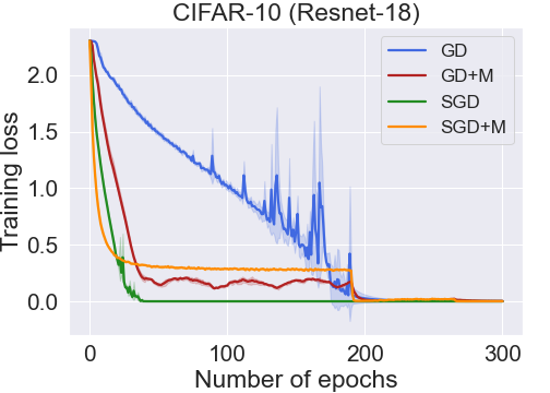
(a)

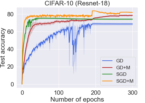
(b)

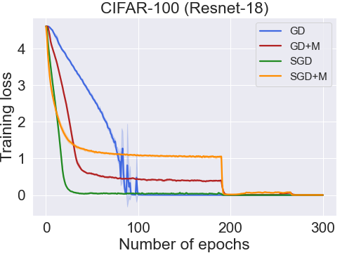
(c)

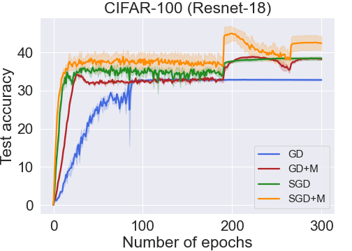
(d)

Figure 7: Training loss and test accuracy obtained with Resnet-18 trained with SGD, SGD+M, GD and GD+M on CIFAR-10 (a-b) and CIFAR-100 (c-d). Data augmentation and batch normalization are turned off.

A.2 Influence of the batch size

Figure 8 shows the test accuracy obtained with a Resnet-18 using the stochastic gradient descent optimizer on CIFAR-10. Similarly to the VGG-19 experiment in Section 2, the generalization improvement induced by momentum gets larger as the batch size increases.

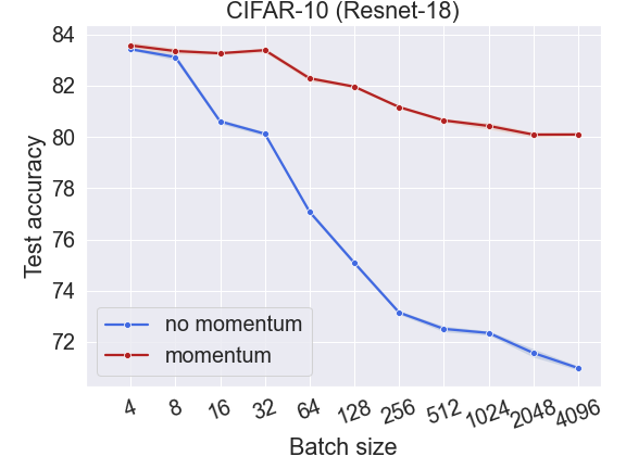
Figure 8: Test accuracy obtained with a Resnet-18 using the stochastic gradient descent optimizer on CIFAR-10 when batch normalization and data augmentation are turned off.

A.3 Influence of batch normalization and data augmentation

As mentioned in Section 2, batch normalization and data augmentation significantly reduce the generalization improvement induced by momentum. We further confirm this observation in Figure 9 and Figure 10.

(a)

(b)

(c)

(d)

Figure 9: Training loss and test accuracy obtained with VGG-19 trained with SGD, SGD+M, GD and GD+M on CIFAR-10 (a-b) and CIFAR-100 (c-d). Data augmentation and batch normalization are turned on.

(a)

(b)

(c)

(d)

Figure 10: Training loss and test accuracy obtained with Resnet-18 trained with SGD, SGD+M, GD and GD+M on CIFAR-10 (a-b) and CIFAR-100 (c-d). Data augmentation and batch normalization are turned on.

A.4 Synthetic Gaussian data experiments

We provide a complete table with mean and standard deviations obtained by using different student networks to learn the Gaussian synthetic experiment mentioned in the introduction.

	Linear	1-MLP	2-MLP	1-CNN	2-CNN
1-MLP	$93.48\pm 0.13$	$92.32\pm 0.50$	$84.30\pm 0.82$	$94.18\pm 0.42$	$76.04\pm 0.29$
2-MLP	$93.45\pm 0.22$	$91.02\pm 0.41$	$83.82\pm 0.43$	$94.14\pm 0.47$	$75.50\pm 0.35$
1-CNN	$92.21\pm 0.16$	$92.31\pm 0.57$	$83.39\pm 0.48$	$94.39\pm 0.17$	$79.44\pm 0.58$
2-CNN	$91.04\pm 0.48$	$91.51\pm 0.40$	$82.44\pm 0.45$	$93.91\pm 0.35$	$80.86\pm 0.92$

(a)

	Linear	1-MLP	2-MLP	1-CNN	2-CNN
1-MLP	$93.25\pm 0.22$	$92.18\pm 0.53$	$83.68\pm 0.74$	$94.12\pm 0.43$	$76.12\pm 0.22$
2-MLP	$92.85\pm 0.34$	$91.78\pm 0.62$	$83.25\pm 0.70$	$94.20\pm 0.13$	$75.56\pm 0.33$
1-CNN	$92.34\pm 0.21$	$92.33\pm 0.64$	$83.44\pm 0.52$	$94.39\pm 0.15$	$78.32\pm 0.34$
2-CNN	$91.22\pm 0.39$	$91.56\pm 0.52$	$82.12\pm 0.55$	$93.79\pm 0.25$	$78.56\pm 0.64$

(b)

	Linear	1-MLP	2-MLP	1-CNN	2-CNN
1-MLP	$93.58\pm 0.32$	$92.56\pm 0.62$	$85.74\pm 0.56$	$94.18\pm 0.42$	$76.06\pm 0.39$
2-MLP	$93.51\pm 0.25$	$91.82\pm 0.83$	$85.33\pm 0.81$	$94.14\pm 0.33$	$75.33\pm 0.47$
1-CNN	$92.42\pm 0.05$	$92.03\pm 0.53$	$84.57\pm 0.47$	$94.22\pm 0.18$	$80.02\pm 0.45$
2-CNN	$91.54\pm 0.37$	$92.04\pm 0.48$	$83.81\pm 0.47$	$93.95\pm 0.31$	$82.86\pm 0.59$

(c)

	Linear	1-MLP	2-MLP	1-CNN	2-CNN
1-MLP	$93.56\pm 0.28$	$92.82\pm 0.26$	$84.65\pm 0.45$	$94.16\pm 0.42$	$76.01\pm 0.33$
2-MLP	$93.24\pm 0.34$	$92.26\pm 0.76$	$84.27\pm 0.79$	$94.24\pm 0.40$	$75.04\pm 0.47$
1-CNN	$92.50\pm 0.05$	$91.68\pm 0.72$	$83.39\pm 0.44$	$94.07\pm 0.035$	$78.92\pm 0.41$
2-CNN	$91.61\pm 0.41$	$91.94\pm 0.54$	$83.70\pm 0.37$	$93.89\pm 0.33$	$80.50\pm 0.45$

(d)

Table 2: Test accuracy obtained using GD (a), GD+M (b), SGD (c) and GD+M (d) on a Gaussian synthetic dataset trained using neural network with ReLU activations. The training dataset consists in 500 data points in dimension 50 and test set in 5000 points. The student networks are trained for 1000 epochs to ensure zero training error. Results averaged over 3 runs.

A.5 Additional justification for the theory

In this section, we present further experiments to consolidate the experiment on the artificially decimated CIFAR-10 dataset described in the introduction.

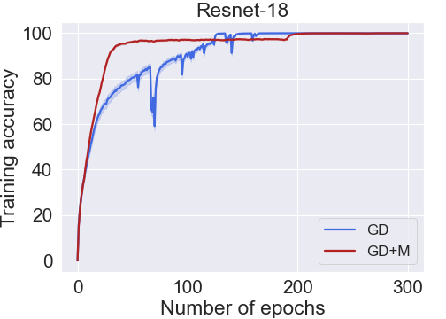
(a)

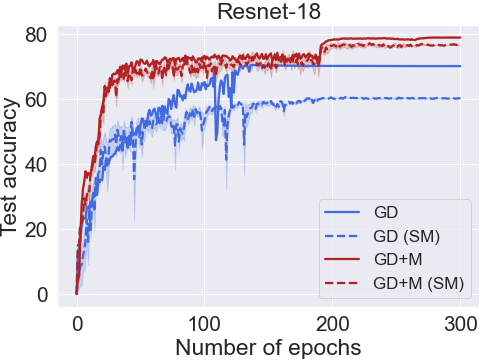
(b)

(c)

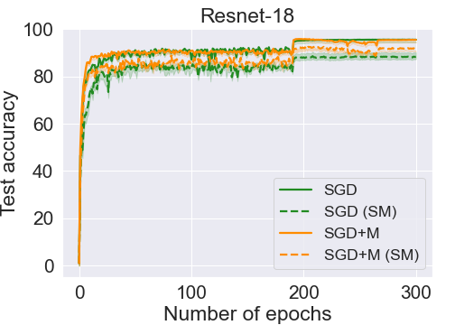
(d)

Figure 11: Training and test accuracy obtained with Resnet-18 on the artificially modified CIFAR-10 dataset with small margin data. The architectures are trained using GD/GD+M (a-b) and SGD/SGD+M (c-d) for $300$ epochs to ensure zero training error. Data augmentation and batch normalization are turned off.

In 11(a), we observe that using a Resnet-18, momentum still improves generalization on the small margin images.In 11(d) and 12(b), we see that using stochastic updates lead SGD to classify small margin images as well as SGD+M. Lastly, Figure 13 and Figure 14 show that batch normalization and data augmentation also reduce the generalization improvement of momentum: GD/SGD perform similarly as well as GD+M/SGD+M on the small margin data.

(a)

(b)

Figure 12: Training and test accuracy obtained with VGG-19 on the artificially modified CIFAR-10 dataset with small margin data. The architectures are trained using SGD/SGD+M (a-b). Data augmentation and batch normalization are turned off.

(a)

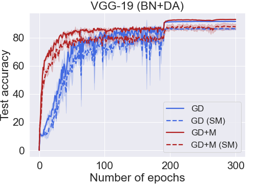
(b)

(c)

(d)

Figure 13: Training and test accuracy obtained with VGG-19 on the artificially modified CIFAR-10 dataset with small margin data. The architectures are trained using GD/GD+M (a-b) and SGD/SGD+M (c-d). Data augmentation and batch normalization are turned on.

(a)

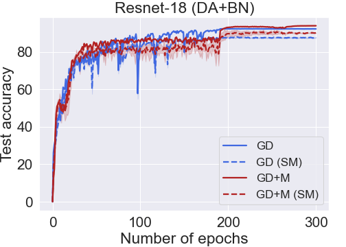
(b)

(c)

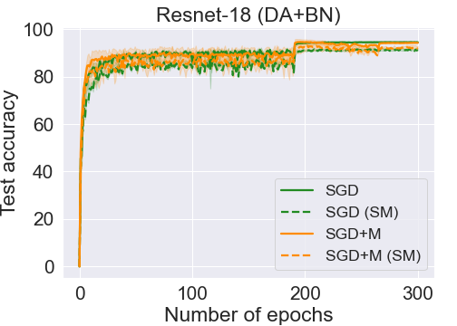
(d)

Figure 14: Training and test accuracy obtained with Resnet-18 on the artificially modified CIFAR-10 dataset with small margin data. The architectures are trained using GD/GD+M (a-b) and SGD/SGD+M (c-d). Data augmentation and batch normalization are turned on.

blabla

blabla

Appendix B Additional related work

Momentum in convex setting.

GD+M (a.k.a. heavy ball or Polyak momentum) consists in using an exponentially weighted average of the past gradients to update the weights. For convex functions near a strict twice-differentiable minimum, GD+M is optimal regarding local convergence rate (Polyak, 1963, 1964; Nemirovskij & Yudin, 1983; Nesterov, 2003). However, it may fail to converge globally for general strongly convex twice-differentiable functions (Lessard et al., 2015) and is no longer optimal for the class of smooth convex functions. In the stochastic setting, GD+M is more sensitive to noise in the gradients; that is, to preserve their improved convergence rates, significantly less noise is required (d’Aspremont, 2008; Schmidt et al., 2011; Devolder et al., 2014; Kidambi et al., 2018). Finally, other momentum methods are extensively used for convex functions such as Nesterov’s accelerated gradient (Nesterov, 1983). Our paper focuses on the use of GD+M and contrary to the aforementioned papers, our setting is non-convex. Besides, we mainly focus on the generalization of the model learned by GD and GD+M when both methods converge to global optimal. Contrary to the non-convex case, generalization is disentangled from optimization for (strictly) convex functions.

Algorithmic regularization.

The question we address concerns algorithmic regularization which characterizes the generalization of an optimization algorithm when multiple global solutions exist in over-parametrized models (Soudry et al., 2018; Lyu & Li, 2019; Ji & Telgarsky, 2019; Chizat & Bach, 2020; Gunasekar et al., 2018; Arora et al., 2019). This regularization arises in deep learning mainly due to the non-convexity of the objective function. Indeed, this latter potentially creates multiple global minima scattered in the space that vastly differ in terms of generalization. Algorithmic regularization is induced by and depends on many factors such as learning rate and batch size (Goyal et al., 2017; Hoffer et al., 2017; Keskar et al., 2016; Smith et al., 2018), initialization (Allen-Zhu & Li, 2020), adaptive step-size (Kingma & Ba, 2014; Neyshabur et al., 2015; Wilson et al., 2017), batch normalization (Arora et al., 2018; Hoffer et al., 2019; Ioffe & Szegedy, 2015) and dropout (Srivastava et al., 2014; Wei et al., 2020). However, none of these works theoretically analyzes the regularization induced by momentum.

Appendix C Notations

In this section, we introduce the different notations used in the proofs. We start by defining the notations that appear for GD and GD+M. We first consider the case when $\lambda=0$, we will extend the proof to $\lambda>0$ in section H

C.1 Notations for GD and GD+M

Our paper rely on the notions of signal and noise components of the iterates.

– Signal intensity: $\theta=\alpha$ if $i\in\mathcal{Z}_{1}$ and $\beta$ otherwise.

– Signal: $c_{r}^{(t)}=\langle\bm{w^{*}},\bm{w}_{r}^{(t)}\rangle$ for $r\in[m].$

– Max signal: $c^{(t)}=c_{r_{\max}}^{(t)}$ where $r_{\max}\in\mathrm{argmax}_{r\in[m]}c_{r}^{(t)}$.

– Noise: $\Xi_{i,j,r}^{(t)}=\langle\bm{w}_{r}^{(t)},\bm{X}_{i}[j]\rangle$ for $i\in[N]$ and $j\in[P]\backslash\{P(\bm{X}_{i})\}.$

– Max noise: ${\Xi}_{\max}^{(t)}=\max_{i\in[N],j\not=P(\bm{X}_{i}),r\in[m]}|\Xi_{i,j,r}^{(t)}|^{2}.$

– Total noise: $\Xi_{i}^{(t)}=\sum_{r\in[m],j\in[P],j\not=P(\bm{X}_{i})}y_{i}\left(\Xi_{i,j,r}^{(t)}\right)^{3}.$

We also use the following notations when dealing with the loss function and its gradient.

– Signal loss: $\widehat{\mathcal{L}}^{(t)}(a)=\log\left(1+\exp\left(-\sum_{r=1}^{m}(c_{r}^{(t)})^{3}a^{3}\right)\right)$ for $a\in\mathbb{R}$.

– Noise loss: $\widehat{\mathcal{L}}^{(t)}(\Xi_{i}^{(t)})=\log\left(1+\exp\left(-\Xi_{i}^{(t)}\right)\right)$.

– Negative sigmoid function: $\mathfrak{S}(x)=(1+\exp(x))^{-1}$, for $x\in\mathbb{R}.$

– Signal derivative: $\widehat{\ell}^{(t)}(a)=\mathfrak{S}\left(\sum_{r=1}^{m}(c_{r}^{(t)})^{3}a^{3}\right),$ for $a\in\mathbb{R}.$

– Noise derivative: $\widehat{\ell}^{(t)}(\Xi_{i}^{(t)})=\mathfrak{S}(\Xi_{i}^{(t)}).$

– Derivative: $\ell_{i}^{(t)}=\mathfrak{S}\left(-\sum_{r=1}^{m}\sum_{j=1}^{P}y_{i}\langle\bm{w}_{r}^{(t)},\bm{X}_{i}[j]\rangle^{3}\right)$, for $i\in[N].$

– $\mathcal{Z}_{k}$ derivative: $\nu_{k}^{(t)}=\frac{1}{N}\sum_{i\in\mathcal{Z}_{k}}\ell_{i}^{(t)}$ for $k\in\{1,2\}.$

– Full derivative: $\nu^{(t)}=\nu_{1}^{(t)}+\nu_{2}^{(t)}.$

– Gradient on signal: $\mathscr{G}_{r}^{(t)}=\langle\nabla_{\bm{w}_{r}}\widehat{L}(\bm{W}^{(t)}),\bm{w^{*}}\rangle$ for $r\in[m].$

– Gradient on noise: $\texttt{G}_{i,j,r}^{(t)}=\langle\nabla_{\bm{w}_{r}}\widehat{L}(\bm{W}^{(t)}),\bm{X}_{i}[j]\rangle$ for $i\in[N]$, $j\in[P]\backslash\{P(\bm{X}_{i})\}$ and $r\in[m].$

– Gradient on normalized noise: $\mathrm{G}_{r}^{(t)}=\left\langle\nabla_{\bm{w}_{r}}\widehat{L}(\bm{W}^{(t)}),\bm{{\mathchoice{\raisebox{0.0pt}{$\displaystyle\chi$}}{\raisebox{0.0pt}{$\textstyle\chi$}}{\raisebox{0.0pt}{$\scriptstyle\chi$}}{\raisebox{0.0pt}{$\scriptscriptstyle\chi$}}}}\right\rangle,$ for $r\in[m]$, where $\bm{{\mathchoice{\raisebox{0.0pt}{$\displaystyle\chi$}}{\raisebox{0.0pt}{$\textstyle\chi$}}{\raisebox{0.0pt}{$\scriptstyle\chi$}}{\raisebox{0.0pt}{$\scriptscriptstyle\chi$}}}}=\frac{\frac{1}{N}\sum_{i\in\mathcal{Z}_{2}}\sum_{j\neq P(\bm{X}_{i})}\bm{X}_{i}[j]}{\|\frac{1}{N}\sum_{i\in\mathcal{Z}_{2}}\sum_{j\neq P(\bm{X}_{i})}\bm{X}_{i}[j]\|_{2}}.$

C.2 Notations specific to GD+M

We now introduce the notations that only appear in the proofs involving GD+M.

– Momentum gradient oracle: $\bm{g}_{r}^{(t)}=\gamma\bm{g}_{r}^{(t-1)}+(1-\gamma)\nabla_{\bm{w}_{r}}\widehat{L}(\bm{W}^{(t)})$ for $r\in[m].$

– Signal momentum: $\mathcal{G}_{r}^{(t)}:=\langle\bm{g}_{r}^{(t)},\bm{w^{*}}\rangle$ for $r\in[m].$

– Max signal momentum: $\mathcal{G}^{(t)}=\mathcal{G}_{r_{\max}}^{(t)}$, where $r_{\max}=\mathrm{argmax}_{r\in[m]}c_{r}^{(t)}.$

– Noise momentum: $G_{i,j,r}^{(t)}=\langle\bm{g}_{r}^{(t)},\bm{X}_{i}[j]\rangle$ for $i\in[N]$, $j\in[P]\backslash\{P(\bm{X}_{i})\}$ and $r\in[m].$

Appendix D Induction hypotheses

We prove our main result using an induction. More specifically, we make the following assumptions for every time $t\leq T.$

Induction hypothesis D.1 (Bound on the noise component for GD).

Throughout the training process using GD for $t\leq T$, we maintain that:

1. (Large signal data have small noise component). For every $i\in\mathcal{Z}_{1}$, for every $j\in[P]\backslash\{P(\bm{X}_{i})\}$ and $r\in[m],$ we maintain:

   $$|\Xi_{i,j,r}^{(t)}|\leq\tilde{O}(\sigma_{0}\sigma\sqrt{d}).$$ (5)

2. (Small signal data have large noise component). For every $i\in\mathcal{Z}_{2}$, for every $j\in[P]\backslash\{P(\bm{X}_{i})\}$ and $r\in[m],$ we have:

   $$|\Xi_{i,j,r}^{(t)}|\leq\tilde{O}(1),\quad y_{i}\Xi_{i,j,r}^{(t)}\geq-\tilde{O}(\sigma_{0}\sigma\sqrt{d}).$$ (6)

Induction hypothesis D.2 (Bound on the signal component for GD).

Throughout the training process using GD for $t\leq T$, the signal component is bounded for every $r\in[m]$ as

$$-\tilde{O}(\sigma_{0})\leq c_{r}^{(t)}\leq\widetilde{O}(1/\alpha).$$

Induction hypothesis D.3 (Max noise is bounded by max signal component).

Throughout the training process using GD for $t\leq T$, we maintain:

$$\alpha\min\{\kappa,\alpha^{2}(c^{(t)})^{2}\}\geq\tilde{\Omega}\left({\Xi}_{\max}^{(t)}\right),$$

where $\kappa=\tilde{O}(1).$

Induction hypothesis D.4 (Bound on the noise component for GD+M).

Throughout the training process using GD+M for $t\leq T$, for every $i\in[N]$, for every $j\in[P]\backslash\{P(\bm{X}_{i})\}$, we have that:

$$|\Xi_{i,j,r}^{(t)}|\leq\tilde{O}(\sigma_{0}\sigma\sqrt{d})$$ (7)

Induction hypothesis D.5 (Bound on the signal component for GD+M).

Throughout the training process using GD+M for $t\leq T$, for $r\in[m]$, we have that:

$$-\tilde{O}(\sigma_{0})\leq c_{r}^{(t)}\leq\widetilde{O}(1/\beta).$$ (8)

In what follows, we assume these induction hypotheses for $t<T$ to prove our generalization results. We then prove these hypotheses for $t+1.$

Appendix E Gradients and updates

In this section, we first derive the gradient of the loss $\widehat{L}$. We then provide its projection on $\bm{\bm{w^{*}}}$ (signal gradient) and on $\bm{X}_{i}[j]$ (noise gradient). We first derive the gradient of the loss $\widehat{L}.$

Lemma E.1 (Gradient of $\widehat{L}$).

For $t\geq 0$ and $r\in[m]$, the gradient of the loss $\widehat{L}$ with respect to $\bm{w}_{r}$ is:

$$\nabla_{\bm{w}_{r}}\widehat{L}(\bm{W}^{(t)}) =-\frac{3}{N}\left[\left(\sum_{i\in\mathcal{Z}_{1}}\alpha^{3}\ell_{i}^{(t)}+\sum_{i\in\mathcal{Z}_{2}}\beta^{3}\ell_{i}^{(t)}\right)(c_{r}^{(t)})^{2}\bm{w^{*}}+\sum_{i=1}^{N}\sum_{j\neq P(X_{i})}\ell_{i}^{(t)}(\Xi_{i,j,r}^{(t)})^{2}\bm{X}_{i}[j]\right].$$

Proof of Lemma E.1.

. We derive $\widehat{L}$ with respect to $\bm{w}_{r}$ and obtain:

$$\nabla_{\bm{w}_{r}}\widehat{L}(\bm{W}^{(t)}) =-\frac{3}{N}\sum_{i=1}^{N}\sum_{j=1}^{P}\frac{y_{i}\langle\bm{w}_{r}^{(t)},\bm{X}_{i}[j]\rangle^{2}}{1+\exp(f_{\bm{W}^{(t)}}(X_{i}))}\bm{X}_{i}[j].$$ (9)

By rewriting (9), we obtain the desired result. ∎

E.1 Signal gradient

To track the signal learnt by our models, we compute the signal gradient which is the projection of the gradient on $\bm{w^{*}}.$

Lemma E.2 (Signal gradient).

For all $t\geq 0$ and $r\in[m]$, the signal gradient is:

$$-\mathscr{G}_{r}^{(t)} =\frac{3}{N}\left(\sum_{i\in\mathcal{Z}_{1}}\alpha^{3}\ell_{i}^{(t)}+\sum_{i\in\mathcal{Z}_{2}}\beta^{3}\ell_{i}^{(t)}\right)(c_{r}^{(t)})^{2}.$$

Proof of Lemma E.2.

We obtain the desired result by projecting the gradient from Lemma E.1 on $\bm{w^{*}}$ and using $\bm{X}_{i}[j]\perp\bm{w^{*}}.$ ∎

E.2 Noise gradient

To prove the memorization of GD and the non-memorization of GD+M, we also need to compute the noise gradient which is the projection of the gradient $\nabla_{\bm{w}_{r}}\widehat{L}$ on $\bm{X}_{i}[j].$

Lemma E.3 (Noise gradient).

For all $t\geq 0$, $i\in[N]$ and $j\in[P]\backslash\{P(X_{i})\}$ and $r\in[m]$, the noise gradient is:

$$-\texttt{G}_{i,j,r}^{(t)} =\frac{3}{N}\ell_{i}^{(t)}(\Xi_{i,j,r}^{(t)})^{2}\|\bm{X}_{i}[j]\|_{2}^{2}$$

$$+\frac{3}{N}\sum_{k\neq P(X_{i})}\ell_{i}^{(t)}(\Xi_{i,k,r}^{(t)})^{2}\langle\bm{X}_{i}[k],\bm{X}_{i}[j]\rangle$$

$$+\frac{3}{N}\sum_{a\neq i}\sum_{k\neq P(X_{a})}\ell_{a}^{(t)}(\Xi_{a,k,r}^{(t)})^{2}\langle\bm{X}_{a}[k],\bm{X}_{i}[j]\rangle.$$

Proof of Lemma E.3.

Similarly to Lemma E.2, we obtain the desired result by projecting the gradient from Lemma E.1 on $\bm{X}_{i}[j]$ and using $\bm{X}_{i}[j]\perp\bm{w^{*}}.$ ∎

Remark 1.

The gradient in Lemma E.1 involve sigmoid terms $\ell_{i}^{(t)}$. In several parts of the proof, we focus on the time where these terms are small. We consider that the sigmoid term is small for a $\kappa$ such that

$$\sum_{\tau=0}^{T}\frac{1}{1+\exp(\kappa)} \leq\tilde{O}(1)\implies\kappa\geq\log(\tilde{\Omega}(T))\iff\kappa\geq\tilde{\Omega}(1).$$ (10)

Intuitively, (10) means that the sum of the sigmoid terms for all time steps is bounded (up to a logarithmic dependence).

Appendix F Learning with GD

In this section, we detail the proofs of the lemmas in Section 5 and Theorem 4.1. We first characterize the dynamics of the signal $c_{r}^{(t)}$ in subsection F.1. We then analyze the dynamics of the noise $\Xi_{i,j,r}^{(t)}$ in subsection F.2 and show the memorization of the GD model. We finally prove Theorem 4.1 in subsection F.3 and the induction hypotheses in subsection F.4.

F.1 Learning signal with GD

To track the amount of signal learnt by GD, we make use of the following update.

Lemma F.1 (Signal update).

For all $t\geq 0$ and $r\in[m]$, the signal update (1) is equal:

$$c_{r}^{(t+1)} =c_{r}^{(t)}+3\eta\left(\alpha^{3}\nu_{1}^{(t)}+\beta^{3}\nu_{2}^{(t)}\right)(c_{r}^{(t)})^{2}.$$

Consequently, it satisfies:

$$\tilde{\Theta}(\eta)(1-\hat{\mu})\alpha^{3}\widehat{\ell}^{(t)}(\alpha)(c_{r}^{(t)})^{2}\leq c_{r}^{(t+1)}-c_{r}^{(t)}\leq\tilde{\Theta}(\eta)\left((1-\hat{\mu})\alpha^{3}\widehat{\ell}^{(t)}(\alpha)+\beta^{3}\nu_{2}^{(t)}\right)(c_{r}^{(t)})^{2}.$$ (11)

Proof of Lemma F.1.

The signal update is obtained by using (1) and the signal gradient (Lemma E.2). This yields

$$c_{r}^{(t+1)} =c_{r}^{(t)}+\frac{3\eta}{N}\left(\sum_{i\in\mathcal{Z}_{1}}\alpha^{3}\ell_{i}^{(t)}+\sum_{i\in\mathcal{Z}_{2}}\beta^{3}\ell_{i}^{(t)}\right)(c_{r}^{(t)})^{2}.$$ (12)

To obtain the desired lower bound, we first drop the sum over $\mathcal{Z}_{2}$ in (12). Then, for $i\in\mathcal{Z}_{1}$, we apply Lemma I.1 to get $\ell_{i}^{(t)}=\Theta(1)\widehat{\ell}^{(t)}(\alpha)$.

To obtain the desired upper bound, we apply the same reasoning as above to bound the $\mathcal{Z}_{1}$ term. ∎

F.1.1 Early stages of the learning process $t\in[0,T_{0}]$: learning $\mathcal{Z}_{1}$ data

Since $\bm{w}_{r}^{(0)}\sim\mathcal{N}(0,\sigma_{0}^{2}\mathbf{I}_{d})$ with $\sigma_{0}$ small, the sigmoid terms $\widehat{\ell}^{(t)}(\alpha)$ and $\ell_{i}^{(t)}$ in the signal update are large at early iterations. As $c_{r}^{(t)}$ is non-decreasing (by Lemma F.1), $\widehat{\ell}^{(t)}(\alpha)$ eventually becomes small at a time $T_{0}>0.$ As mentioned in Remark 1, the sigmoid term $\mathfrak{S}(x)$ is small when $x\geq\kappa\geq\tilde{\Omega}(1)$. We therefore simplify (12) for $t\in[0,T_{0}]$.

Lemma F.2 (Signal update at early iterations).

Let $T_{0}>0$ the time where there exists $s\in[m]$ such that $c_{s}^{(t)}\geq\tilde{\Omega}(1/\alpha)$. Then, for $t\in[0,T_{0}]$ and for all $r\in[m]$, the signal update is simplified as:

$$\Theta(\eta)(1-\hat{\mu})\alpha^{3}(c_{r}^{(t)})^{2}\leq c_{r}^{(t+1)}-c_{r}^{(t)}\leq\Theta(\eta)\left((1-\hat{\mu})\alpha^{3}+\hat{\mu}\beta^{3}\right)(c_{r}^{(t)})^{2}.$$ (13)

Proof of Lemma F.2.

For $t\in[0,T_{0}]$, we know that for all $s\in[m]$, we have $c_{s}^{(t)}\leq\frac{\kappa}{m^{1/3}\alpha}$. Therefore, we have

$$\frac{1}{1+\exp(\tilde{\Omega}(1))}\leq\widehat{\ell}^{(t)}(\alpha)=\frac{1}{1+\exp\left(\sum_{s=1}^{m}\alpha^{3}(c_{s}^{(t)})^{3}\right)}\leq 1.$$ (14)

From Remark 1, the sigmoid is small when it is equal to $\frac{1}{1+\exp(\tilde{\Omega}(1))}$. Thus, for $t\in[T_{0},T]$, we have:

$$\widehat{\ell}^{(t)}(\alpha)=\Theta(1).$$ (15)

Plugging (15) in the left-hand side of (11) yields the desired lower bound.

To get the upper bound, we start from the right-hand side of (11). We upper bound $\frac{1}{N}\sum_{i\in\mathcal{Z}_{2}}\ell_{i}^{(t)}\leq\hat{\mu}$ since $\ell_{i}^{(t)}\leq 1.$ Moreover, we use (15) to upper bound the $\widehat{\ell}^{(t)}(\alpha)$ term. ∎

We now prove Lemma 5.1 that quantifies the amount of signal learnt by GD when the derivative is large.

See 5.1

Proof of Lemma 5.1.

Let $r\in[m]$. From Lemma F.2, the signal update for $t\in[0,T_{0}]$ is

$$\begin{cases}c_{r}^{(t+1)}\leq c_{r}^{(t)}+A(c_{r}^{(t)})^{2}\\ c_{r}^{(t+1)}\geq c_{r}^{(t)}+B(c_{r}^{(t)})^{2}\end{cases},$$ (16)

where $A$ and $B$ are respectively defined as:

$$A :=\tilde{\Theta}(\eta)\left((1-\hat{\mu})\alpha^{3}+\hat{\mu}\beta^{3}\right),$$

$$B :=\tilde{\Theta}(\eta)(1-\hat{\mu})\alpha^{3}.$$

Now, we would like to find the time $T_{0}$ where $c_{r}^{(t)}\geq\tilde{\Omega}(1/\alpha).$ This time exists as $c_{r}^{(t)}$ is non-decreasing. To this end, we apply the Tensor Power method (Lemma K.15). This lemma only applies to non-negative sequences. Since we initialize the weights $\bm{w}_{r}^{(0)}\sim\mathcal{N}(0,\sigma_{0}^{2}\mathbf{I}_{d})$, we have $c_{r}^{(0)}\sim\mathcal{N}(0,\sigma_{0}^{2}).$ Since all the $w_{r}^{(0)}$’s are i.i.d. so do the $c_{r}^{(0)}$’s. Therefore, the probability that at least one of the $c_{r}^{(0)}$ is non-negative is $1-(1/2)^{m}=1-o(1).$ We thus conclude that with high probability, there exist an index $r\in[m]$ such that $c_{r}^{(0)}\geq 0.$ Among the possible indices $r$ that satisfy this inequality, we now focus on $r=r_{\max}$ where $r_{\max}\in\mathrm{argmax}\;c_{r}^{(0)}$.

Setting $\upsilon=\tilde{\Theta}(1/\alpha)$ in Lemma K.15, we deduce that the time $T_{0}$ is

$$T_{0}=\frac{\tilde{\Theta}(1)}{\eta\alpha^{3}\sigma_{0}}+\frac{\tilde{\Theta}(1)\left((1-\hat{\mu})\alpha^{3}+\hat{\mu}\beta^{3}\right)}{(1-\hat{\mu})\alpha^{3}}\left\lceil\frac{-\log(\tilde{\Theta}(\sigma_{0}\alpha))}{\log(2)}\right\rceil$$

∎

We now prove Lemma 5.2. It states that since the signal $c^{(t)}$ has significantly increased, the $\mathcal{Z}_{1}$ derivative $\nu_{1}^{(t)}$ is now small. Before proving this result, we introduce an auxiliary Lemma.

Lemma F.3 (Lower bound on the signal update).

Run GD on the loss function $\widehat{L}(W).$ After $T_{0}=\tilde{\Theta}\left(\frac{1}{\eta\alpha^{3}\sigma_{0}}\right)$ iterations, the signal update is satisfies for $t\geq t_{0}$

$$c^{(t+1)}\geq c^{(t)}+\eta\tilde{\Omega}(\alpha)\nu_{1}^{(t)}.$$

Proof of Lemma F.3 .

From Lemma F.1, we know that

$$c^{(t+1)} \geq c^{(t)}+\tilde{\Theta}(\eta)\nu_{1}^{(t)}\alpha^{3}(c^{(t)})^{2}.$$ (17)

Plugging $c^{(t)}\geq\tilde{\Omega}(1/\alpha)$ (Lemma 5.1) in (17), we obtain the desired result. ∎

See 5.2

Proof of Lemma 5.2.

From Lemma F.3, we deduce an upper bound on $\nu_{1}^{(t)}$:

$$\nu_{1}^{(t)}\leq\tilde{O}\left(\frac{1}{\eta\alpha}\right)(c^{(t+1)}-c^{(t)}).$$ (18)

On the other hand, using Lemma E.2, the signal difference is bounded as:

$$c^{(t+1)}-c^{(t)} \leq\sum_{r=1}^{m}c_{r}^{(t+1)}-c_{r}^{(t)}$$

$$\leq(1-\hat{\mu})\Theta(\eta\alpha)\sum_{r=1}^{m}(\alpha c_{r}^{(t)})^{2}\widehat{\ell}^{(t)}(\alpha)+\hat{\mu}\Theta(\eta\beta^{3})\sum_{r=1}^{m}(c_{r}^{(t)})^{2}\nu_{2}^{(t)}.$$ (19)

By applying D.1 in (19) and using $m=\tilde{\Theta}(1)$, we obtain:

$$c^{(t+1)}-c^{(t)} \leq(1-\hat{\mu})\Theta(\eta\alpha)\sum_{r=1}^{m}(\alpha c_{r}^{(t)})^{2}\widehat{\ell}^{(t)}(\alpha)+\hat{\mu}\tilde{O}(\eta\beta^{3})\nu_{2}^{(t)}.$$ (20)

We now bound (20) by a loss term by applying Lemma K.20. Using Lemma 5.1 and D.2, we have:

$$0<\tilde{\Omega}(1/\alpha)\leq\tilde{\Omega}(1/\alpha)-m\tilde{O}(\sigma_{0})\leq c^{(t)}-\sum_{r\neq r_{\max}}c_{r}^{(t)}\leq\sum_{r=1}^{m}\alpha c_{r}^{(t)}\leq m\tilde{O}(1)\leq\tilde{O}(1).$$ (21)

We can now apply Lemma K.20 and get:

$$\sum_{r=1}^{m}(\alpha c_{r}^{(t)})^{2}\widehat{\ell}^{(t)}(\alpha)\leq\frac{20m\alpha e^{m\tilde{O}(\sigma_{0})}}{\tilde{\Omega}(1)}\widehat{\mathcal{L}}^{(t)}(\alpha)\leq\tilde{O}(\alpha)\widehat{\mathcal{L}}^{(t)}(\alpha).$$ (22)

Plugging (22) in (20) yields:

$$c^{(t+1)}-c^{(t)} \leq(1-\hat{\mu})\tilde{O}(\eta\alpha^{2})\widehat{\mathcal{L}}^{(t)}(\alpha)+\hat{\mu}\tilde{O}(\eta\beta^{3})\nu_{2}^{(t)}.$$ (23)

Combining (18) and (23), we thus obtain:

$$\nu_{1}^{(t)}\leq\tilde{O}\left(\frac{1}{\alpha}\right)\left((1-\hat{\mu})\tilde{O}(\alpha^{2})\widehat{\mathcal{L}}^{(t)}(\alpha)+\hat{\mu}\tilde{O}(\beta^{3})\nu_{2}^{(t)}\right).$$ (24)

From Lemma I.7, we have the convergence rate of $\widehat{\mathcal{L}}^{(t)}(\alpha)$. We use it to bound $\nu_{1}^{(t)}.$

The bound on $\nu^{(t)}$ is obtained by using its definition $\nu^{(t)}=\nu_{1}^{(t)}+\nu_{2}^{(t)}$. ∎

F.1.2 Late stages of learning process $t\in[T_{0},T]$: amount of learnt signal controlled by $\mathcal{Z}_{2}$ derivative

We earlier proved that after $T_{0}$ iterations, the signal $c^{(t)}$ learnt by the GD model significantly increases until making $\nu_{1}^{(t)}$ small. We therefore need to rewrite the signal update in this case.

Lemma F.4 (Rewriting of signal update).

For $t\in[T]$, the maximal signal $c^{(t)}$ updates as:

$$c^{(t+1)}-c^{(t)}\leq\Theta(\eta)\left(\alpha\nu_{1}^{(t)}\min\{\kappa,(c^{(t)})^{2}\alpha^{2}\}+\frac{\beta^{3}}{\alpha^{2}}\nu_{2}^{(t)}\right).$$

Proof of Lemma F.4.

From the signal update given by Lemma F.1, we know that:

$$c^{(t+1)} =c^{(t)}+\frac{3\eta\alpha}{N}\sum_{i\in\mathcal{Z}_{1}}(\alpha c^{(t)})^{2}\ell_{i}^{(t)}+3\eta\beta^{3}\nu_{2}^{(t)}(c^{(t)})^{2}.$$ (25)

To obtain the desired result, we need to prove for $i\in\mathcal{Z}_{1}$:

$$(\alpha c^{(t)})^{2}\ell_{i}^{(t)} \leq\Theta(1)\min\{\kappa,\alpha^{2}(c^{(t)})^{2}\}.$$ (26)

Indeed, we remark that:

$$(\alpha c^{(t)})^{2}\ell_{i}^{(t)} =\frac{\alpha^{3}(c^{(t)})^{2}}{1+\exp\left(\alpha^{3}\sum_{s=1}^{m}(c_{s}^{(t)})^{3}+\Xi_{i}^{(t)}\right)}.$$ (27)

By using D.1 and D.2, (27) is bounded as:

$$(\alpha c^{(t)})^{2}\ell_{i}^{(t)} =\frac{\alpha^{3}(c^{(t)})^{2}}{1+\exp\left(\alpha^{3}(c^{(t)})^{3}+\alpha^{3}\sum_{s\neq r_{\max}}(c_{s}^{(t)})^{3}+\Xi_{i}^{(t)}\right)}$$

$$\leq\frac{\alpha^{3}(c^{(t)})^{2}}{1+\exp\left(\alpha^{3}(c^{(t)})^{3}-\tilde{O}(m\alpha^{3}\sigma_{0}^{3})-\tilde{O}(mP(\sigma\sigma_{0}\sqrt{d})^{3})\right)}$$

$$=\frac{\Theta(\alpha)(\alpha c^{(t)})^{2}}{1+\exp((\alpha c^{(t)})^{3})}.$$ (28)

Using Remark 1, the sigmoid term in (F.1.2) becomes small when $\alpha c^{(t)}\geq\kappa^{1/3}$. To summarize, we have:

$$(\alpha c^{(t)})^{2}\ell_{i}^{(t)} =\begin{cases}0&\text{if }\alpha c^{(t)}\geq\kappa^{1/3}\\ (\alpha c^{(t)})^{2}\ell_{i}^{(t)}&\text{otherwise}\end{cases}.$$ (29)

(29) therefore implies $(\alpha c^{(t)})^{2}\ell_{i}^{(t)}\leq\Theta(1)\min\{\kappa^{2/3},(\alpha c^{(t)})^{2}\}$ which implies (26).

Besides, we use D.2 to bound $(c^{(t)})^{2}$ in the right-hand side of (25). ∎

We now show that once $\nu_{1}^{(t)}$ is small, the amount of learnt signal is controlled by $\nu_{2}^{(t)}$ .

See 5.3

Proof of Lemma 5.3.

Let $\tau\in[T_{0},T)$. From Lemma F.4, we know that:

$$c^{(\tau+1)}-c^{(\tau)}\leq\Theta(\eta)\left(\alpha\nu_{1}^{(\tau)}\min\{\kappa,(c^{(\tau)})^{2}\alpha^{2}\}+\frac{\beta^{3}}{\alpha^{2}}\nu_{2}^{(\tau)}(c^{(\tau)})^{2}\right)$$ (30)

Let $t\in[\tau,T)$. We now sum up (30) for $\tau=T_{0},\dots,t$ and obtain:

$$c^{(t+1)}\leq c^{(T_{0})}+\Theta(\eta\alpha)\sum_{\tau=T_{0}}^{t}\nu_{1}^{(\tau)}\min\{\kappa,(c^{(\tau)})^{2}\alpha^{2}\}+\frac{\Theta(\eta\beta^{3})}{\alpha^{2}}\sum_{\tau=T_{0}}^{t}\nu_{2}^{(\tau)}.$$ (31)

We now plug the bound on $\nu_{1}^{(t)}$ from Lemma 5.2 in (31). This implies:

$$c^{(t+1)}\leq c^{(T_{0})}+\sum_{\tau=T_{0}}^{t}\frac{\tilde{O}(1)}{\tau-T_{0}+1}+\tilde{O}(\eta\beta^{3})\left(1+\frac{1}{\alpha^{2}}\right)\sum_{\tau=T_{0}}^{t}\nu_{2}^{(\tau)}.$$ (32)

Plugging $\sum_{\tau}1/\tau\leq\tilde{O}(1)$ and $c^{(T_{0})}\leq\tilde{O}(1/\alpha)$ (D.2) in (32), we obtain:

$$c^{(t+1)}\leq\frac{\tilde{O}(1)}{\alpha}+\frac{\tilde{O}(\eta\beta^{3})}{\alpha^{2}}\sum_{\tau=T_{0}}^{t}\nu_{2}^{(\tau)}.$$

∎

F.2 Memorization process of GD

Lemma 5.2 shows that after $T_{0}$ iterations, the gradient is controlled by $\nu_{2}^{(t)}$. In this section, we show that this yields the GD model to memorize.

F.2.1 Memorizing $\mathcal{Z}_{2}$ ($t\in[0,T_{1}]$)

Using Lemma F.1, we simplify the noise update.

Lemma F.5 (Noise update).

Let all $t\geq 0$, $i\in[N]$, $j\in[P]\backslash\{P(\bm{X}_{i})\}$ and $r\in[m]$. Then, with probability at least $1-o(1)$, the noise update (2) is bounded as

$$\left|y_{i}\Xi_{i,j,r}^{(t+1)}-y_{i}\Xi_{i,j,r}^{(t)}-\frac{\tilde{\Theta}(\eta\sigma^{2}d)}{N}\ell_{i}^{(t)}(\Xi_{i,j,r}^{(t)})^{2}\right|\leq\frac{\tilde{\Theta}(\eta\sigma^{2}\sqrt{d})}{N}\sum_{a=1}^{N}\ell_{a}^{(t)}\sum_{k\neq P((\bm{X}_{a})}(\Xi_{a,k,r}^{(t)})^{2}.$$ (33)

Proof of Lemma F.5.

Let $i\in[N]$, $j\in[P]\backslash\{P(\bm{X}_{i})\}$ and $r\in[m]$. From Lemma E.3, we know that the noise update satisfies:

$$\begin{split}y_{i}\Xi_{i,j,r}^{(t+1)}&=y_{i}\Xi_{i,j,r}^{(t)}+\frac{3\eta}{N}\ell_{i}^{(t)}(\Xi_{i,j,r}^{(t)})^{2}\|\bm{X}_{i}[j]\|_{2}^{2}+\frac{3\eta}{N}\ell_{i}^{(t)}\sum_{\begin{subarray}{c}k\neq P(X_{i})\\ k\neq j\end{subarray}}(\Xi_{i,k,r}^{(t)})^{2}\langle\bm{X}_{i}[k],\bm{X}_{i}[j]\rangle\\ &+\frac{3\eta}{N}\sum_{a\neq i}\ell_{a}^{(t)}\sum_{k\neq P(\bm{X}_{a})}(\Xi_{a,k,r}^{(t)})^{2}\langle\bm{X}_{a}[k],\bm{X}_{i}[j]\rangle.\end{split}$$ (34)

We now apply Lemma K.5 and Lemma K.7 to respectively bound $\|\bm{X}_{i}[j]\|_{2}^{2}$ and $\langle\bm{X}_{a}[k],\bm{X}_{i}[j]\rangle$ in (34) and obtain the desired result. ∎

In the next lemma, we further simplify the noise update from Lemma F.5.

Lemma F.6 (Sum of noise updates).

Let $i\in\mathcal{Z}_{2}$, $j\in[P]\backslash\{P(\bm{X}_{i})\}$ and $r\in[m].$ Let $\mathfrak{T}=\tilde{\Theta}\left(\frac{P\sigma^{2}\sqrt{d}}{\eta\beta^{3}\hat{\mu}}\right)$. For $t\leq\mathfrak{T}$, the noise update satisfies:

$$\left|y_{i}\Xi_{i,j,r}^{(t+1)}-y_{i}\Xi_{i,j,r}^{(0)}-\frac{\tilde{\Theta}(\eta\sigma^{2}d)}{N}\sum_{\tau=0}^{t}\widehat{\ell}^{(\tau)}(\Xi_{i}^{(\tau)})(\Xi_{i,j,r}^{(\tau)})^{2}\right|\leq\tilde{O}\left(\frac{P\sigma^{2}\sqrt{d}}{\alpha}\right).$$ (35)

Proof of Lemma F.6.

Let $i\in\mathcal{Z}_{2}$, $j\in[P]\backslash\{P(\bm{X}_{i})\}$ and $r\in[m]$. Our starting point is Lemma I.4 which states that:

$$\left|y_{i}\Xi_{i,j,r}^{(t)}-y_{i}\Xi_{i,j,r}^{(0)}-\frac{\eta\tilde{\Theta}(\sigma^{2}d)}{N}\sum_{\tau=0}^{t-1}\ell_{i}^{(\tau)}(\Xi_{i,j,r}^{(\tau)})^{2}\right| \leq\tilde{O}\left(\frac{P\sigma^{2}\sqrt{d}}{\alpha}\right)+\tilde{O}\left(\frac{\eta\beta^{3}}{\alpha}\right)\sum_{j=0}^{t}\nu_{2}^{(j)}.$$ (36)

Since $t\leq\mathfrak{T}=\tilde{\Theta}\left(\frac{P\sigma^{2}\sqrt{d}}{\eta\beta^{3}\hat{\mu}}\right)$, we bound the second sum term in (36) as:

$$\tilde{O}\left(\frac{\eta\beta^{3}}{\alpha}\right)\sum_{j=0}^{t}\nu_{2}^{(j)} \leq\tilde{O}\left(\frac{\eta\beta^{3}}{\alpha}\right)\hat{\mu}t\leq\tilde{O}\left(\frac{\eta\beta^{3}\hat{\mu}\mathfrak{T}}{\alpha}\right)\leq\tilde{O}\left(\frac{P\sigma^{2}\sqrt{d}}{\alpha}\right).$$ (37)

From (37), we deduce that

$$\left|y_{i}\Xi_{i,j,r}^{(t)}-y_{i}\Xi_{i,j,r}^{(0)}-\frac{\eta\tilde{\Theta}(\sigma^{2}d)}{N}\sum_{\tau=0}^{t-1}\ell_{i}^{(\tau)}(\Xi_{i,j,r}^{(\tau)})^{2}\right| \leq\tilde{O}\left(\frac{P\sigma^{2}\sqrt{d}}{\alpha}\right).$$ (38)

Lastly, we know from Lemma I.2 that $\ell_{i}^{(\tau)}=\Theta(1)\widehat{\ell}^{(t)}(\Xi_{i}^{(\tau)})$. Plugging this in (38) yields the desired result. ∎

Since $\bm{w}_{r}^{(0)}\sim\mathcal{N}(0,\sigma_{0}^{2}\mathbf{I}_{d})$ with $\sigma_{0}$ small, the sigmoid terms $\widehat{\ell}^{(t)}(\Xi_{i}^{(t)})$ in the noise update are large at early iterations. After a certain time $T_{1}>0$, there exist an index $s\in[m]$ such that $\Xi_{i,j,s}^{(t)}$ becomes large and $\widehat{\ell}^{(t)}(\Xi_{i}^{(t)})$ eventually becomes small. We therefore simplify (35) for $t\in[0,T_{1}].$

Lemma F.7 (Noise update at early iterations).

Let $i\in\mathcal{Z}_{2}$ and $j\in[P]\backslash\{P(\bm{X}_{i})\}$. Let $T_{1}>0$ be the time where there exists $s\in[m]$ such that $\Xi_{i,j,s}^{(t)}\geq\tilde{\Omega}(1)$. Then, for $t\in[0,T_{1}]$ and for all $r\in[m]$, the noise update is simplified as:

$$\left|y_{i}\Xi_{i,j,r}^{(t+1)}-y_{i}\Xi_{i,j,r}^{(0)}-\frac{\tilde{\Theta}(\eta\sigma^{2}d)}{N}\sum_{\tau=0}^{t}(\Xi_{i,j,r}^{(\tau)})^{2}\right|\leq\tilde{O}\left(\frac{P\sigma^{2}\sqrt{d}}{\alpha}\right).$$ (39)

Proof of Lemma F.7.

Let $t\leq T_{1}$. We assume for now that $T_{1}\leq\mathfrak{T}=\tilde{\Theta}\left(\frac{P\sigma^{2}\sqrt{d}}{\eta\beta^{3}\hat{\mu}}\right)$ and will check this hypothesis in the proof of Lemma 5.4. Let $i\in\mathcal{Z}_{2}$, $j\in[P]\backslash\{P(\bm{X}_{i})\}$ and $r\in[m]$. From Lemma F.6, we know that

$$\left|y_{i}\Xi_{i,j,r}^{(t+1)}-y_{i}\Xi_{i,j,r}^{(0)}-\frac{\tilde{\Theta}(\eta\sigma^{2}d)}{N}\sum_{\tau=0}^{t}\widehat{\ell}^{(\tau)}(\Xi_{i}^{(\tau)})(\Xi_{i,j,r}^{(\tau)})^{2}\right|\leq\tilde{O}\left(\frac{P\sigma^{2}\sqrt{d}}{\alpha}\right).$$ (40)

From Remark 1, we know that $\widehat{\ell}^{(\tau)}(\Xi_{i}^{(\tau)})$ is small when $\Xi_{i}^{(\tau)}\geq\kappa\geq\tilde{\Omega}(1).$ To have this condition, it is sufficient that there exists an index $s\in[m]$ such that $y_{i}\Xi_{i,j,s}^{(\tau)}\geq\tilde{\Omega}(1).$ Indeed, by using D.1, we have:

$$\Xi_{i}^{(t)} =(y_{i}\Xi_{i,j,s}^{(t)})^{3}+\sum_{s=1}^{m}\sum_{k\neq P(\bm{X}_{i})}(y_{i}\Xi_{i,k,s}^{(t)})^{3}\geq\tilde{\Omega}(1)-\tilde{O}(mP(\sigma\sigma_{0}\sqrt{d})^{3})\geq\tilde{\Omega}(1).$$

Therefore, for $t\in[0,T_{1}]$ and $\tau\leq t$, we have $\widehat{\ell}^{(\tau)}(\Xi_{i}^{(\tau)})=\Theta(1)$. In this case, the noise update (40) is:

$$\left|y_{i}\Xi_{i,j,r}^{(t+1)}-y_{i}\Xi_{i,j,r}^{(0)}-\frac{\tilde{\Theta}(\eta\sigma^{2}d)}{N}\sum_{\tau=0}^{t}(\Xi_{i,j,r}^{(\tau)})^{2}\right|\leq\tilde{O}\left(\frac{P\sigma^{2}\sqrt{d}}{\alpha}\right).$$ (41)

∎

Lemma F.7 indicates that $y_{i}\Xi_{i,j,r}^{(t)}$ is not non-decreasing but overall, this quantity gets large over time. We now want to determine the time $T_{1}$ where one of the $y_{i}\Xi_{i,j,r}^{(t)}$ becomes large.

Lemma F.8.

Let $i\in\mathcal{Z}_{2}$, $j\in[P]\backslash\{P(\bm{X}_{i}\}$ and $T_{1}=\tilde{\Theta}\left(\frac{N}{\sigma_{0}\sigma\sqrt{d}\sigma^{2}d}\right).$ After $T_{1}$ iterations, there exists $s\in[m]$ such that $\Xi_{i,j,s}^{(t)}\geq\tilde{\Omega}(1).$

Proof of Lemma F.8.

Lemma F.7 indicates that the noise iterate satisfies for $t\in[0,T_{1}]$:

$$\begin{aligned} \begin{cases}y_{i}\Xi_{i,j,r}^{(t)}\geq y_{i}\Xi_{i,j,r}^{(0)}+A\sum_{\tau=0}^{t-1}(\Xi_{i,j,r}^{(\tau)})^{2}-C\\ y_{i}\Xi_{i,j,r}^{(t)}\leq y_{i}\Xi_{i,j,r}^{(0)}+A\sum_{\tau=0}^{t-1}(\Xi_{i,j,r}^{(\tau)})^{2}+C\end{cases}\end{aligned},$$ (42)

where $A,C>0$ are constants defined as

$$A=\frac{\tilde{\Theta}(\eta\sigma^{2}d)}{N},\quad C=\tilde{O}\left(\frac{P\sigma^{2}\sqrt{d}}{\alpha}\right).$$ (43)

To find $T_{1}$, we apply the Tensor Power method (Lemma K.16) to (42). We initialize the weights $\bm{w}_{r}^{(0)}\sim\mathcal{N}(0,\sigma_{0}^{2}\mathbf{I}_{d})$ and $\bm{X}_{i}[j]\sim\mathcal{N}(0,\sigma^{2}\mathbf{I}_{d})$. Therefore, we have $\mathbb{P}[y_{i}\Xi_{i,j,r}^{(0)}\geq 0]=1/2$. Since all the $w_{r}^{(0)}$’s are i.i.d. so do the $\Xi_{i,j,r}^{(0)}$’s. Therefore, the probability that at least one of the $\Xi_{i,j,r}^{(0)}$ is non-negative is $1-(1/2)^{m}=1-o(1).$ We thus conclude that with high probability, there exist an index $r\in[m]$ such that $y_{i}\Xi_{i,j,r}^{(0)}\geq\Omega(\sigma\sigma_{0}\sqrt{d})\geq\Omega(C)$. In what follows, we focus on such index $r$.

Setting the constants $A,C$ as in (43) and $\upsilon=\tilde{O}(1)$, the time $T_{1}$ obtained with the Tensor Power method is

$$T_{1} =\frac{21N}{\tilde{\Theta}(\eta\sigma^{2}d)y_{i}\Xi_{i,j,r}^{(0)}}+\frac{8N}{\tilde{\Theta}(\eta\sigma^{2}d)(y_{i}\Xi_{i,j,r}^{(0)})}\left\lceil\frac{\log\left(\frac{\tilde{O}(1)}{y_{i}\Xi_{i,j,r}^{(0)}}\right)}{\log(2)}\right\rceil.$$

We thus obtain $T_{1}=\tilde{\Theta}\left(\frac{N}{\eta\sigma^{2}d\sigma_{0}\sigma\sqrt{d}}\right).$ We indeed verify that $T_{1}\leq\mathfrak{T}$ since $\tilde{\Theta}\left(\frac{N}{\eta\sigma^{2}d\sigma_{0}\sigma\sqrt{d}}\right)\ll\tilde{\Theta}\left(\frac{NP\sigma^{2}\sqrt{d}}{\eta\beta^{3}\hat{\mu}}\right).$

∎

See 5.4

Proof of Lemma 5.4.

The simplified (2) update is obtained from Lemma F.6. Besides, we know that $T_{1}$ is the first time where there exists $s\in[m]$ such that $\Xi_{i,j,s}^{(t)}\geq\tilde{\Omega}(1).$ As explained in the proof of Lemma F.7, $\Xi_{i,k,s}^{(t)}\geq\tilde{\Omega}(1)$ implies that $\Xi_{i}^{(t)}\geq\tilde{\Omega}(1).$ We can therefore apply Lemma F.8 to obtain the aimed result.

∎

F.2.2 Late stages of memorization $t\in[T_{1},T]$: convergence to a minimum

We proved in the previous section that after $T_{1}$ iterations, the amount of noise memorized by the GD model significantly increases. We want to show that after this phase, $\nu_{2}^{(t)}$ is well-controlled.

Lemma F.9 (Bound on $\mathcal{Z}_{2}$ derivative at late iterations).

Let $T_{1}=\tilde{\Theta}\left(\frac{N}{\sigma_{0}\sigma\sqrt{d}\sigma^{2}d}\right)$. For $t\in[T_{1},T]$, we have $\sum_{\tau=T_{1}}^{t}\nu_{2}^{(\tau)}\leq\tilde{O}\left(\frac{1}{\eta\sigma_{0}}\right).$

Proof of Lemma F.9 .

In Lemma F.8, we proved that after $T_{1}$ iterations, for all $i\in\mathcal{Z}_{2}$ and $j\in[P]\backslash\{P(\bm{X}_{i})\}$, there exists $s\in[m]$ such that $y_{i}\Xi_{i,j,s}^{(t)}\geq\tilde{\Omega}(1).$ Therefore, for $t\in[T_{1},T]$, there exists $s\in[m]$ such that the noise update (from Lemma I.4) satisfies:

$$\sum_{\tau=T_{1}}^{t}\nu_{2}^{(\tau)} \leq\tilde{O}\left(\frac{1}{\eta\sigma^{2}d}\right)\sum_{i\in\mathcal{Z}_{2}}y_{i}(\Xi_{i,j,s}^{(t+1)}-\Xi_{i,j,s}^{(T_{1})})$$ (44)

$$+\tilde{O}\left(\frac{P}{\alpha\eta\sqrt{d}}\right)+\tilde{O}\left(\frac{\beta^{3}}{\alpha\sigma^{2}d}\right)\sum_{j=T_{1}}^{t-1}\nu_{2}^{(j)}.$$

On the other hand, from Lemma I.4, we know that for all $r\in[m]$:

$$\sum_{i\in\mathcal{Z}_{2}}y_{i}(\Xi_{i,j,r}^{(t+1)}-\Xi_{i,j,r}^{(T_{1})}) \leq\frac{\eta\tilde{\Theta}(\sigma^{2}d)}{N}\sum_{\tau=T_{1}}^{t-1}\sum_{i\in\mathcal{Z}_{2}}\ell_{i}^{(\tau)}(\Xi_{i,j,r}^{(\tau)})^{2}$$ (45)

$$+\tilde{O}\left(\frac{P\sigma^{2}\sqrt{d}}{\alpha}\right)+\tilde{O}\left(\frac{\eta\beta^{3}}{\alpha}\right)\sum_{j=T_{1}}^{t-1}\nu_{2}^{(j)}.$$

Combining (44) and (45) yields:

$$\sum_{\tau=T_{1}}^{t}\nu_{2}^{(\tau)} \leq\frac{\tilde{O}(1)}{N}\sum_{\tau=T_{1}}^{t-1}\sum_{i\in\mathcal{Z}_{2}}\ell_{i}^{(\tau)}(\Xi_{i,j,s}^{(\tau)})^{2}+\tilde{O}\left(\frac{\beta^{3}}{\alpha\sigma^{2}d}\right)\sum_{j=T_{1}}^{t-1}\nu_{2}^{(j)}$$ (46)

$$+\tilde{O}\left(\frac{P}{\eta\alpha\sqrt{d}}\right)$$

Again, because $\tilde{O}\left(\frac{\beta^{3}}{\alpha\sigma^{2}d}\right)\ll 1$, we further simplify (46):

$$\sum_{\tau=T_{1}}^{t}\nu_{2}^{(\tau)} \leq\frac{\tilde{O}(1)}{N}\sum_{\tau=T_{1}}^{t-1}\sum_{i\in\mathcal{Z}_{2}}\ell_{i}^{(\tau)}(\Xi_{i,j,s}^{(\tau)})^{2}+\tilde{O}\left(\frac{P}{\eta\alpha\sqrt{d}}\right).$$ (47)

We apply Lemma I.2 to bound $\ell_{i}^{(\tau)}$ on the right-hand side of (47) and get

$$\sum_{\tau=T_{1}}^{t}\nu_{2}^{(\tau)} \leq\frac{\tilde{O}(1)}{N}\sum_{\tau=T_{1}}^{t-1}\sum_{i\in\mathcal{Z}_{2}}\widehat{\ell}^{(\tau)}(\Xi_{i}^{(\tau)})(\Xi_{i,j,s}^{(\tau)})^{2}+\tilde{O}\left(\frac{P}{\eta\alpha\sqrt{d}}\right).$$ (48)

We add $\sum_{j\neq P(\bm{X}_{i})}\sum_{r\neq s}\widehat{\ell}^{(\tau)}(\Xi_{i}^{(\tau)})(\Xi_{i,j,r}^{(\tau)})^{2}\geq 0$ to the right-hand side of (48) and obtain:

$$\frac{1}{N}\sum_{\tau=T_{1}}^{t}\sum_{i\in\mathcal{Z}_{2}}\ell_{i}^{(\tau)} \leq\frac{\tilde{O}(1)}{N}\sum_{\tau=T_{1}}^{t-1}\sum_{i\in\mathcal{Z}_{2}}\sum_{r=1}^{m}\sum_{j\neq P(X_{i})}\widehat{\ell}^{(\tau)}(\Xi_{i}^{(\tau)})(\Xi_{i,j,r}^{(\tau)})^{2}+\tilde{O}\left(\frac{P}{\eta\alpha\sqrt{d}}\right).$$ (49)

Moreover, by applying Lemma K.20 to (49), we have:

$$\frac{1}{N}\sum_{\tau=T_{1}}^{t}\sum_{i\in\mathcal{Z}_{2}}\ell_{i}^{(\tau)} \leq\frac{\tilde{O}(1)}{N}\sum_{\tau=T_{1}}^{t-1}\sum_{i\in\mathcal{Z}_{2}}\widehat{\mathcal{L}}^{(\tau)}(\Xi_{i}^{(\tau)})+\tilde{O}\left(\frac{P}{\eta\alpha\sqrt{d}}\right).$$ (50)

We now apply Lemma I.8 to bound the loss in (50).

$$\frac{1}{N}\sum_{\tau=T_{1}}^{t}\sum_{i\in\mathcal{Z}_{2}}\ell_{i}^{(\tau)} \leq\frac{\tilde{O}(1)}{\eta}\sum_{\tau=T_{1}}^{t}\frac{1}{\tau-T_{1}+1}+\tilde{O}\left(\frac{P}{\alpha\sqrt{d}}\right)\leq\tilde{O}\left(\frac{1}{\eta}\right)+\tilde{O}\left(\frac{P}{\eta\alpha\sqrt{d}}\right)\leq\tilde{O}\left(\frac{1}{\eta}\right),$$ (51)

where we used in (51) $\sum_{\tau=T_{1}+1}^{t}1/\tau\leq\tilde{O}(1)$ and $P/\alpha=\tilde{O}(1)$.

∎

Using Lemma F.9, we can obtain a bound on the sum over time of $\mathcal{Z}_{2}$ derivatives .

See 5.5

Proof of Lemma 5.5 .

We know that:

$$\sum_{j=0}^{T_{1}-1}\nu_{2}^{(j)}\leq\hat{\mu}T_{1}.$$ (52)

Combining the bound on $\sum_{j=T_{1}}^{T}\nu_{2}^{(j)}$ from Lemma F.9 and (52) yields:

$$\sum_{j=0}^{T}\nu_{2}^{(j)} =\sum_{j=0}^{T_{1}-1}\nu_{2}^{(j)}+\sum_{j=T_{1}}^{T}\nu_{2}^{(j)}\leq\tilde{\Theta}\left(\frac{\hat{\mu}N}{\eta\sigma_{0}\sigma\sqrt{d}\sigma^{2}d}\right)+\tilde{O}\left(\frac{1}{\eta}\right)\leq\tilde{O}\left(\frac{1}{\eta\sigma_{0}}\right).$$ (53)

∎

We have thus a control on the sum over time of $\nu_{2}^{(t)}$. We can make use of Lemma 5.3 to get the final control on the signal iterate $c^{(t)}.$

See 5.6

Proof of Lemma 5.6.

Let $t\in[T].$ From Lemma 5.3, we know that the signal is bounded as

$$c^{(t)} \leq\tilde{O}(1/\alpha)+\tilde{O}(\eta\beta^{3}/\alpha^{2})\sum_{\tau=T_{0}}^{t-1}\nu_{2}^{(\tau)}.$$ (54)

We plug the bound from Lemma 5.5 to bound the last term in the right-hand side of (54).

∎

F.3 Proof of Theorem 4.1

We proved that the weights learnt by GD satisfy for $r\in[m]$

$$\bm{w}_{r}^{(T)}=c_{r}^{(T)}\bm{w^{*}}+\bm{v}_{r}^{(T)},$$ (55)

where for all $r\in[m],$ $c_{r}^{(T)}\leq\tilde{O}(1/\alpha)$ (Lemma 5.6) and $v_{r}^{(T)}\in\mathrm{span}(\bm{X}_{i}[j])\subset\mathrm{span}(\bm{w^{*}})^{\perp}.$ By Lemma 5.4, since $\Xi_{i}^{(t)}\geq\tilde{\Omega}(1)$, we have $\|\bm{v}_{r}^{(T)}\|_{2}\geq 1.$ We are now ready to prove the generalization achieved by GD and stated in Theorem 4.1.

See 4.1

Proof of Theorem 4.1.

We now bound the training and test error achieved by GD at time $T.$

Train error. Lemma I.8 provides a convergence bound on the training loss.

$$\widehat{L}(\bm{W}^{(T)}) \leq\frac{\tilde{\Theta}(1)}{\eta(T-T_{0}+1)}.$$ (56)

Plugging $T\geq\mathrm{poly}(d)N/\eta$ and $\mu=\Theta(1/N)$ in (56) yields:

$$\widehat{L}(\bm{W}^{(T)}) \leq\tilde{O}\left(\frac{1}{\mathrm{poly}(d)N}\right)\leq\tilde{O}\left(\frac{\mu}{\mathrm{poly}(d)}\right).$$ (57)

Test error. Let $(X,y)$ be a datapoint. We remind that $\bm{X}=(\bm{X}[1],\dots,\bm{X}[P])$ where $\bm{X}[P(\bm{X})]=\theta y\bm{w^{*}}$ and $\bm{X}[j]\sim\mathcal{N}(0,\sigma^{2}\mathbf{I}_{d})$ for $j\in[P]\backslash\{P(\bm{X})\}.$ We bound the test error as follows:

$$\mathscr{L}(f_{\bm{W}^{(T)}}) =\mathbb{E}_{\begin{subarray}{c}\mathcal{Z}\sim\mathcal{D}\\ (\bm{X},y)\sim\mathcal{Z}\end{subarray}}[\mathbf{1}_{yf_{\bm{W}^{(T)}}(X)<0}]$$

$$=\mathbb{E}_{(\bm{X},y)\sim\mathcal{Z}_{1}}[\mathbf{1}_{yf_{\bm{W}^{(T)}}(\bm{X})<0}]\mathbb{P}[\mathcal{Z}_{1}]+\mathbb{E}_{(\bm{X},y)\sim\mathcal{Z}_{2}}[\mathbf{1}_{yf_{\bm{W}^{T}}(\bm{X})<0}]\mathbb{P}[\mathcal{Z}_{2}]$$

$$=(1-\hat{\mu})\mathbb{P}[yf_{\bm{W}^{(T)}}(\bm{X})<0|(\bm{X},y)\sim\mathcal{Z}_{1}]$$ (58)

$$+\hat{\mu}\mathbb{P}[yf_{\bm{W}^{(T)}}(\bm{X})<0|(\bm{X},y)\sim\mathcal{Z}_{2}].$$ (59)

We now want to compute the probability terms in (58) and (59). We remind that $(\bm{X},y)\sim\mathcal{Z}_{1},$ $yf_{\bm{W}^{(T)}}(\bm{X})$ is given by

$$yf_{\bm{W}^{(T)}}(\bm{X}) =y\sum_{s=1}^{m}\sum_{j=1}^{P}\langle w_{s}^{(T)},\bm{X}[j]\rangle^{3}$$

$$=\alpha^{3}\sum_{s=1}^{m}(c_{s}^{(T)})^{3}+y\sum_{s=1}^{m}\sum_{j\neq P(\bm{X})}\langle\bm{v}_{s}^{(T)},\bm{X}[j]\rangle^{3}.$$ (60)

We now apply Lemma 5.6 in (60) and obtain:

$$yf_{\bm{W}^{(T)}}(X)\leq\tilde{O}(1)+y\sum_{s=1}^{m}\sum_{j\neq P(X)}\langle\bm{v}_{s}^{(T)},\bm{X}[j]\rangle^{3}.$$ (61)

Let $(\bm{X},y)\sim\mathcal{Z}_{2}$. Similarly, by applying Lemma 5.6, $yf_{\bm{W}^{(T)}}(\bm{X})$ is bounded as:

$$yf_{\bm{W}^{(T)}}(\bm{X})\leq\tilde{O}((\beta/\alpha)^{3})+y\sum_{s=1}^{m}\sum_{j\neq P(X)}\langle\bm{v}_{s}^{(T)},\bm{X}[j]\rangle^{3}.$$ (62)

Therefore, using (122), we upper bound the test error (120) as:

$$\mathscr{L}(f_{\bm{W}^{(T)}}) \geq(1-\hat{\mu})\mathbb{P}\left[y\sum_{s=1}^{m}\sum_{j\neq P(\bm{X})}\langle\bm{v}_{s}^{(T)},\bm{X}[j]\rangle^{3}\leq-\tilde{\Omega}\left(1\right)\right]$$ (63)

$$+\hat{\mu}\mathbb{P}\left[y\sum_{s=1}^{m}\sum_{j\neq P(\bm{X})}\langle\bm{v}_{s}^{(T)},\bm{X}[j]\rangle^{3}\leq-\tilde{\Omega}((\beta/\alpha)^{3})\right]$$

$$\geq\hat{\mu}\mathbb{P}\left[y\sum_{s=1}^{m}\sum_{j\neq P(\bm{X})}\langle\bm{v}_{s}^{(T)},\bm{X}[j]\rangle^{3}\leq-\tilde{\Omega}((\beta/\alpha)^{3})\right].$$

Since $y$ is taken uniformly from $\{-1,1\},$ we further simplify (63) as:

$$\mathscr{L}(f_{\bm{W}^{(T)}}) \geq\frac{\hat{\mu}}{2}\mathbb{P}\left[\left|\sum_{s=1}^{m}\sum_{j\neq P(\bm{X})}\langle\bm{v}_{s}^{(T)},\bm{X}[j]\rangle^{3}\right|\geq\tilde{\Omega}((\beta/\alpha)^{3})\right].$$ (64)

We know that $\tilde{\Theta}(\beta^{3})=\tilde{\Theta}(\sigma^{3})$. Therefore, we now apply Lemma K.12 to bound (64) and finally obtain:

$$\mathscr{L}(f_{\bm{W}^{(T)}}) \geq\frac{\hat{\mu}}{2}\mathbb{P}\left[\left|\sum_{s=1}^{m}\sum_{j\neq P(\bm{X})}\langle\bm{v}_{s}^{(T)},\bm{X}[j]\rangle^{3}\right|\geq\tilde{\Omega}((\beta/\alpha)^{3})\right]\geq\frac{\hat{\mu}}{2}\left(1-\frac{\tilde{O}(d)}{2^{d}}\right)\geq\tilde{\Omega}(\mu).$$ (65)

∎

F.4 Proof of the GD induction hypotheses

To prove Theorem 4.1, we used the induction hypotheses stated in Appendix D. The goal of this section is to prove them for $t+1.$

Proof of D.1.

We prove here the main hypotheses we made on the noise when using GD.

GD Noise for $i\in\mathcal{Z}_{2}.$

Let $i\in\mathcal{Z}_{2},$ $j\in[P]\backslash\{P(\bm{X}_{i})\}$ and $r\in[m].$ We know that for $t\in[T]$, $y_{i}\Xi_{i,j,r}^{(t)}\leq\tilde{O}(1).$ Let’s prove the result for $t+1.$ From Lemma I.5, we have:

$$\left|y_{i}(\Xi_{i,j,r}^{(t+1)}-\Xi_{i,j,r}^{(0)})-\frac{\tilde{\Theta}(\eta\sigma^{2}d)}{N}\sum_{\tau=0}^{t}\ell_{i}^{(\tau)}\min\{\kappa,(\Xi_{i,j,r}^{(\tau)})^{2}\}\right|$$ (66)

$$\leq\tilde{O}\left(\frac{P\sigma^{2}\sqrt{d}}{\alpha}\right)+\tilde{O}\left(\frac{\eta\beta^{3}}{\alpha^{2}}\right)\sum_{\tau=0}^{t}\nu_{2}^{(\tau)}.$$

Let’s start with the upper bound $y_{i}\Xi_{i,j,r}^{(t)}$ for $i\in\mathcal{Z}_{2}$. Using Lemma I.6, Lemma 5.5 and D.1, we deduce from (66) that:

$$y_{i}\Xi_{i,j,r}^{(t+1)} \leq\tilde{O}(1)+\tilde{O}(\sigma^{2}d)+\tilde{O}\left(\frac{P\sigma^{2}\sqrt{d}}{\alpha}\right)+\tilde{O}\left(\frac{\beta^{3}}{\alpha^{2}\sigma_{0}}\right)\leq\tilde{O}(1),$$ (67)

which proves the induction hypothesis for $t+1.$ Regarding the lower bound, using D.1 and Lemma 5.5, we deduce from (66) that:

$$y_{i}\Xi_{i,j,r}^{(t+1)} \geq-\tilde{O}(\sigma\sigma_{0}\sqrt{d})-\tilde{O}\left(\frac{P\sigma^{2}\sqrt{d}}{\alpha}\right)-\tilde{O}\left(\frac{\beta^{3}}{\alpha^{2}\sigma_{0}}\right)\geq-\tilde{O}(\sigma\sigma_{0}\sqrt{d}),$$ (68)

which proves the induction hypothesis for $t+1.$

GD Noise for $i\in\mathcal{Z}_{1}.$

Let $i\in\mathcal{Z}_{1}.$ We know that for $t\in[T]$, $y_{i}\Xi_{i,j,r}^{(t)}\leq\tilde{O}(\sigma\sigma_{0}\sqrt{d}).$ Let’s prove the result for $t+1.$ Using Lemma E.3, we know that the (2) update is:

$$\begin{split}y_{i}\Xi_{i,j,r}^{(t+1)}&\leq y_{i}\Xi_{i,j,r}^{(0)}+\frac{\tilde{\Theta}(\eta\sigma^{2}d)}{N}\sum_{\tau=0}^{t}\ell_{i}^{(\tau)}(\Xi_{i,j,r}^{(\tau)})^{2}\\ &+\frac{\tilde{\Theta}(\eta\sigma^{2}\sqrt{d})}{N}\sum_{a\in\mathcal{Z}_{1}}\sum_{k\neq P(\bm{X}_{a})}\sum_{\tau=0}^{t}\ell_{a}^{(\tau)}(\Xi_{a,k,r}^{(\tau)})^{2}\\ &+\frac{\tilde{\Theta}(\eta\sigma^{2}\sqrt{d})}{N}\sum_{a\in\mathcal{Z}_{2}}\sum_{k\neq P((\bm{X}_{a})}\sum_{\tau=0}^{t}\ell_{a}^{(\tau)}(\Xi_{a,k,r}^{(\tau)})^{2}.\end{split}$$ (69)

Using D.1, we bound $y_{i}\Xi_{i,j,r}^{(0)}$ and $(\Xi_{a,k,r}^{(\tau)})^{2}$ in (69). We obtain:

$$\begin{split}y_{i}\Xi_{i,j,r}^{(t+1)}&\leq\tilde{O}(\sigma\sigma_{0}\sqrt{d})+\frac{\tilde{\Theta}(\eta\sigma_{0}^{2}\sigma^{4}d^{2})}{N}\sum_{\tau=0}^{t}\ell_{i}^{(\tau)}\\ &+\tilde{\Theta}(\eta P\sigma_{0}^{2}\sigma^{4}d^{3/2})\sum_{\tau=0}^{t}\nu_{1}^{(\tau)}\\ &+\frac{\tilde{\Theta}(\eta\sigma^{2}\sqrt{d})}{N}\sum_{a\in\mathcal{Z}_{2}}\sum_{k\neq P((\bm{X}_{a})}\sum_{\tau=0}^{t}\ell_{a}^{(\tau)}(\Xi_{a,k,r}^{(\tau)})^{2}\end{split}$$ (70)

Now, we apply Lemma I.3 to bound $\nu_{1}^{(\tau)}$ and $\ell_{i}^{(\tau)}/N$ in (70).

$$\begin{split}y_{i}\Xi_{i,j,r}^{(t+1)}&\leq\tilde{O}(\sigma\sigma_{0}\sqrt{d})+\tilde{O}\left(\frac{\sigma_{0}^{2}\sigma^{4}d^{2}}{\alpha}\right)+\tilde{O}\left(\frac{\eta\sigma_{0}^{2}\sigma^{4}d^{2}\beta^{3}}{\alpha}\right)\sum_{\tau=0}^{t}\nu_{2}^{(\tau)}\\ &+\tilde{O}\left(\frac{P\sigma_{0}^{2}\sigma^{4}d^{3/2}}{\alpha}\right)+\tilde{O}\left(\frac{\eta P\sigma_{0}^{2}\sigma^{4}d^{3/2}\beta^{3}}{\alpha}\right)\sum_{\tau=0}^{t}\nu_{2}^{(\tau)}\\ &+\frac{\tilde{\Theta}(\eta\sigma^{2}\sqrt{d})}{N}\sum_{a\in\mathcal{Z}_{2}}\sum_{k\neq P((\bm{X}_{a})}\sum_{\tau=0}^{t}\ell_{a}^{(\tau)}(\Xi_{a,k,r}^{(\tau)})^{2}\end{split}$$ (71)

We now apply Lemma I.5 and Lemma 5.5 to bound the derivative terms in (71).

$$\begin{split}y_{i}\Xi_{i,j,r}^{(t+1)}&\leq\tilde{O}(\sigma\sigma_{0}\sqrt{d})+\tilde{O}\left(\frac{\sigma_{0}^{2}\sigma^{4}d^{2}}{\alpha}\right)+\tilde{O}\left(\frac{\sigma_{0}\sigma^{4}d^{2}\beta^{3}}{\alpha}\right)\\ &+\tilde{O}\left(\frac{P\sigma_{0}^{2}\sigma^{4}d^{3/2}}{\alpha}\right)+\tilde{O}\left(\frac{P\sigma_{0}\sigma^{4}d^{3/2}\beta^{3}}{\alpha}\right)\\ &+\tilde{O}(P\sigma^{2}\sqrt{d})\\ &\leq\tilde{O}(\sigma\sigma_{0}\sqrt{d}),\end{split}$$

which proves the induction hypothesis for $t+1.$ Now, let’s prove that $y_{i}\Xi_{i,j,r}^{(t+1)}\geq-\tilde{O}(\sigma\sigma_{0}\sqrt{d}).$ Similarly to above, the (2) update is bounded as:

$$\begin{split}y_{i}\Xi_{i,j,r}^{(t+1)}&\geq y_{i}\Xi_{i,j,r}^{(0)}+\frac{\tilde{\Theta}(\eta\sigma^{2}d)}{N}\sum_{\tau=0}^{t}\ell_{i}^{(\tau)}(\Xi_{i,j,r}^{(\tau)})^{2}\\ &-\frac{\tilde{\Theta}(\eta\sigma^{2}\sqrt{d})}{N}\sum_{a\in\mathcal{Z}_{1}}\sum_{k\neq P((\bm{X}_{a})}\sum_{\tau=0}^{t}\ell_{a}^{(\tau)}(\Xi_{a,k,r}^{(\tau)})^{2}\\ &-\frac{\tilde{\Theta}(\eta\sigma^{2}\sqrt{d})}{N}\sum_{a\in\mathcal{Z}_{2}}\sum_{k\neq P((\bm{X}_{a})}\sum_{\tau=0}^{t}\ell_{a}^{(\tau)}(\Xi_{a,k,r}^{(\tau)})^{2}.\end{split}$$ (72)

Using the same type of reasoning as for the upper bound, one can show that (72) yields:

$$\begin{split}y_{i}\Xi_{i,j,r}^{(t+1)}&\geq-\tilde{O}(\sigma\sigma_{0}\sqrt{d})-\tilde{O}\left(\frac{\sigma_{0}\sigma^{4}d^{2}\beta^{3}}{\alpha}\right)\\ &-\tilde{O}\left(\frac{P\sigma_{0}^{2}\sigma^{4}d^{3/2}}{\alpha}\right)+\tilde{O}\left(\frac{P\sigma_{0}\sigma^{4}d^{3/2}\beta^{3}}{\alpha}\right)\\ &-\tilde{O}(P\sigma^{2}\sqrt{d})\\ &\geq-\tilde{O}(\sigma\sigma_{0}\sqrt{d}).\end{split}$$ (73)

(73) shows the induction hypothesis for $t+1.$

∎

Proof of D.2.

We prove the induction hypotheses for the signal $c_{r}^{(t)}.$

Proof of $c_{r}^{(t+1)}\geq-\tilde{O}(\sigma_{0})$.

We know that with high probability, $c_{r}^{(0)}\geq-\tilde{O}(\sigma_{0})$. By Lemma F.1, $c_{r}^{(t)}$ is a non-decreasing sequence and therefore, we always have $c_{r}^{(t)}\geq-\tilde{O}(\sigma_{0}).$

Proof of $c_{r}^{(t+1)}\leq\tilde{O}(1/\alpha)$.

Using the same proof as the one for Lemma 5.6, we get $c^{(t+1)}\leq\tilde{O}(1/\alpha).$ Besides, $c_{r}^{(t+1)}\leq c^{(t+1)}$ which implies the induction hypothesis for $t+1.$

∎

Proof of D.3.

$\alpha\min\{1,(c^{(t)})^{2}\alpha^{2}\}\geq(\Xi_{i,j,r}^{(t)})^{2}$ is true for all $t.$ Indeed, we proved in Lemma 5.1 that after $T_{0}$ iterations, $c^{(t)}\geq\tilde{\Omega}(1/\alpha).$ Moreover, we proved D.1 claiming that $|\Xi_{i,j,r}^{(t)}|\leq\tilde{O}(1)$ Therefore, we have $\alpha\min\{1,(c^{(t)})^{2}\alpha^{2}\}\geq(\Xi_{i,j,r}^{(t)})^{2}$.

∎

Appendix G Learning with GD+M

In this section, we prove the Lemmas in Section 6 and Theorem 4.2.

G.1 Learning signal with GD+M

To track the amount of signal learnt by GD, we make use of the following update.

Lemma G.1 (Signal momentum).

For all $t\geq 0$ and $r\in[m]$, the signal momentum in (3) is equal to:

$$\mathcal{G}_{r}^{(t+1)} =\gamma\mathcal{G}_{r}^{(t)}-3(1-\gamma)\left(\alpha^{3}\nu_{1}^{(t)}+\beta^{3}\nu_{2}^{(t)}\right)(c_{r}^{(t)})^{2}.$$

We can further simplify this update as:

$$\mathcal{G}_{r}^{(t+1)} =\gamma\mathcal{G}_{r}^{(t)}-\Theta(1-\gamma)\left(\alpha^{3}(1-\hat{\mu})\widehat{\ell}^{(t)}(\alpha)+\beta^{3}\hat{\mu}\widehat{\ell}^{(t)}(\beta)\right)(c_{r}^{(t)})^{2}.$$

Proof of Lemma G.1.

By definition of the momentum update, we have: $\bm{g}_{r}^{(t+1)}=\gamma\bm{g}_{r}^{(t)}+(1-\gamma)\nabla_{\bm{w}_{r}}\widehat{L}(\bm{W}^{(t)}).$ We project this update onto $\bm{w^{*}}$ and use Lemma E.2 to get:

$$\mathcal{G}_{r}^{(t+1)} =\gamma\mathcal{G}_{r}^{(t)}-3(1-\gamma)\left(\alpha^{3}\nu_{1}^{(t)}+\beta^{3}\nu_{2}^{(t)}\right)(c_{r}^{(t)})^{2}.$$ (74)

By applying Lemma J.1, we have $\nu_{1}^{(t)}=\Theta(1-\hat{\mu})\widehat{\ell}^{(t)}(\alpha)$ and $\nu_{2}^{(t)}=\Theta(\hat{\mu})\widehat{\ell}^{(t)}(\beta).$ Plugging this observation in (74) yields the desired result. ∎

G.1.1 Early stages of the learning process $t\in[0,\mathcal{T}_{0}]$: learning $\mathcal{Z}_{1}$ data

Similarly to GD, since we initialize $\bm{w}_{r}^{(0)}\sim\mathcal{N}(0,\sigma_{0}^{2}\mathbf{I}_{d})$ with $\sigma_{0}$ small, the sigmoid terms $\widehat{\ell}^{(t)}(\alpha)$ and $\widehat{\ell}^{(t)}(\beta)$ in the momentum are large at early iterations. As $c_{r}^{(t)}$ is non-decreasing, $\widehat{\ell}^{(t)}(\alpha)$ eventually becomes small at a time $\mathcal{T}_{0}>0.$ We therefore simplify the signal momentum update for $t\in[0,\mathcal{T}_{0}].$

Lemma G.2 (Signal momentum at early iterations).

Let $\mathcal{T}_{0}>0$ the time where there exists $s\in[m]$ such that $c_{s}^{(t)}\geq\tilde{\Omega}(1/\alpha).$ Then, for $t\in[0,\mathcal{T}_{0}]$ and $r\in[m]$, the signal momentum is simplified as:

$$\mathcal{G}_{r}^{(t+1)} =\gamma\mathcal{G}_{r}^{(t)}-\Theta(\alpha^{3}(1-\gamma))(c_{r}^{(t)})^{2}.$$ (75)

Proof of Lemma G.2.

From Lemma G.1, we can simplify the momentum update as:

$$-\hat{\mu}\widehat{\ell}^{(t)}(\beta)(c_{r}^{(t)})^{2}\leq\mathcal{G}_{r}^{(t+1)}-\gamma\mathcal{G}_{r}^{(t)}+\Theta(1-\gamma)\alpha^{3}(1-\hat{\mu})\widehat{\ell}^{(t)}(\alpha)(c_{r}^{(t)})^{2}\leq 0.$$ (76)

For $t\in[0,\mathcal{T}_{0}]$, we know that for all $s\in[m]$, we have $c_{s}^{(t)}\leq\frac{\kappa}{m^{1/3}\alpha}$ . Thus, we have:

$$\frac{1}{1+\exp(\tilde{\Omega}(1))}\leq\widehat{\ell}^{(t)}(\alpha)=\frac{1}{1+\exp\left(\sum_{s=1}^{m}\alpha^{3}(c_{s}^{(t)})^{3}\right)}\leq 1.$$ (77)

By Remark 1, we know that the sigmoid is small only when we have $\frac{1}{1+\exp(\tilde{\Omega}(1))}$. From (77), we have

$$\widehat{\ell}^{(t)}(\alpha)=\Theta(1).$$ (78)

Besides, we have:

$$\frac{1}{1+\exp(\tilde{\Omega}(1))}\leq\frac{1}{1+\exp(\tilde{\Omega}(\beta^{3}/\alpha^{3}))}\leq\widehat{\ell}^{(t)}(\beta)=\frac{1}{1+\exp\left(\sum_{s=1}^{m}\beta^{3}(c_{s}^{(t)})^{3}\right)}\leq 1.$$ (79)

From (79), we have:

$$\widehat{\ell}^{(t)}(\beta)=\Theta(1).$$ (80)

Plugging (78) and (80) in (76) yields the desired result. ∎

We now prove Lemma 6.1 that quantifies the signal learnt by GD when $\nu_{1}^{(t)}$ is non-zero.

See 6.1

Proof of Lemma 6.1.

By Lemma G.2, the signal update for $t\in[0,\mathcal{T}_{0}]$ satisfies:

$$\begin{cases}\mathcal{G}_{r}^{(t+1)}&=\gamma\mathcal{G}_{r}^{(t)}-(1-\gamma)\tilde{\Theta}(\alpha^{3})(c_{r}^{(t)})^{2}\\ c_{r}^{(t+1)}&=c_{r}^{(t)}-\eta\mathcal{G}_{r}^{(t+1)}\end{cases}.$$ (81)

As $c_{r}^{(t)}$ is non-decreasing, it will eventually reach $\tilde{\Omega}(1/\alpha).$ We can use the arguments as in the proof of Lemma 5.1 to argue that there exists an index $r$ such that $c_{r}^{(t)}>0.$ Among all the possible indices, we focus on $r=r_{\max}$, where $r_{\max}=\mathrm{argmax}_{r\in[m]}c_{r}^{(0)}.$

To find $\mathcal{T}_{0}$, we apply the Tensor Power Method (Lemma K.17) to (81). Setting $\upsilon=\tilde{O}(1/\alpha)$ in Lemma K.17, we deduce that the time $\mathcal{T}_{0}$ is

$$\mathcal{T}_{0}=\frac{1}{1-\gamma}\left\lceil\frac{\log(\tilde{O}(1/\alpha))}{\log(1+\delta)}\right\rceil+\frac{1+\delta}{\eta(1-e^{-1})\alpha^{3}c^{(0)}},$$

where $\delta\in(0,1)$.

∎

G.1.2 Late stages of learning process $t\in[\mathcal{T}_{0},T]$: learning $\mathcal{Z}_{2}$ data

We now show that contrary to GD, GD+M still has a large momentum in the $\bm{w^{*}}$ direction. In other words, we want to show that $-\mathcal{G}^{(t)}$ is still large after $\mathcal{T}_{0}$ iterations. Given that the small margin and large margin data share the same feature $\bm{w^{*}}$, this large momentum helps to learn $\mathcal{Z}_{2}$.

Before proving such result, we need some intermediate lemmas.

Lemma G.3.

Let $\mathcal{T}>0$ the time such that $-\mathcal{G}^{(\mathcal{T})}\leq\tilde{O}(\sqrt{1-\gamma}/\alpha).$ Then, for all $t^{\prime}\leq\mathcal{T}$, we have:

$$-\mathcal{G}^{(t^{\prime})}\leq\frac{\tilde{O}(\sqrt{1-\gamma})}{\alpha\gamma^{\mathcal{T}-t^{\prime}}}.$$

Proof of Lemma G.3.

Using the momentum update rule, we know that:

$$-\mathcal{G}^{(\mathcal{T})} =-\gamma^{\mathcal{T}-t^{\prime}}\mathcal{G}^{(t^{\prime})}-(1-\gamma)\sum_{\tau=t^{\prime}}^{\mathcal{T}-1}\gamma^{\mathcal{T}-\tau}\mathscr{G}^{(\tau)}.$$ (82)

Since $-\mathscr{G}^{(\tau)}>0$ for all $\tau\geq 0$, (82) implies $-\gamma^{\mathcal{T}-t^{\prime}}\mathcal{G}^{(t^{\prime})}\leq-\mathcal{G}^{(\mathcal{T})}$. Using $-\mathcal{G}^{(\mathcal{T})}\leq\tilde{O}(\sqrt{1-\gamma}/\alpha),$ we obtain the aimed result. ∎

Lemma G.4.

Let $\mathcal{T}_{0}$ be the first iteration where $c^{(t)}>\tilde{\Omega}(1/\alpha)$. Assume that $\mathcal{G}^{(\mathcal{T}_{0})}\leq\tilde{O}(\sqrt{1-\gamma}/\alpha)$ Then, for all $t\in\left[\mathcal{T}_{0}-\frac{1}{\sqrt{1-\gamma}},\mathcal{T}_{0}\right]$, we have:

$$c^{(t)} \geq 0.5\tilde{\Omega}(1/\alpha).$$

Proof of Lemma G.4.

Let’s define $t^{\prime}:=\mathcal{T}_{0}-\frac{1}{\sqrt{1-\gamma}}$. We start by summing the GD+M update (3) for $\tau=t^{\prime},\dots,\mathcal{T}_{0}$ to get

$$c^{(\mathcal{T}_{0})} =c^{(t^{\prime})}-\eta\sum_{\tau=t^{\prime}}^{\mathcal{T}_{0}-1}\mathcal{G}^{(\tau)}.$$ (83)

Applying Lemma G.3 to bound the momentum gradient, we further bound (83) to get:

$$c^{(t^{\prime})} =c^{(\mathcal{T}_{0})}-\eta\sum_{\tau=t^{\prime}}^{\mathcal{T}_{0}-1}\mathcal{G}^{(\tau)}$$

$$\geq c^{(\mathcal{T}_{0})}-\frac{\eta\tilde{O}(\sqrt{1-\gamma})}{\alpha}\sum_{\tau=t^{\prime}}^{\mathcal{T}_{0}-1}\frac{1}{\gamma^{\mathcal{T}_{0}-\tau}}$$

$$=c^{(\mathcal{T}_{0})}-\frac{\eta\tilde{O}(\sqrt{1-\gamma)}}{\alpha}\sum_{j=1}^{\mathcal{T}_{0}-t^{\prime}}\gamma^{-j}$$

$$=c^{(\mathcal{T}_{0})}-\frac{\eta\tilde{O}(\sqrt{1-\gamma})}{\alpha}\frac{1-\gamma^{\mathcal{T}_{0}-t^{\prime}}}{1-\gamma}.$$ (84)

We now use the fact that $\mathcal{T}_{0}-t^{\prime}=\frac{1}{\sqrt{1-\gamma}}$ in (84) to get:

$$c^{(t^{\prime})} \geq c^{(\mathcal{T}_{0})}-\tilde{O}(\eta)\frac{1-\gamma^{\frac{1}{\sqrt{1-\gamma}}}}{\sqrt{1-\gamma}\alpha}.$$ (85)

Since $\gamma=1-\varepsilon$ with $\varepsilon\ll 1$, we linearize the right-hand side in (85) to obtain:

$$c^{(t^{\prime})} \geq c^{(\mathcal{T}_{0})}-\tilde{O}(\eta)\frac{1-(1-\varepsilon)^{\frac{1}{\sqrt{\varepsilon}}}}{\sqrt{\epsilon}\alpha}$$

$$=c^{(\mathcal{T}_{0})}-\tilde{O}(\eta)\frac{1-(1-\varepsilon)^{\frac{1}{\sqrt{\varepsilon}}}}{\sqrt{\epsilon}\alpha}$$

$$=c^{(\mathcal{T}_{0})}-\frac{\tilde{O}(\eta)}{\alpha}.$$ (86)

Given our choice of $\eta$, we therefore conclude that $c^{(t^{\prime})}\geq 0.5\tilde{\Omega}(1/\alpha).$ ∎

Using Lemma G.4, we can therefore show that once we learn $\mathcal{Z}_{1},$ $\mathcal{G}^{(t)}$ still stays large.

See 6.2

Proof of Lemma 6.2.

By contradiction, let’s assume that $-\mathcal{G}^{(\mathcal{T}_{0})}\leq\tilde{O}(\sqrt{1-\gamma}/\alpha).$ Let’s define $t^{\prime}:=\mathcal{T}_{0}-\frac{1}{\sqrt{1-\gamma}}$. Since $-\mathcal{G}^{(t^{\prime})}\geq 0$, $-\mathcal{G}^{(\mathcal{T}_{0})}$ is bounded as:

$$-\mathcal{G}^{(\mathcal{T}_{0})} \geq\Theta(1-\gamma)\alpha^{3}\sum_{\tau=t^{\prime}}^{\mathcal{T}_{0}-1}\gamma^{\mathcal{T}_{0}-1-\tau}(c_{r}^{(\tau)})^{2}.$$ (87)

Using Lemma G.4, we bound $(c_{r}^{(\tau)})$ in (87) and get:

$$-\mathcal{G}^{(\mathcal{T}_{0})} \geq(1-\gamma)\tilde{\Omega}(\alpha)\sum_{\tau=t^{\prime}}^{\mathcal{T}_{0}-1}\gamma^{\mathcal{T}_{0}-1-\tau}$$

$$=(1-\gamma)\tilde{\Omega}(\alpha)\sum_{\tau=0}^{\mathcal{T}_{0}-1-t^{\prime}}\gamma^{j}$$

$$=\tilde{\Omega}(\alpha)(1-\gamma^{\mathcal{T}_{0}-t^{\prime}}).$$

$$=\tilde{\Omega}(\alpha)(1-\gamma^{1/\sqrt{1-\gamma}})$$ (88)

Since $\gamma=1-\varepsilon$ with $\epsilon\ll 1,$ we have $(1-\gamma^{1/\sqrt{1-\gamma}})\geq\sqrt{1-\gamma}$. Therefore, we proved that $-\mathcal{G}^{(\mathcal{T}_{0})}\geq\tilde{\Omega}(\alpha)\sqrt{1-\gamma}$ which is a contradiction. ∎

Since the signal momentum is large (Lemma 6.2), we want to argue that GD+M keeps learning the feature to eventually have a large signal.

See 6.3

Proof of Lemma 6.3.

Let $\mathcal{T}_{1}\in[T]$ such that $\mathcal{T}_{0}<\mathcal{T}_{1}.$ From the signal momentum update, we deduce:

$$-\mathcal{G}^{(\mathcal{T}_{1})}\geq-\gamma^{\mathcal{T}_{1}-\mathcal{T}_{0}}\mathcal{G}^{(\mathcal{T}_{0})}+\sum_{\tau=\mathcal{T}_{0}}^{\mathcal{T}_{1}}\gamma^{\mathcal{T}_{1}-\tau}(\mathscr{G}^{(\tau)})^{2}\geq-\gamma^{\mathcal{T}_{1}-\mathcal{T}_{0}}\mathcal{G}^{(\mathcal{T}_{0})}.$$ (89)

We now apply Lemma 6.2 to bound $-\mathcal{G}^{(\mathcal{T}_{1})}$ in (89) and get:

$$-\mathcal{G}^{(\mathcal{T}_{1})}\geq\gamma^{\mathcal{T}_{1}-\mathcal{T}_{0}}\tilde{\Omega}(\sqrt{1-\gamma}/\alpha).$$ (90)

We would like to find the time $\mathcal{T}_{1}$ such that $\gamma^{\mathcal{T}_{1}-\mathcal{T}_{0}}$ is a constant factor $a\leq 1$ i.e. such that

$$\gamma^{\mathcal{T}_{1}-\mathcal{T}_{0}}=a\iff\mathcal{T}_{1}-\mathcal{T}_{0}=\frac{-\log(a)}{-\log(\gamma)}\leq\frac{\log(a)}{1-\gamma},$$ (91)

where we used the fact that $\log(x)\leq x-1$ for $x>0$ in the last inequality. Therefore, we proved that $\mathcal{T}_{1}=\mathcal{T}_{0}+\tilde{O}(\frac{1}{1-\gamma})$ and

$$-\mathcal{G}^{(\mathcal{T}_{1})}\geq-a\mathcal{G}^{(\mathcal{T}_{0})}=\tilde{\Omega}\left(\frac{1}{\sqrt{1-\gamma}\alpha}\right).$$ (92)

From (3) update rule, we know that $c^{(\mathcal{T}_{1})}=c^{(\mathcal{T}_{1}-1)}-\eta\mathcal{G}^{(\mathcal{T}_{1})}$. Using successively $c^{(\mathcal{T}_{1}-1)}\geq 0$, (92) and $\eta=\tilde{\Theta}(1)$, we obtain:

$$c^{(\mathcal{T}_{1})}\geq-\eta\mathcal{G}^{(\mathcal{T}_{1})}\geq\tilde{\Omega}\left(\frac{\eta}{\sqrt{1-\gamma}\alpha}\right)=\tilde{\Omega}\left(\frac{1}{\sqrt{1-\gamma}\alpha}\right).$$ (93)

Let $t\in(\mathcal{T}_{1},T]$. Using (3) update rule, we have

$$c^{(t)} =c^{(\mathcal{T}_{1})}-\eta\sum_{\tau=\mathcal{T}_{1}}^{t}\mathcal{G}^{(\tau)}$$

$$\geq c^{(\mathcal{T}_{1})},$$ (94)

where we used the fact that $-\mathcal{G}^{(\tau)}\geq 0$ in (94). Plugging (93) in (94) yields the desired bound.

∎

G.2 GD+M does not memorize

Lemma 6.3 implies that after $\mathcal{T}_{1}$ iterations, the learnt signal is very large. We would like to show that this implies that the full derivative quickly decreases (Lemma 6.4) which implies that the GD+M cannot memorize (Lemma 6.5). Before proving Lemma 6.4, we need an auxiliary lemma that connects the signal momentum and the full derivative $\nu^{(t)}$.

Lemma G.5 (Bound on signal momentum).

For $t\in[\mathcal{T}_{1},T]$, the signal momentum is bounded as

$$-\mathcal{G}^{(t+1)}\geq-\gamma\mathcal{G}^{(t)}+(1-\gamma)\Omega\left(\nu^{(t)}\beta^{2}\right)$$

Proof of Lemma G.5.

From Lemma G.1 we know that the signal momentum is equal to

$$-\mathcal{G}^{(t+1)} =-\gamma\mathcal{G}^{(t)}+3(1-\gamma)\left(\alpha^{3}\nu_{1}^{(t)}+\beta^{3}\nu_{2}^{(t)}\right)(c^{(t)})^{2}.$$ (95)

Since $\beta\leq\alpha,$ (95) becomes

$$-\mathcal{G}^{(t+1)} \geq-\gamma\mathcal{G}^{(t)}+\Theta(1)(1-\gamma)\beta^{3}\nu^{(t)}(c^{(t)})^{2}.$$ (96)

We finally apply Lemma 6.3 to bound $c^{(t)}$ in (96) to obtain the desired result. ∎

We now present the proof of Lemma 6.4.

See 6.4

Proof of Lemma 6.4 .

Lemma G.5 provides an upper bound on $\nu^{(t)}$ since:

$$\nu^{(t)}\leq\tilde{O}\left(\frac{1}{(1-\gamma)\beta}\right)(\mathcal{G}^{(t+1)}-\gamma\mathcal{G}^{(t)}).$$ (97)

We now would like to give a convergence rate on the iterates $\mathcal{G}^{(t+1)}-\gamma\mathcal{G}^{(t)}.$ Since Lemma J.9 gives a rate on the loss function, we connect the momentum increment with a loss term. Applying Lemma G.1, we have:

$$\mathcal{G}^{(t+1)}-\gamma\mathcal{G}^{(t)} \leq\sum_{r=1}^{m}|\mathcal{G}_{r}^{(t+1)}-\gamma\mathcal{G}_{r}^{(t)}|$$

$$=\Theta(1)(1-\gamma)\sum_{r=1}^{m}\left((1-\hat{\mu})\alpha^{3}\widehat{\ell}^{(t)}(\alpha)+\hat{\mu}\beta^{3}\widehat{\ell}^{(t)}(\beta)\right)(c_{r}^{(t)})^{2}.$$ (98)

We now show that for $t\in[\mathcal{T}_{1},T]$, we have:

$$(1-\hat{\mu})\alpha^{3}\widehat{\ell}^{(t)}(\alpha)\leq\hat{\mu}\beta^{3}\widehat{\ell}^{(t)}(\beta).$$ (99)

Indeed, by using Lemma 6.3 and D.5, we have:

$$(1-\hat{\mu})\alpha^{3}\widehat{\ell}^{(t)}(\alpha) \leq\frac{(1-\hat{\mu})\alpha^{3}}{1+\exp(\tilde{\Omega}(\alpha^{3}/\beta^{3}))},$$ (100)

$$\hat{\mu}\beta^{3}\widehat{\ell}^{(t)}(\beta) \geq\frac{\hat{\mu}\beta^{3}}{1+\exp(\tilde{O}(1))}.$$ (101)

Thus, combining (100) and (101) yields:

$$\frac{(1-\hat{\mu})\alpha^{3}\widehat{\ell}^{(t)}(\alpha)}{\hat{\mu}\beta^{3}\widehat{\ell}^{(t)}(\beta)}\leq\frac{(1-\hat{\mu})\alpha^{3}}{\hat{\mu}\beta^{3}}\frac{1+\exp(\tilde{O}(1))}{1+\exp(\tilde{\Omega}(\alpha^{3}/\beta^{3}))}.$$ (102)

Given our choice of $\alpha$, $\beta$ and $\hat{\mu}$, we finally bound (102) as:

$$\frac{(1-\hat{\mu})\alpha^{3}\widehat{\ell}^{(t)}(\alpha)}{\hat{\mu}\beta^{3}\widehat{\ell}^{(t)}(\beta)}\leq 1.$$ (103)

Therefore, plugging (99) in (98) yields:

$$\mathcal{G}^{(t+1)}-\gamma\mathcal{G}^{(t)} \leq 2\Theta(1-\gamma)\sum_{r=1}^{m}\hat{\mu}\beta^{3}\widehat{\ell}^{(t)}(\beta)(c_{r}^{(t)})^{2}.$$ (104)

We now apply Lemma K.20 to link (104) with a loss term. By Lemma 6.3 and D.5, we have:

$$\tilde{\Omega}(1)\leq\tilde{\Omega}(1)-m\tilde{O}(\sigma_{0}) \leq\sum_{r=1}^{m}\beta c_{r}^{(t)}\leq\tilde{O}(m)\leq\tilde{O}(1).$$ (105)

Therefore, applying Lemma K.20 in (104) gives:

$$\mathcal{G}^{(t+1)}-\gamma\mathcal{G}^{(t)} \leq 40\hat{\mu}\Theta(1-\gamma)\frac{m\beta e^{m\tilde{O}(\sigma_{0})}}{\tilde{\Omega}(1)}\widehat{\mathcal{L}}^{(t)}(\beta)\leq\tilde{O}(\beta)\hat{\mu}(1-\gamma)\widehat{\mathcal{L}}^{(t)}(\beta).$$ (106)

Thus, plugging (106) in (97) yields:

$$\nu^{(t)}\leq\tilde{O}(1)\hat{\mu}\widehat{\mathcal{L}}^{(t)}(\beta).$$ (107)

We finally apply Lemma J.9 to bound the loss term in (107) and get the desired result. ∎

After $\mathcal{T}_{1}$ iterations, the gradient is now very small and the noise component learnt by GD+M stays very small.

See 6.5

Proof of Lemma 6.5 .

This Lemma is intended to prove D.4. At time $t=0,$ we have $|\Xi_{i,j,r}^{(0)}|\leq\tilde{O}(\sigma\sigma_{0}\sqrt{d})$ by Lemma K.7. Assume that D.4 is true for $t\in[\mathcal{T}_{1},T).$ Now, let’s prove this induction hypothesis for time $t+1.$ For $s\in[\mathcal{T}_{1},t]$, we remind that (4) update rule is

$$\Xi_{i,j,r}^{(s+1)} =\Xi_{i,j,r}^{(s)}-\eta G_{i,j,r}^{(s+1)}.$$ (108)

We sum up (108) for $s=\mathcal{T}_{1},\dots,t$ and obtain:

$$\Xi_{i,j,r}^{(t+1)} =\Xi_{i,j,r}^{(\mathcal{T}_{1})}-\eta\sum_{s=\mathcal{T}_{1}}^{t}G_{i,j,r}^{(s+1)}.$$ (109)

We apply the triangle inequality in (109) and obtain:

$$|\Xi_{i,j,r}^{(t+1)}| \leq|\Xi_{i,j,r}^{(\mathcal{T}_{1})}|+\eta\sum_{s=\mathcal{T}_{1}}^{t}|G_{i,j,r}^{(s+1)}|.$$ (110)

We now use D.4 to bound $|\Xi_{i,j,r}^{(\mathcal{T}_{1})}|$ in (110):

$$|\Xi_{i,j,r}^{(t+1)}| \leq\tilde{O}(\sigma\sigma_{0}\sqrt{d})+\eta\sum_{s=\mathcal{T}_{1}}^{t}|G_{i,j,r}^{(s+1)}|.$$ (111)

We now plug the bound on $\sum_{s=\mathcal{T}_{1}}^{t}|G_{i,j,r}^{(s+1)}|$ given by Lemma J.6 and obtain:

$$|\Xi_{i,j,r}^{(t+1)}| \leq\tilde{O}(\sigma\sigma_{0}\sqrt{d})+\tilde{O}(\sigma^{4}\sigma_{0}^{2}d^{2})\left(\eta\mathcal{T}_{1}+\frac{1}{\beta}\right).$$ (112)

Given the values of $\mathcal{T}_{1},$ $\eta$, $\gamma$ and $\beta$, we can deduce that

$$\tilde{O}(\sigma^{4}\sigma_{0}^{2}d^{2})\left(\eta\mathcal{T}_{1}+\frac{1}{\beta}\right)\leq\sigma\sigma_{0}\sqrt{d}.$$ (113)

Plugging (113) in (112) proves the induction hypothesis for $t+1.$

∎

G.3 Proof of Theorem 4.2

We proved that the weights learnt by GD+M satisfy for $r\in[m]$

$$\bm{w}_{r}^{(T)}=c_{r}^{(T)}\bm{w^{*}}+\bm{v}_{r}^{(T)},$$ (114)

where at least one of the $c_{r}^{(T)}\geq\tilde{\Omega}(1/\beta)$ (Lemma 6.3) and $\bm{v}_{r}^{(T)}\in\mathrm{span}(\bm{X}_{i}[j])\subset\mathrm{span}(\bm{w^{*}})^{\perp}.$ By Lemma 6.5, since $\Xi_{i,j,r}^{(t)}\leq\tilde{O}(\sigma_{0})$, we have $\|\bm{v}_{r}^{(T)}\|_{2}\leq 1.$ We are now ready to prove the generalization achieved by GD+M and stated in Theorem 4.2.

See 4.2

Proof of Theorem 4.2.

We now bound the training and test error achieved by GD+M at time $T.$

Train error. Lemma J.9 provides a convergence bound on the fake loss. Indeed, we know that:

$$(1-\hat{\mu})\widehat{\mathcal{L}}^{(T)}(\alpha)+\hat{\mu}\widehat{\mathcal{L}}^{(T)}(\beta)\leq\tilde{O}\left(\frac{1}{\eta(T-\mathcal{T}_{1}+1)}\right).$$ (115)

Using Lemma K.24 along with D.4, we lower bound the loss term in (115) by the true loss.

$$\Theta(1)\widehat{L}(W^{(T)})\leq(1-\hat{\mu})\widehat{\mathcal{L}}^{(T)}(\alpha)+\hat{\mu}\widehat{\mathcal{L}}^{(T)}(\beta).$$ (116)

Combining (115) and (116), we obtain a bound on the training loss.

$$\widehat{L}(W^{(T)}) \leq\frac{\tilde{O}(1)}{\eta(T-\mathcal{T}_{1}+1)}.$$ (117)

Plugging $T\geq\mathrm{poly}(d)N/\eta$ and $\mu=\Theta(1/N)$ in (117) yields:

$$\widehat{L}(W^{(T)}) \leq\tilde{O}\left(\frac{1}{\mathrm{poly}(d)N}\right)\leq\tilde{O}\left(\frac{\mu}{\mathrm{poly}(d)}\right).$$ (118)

Test error. Let $(\bm{X},y)$ be a datapoint. We remind that $\bm{X}=(\bm{X}[1],\dots,\bm{X}[P])$ where $\bm{X}[P(\bm{X})]=\theta y\bm{w^{*}}$ and $\bm{X}[j]\sim\mathcal{N}(0,\sigma^{2}\mathbf{I}_{d})$ for $j\in[P]\backslash\{P(\bm{X})\}.$ We bound the test error as follows:

$$\mathscr{L}(f_{\bm{W}^{T}}) =\mathbb{E}_{\begin{subarray}{c}\mathcal{Z}\sim\mathcal{D}\\ (\bm{X},y)\sim\mathcal{Z}\end{subarray}}[\mathbf{1}_{yf_{\bm{W}^{T}}(X)<0}]$$

$$=\mathbb{E}_{(\bm{X},y)\sim\mathcal{Z}_{1}}[\mathbf{1}_{yf_{\bm{W}^{T}}(\bm{X})<0}]\mathbb{P}[\mathcal{Z}_{1}]+\mathbb{E}_{(\bm{X},y)\sim\mathcal{Z}_{2}}[\mathbf{1}_{yf_{\bm{W}^{T}}(X)<0}]\mathbb{P}[\mathcal{Z}_{2}]$$

$$=(1-\hat{\mu})\mathbb{P}[yf_{\bm{W}^{T}}(\bm{X})<0|(\bm{X},y)\sim\mathcal{Z}_{1}]$$ (119)

$$+\hat{\mu}\mathbb{P}[yf_{\bm{W}^{T}}(\bm{X})<0|(\bm{X},y)\sim\mathcal{Z}_{2}].$$ (120)

We now want to compute the probability terms in (119) and (120). We remind that $yf_{\bm{W}^{T}}(\bm{X})$ is given by

$$yf_{W^{T}}(\bm{X}) =y\sum_{s=1}^{m}\sum_{j=1}^{P}\langle\bm{w}_{s}^{(T)},\bm{X}[j]\rangle^{3}$$

$$=\theta^{3}\sum_{s=1}^{m}(c_{s}^{(T)})^{3}+y\sum_{s=1}^{m}\sum_{j\neq P(\bm{X})}\langle\bm{v}_{s}^{(T)},\bm{X}[j]\rangle^{3}$$

$$\geq\theta^{3}(c^{(T)})^{3}+y\sum_{s=1}^{m}\sum_{j\neq P(\bm{X})}\langle\bm{v}_{s}^{(T)},\bm{X}[j]\rangle^{3}.$$ (121)

We now apply Lemma 6.3, (121) is finally bounded as:

$$yf(\bm{X})\geq\Omega\left(\frac{\theta^{3}}{\beta^{3}}\right)+y\sum_{s=1}^{m}\sum_{j\neq P(\bm{X})}\langle\bm{v}_{s}^{(T)},\bm{X}[j]\rangle^{3}.$$ (122)

Therefore, using (122), we upper bound the test error (120) as:

$$\mathscr{L}(f_{\bm{W}^{T}}) \leq(1-\hat{\mu})\mathbb{P}\left[y\sum_{s=1}^{m}\sum_{j\neq P(\bm{X})}\langle\bm{v}_{s}^{(T)},\bm{X}[j]\rangle^{3}\leq-\tilde{\Omega}\left(\frac{\alpha^{3}}{\beta^{3}}\right)\right]$$ (123)

$$+\hat{\mu}\mathbb{P}\left[y\sum_{s=1}^{m}\sum_{j\neq P(\bm{X})}\langle\bm{v}_{s}^{(T)},\bm{X}[j]\rangle^{3}\leq-\tilde{\Omega}(1)\right].$$

Since $y$ is uniformly sampled from $\{-1,1\},$ we further simplify (123) as:

$$\mathscr{L}(f_{\bm{W}^{T}}) \leq\frac{1-\hat{\mu}}{2}\mathbb{P}\left[\sum_{s=1}^{m}\sum_{j\neq P(X)}\langle\bm{v}_{s}^{(T)},\bm{X}[j]\rangle^{3}\leq-\tilde{\Omega}\left(\frac{\alpha^{3}}{\beta^{3}}\right)\right]$$ (124)

$$+\frac{1-\hat{\mu}}{2}\mathbb{P}\left[\sum_{s=1}^{m}\sum_{j\neq P(X)}\langle\bm{v}_{s}^{(T)},\bm{X}[j]\rangle^{3}\geq\tilde{\Omega}\left(\frac{\alpha^{3}}{\beta^{3}}\right)\right]$$

$$+\frac{\hat{\mu}}{2}\mathbb{P}\left[\sum_{s=1}^{m}\sum_{j\neq P(\bm{X})}\langle\bm{v}_{s}^{(T)},\bm{X}[j]\rangle^{3}\leq-\tilde{\Omega}(1)\right]$$

$$+\frac{\hat{\mu}}{2}\mathbb{P}\left[\sum_{s=1}^{m}\sum_{j\neq P(X)}\langle\bm{v}_{s}^{(T)},\bm{X}[j]\rangle^{3}\geq\tilde{\Omega}(1)\right].$$

We know that $\langle\bm{v}_{s}^{(T)},\bm{X}[j]\rangle\sim\mathcal{N}(0,\|\bm{v}_{s}^{(T)}\|_{2}^{2}\sigma^{2})$. Therefore, $\langle\bm{v}_{s}^{(T)},\bm{X}[j]\rangle^{3}$ is the cube of a centered Gaussian.This random variable is symmetric. By Lemma K.1, we know that $\sum_{s=1}^{m}\sum_{j\neq P(\bm{X})}\langle\bm{v}_{s}^{(T)},\bm{X}[j]\rangle^{3}$ is also symmetric. Therefore, we simplify (124) as:

$$\mathscr{L}(f_{\bm{W}^{T}}) \leq(1-\hat{\mu})\mathbb{P}\left[\sum_{s=1}^{m}\sum_{j\neq P(\bm{X})}\langle\bm{v}_{s}^{(T)},X[j]\rangle^{3}\geq\tilde{\Omega}\left(\frac{\alpha^{3}}{\beta^{3}}\right)\right]$$ (125)

$$+\hat{\mu}\mathbb{P}\left[\sum_{s=1}^{m}\sum_{j\neq P(\bm{X})}\langle\bm{v}_{s}^{(T)},\bm{X}[j]\rangle^{3}\geq\tilde{\Omega}(1)\right].$$

From Lemma K.14, we know that $\sum_{s=1}^{m}\sum_{j\neq p}\langle\bm{v}_{s}^{(T)},\bm{X}[j]\rangle^{3}$ is $\sigma^{3}\sqrt{P-1}\sqrt{\sum_{s=1}^{m}\|\bm{v}_{s}^{(T)}\|_{2}^{6}}$-subGaussian. Therefore, by applying Lemma K.3, (125) is further bounded by:

$$\mathscr{L}(f_{\bm{W}^{T}}) \leq 2(1-\mu)\exp\left(-\tilde{\Omega}\left(\frac{\alpha^{6}}{\beta^{6}}\right)\frac{1}{\sigma^{6}\sum_{s=1}^{m}\|\bm{v}_{s}^{(T)}\|_{2}^{6}}\right)$$ (126)

$$+2\mu\exp\left(-\frac{\tilde{\Omega}(1)}{\sigma^{6}\sum_{s=1}^{m}\|\bm{v}_{s}^{(T)}\|_{2}^{6}}\right).$$

Using the fact that $\|\bm{v}_{s}^{(T)}\|_{2}\leq 1$ in (126) finally yields:

$$\mathscr{L}(f_{\bm{W}^{T}}) \leq 2(1-\mu)\exp\left(-\tilde{\Omega}\left(\frac{\alpha^{6}}{\beta^{6}\sigma^{6}}\right)\right)+2\mu\exp\left(-\tilde{\Omega}\left(\frac{1}{\sigma^{6}}\right)\right).$$ (127)

Since $\exp(-\alpha^{6}/(\beta^{6}\sigma^{6}))\leq\mu/\mathrm{poly}(d)$ and $\exp(-\tilde{\Omega}(1/\sigma^{6}))\leq 1/\mathrm{poly(d)}$ , we obtain the desired result.

∎

G.4 Proof of the GD+M induction hypotheses

Proof of D.5.

We prove the induction hypotheses for the signal $c_{r}^{(t)}.$

Proof of $c_{r}^{(t+1)}\geq-\tilde{O}(\sigma_{0})$.

We know that with high probability, $c_{r}^{(0)}\geq-\tilde{O}(\sigma_{0})$. By Lemma F.1, $c_{r}^{(t)}$ is a non-decreasing sequence and therefore, we always have $c_{r}^{(t)}\geq-\tilde{O}(\sigma_{0}).$

Proof of $c_{r}^{(t+1)}\leq\tilde{O}(1/\beta)$.

Assume that D.4 is true for $t\in[\mathcal{T}_{1},T).$ Now, let’s prove this induction hypothesis for time $t+1.$ For $\tau\in[t]$, we remind that (3) update rule is

$$c_{r}^{(\tau+1)} =c_{r}^{(\tau)}-\eta\mathcal{G}_{r}^{(\tau+1)}.$$ (128)

We sum up (128) for $\tau=\mathcal{T}_{1},\dots,t$ and obtain:

$$c_{r}^{(t+1)} =c_{r}^{(\mathcal{T}_{1})}-\eta\sum_{\tau=\mathcal{T}_{1}}^{t}\mathcal{G}_{r}^{(\tau+1)}.$$ (129)

We apply the triangle inequality in (129) and obtain:

$$|c_{r}^{(t+1)}| \leq|c_{r}^{(\mathcal{T}_{1})}|+\eta\sum_{\tau=\mathcal{T}_{1}}^{t}|\mathcal{G}_{r}^{(\tau+1)}|.$$ (130)

We now use D.5 to bound $|c_{r}^{(\mathcal{T}_{1})}|$ in (130):

$$|c_{r}^{(t+1)}| \leq\tilde{O}(1/\beta)+\eta\sum_{\tau=\mathcal{T}_{1}}^{t}|\mathcal{G}_{r}^{(\tau+1)}|.$$ (131)

We now plug the bound on $\sum_{\tau=\mathcal{T}_{1}}^{t}|\mathcal{G}_{r}^{(\tau+1)}|$ given by Lemma J.3. We have:

$$|c_{r}^{(t+1)}| \leq\tilde{O}(1/\beta)+\tilde{O}(\eta\alpha\mathcal{T}_{0})+\tilde{O}(\eta\hat{\mu}\beta\mathcal{T}_{1})+\tilde{O}(1)\leq\tilde{O}(1/\beta),$$ (132)

where we used $\tilde{O}(\eta\alpha\mathcal{T}_{0})+\tilde{O}(\eta\hat{\mu}\beta\mathcal{T}_{1})+\tilde{O}(1)\leq 1/\beta.$ This proves the induction hypothesis for $t+1.$ ∎

Appendix H Extension to $\lambda>0$

Now we discuss how to extend the result to $\lambda>0$. In our result, since $\lambda=\frac{1}{N\mathrm{poly}(d)}$, we know that before $T=\tilde{\Theta}\left(\frac{1}{\eta\lambda}\right)$ iterations, the weight decay would not affect the learning process and we can show everything similarly.

After iteration $T$, by Lemma I.8 and Lemma J.9, we know that for GD:

$$\nu^{(t)}\leq\tilde{O}\left(\lambda\right)$$

and for GD + M:

$$\nu^{(t)}\leq\tilde{O}\left(\lambda/(\beta^{2})\right)$$

For GD, we just need to maintain that $c^{(t)}=\tilde{O}(1/\alpha)$ and $\Xi_{i}^{(t)}=\tilde{\Omega}(1)$. To see this, we know that if $c^{(t)}=\tilde{\Omega}(1/\alpha)$, then

$$c^{(t+1)}\leq(1-\eta\lambda)c^{(t)}+\eta\tilde{O}\left(\nu^{(t)}\frac{\beta^{3}}{\alpha^{2}}\right)\leq c^{(t)}$$

To show that $\Xi_{i}^{(t)}=\tilde{\Omega}(1)$, assuming that $\Xi_{i}^{(t)}=1/\mathrm{polylog}(d)$, we know that

$$\Xi_{i}^{(t+1)}\geq(1-\eta\lambda)\Xi_{i}^{(t)}+\tilde{\Omega}\left(\eta\frac{1}{N}\right)\geq\Xi_{i}^{(t)}+\tilde{\Omega}\left(\eta\frac{1}{N}\right)$$

Similarly, for GD + M, since $\nu^{(t)}\leq\tilde{O}\left(\lambda/(\beta^{2})\right)$, we know that

$$\nabla\hat{L}(W^{(t)})\leq\tilde{O}\left(\lambda\alpha^{3}/(\beta^{2})\right)$$

This implies that

$$\|W^{(t+1)}-W^{(t)}\|_{2}\leq\tilde{O}\left(\eta\lambda\alpha^{3}/(\beta^{2})\right)$$

We need to show that $c^{(t)}=\tilde{\Omega}(1/\beta)$ and all $|\Xi_{i,j,r}^{(t)}|\leq\tilde{O}(\sigma_{0}\sigma\sqrt{d})$. To see this, we know that when $c^{(t)}=\Theta\left(\frac{1}{\beta}\right)$, we know that $c^{(t-t_{0})}=\Theta\left(\frac{1}{\beta}\right)$ for every $t_{0}\leq\frac{1}{\gamma}$. This implies that

$$c^{(t+1)}\geq c^{(t)}-O\left(\eta\lambda\frac{1}{\beta}\right)+\Omega\left(\frac{\eta}{N}\beta\right)\geq c^{(t)}+\Omega\left(\frac{\eta}{N}\beta\right)$$

On the other hand, for $\Xi_{i,j,r}^{(t)}$ we know that:

$$|\Xi_{i,j,r}^{(t+1)}|\leq(1-\eta\lambda)|\Xi_{i,j,r}^{(t)}|+\tilde{O}\left(\eta\nu^{(t)}\sigma_{0}^{2}(\sigma\sqrt{d})^{2}\right)\leq\tilde{O}(\sigma_{0}\sigma\sqrt{d})$$

Appendix I Technical lemmas for GD

This section presents the technical lemmas needed in Appendix F. These lemmas mainly consists in different rewritings of GD.

I.1 Rewriting derivatives

Using D.1 and D.2, we rewrite the sigmoid terms $\ell_{i}^{(t)}$ when using GD.

Lemma I.1 ($\mathcal{Z}_{1}$ derivative).

Let $i\in\mathcal{Z}_{1}.$ We have $\ell_{i}^{(t)}=\Theta(1)\widehat{\ell}^{(t)}(\alpha).$

Proof of Lemma I.1.

Let $i\in\mathcal{Z}_{1}$. Using D.1, we bound $\ell_{i}^{(t)}$ as

$$\frac{1}{1+\exp\left(\alpha^{3}\sum_{s=1}^{m}(c_{s}^{(t)})^{3}+\tilde{O}((\sigma\sigma_{0}\sqrt{d})^{3})\right)} \leq\ell_{i}^{(t)}\leq\frac{1}{1+\exp\left(\alpha^{3}\sum_{s=1}^{m}(c_{s}^{(t)})^{3}-\tilde{O}((\sigma\sigma_{0}\sqrt{d})^{3})\right)}$$

$$\iff e^{-\tilde{O}((\sigma\sigma_{0}\sqrt{d})^{3})}\widehat{\ell}^{(t)}(\alpha) \leq\ell_{i}^{(t)}\leq e^{\tilde{O}((\sigma\sigma_{0}\sqrt{d})^{3})}\widehat{\ell}^{(t)}(\alpha).$$ (133)

(133) yields the aimed result. ∎

Lemma I.2 ($\mathcal{Z}_{2}$ derivative).

Let $i\in\mathcal{Z}_{2}.$ We have $\ell_{i}^{(t)}=\Theta(1)\widehat{\ell}^{(t)}(\Xi_{i}^{(t)}).$

Proof.

Let $i\in\mathcal{Z}_{2}$. Using D.2, we bound $\ell_{i}^{(t)}$ as

$$\frac{1}{1+\exp\left(\tilde{O}(\beta^{3}/\alpha^{3})+\Xi_{i}^{(t)}\right)} \leq\ell_{i}^{(t)}\leq\frac{1}{1+\exp\left(-\tilde{O}(\beta^{3}\sigma_{0}^{3})+\Xi_{i}^{(t)}\right)}$$

$$\iff e^{-\tilde{O}(\beta^{3}/\alpha^{3})}\widehat{\ell}^{(t)}(\Xi_{i}^{(t)}) \leq\ell_{i}^{(t)}\leq e^{\tilde{O}(\beta^{3}\sigma_{0}^{3})}\widehat{\ell}^{(t)}(\Xi_{i}^{(t)}).$$ (134)

(134) yields the aimed result. ∎

I.2 Signal lemmas

In this section, we present a lemma that bounds the sum over time of the GD increment.

Lemma I.3.

Let $t,\mathscr{T}\in[T]$ such that $\mathscr{T}<t.$ Then, the $\mathcal{Z}_{1}$ derivative is bounded as:

$$\sum_{\tau=\mathscr{T}}^{t}\nu_{1}^{(\tau)}\min\{\kappa,\alpha^{2}(c^{(\tau)})^{2}\} \leq\tilde{O}\left(\frac{1}{\eta\alpha^{2}}\right)+\tilde{O}\left(\frac{\beta^{3}}{\alpha^{2}}\right)\sum_{\tau=\mathscr{T}}^{t}\nu_{2}^{(\tau)}.$$

Proof of Lemma I.3.

From Lemma F.4, we know that:

$$c^{(t+1)} \geq c^{(t)}+\tilde{\Theta}(\eta\alpha)\nu_{1}^{(t)}\min\{\kappa,\alpha^{2}(c^{(t)})^{2}\}$$ (135)

Let $\mathscr{T},t\in[T]$ such that $\mathscr{T}<t.$ We now sum up (135) for $\tau=\mathscr{T},\dots,t$ and get:

$$\sum_{\tau=\mathscr{T}}^{t}\nu_{1}^{(\tau)}\min\{\kappa,\alpha^{2}(c^{(\tau)})^{2}\} \leq\tilde{O}\left(\frac{1}{\eta\alpha}\right)(c^{(t+1)}-c^{(\mathscr{T})}).$$ (136)

We now consider two cases.

Case 1: $t<T_{0}.$

By definition, we know that $c^{(t)}\leq\tilde{O}(1/\alpha).$ Therefore, (136) yields:

$$\sum_{\tau=\mathscr{T}}^{t}\nu_{1}^{(\tau)}\min\{\kappa,\alpha^{2}(c^{(\tau)})^{2}\} \leq\tilde{O}\left(\frac{1}{\eta\alpha^{2}}\right).$$ (137)

Case 2: $t\in[T_{0},T].$

We distinguish two subcases.

• Subcase 1: $\mathscr{T}<T_{0}.$ From Lemma 5.3, we know that:

  $$c^{(t+1)} \leq\tilde{O}(1/\alpha)+\tilde{O}(\eta\beta^{3}/\alpha^{2})\sum_{\tau=T_{0}}^{t}\nu_{2}^{(\tau)}.$$ (138)

  We can further bound (138) as:

  $$c^{(t+1)} \leq\tilde{O}(1/\alpha)+\tilde{O}(\eta\beta^{3}/\alpha^{2})\sum_{\tau=\mathscr{T}}^{t}\nu_{2}^{(\tau)},$$ (139)

  which combined with (136) implies:

  $$\sum_{\tau=\mathscr{T}}^{t}\nu_{1}^{(\tau)}\min\{\kappa,\alpha^{2}(c^{(\tau)})^{2}\} \leq\tilde{O}\left(\frac{1}{\eta\alpha^{2}}\right)+\tilde{O}\left(\frac{\beta^{3}}{\alpha^{2}}\right)\sum_{\tau=\mathscr{T}}^{t}\nu_{2}^{(\tau)}$$ (140)

• Subcase 2: $\mathscr{T}>T_{0}.$ From Lemma 5.3, we know that:

  $$c^{(t+1)} \leq\tilde{O}(1/\alpha)+\tilde{O}(\eta\beta^{3}/\alpha^{2})\sum_{\tau=\mathcal{T}}^{t}\nu_{2}^{(\tau)},$$ (141)

  which combined with (136) yields (140).

We therefore managed to prove that in all the cases, (140) holds.

∎

I.3 Noise lemmas

In this section, we present the technical lemmas needed in subsection F.2. The following lemma bounds the projection of the GD increment on the noise.

Lemma I.4.

Let $i\in[N]$, $j\in[P]\backslash\{P(\bm{X}_{i})\}$ and $r\in[m]$. Let $\mathscr{T},t\in[T]$ such that $\mathscr{T}<t.$ Then, the noise update (2) satisfies

$$\begin{split}\left|y_{i}(\Xi_{i,j,r}^{(t)}-\Xi_{i,j,r}^{(\mathscr{T})})-\frac{\tilde{\Theta}(\eta\sigma^{2}d)}{N}\sum_{\tau=\mathscr{T}}^{t-1}\ell_{i}^{(\tau)}(\Xi_{i,j,r}^{(\tau)})^{2}\right|&\leq\tilde{O}\left(\frac{P\sigma^{2}\sqrt{d}}{\alpha}\right)+\tilde{O}\left(\frac{\eta\beta^{3}}{\alpha}\right)\sum_{j=\mathscr{T}}^{t-1}\nu_{2}^{(j)}.\end{split}$$

Proof of Lemma I.4.

Let $i\in[N]$, $j\in[P]\backslash\{P(\bm{X}_{i})\}$ and $r\in[m]$. We set up the following induction hypothesis:

$$\begin{split}&\left|y_{i}\Xi_{i,j,r}^{(t)}-y_{i}\Xi_{i,j,r}^{(\mathscr{T})}-\frac{\tilde{\Theta}(\eta\sigma^{2}d)}{N}\sum_{\tau=\mathscr{T}}^{t-1}\ell_{i}^{(\tau)}(\Xi_{i,j,r}^{(\tau)})^{2}\right|\\ &\leq\tilde{O}\left(\frac{P\sigma^{2}\sqrt{d}}{\alpha}\left(1+\frac{\alpha}{\sigma^{2}d}+\frac{\alpha\eta}{N}\right)\sum_{\tau=0}^{t-1-\mathscr{T}}\frac{P^{\tau}}{d^{\tau/2}}\right)\\ &+\tilde{O}\left(\frac{\eta\beta^{3}}{\alpha^{2}}\right)\sum_{\tau=0}^{t-1-\mathscr{T}}\frac{P^{\tau}}{d^{\tau/2}}\sum_{j=\mathscr{T}}^{t-\tau}\nu_{2}^{(j)},\end{split}$$ (142)

Let’s first show this hypothesis for $t=\mathscr{T}.$ From Lemma F.5, we have:

$$\begin{split}&\left|y_{i}(\Xi_{i,j,r}^{(\mathscr{T}+1)}-\Xi_{i,j,r}^{(\mathscr{T})})-\frac{\tilde{\Theta}(\eta\sigma^{2}d)}{N}\ell_{i}^{(\mathscr{T})}(\Xi_{i,j,r}^{(\mathscr{T})})^{2}\right|\\ &\leq\frac{\tilde{\Theta}(\eta\sigma^{2}\sqrt{d})}{N}\sum_{a\in\mathcal{Z}_{2}}\sum_{k\neq P(\bm{X}_{a})}\ell_{a}^{(\mathscr{T})}(\Xi_{a,k,r}^{(\mathscr{T})})^{2}\\ &+\frac{\tilde{\Theta}(\eta\sigma^{2}\sqrt{d})}{N}\sum_{a\in\mathcal{Z}_{1}}\sum_{k\neq P(\bm{X}_{a})}\ell_{a}^{(\mathscr{T})}(\Xi_{a,k,r}^{(\mathscr{T})})^{2}.\end{split}$$ (143)

Now, we apply D.3 to bound $(\Xi_{a,k,r}^{(\mathscr{T})})^{2}$ in (143) and obtain:

$$\begin{split}&\left|y_{i}\Xi_{i,j,r}^{(\mathscr{T}+1)}-y_{i}\Xi_{i,j,r}^{(\mathscr{T})}-\frac{\tilde{\Theta}(\eta\sigma^{2}d)}{N}\ell_{i}^{(\mathscr{T})}(\Xi_{i,j,r}^{(\mathscr{T})})^{2}\right|\\ &\leq\tilde{\Theta}(\eta P\sigma^{2}\sqrt{d})\nu_{2}^{(\mathscr{T})}\min\{\kappa,(c^{(\mathscr{T})})^{2}\alpha^{2}\}\alpha\\ &+\tilde{\Theta}(\eta P\sigma^{2}\sqrt{d})\nu_{1}^{(\mathscr{T})}\min\{\kappa,(c^{(\mathscr{T})})^{2}\alpha^{2}\}\alpha.\end{split}$$ (144)

We successively apply Lemma I.3, use $\nu_{2}^{(\mathscr{T})}\min\{\kappa,(c^{(\mathscr{T})})^{2}\alpha^{2}\}\alpha\leq\hat{\mu}\tilde{O}(1)\leq\tilde{O}(\hat{\mu})$ and $\hat{\mu}=\Theta(1/N)$ in (144) to finally obtain:

$$\left|y_{i}\Xi_{i,j,r}^{(\mathscr{T}+1)}-y_{i}\Xi_{i,j,r}^{(\mathscr{T})}-\frac{\tilde{\Theta}(\eta\sigma^{2}d)}{N}\ell_{i}^{(\mathscr{T})}(\Xi_{i,j,r}^{(\mathscr{T})})^{2}\right| \leq\tilde{O}\left(\frac{P\sigma^{2}\sqrt{d}}{\alpha}\left(1+\frac{\eta\alpha}{N}\right)\right).$$

Therefore, the induction hypothesis is verified for $t=\mathscr{T}.$ Now, assume (LABEL:eq:noiseindhypoth) for $t.$ Let’s prove the result for $t+1.$ We start by summing up the noise update from Lemma F.5 for $\tau=\mathscr{T},\dots,t$ which yields:

$$\begin{split}&\left|y_{i}(\Xi_{i,j,r}^{(t+1)}-\Xi_{i,j,r}^{(\mathscr{T})})-\frac{\tilde{\Theta}(\eta\sigma^{2}d)}{N}\sum_{\tau=\mathscr{T}}^{t}\ell_{i}^{(\tau)}(\Xi_{i,j,r}^{(\tau)})^{2}\right|\\ &\leq\frac{\tilde{\Theta}(\eta\sigma^{2}\sqrt{d})}{N}\sum_{\tau=\mathscr{T}}^{t-1}\sum_{a\in\mathcal{Z}_{2}}\ell_{a}^{(\tau)}\sum_{k\neq P(\bm{X}_{a})}(\Xi_{a,k,r}^{(\tau)})^{2}\\ &+\frac{\tilde{\Theta}(\eta\sigma^{2}\sqrt{d})}{N}\sum_{a\in\mathcal{Z}_{2}}\ell_{a}^{(t)}\sum_{k\neq P(\bm{X}_{a})}(\Xi_{a,k,r}^{(t)})^{2}\\ &+\frac{\tilde{\Theta}(\eta\sigma^{2}\sqrt{d})}{N}\sum_{\tau=\mathscr{T}}^{t}\sum_{a\in\mathcal{Z}_{1}}\ell_{a}^{(\tau)}\sum_{k\neq P(\bm{X}_{a})}(\Xi_{a,k,r}^{(\tau)})^{2}\end{split}$$ (145)

We apply D.3 to bound $(\Xi_{a,k,r}^{(t)})^{2}$ in (LABEL:eq:noiseupd20) and obtain:

$$\begin{split}&\left|y_{i}(\Xi_{i,j,r}^{(t+1)}-\Xi_{i,j,r}^{(\mathscr{T})})-\frac{\tilde{\Theta}(\eta\sigma^{2}d)}{N}\sum_{\tau=\mathscr{T}}^{t}\ell_{i}^{(\tau)}(\Xi_{i,j,r}^{(\tau)})^{2}\right|\\ &\leq\frac{\tilde{\Theta}(\eta\sigma^{2}\sqrt{d})}{N}\sum_{\tau=\mathscr{T}}^{t-1}\sum_{a\in\mathcal{Z}_{2}}\ell_{a}^{(\tau)}\sum_{k\neq P(\bm{X}_{a})}(\Xi_{a,k,r}^{(\tau)})^{2}\\ &+\tilde{\Theta}(\eta P\sigma^{2}\sqrt{d})\nu_{2}^{(t)}\alpha\min\{\kappa,(c^{(t)})^{2}\alpha^{2}\}\\ &+\tilde{\Theta}(\eta P\sigma^{2}\sqrt{d})\sum_{\tau=\mathscr{T}}^{t}\nu_{1}^{(\tau)}\alpha\min\{\kappa,(c^{(\tau)})^{2}\alpha^{2}\}\end{split}$$ (146)

Similarly to above, we apply Lemma I.3 to bound $\sum_{\tau=0}^{t}\nu_{1}^{(\tau)}\alpha\min\{\kappa,(c^{(\tau)})^{2}\alpha^{2}\}$. We also use $\nu_{2}^{(t)}\alpha\min\{\kappa,(c^{(t)})^{2}\alpha^{2}\}\leq\tilde{O}(\hat{\mu})$ and $\hat{\mu}=\Theta(1/N)$ in (LABEL:eq:noiseupd201) and obtain:

$$\begin{split}&\left|y_{i}(\Xi_{i,j,r}^{(t+1)}-\Xi_{i,j,r}^{(\mathscr{T})})-\frac{\tilde{\Theta}(\eta\sigma^{2}d)}{N}\sum_{\tau=\mathscr{T}}^{t}\ell_{i}^{(\tau)}(\Xi_{i,j,r}^{(\tau)})^{2}\right|\\ &\leq\frac{\tilde{\Theta}(\eta\sigma^{2}\sqrt{d})}{N}\sum_{\tau=\mathscr{T}}^{t-1}\sum_{a\in\mathcal{Z}_{2}}\ell_{a}^{(\tau)}\sum_{k\neq P(\bm{X}_{a})}(\Xi_{a,k,r}^{(\tau)})^{2}\\ &+\tilde{O}\left(\frac{P\sigma^{2}\sqrt{d}}{\alpha}\left(1+\frac{\eta\alpha}{N}\right)\right)\\ &+\tilde{O}\left(\frac{\eta\beta^{3}}{\alpha^{2}}\right)\sum_{j=\mathscr{T}}^{t}\nu_{2}^{(j)}.\end{split}$$ (147)

To bound the first term in the right-hand side of (LABEL:eq:noiseupd202), we use the induction hypothesis (LABEL:eq:noiseindhypoth). Plugging this inequality in (LABEL:eq:noiseupd202) yields:

$$\begin{split}&\left|y_{i}(\Xi_{i,j,r}^{(t+1)}-\Xi_{i,j,r}^{(\mathscr{T})})-\frac{\tilde{\Theta}(\eta\sigma^{2}d)}{N}\sum_{\tau=\mathscr{T}}^{t}\ell_{i}^{(\tau)}(\Xi_{i,j,r}^{(\tau)})^{2}\right|\\ &\leq\frac{1}{\sqrt{d}}\sum_{a\in\mathcal{Z}_{2}}\sum_{k\neq P(X_{k})}y_{a}(\Xi_{a,k,r}^{(t)}-\Xi_{a,k,r}^{(\mathscr{T})})\\ &+\tilde{O}\left(\frac{P^{2}\sigma^{2}}{\alpha\sqrt{d}}\left(1+\frac{\alpha}{\sigma^{2}d}+\frac{\alpha\eta}{N}\right)\sum_{\tau=0}^{t-1-\mathscr{T}}\frac{P^{\tau}}{d^{\tau/2}}\right)\\ &+\frac{P}{\sqrt{d}}\tilde{O}\left(\frac{\eta\beta^{3}}{\alpha^{2}}\right)\sum_{\tau=0}^{t-1-\mathscr{T}}\frac{P^{\tau}}{d^{\tau/2}}\sum_{j=\mathscr{T}}^{t-1-\tau}\nu_{2}^{(j)}\\ &+\tilde{O}\left(\frac{P\sigma^{2}\sqrt{d}}{\alpha}\left(1+\frac{\eta\alpha}{N}\right)\right)\\ &+\tilde{O}\left(\frac{\eta\beta^{3}}{\alpha^{2}}\right)\sum_{j=\mathscr{T}}^{t}\nu_{2}^{(j)}.\end{split}$$ (148)

Now, we apply D.1 to have $y_{a}(\Xi_{a,k,r}^{(t)}-\Xi_{a,k,r}^{(0)})\leq\tilde{O}(1)$ in (LABEL:eq:noiseupd203) and therefore,

$$\begin{split}&\left|y_{i}\Xi_{i,j,r}^{(t+1)}-y_{i}\Xi_{i,j,r}^{(\mathscr{T})}-\frac{\tilde{\Theta}(\eta\sigma^{2}d)}{N}\sum_{\tau=\mathscr{T}}^{t}\ell_{i}^{(\tau)}(\Xi_{i,j,r}^{(\tau)})^{2}\right|\\ &\leq\frac{\tilde{O}(P)}{\sqrt{d}}+\tilde{O}\left(\frac{P\sigma^{2}\sqrt{d}}{\alpha}\left(1+\frac{\alpha}{\sigma^{2}d}+\frac{\alpha\eta}{N}\right)\sum_{\tau=1}^{t-\mathscr{T}}\frac{P^{\tau}}{d^{\tau/2}}\right)\\ &+\tilde{O}\left(\frac{\eta\beta^{3}}{\alpha^{2}}\right)\sum_{\tau=1}^{t-\mathscr{T}}\frac{P^{\tau}}{d^{\tau/2}}\sum_{j=\mathscr{T}}^{t-\tau}\nu_{2}^{(j)}\\ &+\tilde{O}\left(\frac{P\sigma^{2}\sqrt{d}}{\alpha}\left(1+\frac{\eta\alpha}{N}\right)\right)\\ &+\tilde{O}\left(\frac{\eta\beta^{3}}{\alpha^{2}}\right)\sum_{j=\mathscr{T}}^{t}\nu_{2}^{(j)}.\end{split}$$ (149)

By rearranging the terms, we finally have:

$$\begin{split}&\left|y_{i}\Xi_{i,j,r}^{(t+1)}-y_{i}\Xi_{i,j,r}^{(\mathscr{T})}-\frac{\tilde{\Theta}(\eta\sigma^{2}d)}{N}\sum_{\tau=\mathscr{T}}^{t}\ell_{i}^{(\tau)}(\Xi_{i,j,r}^{(\tau)})^{2}\right|\\ &\leq\tilde{O}\left(\frac{P\sigma^{2}\sqrt{d}}{\alpha}\left(1+\frac{\alpha}{\sigma^{2}d}+\frac{\alpha\eta}{N}\right)\sum_{\tau=0}^{t-\mathscr{T}}\frac{P^{\tau}}{d^{\tau/2}}\right)\\ &+\tilde{O}\left(\frac{\eta\beta^{3}}{\alpha^{2}}\right)\sum_{\tau=0}^{t-\mathscr{T}}\frac{P^{\tau}}{d^{\tau/2}}\sum_{j=\mathscr{T}}^{t-\tau}\nu_{2}^{(j)},\end{split}$$ (150)

which proves the induction hypothesis for $t+1.$

Now, let’s simplify the sum terms in (LABEL:eq:noiseindhypoth). Since $P\ll\sqrt{d}$, by definition of a geometric sequence, we have:

$$\sum_{\tau=0}^{t-\mathscr{T}}\frac{P^{\tau}}{d^{\tau/2}} \leq\frac{1}{1-\frac{P}{\sqrt{d}}}=\Theta(1).$$ (151)

Plugging (151) in (LABEL:eq:noiseindhypoth) yields

$$\begin{split}\left|y_{i}(\Xi_{i,j,r}^{(t)}-\Xi_{i,j,r}^{(\mathscr{T})})-\frac{\tilde{\Theta}(\eta\sigma^{2}d)}{N}\sum_{\tau=\mathscr{T}}^{t}\ell_{i}^{(\tau)}(\Xi_{i,j,r}^{(\tau)})^{2}\right|&\leq\tilde{O}\left(\frac{P\sigma^{2}\sqrt{d}}{\alpha}\right)\\ &+\tilde{O}\left(\frac{\eta\beta^{3}}{\alpha^{2}}\right)\sum_{\tau=0}^{t-1-\mathscr{T}}\frac{P^{\tau}}{d^{\tau/2}}\sum_{j=\mathscr{T}}^{t-1-\tau}\nu_{2}^{(j)}.\end{split}$$ (152)

Now, let’s simplify the second sum term in (152). Indeed, we have:

$$\sum_{\tau=0}^{t-1-\mathscr{T}}\frac{P^{\tau}}{d^{\tau/2}}\sum_{j=\mathscr{T}}^{t-1-\tau}\nu_{2}^{(j)} \leq\sum_{\tau=0}^{t-1-\mathscr{T}}\frac{P^{\tau}}{d^{\tau/2}}\sum_{j=\mathscr{T}}^{t-1}\nu_{2}^{(j)}\leq\Theta(1)\sum_{j=\mathscr{T}}^{t-1}\nu_{2}^{(j)},$$ (153)

where we used (151) in the last inequality. Plugging (153) in (152) gives the final result. ∎

After $T_{1}$ iterations, we prove with Lemma 5.4 that for $i\in\mathcal{Z}_{2}$ and $j\in[P]\backslash\{P(\bm{X}_{i})\}$, there exists $r\in[m]$ such that $\Xi_{i,j,r}^{(\tau)}$ is large. This implies that $(\Xi_{i,j,r}^{(\tau)})^{2}\ell_{i}^{(\tau)}(\Xi_{i}^{(\tau)})$ stays well controlled. We therefore rewrite Lemma I.4 to take this into account.

Lemma I.5.

Let $i\in[N]$, $j\in[P]\backslash\{P(\bm{X}_{i})\}$ and $r\in[m]$. Let $\mathscr{T},t\in[T]$ such that $\mathscr{T}<t.$ Then, the noise update (2) satisfies

$$\begin{split}\left|y_{i}(\Xi_{i,j,r}^{(t)}-\Xi_{i,j,r}^{(\mathscr{T})})-\frac{\tilde{\Theta}(\eta\sigma^{2}d)}{N}\sum_{\tau=\mathscr{T}}^{t-1}\ell_{i}^{(\tau)}\min\{\kappa,(\Xi_{i,j,r}^{(\tau)})^{2}\}\right|&\leq\tilde{O}\left(\frac{P\sigma^{2}\sqrt{d}}{\alpha}\right)+\tilde{O}\left(\frac{\eta\beta^{3}}{\alpha^{2}}\right)\sum_{j=\mathscr{T}}^{t-1}\nu_{2}^{(j)}.\end{split}$$

Proof of Lemma I.5.

From Lemma I.4, we know that

$$\left|y_{i}(\Xi_{i,j,r}^{(t)}-\Xi_{i,j,r}^{(\mathscr{T})})-\frac{\tilde{\Theta}(\eta\sigma^{2}d)}{N}\sum_{\tau=\mathscr{T}}^{t-1}\ell_{i}^{(\tau)}(\Xi_{i,j,r}^{(\tau)})^{2}\right| \leq\tilde{O}\left(\frac{P\sigma^{2}\sqrt{d}}{\alpha}\right)+\tilde{O}\left(\frac{\eta\beta^{3}}{\alpha^{2}}\right)\sum_{j=\mathscr{T}}^{t-1}\nu_{2}^{(j)}.$$ (154)

Using Remark 1, we know that a sufficient condition to have $\widehat{\ell}^{(\tau)}(\Xi_{i}^{(t)}$ is $(\Xi_{i,j,r}^{(\tau)})^{2}\geq\kappa\geq\tilde{\Omega}(1).$ Therefore, we can replace $\widehat{\ell}^{(t)}(\Xi_{i}^{(t)})(\Xi_{i,j,r}^{(\tau)})^{2}=\min\{\kappa,(\Xi_{i,j,r}^{(\tau)})^{2}\}.$ Plugging this equality in (154) yields the aimed result. ∎

Lemma I.6.

Let $T_{1}=\tilde{O}\left(\frac{N}{\sigma_{0}\sigma\sqrt{d}\sigma^{2}d}\right)$. For $t\in[T_{1},T]$, we have $\frac{1}{N}\sum_{\tau=0}^{t}\sum_{i\in\mathcal{Z}_{2}}\ell_{i}^{(\tau)}\min\{\kappa,(\Xi_{i,j,r}^{(\tau)})^{2}\}\leq\tilde{O}\left(\frac{1}{\eta}\right).$

Proof of Lemma I.6.

From Lemma F.9, we know that:

$$\sum_{\tau=T_{1}}^{t}\nu_{2}^{(\tau)}\leq\tilde{O}\left(\frac{1}{\eta\sigma_{0}}\right).$$ (155)

On the other hand we know from Lemma I.5 that:

$$\frac{\tilde{\Theta}(\eta\sigma^{2}d)}{N}\sum_{\tau=0}^{T_{1}-1}\sum_{i\in\mathcal{Z}_{2}}\ell_{i}^{(\tau)}\min\{\kappa,(\Xi_{i,j,r}^{(\tau)})^{2}\} \leq y_{i}(\Xi_{i,j,r}^{(T_{1})}-\Xi_{i,j,r}^{(0)})+\tilde{O}\left(\frac{P\sigma^{2}\sqrt{d}}{\alpha}\right)$$ (156)

$$+\tilde{O}\left(\frac{\eta\hat{\mu}\beta^{3}}{\alpha}\right)T_{1}.$$

Besides, we have: $\tilde{O}\left(\frac{\eta\hat{\mu}\beta^{3}}{\alpha}\right)T_{1}\leq\tilde{O}\left(\frac{P\sigma^{2}\sqrt{d}}{\alpha}\right).$ Plugging this inequality yields

$$\frac{\tilde{\Theta}(\eta\sigma^{2}d)}{N}\sum_{\tau=0}^{T_{1}-1}\sum_{i\in\mathcal{Z}_{2}}\ell_{i}^{(\tau)}\min\{\kappa,(\Xi_{i,j,r}^{(\tau)})^{2}\} \leq y_{i}(\Xi_{i,j,r}^{(T_{1})}-\Xi_{i,j,r}^{(0)})+\tilde{O}\left(\frac{P\sigma^{2}\sqrt{d}}{\alpha}\right).$$ (157)

By applying D.1, (157) is eventually bounded as:

$$\frac{1}{N}\sum_{\tau=0}^{t}\sum_{i\in\mathcal{Z}_{2}}\ell_{i}^{(\tau)}\min\{\kappa,(\Xi_{i,j,r}^{(\tau)})^{2}\} \leq\tilde{O}\left(\frac{1}{\eta\sigma^{2}d}\right)+\tilde{O}\left(\frac{P}{\eta\alpha\sqrt{d}}\right)\leq\tilde{O}\left(\frac{1}{\eta}\right).$$ (158)

By combining (51) and (158) we deduce that for all $j\in[P]\backslash\{P(\bm{X}_{i})\}$ and $r\in[m]$:

$$\frac{1}{N}\sum_{\tau=0}^{t}\sum_{i\in\mathcal{Z}_{2}}\ell_{i}^{(\tau)}\min\{\kappa,(\Xi_{i,j,r}^{(\tau)})^{2}\} =\frac{1}{N}\sum_{\tau=0}^{T_{1}}\sum_{i\in\mathcal{Z}_{2}}\ell_{i}^{(\tau)}\min\{\kappa,(\Xi_{i,j,r}^{(\tau)})^{2}\}$$ (159)

$$+\frac{1}{N}\sum_{\tau=T_{1}}^{t}\sum_{i\in\mathcal{Z}_{2}}\ell_{i}^{(\tau)}\min\{\kappa,(\Xi_{i,j,r}^{(\tau)})^{2}\}$$

$$\leq\tilde{O}\left(\frac{1}{\eta}\right).$$

∎

I.4 Convergence rate of the training loss using GD

In this section, we prove that when using GD, the training loss converges sublinearly in our setting.

I.4.1 Convergence after learning $\mathcal{Z}_{1}$ ($t\in[T_{0},T]$)

Lemma I.7 (Convergence rate of the $\mathcal{Z}_{1}$ loss).

Let $t\in[T_{0},T]$. Run GD with learning rate $\eta$ for $t$ iterations. Then, the $\mathcal{Z}_{1}$ loss sublinearly converges to zero as:

$$(1-\hat{\mu})\widehat{\mathcal{L}}^{(t)}(\alpha)\leq\frac{\tilde{O}(1)}{\eta\alpha^{2}(t-T_{0}+1)}.$$

Proof of Lemma I.7.

Let $t\in[T_{0},T].$ From Lemma F.1, we know that the signal update is lower bounded as:

$$c^{(t+1)}\geq c^{(t)}+\Theta(\eta\alpha)(1-\hat{\mu})\widehat{\ell}^{(t)}(\alpha)(\alpha c^{(t)})^{2}.$$ (160)

From Lemma 5.1, we know that $c^{(t)}\geq\tilde{\Omega}(1/\alpha)$. Thus, we simplify (160) as:

$$c^{(t+1)}\geq c^{(t)}+\tilde{\Omega}(\eta\alpha)(1-\hat{\mu})\widehat{\ell}^{(t)}(\alpha).$$ (161)

Since $\alpha^{3}\sum_{r=1}^{m}(c_{r}^{(t)})^{3}\geq\tilde{\Omega}(1/\alpha)-m\tilde{O}(\sigma_{0})\geq\tilde{\Omega}(1/\alpha)>0$, we can apply Lemma K.22 and obtain:

$$c^{(t+1)}\geq c^{(t)}+\tilde{\Omega}(\eta\alpha)(1-\hat{\mu})\widehat{\mathcal{L}}^{(t)}(\alpha).$$ (162)

Let’s now assume by contradiction that for $t\in[T_{0},T]$, we have:

$$(1-\hat{\mu})\widehat{\mathcal{L}}^{(t)}(\alpha)>\frac{\tilde{\Omega}(1)}{\eta\alpha^{2}(t-T_{0}+1)}.$$ (163)

From the (3) update, we know that $c_{r}^{(\tau)}$ is a non-decreasing sequence which implies that $\sum_{r=1}^{m}(\alpha c_{r}^{(\tau)})^{3}$ is also non-decreasing. Since $x\mapsto\log(1+\exp(-x))$ is non-increasing, this implies that for $s\leq t$, we have:

$$\frac{\tilde{\Omega}(1)}{\eta\alpha^{2}(t-T_{0}+1)}<(1-\hat{\mu})\widehat{\mathcal{L}}^{(t)}(\alpha)\leq(1-\hat{\mu})\widehat{\mathcal{L}}^{(s)}(\alpha).$$ (164)

Plugging (164) in the update (162) yields for $s\in[T_{0},t]$:

$$c^{(s+1)}>c^{(s)}+\frac{\tilde{\Omega}(1)}{\alpha(t-T_{0}+1)}.$$ (165)

Let $t\in[T_{0},T]$. We now sum (165) for $s=T_{0},\dots,t$ and obtain:

$$c^{(t+1)}>c^{(T_{0})}+\frac{\tilde{\Omega}(1)(t-T_{0}+1)}{\alpha(t-T_{0}+1)}>\frac{\tilde{\Omega}(1)}{\alpha},$$ (166)

where we used the fact that $c^{(T_{0})}\geq\tilde{\Omega}(1/\alpha)>0$ (Lemma 5.1) in the last inequality. Therefore, we have for $t\in[T_{0},T],$ $c^{(t)}\geq\tilde{\Omega}(1/\alpha)>0$. Let’s now show that (166) implies a contradiction. Indeed, we have:

$$\eta\alpha^{2}(t-T_{0}+1)(1-\hat{\mu})\widehat{\mathcal{L}}^{(t)}(\alpha)$$

$$\leq \eta\alpha^{2}T(1-\hat{\mu})\log\left(1+\exp(-(\alpha c^{(t)})^{3}-\sum_{r\neq r_{\max}}(\alpha c_{r}^{(t)})^{3}\right)$$

$$\leq \eta\alpha^{2}T(1-\hat{\mu})\log\left(1+\exp(-\tilde{\Omega}(1)\right),$$ (167)

where we used $\sum_{r\neq r_{\max}}(c_{r}^{(t)})^{3}\geq-m\tilde{O}(\sigma_{0}^{3})$ along with (166) in (167). We now apply Lemma K.22 in (167) and obtain:

$$\eta\alpha^{2}(t-T_{0}+1)(1-\hat{\mu})\widehat{\mathcal{L}}^{(t)}(\alpha)\leq\frac{(1-\hat{\mu})\eta\alpha^{2}T}{1+\exp(\tilde{\Omega}(1))}.$$ (168)

Given the values of $T,\eta,\alpha,\hat{\mu}$, we finally have:

$$\eta\alpha^{2}(t-(T_{0}-1))(1-\hat{\mu})\widehat{\mathcal{L}}^{(t)}(\alpha)<\tilde{O}(1),$$ (169)

which contradicts (163). ∎

I.4.2 Convergence at late stages ($t\in[T_{1},T]$)

Lemma I.8 (Convergence rate of the loss).

Let $t\in[T_{1},T]$. Run GD with learning rate $\eta\in(0,1/L)$ for $t$ iterations. Then, the loss sublinearly converges to zero as:

$$\widehat{L}(\bm{W}^{(t)})\leq\frac{\tilde{O}(1)}{\eta(t-T_{1}+1)}.$$

Proof of Lemma I.8.

We first apply the classical descent lemma for smooth functions (Lemma K.18). Since $\widehat{L}(W)$ is smooth, we have:

$$\widehat{L}(\bm{W}^{(t+1)})\leq\widehat{L}(\bm{W}^{(t)})-\frac{\eta}{2}\|\nabla\widehat{L}(\bm{W}^{(t)})\|_{2}^{2}=\widehat{L}(\bm{W}^{(t)})-\frac{\eta}{2}\sum_{r=1}^{m}\|\nabla_{\bm{w}_{r}}\widehat{L}(\bm{W}^{(t)})\|_{2}^{2}.$$ (170)

Lemma I.9 provides a lower bound on the gradient. We plug it in (170) and get:

$$\widehat{L}(\bm{W}^{(t+1)})\leq\widehat{L}(\bm{W}^{(t)})-\tilde{\Omega}(\eta)\widehat{L}(\bm{W}^{(t)})^{2}.$$ (171)

Applying Lemma K.19 to (171) yields the aimed result. ∎

I.4.3 Auxiliary lemmas for the proof of Lemma I.8

To obtain the convergence rate in Lemma I.8, we used the following auxiliary lemma.

Lemma I.9 (Bound on the gradient for GD).

Let $t\in[T_{1},T]$. Run GD for $t$ iterations. Then, the norm of gradient is lower bounded as follows:

$$\sum_{r=1}^{m}\|\nabla_{\bm{w}_{r}}\widehat{L}(\bm{W}^{(t)})\|_{2}^{2} \geq\tilde{\Omega}(1)\widehat{L}(\bm{W}^{(t)})^{2}.$$

Proof of Lemma I.9.

Let $t\in[T_{1},T]$. To obtain the lower bound, we project the gradient on the the signal and on the noise.

Projection on the signal.

Since $\|w^{*}\|_{2}=1$, we lower bound $\|\nabla_{\bm{w}_{r}}\widehat{L}(\bm{W}^{(t)})\|_{2}^{2}$ as

$$\|\nabla_{\bm{w}_{r}}\widehat{L}(\bm{W}^{(t)})\|_{2}^{2}\geq\langle\nabla_{\bm{w}_{r}}\widehat{L}(\bm{W}^{(t)}),w^{*}\rangle^{2}=(\mathscr{G}_{r}^{(t)})^{2}.$$ (172)

By successively applying Lemma E.2 and Lemma I.1, $(\mathscr{G}_{r}^{(t)})^{2}$ is lower bounded as

$$(\mathscr{G}_{r}^{(t)})^{2}\geq\left(\frac{\alpha^{3}}{N}\sum_{i\in\mathcal{Z}_{1}}\ell_{i}^{(t)}(c_{r}^{(t)})^{2}\right)^{2}\geq\Omega(1)\left(\alpha^{3}(1-\hat{\mu})\widehat{\ell}^{(t)}(\alpha)(c_{r}^{(t)})^{2}\right)^{2}.$$ (173)

Combining (172) and (173) yields:

$$\|\nabla_{\bm{w}_{r}}\widehat{L}(\bm{W}^{(t)})\|_{2}^{2}\geq\Omega(1)\left(\alpha^{3}(1-\hat{\mu})\widehat{\ell}^{(t)}(\alpha)(c_{r}^{(t)})^{2}\right)^{2}.$$ (174)

Projection on the noise.

For a fixed $i\in\mathcal{Z}_{2}$ and $j\in[P]\backslash\{P(\bm{X}_{i})\}$, we know that $\|\nabla_{\bm{w}_{r}}\widehat{L}(\bm{W}^{(t)})\|_{2}^{2}$ is lower bounded as

$$\|\nabla_{\bm{w}_{r}}\widehat{L}(\bm{W}^{(t)})\|_{2}^{2}\geq\left\langle\nabla_{\bm{w}_{r}}\widehat{L}(\bm{W}^{(t)}),\frac{\frac{1}{N}\sum_{i\in\mathcal{Z}_{2}}\sum_{j\neq P(\bm{X}_{i})}\bm{X}_{i}[j]}{\|\frac{1}{N}\sum_{i\in\mathcal{Z}_{2}}\sum_{j\neq P(\bm{X}_{i})}\bm{X}_{i}[j]\|_{2}}\right\rangle^{2}=(\mathrm{G}_{r}^{(t)})^{2}.$$ (175)

On the other hand, by Lemma I.14, we lower bound $\mathrm{G}_{r}^{(t)}$ term with probability $1-o(1)$ as:

$$(\mathrm{G}_{r}^{(t)})^{2} \geq\left(\frac{\tilde{\Omega}(\sigma\sqrt{d})}{N}\sum_{i\in\mathcal{Z}_{2}}\sum_{j\neq P(\bm{X}_{i})}\ell_{i}^{(t)}(\Xi_{i,j,r}^{(t)})^{2}-\frac{\tilde{O}(\sigma)}{N}\sum_{i\in\mathcal{Z}_{1}}\sum_{j\neq P(\bm{X}_{i})}\ell_{i}^{(t)}(\Xi_{i,j,r}^{(t)})^{2}\right)^{2}$$ (176)

Gathering the bounds.

Combining (172), (175), (173) and (176) and using $2a^{2}+2b^{2}\geq(a+b)^{2},$ we thus bound $\|\nabla_{\bm{w}_{r}}\widehat{L}(\bm{W}^{(t)})\|_{2}^{2}$ as:

$$\begin{split}\|\nabla_{\bm{w}_{r}}\widehat{L}(\bm{W}^{(t)})\|_{2}^{2}\geq&\left(\frac{\alpha+\tilde{O}(\sigma)}{N}\sum_{i\in\mathcal{Z}_{1}}\ell_{i}^{(t)}\alpha^{2}(c_{r}^{(t)})^{2}\right.\\ &\left.+\frac{\tilde{\Omega}(\sigma\sqrt{d})}{N}\sum_{i\in\mathcal{Z}_{2}}\sum_{j\neq P(\bm{X}_{i})}\ell_{i}^{(t)}(\Xi_{i,j,r}^{(t)})^{2}\right.\\ &\left.-\frac{\tilde{O}(\sigma)}{N}\sum_{i\in\mathcal{Z}_{1}}\sum_{j\neq P(\bm{X}_{i})}\ell_{i}^{(t)}\left((\alpha^{2}(c_{r}^{(t)})^{2}+(\Xi_{i,j,r}^{(t)})^{2}\right)\right)^{2}.\end{split}$$ (177)

We now sum up (177) for $r=1,\dots,m$ and apply Cauchy-Schwarz inequality to get:

$$\begin{split}\sum_{r=1}^{m}\|\nabla_{\bm{w}_{r}}\widehat{L}(\bm{W}^{(t)})\|_{2}^{2}&\geq\frac{1}{m}\left(\frac{\alpha+\tilde{O}(\sigma)}{N}\sum_{r=1}^{m}\ell_{i}^{(t)}(\alpha)\alpha^{2}(c_{r}^{(t)})^{2}\right.\\ &\left.+\frac{\tilde{\Omega}(\sigma\sqrt{d})}{N}\sum_{i\in\mathcal{Z}_{2}}\sum_{r=1}^{m}\sum_{j\neq P(\bm{X}_{i})}\ell_{i}^{(t)}(\Xi_{i,j,r}^{(t)})^{2}\right.\\ &\left.-\frac{\tilde{O}(\sigma)}{N}\sum_{i\in\mathcal{Z}_{1}}\sum_{r=1}^{m}\sum_{j\neq P(\bm{X}_{i})}\ell_{i}^{(t)}\left((\alpha^{2}(c_{r}^{(t)})^{2}+(\Xi_{i,j,r}^{(t)})^{2}\right)\right)^{2}.\end{split}$$ (178)

We apply Lemma I.1 to further lower bound (178) and get:

$$\begin{split}\sum_{r=1}^{m}\|\nabla_{\bm{w}_{r}}\widehat{L}(\bm{W}^{(t)})\|_{2}^{2}&\geq\Omega\left(\frac{1}{m}\right)\left((\alpha+\tilde{O}(\sigma))(1-\hat{\mu})\sum_{r=1}^{m}\widehat{\ell}^{(t)}(\alpha)\alpha^{2}(c_{r}^{(t)})^{2}\right.\\ &\left.+\frac{\tilde{\Omega}(\sigma\sqrt{d})}{N}\sum_{i\in\mathcal{Z}_{2}}\sum_{r=1}^{m}\sum_{j\neq P(\bm{X}_{i})}\ell_{i}^{(t)}(\Xi_{i,j,r}^{(t)})^{2}\right.\\ &\left.-\frac{\tilde{O}(\sigma)}{N}\sum_{i\in\mathcal{Z}_{1}}\sum_{r=1}^{m}\sum_{j\neq P(\bm{X}_{i})}\ell_{i}^{(t)}\left((\alpha^{2}(c_{r}^{(t)})^{2}+(\Xi_{i,j,r}^{(t)})^{2}\right)\right)^{2}.\end{split}$$ (179)

Bound the gradient terms by the loss.

Using Lemma I.10, Lemma I.11 and Lemma I.12 we have:

$$(\alpha+\tilde{O}(\sigma))(1-\hat{\mu})\sum_{r=1}^{m}\widehat{\ell}^{(t)}(\alpha)\alpha^{2}(c_{r}^{(t)})^{2} \geq\tilde{\Omega}(\alpha+\tilde{O}(\sigma))\widehat{\mathcal{L}}^{(t)}(\alpha),$$ (180)

$$\frac{\tilde{O}(\sigma)}{N}\sum_{i\in\mathcal{Z}_{1}}\sum_{r=1}^{m}\sum_{j\neq P(\bm{X}_{i})}\ell_{i}^{(t)}\left((\alpha^{2}(c_{r}^{(t)})^{2}+(\Xi_{i,j,r}^{(t)})^{2}\right) \leq\tilde{O}(\sigma)(1-\hat{\mu})\widehat{\mathcal{L}}^{(t)}(\alpha),$$ (181)

$$\frac{\tilde{\Omega}(\sigma\sqrt{d})}{N}\sum_{i\in\mathcal{Z}_{2}}\sum_{r=1}^{m}\sum_{j\neq P(\bm{X}_{i})}\ell_{i}^{(t)}(\Xi_{i,j,r}^{(t)})^{2} \geq\frac{\tilde{\Omega}(\sigma\sqrt{d})}{N}\sum_{i\in\mathcal{Z}_{2}}\widehat{\mathcal{L}}^{(t)}(\Xi_{i}^{(t)}).$$ (182)

Plugging (180), (181) and (182) in (179) yields:

$$\sum_{r=1}^{m}\|\nabla_{\bm{w}_{r}}\widehat{L}(\bm{W}^{(t)})\|_{2}^{2} \geq\Omega\left(\frac{1}{m}\right)\left((\alpha+\tilde{O}(\sigma))(1-\hat{\mu})\widehat{\mathcal{L}}^{(t)}(\alpha)\right.$$

$$\left.+\frac{\tilde{\Omega}(\sigma\sqrt{d})}{N}\sum_{i\in\mathcal{Z}_{2}}\widehat{\mathcal{L}}^{(t)}(\Xi_{i}^{(t)})-(1-\hat{\mu})\tilde{O}(\sigma)\widehat{\mathcal{L}}^{(t)}(\alpha)\right)^{2}$$

$$\geq\tilde{\Omega}(1)\left((1-\hat{\mu})\widehat{\mathcal{L}}^{(t)}(\alpha)+\frac{1}{N}\sum_{i\in\mathcal{Z}_{2}}\widehat{\mathcal{L}}^{(t)}(\Xi_{i}^{(t)})\right)^{2},$$ (183)

Finally, we use Lemma I.13 and lower bound (183) by $\widehat{L}(\bm{W}^{(t)})^{2}$. This gives the aimed result.

∎

We now present auxiliary lemmas that link the gradient terms with their corresponding loss.

Lemma I.10.

Let $t\in[T_{1},T].$ Run GD for $t$ iterations. Then, we have:

$$\sum_{r=1}^{m}\widehat{\ell}^{(t)}(\alpha)\alpha^{2}(c_{r}^{(t)})^{2}\geq\tilde{\Omega}(1)\widehat{\mathcal{L}}^{(t)}(\alpha).$$

Proof of Lemma I.10.

In order to bound $\sum_{r=1}^{m}\widehat{\ell}^{(t)}(\alpha)\alpha^{2}(c_{r}^{(t)})^{2}$, we apply Lemma K.20. We first verify that the conditions of the lemma are met. From Lemma 5.1 we know that for $t\in[T_{0},T]$, we have $c^{(t)}\geq\tilde{\Omega}(1/\alpha)$. Along with D.1, this implies that

$$\tilde{\Omega}(1)\leq\tilde{\Omega}(1)-m\tilde{O}(\alpha\sigma_{0})\leq\sum_{r=1}^{m}\alpha c_{r}^{(t)}\leq\tilde{O}(\alpha)m\leq\tilde{O}(1).$$ (184)

Therefore, we can apply Lemma K.20 and get the lower bound:

$$\sum_{r=1}^{m}\widehat{\ell}^{(t)}(\alpha)(\alpha c_{r}^{(t)})^{2}\geq\frac{0.05e^{-m\tilde{O}(\sigma_{0})}}{\tilde{O}(1)\left(1+\frac{m^{2}\tilde{O}(\sigma^{2}\sigma_{0}^{2}d)}{\tilde{\Omega}(1)^{2}}\right)}\log\left(1+e^{-\sum_{r=1}^{m}(\alpha c_{r}^{(t)})^{3}}\right)\geq\tilde{\Omega}(1)\widehat{\mathcal{L}}^{(t)}(\alpha).$$ (185)

∎

Lemma I.11.

Let $t\in[T_{1},T].$ Run GD for $t$ iterations. Then, we have:

$$\frac{1}{N}\sum_{i\in\mathcal{Z}_{1}}\sum_{r=1}^{m}\sum_{j\neq P(\bm{X}_{i})}\ell_{i}^{(t)}\left((\alpha^{2}(c_{r}^{(t)})^{2}+(\Xi_{i,j,r}^{(t)})^{2}\right) \leq\tilde{O}(1)(1-\hat{\mu})\widehat{\mathcal{L}}^{(t)}(\alpha).$$

Proof of Lemma I.11.

We again verify that the conditions of Lemma K.20 are met. By using D.1, D.2 and Lemma 5.1, we have:

$$\sum_{r=1}^{m}\alpha c_{r}^{(t)}+\sum_{r=1}^{m}\sum_{j\neq P(\bm{X}_{i})}y_{i}\Xi_{i,j,r}^{(t)} \leq m\tilde{O}(\alpha)+mP\tilde{O}(\sigma\sigma_{0}\sqrt{d})\leq\tilde{O}(1),$$ (186)

$$\sum_{r=1}^{m}\alpha c_{r}^{(t)}+\sum_{r=1}^{m}\sum_{j\neq P(\bm{X}_{i})}y_{i}\Xi_{i,j,r}^{(t)} \geq\tilde{\Omega}(1)-m\tilde{O}(\alpha\sigma_{0})\geq\tilde{\Omega}(1).$$

By applying Lemma K.20, we have:

$$\frac{1}{N}\sum_{i\in\mathcal{Z}_{1}}\sum_{r=1}^{m}\sum_{j\neq P(\bm{X}_{i})}\ell_{i}^{(t)}\left((\alpha^{2}(c_{r}^{(t)})^{2}+(\Xi_{i,j,r}^{(t)})^{2}\right)$$

$$\leq\frac{me^{m\tilde{O}(\sigma_{0})}}{\tilde{\Omega}(1)N}\sum_{i\in\mathcal{Z}_{1}}\log\left(1+\exp\left(-\sum_{r=1}^{m}\alpha^{3}(c_{r}^{(t)})^{3}-\Xi_{i}^{(t)}\right)\right)$$

$$\leq\frac{\tilde{O}(1)}{N}\sum_{i\in\mathcal{Z}_{1}}\log\left(1+\exp\left(-\sum_{r=1}^{m}\alpha^{3}(c_{r}^{(t)})^{3}-\Xi_{i}^{(t)}\right)\right).$$ (187)

Lastly, we want to link the loss term in (187) with $\widehat{\mathcal{L}}^{(t)}(\alpha)$. By applying D.1 and Lemma K.24 in (187), we finally get:

$$\frac{1}{N}\sum_{i\in\mathcal{Z}_{1}}\sum_{r=1}^{m}\sum_{j\neq P(\bm{X}_{i})}\ell_{i}^{(t)}\left((\alpha^{2}(c_{r}^{(t)})^{2}+(\Xi_{i,j,r}^{(t)})^{2}\right) \leq(1-\hat{\mu})(1+e^{\tilde{O}((\sigma\sigma_{0}\sqrt{d})^{3})})\widehat{\mathcal{L}}^{(t)}(\alpha)$$ (188)

$$\leq(1-\hat{\mu})\widehat{\mathcal{L}}^{(t)}(\alpha).$$

Combining (187) and (188) yields the aimed result. ∎

Lemma I.12.

Let $t\in[T_{1},T].$ Run GD for $t$ iterations. Then, we have:

$$\frac{1}{N}\sum_{i\in\mathcal{Z}_{2}}\sum_{r=1}^{m}\sum_{j\neq P(\bm{X}_{i})}\ell_{i}^{(t)}(\Xi_{i,j,r}^{(t)})^{2} \geq\frac{\tilde{\Omega}(1)}{N}\sum_{i\in\mathcal{Z}_{2}}\widehat{\mathcal{L}}^{(t)}(\Xi_{i}^{(t)}).$$

Proof of Lemma I.12.

We again verify that the conditions of Lemma K.20 are met. Using D.1, D.2 and Lemma 5.4, we have:

$$\sum_{r=1}^{m}\beta c_{r}^{(t)}+\sum_{r=1}^{m}\sum_{j\neq P(\bm{X}_{i})}y_{i}\Xi_{i,j,r}^{(t)}\leq m\tilde{O}(\beta)+mP\tilde{O}(1)\leq\tilde{O}(1)$$ (189)

$$\sum_{r=1}^{m}\beta c_{r}^{(t)}+\sum_{r=1}^{m}\sum_{j\neq P(\bm{X}_{i})}y_{i}\Xi_{i,j,r}^{(t)}\geq\tilde{\Omega}(1)-m\tilde{O}(\sigma_{0})-mP\tilde{O}(\sigma_{0}\sigma\sqrt{d})\geq\tilde{\Omega}(1).$$

By applying Lemma K.20, we have:

$$\frac{1}{N}\sum_{i\in\mathcal{Z}_{2}}\sum_{r=1}^{m}\sum_{j\neq P(\bm{X}_{i})}\ell_{i}^{(t)}(\Xi_{i,j,r}^{(t)})^{2}$$ (190)

$$\geq \frac{0.05e^{-m\tilde{O}(\sigma\sigma_{0}\sqrt{d})}}{N\tilde{O}(1)\left(1+\frac{m^{2}(\sigma\sigma_{0}\sqrt{d})^{2}}{\tilde{\Omega}(1)}\right)}\sum_{i\in\mathcal{Z}_{2}}\log\left(1+\exp\left(-\sum_{r=1}^{m}\beta^{3}(c_{r}^{(t)})^{3}-\Xi_{i}^{(t)}\right)\right)$$

$$\geq \frac{\tilde{\Omega}(1)}{N}\sum_{i\in\mathcal{Z}_{2}}\log\left(1+\exp\left(-\sum_{r=1}^{m}\beta^{3}(c_{r}^{(t)})^{3}-\Xi_{i}^{(t)}\right)\right).$$

Lastly, we want to link the loss term in (LABEL:eq:neknfce) with $\widehat{\mathcal{L}}^{(t)}(\Xi_{i}^{(t)})$. By applying D.1 and Lemma K.24 in (LABEL:eq:neknfce), we finally get:

$$\frac{\tilde{\Omega}(1)}{N}\sum_{i\in\mathcal{Z}_{2}}\sum_{r=1}^{m}\sum_{j\neq P(\bm{X}_{i})}\ell_{i}^{(t)}(\Xi_{i,j,r}^{(t)})^{2} \geq\frac{\tilde{\Omega}(1)e^{-m\tilde{O}(\beta^{3})}}{N}\sum_{i\in\mathcal{Z}_{2}}\widehat{\mathcal{L}}^{(t)}(\Xi_{i}^{(t)})$$ (191)

$$\geq\frac{\tilde{\Omega}(1)}{N}\sum_{i\in\mathcal{Z}_{2}}\widehat{\mathcal{L}}^{(t)}(\Xi_{i}^{(t)}).$$

Combining (LABEL:eq:neknfce) and (191) yields the aimed result. ∎

Lemma I.13.

Let $t\in[0,T]$ Run GD for for $t$ iterations. Then, we have:

$$(1-\hat{\mu})\widehat{\mathcal{L}}^{(t)}(\alpha)+\frac{1}{N}\sum_{i\in\mathcal{Z}_{2}}\widehat{\mathcal{L}}^{(t)}(\Xi_{i}^{(t)})\geq\Theta(1)\widehat{L}(\bm{W}^{(t)}).$$ (192)

Proof of Lemma I.13.

we need to lower bound $\widehat{\mathcal{L}}^{(t)}(\alpha)$. By successively applying Lemma K.24 and D.1, we obtain:

$$(1-\hat{\mu})\widehat{\mathcal{L}}^{(t)}(\alpha) =\frac{1}{N}\sum_{i\in\mathcal{Z}_{1}}\frac{1+e^{-\Xi_{i}^{(t)}}}{1+e^{-\Xi_{i}^{(t)}}}\log\left(1+\exp\left(-\sum_{r=1}^{m}(\alpha c_{r}^{(t)})^{3}\right)\right)$$

$$\geq\frac{1}{N}\sum_{i\in\mathcal{Z}_{1}}\frac{1}{1+e^{-\Xi_{i}^{(t)}}}\log\left(1+\exp\left(-\sum_{r=1}^{m}(\alpha c_{r}^{(t)})^{3}\right)-\Xi_{i}^{(t)}\right)$$

$$\geq\frac{\widehat{L}_{\mathcal{Z}_{1}}(\bm{W}^{(t)})}{1+e^{\tilde{O}((\sigma\sigma_{0}\sqrt{d})^{3})}}$$

$$\geq\Theta(1)\widehat{L}_{\mathcal{Z}_{1}}(\bm{W}^{(t)}).$$ (193)

By successively applying Lemma K.24 and D.1, we obtain:

$$\frac{1}{N}\sum_{i\in\mathcal{Z}_{2}}\widehat{\mathcal{L}}^{(t)}(\Xi_{i}^{(t)}) =\frac{1}{N}\sum_{i\in\mathcal{Z}_{2}}\frac{1+e^{-\sum_{r=1}^{m}(\beta c_{r}^{(t)})^{3}}}{1+e^{-\sum_{r=1}^{m}(\beta c_{r}^{(t)})^{3}}}\log\left(1+\exp\left(-\Xi_{i}^{(t)}\right)\right)$$

$$\geq\frac{1}{N}\sum_{i\in\mathcal{Z}_{2}}\frac{1}{1+e^{-\sum_{r=1}^{m}(\beta c_{r}^{(t)})^{3}}}\log\left(1+\exp\left(-\sum_{r=1}^{m}(\beta c_{r}^{(t)})^{3}\right)-\Xi_{i}^{(t)}\right)$$

$$\geq\frac{\widehat{L}_{\mathcal{Z}_{2}}(\bm{W}^{(t)})}{1+e^{\tilde{O}((\beta\sigma_{0})^{3})}}$$

$$\geq\Theta(1)\widehat{L}_{\mathcal{Z}_{2}}(\bm{W}^{(t)}).$$ (194)

Combining (193) and (194) yields the aimed result.

∎

Lastly, to obtain Lemma I.8, we need to bound $G_{r}^{(t)}$ which is given by the next lemma.

Lemma I.14 (Gradient on the normalized noise).

For $r\in[m]$, the gradient of the loss $\widehat{L}(\bm{W}^{(t)})$ projected on the normalized noise $\textstyle\chi$ satisfies with probability $1-o(1)$ for $r\in[m]$:

$$-\mathrm{G}_{r}^{(t)}\geq\frac{\tilde{\Theta}(\sigma\sqrt{d})}{N}\sum_{i\in\mathcal{Z}_{2}}\ell_{i}^{(t)}\sum_{j\neq P(\bm{X}_{i})}(\Xi_{i,j,r}^{(t)})^{2}-\frac{\tilde{O}(\sigma)}{N}\sum_{i\in\mathcal{Z}_{1}}\sum_{j\neq P(\bm{X}_{i})}\ell_{i}^{(t)}(\Xi_{i,j,r}^{(t)})^{2}.$$

Proof of Lemma I.14.

Projecting the gradient (given by Lemma E.1) on $\textstyle\chi$ yields:

$$\begin{split}-\mathrm{G}_{r}^{(t)}&=\frac{3}{N^{2}}\sum_{i\in\mathcal{Z}_{2}}\sum_{j\neq P(\bm{X}_{i})}\ell_{i}^{(t)}(\Xi_{i,j,r}^{(t)})^{2}\frac{\|\bm{X}_{i}[j]\|_{2}^{2}}{\|\frac{1}{N}\sum_{b\in\mathcal{Z}_{2}}\sum_{l\neq P(\bm{X}_{i})}\bm{X}_{b}[l]\|_{2}}\\ &+\frac{3}{N^{2}}\sum_{i\in\mathcal{Z}_{2}}\ell_{i}^{(t)}\sum_{j\neq P(\bm{X}_{i})}\sum_{\begin{subarray}{c}k\neq P(\bm{X}_{i})\\ k\neq j\end{subarray}}(\Xi_{i,k,r}^{(t)})^{2}\left\langle\bm{X}_{i}[k],\frac{\bm{X}_{i}[j]}{\|\frac{1}{N}\sum_{b\in\mathcal{Z}_{2}}\sum_{l\neq P(\bm{X}_{i})}\bm{X}_{b}[l]\|_{2}}\right\rangle\\ &+\frac{3}{N^{2}}\sum_{i\in\mathcal{Z}_{2}}\sum_{\begin{subarray}{c}a\in\mathcal{Z}_{2}\\ a\neq i\end{subarray}}\ell_{a}^{(t)}\sum_{k\neq P(\bm{X}_{a})}(\Xi_{a,k,r}^{(t)})^{2}\sum_{j\neq P(\bm{X}_{i})}\left\langle\bm{X}_{a}[k],\frac{\bm{X}_{i}[j]}{\|\frac{1}{N}\sum_{b\in\mathcal{Z}_{2}}\sum_{l\neq P(\bm{X}_{i})}\bm{X}_{b}[l]\|_{2}}\right\rangle\\ &+\frac{3}{N}\sum_{a\in\mathcal{Z}_{1}}\sum_{k\neq P(\bm{X}_{a})}\ell_{a}^{(t)}(\Xi_{a,k,r}^{(t)})^{2}\left\langle\bm{X}_{a}[k],\frac{\frac{1}{N}\sum_{i\in\mathcal{Z}_{2}}\sum_{j\neq P(\bm{X}_{i})}\bm{X}_{i}[j]}{\|\frac{1}{N}\sum_{b\in\mathcal{Z}_{2}}\sum_{l\neq P(\bm{X}_{i})}\bm{X}_{b}[l]\|_{2}}\right\rangle.\end{split}$$ (195)

We further bound (195) as:

$$\begin{split}&\left|\mathrm{G}_{r}^{(t)}+\frac{3}{N^{2}}\sum_{i\in\mathcal{Z}_{2}}\sum_{j\neq P(\bm{X}_{i})}\ell_{i}^{(t)}(\Xi_{i,j,r}^{(t)})^{2}\frac{\|\bm{X}_{i}[j]\|_{2}^{2}}{\|\frac{1}{N}\sum_{b\in\mathcal{Z}_{2}}\sum_{l\neq P(\bm{X}_{i})}\bm{X}_{b}[l]\|_{2}}\right.\\ &\left.-\frac{3}{N^{2}}\sum_{i\in\mathcal{Z}_{2}}\sum_{a\in\mathcal{Z}_{2}}\ell_{a}^{(t)}\sum_{j\neq P(\bm{X}_{i})}\sum_{k\neq P(\bm{X}_{a})}(\Xi_{a,k,r}^{(t)})^{2}\left|\left\langle\bm{X}_{a}[k],\frac{\bm{X}_{i}[j]}{\|\frac{1}{N}\sum_{b\in\mathcal{Z}_{2}}\sum_{l\neq P(\bm{X}_{i})}\bm{X}_{b}[l]\|_{2}}\right\rangle\right|\right|\\ &\leq\frac{3}{N}\sum_{a\in\mathcal{Z}_{1}}\sum_{k\neq P(\bm{X}_{a})}\ell_{a}^{(t)}(\Xi_{a,k,r}^{(t)})^{2}\left|\left\langle\bm{X}_{a}[k],\frac{\frac{1}{N}\sum_{i\in\mathcal{Z}_{2}}\sum_{j\neq P(\bm{X}_{i})}\bm{X}_{i}[j]}{\|\frac{1}{N}\sum_{b\in\mathcal{Z}_{2}}\sum_{l\neq P(\bm{X}_{i})}\bm{X}_{b}[l]\|_{2}}\right\rangle\right|.\end{split}$$ (196)

Since $\frac{\frac{1}{N}\sum_{i\in\mathcal{Z}_{2}}\sum_{j\neq P(\bm{X}_{i})}\bm{X}_{i}[j]}{\|\frac{1}{N}\sum_{b\in\mathcal{Z}_{2}}\sum_{l\neq P(\bm{X}_{i})}\bm{X}_{b}[l]\|_{2}}$ is a unit Gaussian vector, using Lemma K.8, we bound the right-hand side of (LABEL:eq:Grbd2) with probability $1-o(1)$, as:

$$\begin{split}&\left|\mathrm{G}_{r}^{(t)}+\frac{3}{N^{2}}\sum_{i\in\mathcal{Z}_{2}}\sum_{j\neq P(\bm{X}_{i})}\ell_{i}^{(t)}(\Xi_{i,j,r}^{(t)})^{2}\frac{\|\bm{X}_{i}[j]\|_{2}^{2}}{\|\frac{1}{N}\sum_{b\in\mathcal{Z}_{2}}\sum_{l\neq P(\bm{X}_{i})}\bm{X}_{b}[l]\|_{2}}\right.\\ &\left.-\frac{3}{N^{2}}\sum_{i\in\mathcal{Z}_{2}}\sum_{a\in\mathcal{Z}_{2}}\ell_{a}^{(t)}\sum_{j\neq P(\bm{X}_{i})}\sum_{k\neq P(\bm{X}_{a})}(\Xi_{a,k,r}^{(t)})^{2}\left|\left\langle\bm{X}_{a}[k],\frac{\bm{X}_{i}[j]}{\|\frac{1}{N}\sum_{b\in\mathcal{Z}_{2}}\sum_{l\neq P(\bm{X}_{i})}\bm{X}_{b}[l]\|_{2}}\right\rangle\right|\right|\\ &\leq\frac{\sigma}{N}\sum_{a\in\mathcal{Z}_{1}}\sum_{k\neq P(\bm{X}_{a})}\ell_{a}^{(t)}(\Xi_{a,k,r}^{(t)})^{2}.\end{split}$$ (197)

Now, using Lemma Lemma K.10 , we can further lower bound the left-hand side of (LABEL:eq:Grbd3) as:

$$\begin{split}&\left|\mathrm{G}_{r}^{(t)}+\frac{3}{N^{2}}\sum_{i\in\mathcal{Z}_{2}}\sum_{j\neq P(\bm{X}_{i})}\ell_{i}^{(t)}(\Xi_{i,j,r}^{(t)})^{2}\frac{\|\bm{X}_{i}[j]\|_{2}^{2}}{\|\frac{1}{N}\sum_{b\in\mathcal{Z}_{2}}\sum_{l\neq P(\bm{X}_{i})}\bm{X}_{b}[l]\|_{2}}\right.\\ &\left.-\frac{\tilde{\Theta}(P)}{\sqrt{d}N^{2}}\sum_{a\in\mathcal{Z}_{2}}\ell_{a}^{(t)}\sum_{k\neq P(\bm{X}_{a})}(\Xi_{a,k,r}^{(t)})^{2}\frac{\|\bm{X}_{a}[k]\|_{2}^{2}}{\|\frac{1}{N}\sum_{b\in\mathcal{Z}_{2}}\sum_{l\neq P(\bm{X}_{i})}\bm{X}_{b}[l]\|_{2}}\right|\\ &\leq\frac{\sigma}{N}\sum_{a\in\mathcal{Z}_{1}}\sum_{k\neq P(\bm{X}_{a})}\ell_{a}^{(t)}(\Xi_{a,k,r}^{(t)})^{2}.\end{split}$$ (198)

Rewriting (LABEL:eq:Grbd4) yields:

$$\begin{split}&\left|\mathrm{G}_{r}^{(t)}+\frac{\Theta(1)}{N^{2}}\sum_{i\in\mathcal{Z}_{2}}\sum_{j\neq P(\bm{X}_{i})}\ell_{i}^{(t)}(\Xi_{i,j,r}^{(t)})^{2}\frac{\|\bm{X}_{i}[j]\|_{2}^{2}}{\|\frac{1}{N}\sum_{b\in\mathcal{Z}_{2}}\sum_{l\neq P(\bm{X}_{i})}\bm{X}_{b}[l]\|_{2}}\right|\\ &\leq\frac{\sigma}{N}\sum_{a\in\mathcal{Z}_{1}}\sum_{k\neq P(\bm{X}_{a})}\ell_{a}^{(t)}(\Xi_{a,k,r}^{(t)})^{2}.\end{split}$$ (199)

Remark that $\frac{1}{N}\sum_{b\in\mathcal{Z}_{2}}\sum_{l\neq P(\bm{X}_{i})}\bm{X}_{b}[l]\sim\mathcal{N}(0,\frac{\hat{\mu}P}{N}\sigma^{2})$. By applying Lemma K.9, we have:

$$\frac{1}{N}\frac{\|\bm{X}_{i}[j]\|_{2}^{2}}{\|\frac{1}{N}\sum_{b\in\mathcal{Z}_{2}}\sum_{l\neq P(\bm{X}_{i})}\bm{X}_{b}[l]\|_{2}} =\frac{1}{N}\tilde{\Theta}\left(\sigma\sqrt{\frac{dN}{\hat{\mu}P}}\right)=\tilde{\Theta}\left(\sigma\sqrt{\frac{d}{\hat{\mu}NP}}\right)=\tilde{\Theta}(\sigma\sqrt{d}),$$ (200)

where we used $P=\tilde{\Theta}(1)$ and $\hat{\mu}N=\tilde{\Theta}(1)$ in the last equality of (200). Plugging this in (LABEL:eq:Grbd4vfefvr) yields the desired result. ∎

Appendix J Auxiliary lemmas for GD+M

This section presents the auxiliary lemmas needed in Appendix G.

J.1 Rewriting derivatives

Lemma J.1 (Derivatives for GD+M).

Let $i\in\mathcal{Z}_{k}$, for $k\in\{1,2\}.$ Then, $\ell_{i}^{(t)}=\Theta(1)\widehat{\ell}^{(t)}(\theta)$.

Proof.

Let $i\in[N].$ Using D.4, we have:

$$\ell_{i}^{(t)} =\mathrm{sigmoid}\left(-\theta^{3}\sum_{s=1}^{m}(c_{s}^{(t)})^{3}-\sum_{s=1}^{m}\sum_{j\neq P(\bm{X}_{i})}(\Xi_{i,j,s}^{(t)})^{3}\right).$$

Therefore, we deduce that:

$$e^{-\tilde{O}((\sigma\sigma_{0}\sqrt{d})^{3})}\widehat{\ell}^{(t)}(\theta)\leq\ell_{i}^{(t)}\leq e^{\tilde{O}((\sigma\sigma_{0}\sqrt{d})^{3})}\widehat{\ell}^{(t)}(\theta)$$

which yields the aimed result. ∎

J.2 Signal lemmas

In this section, we present the auxiliary lemmas needed to prove D.5. We first rewrite the (3) update to take into account the case where the signal $c^{(\tau)}$ becomes large.

Lemma J.2 (Rewriting signal momentum).

For $t\in[T]$, the maximal signal momentum $\mathcal{G}^{(t)}$ is bounded as:

$$\mathcal{G}^{(t+1)} \leq\Theta(1-\gamma)\sum_{\tau=0}^{t}\gamma^{t-\tau}\left(\alpha\nu_{1}^{(\tau)}\min\{\kappa,(\alpha c^{(\tau)})^{2}\}+\beta\nu_{2}^{(\tau)}\min\{\kappa,(\beta c^{(\tau)})^{2}\}\right).$$

Proof of Lemma J.2.

Let $t\in[T]$. Using the signal momentum given by Lemma G.1, we know that:

$$\mathcal{G}^{(t+1)} =\Theta(1-\gamma)\sum_{\tau=0}^{t}\gamma^{t-\tau}\left(\frac{\alpha}{N}\sum_{i\in\mathcal{Z}_{1}}(\alpha c^{(\tau)})^{2}\ell_{i}^{(\tau)}+\frac{\beta}{N}\sum_{i=1}^{N}(\beta c^{(\tau)})^{2}\ell_{i}^{(\tau)}\right).$$ (201)

To obtain the desired result, we need to prove for $i\in\mathcal{Z}_{1}$:

$$(\alpha c^{(t)})^{2}\ell_{i}^{(\tau)} \leq\Theta(1)\min\{\kappa,(\alpha c^{(\tau)})^{2}\}\ell_{i}^{(\tau)}.$$ (202)

Indeed, we remark that:

$$(\alpha c^{(\tau)})^{2}\ell_{i}^{(\tau)} =\frac{\alpha^{2}(c^{(\tau)})^{2}}{1+\exp\left(\alpha^{3}\sum_{s=1}^{m}(c_{s}^{(\tau)})^{3}+\Xi_{i}^{(\tau)}\right)}.$$ (203)

By using D.4 and D.5, (203) is bounded as:

$$(\alpha c^{(\tau)})^{2}\ell_{i}^{(\tau)} =\frac{\alpha^{3}(c^{(\tau)})^{2}}{1+\exp\left(\alpha^{2}(c^{(\tau)})^{3}+\alpha^{3}\sum_{s\neq r_{\max}}(c_{s}^{(\tau)})^{3}+\Xi_{i}^{(\tau)}\right)}$$

$$\leq\frac{\alpha^{2}(c^{(\tau)})^{2}}{1+\exp\left(\alpha^{3}(c^{(\tau)})^{3}-\tilde{O}(m\alpha^{3}\sigma_{0}^{3})-\tilde{O}(mP(\sigma\sigma_{0}\sqrt{d})^{3})\right)}$$

$$=\frac{\Theta(1)(\alpha c^{(\tau)})^{2}}{1+\exp((\alpha c^{(\tau)})^{3})}.$$ (204)

Using Remark 1, the sigmoid term in (J.2) becomes small when $\alpha c^{(\tau)}\geq\kappa^{1/3}$. To summarize, we have:

$$(\alpha c^{(\tau)})^{2}\ell_{i}^{(\tau)} =\begin{cases}0&\text{if }\alpha c^{(\tau)}\geq\kappa^{1/3}\\ (\alpha c^{(\tau)})^{2}\ell_{i}^{(\tau)}&\text{otherwise}\end{cases}.$$ (205)

(205) therefore implies $(\alpha c^{(t)})^{2}\ell_{i}^{(t)}\leq\Theta(1)\min\{\kappa^{2/3},(\alpha c^{(t)})^{2}\}\ell_{i}^{(t)}$ which implies (202).

A similar reasoning implies for $i\in\mathcal{Z}_{2}$:

$$(\beta c^{(t)})^{2}\ell_{i}^{(\tau)} \leq\Theta(1)\min\{\kappa,\beta^{2}(c^{(t)})^{2}\}\ell_{i}^{(\tau)}.$$ (206)

Plugging (202) and (206) in (201) yields the aimed result. ∎

We proved in Lemma 6.1 that after $\mathcal{T}_{0}$ iterations, the signal $c^{(t)}\geq\tilde{\Omega}(1/\alpha)$ which makes $\nu_{1}^{(t)}$ small. Besides, in Lemma 6.3, we show that after $\mathcal{T}_{1}$ iterations, the signal $c^{(t)}\geq\tilde{\Omega}(1/\beta)$ which makes $\nu_{2}^{(t)}$ small. We use these two facts to bound the sum over time of signal momentum.

Lemma J.3 (Sum of signal momentum at late stages).

For $t\in[\mathcal{T}_{1},T)$, the sum of maximal signal momentum is bounded as:

$$\sum_{s=\mathcal{T}_{1}}^{t}|\mathcal{G}^{(s+1)}|\leq\tilde{O}(\alpha\mathcal{T}_{0})+\tilde{O}(\hat{\mu}\beta\mathcal{T}_{1})+\frac{\tilde{O}(1)}{\eta}.$$ (207)

Proof of Lemma J.3.

Let $s\in[\mathcal{T}_{1},T]$. From Lemma J.2, the signal momentum is bounded as:

$$|\mathcal{G}^{(s+1)}| \leq\Theta(1-\gamma)\sum_{\tau=0}^{\mathcal{T}_{0}-1}\gamma^{s-\tau}\alpha\nu_{1}^{(\tau)}\min\{\kappa,(\alpha c^{(\tau)})^{2}\}$$ (208)

$$+\Theta(1-\gamma)\sum_{\tau=\mathcal{T}_{0}}^{s}\gamma^{s-\tau}\alpha\nu_{1}^{(\tau)}\min\{\kappa,(\alpha c^{(\tau)})^{2}\}$$

$$+\Theta(1-\gamma)\sum_{\tau=0}^{\mathcal{T}_{1}-1}\gamma^{s-\tau}\beta\nu_{2}^{(\tau)}\min\{\kappa,(\beta c^{(\tau)})^{2}\}$$

$$+\Theta(1-\gamma)\sum_{\tau=\mathcal{T}_{1}}^{s}\gamma^{s-\tau}\beta\nu_{2}^{(\tau)}\min\{\kappa,(\beta c^{(\tau)})^{2}\}.$$

We know that for $\tau\geq\mathcal{T}_{0},$ $c^{(\tau)}\geq\tilde{\Omega}(1/\alpha)$ and for $\tau\geq\mathcal{T}_{1},$ $c^{(\tau)}\geq\tilde{\Omega}(1/\beta)$. Plugging these two facts and using $\nu_{1}^{(\tau)}\leq 1-\hat{\mu}$ and $\nu_{2}^{(\tau)}\leq\hat{\mu}$ in (208) leads to:

$$\mathcal{G}^{(s+1)} \leq(1-\hat{\mu})\alpha\tilde{O}(1-\gamma)\sum_{\tau=0}^{\mathcal{T}_{0}-1}\gamma^{s-\tau}+\alpha\tilde{O}(1-\gamma)\sum_{\tau=\mathcal{T}_{0}}^{s}\gamma^{s-\tau}\nu_{1}^{(\tau)}$$ (209)

$$+\hat{\mu}\beta\tilde{O}(1-\gamma)\sum_{\tau=0}^{\mathcal{T}_{1}-1}\gamma^{s-\tau}+\beta\tilde{O}(1-\gamma)\sum_{\tau=\mathcal{T}_{1}}^{s}\gamma^{s-\tau}\nu_{2}^{(\tau)}$$

For $\tau\in[\mathcal{T}_{0}-1]$, we have $\gamma^{s-\tau}\leq\gamma^{s-\mathcal{T}_{0}+1}$ and for $\tau\in[\mathcal{T}_{1}-1]$, $\gamma^{s-\tau}\leq\gamma^{s-\mathcal{T}_{1}+1}$. From Lemma J.8 and Lemma 6.4, we can bound $\nu_{1}^{(\tau)}$ and $\nu_{2}^{(\tau)}$. Therefore, (209) is further bounded as:

$$\mathcal{G}^{(s+1)} \leq(1-\hat{\mu})\mathcal{T}_{0}\alpha\tilde{O}(1-\gamma)\gamma^{s-\mathcal{T}_{0}+1}+\frac{\tilde{O}(1-\gamma)}{\eta}\sum_{\tau=1}^{s-\mathcal{T}_{0}+1}\frac{\gamma^{s-\mathcal{T}_{0}+1-\tau}}{\tau}$$ (210)

$$+\hat{\mu}\mathcal{T}_{1}\beta\tilde{O}(1-\gamma)\gamma^{s-\mathcal{T}_{1}+1}+\frac{\tilde{O}(1-\gamma)}{\eta}\sum_{\tau=1}^{s-\mathcal{T}_{1}+1}\frac{\gamma^{s-\mathcal{T}_{1}+1-\tau}}{\tau}$$

We now use Lemma K.25 to bound the sum terms in (210). We have:

$$\mathcal{G}^{(s+1)} \leq(1-\hat{\mu})\mathcal{T}_{0}\alpha\tilde{O}(1-\gamma)\gamma^{s-\mathcal{T}_{0}+1}+\hat{\mu}\mathcal{T}_{1}\beta\tilde{O}(1-\gamma)\gamma^{s-\mathcal{T}_{1}+1}$$ (211)

$$+\frac{\tilde{O}(1-\gamma)}{\eta}\left(\gamma^{s-\mathcal{T}_{0}}+\gamma^{(s-\mathcal{T}_{0}+1)/2}\log\left(\frac{s-\mathcal{T}_{0}+1}{2}\right)+\frac{1}{1-\gamma}\frac{2}{s-\mathcal{T}_{0}+1}\right)$$

$$+\frac{\tilde{O}(1-\gamma)}{\eta}\left(\gamma^{s-\mathcal{T}_{1}}+\gamma^{(s-\mathcal{T}_{1}+1)/2}\log\left(\frac{s-\mathcal{T}_{1}+1}{2}\right)+\frac{1}{1-\gamma}\frac{2}{s-\mathcal{T}_{1}+1}\right).$$

We now sum (211) for $s=\mathcal{T}_{1},\dots,t$. Using the geometric sum inequality $\sum_{s}\gamma^{s}\leq 1/(1-\gamma)$ and obtain:

$$\sum_{s=\mathcal{T}_{1}}^{t}\mathcal{G}^{(s+1)} \leq\tilde{O}(\mathcal{T}_{0}\alpha)+\tilde{O}(\hat{\mu}\beta\mathcal{T}_{1})$$ (212)

$$+\frac{\tilde{O}(1)}{\eta}\left(1+(1-\gamma)\log(t)\sum_{s=\mathcal{T}_{1}}^{t}(\sqrt{\gamma})^{s-\mathcal{T}_{0}+1}+\sum_{s=\mathcal{T}_{1}}^{t}\frac{2}{s-\mathcal{T}_{0}+1}\right)$$

$$+\frac{\tilde{O}(1)}{\eta}\left(1+(1-\gamma)\log(t)\sum_{s=\mathcal{T}_{1}}^{t}(\sqrt{\gamma})^{s-\mathcal{T}_{1}+1}+\sum_{s=\mathcal{T}_{1}}^{t}\frac{2}{s-\mathcal{T}_{1}+1}\right)$$

We plug $\sum_{s}\sqrt{\gamma}^{s}\leq 1/(1-\sqrt{\gamma})$ and $\sum_{s=1}^{t-\mathcal{T}_{1}+1}1/s\leq\log(t)+1$ in (212). This yields the desired result. ∎

J.3 Noise lemmas

In this section, we present the technical lemmas to prove Lemma 6.5.

Lemma J.4 (Bound on noise momentum).

Run GD+M on the loss function $\widehat{L}(\bm{W}).$ Let $i\in[N]$, $j\in[P]\backslash\{P(\bm{X}_{i})\}$. At a time $t$, the noise momentum is bounded with probability $1-o(1)$ as:

$$\left|-G_{i,j,r}^{(t+1)}+\gamma G_{i,j,r}^{(t)}\right|\leq(1-\gamma)\tilde{O}(\sigma^{4}\sigma_{0}^{2}d^{2})\nu^{(t)}.$$

Proof of Lemma J.4.

Let $i\in[N]$ and $j\in[P]\backslash\{P(\bm{X}_{i})\}$. Combining the (4) update rule and Lemma E.3 to get the noise gradient $\texttt{G}_{i,j,r}^{(t)}$, we obtain

$$\left|-G_{i,j,r}^{(t+1)}+\gamma G_{i,j,r}^{(t)}\right|$$ (213)

$$\leq\frac{3(1-\gamma)}{N}\ell_{i}^{(t)}(\Xi_{i,j,r}^{(t)})^{2}\|\bm{X}_{i}[j]\|_{2}^{2}+\left|\frac{3(1-\gamma)}{N}\sum_{a=1}^{N}\ell_{a}^{(t)}\sum_{k\neq P(\bm{X}_{a})}(\Xi_{a,k,r}^{(t)})^{2}\langle\bm{X}_{a}[k],\bm{X}_{i}[j]\rangle\right|.$$

Using Lemma K.5 and Lemma K.7, (LABEL:eq:diffmoms1) becomes with probability $1-o(1),$

$$\left|-G_{i,j,r}^{(t+1)}+\gamma G_{i,j,r}^{(t)}\right|$$ (214)

$$\leq\frac{(1-\gamma)\tilde{\Theta}(\sigma^{2}d)}{N}\ell_{i}^{(t)}(\Xi_{i,j,r}^{(t)})^{2}+\frac{(1-\gamma)\tilde{\Theta}(\sigma^{2}\sqrt{d})}{N}\sum_{a=1}^{N}\ell_{a}^{(t)}\sum_{k\neq P(\bm{X}_{a})}(\Xi_{a,k,r}^{(t)})^{2}.$$

Using $\ell_{i}^{(t)}/N\leq\nu^{(t)},$ D.4, we upper bound the first term in (LABEL:eq:diffmomvfeercs1) to get:

$$\left|-G_{i,j,r}^{(t+1)}+\gamma G_{i,j,r}^{(t)}\right|$$ (215)

$$\leq(1-\gamma)\tilde{O}(\sigma^{4}\sigma_{0}^{2}d^{2})\nu^{(t)}+\frac{(1-\gamma)\tilde{\Theta}(\sigma^{2}\sqrt{d})}{N}\sum_{a=1}^{N}\ell_{a}^{(t)}\sum_{k\neq P(\bm{X}_{a})}(\Xi_{a,k,r}^{(t)})^{2}.$$

We upper bound the second term in (LABEL:eq:diffmoms2) by again using D.4:

$$\left|-G_{i,j,r}^{(t+1)}+\gamma G_{i,j,r}^{(t)}\right|\leq(1-\gamma)\left(\tilde{O}(\sigma^{4}\sigma_{0}^{2}d^{2})+\tilde{O}(P\sigma_{0}^{2}\sigma^{4}d^{3/2})\right)\nu^{(t)}.$$ (216)

By using $P\leq\tilde{O}(1)$ and thus, $\tilde{O}(P\sigma_{0}^{2}\sigma^{4}d^{3/2})\leq\tilde{O}(\sigma^{4}\sigma_{0}^{2}d^{2})$ in (LABEL:eq:Gdiffnoise), we obtain the desired result. ∎

Lemma J.5.

Let $t\in[T]$. The noise momentum is bounded as

$$|G_{i,j,r}^{(t+1)}|\leq(1-\gamma)\tilde{O}(\sigma^{4}\sigma_{0}^{2}d^{2})\sum_{\tau=0}^{t}\gamma^{t-1-\tau}\nu^{(\tau)}.$$

Proof of Lemma J.5.

Let $\tau\in[T].$ From Lemma J.4, we know that:

$$|G_{i,j,r}^{(\tau+1)}|\leq|\gamma G_{i,j,r}^{(\tau)}|+(1-\gamma)\tilde{O}(\sigma^{4}\sigma_{0}^{2}d^{2})\nu^{(\tau)}.$$ (217)

We unravel the recursion (217) rule for $\tau=0,\dots,t$ and obtain:

$$|G_{i,j,r}^{(t+1)}| \leq(1-\gamma)\tilde{O}(\sigma^{4}\sigma_{0}^{2}d^{2})\sum_{\tau=0}^{t}\gamma^{t-\tau}\nu^{(\tau)}.$$

∎

Lemma J.6 (Noise momentum at late stages).

For $t\in[\mathcal{T}_{1},T)$, the sum of noise momentum is bounded as:

$$\sum_{s=\mathcal{T}_{1}}^{t}|G_{i,j,r}^{(s+1)}|\leq\tilde{O}(\sigma^{4}\sigma_{0}^{2}d^{2})\left(\mathcal{T}_{1}+\frac{1}{\eta\beta}\right).$$

Proof of Lemma J.6.

Let $s\in[\mathcal{T}_{1},T)$. We first apply Lemma J.5 and obtain:

$$|G_{i,j,r}^{(s+1)}|\leq(1-\gamma)\tilde{O}(\sigma^{4}\sigma_{0}^{2}d^{2})\left(\sum_{\tau=0}^{\mathcal{T}_{1}-1}\gamma^{s-\tau}\nu^{(\tau)}+\sum_{\tau=\mathcal{T}_{1}}^{t}\gamma^{s-\tau}\nu^{(\tau)}\right).$$ (218)

Using the bound from Lemma 6.4, (218) becomes

$$|G_{i,j,r}^{(s+1)}|\leq(1-\gamma)\tilde{O}(\sigma^{4}\sigma_{0}^{2}d^{2})\left(\sum_{\tau=0}^{\mathcal{T}_{1}-1}\gamma^{s-\tau}+\sum_{\tau=\mathcal{T}_{1}}^{s}\frac{\gamma^{s-\tau}}{\eta\beta(\tau-\mathcal{T}_{1}+1)}\right)$$ (219)

For $\tau\in[0,\mathcal{T}_{1}-1]$, we have $\gamma^{s-1-\tau}\leq\gamma^{s-\mathcal{T}_{1}+1}$. Plugging these two bounds in (219) implies:

$$|G_{i,j,r}^{(s+1)}|\leq(1-\gamma)\tilde{O}(\sigma^{4}\sigma_{0}^{2}d^{2})\left(\mathcal{T}_{1}\gamma^{s-\mathcal{T}_{1}+1}+\frac{1}{\eta\beta}\sum_{\tau=1}^{s-\mathcal{T}_{1}+1}\frac{\gamma^{s-\mathcal{T}_{1}+1-\tau}}{\tau}\right).$$ (220)

We now use Lemma K.25 to bound the sum terms in (220). We have:

$$|G_{i,j,r}^{(s+1)}|$$ (221)

$$\leq(1-\gamma)\tilde{O}(\sigma^{4}\sigma_{0}^{2}d^{2})\mathcal{T}_{1}\gamma^{s-\mathcal{T}_{1}+1}$$

$$+\frac{1-\gamma}{\eta\beta}\tilde{O}(\sigma^{4}\sigma_{0}^{2}d^{2})\left(\gamma^{s-\mathcal{T}_{1}}+\gamma^{(s-\mathcal{T}_{1}+1)/2}\log\left(\frac{s-\mathcal{T}_{1}+1}{2}\right)+\frac{1}{1-\gamma}\frac{2}{s-\mathcal{T}_{1}+1}\right).$$

We now sum (221) for $s=\mathcal{T}_{1},\dots,t$. Using the geometric sum inequality $\sum_{s}\gamma^{s}\leq 1/(1-\gamma),$ we obtain:

$$\sum_{s=\mathcal{T}_{1}}^{t}|G_{i,j,r}^{(s+1)}|\leq\tilde{O}(\sigma^{4}\sigma_{0}^{2}d^{2})\mathcal{T}_{1}+\frac{\tilde{O}(\sigma^{4}\sigma_{0}^{2}d^{2})}{\eta\beta}\left(\log\left(t\right)+\sum_{s=\mathcal{T}_{1}}^{t}\frac{2}{s-\mathcal{T}_{1}+1}\right).$$ (222)

We finally use the harmonic series inequality $\sum_{s=1}^{t-\mathcal{T}_{1}}1/s\leq 1+\log(t)$ in (222) to obtain the desired result. ∎

J.4 Convergence rate of the training loss using GD+M

In this section, we prove that when using GD+M, the training loss converges sublinearly in our setting.

J.4.1 Convergence after learning $\mathcal{Z}_{1}$ $(t\in[\mathcal{T}_{0},T])$

Lemma J.7.

For $t\in[\mathcal{T}_{0},T]$ Using GD+M with learning rate $\eta$, the loss sublinearly converges to zero as

$$(1-\hat{\mu})\widehat{\mathcal{L}}^{(t)}(\alpha)\leq\tilde{O}\left(\frac{1}{\eta\alpha^{2}(t-\mathcal{T}_{0}+1)}\right).$$ (223)

Proof of Lemma J.9.

Let $t\in[\mathcal{T}_{0},T].$ Using Lemma J.11, we bound the signal momentum as:

$$-\mathcal{G}^{(t)} \geq\Theta(1-\gamma)\alpha\sum_{s=\mathcal{T}_{0}}^{t}\gamma^{t-s}\widehat{\ell}^{(s)}(\alpha)(\alpha c^{(s)})^{2}$$

$$\geq(1-\hat{\mu})\Theta(1-\gamma)\alpha(\alpha c^{(t)})^{2}\widehat{\ell}^{(t)}(\alpha)\sum_{s=\mathcal{T}_{0}}^{t}\gamma^{t-s}$$

$$\geq(1-\hat{\mu})\Theta(1)\alpha(\alpha c^{(t)})^{2}\widehat{\ell}^{(t)}(\alpha).$$ (224)

From Lemma 6.1, we know that $c^{(t)}\geq\tilde{\Omega}(1/\alpha).$ Thus, we simplify (224) as:

$$-\mathcal{G}^{(t)}\geq(1-\hat{\mu})\tilde{\Omega}(\alpha)\widehat{\ell}^{(t)}(\alpha).$$ (225)

We now plug (225) in the signal update (3).

$$c^{(t+1)}\geq c^{(t)}+\tilde{\Omega}(\eta\alpha)(1-\hat{\mu})\widehat{\ell}^{(t)}(\alpha).$$ (226)

We now apply Lemma K.22 to lower bound (226) by loss terms. We have:

$$c^{(t+1)}\geq c^{(t)}+\tilde{\Omega}(\eta\alpha)(1-\hat{\mu})\widehat{\mathcal{L}}^{(t)}(\alpha).$$ (227)

Let’s now assume by contradiction that for $t\in[\mathcal{T}_{0},T]$, we have:

$$(1-\hat{\mu})\widehat{\mathcal{L}}^{(t)}(\alpha)>\frac{\tilde{\Omega}(1)}{\eta\alpha^{2}(t-\mathcal{T}_{0}+1)}.$$ (228)

From the (3) update, we know that $c_{r}^{(\tau)}$ is a non-decreasing sequence which implies that $\sum_{r=1}^{m}(\alpha c_{r}^{(\tau)})^{3}$ is also non-decreasing for $\tau\in[T]$. Since $x\mapsto\log(1+\exp(-x))$ is non-increasing, this implies that for $s\leq t$, we have:

$$\frac{\tilde{\Omega}(1)}{\eta\alpha^{2}(t-\mathcal{T}_{0}+1)}<(1-\hat{\mu})\widehat{\mathcal{L}}^{(t)}(\alpha)\leq(1-\hat{\mu})\widehat{\mathcal{L}}^{(s)}(\alpha).$$ (229)

Plugging (229) in the update (228) yields for $s\in[\mathcal{T}_{0},t]$:

$$c^{(s+1)}>c^{(s)}+\frac{\tilde{\Omega}(1)}{\alpha(t-\mathcal{T}_{0}+1)}$$ (230)

We now sum (230) for $s=\mathcal{T}_{0},\dots,t$ and obtain:

$$c^{(t+1)}>c^{(\mathcal{T}_{0})}+\frac{\tilde{\Omega}(1)(t-\mathcal{T}_{0}+1)}{\alpha(t-\mathcal{T}_{0}+1)}>\frac{\tilde{\Omega}(1)}{\alpha},$$ (231)

where we used the fact that $c^{(\mathcal{T}_{0})}\geq\tilde{\Omega}(1/\alpha)>0$ (Lemma 6.2) in the last inequality. Thus, from Lemma 6.1 and (231), we have for $t\in[\mathcal{T}_{0},T]$, $c^{(t)}\geq\tilde{\Omega}(1/\alpha).$ Let’s now show that this leads to a contradiction. Indeed, for $t\in[\mathcal{T}_{0},T]$, we have:

$$\eta\alpha^{2}(t-\mathcal{T}_{0}+1)(1-\hat{\mu})\widehat{\mathcal{L}}^{(t)}(\alpha) \leq\eta\alpha^{2}T(1-\hat{\mu})\log\left(1+\exp(-\tilde{\Omega}(1)\right),$$ (232)

where we used $c^{(t)}\geq\tilde{\Omega}(1/\alpha)$ in (232). We now apply Lemma K.22 in (232) and obtain:

$$\eta\alpha^{2}(t-\mathcal{T}_{0}+1)(1-\hat{\mu})\widehat{\mathcal{L}}^{(t)}(\alpha)\leq\frac{(1-\hat{\mu})\eta\alpha^{2}T}{1+\exp(\tilde{\Omega}(1))}.$$ (233)

Given the values of $\alpha,\eta,T$, we finally have:

$$\eta\alpha^{2}(t-\mathcal{T}_{0}+1)(1-\hat{\mu})\widehat{\mathcal{L}}^{(t)}(\alpha)\leq\tilde{O}(1),$$ (234)

which contradicts (228). ∎

We now link the bound on the loss to the derivative $\nu_{1}^{(t)}.$

Lemma J.8.

For $t\in[\mathcal{T}_{0},T]$, we have $\nu_{1}^{(t)}\leq\tilde{O}\left(\frac{1}{\eta(t-\mathcal{T}_{0}+1)\alpha}\right)$.

Proof of Lemma J.8.

The proof is similar to the one of Lemma 6.4.

∎

J.4.2 Convergence at late stages $(t\in[\mathcal{T}_{1},T])$

Lemma J.9 (Convergence rate of the loss).

For $t\in[\mathcal{T}_{1},T]$ Using GD+M with learning rate $\eta>0$, the loss sublinearly converges to zero as

$$(1-\hat{\mu})\widehat{\mathcal{L}}^{(t)}(\alpha)+\hat{\mu}\widehat{\mathcal{L}}^{(t)}(\beta)\leq\tilde{O}\left(\frac{1}{\eta\beta^{2}(t-\mathcal{T}_{1}+1)}\right).$$ (235)

Proof of Lemma J.9.

Let $t\in[\mathcal{T}_{1},T].$ From Lemma J.10, we know that the signal gradient is bounded as $-\mathscr{G}^{(t)}\geq-\mathscr{G}^{(s)}$ for $s\in[\mathcal{T}_{1},t].$

$$-\mathcal{G}^{(t)} =-\gamma^{t-\mathcal{T}_{1}}\mathcal{G}^{(\mathcal{T}_{1})}-(1-\gamma)\sum_{s=\mathcal{T}_{1}}^{t}\gamma^{t-s}\mathscr{G}^{(s)}$$

$$\geq-(1-\gamma)\sum_{s=\mathcal{T}_{1}}^{t}\gamma^{t-s}\mathscr{G}^{(s)}$$

$$\geq-(1-\gamma)\mathscr{G}^{(t)}\sum_{s=\mathcal{T}_{1}}^{t}\gamma^{t-s}$$

$$=-\Theta(1)\mathscr{G}^{(t)}.$$ (236)

From Lemma E.2, the signal gradient is:

$$-\mathscr{G}^{(t)}=\Theta(1)\left(\alpha^{3}\widehat{\ell}^{(t)}(\alpha)+\beta^{3}\widehat{\ell}^{(t)}(\beta)\right)(c^{(t)})^{2}.$$ (237)

From Lemma 6.3, we know that $c^{(t)}\geq\tilde{\Omega}(1/\beta)$. Thus, we simplify (237) as:

$$-\mathscr{G}^{(t)}\geq\tilde{\Omega}(\beta)\left((1-\hat{\mu})\widehat{\ell}^{(t)}(\alpha)+\hat{\mu}\beta\widehat{\ell}^{(t)}(\beta)\right).$$ (238)

By combining (236) and (238), we finally obtain:

$$-\mathcal{G}^{(t)}\geq\tilde{\Omega}(\beta)\left((1-\hat{\mu})\widehat{\ell}^{(t)}(\alpha)+\hat{\mu}\widehat{\ell}^{(t)}(\beta)\right).$$ (239)

We now plug (239) in the signal update (3).

$$c^{(t+1)}\geq c^{(t)}+\tilde{\Omega}(\eta\beta)\left((1-\hat{\mu})\widehat{\ell}^{(t)}(\alpha)+\hat{\mu}\widehat{\ell}^{(t)}(\beta)\right).$$ (240)

We now apply Lemma K.22 to lower bound (240) by loss terms. We have:

$$c^{(t+1)}\geq c^{(t)}+\tilde{\Omega}(\eta\beta)\left((1-\hat{\mu})\widehat{\mathcal{L}}^{(t)}(\alpha)+\hat{\mu}\widehat{\mathcal{L}}^{(t)}(\beta)\right).$$ (241)

Let’s now assume by contradiction that for $t\in[\mathcal{T}_{1},T]$, we have:

$$(1-\hat{\mu})\widehat{\mathcal{L}}^{(t)}(\alpha)+\hat{\mu}\widehat{\mathcal{L}}^{(t)}(\beta)>\frac{\tilde{\Omega}(1)}{\eta\beta^{2}(t-\mathcal{T}_{1}+1)}.$$ (242)

From the (3) update, we know that $c_{r}^{(\tau)}$ is a non-decreasing sequence which implies that $\sum_{r=1}^{m}(\theta c_{r}^{(\tau)})^{3}$ is also non-decreasing for $\tau\in[T]$. Since $x\mapsto\log(1+\exp(-x))$ is non-increasing, this implies that for $s\leq t$, we have:

$$\frac{\tilde{\Omega}(1)}{\eta\beta^{2}(t-\mathcal{T}_{1}+1)}<(1-\hat{\mu})\widehat{\mathcal{L}}^{(t)}(\alpha)+\hat{\mu}\widehat{\mathcal{L}}^{(t)}(\beta)\leq(1-\hat{\mu})\widehat{\mathcal{L}}^{(s)}(\alpha)+\hat{\mu}\widehat{\mathcal{L}}^{(s)}(\beta).$$ (243)

Plugging (243) in the update (241) yields for $s\in[\mathcal{T}_{1},t]$:

$$c^{(s+1)}>c^{(s)}+\frac{\tilde{\Omega}(1)}{\beta(t-\mathcal{T}_{1}+1)}$$ (244)

We now sum (244) for $s=\mathcal{T}_{1},\dots,t$ and obtain:

$$c^{(t+1)}>c^{(\mathcal{T}_{1})}+\frac{\tilde{\Omega}(1)(t-\mathcal{T}_{1}+1)}{\beta(t-\mathcal{T}_{1}+1)}>\frac{\tilde{\Omega}(1)}{\beta},$$ (245)

where we used the fact that $c^{(\mathcal{T}_{1})}\geq\tilde{\Omega}(1/\beta)>0$ (Lemma 6.2) in the last inequality. Thus, from Lemma 6.2 and (245), we have for $t\in[\mathcal{T}_{1},T]$, $c^{(t)}\geq\tilde{\Omega}(1/\beta).$ Let’s now show that this leads to a contradiction. Indeed, for $t\in[\mathcal{T}_{1},T]$, we have:

$$\eta\beta^{2}(t-\mathcal{T}_{1}+1)\left((1-\hat{\mu})\widehat{\mathcal{L}}^{(t)}(\alpha)+\hat{\mu}\widehat{\mathcal{L}}^{(t)}(\beta)\right)$$

$$\leq \eta\beta^{2}T\left((1-\hat{\mu})\log\left(1+\exp(-(\alpha c^{(t)})^{3}-\sum_{r\neq r_{\max}}(\alpha c_{r}^{(t)})^{3}\right)\right.$$

$$\left.\qquad+\hat{\mu}\log\left(1+\exp(-(\beta c^{(t)})^{3}-\sum_{r\neq r_{\max}}(\beta c_{r}^{(t)})^{3}\right)\right)$$

$$\leq \eta\beta^{2}T\left((1-\hat{\mu})\log\left(1+\exp(-\tilde{\Omega}(\alpha^{3}/\beta^{3})\right)+\hat{\mu}\log\left(1+\exp(-\tilde{\Omega}(1)\right)\right),$$ (246)

where we used $\sum_{r\neq r_{\max}}(c_{r}^{(t)})^{3}\geq-m\tilde{O}(\sigma_{0}^{3})$ and $c^{(t)}\geq\tilde{\Omega}(1/\beta)$ in (246). We now apply Lemma K.22 in (246) and obtain:

$$\eta\beta^{2}(t-\mathcal{T}_{1}+1)\left((1-\hat{\mu})\widehat{\mathcal{L}}^{(t)}(\alpha)+\hat{\mu}\widehat{\mathcal{L}}^{(t)}(\beta)\right)\leq\frac{(1-\hat{\mu})\eta\beta^{2}T}{1+\exp(\tilde{\Omega}(\alpha^{3}/\beta^{3}))}+\frac{\hat{\mu}\eta\beta^{2}T}{1+\exp(\tilde{\Omega}(1))}.$$ (247)

Given the values of $\alpha,\beta,\eta,T,\hat{\mu}$, we finally have:

$$\eta\beta^{2}(t-\mathcal{T}_{1}+1)\left((1-\hat{\mu})\widehat{\mathcal{L}}^{(t)}(\alpha)+\hat{\mu}\widehat{\mathcal{L}}^{(t)}(\beta)\right)\leq\tilde{O}(1),$$ (248)

which contradicts (242). ∎

J.4.3 Auxiliary lemmas

We now provide an auxiliary lemma needed to obtain (J.9).

Lemma J.10.

Let $t\in[\mathcal{T}_{1},T].$ Then, the signal gradient decreases i.e. $-\mathscr{G}^{(s)}\geq-\mathscr{G}^{(t)}$ for $s\in[\mathcal{T}_{1},t].$

Proof of Lemma J.10.

From Lemma E.2, we know that

$$-\mathscr{G}^{(t)}=\Theta(1)\left(\alpha^{3}\widehat{\ell}^{(t)}(\alpha)+\beta^{3}\widehat{\ell}^{(t)}(\beta)\right)(c^{(t)})^{2}.$$ (249)

Since $c_{r}^{(t)}\geq-\tilde{O}(\sigma_{0})$, we bound (249) as:

$$-\mathscr{G}^{(t)}\leq\Theta(1)\left(\alpha^{3}\mathfrak{S}((\alpha c^{(t)})^{3})+\beta^{3}\mathfrak{S}((\beta c^{(t)})^{3})\right)(c^{(t)})^{2}.$$ (250)

The function $x\mapsto x^{2}\mathfrak{S}(x^{3})$ is non-increasing for $x\geq 1.$ Since $c^{(t)}\geq\tilde{\Omega}(1/\beta)$, we have:

$$-\mathscr{G}^{(t)}\leq\Theta(1)\left(\alpha^{3}\mathfrak{S}((\alpha c^{(\mathcal{T}_{1})})^{3})+\beta^{3}\mathfrak{S}((\beta c^{(\mathcal{T}_{1})})^{3})\right)(c^{(\mathcal{T}_{1})})^{2}=-\mathscr{G}^{(\mathcal{T}_{1})}.$$ (251)

∎

Lemma J.11.

Let $t\in[\mathcal{T}_{0},T].$ Then, the signal $\mathcal{Z}_{1}$ gradient decreases i.e. $\widehat{\ell}^{(s)}(\alpha)(\alpha c^{(s)})^{2}\geq\widehat{\ell}^{(t)}(\alpha)(\alpha c^{(t)})^{2}$ for $s\in[\mathcal{T}_{0},t].$

Proof of Lemma J.11.

The proof is similar to the one of Lemma J.10.

∎

Appendix K Useful lemmas

In this section, we provide the probabilistic and optimization lemmas and the main inequalities used above.

K.1 Probabilistic lemmas

In this section, we introduce the probabilistic lemmas used in the proof.

K.1.1 High-probability bounds

Lemma K.1.

The sum of of symmetric random variables is symmetric.

Lemma K.2 (Sum of sub-Gaussians (Vershynin, 2018)).

Let $\sigma_{1},\sigma_{2}>0.$ Let $X$ and $Y$ respetively be $\sigma_{1}$- and $\sigma_{2}$-subGaussian random variables. Then, $X+Y$ is $\sqrt{\sigma_{1}+\sigma_{2}}$-subGaussian random variable.

Lemma K.3 (High probability bound subGaussian (Vershynin, 2018)).

Let $t>0.$ Let $X$ be a $\sigma$-subGaussian random variable. Then, we have:

$$\mathbb{P}\left[|X|>t\right]\leq 2e^{-\frac{t^{2}}{2\sigma^{2}}}.$$

Theorem K.1 (Concentration of Lipschitz functions of Gaussian variables (Wainwright, 2019)).

Let $X_{1},\dots,X_{N}$ be $N$ i.i.d. random variables such that $X_{i}\sim\mathcal{N}(0,\sigma^{2})$ and $X:=(X_{1},\dots,X_{n}).$ Let $f\colon\mathbb{R}^{d}\rightarrow\mathbb{R}$ be $L$-Lipschitz with respect to the Euclidean norm. Then,

$$\mathbb{P}[|f(X)-\mathbb{E}[f(X)]|\geq t]\leq 2e^{-\frac{t^{2}}{2L}}.$$ (252)

Lemma K.4 (Expectation of Gaussian vector (Wainwright, 2019)).

Let $X\in\mathbb{R}^{d}$ be a Gaussian vector such that $X\sim\mathcal{N}(0,\sigma^{2}\mathbf{I}).$ Then, its expectation is equal to $\mathbb{E}[\|X\|_{2}]=\Theta(\sigma\sqrt{d}).$

Lemma K.5 (High-probability bound on squared norm of Gaussian).

Let $\bm{X}\in\mathbb{R}^{d}$ be a Gaussian vector such that $X\sim\mathcal{N}(0,\sigma^{2}\mathbf{I}_{d}).$ Then, with probability at least $1-o(1)$, we have $\|\bm{X}\|_{2}^{2}=\Theta(\sigma^{2}d).$

Proof of Lemma K.5. .

We know that the $\|\cdot\|_{2}$ is $1$-Lipschitz and by applying Theorem K.1, we therefore have::

$$\mathbb{P}\left[\left|\|\bm{X}\|_{2}-\mathbb{E}[\|\bm{X}\|_{2}]\right|>\epsilon\right] \leq\exp\left(-\frac{\epsilon^{2}}{2\sigma^{2}}\right).$$ (253)

By rewriting (253) and using Lemma K.4, we have with probability $1-\delta,$

$$\Theta(\sigma\sqrt{d})-\sigma\sqrt{2\log\left(\frac{1}{\delta}\right)}\leq\|\bm{X}\|_{2}\leq\Theta(\sigma\sqrt{d})+\sigma\sqrt{2\log\left(\frac{1}{\delta}\right)}.$$ (254)

By squaring (254) and using $(a+b)^{2}\leq a^{2}+b^{2}$, we obtain the aimed result. ∎

Lemma K.6 (Precise bound on squared norm of Gaussian).

Let $\bm{X}\in\mathbb{R}^{d}$ be a Gaussian vector such that $X\sim\mathcal{N}(0,\sigma^{2}\mathbf{I}_{d}).$ Then, we have:

$$\mathbb{P}\left[\|X\|_{2}\in\left[\frac{1}{2}\sigma\sqrt{d},\frac{3}{2}\sigma\sqrt{d}\right]\right]\geq 1-e^{-d/8}.$$

Proof of Lemma K.6.

We know that the $\|\cdot\|_{2}$ is $1$-Lipschitz and by applying Theorem K.1, we therefore have:

$$\mathbb{P}\left[\left|\|\bm{X}\|_{2}-\mathbb{E}[\|\bm{X}\|_{2}]\right|>\epsilon\right] \leq\exp\left(-\frac{\epsilon^{2}}{2\sigma^{2}}\right).$$ (255)

We use Lemma K.4 and set $\epsilon=\frac{\sigma\sqrt{d}}{2}$ in (255) to finally get:

$$\mathbb{P}\left[\left|\|\bm{X}\|_{2}-\mathbb{E}[\|\bm{X}\|_{2}]\right|>\frac{\sigma\sqrt{d}}{2}\right] \leq\exp\left(-\frac{d}{8}\right).$$

∎

Lemma K.7 (High-probability bound on dot-product of Gaussians).

Let $X$ and $Y$ be two independent Gaussian vectors in $\mathbb{R}^{d}$ such that $\bm{X},\bm{Y}$ independent and $\bm{X}\sim\mathcal{N}(0,\sigma^{2}\mathbf{I})$ and $\bm{Y}\sim\mathcal{N}(0,\sigma_{0}^{2}\mathbf{I}_{d})$. Assume that $\sigma\sigma_{0}\leq 1/d.$ Then, with probability $1-o(1)$, we have:

$$|\langle\bm{X},\bm{Y}\rangle| \leq\tilde{O}(\sigma\sigma_{0}\sqrt{d}).$$

Proof of Lemma K.7 .

Let’s define $Z:=\langle\bm{X},\bm{Y}\rangle.$ We first remark that $Z$ is a sub-exponential random variable. Indeed, the generating moment function is:

$$M_{Z}(t)=\mathbb{E}[e^{t\langle X,Y\rangle}]=\frac{1}{(1-\sigma^{2}\sigma_{0}^{2}t^{2})^{d/2}}=e^{-\frac{d}{2}\log(1-\sigma^{2}\sigma_{0}^{2}t^{2})}\leq e^{\frac{d\sigma^{2}\sigma_{0}^{2}t^{2}}{2}},\qquad\text{for }t\leq\frac{1}{\sigma\sigma_{0}}.$$

where we used $\log(1-x)\geq-x$ for $x<1$ in the last inequality. Therefore, by definition of a sub-exponential variable, we have:

$$\mathbb{P}\left[|Z-\mathbb{E}[Z]|>\epsilon\right] \leq\begin{cases}2e^{-\frac{\epsilon^{2}}{2d\sigma^{2}\sigma_{0}^{2}}}&\text{for }0\leq\epsilon\leq d\sigma\sigma_{0}\\ 2e^{-\frac{\epsilon}{2\sigma\sigma_{0}}}&\text{for }\epsilon\geq d\sigma\sigma_{0}\end{cases}.$$ (256)

Since $\sigma^{2}d\leq 1$ and $\epsilon\in[0,1],$ (256) is bounded as:

$$\mathbb{P}\left[|Z-\mathbb{E}[Z]|>\epsilon\right]\leq 2e^{-\frac{\epsilon^{2}}{2d\sigma^{2}\sigma_{0}^{2}}}.$$ (257)

We know that $\mathbb{E}[Z]=M^{\prime}(0)=\left(d(1-\sigma^{2}\sigma_{0}^{2}t^{2})^{-\frac{d}{2}-1}\sigma^{2}\sigma_{0}^{2}t\right)(0)=0.$ By plugging this expectation in (257), we have with probability $1-\delta,$

$$|\langle\bm{X},\bm{Y}\rangle| \leq\sigma\sigma_{0}\sqrt{2d\log\left(\frac{2}{\delta}\right)}.$$

∎

Lemma K.8 (High-probability bound on dot-product of Gaussians).

Let $\bm{X}$ and $\bm{Y}$ be two independent Gaussian vectors in $\mathbb{R}^{d}$ such that $\bm{X},\bm{Y}\sim\mathcal{N}(0,\sigma^{2}\mathbf{I}_{d}).$ Then, with probability $1-\delta,$ we have:

$$\left|\left\langle\frac{\bm{X}}{\|\bm{X}\|_{2}},\bm{Y}\right\rangle\right| \leq\tilde{O}(\sigma).$$

Proof of Lemma K.7 .

Let $\bm{U}:=\bm{X}/\|\bm{X}\|_{2}$ and $Z:=\langle\bm{U},\bm{Y}\rangle.$ We know that the pdf of $\bm{U}$ in polar coordinates is $f_{\bm{U}}(\theta)=\frac{\Gamma(d/2)}{2\pi^{d/2}}.$ Therefore, the generating moment function of $Z$ is:

$$M_{Z}(t)=\int_{\mathbb{S}^{d-1}}\int_{\mathbb{R}^{d}}e^{t\langle\bm{u},\bm{y}\rangle}f_{\bm{U}}(\bm{u})f_{\bm{Y}}(\bm{y})d\bm{u}d\bm{y}$$

$$=\frac{\Gamma(d/2)}{2\pi^{d/2}(2\pi\sigma^{2})^{d/2}}\int_{\mathbb{S}^{d-1}}\int_{\mathbb{R}^{d}}e^{t\langle\bm{u},\bm{y}\rangle}e^{-\frac{\|\bm{y}\|_{2}^{2}}{2\sigma^{2}}}d\bm{y}d\bm{u}$$

$$=\frac{\Gamma(d/2)}{2\pi^{d/2}(2\pi\sigma^{2})^{d/2}}\int_{\mathbb{S}^{d-1}}\int_{\mathbb{R}^{d}}e^{-\frac{\|\bm{y}-t\sigma^{2}\bm{u}\|_{2}^{2}}{2\sigma^{2}}}e^{\frac{t^{2}\sigma^{2}\|\bm{u}\|_{2}^{2}}{2}}d\bm{y}d\bm{u}$$

$$=\frac{\Gamma(d/2)}{2\pi^{d/2}(2\pi\sigma^{2})^{d/2}}\int_{\mathbb{S}^{d-1}}e^{\frac{\sigma^{2}t^{2}\|\bm{u}\|_{2}^{2}}{2}}d\bm{u}$$

$$=\frac{\Gamma(d/2)}{2\pi^{d/2}(2\pi\sigma^{2})^{d/2}}\int_{\mathbb{S}^{d-1}}e^{\frac{\sigma^{2}t^{2}}{2}}d\bm{u}$$

$$=e^{\frac{\sigma^{2}t^{2}}{2}}.$$ (258)

(258) indicates that $Z$ is a sub-Gaussian random variable of parameter $\sigma$. By definition, it satisfies

$$\mathbb{P}[|Z|>\epsilon]\leq 2e^{-\frac{\epsilon^{2}}{2\sigma^{2}}}.$$ (259)

Setting $\delta=2e^{-\frac{\epsilon^{2}}{2\sigma^{2}}}$ in (259) yields that we have with probability $1-\delta,$

$$\left|\left\langle\frac{\bm{X}}{\|\bm{X}\|_{2}},\bm{Y}\right\rangle\right| \leq\sqrt{2\log\left(\frac{2}{\delta}\right)}.$$

∎

Lemma K.9 (High probability bound for ratio of norms).

Let $\bm{X}_{1},\dots,\bm{X}_{n}$ i.i.d. vectors from $\mathcal{N}(0,\sigma^{2}\mathbf{I}).$ Then, with probability $1-o(1)$, we have:

$$\frac{\|\bm{X}_{1}\|_{2}^{2}}{\|\sum_{i=1}^{n}\bm{X}_{i}\|_{2}}=\tilde{\Theta}\left(\sigma\sqrt{\frac{d}{n}}\right).$$ (260)

Proof of Lemma K.9.

We know that for $\bm{X}_{1}\sim\mathcal{N}(0,\sigma^{2}d)$, we have:

$$\mathbb{P}\left[\|\bm{X}_{1}\|_{2}^{2}\in\left[\frac{\sigma^{2}d}{4},\frac{9\sigma^{2}d}{4}\right]\right]\leq e^{-d/8}.$$ (261)

Therefore, using the law of total probability and (261), we have:

$$\mathbb{P}\left[\frac{\|\bm{X}_{1}\|_{2}^{2}}{\|\sum_{i=1}^{n}\bm{X}_{i}\|_{2}}>t\right] =\mathbb{P}\left[\frac{\|\bm{X}_{1}\|_{2}^{2}}{\|\sum_{i=1}^{n}\bm{X}_{i}\|_{2}}>t\;\middle|\;\|\bm{X}_{1}\|_{2}^{2}>\frac{9\sigma^{2}d}{4}\right]\mathbb{P}\left[\|\bm{X}_{1}\|_{2}^{2}>\frac{9\sigma^{2}d}{4}\right]$$

$$+\mathbb{P}\left[\frac{\|\bm{X}_{1}\|_{2}^{2}}{\|\sum_{i=1}^{n}\bm{X}_{i}\|_{2}}>t\;\middle|\;\|\bm{X}_{1}\|_{2}^{2}<\frac{9\sigma^{2}d}{4}\right]\mathbb{P}\left[\|\bm{X}_{1}\|_{2}^{2}<\frac{9\sigma^{2}d}{4}\right]$$

$$\leq e^{-d/8}+\mathbb{P}\left[\frac{\|\bm{X}_{1}\|_{2}^{2}}{\|\sum_{i=1}^{n}\bm{X}_{i}\|_{2}}>t\;\middle|\;\|\bm{X}_{1}\|_{2}^{2}<\frac{9\sigma^{2}d}{4}\right].$$ (262)

Now, we can further bound (262) as:

$$\mathbb{P}\left[\frac{\|\bm{X}_{1}\|_{2}^{2}}{\|\sum_{i=1}^{n}X_{i}\|_{2}}>t\right] \leq e^{-d/8}+\mathbb{P}\left[\frac{9\sigma^{2}d}{4t}>\|\sum_{i=1}^{n}\bm{X}_{i}\|_{2}\right].$$ (263)

Since $\sum_{i=1}^{n}\bm{X}_{i}\sim\mathcal{N}(0,n\sigma^{2}\mathbf{I}_{d})$, we also have

$$\mathbb{P}\left[\|\sum_{i=1}^{n}\bm{X}_{i}\|_{2}\in\left[\frac{\sigma\sqrt{nd}}{2},\frac{3\sigma\sqrt{nd}}{2}\right]\right]\leq e^{-d/8}.$$ (264)

Therefore by setting $t=\frac{3\sigma}{2}\sqrt{\frac{d}{n}}$, we obtain:

$$\mathbb{P}\left[\frac{\|\bm{X}_{1}\|_{2}^{2}}{\|\sum_{i=1}^{n}\bm{X}_{i}\|_{2}}>\frac{3\sigma}{2}\sqrt{\frac{d}{n}}\right]\leq 2e^{-d/8}.$$ (265)

Doing the similar reasoning for the lower bound yields:

$$\mathbb{P}\left[\frac{\|\bm{X}_{1}\|_{2}^{2}}{\|\sum_{i=1}^{n}\bm{X}_{i}\|_{2}}<\frac{\sigma}{2}\sqrt{\frac{d}{n}}\right]\leq 2e^{-d/8}.$$ (266)

∎

Lemma K.10 (High probability bound norms vs dot product).

Let $\bm{X}_{1},\dots,\bm{X}_{n}$ i.i.d. vectors from $\mathcal{N}(0,\sigma^{2}\mathbf{I}_{d}).$ Then, with probability $1-o(1),$ we have:

$$\frac{\sqrt{d}|\langle\bm{X}_{1},\bm{X}_{2}\rangle|}{\|\sum_{i=1}^{N}\bm{X}_{i}\|_{2}}\leq\frac{\|\bm{X}_{1}\|_{2}^{2}}{\|\sum_{i=1}^{N}\bm{X}_{i}\|_{2}}.$$ (267)

Proof of Lemma K.10.

To show the result, it’s enough to upper bound the following probability:

$$\mathbb{P}\left[\|\bm{X}_{1}\|_{2}^{2}>\sqrt{d}|\langle\bm{X}_{1},\bm{X}_{2}\rangle|\right].$$ (268)

By using the law of total probability we have:

$$\mathbb{P}\left[\|\bm{X}_{1}\|_{2}^{2}>\sqrt{d}|\langle\bm{X}_{1},\bm{X}_{2}\rangle|\right]$$

$$= \mathbb{P}\left[\|\bm{X}_{1}\|_{2}^{2}>\sqrt{d}|\langle\bm{X}_{1},\bm{X}_{2}\rangle|\;\middle|\;\|\bm{X}_{1}\|_{2}^{2}\in\left[\frac{\sigma^{2}d}{2},\frac{9\sigma^{2}d}{4}\right]\right]\mathbb{P}\left[\|\bm{X}_{1}\|_{2}^{2}\in\left[\frac{\sigma^{2}d}{2},\frac{9\sigma^{2}}{4}\right]\right]$$

$$+ \mathbb{P}\left[\|\bm{X}_{1}\|_{2}^{2}>\sqrt{d}|\langle\bm{X}_{1},\bm{X}_{2}\rangle|\;\middle|\;\|\bm{X}_{1}\|_{2}^{2}\not\in\left[\frac{\sigma^{2}d}{2},\frac{9\sigma^{2}d}{4}\right]\right]\mathbb{P}\left[\|\bm{X}_{1}\|_{2}^{2}\not\in\left[\frac{\sigma^{2}d}{2},\frac{9\sigma^{2}}{4}\right]\right]$$

$$\leq \mathbb{P}\left[\|\bm{X}_{1}\|_{2}^{2}>\sqrt{d}|\langle\bm{X}_{1},\bm{X}_{2}\rangle|\;\middle|\;\|\bm{X}_{1}\|_{2}^{2}\in\left[\frac{\sigma^{2}d}{2},\frac{9\sigma^{2}d}{4}\right]\right]+e^{-d/8},$$ (269)

where we used Lemma K.6 in (269). Using Lemma K.6 again, we can simplify (269) as:

$$\mathbb{P}\left[\|\bm{X}_{1}\|_{2}^{2}>\sqrt{d}|\langle\bm{X}_{1},\bm{X}_{2}\rangle|\right] \leq\mathbb{P}\left[\frac{9\sigma^{2}\sqrt{d}}{4}>|\langle\bm{X}_{1},\bm{X}_{2}\rangle|\right]+e^{-d/8}$$

$$\leq 2e^{-d/8}.$$

∎

K.1.2 Anti-concentration of Gaussian polynomials

Theorem K.2 (Anti-concentration of Gaussian polynomials (Carbery & Wright, 2001; Lovett, 2010)).

Let $P(x)=P(x_{1},\dots,x_{n})$ be a degree $d$ polynomial and $x_{1},\dots,x_{n}$ be i.i.d. Gaussian univariate random variables. Then, the following holds for all $d,n$.

$$\mathbb{P}\left[|P(x)|\leq\epsilon\mathrm{Var}[P(x)]^{1/2}\right]\leq O(d)\epsilon^{1/d}.$$

Lemma K.11 (Gaussians and Hermite).

Let $\mathcal{P}(x_{1},\dots,x_{P})=\sum_{k=1}^{d}\sum_{\mathcal{I}\subset[P]:|\mathcal{I}|=k}c_{\mathcal{I}}\prod_{i\in\mathcal{I}}x_{i}$ be a degree $d$ polynomial where $x_{1},\dots,x_{P}\overset{i.i.d.}{\sim}\mathcal{N}(0,\sigma^{2})$ and $c_{\mathcal{I}}\in\mathbb{R}$.
Let $\mathcal{H}(x)=\sum_{e\in\mathbb{N}^{P}:|e|\leq d}c_{e}^{H}\prod_{i=1}^{P}H_{e_{i}}(x_{i})$ be the corresponding Hermite polynomial to $\mathcal{P}$ where $\{H_{e_{k}}\}_{k=1}^{d}$ is the Hermite polynomial basis. Then, the variance of $P$ is given by $\mathrm{Var}[P(x)^{2}]=\sum_{e}|c_{e}^{H}|^{2}.$

Lemma K.12.

Let $\{\bm{v}_{r}\}_{r=1}^{m}$ be vectors in $\mathbb{R}^{d}$ such that there exist a unit norm vector $\bm{x}$ that satisfies $|\sum_{r=1}^{m}\langle\bm{v}_{r},\bm{x}\rangle^{3}|\geq 1.$ Then, for $\bm{\xi}_{1},\dots,\bm{\xi}_{k}\sim\mathcal{N}(0,\sigma^{2}\mathbf{I}_{d})$ i.i.d., we have:

$$\mathbb{P}\left[\left|\sum_{j=1}^{P}\sum_{r=1}^{m}\langle\bm{v}_{r},\bm{\xi}_{j}\rangle^{3}\right|\geq\tilde{\Omega}(\sigma^{3})\right]\geq 1-\frac{O(d)}{2^{1/d}}.$$

Proof of Lemma K.12.

Let $\xi_{1},\dots,\xi_{j}\sim\mathcal{N}(0,\sigma^{2}\mathbf{I}_{d})$ i.i.d. We decompose $\bm{\xi}_{j}$ as $\bm{\xi}_{j}=\tilde{a}_{j}\bm{x}+\bm{b}_{j}$ where $\bm{b}_{j}$ is an independent Gaussian on the orthogonal complement of $\bm{x}$ and $\tilde{a}_{j}\sim\mathcal{N}(0,\sigma^{2}).$ Finally, we rewrite $\tilde{a}_{j}$ as $\tilde{a}_{j}=\sigma a_{j}$ where $a_{j}\sim\mathcal{N}(0,1).$ Therefore, we can rewrite $\sum_{j=1}^{P}\sum_{r=1}^{m}\langle\bm{v}_{r},\bm{\xi}_{j}\rangle^{3}$ as a polynomial $\mathcal{P}(a_{1},\dots,a_{P})$ defined as:

$$\mathcal{P}(a_{1},\dots,a_{P}) =\sigma^{3}\sum_{j=1}^{P}a_{j}^{3}\left(\sum_{r=1}^{m}\langle\bm{v}_{r},\bm{x}\rangle^{3}\right)+3\sigma^{2}\sum_{j=1}^{P}a_{j}^{2}\left(\sum_{r=1}^{m}\langle\bm{v}_{r},\bm{x}\rangle^{2}\langle\bm{v}_{r},\bm{b}_{j}\rangle\right)$$ (270)

$$+3\sigma\sum_{j=1}^{P}a_{j}\left(\sum_{r=1}^{m}\langle\bm{v}_{r},\bm{x}\rangle\langle\bm{v}_{r},\bm{b}_{j}\rangle^{2}\right)+\sum_{j=1}^{P}\sum_{r=1}^{m}\langle\bm{v}_{r},\bm{b}_{j}\rangle^{3}.$$

We now compute the mean and variance of $\mathcal{P}(a_{1},\dots,a_{P}).$ Those quantities are obtained through the corresponding Hermite polynomial of $P$ as stated in Lemma K.11. Let $\mathcal{H}(x)$ be an Hermite polynomial of degree 3. Since the Hermite basis is given by $H_{0}(x)=1,$ $H_{e_{1}}(x)=x,$ $H_{e_{2}}(x)=x^{2}-1$ and $H_{e_{3}}(x)=x^{3}-3x$, for $\alpha_{j},\beta_{j},\gamma_{j},\delta_{j}\in\mathbb{R}$, we have:

$$\mathcal{H}(a_{1},\dots,a_{P}) =\sum_{j=1}^{P}\alpha_{j}H_{e_{3}}(a_{j})+\sum_{j=1}^{P}\beta_{j}H_{e_{2}}(a_{j})+\gamma\sum_{j=1}^{P}H_{e_{1}}(a_{j})+\delta\sum_{j=1}^{P}H_{e_{0}}(a_{j})$$

$$=\sum_{j=1}^{P}\alpha_{j}(a_{j}^{3}-3a_{j})+\sum_{j=1}^{P}\beta_{j}(a_{j}^{2}-1)+\sum_{j=1}^{P}\gamma_{j}a_{j}+\sum_{j=1}^{P}\delta_{j}$$

$$=\sum_{j=1}^{P}\alpha_{j}a_{j}^{3}+\sum_{j=1}^{P}\beta_{j}a_{j}^{2}+\sum_{j=1}^{P}(\gamma_{j}-3\alpha_{j})a_{j}+\sum_{j=1}^{P}(\delta_{j}-\beta_{j}).$$ (271)

Since the decomposition of a polynomial in the monomial basis is unique, we can equate the coefficients of $H$ and $P$ and obtain:

$$\begin{cases}\alpha_{j}=\sigma^{3}\sum_{r=1}^{m}\langle\bm{v}_{r},\bm{x}\rangle^{3}\\ \beta_{j}=3\sigma^{2}\sum_{r=1}^{m}\langle\bm{v}_{r},\bm{x}\rangle^{2}\langle\bm{v}_{r},\bm{b}_{j}\rangle\\ \gamma_{j}=3\sigma\sum_{r=1}^{m}\langle\bm{v}_{r},\bm{x}\rangle\langle v_{r},b_{j}\rangle^{2}+3\sigma^{3}\sum_{r=1}^{m}\langle\bm{v}_{r},\bm{x}\rangle^{3}\\ \delta_{j}=\sum_{r=1}^{m}\langle\bm{v}_{r},\bm{b}_{j}\rangle^{3}+3\sigma^{2}\sum_{r=1}^{m}\langle\bm{v}_{r},\bm{x}\rangle^{2}\langle\bm{v}_{r},\bm{b}_{j}\rangle\end{cases}.$$ (272)

By applying Lemma K.11, we get that $\mathrm{Var}[P(a)]=\sum_{j=1}^{P}\alpha_{j}^{2}+\sum_{j=1}^{P}\beta_{j}^{2}+\sum_{j=1}^{P}\gamma_{j}^{2}\geq\sum_{j=1}^{P}\alpha_{j}^{2}.$ By using this lower bound on the variance, the fact that $|\sum_{r=1}^{m}\langle\bm{v}_{r},\bm{x}\rangle^{3}|\geq 1$ and Theorem K.2, we obtain

$$\mathbb{P}\left[\left|\sum_{j=1}^{P}\sum_{r=1}^{m}\langle\bm{v}_{r},\bm{\xi}_{j}\rangle^{3}\right|\geq\epsilon\sigma^{3}\right]\geq 1-O(d)\epsilon^{1/d}$$ (273)

Setting $\epsilon=1/2$ in (273) yields the desired result.

∎

K.1.3 Properties of the cube of a Gaussian

Lemma K.13.

Let $X\sim\mathcal{N}(0,\sigma^{2})$. Then, $X^{3}$ is $\sigma^{3}$-subGaussian.

Proof of Lemma K.13.

By definition of the moment generating function, we have:

$$M_{X^{3}}(t) =\sum_{i=0}^{\infty}\frac{t^{i}E[X^{3i}]}{i!}=\sum_{k=0}^{\infty}\frac{t^{2k}\sigma^{6k}(2k-1)!!}{(2k)!}=\sum_{k=0}^{\infty}\frac{t^{2k}\sigma^{6k}}{2^{k}k!}=e^{\frac{t^{2}\sigma^{6}}{2}}.$$

∎

Lemma K.14.

Let $(\bm{X}[1],\dots,\bm{X}[P-1])$ be i.i.d. random variables such that $\bm{X}[j]\sim\mathcal{N}(0,\sigma^{2}\mathbf{I}_{d}).$ Let $(\bm{w}_{1},\dots,\bm{w}_{m})$ be fixed vectors such that $w_{r}\in\mathbb{R}^{d}.$ Therefore,

$$\sum_{s=1}^{m}\sum_{j=1}^{P-1}\langle\bm{w}_{s},\bm{X}[j]\rangle^{3}\text{ is }\textstyle(\sigma^{3}\sqrt{P-1}\sqrt{\sum_{s=1}^{m}\|\bm{w}_{s}\|_{2}^{6}})-\text{subGaussian.}$$

Proof.

We know that $\langle\bm{w}_{s},\bm{X}[j]\rangle\sim\mathcal{N}(0,\|\bm{w}_{s}\|_{2}^{2}\sigma^{2})$. Therefore, $\langle\bm{w}_{s},\bm{X}[j]\rangle^{3}$ is the cube of a centered Gaussian. From Lemma K.13, $\langle\bm{w}_{s},\bm{X}[j]\rangle^{3}$ is $\sigma^{3}\|\bm{w}_{s}\|_{2}^{3}$-subGaussian. Using Lemma K.2, we deduce that $\sum_{j=1}^{P-1}\langle\bm{w}_{s},\bm{X}[j]\rangle^{3}$ is $\sqrt{P}\sigma^{3}\|\bm{w}_{s}\|_{2}^{3}$-subGaussian. Applying again Lemma K.2, we finally obtain that $\sum_{s=1}^{m}\sum_{j=1}^{P-1}\langle\bm{w}_{s},\bm{X}[j]\rangle^{3}$ is $\sigma^{3}\sqrt{P-1}\sqrt{\sum_{s=1}^{m}\|\bm{w}_{s}\|_{2}^{6}}$-subGaussian. ∎

K.2 Tensor Power Method Bound

In this subsection we establish a lemma for comparing the growth speed of two sequences of updates of the form $z^{(t+1)}=z^{(t)}+\eta C^{(t)}(z^{(t)})^{2}$. This technique is reminiscent of the classical analysis of the growth of eigenvalues on the (incremental) tensor power method of degree $2$ and is stated in full generality in (Allen-Zhu & Li, 2020).

K.2.1 Bounds for GD

Lemma K.15.

Let $\{z^{(t)}\}_{t=0}^{T}$ be a positive sequence defined by the following recursions

$$\begin{cases}z^{(t+1)}\geq z^{(t)}+m(z^{(t)})^{2}\\ z^{(t+1)}\leq z^{(t)}+M(z^{(t)})^{2}\end{cases},$$

where $z^{(0)}>0$ is the initialization and $m,M>0$.Let $\upsilon>0$ such that $z^{(0)}\leq\upsilon.$ Then, the time $t_{0}$ such that $z_{t}\geq\upsilon$ for all $t\geq t_{0}$ is:

$$t_{0}=\frac{3}{mz^{(0)}}+\frac{8M}{m}\left\lceil\frac{\log(\upsilon/z_{0})}{\log(2)}\right\rceil.$$

Proof of Lemma K.15.

Let $n\in\mathbb{N}^{*}$. Let $T_{n}$ be the time where $z^{(t)}\geq 2^{n}z^{(0)}$. This time exists because $z^{(t)}$ is a non-decreasing sequence. We want to find an upper bound on this time. We start with the case $n=1.$ By summing the recursion, we have:

$$z^{(T_{1})}\geq z^{(0)}+m\sum_{s=0}^{T_{1}-1}(z^{(s)})^{2}.$$ (274)

We use the fact that $z^{(s)}\geq z^{(0))}$ in (274) and obtain:

$$T_{1}\leq\frac{z^{(T_{1})}-z^{(0)}}{m(z^{(0)})^{2}}.$$ (275)

Now, we want to bound $z^{(T_{1})}-z^{(0)}$. Using again the recursion and $z^{(T_{1}-1)}\leq 2z^{(0)}$, we have:

$$z^{(T_{1})}\leq z^{(T_{1}-1)}+M(z^{(T_{1}-1)})^{2}\leq 2z^{(0)}+4M(z^{(0)})^{2}.$$ (276)

Combining (275) and (276), we get a bound on $T_{1}.$

$$T_{1}\leq\frac{1}{m(z^{(0)})}+\frac{4M}{m}.$$ (277)

Now, let’s find a bound for $T_{n}$. Starting from the recursion and using the fact that $z^{(s)}\geq 2^{n-1}z^{(0)}$ for $s\geq T_{n-1}$ we have:

$$z^{(T_{n})}\geq z^{(T_{n-1})}+m\sum_{s=T_{n-1}}^{T_{n}-1}(z^{(s)})^{2}\geq z^{(T_{n-1})}+(2^{n-1})^{2}m(z^{(0)})^{2}(T_{n}-T_{n-1}).$$ (278)

On the other hand, by using $z^{(T_{n}-1)}\leq 2^{n}z^{(0)}$ we upper bound $z^{(T_{n})}$ as follows.

$$z^{(T_{n})} \leq z^{(T_{n}-1)}+M(z^{(T_{n}-1)})^{2}\leq 2^{n}z^{(0)}+M2^{2n}(z^{(0)})^{2}.$$ (279)

Besides, we know that $z^{(T_{n-1})}\geq 2^{n-1}z^{(0)}$. Therefore, we upper bound $z^{(T_{n})}-z^{(T_{n-1})}$ as

$$z^{(T_{n})}-z^{(T_{n-1})}\leq 2^{n-1}z^{(0)}+M2^{2n}(z^{(0)})^{2}.$$ (280)

Combining (278) and (280) yields:

$$T_{n}\leq T_{n-1}+\frac{1}{2^{n-1}m(z^{(0)})}+\frac{4M}{m}.$$ (281)

We now sum (281) for $n=2,\dots,n$, use (277) and obtain:

$$T_{n}\leq T_{1}+\frac{2}{mz^{(0)}}+\frac{4Mn}{m}\leq\frac{3}{mz^{(0)}}+\frac{4M(n+1)}{m}\leq\frac{3}{mz^{(0)}}+\frac{8Mn}{m}.$$ (282)

Lastly, we know that $n$ satisfies $2^{n}z^{(0)}\geq\upsilon$ this implies that we can set $n=\left\lceil\frac{\log(\upsilon/z_{0})}{\log(2)}\right\rceil$ in (282). ∎

Lemma K.16.

Let $\{z^{(t)}\}_{t=0}^{T}$ be a positive sequence defined by the following recursion

$$\begin{cases}z^{(t)}\geq z^{(0)}+A\sum_{s=0}^{t-1}(z^{(s)})^{2}-C\\ z^{(t)}\leq z^{(0)}+A\sum_{s=0}^{t-1}(z^{(s)})^{2}+C\end{cases},$$ (283)

where $A,C>0$ and $z^{(0)}>0$ is the initialization. Assume that $C\leq z^{(0)}/2.$ Let $\upsilon>0$ such that $z^{(0)}\leq\upsilon.$ Then, the time $t_{0}$ such that $z^{(t)}\geq\upsilon$ is upper bounded as:

$$t_{0}=8\left\lceil\frac{\log(\upsilon/z_{0})}{\log(2)}\right\rceil+\frac{21}{(z^{(0)})A}.$$

Proof of Lemma K.16.

Let $n\in\mathbb{N}^{*}.$ Let $T_{n}$ be the time where $z^{(t)}\geq 2^{n-1}z^{(0)}$. We want to upper bound this time. We start with the case $n=1.$ We have:

$$z^{(T_{1})}\geq z^{(0)}+A\sum_{s=0}^{T_{1}-1}(z^{(s)})^{2}-C$$ (284)

By assumption, we know that $C\leq z^{(0)}/2.$ This implies that for all $z^{(t)}\geq z^{(0)}/2$ for all $t\geq 0.$ Plugging this in (284) yields:

$$z^{(T_{1})}\geq z^{(0)}+\frac{A}{4}T_{1}(z^{(0)})^{2}-C$$ (285)

From (285), we deduce that:

$$T_{1}\leq 4\frac{z^{(T_{1})}-z^{(0)}+C}{A(z^{(0)})^{2}}.$$ (286)

Now, we want to upper bound $z^{(T_{1})}-z^{(0)}$. Using (283), we deduce that:

$$\begin{cases}z^{(T_{1})}\geq z^{(0)}+A\sum_{s=0}^{T_{1}-1}(z^{(s)})^{2}-C\\ z^{(T_{1}-1)}\leq z^{(0)}+A\sum_{s=0}^{T_{1}-2}(z^{(s)})^{2}+C\end{cases}.$$ (287)

Combining the two equations in (287) yields

$$z^{(T_{1})}-z^{(T_{1}-1)}\leq A(z^{(T_{1}-1)})^{2}+2C.$$ (288)

Since $T_{1}$ is the first time where $z^{(T_{1})}\geq z^{(0)}$, we have $z^{(T_{1}-1)}\leq z^{(0)}$. Plugging this in (288) leads to:

$$z^{(T_{1})}\leq z^{(0)}+A(z^{(0)})^{2}+2C.$$ (289)

Finally, using (289) in (286) and $C=o(z^{(0)})$ gives an upper bound on $T_{1}.$

$$T_{1}\leq 4+\frac{3C}{A(z^{(0)})^{2}}\leq 4+\frac{3}{A(z^{(0)})}.$$ (290)

Now, let’s find a bound for $T_{n}$. Starting from the recursion, we have:

$$\begin{cases}z^{(T_{n})}\geq z^{(0)}+A\sum_{s=0}^{T_{n}-1}(z^{(s)})^{2}-C\\ z^{(T_{n-1})}\leq z^{(0)}+A\sum_{s=0}^{T_{n-1}-1}(z^{(s)})^{2}+C\end{cases}.$$ (291)

We substract the two equations in (291), use $z^{(s)}\geq 2^{n-2}$ for $s\geq T_{n-1}$ and obtain:

$$z^{(T_{n})}-z^{(T_{n-1})}\geq A\sum_{s=T_{n-1}}^{T_{n}-1}(z^{(s)})^{2}-2C\geq 2^{2(n-2)}(z^{(0)})^{2}A(T_{n}-T_{n-1})-2C.$$ (292)

On the other hand, from the recursion, we have the following inequalities:

$$\begin{cases}z^{(T_{n})}\leq z^{(0)}+A\sum_{s=0}^{T_{n}-1}(z^{(s)})^{2}-C\\ z^{(T_{n}-1)}\geq z^{(0)}+A\sum_{s=0}^{T_{n}-2}(z^{(s)})^{2}-C\end{cases}.$$ (293)

We substract the two equations in (293), use $z^{(T_{n}-1)}\leq 2^{n-1}z^{(0)}$ and upper bound $z^{(T_{n})}$ as follows.

$$z^{(T_{n})} \leq z^{(T_{n}-1)}+A(z^{(T_{n}-1)})^{2}+2C\leq 2^{n-1}z^{(0)}+2^{2(n-1)}A(z^{(0)})^{2}+2C.$$ (294)

Besides, we know that $z^{(T_{n-1})}\geq 2^{n-2}z^{(0)}$. Therefore, we upper bound $z^{(T_{n})}-z^{(T_{n-1})}$ as

$$z^{(T_{n})}-z^{(T_{n-1})} \leq 2^{n-2}z^{(0)}+2^{2(n-1)}A(z^{(0)})^{2}+2C.$$ (295)

Combining (292) and (295) yields:

$$T_{n} \leq T_{n-1}+4+\frac{1}{2^{(n-2)}(z^{(0)})A}+\frac{4C}{2^{2(n-2)}(z^{(0)})^{2}A}$$ (296)

We now sum (296) for $n=2,\dots,n$, use $C=o(z^{(0)})$ and then (290) to obtain:

$$T_{n} \leq T_{1}+4n+\frac{2}{(z^{(0)})A}+\frac{16C}{(z^{(0)})^{2}A}\leq T_{1}+4n+\frac{18}{(z^{(0)})A}\leq 4(n+1)+\frac{21}{(z^{(0)})A}.$$ (297)

Lastly, we know that $n$ satisfies $2^{n}z^{(0)}\geq\upsilon$ this implies that we can set $n=\left\lceil\frac{\log(\upsilon/z_{0})}{\log(2)}\right\rceil$ in (297). ∎

K.2.2 Bounds for GD+M

Lemma K.17 (Tensor Power Method for momentum).

Let $\gamma\in(0,1).$ Let $\{c^{(t)}\}_{t\geq 0}$ and $\{\mathcal{G}^{(t)}\}$ be positive sequences defined by the following recursions

$$\begin{cases}\mathcal{G}^{(t+1)}=\gamma\mathcal{G}^{(t)}-\alpha^{3}(c^{(t)})^{2},\\ c^{(t+1)}=c^{(t)}-\eta\mathcal{G}^{(t+1)}\end{cases},$$

and respectively initialized by $z^{(0)}\geq 0$ and $\mathcal{G}^{(0)}=0$. Let $\upsilon\in\mathbb{R}$ such that $z^{(0)}\leq\upsilon.$ Then, the time $t_{0}$ such that $z^{(t)}\geq\upsilon$ is:

$$t_{0}=\frac{1}{1-\gamma}\left\lceil\frac{\log(\upsilon)}{\log(1+\delta)}\right\rceil+\frac{1+\delta}{\eta(1-e^{-1})\alpha^{3}c^{(0)}},$$

where $\delta\in(0,1).$

Proof of Lemma K.17.

Let $\delta\in(0,1).$ We want to prove the following induction hypotheses:

1. After $T_{n}=\frac{n}{1-\gamma}+\sum_{j=0}^{n-2}\frac{\delta(\delta+1)^{j}}{\eta(1-e^{-1})\alpha^{3}c^{(0)}\sum_{\tau=0}^{j}e^{-(j-\tau)}(1+\delta)^{2\tau}}$ iterations, we have:

   $$-\mathcal{G}^{(T_{n})}\geq(1-e^{-1})\alpha^{3}(c^{(0)})^{2}\sum_{\tau=0}^{n-1}e^{-(n-1-\tau)}(1+\delta)^{2\tau}.$$ (TPM-1)

2. After $T_{n}^{\prime}=\frac{n}{1-\gamma}+\sum_{j=0}^{n-1}\frac{\delta(\delta+1)^{j}}{\eta(1-e^{-1})\alpha^{3}c^{(0)}\sum_{\tau=0}^{j}e^{-(j-\tau)}(1+\delta)^{2\tau}}$, we have:

   $$c^{(T_{n}^{\prime})} \geq(1+\delta)^{n}c^{(0)}.$$ (TPM-2)

Let’s first prove (TPM-1) and (TPM-2) for $n=1.$ First, by using the momentum update, we have:

$$-\mathcal{G}^{(T_{1})} =(1-\gamma)\alpha^{3}\sum_{\tau=0}^{T_{1}-1}\gamma^{T_{1}-1-\tau}(c^{(\tau)})^{2}\geq\alpha^{3}(1-\gamma^{T_{0}})(c^{(0)})^{2}.$$ (298)

Setting $T_{1}=1/(1-\gamma)$ and using $\gamma=1-\varepsilon$, we have $1-\gamma^{\frac{1}{1-\gamma}}=1-\exp(\log(1-\varepsilon)/\varepsilon)=1-e^{-1}.$ Plugging this in (298) yields (TPM-1) for $n=1.$

Regarding (TPM-2), we use the iterate update to have:

$$c^{(T_{1}^{\prime})} =c^{(T_{1})}-\eta\sum_{\tau=T_{1}}^{T_{1}^{\prime}-1}\mathcal{G}^{(\tau)}$$

$$\geq c^{(0)}+\eta\alpha^{3}(1-e^{-1})(c^{(0)})^{2}(T_{1}^{\prime}-T_{1}),$$ (299)

where we used $c^{(T_{1})}\geq c^{(0)}$ and (298) to obtain (299). Since $T_{1}^{\prime}+1$ is the first time where $c^{(t)}\geq(1+\delta)c^{(0)},$ we further simplify (299) to obtain:

$$T_{1}^{\prime} =T_{1}+\frac{\delta}{\eta\alpha^{3}(1-e^{-1})c^{(0)}}=\frac{1}{1-\gamma}+\frac{\delta}{\eta\alpha^{3}(1-e^{-1})c^{(0)}}.$$ (300)

We therefore obtained (TPM-2) for $n=1.$ Let’s now assume (TPM-1) and (TPM-2) for $n$. We now want to prove these induction hypotheses for $n+1.$ First, by using the momentum update, we have:

$$-\mathcal{G}^{(T_{n+1})} =-\gamma^{T_{n+1}-T_{n}^{\prime}}\mathcal{G}^{(T_{n}^{\prime})}+(1-\gamma)\alpha^{3}\sum_{\tau=T_{n}^{\prime}}^{T_{n+1}-1}\gamma^{T_{n+1}-1-\tau}(c^{(\tau)})^{2}.$$ (301)

From (TPM-2) for $n$, we know that $c^{(t)}\geq(1+\delta)^{n}c^{(0)}$ for $t>T_{n}^{\prime}$. Therefore, (301) becomes:

$$-\mathcal{G}^{(T_{n+1})} =-\gamma^{T_{n+1}-T_{n}^{\prime}}\mathcal{G}^{(T_{n}^{\prime})}+\alpha^{3}(1-\gamma^{T_{n+1}-T_{n}^{\prime}})(1+\delta)^{2n}(c^{(0)})^{2}.$$ (302)

From (TPM-1), we know that $-\mathcal{G}^{(T_{n}^{\prime})}\geq(1-e^{-1})\alpha^{3}(c^{(0)})^{2}\sum_{\tau=0}^{n-1}e^{-(n-1-\tau)}(1+\delta)^{2\tau}$ for $t\geq T_{n}.$ Therefore, we simplify (302) as:

$$-\mathcal{G}^{(T_{n+1})} \geq\gamma^{T_{n+1}-T_{n}^{\prime}}(1-e^{-1})\alpha^{3}(c^{(0)})^{2}\sum_{\tau=0}^{n-1}e^{-(n-1-\tau)}(1+\delta)^{2\tau}$$ (303)

$$+\alpha^{3}(1-\gamma^{T_{n+1}-T_{n}^{\prime}})(1+\delta)^{2n}(c^{(0)})^{2}.$$

When we set $T_{n+1}$ as in (TPM-1), we have $T_{n+1}-T_{n}^{\prime}=\frac{1}{1-\gamma}.$ Moreover, since $\gamma=1-\varepsilon$, we have $\gamma^{\frac{1}{1-\gamma}}=e^{-1}$. Using these two observations, (303) is thus equal to:

$$-\mathcal{G}^{(T_{n+1})} \geq(1-e^{-1})\alpha^{3}(c^{(0)})^{2}\sum_{\tau=0}^{n-1}e^{-(n-\tau)}(1+\delta)^{2\tau}$$

$$+\alpha^{3}(1-e^{-1})(1+\delta)^{2n}(c^{(0)})^{2}$$

$$=(1-e^{-1})\alpha^{3}(c^{(0)})^{2}\sum_{\tau=0}^{n}e^{-(n-\tau)}(1+\delta)^{2\tau}.$$ (304)

We therefore proved (TPM-1) for $n+1.$ Now, let’s prove (TPM-2). We use the iterates update and obtain:

$$c^{(T_{n+1}^{\prime})} =c^{(T_{n+1})}-\eta\sum_{\tau=T_{n+1}}^{T_{n+1}^{\prime}-1}\mathcal{G}^{(\tau)}$$

$$\geq(\delta+1)^{n}c^{(0)}+\eta(1-e^{-1})\alpha^{3}(c^{(0)})^{2}\sum_{\tau=0}^{n}e^{-(n-\tau)}(1+\delta)^{2\tau}(T_{n+1}-T_{n+1}^{\prime}),$$ (305)

where we used $c^{(T_{n+1})}\geq(\delta+1)^{n}c^{(0)}$ and (304) in the last inequality. Since $T_{n+1}^{\prime}+1$ is the first time where $c^{(t)}\geq(1+\delta)^{n+1}c^{(0)},$ we further simplify (305) to obtain:

$$T_{n+1}^{\prime} =T_{n+1}+\frac{\delta(\delta+1)^{n-1}}{\eta(1-e^{-1})\alpha^{3}(c^{(0)})^{2}\sum_{\tau=0}^{n}e^{-(n-\tau)}(1+\delta)^{2\tau}}$$

$$=\frac{n+1}{1-\gamma}+\sum_{j=0}^{n-1}\frac{\delta(\delta+1)^{j}}{\eta(1-e^{-1})\alpha^{3}c^{(0)}\sum_{\tau=0}^{j}e^{-(j-\tau)}(1+\delta)^{2\tau}}$$

$$+\frac{\delta(\delta+1)^{n}}{\eta(1-e^{-1})\alpha^{3}(c^{(0)})^{2}\sum_{\tau=0}^{n}e^{-(n-\tau)}(1+\delta)^{2\tau}}$$

$$=\frac{n+1}{1-\gamma}+\sum_{j=0}^{n}\frac{\delta(\delta+1)^{j}}{\eta(1-e^{-1})\alpha^{3}c^{(0)}\sum_{\tau=0}^{j}e^{-(j-\tau)}(1+\delta)^{2\tau}}.$$ (306)

We therefore proved (TPM-2) for $n+1.$

Let’s now obtain an upper bound on $T_{n}^{\prime}.$ We have:

$$T_{n}^{\prime} \leq\frac{n}{1-\gamma}+\frac{\delta}{\eta(1-e^{-1})\alpha^{3}c^{(0)}}\sum_{j=0}^{n-1}\frac{1}{(1+\delta)^{j}}$$

$$\leq\frac{n}{1-\gamma}+\frac{1+\delta}{\eta(1-e^{-1})\alpha^{3}c^{(0)}}:=\mathscr{T}_{n}.$$ (307)

Finally, we choose $n$ such that $(1+\delta)^{n}\geq\upsilon$ or equivalently, $n=\left\lceil\frac{\log(\upsilon)}{\log(1+\delta)}\right\rceil$. Plugging this choice in $\mathscr{T}_{n}$ yields the desired bound. ∎

K.3 Optimization lemmas

Definition K.1 (Smooth function).

Let $f\colon\mathbb{R}^{n\times d}\rightarrow\mathbb{R}$. $f$ is $\beta$-smooth if $\|\nabla f(\bm{X})-\nabla f(\bm{Y})\|_{2}\leq\beta\|\bm{X}-\bm{Y}\|_{2},$ for all $X,Y\in\mathbb{R}^{n\times d}.$ A consequence of the smoothness is the inequality:

$$f(\bm{X})\leq f(\bm{Y})+\langle\nabla f(\bm{Y}),\bm{X}-\bm{Y}\rangle+\frac{L}{2}\|\bm{X}-\bm{Y}\|_{2}^{2},\quad\text{for all }\bm{X},\bm{Y}\in\mathbb{R}^{n\times d}.$$

Lemma K.18 (Descent lemma for GD).

Let $f\colon\mathbb{R}^{n\times d}\rightarrow\mathbb{R}$ be a $\beta$-smooth function. Let $\bm{W}^{(t+1)}\in\mathbb{R}^{n\times d}$ be an iterate of $GD$ with learning rate $\eta\in(0,1/L).$ Then, we have

$$f(\bm{W}^{(t+1)})\leq f(\bm{W}^{(t)})-\frac{\eta}{2}\|\nabla f(\bm{W}^{(t)})\|_{2}^{2}.$$

Proof of Lemma K.18.

By applying the definition of smooth functions and the GD update, we have:

$$f(\bm{W}^{(t+1)}) \leq f(\bm{W}^{(t)})+\langle\nabla f(\bm{W}^{(t)}),\bm{W}^{(t+1)}-\bm{W}^{(t)}\rangle+\frac{L}{2}\|\bm{W}^{(t+1)}-\bm{W}^{(t)}\|_{2}^{2}$$

$$=f(\bm{W}^{(t)})-\eta\|\nabla f(\bm{W}^{(t)})\|_{2}^{2}+\frac{L\eta^{2}}{2}\|\nabla f(\bm{W}^{(t)})\|_{2}^{2}.$$ (308)

Setting $\eta<1/L$ in (308) leads to the expected result.

∎

Lemma K.19 (Sublinear convergence).

Let $\mathscr{T}\geq 0$. Let $(x_{t})_{t>\mathscr{T}}$ be a non-negative sequence that satisfies the recursion: $x^{(t+1)}\leq x^{(t)}-A(x^{(t)})^{2},$ for $A>0.$ Then, it is bounded at a time $t>\mathscr{T}$ as

$$x^{(t)}\leq\frac{1}{A(t-\mathscr{T})}.$$ (309)

Proof of Lemma K.19.

Let $\tau\in(\mathscr{T},t]$. By multiplying each side of the recursion by $(x^{(\tau)}x^{(\tau+1)})^{-1}$, we get:

$$\frac{Ax^{(\tau)}}{x^{(\tau+1)}}\leq\frac{1}{x^{(\tau+1)}}-\frac{1}{x^{(\tau)}}.$$ (310)

Besides, the update rule indicates that $x^{(\tau)}$ is non-increasing i.e. $x^{(\tau+1)}\leq x^{(\tau)}.$ Using this fact in (310) yields:

$$A\leq\frac{1}{x^{(\tau+1)}}-\frac{1}{x^{(\tau)}}.$$ (311)

Now, we sum up (311) for $\tau=\mathscr{T},\dots,t-1$ and obtain:

$$A(t-\mathscr{T})\leq\frac{1}{x^{(t)}}-\frac{1}{x^{(\mathscr{T})}}\leq\frac{1}{x^{(t)}}.$$ (312)

Inverting (312) yields the expected result. ∎

K.4 Other useful lemmas

K.4.1 Logarithmic inequalities

Lemma K.20 (Connection between derivative and loss).

Let $a_{1},\dots,a_{m}\in\mathbb{R}$ such that $-\delta\leq a_{i}\leq A$ where $A,\delta>0$. Assume that $\sum_{i=1}^{m}a_{i}\in(C_{-},C_{+})$, where $C_{+},C_{-}>0$.Then, the following inequality holds:

$$\frac{0.05e^{-6mA^{2}\delta}}{C_{+}\left(1+\frac{m^{2}\delta^{2}}{C_{-}^{2}}\right)}\log\left(1+e^{-\sum_{i=1}^{m}a_{i}^{3}}\right)\leq\frac{\sum_{i=1}^{m}a_{i}^{2}}{1+\exp(\sum_{i=1}^{m}a_{i}^{3})}\leq\frac{20me^{6mA^{2}\delta}}{C_{-}}\log\left(1+e^{-\sum_{i=1}^{m}a_{i}^{3}}\right).$$

Proof of Lemma K.20.

We apply Lemma K.21 to the sequence $a_{i}+\delta$ and obtain:

$$\frac{0.1}{C+}\log\left(1+\exp\left(-\sum_{i=1}^{m}(a_{i}+\delta)^{3}\right)\right) \leq\frac{\sum_{i=1}^{m}(a_{i}+\delta)^{2}}{1+\exp(\sum_{i=1}^{m}(a_{i}+\delta)^{3})}$$ (313)

$$\leq\frac{10m}{C_{-}}\log\left(1+\exp\left(-\sum_{i=1}^{m}(a_{i}+\delta)^{3}\right)\right).$$

We apply Lemma K.24 to further simplify (313).

$$\frac{0.1e^{-\sum_{i=1}^{m}(3a_{i}^{2}\delta+3a_{i}\delta^{2}+\delta^{3})}}{C+}\log\left(1+\exp\left(-\sum_{i=1}^{m}a_{i}^{3}\right)\right)$$ (314)

$$\leq\frac{\sum_{i=1}^{m}(a_{i}+\delta)^{2}}{1+\exp(\sum_{i=1}^{m}(a_{i}+\delta)^{3})}$$

$$\leq\frac{10m(1+e^{-\sum_{i=1}^{m}(3a_{i}^{2}\delta+3a_{i}\delta^{2}+\delta^{3})})}{C_{-}}\log\left(1+\exp\left(-\sum_{i=1}^{m}a_{i}^{3}\right)\right).$$

We remark that the term inside the exponential in (314) can be bounded as:

$$0\leq 2\sum_{i=1}^{m}a_{i}^{2}\delta\leq\sum_{i=1}^{m}(3a_{i}^{2}\delta-2\delta^{3})\leq\sum_{i=1}^{m}(3a_{i}^{2}\delta+3a_{i}\delta^{2}+\delta^{3})\leq 6\sum_{i=1}^{m}a_{i}^{2}\delta\leq 6A^{2}m\delta.$$ (315)

Plugging (315) in (314) yields:

$$\frac{0.1e^{-6mA^{2}\delta}}{C+}\log\left(1+\exp\left(-\sum_{i=1}^{m}a_{i}^{3}\right)\right)$$ (316)

$$\leq\frac{\sum_{i=1}^{m}(a_{i}+\delta)^{2}}{1+\exp(\sum_{i=1}^{m}(a_{i}+\delta)^{3})}$$

$$\leq\frac{20m}{C_{-}}\log\left(1+\exp\left(-\sum_{i=1}^{m}a_{i}^{3}\right)\right).$$

Lastly, we need to bound the term in the middle in (316). On one hand, we have:

$$\sum_{i=1}^{m}(a_{i}+\delta)^{2} =2\sum_{i=1}^{m}a_{i}^{2}+2m\delta^{2}\leq 2\left(1+\frac{m^{2}\delta^{2}}{\left(\sum_{i=1}^{m}a_{i}\right)^{2}}\right)\sum_{i=1}^{m}a_{i}^{2}\leq 2\left(1+\frac{m^{2}\delta^{2}}{C_{-}^{2}}\right)\sum_{i=1}^{m}a_{i}^{2}.$$ (317)

Besides, since $x\mapsto x^{3}$ is non-decreasing, we have the following lower bound:

$$\sum_{i=1}^{m}(a_{i}+\delta)^{3}\geq\sum_{i=1}^{m}a_{i}^{3}.$$ (318)

Combining (317) and (318) yields:

$$\frac{\sum_{i=1}^{m}(a_{i}+\delta)^{2}}{1+\exp(\sum_{i=1}^{m}(a_{i}+\delta)^{3})}\leq 2\left(1+\frac{m^{2}\delta^{2}}{C_{-}^{2}}\right)\frac{\sum_{i=1}^{m}a_{i}^{2}}{1+\exp(\sum_{i=1}^{m}a_{i}^{3})}.$$ (319)

On the other hand, we have:

$$\sum_{i=1}^{m}(a_{i}+\delta)^{2} \geq\sum_{i=1}^{m}a_{i}^{2}+2\delta\sum_{i=1}^{m}a_{i}\geq\sum_{i=1}^{m}a_{i}^{2}+2\delta C_{-}\geq\sum_{i=1}^{m}a_{i}^{2}.$$ (320)

Besides, using (315), we have:

$$\sum_{i=1}^{m}(a_{i}+\delta)^{3}\leq\sum_{i=1}^{m}a_{i}^{3}+6A^{2}m\delta.$$ (321)

Thus, using (320) and (321) yields:

$$\frac{\sum_{i=1}^{m}(a_{i}+\delta)^{2}}{1+\exp(\sum_{i=1}^{m}(a_{i}+\delta)^{3})}\geq\frac{e^{-6mA^{2}\delta}\sum_{i=1}^{m}a_{i}^{2}}{1+\exp(\sum_{i=1}^{m}a_{i}^{3})}.$$ (322)

Finally, we obtain the desired result by combining (316), (319) and (322).

∎

Lemma K.21 (Connection between derivative and loss for positive sequences).

Let $a_{1},\dots,a_{m}\in\mathbb{R}$ such that $a_{i}\geq 0$. Assume that $\sum_{i=1}^{m}a_{i}\in(C_{-},C_{+})$, where $C_{+},C_{-}>0.$ Then, the following inequality holds:

$$\frac{0.1}{C+}\log\left(1+\exp\left(-\sum_{i=1}^{m}a_{i}^{3}\right)\right)\leq\frac{\sum_{i=1}^{m}a_{i}^{2}}{1+\exp(\sum_{i=1}^{m}a_{i}^{3})}\leq\frac{10m}{C_{-}}\log\left(1+\exp\left(-\sum_{i=1}^{m}a_{i}^{3}\right)\right).$$

Proof of Lemma K.21.

We first remark that:

$$\frac{\sum_{i=1}^{m}a_{i}^{2}}{1+\exp(\sum_{i=1}^{m}a_{i}^{3})} =\frac{\left(\sum_{i=1}^{m}a_{i}^{2}\right)\left(\sum_{j=1}^{m}a_{j}\right)}{\left(1+\exp(\sum_{i=1}^{m}a_{i}^{3})\right)\left(\sum_{j=1}^{m}a_{j}\right)}$$

$$=\frac{\sum_{i=1}^{m}a_{i}^{3}+\sum_{i=1}^{m}\sum_{j\neq i}a_{i}^{2}a_{j}}{\left(1+\exp(\sum_{i=1}^{m}a_{i}^{3})\right)\left(\sum_{j=1}^{m}a_{j}\right)}.$$ (323)

Upper bound.

We upper bound (323) by successively applying $\sum_{i=1}^{n}a_{i}>C_{-}$ and $a_{i}>0$ for all $i$:

$$\frac{\sum_{i=1}^{m}a_{i}^{2}}{1+\exp(\sum_{i=1}^{m}a_{i}^{3})} \leq\frac{\sum_{i=1}^{m}a_{i}^{3}+\sum_{i=1}^{m}\sum_{j\neq i}a_{i}^{2}a_{j}}{C_{-}\left(1+\exp(\sum_{i=1}^{m}a_{i}^{3})\right)}$$

$$\leq\frac{\sum_{i=1}^{m}a_{i}^{3}+\sum_{i=1}^{m}\sum_{j=1}^{m}a_{i}^{2}a_{j}}{C_{-}\left(1+\exp(\sum_{i=1}^{m}a_{i}^{3})\right)}$$ (324)

where we used $a_{i}>0$ for all $i$ in (323). By applying the rearrangement inequality to (324), we obtain:

$$\frac{\sum_{i=1}^{m}a_{i}^{2}}{1+\exp(\sum_{i=1}^{m}a_{i}^{3})} \leq\frac{m}{C_{-}}\frac{\sum_{i=1}^{m}a_{i}^{3}}{1+\exp(\sum_{i=1}^{m}a_{i}^{3})}.$$ (325)

We obtain the final bound by applying Lemma K.22 to (325).

Lower bound.

We lower bound (323) by using $\sum_{i=1}^{n}a_{i}\leq C_{+}$ and $\sum_{i=1}^{m}\sum_{j\neq i}a_{i}^{2}a_{j}$:

$$\frac{\sum_{i=1}^{m}a_{i}^{2}}{1+\exp(\sum_{i=1}^{m}a_{i}^{3})} \geq\frac{\sum_{i=1}^{m}a_{i}^{3}+\sum_{i=1}^{m}\sum_{j\neq i}a_{i}^{2}a_{j}}{C_{+}\left(1+\exp(\sum_{i=1}^{m}a_{i}^{3})\right)}$$

$$\geq\frac{\sum_{i=1}^{m}a_{i}^{3}}{C_{+}\left(1+\exp(\sum_{i=1}^{m}a_{i}^{3})\right)}.$$ (326)

We obtain the final bound by applying Lemma K.22 to (326). ∎

Lemma K.22 (Connection between derivative and loss).

Let $x>0.$ Then, we have:

$$0.1\log(1+\exp(-x))\leq\mathfrak{S}(x)\leq 10\log(1+\exp(-x))$$ (327)

Lemma K.23.

Let $(x^{(t)})_{t\geq 0}$ be a non-negative sequence. Let $A>0.$ Assume that $\sum_{\tau=0}^{T}x^{(\tau)}\leq A.$ Then, there exists a time $\mathscr{T}\in[T]$ such that $x^{(\mathscr{T})}\leq A/T.$

Proof of Lemma K.23.

Assume by contradiction that for all $\tau\in[T]$, $x^{(\tau)}>A/T$. By summing up $x^{\tau}$, we obtain $\sum_{\tau=0}^{T}x^{(\tau)}>A.$ This contradicts the assumption that $\sum_{\tau=0}^{T}x^{(\tau)}\leq A.$

∎

Lemma K.24 (Log inequalities).

Let $x,y>0.$ Then, the following inequalities holds:

1. Assume that $y\leq x.$ We have:

   $$\log(1+xy)\leq(1+y)\log(1+x).$$

2. Assume $y<1$. We have:

   $$y\log(1+x)\leq\log(1+xy).$$

Proof of Lemma K.24.

We first remark that:

$$\log(1+xy)-\log(1+x) =\log\left(\frac{1+xy}{1+x}\right)$$

$$=\log\left(1+\frac{x(y-1)}{1+x}\right).$$ (328)

From (328), we deduce an upper bound as:

$$\log(1+xy)-\log(1+x)\leq\log\left(1+\frac{x(y+1)}{1+x}\right).$$ (329)

Successively using the inequalities $\log(1+x)\leq x$ and $\frac{x}{1+x}\leq\log(1+x)$ for $x>-1$ in (329) yields:

$$\log(1+xy)-\log(1+x) \leq(1+y)\frac{x}{1+x}\leq(1+y)\log(1+x).$$

This proves item 1 of the Lemma. Let’s now prove item 2. Using $a^{z}\leq 1+(a-1)z$ for $z\in(0,1)$ and $a\geq 1$, we know that:

$$(1+x)^{y}\leq 1+xy.$$ (330)

Since $\log$ is non-decreasing, applying $\log$ to (330) proves item 2.

∎

In Appendix J, we need to bound the sum $\sum_{s=1}^{t}\frac{\gamma^{t-s}}{s}$ for $\gamma<1.$ We derive such bound here.

Lemma K.25.

Let $t\geq 1$. Then, we have:

$$\sum_{s=1}^{t}\frac{\gamma^{t-s}}{s}\leq\gamma^{t-1}+\gamma^{t/2}\log\left(\frac{t}{2}\right)+\frac{2}{t}\frac{1}{1-\gamma}.$$

Proof of Lemma K.25.

Let $t=1$. Then, we have:

$$\sum_{s=1}^{t}\frac{\gamma^{t-s}}{s}=1\leq\gamma^{0}+\gamma^{1/2}\log\left(\frac{1}{2}\right)+\frac{2}{1-\gamma},$$ (331)

given our choice of $\gamma$. Let $t\geq 2.$ We split the sum in two parts as as follows.

$$\sum_{s=1}^{t}\frac{\gamma^{t-s}}{s}-\gamma^{t-1} =\sum_{s=2}^{t}\frac{\gamma^{t-s}}{s}$$

$$=\sum_{s=2}^{\lfloor t/2\rfloor}\frac{\gamma^{t-s}}{s}+\sum_{s=\lfloor t/2\rfloor+1}^{t}\frac{\gamma^{t-s}}{s}$$

$$\leq\gamma^{t-\lfloor t/2\rfloor}\sum_{s=2}^{\lfloor t/2\rfloor}\frac{1}{s}+\frac{1}{\lfloor t/2\rfloor+1}\sum_{s=\lfloor t/2\rfloor+1}^{t}\gamma^{t-s}$$

$$\leq\gamma^{t/2}\sum_{s=2}^{\lfloor t/2\rfloor}\frac{1}{s}+\frac{2}{t}\sum_{u=0}^{t-\lfloor t/2\rfloor-1}\gamma^{u}$$ (332)

$$\leq\gamma^{t/2}\log\left(\frac{t}{2}\right)+\frac{2}{t}\frac{1}{1-\gamma},$$ (333)

where we used the harmonic series inequality $\sum_{s=2}^{\mathscr{T}}1/s\leq\log(\mathscr{T})$, $\sum_{u=0}^{\mathscr{T}}\gamma^{u}\leq 1/(1-\gamma)$ and $\lfloor t/2\rfloor\leq t/2$ in (333).

∎

References

- Allen-Zhu & Li (2020) Allen-Zhu, Z. and Li, Y. Towards understanding ensemble, knowledge distillation and self-distillation in deep learning. arXiv preprint arXiv:2012.09816, 2020.
- Arora et al. (2018) Arora, S., Li, Z., and Lyu, K. Theoretical analysis of auto rate-tuning by batch normalization. arXiv preprint arXiv:1812.03981, 2018.
- Arora et al. (2019) Arora, S., Cohen, N., Hu, W., and Luo, Y. Implicit regularization in deep matrix factorization. arXiv preprint arXiv:1905.13655, 2019.
- Bjorck et al. (2018) Bjorck, J., Gomes, C., Selman, B., and Weinberger, K. Q. Understanding batch normalization. arXiv preprint arXiv:1806.02375, 2018.
- Carbery & Wright (2001) Carbery, A. and Wright, J. Distributional and norm inequalities for polynomials over convex bodies in . Mathematical research letters, 8(3):233–248, 2001.
- Chizat & Bach (2020) Chizat, L. and Bach, F. Implicit bias of gradient descent for wide two-layer neural networks trained with the logistic loss. In Conference on Learning Theory, pp. 1305–1338. PMLR, 2020.
- Cutkosky & Mehta (2020) Cutkosky, A. and Mehta, H. Momentum improves normalized sgd. In International Conference on Machine Learning, pp. 2260–2268. PMLR, 2020.
- d’Aspremont (2008) d’Aspremont, A. Smooth optimization with approximate gradient. SIAM Journal on Optimization, 19(3):1171–1183, 2008.
- Defazio (2020) Defazio, A. Understanding the role of momentum in non-convex optimization: Practical insights from a lyapunov analysis. arXiv preprint arXiv:2010.00406, 2020.
- Devlin et al. (2018) Devlin, J., Chang, M.-W., Lee, K., and Toutanova, K. Bert: Pre-training of deep bidirectional transformers for language understanding. arXiv preprint arXiv:1810.04805, 2018.
- Devolder et al. (2014) Devolder, O., Glineur, F., and Nesterov, Y. First-order methods of smooth convex optimization with inexact oracle. Mathematical Programming, 146(1):37–75, 2014.
- Goyal et al. (2017) Goyal, P., Dollár, P., Girshick, R., Noordhuis, P., Wesolowski, L., Kyrola, A., Tulloch, A., Jia, Y., and He, K. Accurate, large minibatch sgd: Training imagenet in 1 hour. arXiv preprint arXiv:1706.02677, 2017.
- Gunasekar et al. (2018) Gunasekar, S., Woodworth, B., Bhojanapalli, S., Neyshabur, B., and Srebro, N. Implicit regularization in matrix factorization. In 2018 Information Theory and Applications Workshop (ITA), pp. 1–10. IEEE, 2018.
- HaoChen et al. (2020) HaoChen, J. Z., Wei, C., Lee, J. D., and Ma, T. Shape matters: Understanding the implicit bias of the noise covariance. arXiv preprint arXiv:2006.08680, 2020.
- He et al. (2016) He, K., Zhang, X., Ren, S., and Sun, J. Deep residual learning for image recognition. In Proceedings of the IEEE conference on computer vision and pattern recognition, pp. 770–778, 2016.
- Hoffer et al. (2017) Hoffer, E., Hubara, I., and Soudry, D. Train longer, generalize better: closing the generalization gap in large batch training of neural networks. arXiv preprint arXiv:1705.08741, 2017.
- Hoffer et al. (2019) Hoffer, E., Banner, R., Golan, I., and Soudry, D. Norm matters: efficient and accurate normalization schemes in deep networks, 2019.
- Ioffe & Szegedy (2015) Ioffe, S. and Szegedy, C. Batch normalization: Accelerating deep network training by reducing internal covariate shift. In International conference on machine learning, pp. 448–456. PMLR, 2015.
- Ji & Telgarsky (2019) Ji, Z. and Telgarsky, M. The implicit bias of gradient descent on nonseparable data. In Conference on Learning Theory, pp. 1772–1798. PMLR, 2019.
- Keskar et al. (2016) Keskar, N. S., Mudigere, D., Nocedal, J., Smelyanskiy, M., and Tang, P. T. P. On large-batch training for deep learning: Generalization gap and sharp minima. arXiv preprint arXiv:1609.04836, 2016.
- Kidambi et al. (2018) Kidambi, R., Netrapalli, P., Jain, P., and Kakade, S. On the insufficiency of existing momentum schemes for stochastic optimization. In 2018 Information Theory and Applications Workshop (ITA), pp. 1–9. IEEE, 2018.
- Kingma & Ba (2014) Kingma, D. P. and Ba, J. Adam: A method for stochastic optimization. arXiv preprint arXiv:1412.6980, 2014.
- Krizhevsky et al. (2009) Krizhevsky, A., Hinton, G., et al. Learning multiple layers of features from tiny images. 2009.
- Krizhevsky et al. (2012) Krizhevsky, A., Sutskever, I., and Hinton, G. E. Imagenet classification with deep convolutional neural networks. Advances in neural information processing systems, 25:1097–1105, 2012.
- Leclerc & Madry (2020) Leclerc, G. and Madry, A. The two regimes of deep network training. arXiv preprint arXiv:2002.10376, 2020.
- Lessard et al. (2015) Lessard, L., Recht, B., and Packard, A. Analysis and design of optimization algorithms via integral quadratic constraints, 2015.
- Li et al. (2019) Li, Y., Wei, C., and Ma, T. Towards explaining the regularization effect of initial large learning rate in training neural networks. arXiv preprint arXiv:1907.04595, 2019.
- Liu et al. (2020) Liu, Y., Gao, Y., and Yin, W. An improved analysis of stochastic gradient descent with momentum. arXiv preprint arXiv:2007.07989, 2020.
- Lovett (2010) Lovett, S. An elementary proof of anti-concentration of polynomials in gaussian variables. Electron. Colloquium Comput. Complex., 17:182, 2010.
- Lyu & Li (2019) Lyu, K. and Li, J. Gradient descent maximizes the margin of homogeneous neural networks. arXiv preprint arXiv:1906.05890, 2019.
- Mai & Johansson (2020) Mai, V. and Johansson, M. Convergence of a stochastic gradient method with momentum for non-smooth non-convex optimization. In International Conference on Machine Learning, pp. 6630–6639. PMLR, 2020.
- Nemirovskij & Yudin (1983) Nemirovskij, A. S. and Yudin, D. B. Problem complexity and method efficiency in optimization. 1983.
- Nesterov (1983) Nesterov, Y. A method for unconstrained convex minimization problem with the rate of convergence o (1/k^ 2). In Doklady an ussr, volume 269, pp. 543–547, 1983.
- Nesterov (2003) Nesterov, Y. Introductory lectures on convex optimization: A basic course, volume 87. Springer Science & Business Media, 2003.
- Neyshabur et al. (2015) Neyshabur, B., Salakhutdinov, R., and Srebro, N. Path-sgd: Path-normalized optimization in deep neural networks. arXiv preprint arXiv:1506.02617, 2015.
- Polyak (1963) Polyak, B. T. Gradient methods for the minimisation of functionals. USSR Computational Mathematics and Mathematical Physics, 3(4):864–878, 1963.
- Polyak (1964) Polyak, B. T. Some methods of speeding up the convergence of iteration methods. Ussr computational mathematics and mathematical physics, 4(5):1–17, 1964.
- Schmidt et al. (2011) Schmidt, M., Roux, N. L., and Bach, F. Convergence rates of inexact proximal-gradient methods for convex optimization. arXiv preprint arXiv:1109.2415, 2011.
- Simonyan & Zisserman (2014) Simonyan, K. and Zisserman, A. Very deep convolutional networks for large-scale image recognition. arXiv preprint arXiv:1409.1556, 2014.
- Smith et al. (2018) Smith, S. L., Kindermans, P.-J., Ying, C., and Le, Q. V. Don’t decay the learning rate, increase the batch size, 2018.
- Soudry et al. (2018) Soudry, D., Hoffer, E., Nacson, M. S., Gunasekar, S., and Srebro, N. The implicit bias of gradient descent on separable data. The Journal of Machine Learning Research, 19(1):2822–2878, 2018.
- Srivastava et al. (2014) Srivastava, N., Hinton, G., Krizhevsky, A., Sutskever, I., and Salakhutdinov, R. Dropout: a simple way to prevent neural networks from overfitting. The journal of machine learning research, 15(1):1929–1958, 2014.
- Sutskever et al. (2013) Sutskever, I., Martens, J., Dahl, G., and Hinton, G. On the importance of initialization and momentum in deep learning. In International conference on machine learning, pp. 1139–1147. PMLR, 2013.
- Tieleman & Hinton (2012) Tieleman, T. and Hinton, G. Lecture 6.5-rmsprop: Divide the gradient by a running average of its recent magnitude. COURSERA: Neural networks for machine learning, 4(2):26–31, 2012.
- Vaswani et al. (2017) Vaswani, A., Shazeer, N., Parmar, N., Uszkoreit, J., Jones, L., Gomez, A. N., Kaiser, Ł., and Polosukhin, I. Attention is all you need. In Advances in neural information processing systems, pp. 5998–6008, 2017.
- Vershynin (2018) Vershynin, R. High-dimensional probability: An introduction with applications in data science, volume 47. Cambridge university press, 2018.
- Wainwright (2019) Wainwright, M. J. High-dimensional statistics: A non-asymptotic viewpoint, volume 48. Cambridge University Press, 2019.
- Wei et al. (2020) Wei, C., Kakade, S., and Ma, T. The implicit and explicit regularization effects of dropout, 2020.
- Wilson et al. (2017) Wilson, A. C., Roelofs, R., Stern, M., Srebro, N., and Recht, B. The marginal value of adaptive gradient methods in machine learning. arXiv preprint arXiv:1705.08292, 2017.
- Zagoruyko & Komodakis (2016) Zagoruyko, S. and Komodakis, N. Wide residual networks. arXiv preprint arXiv:1605.07146, 2016.