CO Excitation and its Connection to Star Formation at 200 pc in NGC 1365

Abstract

We report high resolution ($2^{\prime\prime}\sim 200$ pc) mappings of the central region of the nearby barred spiral galaxy NGC 1365 in the CO(1–0) and CO(2–1) emission lines. The 2–1/1–0 ratio of integrated intensities shows a large scatter with a median value of We also calculate the ratio of velocity dispersions and peak temperatures and find that in most cases the velocity dispersion ratio is close to unity and thus the peak temperature ratio is comparable to the integrated intensity ratio. This result indicates that both CO(1–0) and CO(2–1) lines trace similar components of molecular gas, with their integrated intensity (or peak temperature) ratios reflecting the gas density and/or temperature. Similar to recent kpc scale studies, these ratios show a positive correlation with a star formation rate indicator (here we use an extinction-corrected H$\alpha$ map),

1 Introduction

¹²C¹⁶O (hereafter CO) is the most abundant molecular species after H₂ and thus has been used as a tracer of molecular gas. While the lowest rotational transition, CO($J=$1–0), has been regarded as a tracer of bulk cold molecular gas, CO($J=$2–1) has recently become similarly popular because of the high sensitivity of the Atacama Large Millimeter/submillimeter Array (ALMA). Currently, the ratio (of integrated intensities in K km/s or of peak temperature in K) between the two transitions ($R_{21}=$ 2–1/1–0) is often assumed to be constant (e.g. 0.7; Sun et al., 2018) for deriving the H₂ mass. However, brightness of emission lines (and thus their ratios) are dependent of physical conditions. The line ratios are estimated by different ways. One example is to assume that the gas is in Local Thermodynamic Equilibrium (LTE, see e.g. Mangum & Shirley, 2015). Under the optically thick LTE condition, and assuming that both lines come from the same gas component, $R_{21}$ increases with temperature If the opacity is lower, $R_{21}$ exceeds 1 for temperature higher than 10 K. However, under the non-LTE condition, the $R_{21}$ dependence is somewhat different. Based on calculations with the code provided by van der Tak et al. (2007), the ratio becomes high when the H₂ volume density and/or kinematic temperature are high. An expected dynamic range of the ratio is wider than the LTE case and $R_{21}$ can be $\lesssim 0.5$ if density and/or temperature is low.

From high-resolution numerical simulations of GMCs, Peñaloza et al. (2018) reported that interstellar radiation field and cosmic ray (CR) ionization rate should have a large and positive impact on observed CO line ratios. However, cloud averaged ratios calculated by Bisbas et al. (2021) show little dependence on these parameters. On larger scales, Gong et al. (2020) found that increasing CR or FUV radiation increases $R_{21}$ from their simulations of galactic disks with kpc size boxes. At pc scale resolutions, they also showed that the scatter of $R_{21}$ is larger when the density and/or temperature is lower. Meanwhile, these key parameters are difficult to observe. Narayanan & Krumholz (2014) utilized their simulations of disk galaxies and galaxy mergers to calculate observed CO line ratios, and fitted them as a function of SFR surface density, which can be more easily measured from observations. While they found that $R_{21}$ increases with SFR surface density, its dependence is rather flat – $R_{21}$ increases only by $\sim 0.2$ dex even if SFR surface density increases by 6 dex. The dynamic range of $R_{21}$ is similar to the optically thick LTE case; however, those from recent observations appear wider (see below) than this prediction.

From an observational point of view, the correlation between $R_{21}$ and gas conditions is still unclear. In the Milky Way, $R_{21}$ is observed to be higher in the center, spiral arms, and active star forming regions (e.g., Sawada et al., 2001; Yoda et al., 2010; Nishimura et al., 2015). While these measurements have been done at high (generally pc-scale or finer) resolutions, most of the studies toward external galaxies are at kpc-scale resolutions. Previous single point (i.e. not spatially-resolved) surveys toward nearby galaxy centers (Braine & Combes, 1992; Braine et al., 1993) and xCOLD GASS galaxies ($0.01<z<0.05$, Saintonge et al., 2017) did not find any strong dependence of the ratio on other physical properties. However, recent studies on kpc scale variation using large mapping surveys of nearby galaxies have reported mild correlations with galactocentric radius, gas surface density, and SFR (e.g., Yajima et al., 2021; den Brok et al., 2021; Leroy et al., 2021). These results are qualitatively consistent with the above mentioned theoretical prediction that $R_{21}$ becomes higher when gas is denser and/or warmer. However, it is noteworthy that ratios outside the optically thick single component LTE prediction, i.e. $R_{21}\lesssim 0.5$ or $>1$, are often observed. In grand-design spiral galaxies, this variation also appears in an azimuthal direction – $R_{21}$ tends to be higher at the downstream side of spiral arms (Koda et al., 2012a, 2020) where star formation is active, although the kpc resolution is marginal to resolve the arm width. In barred galaxies, the radial dependence is not monotonic because $R_{21}$ is elevated around bar ends, where star formation is active (Muraoka et al., 2016; Maeda et al., 2020; Koda et al., 2020). Díaz-García et al. (2021) did not find a clear correlation between $R_{21}$ and SFR, but it is at least partially due to different beam sizes and thus to a possible overestimation of the intrinsic ratio. In addition to the variation within a galaxy, $R_{21}$ differs among galaxies. From Figure 8 of Yajima et al. (2021), the SFR surface density is one of the important parameters; however, it cannot fully explain the observed $R_{21}$ variation.

Studies on $R_{21}$ at higher resolutions are still limited for external galaxies. Sorai et al. (2001) measured $R_{21}$ at a 130 pc resolution for selected positions in the Large Magellanic Cloud (LMC), and found that the ratios within the 30 Dor complex, where SF activity shows a significant variation, are approximately unity. They interpreted this result as molecular gas before star formation is already dense enough to elevate the ratio. There are several other studies at similar or higher resolutions (Druard et al., 2014; Zschaechner et al., 2018; Herrera et al., 2020); however, the relationship between $R_{21}$ and SFR has remained unexplored. An exception is the work by , who derived $R_{21}$ at a 100 pc resolution for the nearby strongly barred galaxy NGC 1300. While no clear correlation between $R_{21}$ and GMC properties are found, $R_{21}$ positively correlates with H$\alpha$ brightness. Consistently, $R_{21}$ without H$\alpha$ detection tends to be lower than that with H$\alpha$ detection. This result appears contrary to the above mentioned work for the 30 Dor complex but is consistent with the kpc scale works. Therefore, further studies are needed to understand what controls $R_{21}$.

In this paper, we focus on NGC 1365 (catalog ), which is a nearby ($D=18.1$ Mpc; Jang et al., 2018) barred spiral galaxy (SB(s)b) in the southern hemisphere (dec $\sim-36$ deg). See Lindblad (1999) for a review of this galaxy. The presence of a Sy1.8 nucleus (Véron-Cetty & Véron, 2010) and the bar is attributed to the complex gas dynamics around the galactic center (e.g., Fazeli et al., 2019; Gao et al., 2021). CO(1–0) and CO(2–1) observations have been done toward this galaxy (Sandqvist et al., 1995; Sakamoto et al., 2007), but with a lower resolution, lower sensitivity, and/or smaller area. The high resolution and sensitivity of ALMA has enabled us to investigate CO distributions and excitation conditions at $2^{\prime\prime}$ (corresponding to 180 pc at the adopted distance), in the center, bar, and bar-arm transition regions. CO as well as H$\alpha$ as a star formation tracer data are presented in §2. followed by results based on CO moment maps and comparison with the H$\alpha$ data in §3. In §4, we present results from spectral fitting and discuss the difference from the moment analysis. §5 gives a summary of this paper.

2 Data

2.1 CO(1–0)

The CO(1–0) data are taken from two ALMA projects (12m data: 2015.1.01135.S, 7m and Total Power (TP) data: 2017.1.00129.S). The Field of Views (FoVs) of both projects are approximately same: about $6.0^{\prime}\times 3.5^{\prime}$, covering most of the disk of this galaxy. The standard data reduction has been performed with CASA (McMullin et al., 2007).

For imaging 12m and 7m data, we exclude the visibility data outside the uv distance range 7–110 k$\lambda$ to make the uv coverages of CO(1–0) and CO(2–1) data similar. The briggs weighting with robust parameter of 0.5 is selected. The longest uv distance corresponds to $\simeq 1.9^{\prime\prime}$, and we set the restoring beam size to $2.0^{\prime\prime}$. We utilize the automasking algorithm (Kepley et al., 2020) to limit the area to be cleaned. The pixel size and channel width are set to $0.2^{\prime\prime}$ and 5 km/s, respectively.

The TP data are added to the cleaned and primary-beam corrected 12m+7m data via the CASA task feather. Following Koda et al. (2020), we adopt an effective beam size of $56.6^{\prime\prime}$ for the CO(1–0) TP data. The missing flux, the fraction of flux undetected by interferometric data, is estimated to be

2.2 CO(2–1)

The CO(2–1) data are taken from the ALMA project: 2013.1.01161.S. The FoV is about $2^{\prime}\times 3^{\prime}$, not covering the entire disk but the center, bar, and bar-arm transition of this galaxy. Data reduction and imaging are same with CO(1–0), except (1) rescaling the clean residual map and (2) convolving the TP data.

Although the selected uv distance range is same for both the lines, the data density in uv plane is slightly different. To be more specific, short baseline data (mainly from 7m) are less populated compared to the CO(1–0) data. This results in a difference between dirty and clean beam areas. As described in Jorsater & van Moorsel (1995) and Koda et al. (2019), this difference causes over- or under-estimation of the clean residuals. Note that this only affects the estimate of noise RMS with no change in fluxes of cleaned components.

The effective beam size of the CO(2–1) TP data is adopted to be $28.3^{\prime\prime}$. The CO(2–1) TP data are then convolved to match the TP beam size of the CO(1–0) data (c.f. Koda et al., 2020) before being added to the 12m+7m data via feather. The missing flux within the CO(2–1) FoV is 31%.

2.3 H$\alpha$

The PHANGS-MUSE project provides fully calibrated data cubes and maps of 19 nearby galaxies including NGC 1365 (Emsellem et al., 2021). From their data archive, we retrieved H$\alpha$ and H$\beta$ maps at $1.15^{\prime\prime}$ resolution. Note that [N II] lines around H$\alpha$ are fitted separately (i.e., no correction for [N II] contamination in H$\alpha$ is necessary) and that these maps are already corrected for the MW foreground contribution. The observed flux ratio of H$\alpha$ to H$\beta$ is used to correct for internal extinction to the H$\alpha$ emission. We adopted parameters in Table 2 of Calzetti (2001) for this calculation, and excluded pixels where S/N $<4$ for either of the two emissions. If calculated extinction becomes negative, no correction is applied. Median values of $A_{\rm H\alpha}$ and of the S/N of corrected H$\alpha$ flux are 0.4 mag and 11, respectively. While Gao et al. (2021) corrected for the AGN contribution to H$\alpha$ brightness, this correction is not applied in this study because its fraction measured by Gao et al. (2021) appears low ($\lesssim 30$%) and relatively uniform across where CO(1–0) is detected.

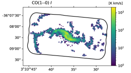
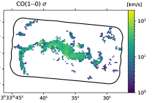
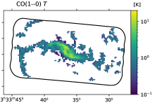
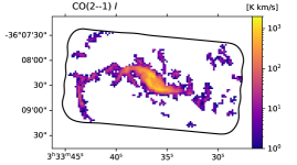
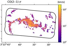
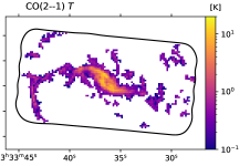
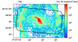
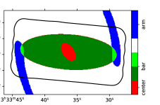
Figure 1: In all panels, the black solid curve represents the CO(2–1) FoV.

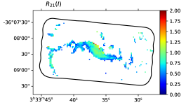
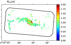
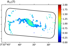
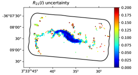
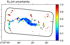
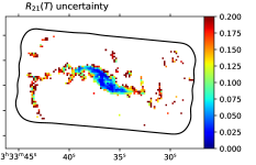
Figure 2: Note that color ranges are different In all panels, the black solid curve represents the CO(2–1) FoV.

3 Results

As seen in the maps of CO(1–0) and CO(2–1) in Figure 1, molecular gas distribution and condition traced by these two transitions are rather similar. Molecular gas is detected in the bar and spiral arms. In the leading edges of the bar, both velocity dispersion ($\sigma$) and peak temperature ($T$) are large, so that the integrated intensity ($I$) and thus the gas column density (which is generally calculated from $I$) are also large. The H$\alpha$ map shows a similar distribution; however, spiral arms appear wider and are easier to trace compared to those in CO maps (at least partially due to a better sensitivity of the H$\alpha$ data).

3.1 CO(1–0) and CO(2–1) (or $R_{21}$)

In Figure 3, correlations between CO(2–1) and CO(1–0) for $I$, $\sigma$, and $T$ are presented. In general, correlations are tight and the ratios are close to unity, which is consistent with the above statement from CO maps – molecular gas distribution and condition traced by CO(1–0) and CO(2–1) are rather similar.

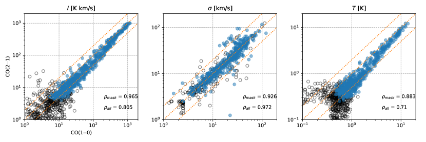
Figure 3: (Left) $I$ of CO(2–1) against that of CO(1–0). Each data point corresponds to a binned pixel with a size of $2^{\prime\prime}$. (Middle) same as the left panel, but for $\sigma$. (Right) same as the left panel, but for $T$.

This non-monotonic behavior is similar to that found in other barred galaxies (e.g., Muraoka et al., 2016; Maeda et al., 2020; Koda et al., 2020). should note that our observations are biased to brighter components and thus to higher ratios. Peñaloza et al. (2017) stated that lower $R_{21}$ comes from a faint area of a GMC, which may not be detected due to the CO sensitivity limit. To discuss azimuthal variation, deeper CO observations are necessary. On the other hand, no clear radial trend of $R_{21}(\sigma)$ is found

In Figure 4, we compare $R_{21}(I)$, $R_{21}(\sigma)$, and $R_{21}(T)$. For the clarity of plots, error bars of $R_{21}(\sigma)$ and $R_{21}(T)$ are omitted. This figure shows majority of data points have $R_{21}(\sigma)$ close to unity, i.e. their line widths are similar for both transitions. For these points, $R_{21}(I)$ is –1.0 and determined by $R_{21}(T)$.

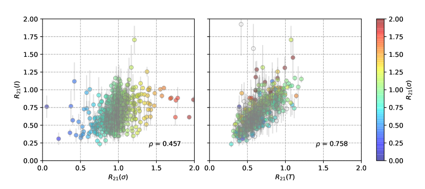
Figure 4: Correlation between the three $R_{21}$ values. $R_{21}(I)$ is plotted against $R_{21}(\sigma)$ (left) and $R_{21}(T)$ (right).

3.2 $R_{21}$ vs H$\alpha$

In Figure 5, three $R_{21}$ values are plotted against the extinction-corrected H$\alpha$ flux (hereafter we just refer it to as “H$\alpha$ flux”). Histograms of these values are added to corresponding axes. Only pixels where both $R_{21}$ and H$\alpha$ are measured are included in these plots. As for Figure 4, error bars of $R_{21}(\sigma)$ and $R_{21}(T)$ are not plotted. From this figure, $R_{21}(I)$ and $R_{21}(T)$ are clearly positively correlated with H$\alpha$ flux , while $R_{21}(\sigma)$ does not depend on H$\alpha$ . While the H$\alpha$ flux increases by $\sim 3.5$ dex, $R_{21}(I)$ and $R_{21}(T)$ increase from $\sim 0.5$ to $\sim 1.0$. This increase is much larger than the prescription by Narayanan & Krumholz (2014). The larger scatter of $R_{21}(I)$ compared to $R_{21}(T)$ is likely due to the large scatter of $R_{21}(\sigma)$.

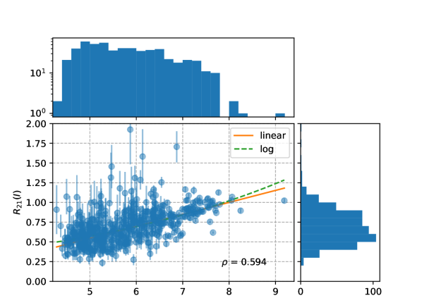
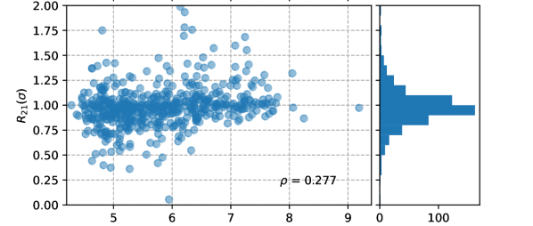
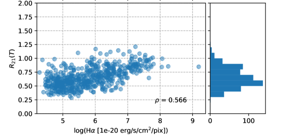
Figure 5: $R_{21}(I)$ (top), $R_{21}(\sigma)$ (middle), and $R_{21}(T)$ (bottom) against log(H$\alpha$). Additional panels on top and right present histograms of H$\alpha$ and corresponding $R_{21}$ values, respectively.

The positive correlation seen in top and bottom panels of Figure 5 is consistent with previous studies and suggests that the ratios are elevated where molecular gas is denser and/or warmer in a close relationship to recent star formation. From our plots and similar plots by Koda et al. (2020); Yajima et al. (2021), we expect a linear relationship between the ratios and log(SFR), Meanwhile, Leroy et al. (2021) described this relationship as a power-law, with an index of $a^{\prime}\simeq 0.13$, where both $R_{21}$ and SFR are normalized by their galactic averages. Maeda et al. (2022) derived similar indices around $\simeq 0.1$ at a 100 pc resolution, with a possible variation among the galactic structures within NGC 1300.

Besides the main positive correlation, we find outliers in three different regions. The first one is $R_{21}(I)>1$ with moderate H$\alpha$ brightness. As already mentioned, these data have large error bars on $R_{21}(I)$ and thus we defer further analysis to a future paper. The third one is the nucleus. While H$\alpha$ is the brightest , $R_{21}(I)$ is just above unity and $R_{21}(T)\simeq 0.85$, both of which are well below the extrapolation of the main correlation . It is likely that the AGN contribution to the H$\alpha$ flux is significant (e.g., Gao et al., 2021) and that the AGN affects surrounding molecular gas in a different way. However, such a significant contribution likely occurs only in this position (i.e., within a single pixel with 200 pc size), as other data points in the bright end do not remarkably deviate from the main correlation.

On the other hand, the dependence of $R_{21}(\sigma)$ on H$\alpha$ brightness is small. This is consistent with our finding in Figure 4 that $R_{21}(\sigma)\simeq 1$ and thus $R_{21}(I)\simeq R_{21}(T)$ for most of the pixels.

4 Discussion

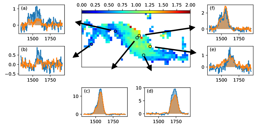
Figure 6: The central panel shows a zoom-in view of $R_{21}(I)$. Subpanels on left present spectra in K for Blue and orange profiles are for CO(1–0) and CO(2–1), respectively. Channels used for moment calculation (i.e., ) are shaded. The selected positions are indicated by open circles on the $R_{21}(I)$ map and connected to the subpanels by arrows. Subpanels on bottom and right are the same as those on left, but for respectively.

Figure 6 presents the selected positions on the $R_{21}(I)$ map and their spectra. The spectra are double peaked or show a second component in most cases, likely due to the complex dynamics explored by Gao et al. (2021) and others. Such multiple components may be in different physical conditions, which can result in different line ratios. we perform spectral fitting with two Gaussian components using CASA specfit. Fitted Gaussians are presented as solid black curves in Figure 7. Fitting with two Gaussians failed for positions (d), and (e) of CO(1–0) spectra, therefore fitting with single Gaussian was performed. Table 1 lists fitting results for each position for each line together with moment values. Difference between $\sigma$ and fitted line width is rather complicated. $\sigma$ becomes larger than of each component (e.g., CO(1–0) (f)). fitted velocity widths are approximately same between CO(1–0) and CO(2–1) except the position (e). This is consistent with our finding based on the moment analysis, i.e. $R_{21}(\sigma)\simeq 1$, and thus both lines trace the same gas components in most cases. Based on these results, if dynamics is simple (i.e., a spectrum has a single component), we claim that $R_{21}(T)$ would be the best indicator of the line ratio especially for faint emission lines.

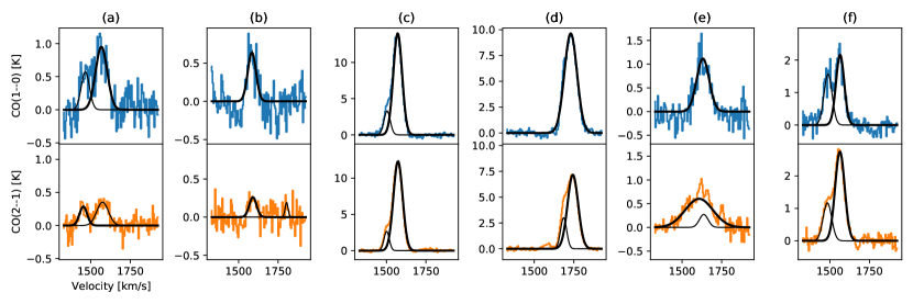
Figure 7: CO(1–0) and CO(2–1) spectra of the selected positions (a)–(f) (same as shown in Figure 6) together with fitted Gaussian profiles (black curves).

Table 1: Properties of selected spectra

Position	Line	Fitting Results														$I$	$\sigma$
		$V_{\rm peak}$		$V_{\sigma}$		$T_{\rm peak}$		$I_{\rm fit}$		$V_{\rm peak}$		$V_{\sigma}$	$T_{\rm peak}$	$I_{\rm fit}$	$\Sigma I_{\rm fit}$
		[km/s]		[km/s]		[K]		[K km/s]		[km/s]		[km/s]	[K]	[K km/s]	[K km/s]	[km/s]	[K km/s]
(a)	CO(1–0)	1567	37	1.0	88	1466	26	0.6	37	125	112 ±5	52
(a)	CO(2–1)	1575	37	0.4	33	1453	24	0.3	17	50	42 ±4	58
(b)	CO(1–0)	1584	26	0.6	42	$\cdots$	$\cdots$	$\cdots$	$\cdots$	42	33 ±3	19
(b)	CO(2–1)	1590	23	0.3	15	1803	9	0.2	5	20	11 ±2	19
(c)	CO(1–0)	1571	28	14.0	978	1504	20	3.3	163	1141	1145 ±5	36
(c)	CO(2–1)	1573	29	12.3	901	1501	17	2.7	112	1013	1012 ±3	37
(d)	CO(1–0)	1730	40	9.6	965	$\cdots$	$\cdots$	$\cdots$	$\cdots$	965	946 ±6	37
(d)	CO(2–1)	1744	34	7.2	603	1686	19	3.0	145	748	746 ±3	39
(e)	CO(1–0)	1632	40	1.1	111	$\cdots$	$\cdots$	$\cdots$	$\cdots$	111	103 ±9	24
(e)	CO(2–1)	1607	88	0.6	132	1637	27	0.3	19	151	132 ±5	65
(f)	CO(1–0)	1565	26	2.2	141	1488	26	1.6	101	242	244 ±6	46
(f)	CO(2–1)	1563	30	2.8	208	1484	27	1.2	79	287	284 ±6	45

Note. — (1) position label. (2) line name. (3)–(6) fitted peak velocity, velocity dispersion, peak temperature, and integrated intensity for the first Gaussian component. (7)–(10) same as (3)–(6) but for the second component. (11) sum of the fitted integrated intensities. (12)–(13) integrated intensity and velocity dispersion from moment calculation with the mask described in §LABEL:sec:mask.

Table 2: Measured ratios for the selected positions

Position	$R_{21}(I)$	$R_{21}(I)_{\rm fit}$
		sum	comp1	comp2
(a)	0.374 ±0.036	0.399	0.371	0.463
(b)	0.350 ±0.080	0.465	0.357	$\cdots$
(c)	0.884 ±0.005	0.887	0.921	0.685
(d)	0.789 ±0.006	0.775	0.625	$\cdots$
(e)	1.286 ±0.122	1.361	1.193	$\cdots$
(f)	1.165 ±0.035	1.185	1.472	0.784

Note. — (1) position label. (2) integrated line ratio from moment 0 values and its uncertainty. (3) integrated line ratio from the sum of $I_{\rm fit}$. (4) integrated line ratio for the first component in Table 1. (5) same as (4) but for the second component if available.

We find that when the fit with two Gaussian components is successful (positions (a), (c), and (f)), The lower ratios suggest that density and/or temperature are lower in such outflowing gas than those in the main disk. difference between the two components highlights the importance of spectral decomposition for accurately measuring the integrated intensity and their ratio in particular when dynamics is complicated.

To obtain a thorough view of the line ratios including their relationship with the gas dynamics, we need to perform spectral fitting in all the pixels. A higher sensitivity will be necessary to discuss line ratios around the bar and in inter-arm regions, while a wider FoV will be necessary to investigate the ratios in the outer disk. Furthermore, quantitatively constraining physical conditions of molecular gas requires data of other lines (e.g. ¹³CO(1–0) as done by Yajima et al. (2021)). We defer these topics to forthcoming papers.

5 Summary

As the ALMA observing efficiency for CO(2–1) emission is better than that for CO(1–0), the former is now popular as a tracer of molecular gas instead of the latter. While their ratio has often been assumed to be constant within and among galaxies, it is naturally expected to be dependent on physical conditions. Here, we report its variation at a $2^{\prime\prime}\simeq 200$ pc resolution in the central $2^{\prime}\times 3^{\prime}$ region of the nearby barred spiral galaxy NGC 1365 using ALMA data. This FoV includes the galactic center, bar, and transition to the spiral arms.

within the FoV is while the scatter is large We also calculate the ratio of velocity dispersions (moment 2) and peak temperatures ($R_{21}(\sigma)$ and $R_{21}(T)$, respectively), and find that $R_{21}(\sigma)\simeq 1$ and thus $R_{21}(I)\simeq R_{21}(T)$ in most cases. This result indicates that both CO(1–0) and CO(2–1) lines generally trace similar components of molecular gas.

We create a map of extinction-corrected H$\alpha$ emission from the data provided by the PHANGS-MUSE project (Emsellem et al., 2021). The $R_{21}(I)$ and $R_{21}(T)$ are found to increase with the H$\alpha$ brightness, which is consistent with recent studies of nearby galaxies but at kpc-scale resolutions (Koda et al., 2020; Yajima et al., 2021; Leroy et al., 2021). We thus conclude that even at 200 pc resolution, $R_{21}(I)$ and $R_{21}(T)$ are elevated where the gas is denser and/or warmer due to recent star formation. Meanwhile, high $R_{21}(I)$ (or $R_{21}(T)$) values with low H$\alpha$ brightness, which are signs of dense but cold molecular gas before star formation, are not

Although the number of positions is small, we find that spectra are often double peaked and that $I$ values (i.e. moment 0) underestimate true integrated intensities when the emissions are weak. Fitting with two Gaussian components works well in most cases and its result supports our conclusion based on the moment calculations. In addition, we identify the second component in spectra of three positions, and find that its integrated intensity ratio is smaller than that of the first component. According to the kinematic model proposed by Gao et al. (2021), these components likely correspond to outflowing gas inside or on the surface of the disk. The smaller ratios suggest that density and/or temperature of this outflowing gas are lower than those in the disk.

References

- Bisbas et al. (2021) Bisbas, T. G., Tan, J. C., & Tanaka, K. E. I. 2021, MNRAS, 502, 2701, doi: 10.1093/mnras/stab121
- Braine & Combes (1992) Braine, J., & Combes, F. 1992, A&A, 264, 433
- Braine et al. (1993) Braine, J., Combes, F., Casoli, F., et al. 1993, A&AS, 97, 887
- Calzetti (2001) Calzetti, D. 2001, PASP, 113, 1449, doi: 10.1086/324269
- den Brok et al. (2021) den Brok, J. S., Chatzigiannakis, D., Bigiel, F., et al. 2021, MNRAS, 504, 3221, doi: 10.1093/mnras/stab859
- Díaz-García et al. (2021) Díaz-García, S., Lisenfeld, U., Pérez, I., et al. 2021, A&A, 654, A135, doi: 10.1051/0004-6361/202140674
- Druard et al. (2014) Druard, C., Braine, J., Schuster, K. F., et al. 2014, A&A, 567, A118, doi: 10.1051/0004-6361/201423682
- Emsellem et al. (2021) Emsellem, E., Schinnerer, E., Santoro, F., et al. 2021, arXiv e-prints, arXiv:2110.03708. https://arxiv.org/abs/2110.03708
- Fazeli et al. (2019) Fazeli, N., Busch, G., Valencia-S., M., et al. 2019, A&A, 622, A128, doi: 10.1051/0004-6361/201834255
- Gao et al. (2021) Gao, Y., Egusa, F., Liu, G., et al. 2021, ApJ, 913, 139, doi: 10.3847/1538-4357/abf738
- Gong et al. (2020) Gong, M., Ostriker, E. C., Kim, C.-G., & Kim, J.-G. 2020, ApJ, 903, 142, doi: 10.3847/1538-4357/abbdab
- Herrera et al. (2020) Herrera, C. N., Pety, J., Hughes, A., et al. 2020, A&A, 634, A121, doi: 10.1051/0004-6361/201936060
- Jang et al. (2018) Jang, I. S., Hatt, D., Beaton, R. L., et al. 2018, ApJ, 852, 60, doi: 10.3847/1538-4357/aa9d92
- Jorsater & van Moorsel (1995) Jorsater, S., & van Moorsel, G. A. 1995, AJ, 110, 2037, doi: 10.1086/117668
- Kepley et al. (2020) Kepley, A. A., Tsutsumi, T., Brogan, C. L., et al. 2020, PASP, 132, 024505, doi: 10.1088/1538-3873/ab5e14
- Koda et al. (2019) Koda, J., Teuben, P., Sawada, T., Plunkett, A., & Fomalont, E. 2019, PASP, 131, 054505, doi: 10.1088/1538-3873/ab047e
- Koda et al. (2012a) Koda, J., Yagi, M., Boissier, S., et al. 2012a, ApJ, 749, 20, doi: 10.1088/0004-637X/749/1/20
- Koda et al. (2012b) Koda, J., Scoville, N., Hasegawa, T., et al. 2012b, ApJ, 761, 41, doi: 10.1088/0004-637X/761/1/41
- Koda et al. (2020) Koda, J., Sawada, T., Sakamoto, K., et al. 2020, ApJ, 890, L10, doi: 10.3847/2041-8213/ab70b7
- Leroy et al. (2021) Leroy, A. K., Rosolowsky, E., Usero, A., et al. 2021, arXiv e-prints, arXiv:2109.11583. https://arxiv.org/abs/2109.11583
- Lindblad (1999) Lindblad, P. O. 1999, A&A Rev., 9, 221, doi: 10.1007/s001590050018
- Maeda et al. (2022) Maeda, F., Egusa, F., Ohta, K., et al. 2022, ApJ, 926, 96, doi: 10.3847/1538-4357/ac4505
- Maeda et al. (2020) Maeda, F., Ohta, K., Fujimoto, Y., Habe, A., & Ushio, K. 2020, MNRAS, 495, 3840, doi: 10.1093/mnras/staa1296
- Mangum & Shirley (2015) Mangum, J. G., & Shirley, Y. L. 2015, PASP, 127, 266, doi: 10.1086/680323
- McMullin et al. (2007) McMullin, J. P., Waters, B., Schiebel, D., Young, W., & Golap, K. 2007, in Astronomical Society of the Pacific Conference Series, Vol. 376, Astronomical Data Analysis Software and Systems XVI, ed. R. A. Shaw, F. Hill, & D. J. Bell, 127
- Muraoka et al. (2016) Muraoka, K., Sorai, K., Kuno, N., et al. 2016, PASJ, 68, 89, doi: 10.1093/pasj/psw080
- Narayanan & Krumholz (2014) Narayanan, D., & Krumholz, M. R. 2014, MNRAS, 442, 1411, doi: 10.1093/mnras/stu834
- Nishimura et al. (2015) Nishimura, A., Tokuda, K., Kimura, K., et al. 2015, ApJS, 216, 18, doi: 10.1088/0067-0049/216/1/18
- Peñaloza et al. (2018) Peñaloza, C. H., Clark, P. C., Glover, S. C. O., & Klessen, R. S. 2018, MNRAS, 475, 1508, doi: 10.1093/mnras/stx3263
- Peñaloza et al. (2017) Peñaloza, C. H., Clark, P. C., Glover, S. C. O., Shetty, R., & Klessen, R. S. 2017, MNRAS, 465, 2277, doi: 10.1093/mnras/stw2892
- Querejeta et al. (2021) Querejeta, M., Schinnerer, E., Meidt, S., et al. 2021, arXiv e-prints, arXiv:2109.04491. https://arxiv.org/abs/2109.04491
- Rosolowsky & Leroy (2006) Rosolowsky, E., & Leroy, A. 2006, PASP, 118, 590, doi: 10.1086/502982
- Saintonge et al. (2017) Saintonge, A., Catinella, B., Tacconi, L. J., et al. 2017, ApJS, 233, 22, doi: 10.3847/1538-4365/aa97e0
- Sakamoto et al. (2007) Sakamoto, K., Ho, P. T. P., Mao, R.-Q., Matsushita, S., & Peck, A. B. 2007, ApJ, 654, 782, doi: 10.1086/509775
- Sandqvist et al. (1995) Sandqvist, A., Joersaeter, S., & Lindblad, P. O. 1995, A&A, 295, 585
- Sawada et al. (2001) Sawada, T., Hasegawa, T., Handa, T., et al. 2001, ApJS, 136, 189, doi: 10.1086/321793
- Sorai et al. (2001) Sorai, K., Hasegawa, T., Booth, R. S., et al. 2001, ApJ, 551, 794, doi: 10.1086/320212
- Sun et al. (2018) Sun, J., Leroy, A. K., Schruba, A., et al. 2018, ApJ, 860, 172, doi: 10.3847/1538-4357/aac326
- van der Tak et al. (2007) van der Tak, F. F. S., Black, J. H., Schöier, F. L., Jansen, D. J., & van Dishoeck, E. F. 2007, A&A, 468, 627, doi: 10.1051/0004-6361:20066820
- Véron-Cetty & Véron (2010) Véron-Cetty, M. P., & Véron, P. 2010, A&A, 518, A10, doi: 10.1051/0004-6361/201014188
- Yajima et al. (2021) Yajima, Y., Sorai, K., Miyamoto, Y., et al. 2021, PASJ, 73, 257, doi: 10.1093/pasj/psaa119
- Yoda et al. (2010) Yoda, T., Handa, T., Kohno, K., et al. 2010, PASJ, 62, 1277, doi: 10.1093/pasj/62.5.1277
- Zschaechner et al. (2018) Zschaechner, L. K., Bolatto, A. D., Walter, F., et al. 2018, ApJ, 867, 111, doi: 10.3847/1538-4357/aadf32