Neural Topological Ordering for Computation Graphs

Abstract

Recent works on machine learning for combinatorial optimization have shown that learning based approaches can outperform heuristic methods in terms of speed and performance. In this paper, we consider the problem of finding an optimal topological order on a directed acyclic graph with focus on the memory minimization problem which arises in compilers. We propose an end-to-end machine learning based approach for topological ordering using an encoder-decoder framework. Our encoder is a novel attention based graph neural network architecture called Topoformer which uses different topological transforms of a DAG for message passing. The node embeddings produced by the encoder are converted into node priorities which are used by the decoder to generate a probability distribution over topological orders. We train our model on a dataset of synthetically generated graphs called layered graphs. We show that our model outperforms, or is on-par, with several topological ordering baselines while being significantly faster on synthetic graphs with up to 2k nodes. We also train and test our model on a set of real-world computation graphs, showing performance improvements.

1 Introduction

Many problems in computer science amount to finding the best sequence of objects consistent with some precedence constraints. An intuitive example comes from routing problems, where we would like to find the shortest route between cities but we have requirements (i.e. for example to pick up and subsequently deliver a package) on the order in which the cities should be visited [1]. Another case is found in compiler pipelines, wherein the "cities" become operations to be executed and the constraints come from the data dependencies between these operations, such as when the result of an operation is an operand in a subsequent one. In this case, the metric to be optimized can be the run time of the compiled program, or the memory required to execute the program [2]. Common across this class of problems is their formulation in term of finding the optimal topological order of the Directed Acyclic Graph (DAG) that encodes the precedence constraints, which induces a Combinatorial Optimization [3] (CO) problem which is in general computationally hard [4].

Already from the two examples above, one can immediately grasp the relevance of such problems for industrial Operations Research, which has prompted various actors to invest in the development of efficient CO solvers; these solvers usually encapsulate heuristic methods whose design typically requires extensive use of domain-specific and problem-specific knowledge, across decades of development. In recent years, considerable interest has emerged in the possibility of replacing such handcrafted heuristics with ones learned by deep neural nets [5] (machine learning for combinatorial optimization, MLCO). As a matter of fact, both of our two examples of DAG-based CO problems have indirectly been object of study in the Machine Learning literature. References [6, 7, 8, 9] take into consideration Routing Problems, especially the Traveling Salesperson Problem (TSP) which, on account of its richness, complexity and long history of mathematical study [10], has attained the status of a standard benchmark for MLCO [8]. Conversely, less attention has been devoted to operations sequencing likely due to the proprietary and sensitive nature of compiler workflows, which hampers the definition of public benchmarks. References [11, 12] both consider the task of optimizing the run time of a neural network’s forward pass by optimizing the ordering and device assignment of its required operations. However, in this last case the sequencing stage is only one part of a larger compiler pipeline, and as a result of this both the performance metrics and the datasets employed cannot be made available for reproduction by third parties. This makes it both hard to assess the results therein, and to draw general conclusions and guidelines for the advancement of MLCO, which still suffers from a lack of commonly accepted and standard datasets and benchmarks.

In this work, we address the problem of finding optimal topological orders in a DAG using deep learning, focusing on the compiler task of optimizing the peak local memory usage during execution. We make the following contributions:

• We present a neural framework to optimize sequences on directed acyclic graphs. Mindful of the need for scalability, we consider a non-auto-regressive (NAR) scheme for parametrizing the probability distribution of topological orders. This allows our method to attain an extremely favorable performance vs. run time tradeoff: it always outperforms fast baselines, and is only matched or outperformed by those requiring a much longer (in one case 4000x more) run time.

• We address the problem of how to perform meaningful message-passing on DAGs, a graph type which has received comparatively less attention in the literature on Graph Neural Networks. We introduce Topoformer, a flexible, attention-based architecture wherein messages can be passed between each and every pair of nodes, with a different set of learnable parameters depending on the topological relation between the nodes.

• To test our method, we introduce an algorithm for the generation of synthetic, layered, Neural Net-like computation graphs, allowing any researcher to generate a dataset of as many as desired graphs of any desired size. These graphs are a more faithful model of real NN workflows, and allow us to prove our method on a much larger and varied dataset, than previous efforts [11]. To our knowledge, this is the first public algorithm of this kind. Nevertheless, we also test our method on proprietary graphs to illustrate its relevance to realistic compiler workflows.

2 Related work

Machine Learning for Combinatorial Optimization:

Combinatorial optimization as a use case for deep learning poses interesting technical challenges. First, the combinatorial nature of the problem conflicts with the differentiable structure of modern deep neural networks; and second, the models need to be run at large scale to solve real world instances, exacerbating the challenges in training deep learning models. Given the discrete nature of CO problems, a natural approach is to pose them as reinforcement learning (RL) problems [13]. The aim is then to learn a policy that selects the best actions to maximize a reward directly related to the optimization objective. Algorithms then differ in the way the policy is parameterized: either in an end-to-end manner where the actions directly correspond to solutions of the optimization problem [12, 6, 8, 14], or in a hybrid manner, where the policy augments parts of a traditional solver, e.g. by replacing heuristics used in setting parameters of an algorithm, see e.g. [11, 9, 7, 2]. Our approach follows an end-to-end design philosophy, which, not having to rely on an external algorithm, affords better control of post-compile run time and facilitates application on edge devices [2]. Furthermore, RL has the advantage of being useful as a black box optimizer, when no handcrafted heuristics can be designed.
Sequence Optimization via ML: Within MLCO, much effort has been devoted to the task of predicting optimal sequences [15, 6, 16, 17, 18]. The end-to-end nature of our method places it close to the one proposed in [6], although to the best of our knowledge, our work is the first to tackle the challenge of enforcing precedence constraints in the network predictions. As we shall see in more detail below, this generalization is non-trivial: already counting the number of topological orders belongs to the hardest class of computational problems [4]. This has to be contrasted with the fact that the number of sequences without topological constraints is simply $n!$ for $n$ objects. Besides, as pointed out in [8], no MLCO method has so far been able to convincingly tackle TSPs of sizes above a few hundred nodes, when it comes to zero-shot generalization to unseen problem instances, i.e. when no fine tuning on the test set is done. It is also therein pointed out how an auto-regressive parametrization of the sequence (which was the method used in ref. [6]) appears to be necessary to achieve acceptable performance even at those small sizes. Conversely, in the present work we show compelling zero-shot performance on DAGs of sizes up to thousands of nodes, while nonetheless generating our sequences in a fully non-auto-regressive (NAR) way and maintaining a strong run time advantage over classical sequencing algorithms. Our results can then also be interpreted as cautioning against the idea of using the TSP as the sole, paradigmatic test-bed for MLCO research, as [8] remarks.
ML for Compiler Optimization: The DAG sequencing task we consider is an omnipresent stage in compiler workflows, which usually also include such tasks as device assignment and operations fusion [12]. In such a setting, jointly optimizing these tasks to reduce the run time of a certain workflow (such as the forward pass of a Neural Net) is a common objective, which in refs [11, 12, 19] is tackled with ML methods. In this work we focus on the task of minimizing the peak local memory usage during execution, which does not require a performance model or simulator as well as being relevant to applications on edge devices [2]. In  [11], the ML solution leans on an existing genetic algorithm, whilst our solution is end-to-end, much like that proposed in  [12]. Another characteristic of the solution proposed in [12] is the idea of interpolating between AR and NAR via an iterative refinement scheme, in which sequences are generated in one pass but subsequently refined during an user-defined number of subsequent passes; conversely, we generate all our sequences in a single pass.
While in [11] the run time optimization is studied on both real-world and synthetic random graphs – the latter being relatively small (up to about 200 nodes), the peak memory optimization is studied only on a proprietary dataset augmented via perturbation of the node attributes. In [12] the authors train and test their method on a relatively small set of six proprietary workflows which are not disclosed to the reader, and out of those six, only the size of the largest instance is mentioned.
Deep Graph Neural Networks: Given that our problem is specified as a DAG, it is a logical choice to parametrize our sequence-generation policy with a Graph Neural Network architecture [20]. The basic idea of every GNN architecture is to update graph and edge representations by passing messages between the graph nodes along the graph edges [21]. However, this can be too restrictive when it comes to sequence generation on DAGs. For example, nodes that come after each other in the sequence might not be linked by an edge in the graph, and therefore are unable to directly influence each other’s representation. Notice how this difficulty is another consequence of the presence of precedence constraints in our problem, which conversely was not an issue in e.g. [6] where the graph is fully connected and no constraints are present. Relatively few efforts (see e.g. [22, 23, 24]) have been devoted to devise a way to perform meaningful message passing on DAGs. As a matter of fact, the quest for expressive GNN architectures is at the center of intense theoretical investigation [25, 26].

3 Background

3.1 Topological Orders and DAGs

We here introduce the mathematical background, starting with a few definitions. A partial order is an irreflexive transitive relation $<$ between certain pairs of a set $V$. We call a pair $(x,y)\in V\times V$ that is related by $<$ comparable, and incomparable otherwise. A Directed Acyclic Graph (DAG) $G=(V,E)$ is a directed graph with no directed loops. We can map a DAG $G=(V,E)$ to a partially ordered set $(V,<)$ where $x<y$ if there is a directed path from node $x$ to node $y$. Multiple DAGs map to the same partial order. For example, the DAGs with vertex set $\{x,y,z\}$ and edge sets $E=\{x\to y,y\to z\}$ and $E^{\prime}=\{x\to y,y\to z,x\to z\}$, where $s\to t$ denotes a directed edge from $s$ to $t$, correspond to the same partial order $x<y<z$. We define the transitive closure (TC) of a DAG as the graph with most edges that has the same underlying partial order, so that there exists a directed edge $(x,y)$ whenever $x<y$. Conversely, the transitive reduction (TR) is the graph with least edges that results in the same partial order. We denote the order induced by a DAG by $<_{G}$.

A topological order or sorting of a DAG $G$ is a bijection $\sigma:V\to\{1,\dots,|V|\}$ such that $\sigma(x)<\sigma(y)$ whenever $x<_{G}y$. The set ${\cal T}_{G}$ of topological orders of $G$ is a subset of the permutation group of the vertices and coincides with total orders on $V$ that respect $<_{G}$, called linear extensions of the partial order. While there are several well-known algorithms to compute a topological order of a DAG, e.g. breadth first search and depth first search, counting the number of topological orders is one of the hardest computational problems, being $\#$P complete [4]. In this work we develop a general machine learning method to find a topological order that minimizes a given cost function on a DAG, which we define in the next section.

3.2 Peak Memory Minimization

Deciding the best way to schedule operations in a computational graph representing a neural network is a central problem in compilers [11, 12, 2]. We can associate a DAG to a computational graph in such a way that nodes represent operations ("ops"), and incoming/outgoing edges represent operands/results of these operations. Every time one executes an op, the inputs to that op need to be in memory, and memory for the outputs needs to be allocated. Therefore, each node of the DAG carries a label $m:V\to\mathbb{N}$ specifying the memory required to store the output of that op. A typical first step in scheduling a DAG is to identify topological orders to execute operations. Compilers for edge devices, which have limited memory, aim at choosing the optimal topological order that minimizes the peak memory footprint [2]. We focus therefore on the peak local memory usage minimization task, which can be formulated as the following combinatorial optimization problem on a labeled DAG $G=(V,E,m)$:

$$\min_{\sigma\in{\cal T}_{G}}\mathcal{C}(\sigma),\qquad\mathcal{C}(\sigma)=\max(M_{1}(\sigma),\dots,M_{|V|}(\sigma)),$$ (1)

with the definitions

$$M_{t} =I_{t-1}+m(\sigma_{t}),$$ (2)

$$I_{t} =M_{t}-\sum_{i\in S_{t}}m_{i},\qquad S_{t}=\left\{i:i\notin\bigcup_{l=0}^{t-1}S_{l}~{}~{}\text{ and }~{}~{}\forall(i,j)\in E,\,j\in\sigma_{1:t}\right\},$$ (3)

i.e. the memory usage at time $t$ is given by the memory usage $I_{t-1}$ of the outputs which have not yet been consumed, at time $t-1$, by downstream operations, plus the memory requirement of the output of operation $\sigma(t)$. $I_{t}$ is in turn obtained by subtracting from $M_{t}$ the memory costs of nodes whose outgoing edges only connect to already scheduled nodes, i.e. nodes whose output was only required by already scheduled operations. Naturally, $I_{0}=0,S_{0}=\phi$.

4 Method

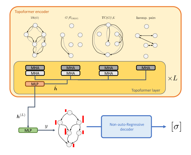
Figure 1: Our complete architecture for neural topological ordering. The shades of gray in the MHA boxes are to highlight how attentions heads operate separately on the forward and backward version of the first three graphs. The priorities $(y_{i})_{i=1}^{|V|}$ are represented by the red bars on the original DAG and decoded into a sequence with its associated probability.

We use an encoder-decoder architecture whose schematic is shown in figure 1. Our encoder is Topoformer, a novel GNN architecture, which derives an embedding for each node of the graph. The embeddings are used by the decoder which generates a distribution in the sequence space and finally the distribution can be converted to a sequence via different inference methods like sampling, greedy inference or beam search. Next, we describe each of the component in detail.

4.1 Topoformer: Topologically Masked Attention

A Graph Neural Network (GNN) is a natural choice to encode our scheduling problem via embedding of the DAG nodes. All canonical GNN architectures operate by updating these embeddings via the aggregation of "messages" sent from the other nodes, usually in the form of some function of their own embedding [20]. Architectures mainly differ in how the set of sender nodes is constructed and the aggregation function is chosen. In a Graph Convolutional Network [27], the senders are the first neighbors of a node and the aggregation function is a weighted average, whilst in a vanilla Graph Attention Network [28], the senders are all the other nodes, but their contributions are aggregated via averaging with learned weights so as to account for their degree of relevance. When trying to apply such mechanisms on DAGs, a common point of contention is whether, and how in practice, the partial ordering encoded by it should reflect in the direction of travel of the messages [29, 24, 22]. While disregarding the DAG structure entirely (as one would do in a vanilla GAT), does not appear wise, it might be too restrictive when it comes to our task. For example, nodes that are next to each other in the sequence might well be incomparable, and thus lack a path for messages between them. The combinatorial nature of the task also poses requirements; it is known [25, 5] that reasoning about CO problems on a graph requires the capacity to reason about the global structure of it, whilst architectures such as those proposed in [29, 24, 22] limit the set of sender nodes to a local neighborhood of the receiver node. In summary, our architecture must strike a compromise between accounting for global structure and local partial ordering information.

Our Topoformer architecture meets these requirements. A vector $\boldsymbol{x}_{i}$ of input features (see the appendix for details about its definition and dimensionality) is first turned into an initial node embedding $\boldsymbol{h}_{i}^{(0)}$ via a node-wise linear transformation, $\boldsymbol{h}_{i}^{(0)}=W\boldsymbol{x}_{i}+\boldsymbol{b}$. Subsequently, a succession of $L$ attention layers, each of them consisting of a Multi-Head Attention (MHA) [28] sub-layer followed by one more node-wise MLP, updates these embeddings, similar to a vanilla Transformer [30]; however, we confer a topological inductive bias to these updates by having a separate group of attention heads masked by each of the following graphs induced by the original DAG:

• Its transitive reduction (TR).

• The directed graph obtained by removing the TR edges from the DAG: $G\backslash E_{\textrm{TR}(G)}$.

• The directed graph obtained by removing the edges of the DAG from its TC: $\textrm{TC}(G)\backslash E$.

• The backwards versions (i.e. with flipped edges) of each of the three above.

• The undirected graph obtained by joining all incomparable node pairs.

By adding together these graphs, one would obtain the fully connected graph relative to the node set $V$, whereupon all nodes would attend to all nodes. Then effectively, the propagation rules of Topoformer are same as those of a vanilla transformer encoder,

$$\hat{\boldsymbol{h}}_{i}^{(\ell)}= \boldsymbol{h}_{i}^{(\ell-1)}+\texttt{concat}_{j}\left[\textrm{MHA}_{i}^{\ell,j}\left(\boldsymbol{h}_{1}^{(\ell-1)},\dots,\boldsymbol{h}_{|V|}^{(\ell-1)};M^{j}\right)\right],$$ (4)

$$\boldsymbol{h}^{(\ell)}_{i}= \hat{\boldsymbol{h}}_{i}^{(\ell)}+\textrm{MLP}^{(\ell)}\left(\hat{\boldsymbol{h}}_{i}^{(\ell)}\right),$$ (5)

save for the presence of the mask $M^{j}$, which ensures that head $j$ only attends to its assigned graph among the seven listed above. Following [31], we also apply layer normalization [32] to the MHA and MLP inputs. The number of heads assigned to each graph can be chosen independently (setting it to zero means to not message-pass along the edges of the respective graph), or parameters can be tied among different MHAs. One should also remark how the MLP sub-layer allows the flow of information between different attention heads. All nodes are then able to influence each other’s representation, while anyway injecting a strong inductive bias based on the DAG structure. Information about the Topoformer configurations used in our experiments is provided in the appendix.

4.2 Decoder

Once the embeddings of the nodes are generated, the decoder’s task is to derive a stochastic policy $p(\sigma|G)$ over the valid topological orders of the graph. The most straightforward way is to take advantage of the chain rule of conditional probability to decompose the policy as a product

$$p(\sigma|G)=\prod_{t=2}^{|V|}p_{\theta}(\sigma_{t}|\sigma_{1:t-1},\boldsymbol{h},G)\times p_{\theta}(\sigma_{1}|\boldsymbol{h},G),$$ (6)

We could then sample a complete sequence by autoregressively choosing a new node at each step as done e.g. in [6]. This scheme is the most principled and expressive; however, when a NN is used as a function approximator for $p_{\theta}$, it also requires that $|V|$ calls to this NN be performed, which limits its feasibility to relatively small graphs due to the amount of computation required.

In order to scale to large graphs, we employ a Non-Auto-Regressive (NAR) scheme which decouples the number of NN calls from the graph size. Similar to the approach of [12], we assign scheduling priorities $y_{i}\in\mathbb{R}$ to the nodes, rather than scheduling probabilities. The priority for node $i$ is derived by passing its final embedding through an MLP:

$$y_{i}=\textrm{MLP}\left(\boldsymbol{h}^{(L)}_{i}\right).$$ (7)

These priorities are assigned with a single NN inference. The sequence itself is subsequently constructed by adding a new node at each step. Given the partial sequence $\sigma_{1:i-1}$, the next node can only be selected from a subset $\mathcal{S}(\sigma_{1:i-1},G)$ of schedulable nodes, due to both the graph topology and choices made earlier in the sequence. Then, the distribution of the next node to be added at step $i$ is given as follows:

$$p(\sigma_{t}|\sigma_{1:t-1},\boldsymbol{h},G)=\begin{cases}\dfrac{\exp(y_{\sigma_{t}})}{\sum_{j\in\mathcal{S}(\sigma_{1:t-1},G)}\exp(y_{j})},~{}~{}&\text{if }\sigma_{t}\in\mathcal{S}(\sigma_{1:t-1},G),\\ 0,~{}~{}~{}&\text{otherwise.}\end{cases}$$ (8)

Decoding Methods: We use the following three methods to obtain the next node in the partial sequence from the distribution $p(\sigma_{t}|\sigma_{1:t-1},\boldsymbol{h},G)$:

1. Greedy: At each step $t$, select the node with the highest probability i.e. $\sigma_{t}=\operatorname*{arg\,max}_{\tilde{\sigma}_{t}}p(\tilde{\sigma}_{t}|\sigma_{1:t-1},\boldsymbol{h},G)$

2. Sampling: At each step $t$, sample from the next node distribution i.e. $\sigma_{t}\sim p(\cdot|\sigma_{1:t-1},\boldsymbol{h},G)$

3. Beam search with state-collapsing: We can also expand the partial sequences by using a beam search method where the score function is total probability of the partial sequence. We improve our beam search routine by making the following observation: suppose there are two partial sequences in consideration, $\sigma_{1:t}$ and $\tilde{\sigma}_{1:t}$, such that both have scheduled the same set of nodes so far (but different order), and $\mathcal{C}(\sigma_{1:t})<\mathcal{C}(\tilde{\sigma}_{1:t})$. Then, we can ignore the partial sequence $\tilde{\sigma}_{1:t}$ and only keep $\sigma_{1:t}$ in the beam search. This is because both partial sequences must schedule the same set of remaining nodes, and hence the set of future memory costs are identical for both $\sigma_{1:t}$ and $\tilde{\sigma}_{1:t}$, but the current peak memory cost is higher for $\tilde{\sigma}_{1:t}$. Thus, $\sigma_{1:t}$ dominates $\tilde{\sigma}_{1:t}$ in terms of achievable minimal peak memory usage.

4.3 Training

Our encoder-decoder architecture induces a distribution $p_{\theta}(\sigma|G)$ on the set of topological orders for a given DAG $G$. The expected cost incurred is given by $J(\theta|G)=\mathbb{E}_{p_{\theta}(\sigma|G)}\left[\mathcal{C}(\sigma(\theta))\right]$. We minimize the cost $J(\theta)=\mathbb{E}_{G}\left[J(\theta|G)\right]$ via gradient descent using the REINFORCE gradient estimator  [33, 13] as follows

$$\nabla J(\theta)=\mathbb{E}_{G,p_{\theta}(\sigma|G)}\left[(\mathcal{C}(\sigma)-b(G)\right)\nabla_{\theta}\log p_{\theta}(\sigma|G)],$$ (9)

where $b(G)$ is a baseline meant to reduce the variance of the estimator. We follow [6] in setting it equal to the cost of a greedy rollout of a baseline policy on the graph $G$

$$b(G)=\mathcal{C}(\operatorname*{arg\,max}_{\sigma}p_{\theta}(\sigma|G)).$$ (10)

5 Experiments

We conduct experiments on a synthetic dataset of graphs which we refer to as "layered graphs", as well as a set of real-world computation graphs. We compare our approach with the following classic topological ordering baselines:

• Depth/Breadth first sequencing: Find the topological order by traversing the graph in depth/breadth first manner according to the layout of the graph generated using pygraphviz.

• Depth-first dynamic programming (DP): Depth-first DP is a global depth-first method for searching the optimal sequence, with automatic backtracking when equivalent partial sequences are found; it retains the full sequence with minimum cost so far, and returns it if search does not complete before the prescribed timeout.

• Approximate DP: In approximate DP, a beam of partial sequences are considered at each step. For each beam in the subsequent step, the top-$K$ partial sequences with the lowest costs are retained. This DP is also able to find the optimal sequence given enough memory and compute resources (with unlimited beam size $K$), but we only consider an approximate version with $K=10^{5}$ in this work. Note that approximate DP uses the state-collapsing and parallelism to improve its efficiency.

• Random order: We generate $100$ random topological orders, and pick the one with smallest cost.

Please see the appendix for more detailed description of the baselines. Therein, we also report some ablation studies on various neural baselines including ablation studies on decoder by considering other neural architectures, as well as a comparison with an end to end baseline adapted from ref. [6]. Neural topo order greedy, sample and BS denote the performance of our model in greedy, sampling and beam search inference mode respectively. We use a sample size and beam size of $16$ sequences, of which the best one is subsequently picked, for all our experiments. Next, we describe in detail the results of the two experiments.

5.1 Layered Graphs

In order to generate a large corpus of training data we come up with a way to synthetically generate graphs of a given size which have similar structure to the computation graphs of feed-forward neural networks. We call our synthetic graph family layered graphs, as these graphs comprise of well-defined layers of nodes. The nodes in a layer have connections to the nodes in the subsequent layer and can also have skip connections with nodes in layers farther down. The number of layers, number of node per layer, number of edges between subsequent layers, number of skip connections and memory utilization of the nodes are all generated randomly, and can be controlled by setting appropriate parameters. We refer the reader to the appendix for more details on layered graphs, including their generation algorithm and some visual examples.

We train our model on $500$-node layered graphs for $325$ epochs, where in each epoch we generate a training set of $1000$ new graphs. We test the performance of our model on a set of 300 unseen graphs of the same size, generated with the same method. We also evaluate the cross-size generalization performance of our trained model by testing it on graphs of size $1000$ and $2000$. We refer the reader to the appendix for a comprehensive description of the training algorithm and model configuration.

Figure 2 shows the performance vs. run time plot on layered graphs of size $|V|=500,1000$, and $2000$. We report the performance in terms of the % gap of peak memory utilization from the peak memory obtained via approximate DP, which we consistently observed to be the best-performing baseline. Note that the run time is plotted on a log-scale. We can observe that for $500$-node graphs, our model beats all the baselines except approximate DP in terms of both the memory usage and run time. Our model is slightly worse than approximate DP from the memory usage perspective, but it runs 100x faster. We also observe that our model generalizes well to larger sized graphs. For the case of $2000$-node graphs our model performs better than approximate DP in terms of peak memory usage, while being $4000$x times faster. This shows that while approximate DP performs more poorly as graph size increases, our model is able to generalize to larger graphs by learning meaningful embeddings of the topological structure thanks to Topoformer, and to be extremely fast thanks to our NAR decoding scheme.

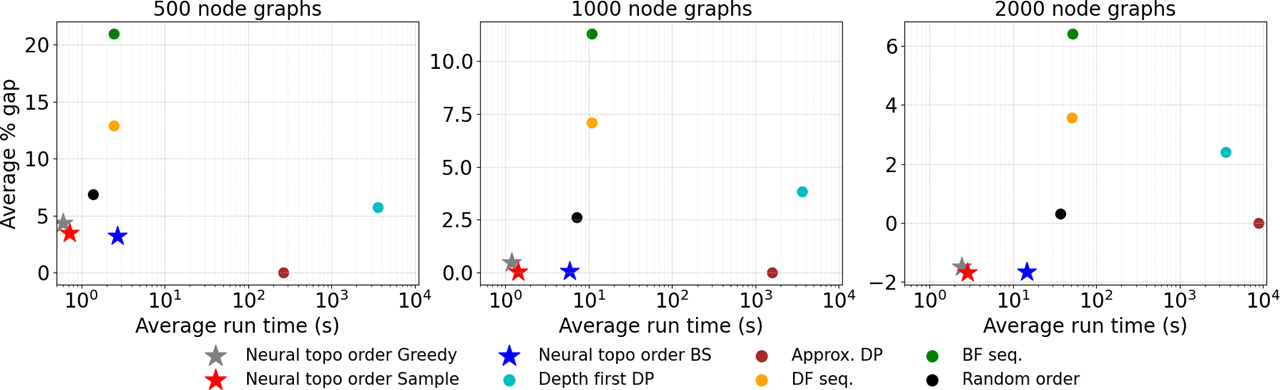
Figure 2: Average % gap from approximate DP vs average run time comparison on the test set of 300 layered graphs. Lower is better for both % gap and run time.

Table 1: Comparison of methods on the synthetic layered graph test set.

Algorithm	500- node graphs		1000-node graphs		2000-node graphs
	% gap from	run time	% gap from	run time	% gap from	run time
	approx. DP	[$s$]	approx. DP	[$s$]	approx. DP	[$s$]
Approximated DP	0	264.88	0	1561.17	0	8828.86
Depth-First DP	5.76	3600	3.84	3600	2.40	3600
(max. run time=1H)
Random order	6.86	1.38	2.62	7.13	0.31	36.87
Depth-first seq.	12.9	2.45	7.1	10.91	3.57	51.32
Breadth-first seq.	20.94	2.43	11.31	10.87	6.42	51.52
Neural Topo Order
✓Greedy	4.32	0.6	0.48	1.19	-1.47	2.44
✓Sample	3.49	0.72	0.03	1.41	-1.68	2.87
✓Beam search	3.21	2.68	0.08	5.92	-1.66	14.74

5.2 Real-World Graphs

While our synthetic layered graphs are convenient for experimentation, we see value in also presenting results obtained from neural computation graphs used for commercial development of our artificial intelligence hardware and software products. Here we sample 115 representative graphs that have diverse architectures (classifiers, language processors, denoisers, etc.) and size (from a few dozen to 1k nodes). We split this dataset into a training set and test set via a random $80-20$ split. We train our model for $500$ epochs and report the performance on the unseen test set at the end of training in table 2. In order to ensure fair comparison of run times, we stratify the test set into 3 categories based on the graph size. Figure 3 shows the performance vs run time plot on the test set of real graphs. We observe that for real graphs the performance gap between the best baseline (approximate DP) and our model is remarkable. We can obtain sequences which are $50\%$ better than approximate DP on average while also being almost 1000x faster on average. This proves the capability of our model to generalize and perform well on real-world computation workflows.

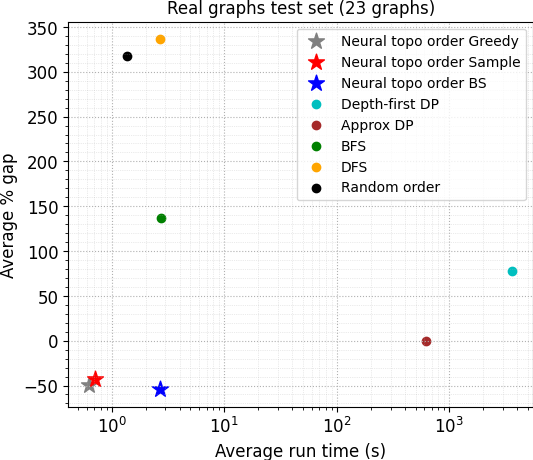
Figure 3: Performance vs run time comparison for different approaches on test set of real computation graphs. Performance is measured in average % gap from approximate DP.

Table 2: Comparison of methods on the real graph test set. Smaller % gap is better

Algorithm	200 - 500-node graphs		500 - 700-node graphs		700 - 1000-node graphs
	% gap from	run time	% gap from	run time	% gap from	run time
	approx. DP	[$s$]	approx. DP	[$s$]	approx. DP	[$s$]
Approximated DP	0	113.54	0	517.60	0	1131.61
Depth-First DP	62.18	3600	102.76	3600	50.57	3600
(max. run time=1H)
Random order	469.34	0.25	376.16	1.24	116.24	2.40
Depth-first seq.	506.21	0.70	394.93	2.26	123.21	4.49
Breadth-first seq.	348.77	0.75	149.81	2.31	-35.55	4.86
Neural Topo Order
✓Greedy	-17.57	0.42	-51.23	0.6	-68.97	0.83
✓Sample	-21.53	0.44	-40.51	0.68	-61.46	0.97
✓Beam search	-19.5	1.22	-57.34	2.58	-73.45	3.86

5.3 Encoder Ablation Study

Table 3: Comparison of different encoder architectures. Topoformer with MP (message passing) on DAG corresponds to forward and backward message passing only on the input DAG using topoformer.

Algorithm	500-node graphs		1000-node graphs
	% gap from	run time	% gap from	run time
	approx. DP	[$s$]	approx. DP	[$s$]
MLP
✓Greedy	8.31 $\pm$ 0.76	0.58 $\pm$ 0.0	2.95 $\pm$ 0.48	1.52 $\pm$ 0.01
✓Sample	4.41 $\pm$ 0.50	0.67 $\pm$ 0.0	0.68 $\pm$ 0.35	1.84 $\pm$ 0.02
✓Beam search	6.5 $\pm$ 0.69	2.47 $\pm$ 0.01	2.43 $\pm$ 0.49	7.62 $\pm$ 0.07
Fully Connected Transformer
✓Greedy	8.46 $\pm$ 0.72	0.69 $\pm$ 0.01	3.09 $\pm$ 0.46	1.3 $\pm$ 0.01
✓Sample	4.72 $\pm$ 0.52	0.8 $\pm$ 0.01	0.85 $\pm$ 0.37	1.55 $\pm$ 0.02
✓Beam search	6.52 $\pm$ 0.72	2.98 $\pm$ 0.03	2.09 $\pm$ 0.47	6.49 $\pm$ 0.07
GAT (forward only)
✓Greedy	5.94 $\pm$ 0.61	0.49 $\pm$ 0.01	1.33 $\pm$ 0.38	1.24 $\pm$ 0.01
✓Sample	4.19 $\pm$ 0.56	0.64 $\pm$ 0.01	0.48 $\pm$ 0.36	1.54 $\pm$ 0.02
✓Beam search	4.22 $\pm$ 0.60	2.22 $\pm$ 0.02	0.60 $\pm$ 0.38	5.94 $\pm$ 0.04
GAT (forward+backward)
✓Greedy	4.84 $\pm$ 0.55	0.63 $\pm$ 0.01	0.90 $\pm$ 0.37	1.37 $\pm$ 0.02
✓Sample	3.55 $\pm$ 0.53	0.80 $\pm$ 0.01	0.23 $\pm$ 0.36	1.67 $\pm$ 0.02
✓Beam search	3.55 $\pm$ 0.54	2.89 $\pm$ 0.01	0.39 $\pm$ 0.36	6.50 $\pm$ 0.05
Topoformer (forward+backward) (Ours)
✓Greedy	4.82 $\pm$ 0.55	0.73 $\pm$ 0.01	0.76 $\pm$ 0.36	1.62 $\pm$ 0.02
✓Sample	3.67 $\pm$ 0.52	0.85 $\pm$ 0.01	0.21 $\pm$ 0.36	1.99 $\pm$ 0.02
✓Beam search	3.68 $\pm$ 0.57	3.03 $\pm$ 0.03	0.35 $\pm$ 0.37	8.1 $\pm$ 0.08
Full Topoformer (Ours)
✓Greedy	4.31 $\pm$ 0.56	1.04 $\pm$ 0.01	0.47 $\pm$ 0.36	1.51 $\pm$ 0.01
✓Sample	3.35 $\pm$ 0.52	1.21 $\pm$ 0.01	-0.01 $\pm$ 0.35	1.8 $\pm$ 0.02
✓Beam search	3.08 $\pm$ 0.51	4.15 $\pm$ 0.02	0.05 $\pm$ 0.36	7.4 $\pm$ 0.07

We conduct experiments by using an MLP, fully connected transformer and GAT as an encoder architecture to quantify the effectiveness of our topoformer architecture. We test a vanilla version of GAT (referred as GAT forward only) which does message passing only on the edges of the DAG. We also consider GAT encoder which does message passing on the augmented graph having reverse edges corresponding to all the edges of the DAG and refer to this setting as GAT forward+backward.

We train each model on the layered graph dataset of 500 node graphs. We evaluate the performance of the trained model on the test set (300 graphs) of 500 node and 1000 node graphs. We use a sample size and beam width of 16 for evaluation on both 500 and 1000 node graphs. The MLP and transformer use the same number of layers and hidden dimension as the topoformer specified in appendix C. We run the inference on our test set of $300$ graphs $10$ times for each model to be more precise in our run time calculations. We report the mean % gap from approximate DP and the mean run time across all the graphs and trials along with their 95% confidence interval.

Table 3 shows the performance of different encoder architectures. It can be observed that both versions of our topoformer architecture and GAT have a superior performance than MLP and fully connected transformer for both graph sizes. Moreover, full topoformer (message passing on all the seven graphs listed in section 4.1) has a better performance than GAT and topoformer with message passing only the forward and backward edges of the DAG. This shows the benefit of global message passing between all the nodes which is enabled by the full topoformer.

6 Conclusion

In this work we propose an end-to-end machine learning method for the task of optimizing topological orders in a directed acyclic graph. Two key elements in our design are: (1) an attention-based GNN architecture named Topoformer that employs message passing that is both global and topologically-aware in directed acyclic graphs, (2) a non-autoregressive parametrization of the distribution on topological orders that enables fast inference. We demonstrated, for both synthetic and real-world graphs, the effectiveness of the method in tackling the problem of minimizing peak local memory usage for a compute graph – a canonical task in compiler pipelines. Said pipelines also include other tasks [12], chief amongst them the one of assigning operations to devices for execution. At the present stage, our method and dataset cannot be leveraged for solving these, or for end-to-end optimization of a whole pipeline. Extending our method to this more challenging setting is therefore a natural direction for future research.

Appendix

Appendix A Layered graphs dataset

We report here the details of the generation algorithm we use to create our dataset. It is not the first time that a synthetic dataset of graphs is used to train and test an ML framework on a compiler task, as this was already done in ref. [11]. However, the models therein used were generic random graph models (e.g. Erdos-Renyi), rather than a model explicitly tailored to reproduce NN-like computation graphs. We develop such a model, and we release its details with the intent of both ensuring reproducibility of our results, as well as of providing tool that we hope will be picked up by researchers interested in compiler problems, as well as more general sequence optimization task on DAGs.

The algorithm builds a graph by organizing a fixed number $|V|$ of nodes into well-defined layers, and then placing edges between subsequent layers, as well as skip connections that skip at least one layer. While the number of nodes is fixed by the user, the target number of layers $L$ depends on the width factor $\mathcal{W}$ of the graph. A width factor of 0 would result in a one-dimensional chain graph, whilst a width factor of 1 in a graph with a single, wide layer,

$$L=\left\lceil\sqrt{|V|\left(\frac{1}{\mathcal{W}}-1\right)}\right\rceil,$$ (11)

where $\lceil\cdot\rceil$ is the ceiling function. In order to promote architectural variability within the dataset, we choose to randomly draw a new width factor, $\mathcal{W}\sim U\left(0.25,0.5\right)$, for each graph, with $U(a,b)$ denoting the uniform distribution in the $[a,b]$ interval. Subsequently, the number of nodes to assign to each layer $\ell$ is also an integer randomly drawn from a uniform distribution

$$\mathcal{N}_{\ell}\sim U\left(\lceil|V|/L\left(1-\sigma_{\mathcal{N}}\right)\rceil,\lfloor|V|/L\left(1+\sigma_{\mathcal{N}}\right)\rfloor\right),$$ (12)

with $\sigma_{\mathcal{N}}$ being a user-defined variability parameter, and $\lfloor\cdot\rfloor$ is the floor function. We stress that both $L$ and $\mathcal{N}_{\ell}$ are just target values, since we wish to keep $|V|$ fixed: this layer-by-layer node addition process is stopped as soon as the graph has the number of nodes $|V|$ required, which might lead to the number of layers and nodes per layer being ultimately different from their respective targets. The pseudocode for this procedure is reported in algorithm 1.

Output: A layered graph $G=(V,)$ without edges

Input: Total number of nodes $|V|$, number-of-nodes-per-layer variability $\sigma_{\mathcal{N}}$

Data: layer index $\ell$, node index $n$, node counter $N$, target number $\mathcal{N}_{\ell}$ of nodes for layer $\ell$

$\ell\leftarrow$ 0;

$N\leftarrow$ 0;

while True do

       $\mathcal{N}_{\ell}\sim U\left(\lceil|V|/L\left(1-\sigma_{\mathcal{N}}\right)\rceil,\lfloor|V|/L\left(1+\sigma_{\mathcal{N}}\rfloor\right)\right)$;

       for $n\in[1,\mathcal{N}_{\ell}]$ do

             if $N\geq|V|$ then

                   break;

                  

             add node $n$ to graph $G$;

             add node $n$ to layer $\ell$;

             $N\leftarrow N+1$;

            

       end for

      $\ell\leftarrow\ell+1$

end while

Algorithm 1 Node-assignment algorithm for layered graphs.

After the layers are set up, the algorithm proceeds to assign edges between adjacent layers. As an example, let us assume that $\mathcal{N}_{1}$ and $\mathcal{N}_{2}$ are the numbers of nodes for two adjacent layers, with $\mathcal{N}_{2}<\mathcal{N}_{1}$. The maximal number of edges between these two layers, corresponding to a fully-connected, MLP-like topology, would be $\mathcal{N}_{1}\times\mathcal{N}_{2}$. Since we want each node to have at least one ingoing and one outgoing connection (except for those in the first and last layers), the minimal number of connections must be $\max(\mathcal{N}_{1},\mathcal{N}_{2})=\mathcal{N}_{1}$. The user can interpolate between these two extrema by tuning the edge density parameter $\rho_{E}$, with the number of edges to place between the two layers being ultimately equal to

$$|E|_{(\ell_{i},\ell_{i+1})}=(\mathcal{N}_{\ell_{i}}\times\mathcal{N}_{\ell_{i+1}})\rho_{E}+(1-\rho_{E})\max(\mathcal{N}_{\ell_{i}},\mathcal{N}_{\ell_{i+1}}).$$ (13)

This budget of edges is subsequently distributed among the nodes in the larger layer (layer 1 in our example), with them being assigned to the node with the smallest number of so-far-assigned edges (ties are broken randomly), until it is exhausted. What then remains to do is connecting all the so assigned edges to nodes in the other layer (layer 2 in our example above). We choose these destination nodes in a such a way that, if the layers were visualized as being centered one above the other, with the larger layer at the top, the edges assigned to a node end up more or less equally spaced in 2-$d$ cone below it. This procedure is repeated for every pair of adjacent layers, as we report in algorithm 2.

Output: A layered graph $G=(V,E)$ with edges but no skip connections.

Input: A layered graph $G=(V,)$ without edges, edge density $\rho_{E}$

Data: Number $|E|_{(\ell_{i},\ell_{j})}$ of edges between layers $\ell_{i}$ and $\ell_{j}$. $c_{n}$ is a counter of edges incoming or outgoing from node $n$

for $\ell_{1}\in$ graph layers do

       $\ell_{2}=\ell_{1}+1$;

       $|E|_{(\ell_{1},\ell_{2})}=(\mathcal{N}_{\ell_{1}}\times\mathcal{N}_{\ell_{2}})\rho_{E}+(1-\rho_{E})\max(\mathcal{N}_{\ell_{1}},\mathcal{N}_{\ell_{2}})$ (rounded to the closest integer);

       if $\mathcal{N}_{1}\geq\mathcal{N}_{2}$ then

             $\ell_{s}\leftarrow\ell_{1}$, $\ell_{t}\leftarrow\ell_{2}$;

            

       else

             $\ell_{s}\leftarrow\ell_{2}$, $\ell_{t}\leftarrow\ell_{1}$;

            

       end if

      for $n\in\ell_{s}$ do

             $c_{n}\leftarrow 0$;

            

       end for

      while $\sum_{n\in\ell_{s}}c_{n}<|E|_{(\ell_{1},\ell_{2})}$ do

             $\mathcal{S}\leftarrow\operatorname*{arg\,min}c_{n}$;

             Pick $i$ randomly from set $\mathcal{S}$;

             $c_{i}\leftarrow c_{i}+1$;

            

       end while

      for $n\in[0,\mathcal{N}_{\ell_{s}}-1]$ do

             if $\mathcal{N}_{\ell_{s}}=1$ then

                   $n_{c}$ = 0;

                  

            else

                   $n_{c}=n\times\frac{\mathcal{N}_{\ell_{t}}-1}{{\mathcal{N}_{\ell_{s}}}-1}$ set "center node," rounded to the nearest integer

             end if

            for $i\in[0,c_{n}-1]$ do

                   $n_{t}=(n_{c}-(c_{n}-1)//2)+[0,c_{n}-1]$ (a range centered at $n_{c}$);

                   Shift the range $n_{t}$ up/down such that no index is less than $0$ or greater than $\mathcal{N}_{\ell_{t}}-1$ ;

                   for $j\in n_{t}$ do

                         add one edge between node $n$ of layer $\ell_{s}$ and node $j$ of layer $\ell_{t}$

                   end for

                  

             end for

            

       end for

      

end for

Algorithm 2 Edge-assignment algorithm for layered graphs.

Skip connections, i.e. edges skipping at least one layer, which are often found in modern NN architectures, are then added to the graph. The total number of skip connections to add is fixed as

$$\mathcal{N}_{S}=|E|\frac{\rho_{S}}{(1-\rho_{S})},$$ (14)

where $|E|$ is the total number of edges in the graph so far, and $\rho_{S}$ a user-defined skip connection density. For each skip connection, we randomly draw a source layer among those between the first and the third-to-final ones (since skip connections must skip at least one layer). The target layer number is then also drawn at random between the source layer number $+2$, and the final layer (both included). One must then assign a source and a target node within each of these layers. We just select the source node at random within the source layer, and then assign the target node in such a way that it would be more or less directly below the source node if the graph were visualized on a 2-$d$ plane. The pseudocode of this procedure is reported in algorithm 3, and figure 4 shows three example instances of layered graphs created with our algorithm.

Output: A layered graph $G=(V,E)$ with both connections between adjacent layers, and skip connections

Input: A layered graph $G=(V,E)$ with edges between adjacent layers but no skip connections, skip connection density $\rho_{S}$

Data: number of layers $L$, number of edges $|E|$

if L<3 then

       break;   /* cannot have skip connections with fewer than 3 layers */

       

$\mathcal{N}_{S}=\lceil|E|\frac{\rho_{S}}{(1-\rho_{S})}\rceil$;

for $i\in[0,\mathcal{N}_{S})$ do

       $\ell_{s}\leftarrow$ a layer at random between the first and third-to-last (both included);

       $\ell_{t}\leftarrow$ a layer at random between layer number $\ell_{s}+2$ and the last (both included);

       $x_{s}\sim U(0,1)$;

       $y\sim U(0,1)$;

       $x_{t}=x_{s}+0.2\times y$;

       $x_{t}=\min(x_{t},0.999)$;   /* ensure that $x_{t}\in[0,1)$ */

       add an edge between node $\lfloor x_{s}\mathcal{N}_{\ell_{s}}\rfloor$ of layer $\ell_{s}$ and node $\lfloor x_{t}\mathcal{N}_{\ell_{t}}\rfloor$ of layer $\ell_{t}$

end for

Algorithm 3 Skip connection-assignment algorithm for layered graphs.

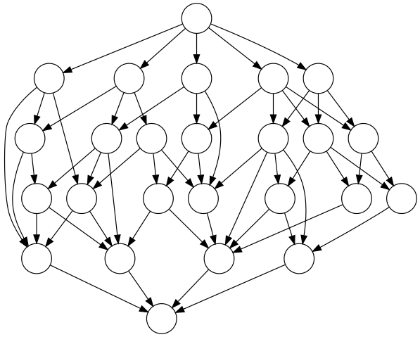
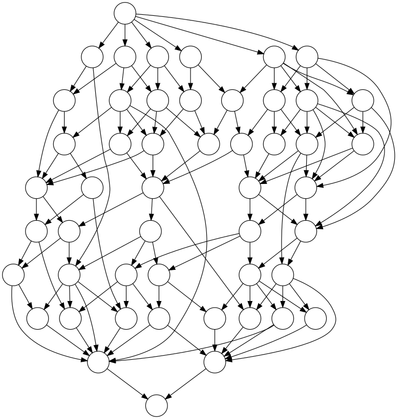
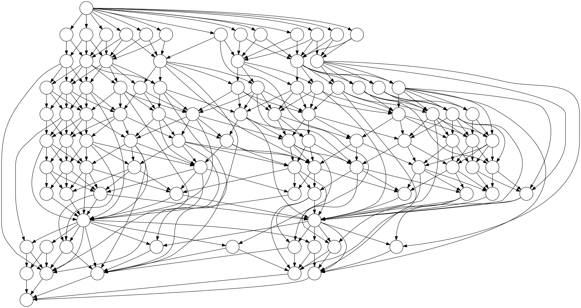
Figure 4: Three example graphs from the layered graph family with (from left) 25, 50, and 100 nodes, generated using the algorithm we describe in the text. One can clearly make out the layered structure and easily remark the presence of skip connections.

Finally, we specify the assignment of memory costs to the nodes. In the layered graph model, we have both output memory costs $\left(m_{i}\right)_{i=1}^{|V|}$ and parameter costs $\left(p_{i}\right)_{i=1}^{|V|}$, where the output cost is the memory usage of the output of an operation, and the parameter cost the one of a variable necessary to execute the operation; for example, if the operation at node $i$ were a matrix multiplication, $\boldsymbol{y}=M\boldsymbol{x}$, $o_{i}$ would be the memory usage of $\boldsymbol{y}$ and $p_{i}$ the one of the matrix $M$. The parameter cost of operation $\sigma_{t}$ during a sequence is added to the memory usage at time $t$, but not to the cost at subsequent steps since the memory associated to it can be de-allocated as soon as the operation has been executed.In particular, the memory utilization cost $M_{t}$ in (2) gets modified to the following:

$$M_{t}=I_{t-1}+m(\sigma_{t})+p(\sigma_{t})$$ (15)

where $I_{t}$ is defined in (3). Both costs are randomly drawn from a simple mixture of Gaussians $\text{GMM}(\mathbf{w},\mathbf{\mu},\mathbf{\sigma})\equiv\sum_{i=1}^{4}w_{i}\mathcal{N}(\mu_{i},\sigma_{i})$ projected on to the positive reals,

$$m_{i}\sim\text{GMM}(\mathbf{w},\mathbf{\mu},\mathbf{\sigma})\big{|}_{\mathbb{R}_{+}},~{}~{}~{}~{}p_{i}\sim\text{GMM}(\mathbf{w},\mathbf{\mu},\mathbf{\sigma}))\big{|}_{\mathbb{R}_{+}}.$$ (16)

To align the costs assignment with the real world computation graphs, instead of sampling the memory costs for each node $n$, we sample one output cost $m_{l}$ and parameter cost $p_{l}$ for each layer $l$ and assign the costs $m_{l},p_{l}$ to each node in layer $l$. This is because many real world computation graphs are a tiled version of the original precedence graph of compute nodes where each node is broken down into a layer of nodes with similar shape and parameter requirements. This concludes the description of our dataset generation algorithm. For the sake of reproducibility, we report below the value we took for all the user-defined parameters mentioned in this section:

• Variability of number of nodes per layer $\sigma_{\mathcal{N}}=0.75$

• Edge density $\rho_{E}=0.2$

• Skip connection density $\rho_{S}=0.14$

• Means of the Gaussian mixture $(\mu_{1},\mu_{2},\mu_{3},\mu_{4})=(0.5,1,3,5)$

• Standard deviations of the Gaussian mixture $(\sigma_{1},\sigma_{2},\sigma_{3},\sigma_{4})=(0.5,1,1,1)$

• Weights of the Gaussian mixture $(w_{1},w_{2},w_{3},w_{4})=(0.3,0.3,0.3,0.1)$

Appendix B Decoder Ablation study

In order to measure the effectiveness of our architecture we perform ablation experiments to study the effect of changing the decoder to an auto-regressive decoder and changing both the encoder and the decoder (Table 4).

We compare the performance of our architecture with the model which uses topoformer as an encoder but uses an auto-regressive decoder. We adapt the decoder designed for the TSP problem [6] for our memory-minimization problem. The decoder of [6] uses a notion of context node for decoding and at each decoding step using a series of multi-head attention with the context node arrives at the distribution of the next node to be selected for the order. We modify the masking procedure in the decoder of [6] to mask out all the nodes which are not present in the set of feasible next nodes $\mathcal{S}(\sigma_{1:t-1},G)$.

We also conduct an experiment by changing both the encoder and decoder by adapting the model of [6] to our problem. We adapt the auto-regressive decoder of [6] as described above. [6] uses a fully connected transformer as an encoder since the underlying graph in TSP is a fully connected graph. We modify the encoder of [6] to do message passing only on the edges of our input DAG so that it can exploit the topological structure of the graph in the encoding stage. We refer to this model as "GNN encoder + AR decoder" in table 4.

Table 4: Comparison with Auto-regressive decoding

Algorithm	500-node graphs		1000-node graphs
	% gap from	run time	% gap from	run time
	approx. DP	[$s$]	approx. DP	[$s$]
GNN encoder + AR decoder
✓Greedy	6.13 $\pm$ 0.58	1.66 $\pm$ 0.01	1.84 $\pm$ 0.39	3.34 $\pm$ 0.02
✓Sample	4.71 $\pm$ 0.56	1.76 $\pm$ 0.01	1.38 $\pm$ 0.37	3.59 $\pm$ 0.02
✓Beam search	4.87 $\pm$ 0.61	4.01 $\pm$ 0.02	2.09 $\pm$ 0.41	7.90 $\pm$ 0.05
Topoformer + AR decoder
✓Greedy	4.43 $\pm$ 0.55	1.53 $\pm$ 0.01	0.53 $\pm$ 0.35	3.05 $\pm$ 0.02
✓Sample	3.33 $\pm$ 0.51	1.7 $\pm$ 0.01	0.05 $\pm$ 0.35	3.38 $\pm$ 0.02
✓Beam search	3.14 $\pm$ 0.52	4.27 $\pm$ 0.04	0.13 $\pm$ 0.36	7.90 $\pm$ 0.05
Topoformer + NAR decoder (Ours)
✓Greedy	4.31 $\pm$ 0.56	1.04 $\pm$ 0.01	0.47 $\pm$ 0.36	1.53 $\pm$ 0.01
✓Sample	3.35 $\pm$ 0.52	1.21 $\pm$ 0.01	0.09 $\pm$ 0.35	1.78 $\pm$ 0.01
✓Beam search	3.08 $\pm$ 0.51	4.15 $\pm$ 0.02	0.2 $\pm$ 0.36	5.57 $\pm$ 0.05

We train both the models: "GNN encoder + AR decoder" and "Topoformer + AR decoder" on the layered graph dataset of 500 node graphs. We evaluate the performance of the trained model on the test set (300 graphs) of 500 node and 1000 node graphs. We use a sample size and beam width of 16 for 500 node graphs and a sample size and beam width of 8 for 1000 node graphs. We use a smaller sample size for 1000 node graphs due to GPU memory issues with the auto-regressive decoder approaches.

Table 4 shows the mean and the 95% confidence interval of the % gap from approximate DP and run time for the three approaches on 500 and 1000 node graphs. We note that the performance of topoformer with AR decoder is quite close to our model for both 500 and 1000 node graphs. However, our model can run inference 2x faster than topoformer with AR decoder on 1000 graphs nodes (in greedy mode). Also, our model outperforms the adaptation of [6] attention based GNN encoder and AR decoder to our problem both in terms of memory cost of sequence and run time. This shows the merit of our topoformer architecture over using a traditional GNN architecture which does message passing only on the input graph.

Appendix C Training and Model details

C.1 Training

We train our model using the ADAM optimizer with the initial learning rate of $10^{-4}$ and learning rate decay factor of $0.996$ per epoch. We use a batch size of $8$ for training our model. The training and testing of our model is done on a single GPU (Nvidia Tesla V-100) with $32$ GB memory. We trained our model for 326 epochs on the synthetic graph dataset where in each epoch we provide 1000 training graphs. Also, we provide a new training set in each epoch so that we do not overfit our model on a fixed training set. We found the training to be fairly stable, and it converged in about 1-2 days.

C.2 Model architecture

We use topoformer with number of layers $n_{layers}=4$, embedding dimension $d=256$, number of heads $n_{heads}=10$ for each MHA operation on the seven graphs listed in section 4.1 and the query and value dimension of $64$ for each head of MHA. The MLP used in (5) consists of a linear layer ($d_{input}=d_{output}=256$) with GELU activation followed by another linear layer ($d_{input}=d_{output}=256$). The MLP used in (7) to generate the node priorities consists of a linear layer ($d_{input}=d_{output}=256$) with RELU activation followed by another linear layer ($d_{input}=256,d_{output}=1$). In order to restrict the range of priority values, we also normalize the priorities of the nodes used for the decoding as follows:

$$\tilde{y}_{i}=\alpha\times\frac{y_{i}-\text{mean}(\mathbf{y})}{\text{std}(\mathbf{y})}$$ (17)

where $\mathbf{y}=\left[y_{1},y_{2},\ldots,y_{|V|}\right]$ and $\alpha$ is a hyperparamter. We set $\alpha=5$ for our experiments.

C.3 Baselines

We provide more details about the dynamic programming baselines used in our experiments to compare the performance of our model

• Depth-First Dynamic Programming (DP). Topological orders are generated in a depth-first manner (with backtracking) where next node is picked randomly among available candidates. Branch exploration is terminated if 1) the same set of nodes are in the partial sequence as a branch that has been already explored - only the lowest cost partial sequence is retained (dynamic programming approach), and 2) if the current partial cost is already higher than the lowest cost of any full sequence already found (cost increases monotonically). This algorithm will eventually find the global optimal order, though the run time for doing so is expected to be at least exponential in |V| [2]; it is however able to return at least one complete sequence in time $O(|V|+|E|)$ [34] in the worst case, same as DFS. In our implementation, we set a wall time of one hour and pick the best complete path found. We observe that for our synthetic layered graphs, if the graph size is as small as $|V|=100$, we can actually find the optimal sequence in most cases within the one hour budget. We ran this algorithm on a CPU machine with Intel(R) Xeon(R) W-2123 CPU @ 3.60GHz

• Approximate DP. We define the state space $S$ as the space including a set of all nodes for each partial sequence (which ignores the ordering information) and the action space for each state as the space of all possible next-node choices at that state (based on the topological structure). As an example for the state representation, if there is a partial sequence $5\rightarrow 2\rightarrow 4\rightarrow 3\rightarrow 1$, the corresponding state is $\{1,2,3,4,5\}$. With the empty set $\emptyset$ being an initial state (meaning that no node has been added), we consider a state transition model that adds an action (a node) to a state and creates a successor state. Specifically, we can partition $S$ into $S_{0}\cup S_{1}\cup\cdots\cup S_{|V|}$, where $S_{t}$ is the space including a set of all nodes for each length-$t$ partial sequence (note that $S_{0}=\{\emptyset\}$). At every iteration $t=0,1,...,|V|-1$, the algorithm takes $S_{t}$ and assumes that we have (1) the minimum cost and (2) the best partial sequence for each state in $S_{t}$, where the minimum cost is over all feasible partial sequences corresponding to the state. Then, for each successor state in $S_{t+1}$, the algorithm computes the minimum cost and the best partial sequence for reaching out that state.

  It should be noted that the algorithm gives an exact solution if the amount of time and memory resource is sufficient, e.g., an exact solution can be found for 100-node graphs. However, due to the practical resource limitation, we only keep top-$K$ elements of $S_{t+1}$ for each iteration $t$ based on costs. We use the beam size $K=100,000$ for all experiments, and Nvidia Tesla V-100 is used for parallel computation across multiple states for each iteration.

C.4 Baseline policy

The baseline $b(G)$ used in the policy gradient update is generated using the greedy rollout of the baseline policy. The baseline policy is also an instance of our model which is updated regularly during the course of training. At the end of each epoch, if the performance of the model being trained becomes better than the baseline model (in greedy inference mode) on a set of validation graphs then we copy the weights of the trained mode to the baseline model.

C.5 Input features and initial node embedding

We use the following as the input features $x_{j}$ for node $j$:

1. Output memory cost $m_{j}$ and parameter memory cost $p_{j}$

2. In-degree and out-degree of the node

3. Minimum and maximum distance (in terms of hop count) of the node from the source and target node

We normalize each entry of the input node feature across the nodes so that the features lie between $0$ and $1$ making it invariant with respect to the graph size. To be precise, the $i^{th}$ entry of the normalized input feature of node $j$ is given as $\bar{x}^{i}_{j}=\frac{x^{i}_{j}}{\max_{n}x^{i}_{n}}$. We also augment the node features with the Laplacian positional encodings (PE) [35] of dimension 20. We compute the laplacian PE using the laplacian matrix of the undirected DAG where all the directed edges are converted to undirected edges. Finally, the initial embedding $h^{0}_{j}$ for node $j$ is obtained by passing $\bar{x}_{j}$ through a linear layer.

References

- [1] P. Toth and D. Vigo, Vehicle routing: problems, methods, and applications. SIAM, 2014.
- [2] B. H. Ahn, J. Lee, J. M. Lin, H.-P. Cheng, J. Hou, and H. Esmaeilzadeh, “Ordering chaos: Memory-aware scheduling of irregularly wired neural networks for edge devices,” Proceedings of Machine Learning and Systems, vol. 2, pp. 44–57, 2020.
- [3] C. H. Papadimitriou and K. Steiglitz, Combinatorial optimization: algorithms and complexity. Courier Corporation, 1998.
- [4] G. Brightwell and P. Winkler, “Counting linear extensions is p-complete,” in Proceedings Annual ACM Symposium on Theory of Computing, 1991, p. 175–181. [Online]. Available: https://doi.org/10.1145/103418.103441
- [5] Y. Bengio, A. Lodi, and A. Prouvost, “Machine learning for combinatorial optimization: a methodological tour d’horizon,” European Journal of Operational Research, vol. 290, no. 2, pp. 405–421, 2021.
- [6] W. Kool, H. van Hoof, and M. Welling, “Attention, learn to solve routing problems!” in International Conference on Learning Representations, 2019. [Online]. Available: https://openreview.net/forum?id=ByxBFsRqYm
- [7] L. Xin, W. Song, Z. Cao, and J. Zhang, “NeuroLKH: Combining deep learning model with lin-kernighan-helsgaun heuristic for solving the traveling salesman problem,” in Advances in Neural Information Processing Systems, 2021. [Online]. Available: https://openreview.net/forum?id=VKVShLsAuZ
- [8] C. K. Joshi, Q. Cappart, L.-M. Rousseau, and T. Laurent, “Learning TSP requires rethinking generalization,” in International Conference on Principles and Practice of Constraint Programming, 2021.
- [9] A. Correia, D. E. Worrall, and R. Bondesan, “Neural simulated annealing,” 2022. [Online]. Available: https://openreview.net/forum?id=bHqI0DvSIId
- [10] W. J. Cook, In pursuit of the traveling salesman. Princeton University Press, 2011.
- [11] A. Paliwal, F. Gimeno, V. Nair, Y. Li, M. Lubin, P. Kohli, and O. Vinyals, “Reinforced genetic algorithm learning for optimizing computation graphs,” in International Conference on Learning Representations, 2020. [Online]. Available: https://openreview.net/forum?id=rkxDoJBYPB
- [12] Y. Zhou, S. Roy, A. Abdolrashidi, D. Wong, P. Ma, Q. Xu, H. Liu, P. Phothilimtha, S. Wang, A. Goldie et al., “Transferable graph optimizers for ML compilers,” Advances in Neural Information Processing Systems, vol. 33, pp. 13 844–13 855, 2020.
- [13] R. S. Sutton and A. G. Barto, Reinforcement learning: An introduction. MIT press, 2018.
- [14] E. Khalil, H. Dai, Y. Zhang, B. Dilkina, and L. Song, “Learning combinatorial optimization algorithms over graphs,” Advances in neural information processing systems, vol. 30, 2017.
- [15] I. Bello*, H. Pham*, Q. V. Le, M. Norouzi, and S. Bengio, “Neural combinatorial optimization with reinforcement learning,” 2017. [Online]. Available: https://openreview.net/forum?id=rJY3vK9eg
- [16] G. Mena, D. Belanger, S. Linderman, and J. Snoek, “Learning latent permutations with gumbel-sinkhorn networks,” in International Conference on Learning Representations, 2018.
- [17] S. Linderman, G. Mena, H. Cooper, L. Paninski, and J. Cunningham, “Reparameterizing the Birkhoff polytope for variational permutation inference,” in Proceedings of the International Conference on Artificial Intelligence and Statistics, vol. 84, 09–11 Apr 2018, pp. 1618–1627. [Online]. Available: https://proceedings.mlr.press/v84/linderman18a.html
- [18] A. Gadetsky, K. Struminsky, C. Robinson, N. Quadrianto, and D. Vetrov, “Low-variance black-box gradient estimates for the plackett-luce distribution,” in Proceedings of the AAAI Conference on Artificial Intelligence, vol. 34, no. 06, 2020, pp. 10 126–10 135.
- [19] B. Steiner, C. Cummins, H. He, and H. Leather, “Value learning for throughput optimization of deep learning workloads,” Proceedings of Machine Learning and Systems, vol. 3, pp. 323–334, 2021.
- [20] Z. Wu, S. Pan, F. Chen, G. Long, C. Zhang, and S. Y. Philip, “A comprehensive survey on graph neural networks,” IEEE transactions on neural networks and learning systems, vol. 32, no. 1, pp. 4–24, 2020.
- [21] P. W. Battaglia, J. B. Hamrick, V. Bapst, A. Sanchez-Gonzalez, V. Zambaldi, M. Malinowski, A. Tacchetti, D. Raposo, A. Santoro, R. Faulkner et al., “Relational inductive biases, deep learning, and graph networks,” arXiv preprint arXiv:1806.01261, 2018.
- [22] V. Thost and J. Chen, “Directed acyclic graph neural networks,” in International Conference on Learning Representations, 2020.
- [23] M. Zhang, S. Jiang, Z. Cui, R. Garnett, and Y. Chen, “D-VAE: A variational autoencoder for directed acyclic graphs,” Advances in Neural Information Processing Systems, vol. 32, 2019.
- [24] M. Bianchini, M. Gori, and F. Scarselli, “Recursive processing of directed acyclic graphs,” in Neural Nets WIRN Vietri-01, 2002, pp. 96–101.
- [25] C. Ying, T. Cai, S. Luo, S. Zheng, G. Ke, D. He, Y. Shen, and T.-Y. Liu, “Do transformers really perform badly for graph representation?” Advances in Neural Information Processing Systems, vol. 34, 2021.
- [26] R. Sato, “A survey on the expressive power of graph neural networks,” 2020. [Online]. Available: https://arxiv.org/abs/2003.04078
- [27] T. N. Kipf and M. Welling, “Semi-supervised classification with graph convolutional networks,” in International Conference on Learning Representations, 2017.
- [28] P. Veličković, G. Cucurull, A. Casanova, A. Romero, P. Liò, and Y. Bengio, “Graph attention networks,” in International Conference on Learning Representations, 2018. [Online]. Available: https://openreview.net/forum?id=rJXMpikCZ
- [29] R. Wang, Z. Hua, G. Liu, J. Zhang, J. Yan, F. Qi, S. Yang, J. ZHOU, and X. Yang, “A bi-level framework for learning to solve combinatorial optimization on graphs,” in Advances in Neural Information Processing Systems, 2021.
- [30] A. Vaswani, N. Shazeer, N. Parmar, J. Uszkoreit, L. Jones, A. N. Gomez, Ł. Kaiser, and I. Polosukhin, “Attention is all you need,” Advances in neural information processing systems, vol. 30, 2017.
- [31] R. Xiong, Y. Yang, D. He, K. Zheng, S. Zheng, C. Xing, H. Zhang, Y. Lan, L. Wang, and T. Liu, “On layer normalization in the transformer architecture,” in International Conference on Machine Learning. PMLR, 2020, pp. 10 524–10 533.
- [32] J. L. Ba, J. R. Kiros, and G. E. Hinton, “Layer normalization,” in NIPS Deep Learning Symposium, 2016. [Online]. Available: https://arxiv.org/pdf/1607.06450v1.pdf
- [33] R. J. Williams, “Simple statistical gradient-following algorithms for connectionist reinforcement learning,” Machine learning, vol. 8, no. 3, pp. 229–256, 1992.
- [34] A. B. Kahn, “Topological sorting of large networks,” Communications of the ACM, vol. 5, no. 11, pp. 558–562, 1962.
- [35] V. P. Dwivedi and X. Bresson, “A generalization of transformer networks to graphs,” arXiv preprint arXiv:2012.09699, 2020.