Fast Radix-32 Approximate DFTs for 1024-Beam Digital RF Beamforming

The discrete Fourier transform (DFT) is widely employed for multi-beam digital beamforming. The DFT can be efficiently implemented through the use of fast Fourier transform (FFT) algorithms, thus reducing chip area, power consumption, processing time, and consumption of other hardware resources. This paper proposes three new hybrid DFT 1024-point DFT approximations and their respective fast algorithms. These approximate DFT (ADFT) algorithms have significantly reduced circuit complexity and power consumption compared to traditional FFT approaches while trading off a subtle loss in computational precision which is acceptable for digital beamforming applications in RF antenna implementations. ADFT algorithms have not been introduced for beamforming beyond $N=32$, but this paper anticipates the need for massively large adaptive arrays for future 5G and 6G systems. Digital CMOS circuit designs for the ADFTs show the resulting improvements in both circuit complexity and power consumption metrics. Simulation results show similar or lower critical path delay with up to 48.5% lower chip area compared to a standard Cooley-Tukey FFT. The time-area and dynamic power metrics are reduced up to 66.0%. The 1024-point ADFT beamformers produce signal-to-noise ratio (SNR) gains between 29.2–30.1 dB, which is a loss of $\leq$ 0.9 dB SNR gain compared to exact 1024-point DFT beamformers (worst case) realizable at using an FFT.

Keywords
Fourier Transform, Discrete Fourier Transform, Approximation, VLSI, DFT, FFT, Radix, Fast Algorithm, Beamforming, Beamsteering, 5G, MIMO, Massive MIMO.

The discrete Fourier transform (DFT) is a linear transform that is widely applied to convert a sampled signal into a representation over the discrete frequency domain. Fully-digital transmit and receive aperture arrays for radio-frequency (RF) spectrum sensing, communications, and radar use the DFT for multi-beam beamforming. For example, simultaneous receiver beams are imperative for high-capacity multi-input multi-output (MIMO) wireless communication systems. Joint spatial division and multiplexing (JSDM) is an approach to multi-user MIMO downlinks that exploits the structure of channel correlations in order to allow a large number of antennas at the base station while requiring reduced-dimensional channel state information at the transmitter [50, 41]. This uses a multi-user MIMO downlink precoder obtained from an array pre-beamforming matrix, and incurs no loss of optimality for a large number of array elements. A DFT-based pre-beamforming matrix is near-optimal for uniform linear arrays (ULAs) of antennas, and requires only coarse information about the users’ angles of arrival and angular spread [2].

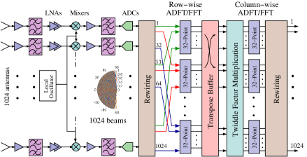
Figure 1: Beamforming architecture of a 1024-element ULA receiver using the proposed method. The rewiring block performs spatial multiplexing over the incoming in the input and the transformed signal at the output (see Fig. 5).

The $N$-point DFT computes $N$ uniformly spaced frequency domain outputs (“bins”) using $N$ uniformly sampled discrete signal values by means of an $N\times N$ transform matrix [12]. Because implementations of the multiplication operation requires more chip area (or processing time, for non-parallelized software implementations) compared to addition operations, the computational complexity of computing the DFT is expressed in terms of the multiplication count [10]. The required number of multiplications depends on the fast algorithm employed for the particular transform length $N$ in consideration. The computational complexity of the $N$-point DFT using direct matrix-vector multiplication is $\mathcal{O}(N^{2})$ where $\mathcal{O}(\cdot)$ represents the “big O” notation for asymptotic complexity [32, 27, 4].

The computational complexity of computing the $N$-point DFT can be reduced via fast Fourier transforms (FFTs), which are fast algorithms for realizing DFTs that reduce the computational complexity to $\mathcal{O}(N\log_{2}N)$ [10]. Thus, multiple DFT beams for both wireless communications applications (e.g., JSDM) and multi-beam radar/imaging systems are often generated by applying an $N$-point spatial FFT to each temporal sample acquired by the ULA [18, 13].

The search for particular $N$-point FFT methods that minimize the multiplicative complexity is a separate field of research in signal processing, computer science, and applied mathematics, with a multitude of algorithms and implementations available [10, 49, 25, 7, 22]. In [19], the theoretical lower bound for the DFT multiplicative complexity was established as a function of $N$. All FFT algorithms use sparse factorizations of the DFT matrix to provide accurate implementations of the DFT at an arithmetic complexity that approaches this lower bound. However, such high accuracy is of limited practical relevance in digital multi-beam RF beamforming applications, such as radar signal processing, where the accuracy of the results is limited by other system parameters or environmental conditions (e.g., thermal noise in a receiver, or the practical implementation of an antenna radiation pattern compared to ideal, harmonic distortion in a microwave mixer or amplifier). In such applications, relentless pursuit of high accuracy in the exact computation of the DFT is not relevant in terms of overall performance, and smart system designers can exploit this fact for power and cost optimization. High-precision VLSI implementation of FFT algorithms may result in unnecessarily large circuits, exaggerated critical path delays, and wasted power. All of those factors contribute to higher-cost circuits, reduced frequency of operation, and higher operation costs. This is because digital multipliers demand a large amount of circuit resources when compared to simple adders. This makes the reduction of the number of multipliers in a given system crucial when chip area and power must be conserved and high-speed operation is desirable. In particular, the adoption of approximate DFT (ADFT) computations opens up new possibilities for fast algorithms which do not compute the DFT in the strictest mathematical sense, but nevertheless can be good enough for digital multi-beam RF beamforming applications, particularly at mmwave frequencies and above, where reproducibility of antenna patterns become more problematic. Because ADFT applications are able to realize much greater efficiencies than the theoretical lower bound $N$ for an $N$-point DFT proposed in [19], ADFT computations allow greater reductions in computational complexity than traditional FFTs, albeit at the cost of a deterministic loss in performance, namely a small increase in worst-case side-lobe level [6].

The ever increasing data rate demands of wireless communications led to the exploration of millimeter-wave (mmW)/sub-THz/THz frequencies in 5G cellular networks [34, 35], where larger antenna array sizes (e.g. $N=64,\leavevmode\nobreak\ 128,\leavevmode\nobreak\ 256$) for beamforming and massive MIMO have become a general requirement [9]. For example, IoT and robotics applications in emerging fifth-generation (5G) and beyond mobile wireless networks will require 6D positioning, which involves both spatial position and device orientation (role, pitch, yaw) which require new algorithms that can benefit from large number of closely packed low-complexity digital beams [46, 28, 41]. A similar need occurs in the design of systems for intelligent surfaces which provide means of communication without line-of-sight [42]. In fact mmW-based 5G MIMO cellular systems are already being deployed [1]. Moreover, ongoing research in the sub-THz range [20, 51, 26, 38, 11, 36, 23, 31, 8, 41] suggests that the W and G bands will be commercially available within the next 5-10 years. Such sub-THz carrier frequencies require large amounts of beamforming gain to mitigate free-space path loss in the first meter of propagation from the antenna [35, 41, 48, 47]. Thus, communication systems at these frequencies would require much larger numbers of antenna elements in the transceiver arrays; array sizes of the order of $N=1000$ elements would not be unrealistic for future sixth generation (6G) cellular systems. Nevertheless, to the best of our knowledge, DFT approximations in the literature are limited to $N\leq 32$.

In this paper, we address this important beamforming challenge by introducing three new approximations to the very large N = 1024 (1024-point) DFT. Fast algorithms that allow low-complexity implementations of these approximations are also developed and shown to provide remarkable accuracy with significant cost and power reduction compared to DFT and FFT approaches. The proposed 1024-point ADFTs are based on a recently proposed 32-point DFT approximation and multiplierless fast algorithm [40, 27] that furnish a “reasonable” approximation of the 32-point DFT albeit without using multiplications (i.e., using an adder-only signal flow graph). The 1024-point exact DFT can be expressed in terms of 32-point DFT. We use this fact to derive an approximation for the 1024-point DFT matrix by means for our earlier 32-point ADFT. In particular, we propose three different 1024-point transforms with different trade-offs in computational complexity and computational accuracy compared to the baseline exact DFT. These three transforms differ from each other based on the use of 32-point ADFT in the derivation and they can be used to replace the FFT while generating $N=1024$ beams from a 1024-element ULA as shown in Fig. 1.

The paper is organized as follows. Section 1 reviews the DFT and selected popular FFT algorithms. In Section 2, we discuss the mathematical background for the 32-point DFT approximation introduced in [40] and describe its associated fast algorithm in matrix form. In Section 3, we present 1024-point DFT approximations and discuss three different algorithms to implement them. Section 4 explores the digital VLSI realization of the proposed 1024-point DFT approximations. In Section 5, we summarize our conclusions.

1 Review of the DFT and FFT

In order to understand the method used to create accurate ADFT algorithms, we will discuss the mathematical background related to the DFT definition and FFT algorithms.

1.1 Mathematical Definition of the DFT

Let the vector $\mathbf{x}=\begin{bmatrix}x[0]&x[1]&\ldots&x[N-1]\end{bmatrix}^{\top}$ represent a signal with $N$ samples. The DFT maps the input signal $\mathbf{x}$ into an output signal $\mathbf{X}=\begin{bmatrix}X[0]&X[1]&\cdots&X[N-1]\end{bmatrix}^{\top}$ according to the following relationship:

$$X[k] \triangleq\frac{1}{\sqrt{N}}\sum_{n=0}^{N-1}x[n]\cdot\omega_{N}^{nk},\quad k=0,1,\ldots,N-1,$$ (1)

where $\omega_{N}=e^{-j\frac{2\pi}{N}}$ is the $N$th root of unity and $j\triangleq\sqrt{-1}$. On the other hand, the inverse DFT (IDFT) is given as

$$x[n] =\frac{1}{\sqrt{N}}\sum_{k=0}^{N-1}X[k]\cdot\omega_{N}^{-nk},\quad n=0,1,\ldots,N-1.$$ (2)

The DFT of $\mathbf{x}$ can be expressed through a matrix-vector multiplication $\mathbf{X}=\mathbf{F}_{N}\cdot\mathbf{x}$, where

$$\mathbf{F}_{N}=\frac{1}{\sqrt{N}}\left[\begin{smallmatrix}1&1&1&\ldots&1\\ 1&\omega_{N}&\omega_{N}^{2}&\ldots&\omega_{N}^{(N-1)}\\ 1&\omega_{N}^{2}&\omega_{N}^{4}&\ldots&\omega_{N}^{2(N-1)}\\ 1&\omega_{N}^{3}&\omega_{N}^{6}&\ldots&\omega_{N}^{3(N-1)}\\ \vdots&\vdots&\vdots&\ddots&\vdots\\ 1&\omega_{N}^{(N-1)}&\omega_{N}^{2(N-1)}&\ldots&\omega_{N}^{(N-1)(N-1)}\\ \end{smallmatrix}\right]$$ (3)

is the $N$-point DFT matrix [33].

1.2 FFT Algorithms

DFT was originally the cornerstone of primitive DSP, until the FFT was found to be vastly more efficient. Here we extend FFTs to become ADFTs. The computational complexity associated with performing the $N$-point DFT operation in direct form is $\mathcal{O}(N^{2})$. This complexity is prohibitive for most engineering applications since a high number of operations accounts for (i) higher energy consumption; (ii) higher latency; (iii) higher number of gates; and, in consequence, (iv) higher chance of system failure. To address these issues, FFT factorizations furnish a product of sparse (mostly zeros) matrices that reduces the DFT computational complexity to $\mathcal{O}(N\log N)$. Different FFT algorithms can be identified in the literature [14, 16, 43, 44]. Here we consider three popular algorithms, namely i) the Cooley-Tukey FFT [10], ii) the split-radix FFT [16], and iii) the Winograd FFT [45]; each of these is briefly described below.

1.2.1 Cooley-Tukey Algorithm

A very popular form of the classical Cooley-Tukey algorithm is the radix-2 decimation-in-time FFT, which splits the $N$-point DFT computation into two $N/2$-point DFT computations resulting in an overall reduced complexity [14]. Recursive use of this algorithm reduces the number of multiplications of the DFT from $\mathcal{O}(N^{2})$ down to $\mathcal{O}(N\log_{2}N)$.

1.2.2 Split-radix Algorithm

This is a variant of the Cooley-Tukey FFT algorithm which uses a blend of radix-2 and radix-4 by recursively expressing the $N$-point DFT in terms of one $N/2$-point DFT and two $N/4$-point DFT instantiations [16]. The split-radix algorithm can reduce the overall number of additions required to compute DFTs of sizes that are powers of two without increasing the number of multiplications [21].

1.2.3 Winograd Algorithm

The Winograd algorithm implements an efficient FFT and exploits the multiplicative structure on the data indexing of DFT and converts it into a cyclic convolution computation [43, 44]. In several particular cases, the Winograd algorithm achieves the theoretical minimum multiplicative complexity [19] as shown in [43] making it more efficient over the Cooley-Tukey and radix. For large DFT block lengths that can be decomposed as a product of small primes, the Winograd algorithm achieves nearly-linear complexity [10].

1.3 Matrix Representation of the $N^{2}$-point DFT in terms of the $N$-point DFT

Now we will use the matrix definition in sub section 1.1 to derive a matrix representation for the computation of the $N^{2}$-point DFT in terms of the $N$-point DFT via a radix-$N$ FFT approach. The goal of this is to derive a 1024-point DFT in terms of 32-point DFT. Generally speaking, the $N^{2}$-point DFT computation corresponds to a vector-matrix multiplication with a $N^{2}\times N^{2}$ matrix transformation:

$$\mathbf{X}=\mathbf{F}_{N^{2}}\cdot\mathbf{x}.$$ (4)

The expression in (4) can be rewritten by directly invoking the Cooley-Tukey algorithm in its more general form as detailed in [10, p. 69]. By explicitly following the Cooley-Tukey algorithm, the $N^{2}$-point DFT can be computed by means of:

1. address-shuffling the input column vector into a 2D $N\times N$ array;

2. computing the $N$-point DFT of each array column using FFTs;

3. element-wise multiplying the twiddle-factors (twiddle factors are the coefficients containing roots of unity in the DFT matrix [10]);

4. computing the $N$-point DFT of each resulting row using FFTs; and

5. undoing the address shuffling to convert the obtained 2D array into the final output column vector.

The 1D to 2D mapping can be accomplished by means of the inverse vectorization operator $\operatorname{invvec}(\cdot)$ [17] (Cf. [30, 29]) which obeys the following mapping:

$$\operatorname{invvec}\left(\begin{bmatrix}x_{0}\\ x_{1}\\ \vdots\\ x_{N^{2}}\end{bmatrix}\right)=\begin{bmatrix}x_{0}&x_{N}&\cdots&x_{N(N-1)}\\ x_{1}&x_{N+1}&\cdots&x_{N(N-1)+1}\\ \vdots&\vdots&\ddots&\vdots\\ x_{N-1}&x_{2N-1}&\cdots&x_{N^{2}-1}\end{bmatrix}.$$ (5)

Based on the 1D to 2D mapping in Eqn. (5) we can show that the $N^{2}$-point DFT given in (4) can be represented in the following matrix expression based on the Cooley-Tukey algorithm:

$$\mathbf{X}=\operatorname{vec}\left(\left\{\mathbf{F}_{N}\cdot\left[\mathbf{\Omega}_{N}\circ\left(\mathbf{F}_{N}\cdot(\operatorname{invvec}(\mathbf{x}))^{\top}\right)\right]^{\top}\right\}^{\top}\right),$$ (6)

where $\operatorname{vec}(\cdot)$ is the matrix vectorization operator [37, p. 239], $\circ$ is the Hadamard element-wise multiplication [37, p. 251], the superscript ^⊤ denotes simple transposition (non Hermitian), and $\mathbf{\Omega}_{N}$ is the twiddle-factor matrix given by $\mathbf{\Omega}_{N}=(\omega_{N^{2}}^{m\cdot n})_{m,n=0,1,\ldots,N}$. Noting that $\mathbf{\Omega}_{N}^{\top}=\mathbf{\Omega}_{N}$, (6) can be further simplified. In particular, for $N=1024=32^{2}$, we have

$$\mathbf{X}=\operatorname{vec}\left(\left[\mathbf{\Omega}_{32}\circ\left(\mathbf{F}_{32}\cdot(\operatorname{invvec}(\mathbf{x}))^{\top}\right)\right]\cdot\mathbf{F}_{32}^{\top}\right).$$ (7)

The inner DFT call corresponds to row-wise transformation of $\operatorname{invvec}(\mathbf{x})$, whereas the outer DFT performs column-wise transformations on the resulting intermediate computation. The formulation shown in (7) is the fundamental expression on which the proposed approximations (eg. ADFTs) in this work are based.

2 Multiplierless 32-point ADFT

In this section, the adopted multiplierless 32-point ADFT, first introduced in [40, 27], is presented, and its complexity and error analysis are discussed . This is critical for understanding as the 1024-point ADFT is realized using 32-point ADFT as the main building block.

2.1 Matrix Representation

The considered 32-point ADFT matrix denoted by $\hat{\mathbf{F}}_{32}$ can be computed through a product of sparse matrices whose real and imaginary parts of its coefficients contains only $\pm 1$ entries. Such simple arithmetic leads to hardware designs that can be realized with adders only.

To present the factorization of $\hat{\mathbf{F}}_{32}$, we need the auxiliary structures in eq. (8)- (19), since the auxiliary factors are key for matrix factorization. Let $\mathbf{B}_{t}$ be a $t\times t$ real matrix given by

$$\mathbf{B}_{t} =\begin{cases}\left[\hbox{}\,\vbox{\Let@\restore@math@cr\default@tag\halign{\hfil$\m@th\scriptstyle#$&&\thickspace\hfil$\m@th\scriptstyle#$\cr\mathbf{I}_{(t-1)/2}&&\bar{\mathbf{I}}_{(t-1)/2}\\ &1&\\ \bar{\mathbf{I}}_{(t-1)/2}&&-\mathbf{I}_{(t-1)/2}\crcr}}\,\right],&\text{if\leavevmode\nobreak\ $t$ is odd,}\\ \\ \left[\hbox{}\,\vbox{\Let@\restore@math@cr\default@tag\halign{\hfil$\m@th\scriptstyle#$&&\thickspace\hfil$\m@th\scriptstyle#$\cr\mathbf{I}_{t/2}&\bar{\mathbf{I}}_{t/2}\\ \bar{\mathbf{I}}_{t/2}&-\mathbf{I}_{t/2}\crcr}}\,\right],&\text{if\leavevmode\nobreak\ $t$ is even,}\end{cases}$$ (8)

where $\mathbf{I}_{k}$ and $\bar{\mathbf{I}}_{k}$ being the identity and counter-identity matrix of order ${k}$, respectively. Let also $\mathbf{Z}_{1}$, $\mathbf{Z}_{2}$, and $\mathbf{Z}_{3}$ be the following matrices (for clarity, only the non-zero elements are shown):

$$\mathbf{Z}_{1}=\left[\setcounter{MaxMatrixCols}{16}\begin{smallmatrix}1&&&&&&&&&&&&1&&&\\ &1&&&&&&&&&&&&&&\\ &&1&&&&&&&&&&&&&\\ &&&1&&&&&&&&&&&&\\ &&&&1&&&&1&&&&&&&\\ &&&&&1&&&&&&&&&&\\ &&&&&&1&&&&&&&&&\\ &&&&&&&1&&&&&&&&\\ &&&&1&&&&-1&&&&&&&\\ &&&&&&&&&1&&&&&&\\ &&&&&&&&&&1&&&&&\\ &&&&&&&&&&&1&&&&\\ 1&&&&&&&&&&&&-1&&&\\ &&&&&&&&&&&&&1&&\\ &&&&&&&&&&&&&&1&\\ &&&&&&&&&&&&&&&1\\ \end{smallmatrix}\right],$$ (9)

$$\mathbf{Z}_{2} =\left[\setcounter{MaxMatrixCols}{17}\begin{smallmatrix}1&&&&&&&&&&&&&&&&\\ &-1&&&&&&&&&&&&&&1&\\ &&1&&&&&&&&&&&&&&\\ &&&1&&&&&&1&&&&&&&\\ &&&&1&&1&&1&&&&&&&&\\ &&&&&1&&1&&&&&&&&&\\ &&&&1&&-1&&&&&&&&&&\\ &&&&&1&&-1&&&&&&&&&\\ &&&&1&&&&-1&&&&&&&&\\ &&&1&&&&&&-1&&&&&&&\\ &&&&&&&&&&1&&&&&&\\ &&&&&&&&&&&1&&1&&&\\ &&&&&&&&&&&&1&&1&&1\\ &&&&&&&&&&&1&&-1&&&\\ &&&&&&&&&&&&1&&-1&&\\ &1&&&&&&&&&&&&&&1&\\ &&&&&&&&&&&&1&&&&-1\\ \end{smallmatrix}\right],$$ (10)

and

$$\mathbf{Z}_{3} =\left[\setcounter{MaxMatrixCols}{15}\begin{smallmatrix}1&&&&1&&-1&&&&&&&&\\ &1&&&&&&&&&&&&&\\ &&1&1&&&&&&&&&&&\\ &&1&-1&&&&&&&&&&&\\ 1&&&&-1&&&&&&&&&&\\ &&&&&1&&&&&&&&&\\ 1&&&&&&1&&&&&&&&\\ &&&&&&&1&&&&&&&\\ &&&&&&&&1&&&&1&&-1\\ &&&&&&&&&1&&&&&\\ &&&&&&&&&&1&&&1&\\ &&&&&&&&&&&1&&&\\ &&&&&&&&1&&&&-1&&\\ &&&&&&&&&&1&&&-1&\\ &&&&&&&&1&&&&&&1\\ \end{smallmatrix}\right].$$ (11)

The 32-point ADFT matrix is factorized into eight sparse matrices $\mathbf{W}_{k}$, for $k=0,1,\ldots,7$, according to

$$\hat{\mathbf{F}}_{32} =\mathbf{W}_{7}\cdot\mathbf{W}_{6}\cdot\mathbf{W}_{5}\cdot\mathbf{W}_{4}\cdot\mathbf{W}_{3}\cdot\mathbf{W}_{2}\cdot\mathbf{W}_{1}\cdot\mathbf{W}_{0},$$ (12)

where

$$\mathbf{W}_{0}=\left[\begin{smallmatrix}\mathbf{B}_{17}&\\ &\mathbf{B}_{15}\end{smallmatrix}\right],\quad\mathbf{W}_{1}=\left[\begin{array}[]{c c}\mathbf{I}_{16}&\left[\begin{smallmatrix}0&\\ &\mathbf{I}_{15}\end{smallmatrix}\right]\\ \left[\begin{smallmatrix}0&\\ &\mathbf{I}_{15}\end{smallmatrix}\right]&\left[\begin{smallmatrix}1&\\ &-\mathbf{I}_{15}\end{smallmatrix}\right]\end{array}\right],$$ (15)

$$\mathbf{W}_{2} =\left[\begin{smallmatrix}\mathbf{B}_{9}&&\\ &\mathbf{B}_{7}&\\ &&\mathbf{I}_{16}\end{smallmatrix}\right],\quad\mathbf{W}_{3}=\left[\begin{smallmatrix}\mathbf{B}_{5}&&&&&&\\ &1&&&&&\\ &&\mathbf{B}_{3}&&&&\\ &&&1&&&\\ &&&&\mathbf{B}_{3}&&\\ &&&&&\mathbf{B}_{3}&\\ &&&&&&\mathbf{Z}_{1}\end{smallmatrix}\right],$$ (16)

$$\mathbf{W}_{4} =\left[\begin{smallmatrix}\mathbf{B}_{3}&&&&&&\\ &\mathbf{B}_{2}&&&&\\ &&\mathbf{B}_{4}&&&\\ &&&\mathbf{B}_{4}&&\\ &&&&\mathbf{B}_{2}&\\ &&&&&\mathbf{Z}_{2}\end{smallmatrix}\right],\quad\mathbf{W}_{5}=\left[\begin{smallmatrix}\mathbf{B}_{2}&&\\ &\mathbf{I}_{15}&\\ &&\mathbf{Z}_{3}\end{smallmatrix}\right],$$ (17)

$$\mathbf{W}_{6}=\left[\begin{smallmatrix}\mathbf{I}_{16}&\\ &\left[\setcounter{MaxMatrixCols}{16}\begin{smallmatrix}1&&&&&&&&&&&&&1&&\\ &1&&&&&&&1&&&&&&&\\ &&-1&&&&&1&&&&&&&&\\ &&&1&&&&&&&&&&&&\\ &&&&1&&&&&&&&&&&\\ &&&&&1&1&&&&&&&&&\\ &&&&&1&-1&&&&&&&&&\\ &&1&&&&&1&&&&&&&&\\ &1&&&&&&&-1&&&&&&&\\ &&&&&&&&&1&1&&&&&\\ &&&&&&&&&1&-1&&&&&\\ &&&&&&&&&&&1&&&&\\ &&&&&&&&&&&&1&&&1\\ 1&&&&&&&&&&&&&-1&&\\ &&&&&&&&&&&&&&1&\\ &&&&&&&&&&&&1&&&-1\\ \end{smallmatrix}\right]\end{smallmatrix}\right],$$ (18)

and $\mathbf{W}_{7}$ is given in (19).

2.2 Arithmetic Complexity

In this section, we study the arithmetic complexity of the proposed ADFTs by assuming execution is fully sequential. That is, we consider all algorithms execute on a sequential processor by utilizing a central processing unit (CPU) that furnishes arithmetic operations dictated by the particular algorithm. The execution time is proportional to the number of arithmetic operations, and in general, multiplication being more computationally intensive compared to addition, takes longer to execute. Therefore, the number of multiplications is the primary metric for quantification of arithmetic complexity.

The discussed 32-point ADFT has a null complexity of multiplications and no bit-shifting operations are required. The only source of arithmetic complexity is the number of additions in the factorization in (12). Considering complex inputs, the matrices $\mathbf{W}_{0}$, $\mathbf{W}_{1}$, and $\mathbf{W}_{4}$ require 60 real additions each, while the matrices $\mathbf{W}_{2}$, $\mathbf{W}_{3}$, and $\mathbf{W}_{5}$ require 28 real additions each. Similarly, the matrix $\mathbf{W}_{6}$ requires 24 real additions, while the only complex matrix in the factorization, $\mathbf{W}_{7}$, requires 60 real additions. In total, the transform $\hat{\mathbf{F}}_{32}$ thus requires 348 real additions and no bit-shifting. By comparison, the Cooley-Tukey radix-2 algorithm requires 88 real multiplications and 408 real additions [10, 16]. In contrast, the approach to represent a 32-point DFT using (4) and (7) offers $1/8$ the number of additions with no multiplications as compared to the 88 multiplications needed by Cooley-Tukey.

2.3 Error Analysis

The rows of a linear transform matrix can be understood as a finite impulse response (FIR) filter bank [32]. Savings of computation and exploitation of sparsity gives rise to slightly inaccurate representations of the frequency response of the filter bank. Thus we can assess how close the filter bank implied by the proposed (in eq. (12)) ADFT approximations are to the rows of exact DFT matrix. The filter bank frequency responses for four of the bins of the 32-point DFT, 32-point ADFT, and the corresponding error plots are shown in Fig. 2. The four bins shown are the ones corresponding the the rows of the 32-point ADFT that performs the worst in terms of frequency response; thus they can be understood as worst-case scenarios. The figure shows that the 32-point ADFT is “close enough” to the exact DFT to be useful in many practical applications, especially for wireless communications and software-defined radio (SDR) where antenna pattern, noise and semiconductor process variations induce some errors themselves: its error level of about $-10$ dB compared to the main lobe of exact DFT’s filterbank response is within the margin of error of such systems (which include both electronics and electromagnetics).

$$\mathbf{W}_{7} =\left[\setcounter{MaxMatrixCols}{32}\begin{smallmatrix}1&&&&&&&&&&&&&&&&&&&&&&&&&&&&&&&\\ &&&&&&&&&&&&&&&&&&&-j&&&&&&&&1&&&&\\ &&&&&&1&&&&-j&&&&&&&&&&&&&&&&&&&&&\\ &&&&&&&&&&&&&&&&&&&&&&&-j&&&&&-1&&&\\ &&&1&&&&&&&&&&j&&&&&&&&&&&&&&&&&&\\ &&&&&&&&&&&&&&&&&-j&&&&&&&&1&&&&&&\\ &&&&&-1&&&&-j&&&&&&&&&&&&&&&&&&&&&&\\ &&&&&&&&&&&&&&&&-1&&&&&&-j&&&&&&&&&\\ &&1&&&&&&&&&&&&&-j&&&&&&&&&&&&&&&&\\ &&&&&&&&&&&&&&&&&&&&&-j&&&&&&&&-1&&\\ &&&&&&&&1&&&&-j&&&&&&&&&&&&&&&&&&&\\ &&&&&&&&&&&&&&&&&&&&&&&&-j&&-1&&&&&\\ &&&&-1&&&&&&&&&&j&&&&&&&&&&&&&&&&&\\ &&&&&&&&&&&&&&&&&&-j&&&&&&&&&&&&&-1\\ &&&&&&&1&&&&j&&&&&&&&&&&&&&&&&&&&\\ &&&&&&&&&&&&&&&&&&&&-j&&&&&&&&&&-1&\\ &1&&&&&&&&&&&&&&&&&&&&&&&&&&&&&&\\ &&&&&&&&&&&&&&&&&&&&j&&&&&&&&&&-1&\\ &&&&&&&1&&&&-j&&&&&&&&&&&&&&&&&&&&\\ &&&&&&&&&&&&&&&&&&j&&&&&&&&&&&&&-1\\ &&&&-1&&&&&&&&&&-j&&&&&&&&&&&&&&&&&\\ &&&&&&&&&&&&&&&&&&&&&&&&j&&-1&&&&&\\ &&&&&&&&1&&&&j&&&&&&&&&&&&&&&&&&&\\ &&&&&&&&&&&&&&&&&&&&&j&&&&&&&&-1&&\\ &&1&&&&&&&&&&&&&j&&&&&&&&&&&&&&&&\\ &&&&&&&&&&&&&&&&-1&&&&&&j&&&&&&&&&\\ &&&&&-1&&&&j&&&&&&&&&&&&&&&&&&&&&&\\ &&&&&&&&&&&&&&&&&j&&&&&&&&1&&&&&&\\ &&&1&&&&&&&&&&-j&&&&&&&&&&&&&&&&&&\\ &&&&&&&&&&&&&&&&&&&&&&&j&&&&&-1&&&\\ &&&&&&1&&&&j&&&&&&&&&&&&&&&&&&&&&\\ &&&&&&&&&&&&&&&&&&&j&&&&&&&&1&&&&\\ \end{smallmatrix}\right].$$ (19)

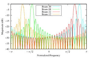
(a) 32-point DFT

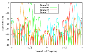
(b) 32-point ADFT

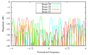
(c) Error

Figure 2: Magnitude of the filter-bank responses for (a) the exact 32-point DFT, (b) the 32-point ADFT and (c) error of the ADFT response for the least performing rows.

3 Approximations for the 1024-point DFT

3.1 Approximation Methodology

As section 2.2 illustrated the ADFT for $N=32$, here we exploit the square of $N=32$ to create a family of ADFTs for $N=1024$. Motivated by the promising results achieved for 32-point ADFT, we will extend the approximation to 1024-point case using the mathematics described in section 1.3. Here, we propose three ADFT algorithms which have small deviations of their filter bank responses when compared to the DFT. We assume that the applications at hand will be tolerant of the given deviations of frequency response, and that such deviations will be a small price to pay in exchange for the significantly smaller circuit realizations and power consumption over traditional fixed-point FFTs. It should be noted that the implementation of such approximate methods is not constrained by the minimum theoretical bounds of multiplicative complexity [19], that apply to the exact DFT. Indeed the proposed algorithms are not in fact calculating the DFT, but furnishing approximations that are deemed reasonable for most high-speed digital-RF applications.

Based on (7), we propose the replacement of the exact 32-point DFT $\mathbf{F}_{32}$ by the 32-point ADFT proposed in [40]. Therefore, a suite of approximations for the DFT computation emerges. We propose three different algorithms based on the position of ADFT matrix in the derivation:

• Algorithm 1: ADFT-ADFT. Substitute both row- and column-wise 32-point DFT $\mathbf{F}_{32}$ with the multiplierless 32-point ADFT $\hat{\mathbf{F}}_{32}$;

• Algorithm 2: Hybrid ADFT-DFT. Replace only the row-wise 32-point FFTs with the multiplierless 32-point ADFT in Section 2 leaving column-wise DFTs exact, and;

• Algorithm 3: Hybrid DFT-ADFT. Replace only the column-wise 32-point FFTs with the multiplierless 32-point ADFT in Section 2 leaving row-wise DFTs exact.

Let $\hat{\mathbf{X}}_{i}$ for $i=1,2,3$ denote approximations for $\mathbf{X}$ given by Algorithm 1, Algorithm 2, and Algorithm 3, respectively. Thus we have mathematically:

$$\hat{\mathbf{X}}_{1} =\operatorname{vec}\left(\left[\mathbf{\Omega}_{32}\circ\left(\hat{\mathbf{F}}_{32}\cdot(\operatorname{invvec}(\mathbf{x}))^{\top}\right)\right]\cdot\hat{\mathbf{F}}_{32}^{\top}\right),$$ (20)

$$\hat{\mathbf{X}}_{2} =\operatorname{vec}\left(\left[\mathbf{\Omega}_{32}\circ\left(\hat{\mathbf{F}}_{32}\cdot(\operatorname{invvec}(\mathbf{x}))^{\top}\right)\right]\cdot\mathbf{F}_{32}^{\top}\right),$$ (21)

and

$$\hat{\mathbf{X}}_{3} =\operatorname{vec}\left(\left[\mathbf{\Omega}_{32}\circ\left(\mathbf{F}_{32}\cdot(\operatorname{invvec}(\mathbf{x}))^{\top}\right)\right]\cdot\hat{\mathbf{F}}_{32}^{\top}\right).$$ (22)

The above combinations of ADFT and DFT yield low-complexity approximations for the 1024-point DFT, which—due to its relatively large block length—is a computationally intractable task via usual direct numerical search methods. Algorithms 1, 2, and 3 have considerably different computational complexities and performance trade-offs, as discussed in subsection 3.2.

3.2 Arithmetic Complexity

3.2.1 Twiddle-factor Matrix

In the three proposed algorithms, only the DFT computation $\mathbf{F}_{32}$ is subject to an approximation; the twiddle-factor matrix $\mathbf{\Omega}_{32}$ is left unaltered in its exact form (cf. (7)). Therefore, a minimum number of multiplications remains due to $\mathbf{\Omega}_{32}$. Considering only the nontrivial multiplications, the twiddle-factor matrix requires 961 complex multiplications, which translate into 2883 real multiplications and 2883 real additions. The arithmetic complexity assumes sequential operation in a CPU. This parameter will be used in the arithmetic complexity calculations for each of the three algorithms.

3.2.2 Algorithm 1

Here the only source of multiplicative complexity are the twiddle factors in between the row- and column-wise 32-point ADFT blocks. Since the 32-point ADFT requires 348 additions and it is called 64 times, it contributes $64\times 348=22272$ real additions to the overall arithmetic complexity of Algorithm 1. The resulting arithmetic costs are: 2883 real multiplications and $2883+22272=25155$ additions.

3.2.3 Algorithm 2

Here multiplicative costs stem from the twiddle factors and the column-wise 32-point exact DFT. The column-wise exact DFT is computed using the Cooley-Tukey radix-2 FFT [10, 16] (see Section 2.2). Since this algorithm requires $32$ calls to the exact 32-point DFT and 32 calls to the 32-point ADFT, we have a total of $(32\times 88)+2883=5699$ real multiplications and $(32\times 408)+(32\times 348)+2883=27075$ real additions.

3.2.4 Algorithm 3

Here the operation count follows the same rationale as for Algorithm 2, with the difference that the roles of the row and column-wise transforms are swapped. Therefore, Algorithms 2 and 3 have the same arithmetic costs. The arithmetic complexity of the proposed methods is summarized in Table 1.

Table 1: Real arithmetic complexity for the exact 1024-point DFT and for the proposed approximations

Algorithm	Real Mult.	Real Additions
Cooley-Tukey Radix-2 FFT [10, p. 76]	10,248	30,728
Split-Radix FFT [16]	7,172	27,652
Winograd FFT [45]	10,248	30,728
Proposed Algorithm 1	2,883	25,155
Proposed Algorithm 2	5,699	27,075
Proposed Algorithm 3	5,699	27,075

3.3 Performance of the Proposed Approximations

Considering the frequency response error expressed in log-magnitude units, Fig. 3 shows (i) the upper and lower envelopes and (ii) the first, second, and third quartiles of the error resulting from the proposed approximate filter banks [39, 24]. For ease of visual inspection, we show only the normalized frequencies on the interval $[-\pi/4,\pi/4]$. The error of the frequency response for the remaining parts of the interval $[-\pi,\pi]$ are just a repetition of the plots in Fig. 3.

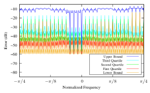
(a) Algorithm 1

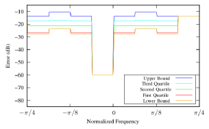
(b) Algorithm 2

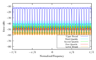
(c) Algorithm 3

Figure 3: Log-magnitude error of the frequency response of the rows of the proposed approximations. The errors are bounded to $-60$ dB for displaying purposes.

Note that the three approximations resulting from Algorithm 1, Algorithm 2, and Algorithm 3 have distinct frequency responses. Fig. 3 indicates that the Algorithm 1 is the one presenting the largest deviation for the main lobe from the exact DFT. This is expected given that the transform resulting from Algorithm 1 is obtained through the substitution of both the row- and column-wise DFT block by the discussed approximate 32-point DFT. This qualitative analysis is confirmed once we calculate the errors in the frequency responses of the rows of the three proposed approximations. Table 2 displays the minimum (nonzero), mean, and maximum for the squared magnitude of these errors. Notice in Fig. 3 that the transform resulting from Algorithm 1 has the highest deviations from the expected frequency response for its rows with range of $5$ dB compared to the filter bank response of the exact DFT matrix. In Table 2, we also show the worst-case side lobe in dB for each of the transforms. All transforms considered here possess a low worst-case side lobe on the order of $-12$ dB.

Noise rejection of the proposed ADFTs can be evaluated by means of its SNR improvement per frequency bin. The noise present from the antenna array can be modeled as additive white Gaussian noise (AWGN) with zero mean and variance $\sigma^{2}$. The AWGN present in each frequency bin is $\sigma^{2}/N.$ For narrowband (monochromatic) plane wave received by the array, the input signals to both the DFT and the three ADFT algorithms follows $\exp(j2\pi nk/N)$ for $n,k=0,1,\ldots,N-1$, where $k$ represents the DFT/ADFT bin number (corresponding to specific spatial frequencies related to the direction of propagation of each wave) and $n$ is the antenna number in the ULA. The monochromatic signal having frequency $\exp(j2\pi k/N)$ for bin $k$ has its SNR improved by $10\operatorname{log}_{10}(N)$, which is $30.1\leavevmode\nobreak\$dB for the 1024 point DFT. This is the best case SNR improvement per bin for the DFTs. The adoption of various ADFTs in place of the DFT causes a loss of SNR performance observed as a hit in the SNR per bin. Let the reduction in SNR for bin $k$ be denoted $\Delta\gamma_{x}$ where $x\in\{1,2,3\}$ are for the three proposed approximation algorithms.

The worst-case SNR degradation for the ADFTs obtained through simulations with $10^{5}$ replicates for finding the ensemble average for each bin of the ADFTs are shown in Table 2. The SNR degradation shows that Algorithm 1 has the largest worst-case degradation of SNR compared to the DFT ($\Delta\gamma_{1}<0.9\leavevmode\nobreak\$dB). There is no significant difference between Algorithm 2 and Algorithm 3 in terms of SNR degradation and has worst-case ($\Delta\gamma_{2,3}<0.4\leavevmode\nobreak\$dB). The reduction in SNR of the three ADFTs compared to SNR of DFTs can be compensated by adding $\leq 0.9\leavevmode\nobreak\$ dB of additional transmit power and antenna gain at the transmit side.

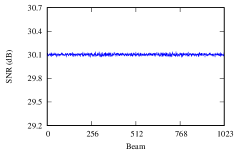
(a) DFT

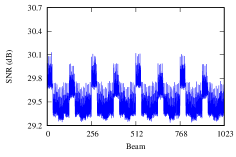
(b) Algorithm 1

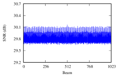
(c) Algorithm 2

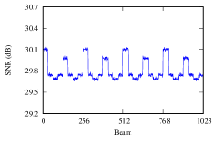
(d) Algorithm 3

Figure 4: The SNR for DFT and proposed Algorithm 1, Algorithm 2, and Algorithm 3. The SNR for the proposed algorithms is no lower than $29.2$ dB, against $30.1$ dB for the DFT.

Fig. 4 shows the SNR plot for each of the beams of the DFT and the three proposed approximations. Notice that no approximation has an SNR lower than $29.2$ dB in any of the bins, demonstrating that the SNR degradation is $\leq 0.9$ dB compared to the DFT where the SNR improves by $30.1$ dB for every bin.

Table 2: Performance statistics of the proposed approximations: frequency response magnitude, worst-case side lobe level and SNR degradation

Transform	Error Magnitude of Rows			Worst Side	SNR
	Min (dB)	Mean (dB)	Max (dB)	Lobe (dB )	degradation (dB)
Algorithm 1	$-10.7$	$-5.5$	$-4.4$	$-12.8$	$-0.6$
Algorithm 2	$-10.7$	$-9.9$	$-9.0$	$-12.8$	$-0.3$
Algorithm 3	$-10.7$	$-9.9$	$-9.0$	$-12.9$	$-0.3$

4 Digital VLSI Realization

Next, we explore digital VLSI realizations of the three ADFT approaches outlined in (20), (21) and (21) using a time-multiplexed approach. Traditionally, arithmetic complexity amounts of counts of both multiplication operations and addition operations. However, for semi-parallelized hardware implementations on VLSI platforms, the existence of parallel sub-systems offers a trade-off between circuit complexity and algorithm execution speed as described by Amdahl’s Law [3]. The proposed algorithms are based on radix-32 SFGs, which imply the sequential nature is limited to 1024-point algorithm completion every 32 clock cycles. The radix-32 SFG allows re-use of ADFT and DFT cores, and twiddle-factor cores, using time-multiplexing up to 32 levels. The use of time-multiplexed operations leads to the generalization of the multiplier structures that do not distinguish trivial multiplications by $0,1,-1.$ Therefore, the number of multiplications for the twiddle factor block is 1024 complex multiplications (compare to 961 complex multiplications for a sequential algorithm that can ignore trivial multiplications). However, radix-32 approach allows time-multiplexing of 32 parallel complex multipliers for achieving the twiddle factor matrix, leading to circuit complexity of 96 real multipliers, and 160 real adders/subtractors, in the twiddle factor block. To distinguish the mathematical operations from its physical realization, hereafter we refer to the circuit implementation of the selected 32-point DFT and ADFT, respectively, as DFT32 and ADFT32 cores. Also, the digital VLSI hardware for the 1024-point exact DFT and each of the 1024-point approximations resulting from Algorithm 1, Algorithm 2, and Algorithm 3 are referred to as the DFT1024, ADFT1024_1, ADFT1024_2, and ADFT1024_3 cores, respectively. Fig. 5 shows the overall architecture of the DFT1024 with the DFT32 cores. We focus on the design of the ADFT1024_1 core. Because this design can be easily extended to the other cores, the description of the ADFT1024_2 (Algorithm 2) and ADFT1024_3 (Algorithm 3) cores is omitted for brevity.

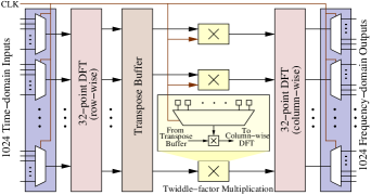
Figure 5: Signal flow graph showing the VLSI architecture to be modified for the proposed architecture based on the selected approximation. Algorithm 1: Replacement of both 32-point DFTs with 32-point ADFT blocks. Algorithm 2: Replacement of only row-wise 32-point DFT with 32-point ADFT blocks leaving column-wise DFT exact. Algorithm 3: Replacement of column-wise 32-point FFT with 32-point ADFT blocks leaving row-wise DFT exact.

The core ADFT1024_1 is a radix-32 unit and therefore processes an input signal block of 1024 time-domain samples in 32 clock cycles. Each signal block consists of 32 rows of adjacent time-domain samples in 32 columns. The first ADFT32 block sequentially computes the 32-point ADFT of each row, which are given by: $x[k],x[32+k],x[2\times 32+k],\ldots,x[31\times 32+k]$, for $k=0,1,\ldots,31$. Sampled values in the intermediate frequency (IF) domain are passed to the transpose buffer, which realizes the matrix transposition operation in digital VLSI hardware, while operating in-step with the system clock. One complete matrix transpose operation is achieved every 32 clock cycles. The transpose buffer feeds the second time-multiplexed ADFT32 after suitable twiddle factors have been applied, which in turn, furnishes the desired 1024-point ADFT values. In order to minimize the chances of overflow, the second time-multiplexed ADFT32 block in Fig. 5 uses a larger wordlength by one bit than the first time-multiplexed ADFT32 block. Use of a larger word length accommodates for the arithmetic operations that are carried on the first time-multiplexed ADFT32 and the twiddle factors.

4.1 Transpose Buffer and Twiddle Factors

The transpose buffer shown in Fig. 6 consists of a mesh of 1024 delays and 32 parallel multiplexers, each of them possessing 32 inputs. The transpose buffer block generates the transpose of the first set of frequency bins. The transposition allows the column-wise DFT computation required in eq. (20), (21) and (22).

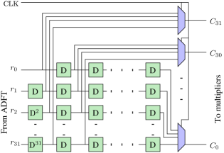
Figure 6: Schematic diagram of the transpose buffer.

Twiddle-factor multiplication count consists of 961 non-trivial complex multiplications spread over 32 clock cycles. However, these are implemented using 32 parallel complex multipliers, which each consume 3 real multipliers and 5 adders (Gauss Algorithm for complex multiplication). The twiddle factor block therefore furnishes the only multiplications present in ADFT1024_1, which results from Algorithm 1 in a radix-32 hardware realization. Each of the column bins (after the transpose buffer) undergoes a multiplication by $\omega_{1024}^{m\cdot n}$, where $0\leq m\leq 31$ and $0\leq n\leq 31$.

Therefore, the precision of the twiddle-factor multipliers plays a critical role in the final area $A$, area-time $AT$, and area-time-squared ($AT^{2}$) metrics. In this paper, we have set the twiddle-factor precision level to be equal to the system word size of the inputs to the ADFT1024_1 core, which is a design parameter and the choice of lower precision levels in the twiddle factors would result in improvements in the VLSI metrics for all three proposed algorithms. In a sense, hardware designed with such conservative parameters can be thought of as worst-case benchmark, with more coarsely quantified twiddle factors leading to even better improvements in area, area-time, and area-time-squared metrics.

4.2 Circuit Complexity

All circuits operate for 32 clock cycles to produce one 1024-point transform. Complex multiplication is realized using 3 real multiplier circuits and 5 real adder circuits following the Gauss multiplication algorithm. The twiddle-factor matrix based on Gauss multiplication $\mathbf{\Omega}_{32}$ in (20) therefore requires 96 real multiplier circuits and 160 adders circuits. This block is common to all four 1024-point algorithms.

4.2.1 ADFT1024_1 core

Each ADFT32 requires 348 adders/subtractors and no multipliers.

As shown in Fig. 5, the proposed radix-32 time-multiplexed architecture for Algorithm 1 uses two ADFT32 cores. Thus, ADFT1024_1 has an overall circuit complexity of $348*2+160=856$ adders/subtractor circuits and $96$ real multiplier circuits.

4.2.2 ADFT1024_2 core

In ADFT1024_2, the row-wise DFT block is substituted by the ADFT32 block. The DFT32 requires a total $78$ real multiplier circuits and $398$ adder circuits. Because the ADFT32 requires $348$ adder circuits but no multipliers, we have an overall circuit complexity of $398+160+348=906$ adder circuits and $96+78=174$ multipliers ADFT1024_2.

4.2.3 ADFT1024_3 core

The circuit complexity for the Algorithm 3 is the same as for ADFT1024_2. The only change is in the placement of the elements in the architectural level.

The 1024-point DFT (denoted DFT1024) obtained by using two DFT32 cores for row- and column-wise FFTs would require $78*2+96=252$ real multiplier circuits and $398*2+160=796+160=956$ adder circuits. This is our reference radix-32 FFT circuit for baselining the circuit complexities of the proposed ADFT1024 algorithms.

The circuit complexities for the proposed designs as well as DFT1024 are presented in Table 3.

Table 3: Circuit complexity for the proposed architectures and the 1024-point DFT

Design	Multiplier Circuits	Adder Circuits
$DFT1024$	$252$	$959$
$ADFT1024\_1$	$96$	$856$
$ADFT1024\_2$	$174$	$906$
$ADFT1024\_3$	$174$	$906$

4.3 ASIC Synthesis and Place-Route Results: 45nm CMOS

The proposed architectures were implemented on MATLAB Simulink using Xilinx libraries and then mapped to 45-nm complementary metal-oxide semiconductor (CMOS) technology cells (synthesis only). Each of the designs consists of three main hardware components—first 32-point transform block, transpose buffer with twiddle-factor multiplication block, and second 32-point transform block. The complexity of each 32-point transform block core depends on its corresponding input word length. Key quantitative measurements of performance for each 32-point transform block core and transpose buffer with twiddle-factor multiplications are shown in Table 4. In Table 5, we list the hardware implementation metrics for ADFT1024_1, ADFT1024_2, and ADFT1024_3. Metrics for the DFT1024 core were included as reference values.

Table 4: Key quantitative measurements of performance in digital 45 nm CMOS VLSI for each DFT core and transpose buffer with twiddle factor multiplications

Performance Metric	Row-wise transform			Transpose buffer with multipliers	Column-wise transform
	DFT32	ADFT32	Change		DFT32	ADFT32	Change
Area, $A$ (mm${}^{2})$	4.4	1.0	76.9 $\%\downarrow$	6.9	6.8	1.5	78.4 $\%\downarrow$
Critical Path Delay, $T$ (ns)	1.9	1.8	3.1 $\%\downarrow$	1.8	1.9	1.8	3.1 $\%\downarrow$
Frequency, $F_{\text{max}}$ (GHz)	0.5	0.6	3.2 $\%\uparrow$	0.6	0.5	0.6	3.2 $\%\uparrow$
$AT$ (mm2ns)	8.3	1.9	77.7 $\%\downarrow$	12.6	12.9	2.7	79.1 $\%\downarrow$
$AT^{2}$ (mm2ns2)	15.7	3.4	78.4 $\%\downarrow$	22.9	24.2	4.9	79.8 $\%\downarrow$
Dynamic Power, $D_{p}$ (mW/GHz)	10.1	2.0	80.1 $\%\downarrow$	10.4	24.3	2.8	88.5 $\%\downarrow$

Table 5: Key quantitative measurements of performance in digital 45 nm CMOS VLSI for each algorithm

Performance Metric	DFT1024	ADFT1024_1		ADFT1024_2		ADFT1024_3
		Value	Change	Value	Change	Value	Change
Area, $A$ (mm2)	18.2	9.4	48.3$\%\downarrow$	14.8	18.8$\%\downarrow$	12.8	29.5$\%\downarrow$
Critical Path Delay, $T$ (ns)	1.9	1.8	3.1$\%\downarrow$	1.9	-	1.9	-
Frequency, $F_{\text{max}}$ (GHz)	0.5	0.6	3.2$\%\uparrow$	0.5	-	0.5	-
$AT$ (mm2ns)	34.2	17.1	49.9$\%\downarrow$	27.8	18.8$\%\downarrow$	24.1	29.5$\%\downarrow$
$AT^{2}$ (mm2ns2)	64.3	31.2	51.5$\%\downarrow$	52.3	18.8$\%\downarrow$	45.4	29.5$\%\downarrow$
Dynamic Power, $D_{p}$ (mW/GHz)	44.8	15.2	66.0$\%\downarrow$	36.7	18.0$\%\downarrow$	23.3	48.0$\%\downarrow$

4.4 Analysis of the Results

The results in Table 4 shows that the 32-point ADFT core demands considerably less hardware resources than the 32-point exact DFT core. On the other hand, the implementation of the transpose buffer with twiddle factor multiplication adds a fixed hardware complexity to the system for both the DFT and the approximate architectures. As a result, the transpose buffer causes the highest area consumption and a relatively high power consumption in comparison to that of 32-point ADFT cores. Thus, it becomes the dominant factor in hardware complexity for the designs of the three 1024-point approximate transforms, as shown in Table 5.

The core ADFT1024_1 gives the best hardware utilization, whereas ADFT1024_2 gives the worst as can be seen in Table 5. Algorithm 3 gives the best error performance, i.e., provides the most accurate approximation. Moreover, the hardware resource consumption of its physical realization ADFT1024_3 is also close to that of ADFT1024_2. The error performance of Algorithm 2 does not differ much from that of Algorithm 1, which also provides a hardware realization ADFT1024_1 with the lowest resource consumption. Therefore, we recommend either Algorithm 1 or Algorithm 3 (i.e., its hardware realizations ADFT1024_1 and ADFT1024_3) as the best designs.

4.5 ADFT-based 1024-Beam Digital Beamformers

In the proposed system, each ADFT bin corresponds to a unique direction in space. Ideally these bins should be identical to the spatial DFT bins, but their magnitude could deviate because of the approximation. The four worst bins for each of the three algorithms are shown in Fig. 7. The resulting errors are small enough to be acceptable for the low SNR scenarios seen in practical wireless systems.

Fig. 8 shows detailed plots of 4 consecutive beams (from bins 200-203) for the three proposed algorithms, together with the errors. We chose these four beams arbitrarily to showcase the shapes of the obtained RF beams in sufficient detail.

Note that practical realization of 1024-element ULAs for generating narrow ADFT-based beams in currently-licensed frequency bands (upto the V band) may be challenging due to the large sizes of the resulting apertures. However, due to ongoing research in the sub-THz range [20, 51, 26, 38, 11, 36, 23, 31, 8], the W and G bands will soon be commercially available for both licensed and unlicensed use. At a carrier frequency of 300 GHz, $\lambda/2=0.5$ mm and thus the size of a Nyquist-spaced 1024-element ULA would decrease to a reasonable value of 51.2 cm.

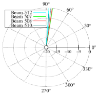
(a) DFT

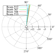
(b) Algorithm 1

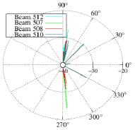
(c) Error for Algorithm 1

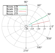
(d) DFT

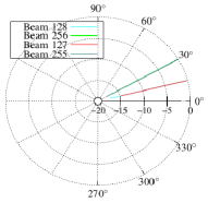
(e) Algorithm 2

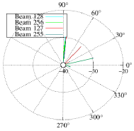
(f) Error for Algorithm 2

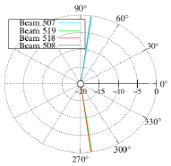
(g) DFT

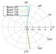
(h) Algorithm 3

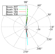
(i) Error for Algorithm 3

Figure 7: The four worst bins for multi-beam beamforming: (a) exact DFT response, (b) ADFT response, and (c) error for algorithm 1; (d) exact DFT response, (e) ADFT response, and (f) error for algorithm 2; (g) exact DFT response, (h) ADFT response, and (i) error for algorithm 3.

(a) DFT

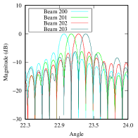
(b) Algorithm 1

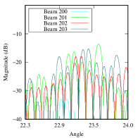
(c) Error for Algorithm 1

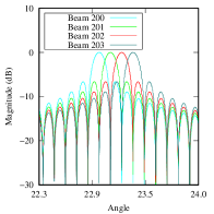
(d) Algorithm 2

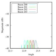
(e) Error for Algorithm 2

(f) Algorithm 3

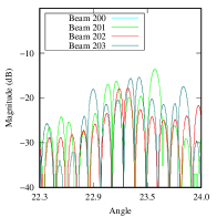
(g) Error for Algorithm 3

Figure 8: Linear plot of selected beams $\{200,201,202,203\}$ for exact and approximate transforms: (a) exact DFT response, (b) ADFT response, and (c) error for algorithm 1; (d) ADFT response, and (e) error for algorithm 2; (f) ADFT response, and (g) error for algorithm 3.

5 Conclusions

FFTs are used for reducing the computational costs of evaluating the DFT. Generally, they decrease complexity from $\mathcal{O}(N^{2})$ down to $\mathcal{O}(N\log N)$. In this paper, we show that further savings can be accomplished by means of approximate methods. The resulting 1024-point DFT approximations present a trade-off between performance and hardware complexity without significant loss in terms of worst-side lobe and SNR.

Our work shows that larger block-length DFT approximations can be obtained from the smaller-size approximations derived using previously-described numerical optimization methods. Our methodology can be directly applied to any DFT for which the block length is a perfect square. Since the current DFT approximations in the literature are restricted to the sizes $\{8,16,32\}$ [4, 15, 5, 24, 40], approximate algorithms can be derived for $N\in\{64,256,1024\}$. In this work, we focused on the 1024-point case. Assuming that a multiplierless DFT approximation of size $\sqrt{N}$ can always be found, our derivations suggests that we can obtain an $N$-point DFT approximation that requires only $N-2\sqrt{N}-1$ multiplications; effectively making the complexity of the resulting $N$-point approximation $\mathcal{O}(N)$. The proposed algorithms were synthesized to digital VLSI using a 45-nm CMOS library. Synthesis results confirm the expected improvements in layout area and power consumption metrics compared to a conventional 1024-point DFT implementation.

The choice of algorithm depends on the application and its tolerance for computational error in the DFT block. Highly error tolerant applications can greatly benefit from Algorithm 1 which has the lowest complexity. Algorithm 2 or 3 maybe selected when Algorithm 1 does not furnish sufficient performance.

References

[1]Technology blog.
IEEE Communication Society.
[2]A. Adhikary, J. Nam, J. Ahn, and G. Caire, Joint spatial
division and multiplexing–the large-scale array regime, IEEE Transactions
on Information Theory, 59 (2013), pp. 6441–6463.
[3]G. M. Amdahl, Validity of the single processor approach to achieving
large scale computing capabilities, in Proceedings of the April 18-20, 1967,
Spring Joint Computer Conference, AFIPS ’67 (Spring), New York, NY, USA,
1967, ACM, pp. 483–485.
[4]V. Ariyarathna, D. F. G. Coelho, S. Pulipati, R. J. Cintra, F. M.
Bayer, V. S. Dimitrov, and A. Madanayake, Multibeam digital array
receiver using a 16-point multiplierless DFT approximation, IEEE
Transactions on Antennas and Propagation, 67 (2019), pp. 925–933.
[5]V. Ariyarathna, S. Kulasekera, A. Madanayake, K. Lee, D. Suarez,
R. J. Cintra, F. M. Bayer, and L. Belostotski, Multi-beam 4 GHz
microwave apertures using current-mode DFT approximation on 65 nm CMOS,
in 2015 IEEE MTT-S International Microwave Symposium, May 2015, pp. 1–4.
[6]V. Ariyarathna, A. Madanayake, X. Tang, D. Coelho, R. J. Cintra,
L. Belostotski, S. Mandal, and T. S. Rappaport, Analog
approximate-FFT 8/16-beam algorithms, architectures and CMOS circuits for
5G beamforming MIMO transceivers, IEEE Journal on Emerging and Selected
Topics in Circuits and Systems, 8 (2018), pp. 466–479.
[7]T. Ayhan, W. Dehaene, and M. Verhelst, A 128:2048/1536 point FFT
hardware implementation with output pruning, in 22nd European Signal
Processing Conference (EUSIPCO), Sep. 2014, pp. 266–270.
[8]A. Babakhani, X. Guan, A. Komijani, A. Natarajan, and
A. Hajimiri, A 77-GHz phased-array transceiver with on-chip
antennas in silicon: Receiver and antennas, IEEE Journal of Solid-State
Circuits, 41 (2006), pp. 2795–2806.
[9]E. Bjornson, L. Sanguinetti, H. Wymeersch, J. Hoydis, and T. L. Marzetta,
Massive MIMO is a reality–what is next?: Five promising research
directions for antenna arrays, Digital Signal Processing, 94 (2019), pp. 3
– 20.
Special Issue on Source Localization in Massive MIMO.
[10]R. E. Blahut, Fast Algorithms for Signal Processing, Cambridge
University Press, 2010.
[11]S. Carpenter, Z. S. He, and H. Zirath, Balanced active
frequency multipliers in D and G bands using 250nm InP DHBT
technology, in IEEE Compound Semiconductor Integrated Circuit Symposium
(CSICS), Oct 2017, pp. 1–4.
[12]D. C. Champeney, A Handbook of Fourier Theorems, Cambridge
University Press, 1987.
[13]J. O. Coleman, A generalized FFT for many simultaneous receive
beams, tech. rep., Naval Research Lab, Washington DC - Signal Processing
Section, 2007.
[14]J. W. Cooley and J. W. Tukey, An algorithm for the machine
calculation of complex Fourier series, Mathematics of Computation, 19
(1965), pp. 297–301.
[15]V. A. Coutinho, V. Ariyarathna, D. F. G. Coelho, R. J. Cintral,
and A. Madanayake, An 8-beam 2.4 GHz digital array receiver based
on a fast multiplierless spatial DFT approximation, in 2018 IEEE/MTT-S
International Microwave Symposium - IMS, June 2018, pp. 1538–1541.
[16]P. Duhamel and H. Hollmann, Split radix FFT algorithm,
Electronics Letters, 20 (1984), pp. 14–16.
[17]T. Duong, vec, vech, invvec, invvech, 2019.
[18]S. W. Ellingson and W. Cazemier, Efficient multibeam synthesis with
interference nulling for large arrays, IEEE Transactions on Antennas and
Propagation, 51 (2003), pp. 503–511.
[19]M. T. Heideman, Multiplicative complexity of linear and bilinear
systems, in Multiplicative Complexity, Convolution, and the DFT, Springer,
1988, pp. 5–26.
[20]M. Hossain, K. Nosaeva, B. Janke, N. Weimann, V. Krozer, and
W. Heinrich, A G-band high power frequency doubler in
transferred-substrate InP HBT technology, IEEE Microwave and Wireless
Components Letters, 26 (2016), pp. 49–51.
[21]S. G. Johnson and M. Frigo, A modified split-radix FFT with fewer
arithmetic operations, IEEE Transactions on Signal Processing, 55 (2007),
pp. 111–119.
[22]M. Z. A. Khan and S. Qadeer, A new variant of radix-4 FFT, in
13th International Conference on Wireless and Optical Communications Networks
(WOCN), July 2016, pp. 1–4.
[23]J. Kim and J. F. Buckwalter, Staggered gain for 100+ GHz
broadband amplifiers, IEEE Journal of Solid-State Circuits, 46 (2011),
pp. 1123–1136.
[24]S. Kulasekera, A. Madanayake, R. J. Cintra, D. Suarez, and F. M. Bayer,
Multi-beam receiver apertures using multiplierless 8-point approximate
DFT, in IEEE Radar Conference (RadarCon), 2015.
[25]C. V. Kumar and K. R. K. Sastry, Design and implementation of FFT
pruning algorithm on FPGA, in 7th International Conference on Cloud
Computing, Data Science Engineering - Confluence, Jan 2017, pp. 739–743.
[26]A. Kurdoghlian, H. Moyer, H. Sharifi, D. F. Brown, R. Nagele,
J. Tai, R. Bowen, M. Wetzel, R. Grabar, D. Santos, and
M. Micovic, First demonstration of broadband W-band and D-band
GaN MMICs for next generation communication systems, in 2017 IEEE MTT-S
International Microwave Symposium (IMS), June 2017, pp. 1126–1128.
[27]A. Madanayake, V. Ariyarathna, S. Madishetty, S. Pulipati, R. J. Cintra,
D. Coelho, R. Oliveira, F. Bayer, L. Belostotski, S. Mandal, and
T. Rappaport, Towards a low-SWaP 1024-beam digital array: A 32-beam
sub-system at 5.8 GHz, IEEE Transactions on Antennas & Propagation,
(2018).
[28]E. Marchand, H. Uchiyama, and F. Spindler, Pose estimation for
augmented reality: A hands-on survey, IEEE Transactions on Visualization and
Computer Graphics, 22 (2016), pp. 2633–2651.
[31]A. Natarajan, A. Komijani, X. Guan, A. Babakhani, and
A. Hajimiri, A 77-GHz phased-array transceiver with on-chip
antennas in silicon: Transmitter and local LO-path phase shifting, IEEE
Journal of Solid-State Circuits, 41 (2006), pp. 2807–2819.
[32]A. V. Oppenheim and R. W. Schafer, Discrete-time Signal Processing,
Prentice Hall, 3 ed., 2009.
[33]K. R. Rao and P. C. Yip, eds., The Transform and Data Compression
Handbook, Electrical Engineering & Applied Signal Processing Series, CRC
Press, 2000.
[34]T. S. Rappaport, S. Sun, R. Mayzus, H. Zhao, Y. Azar, K. Wang,
G. N. Wong, J. K. Schulz, M. Samimi, and F. Gutierrez, Millimeter wave mobile communications for 5G cellular: It will work!,
IEEE Access, 1 (2013), pp. 335–349.
[35]T. S. Rappaport, Y. Xing, O. Kanhere, S. Ju, A. Madanayake,
S. Mandal, A. Alkhateeb, and G. C. Trichopoulos, Wireless
communications and applications above 100 GHz: Opportunities and challenges
for 6G and beyond, IEEE Access, (2019), pp. 1–1.
[36]M. Rodwell, Z. Griffith, N. Parthasarathy, E. Lind, C. Sheldon,
S. R. Bank, U. Singisetti, M. Urteaga, K. Shinohara, R. Pierson,
and P. Rowell, Developing bipolar transistors for sub-mm-wave
amplifiers and next-generation (300 GHz) digital circuits, in 64th Device
Research Conference, June 2006, pp. 5–8.
[37]G. A. F. Seber, A Matrix Handbook for Statisticians, Wiley Series
in Probability and Statistics, John Wiley & Sons, Inc., Hoboken, NJ, 2008.
[38]W. Shaobing, G. Jianfeng, W. Weibo, and Z. Junyun, W-band
MMIC PA with ultrahigh power density in 100-nm AlGaN/GaN technology,
IEEE Transactions on Electron Devices, 63 (2016), pp. 3882–3886.
[39]D. Suarez, R. J. Cintra, F. M. Bayer, A. Sengupta, S. Kulasekera, and
A. Madanayake, Multi-beam RF aperture using multiplierless FFT
approximation, Electronics Letters, 50 (2014), pp. 1788–1790.
[40]D. M. Suárez Villagrán, Aproximações para a transformada
discreta de Fourier e aplicações em deteção e estimação,
Master’s thesis, Universidade Federal de Pernambuo, Recife, Brazil, 2015.
Advisors: R. J. Cintra and F. M. Bayer.
[41]S. Sun, T. S. Rappaport, R. W. Heath, A. Nix, and S. Rangan,
MIMO for millimeter-wave wireless communications: beamforming, spatial
multiplexing, or both?, IEEE Communications Magazine, 52 (2014),
pp. 110–121.
[42]A. Taha, M. Alrabeiah, and A. Alkhateeb, Enabling large intelligent
surfaces with compressive sensing and deep learning, 2019.
[43]S. Winograd, On computing the discrete Fourier transform,
Mathematics of computation, 32 (1978), pp. 175–199.
[44], On the
multiplicative complexity of the discrete Fourier transform, Advances in
Mathematics, 32 (1979), pp. 83–117.
[45]S. Winograd, Arithmetic Complexity of Computations, CBMS-NSF
Regional Conference Series in Applied Mathematics, 1980.
[46]H. Wymeersch, G. Seco-Granados, G. Destino, D. Dardari, and
F. Tufvesson, 5G mmwave positioning for vehicular networks, IEEE
Wireless Communications, 24 (2017), pp. 80–86.
[47]Y. Xing, O. Kanhere, S. Ju, and T. S. Rappaport, Indoor
wireless channel properties at millimeter wave and sub-terahertz
frequencies, in 2019 IEEE Global Communications Conference (GLOBECOM), Dec
2019, pp. 1–6.
[48]Y. Xing and T. S. Rappaport, Propagation measurement system and
approach at 140 GHz-moving to 6G and above 100 GHz, in 2018 IEEE
Global Communications Conference (GLOBECOM), Dec 2018, pp. 1–6.
[49]C. Yang, Y. Xie, L. Chen, H. Chen, and Y. Deng, Design of a
configurable fixed-point FFT processor, in IET International Radar
Conference 2015, Oct 2015, pp. 1–4.
[50]Z. Zhang, X. Wang, K. Long, A. V. Vasilakos, and L. Hanzo, Large-scale MIMO-based wireless backhaul in 5G networks, IEEE Wireless
Communications, 22 (2015), pp. 58–66.
[51]K. Zhou, J. Ding, C. Zhou, and W. Wu, -band dual-band
quasi-elliptical waveguide filter with flexibly allocated frequency and
bandwidth ratios, IEEE Microwave and Wireless Components Letters, 28 (2018),
pp. 206–208.