Contextual Bandits with Smooth Regret: Efficient Learning in Continuous Action Spaces

Abstract

Designing efficient general-purpose contextual bandit algorithms that work with large—or even continuous—action spaces would facilitate application to important scenarios such as information retrieval, recommendation systems, and continuous control. While obtaining standard regret guarantees can be hopeless, alternative regret notions have been proposed to tackle the large action setting. We propose a smooth regret notion for contextual bandits, which dominates previously proposed alternatives. We design a statistically and computationally efficient algorithm—for the proposed smooth regret—that works with general function approximation under standard supervised oracles. We also present an adaptive algorithm that automatically adapts to any smoothness level. Our algorithms can be used to recover the previous minimax/Pareto optimal guarantees under the standard regret, e.g., in bandit problems with multiple best arms and Lipschitz/Hölder bandits. We conduct large-scale empirical evaluations demonstrating the efficacy of our proposed algorithms.

1 Introduction

Contextual bandits concern the problem of sequential decision making with contextual information. Provably efficient contextual bandit algorithms have been proposed over the past decade (Langford and Zhang, 2007; Agarwal et al., 2014; Foster and Rakhlin, 2020; Simchi-Levi and Xu, 2021; Foster and Krishnamurthy, 2021). However, these developments only work in setting with a small number of actions, and their theoretical guarantees become vacuous when working with a large action space (Agarwal et al., 2012). The hardness result can be intuitively understood through a “needle in the haystack” construction: When good actions are extremely rare, identifying any good action demands trying almost all alternatives. This prevents naive direct application of contextual bandit algorithms to large action problems, e.g., in information retrieval, recommendation systems, and continuous control.

To bypass the hardness result, one approach is to assume structure on the model class. For example, in the standard linear contextual bandit (Auer, 2002; Chu et al., 2011; Abbasi-Yadkori et al., 2011), learning the $d$ components of the reward vector—rather than examining every single action—effectively guides the learner to the optimal action. Additional structural assumptions have been studied in the literature, e.g., linearly structured actions and general function approximation (Foster et al., 2020; Xu and Zeevi, 2020), Lipschitz/Hölder regression functions (Kleinberg, 2004; Hadiji, 2019), and convex functions (Lattimore, 2020). While these assumptions are fruitful theoretically, they might be violated in practice.

An alternative approach is to compete against a less demanding benchmark. Rather than competing against a policy that always plays the best action, one can compete against a policy that plays the best smoothed distribution over the actions: a smoothed distribution—by definition—cannot concentrate on the best actions when they are in fact rare. Thus, for the previously mentioned “needle in the haystack” construction, the benchmark is weak as well. This de-emphasizes such constructions and focuses algorithm design on scenarios where intuition suggests good solutions can be found without prohibitive statistical cost.

Contributions

We study large action space problems under an alternate notion of regret. Our first contribution is to propose a novel benchmark—the smooth regret—that formalizes the “no needle in the haystack” principle. We also show that our smooth regret dominates previously proposed regret notions along this line of work (Chaudhuri and Kalyanakrishnan, 2018; Krishnamurthy et al., 2020; Majzoubi et al., 2020), i.e., any regret guarantees with respect to the smooth regret automatically holds for these previously proposed regrets.

We design efficient algorithms that work with the smooth regret and general function classes. Our first proposed algorithm, SmoothIGW, works with any fixed smoothness level $h>0$, and is efficient—both statistically and computationally—whenever the learner has access to standard oracles: (i) an online regression oracle for supervised learning, and (ii) a simple sampling oracle over the action space. Statistically, SmoothIGW achieves $\sqrt{T/h}$-type regret for whatever action spaces; here ${1}/{h}$ should be viewed as the effective number of actions. Such guarantees can be verified to be minimax optimal when related back to the standard regret. Computationally, the guarantee is achieved with $O(1)$ operations with respect to oracles, which can be usually efficiently implemented in practice. Our second algorithm is a master algorithm which combines multiple SmoothIGW instances to compete against any unknown smoothness level. We show this master algorithm is Pareto optimal.

With our smooth regret and proposed algorithms, we exhibit guarantees under the standard regret in various scenarios, e.g., in problems with multiple best actions (Zhu and Nowak, 2020) and in problems when the expected payoff function satisfies structural assumptions such as Lipchitz/Hölder continuity (Kleinberg, 2004; Hadiji, 2019). Our algorithms are minimax/Pareto optimal when specialized to these settings.

1.1 Paper Organization

We introduce our smooth regret in Section 2, together with statistical and computational oracles upon which our algorithms are built. In Section 3, we present our algorithm SmoothIGW, which illustrates the core ideas of learning with smooth regret at any fixed smoothness level. Built upon SmoothIGW, in Section 4, we present a CORRAL-type of algorithm that can automatically adapt to any unknown smoothness level. In Section 5, we connect our proposed smooth regret to the standard regret over various scenarios. We present empirical results in Section 6, and close with a discussion in Section 7.

2 Problem Setting

We consider the following standard contextual bandit problems. At any time step $t\in[T]$, nature selects a context $x_{t}\in\mathcal{X}$ and a distribution over loss functions $\ell_{t}:\mathcal{A}\rightarrow[0,1]$ mapping from the (compact) action set $\mathcal{A}$ to a loss value in $[0,1]$. Conditioned on the context $x_{t}$, the loss function is stochastically generated, i.e., $\ell_{t}\sim{\mathbb{P}}_{\ell_{t}}(\cdot\mid x_{t})$. The learner selects an action $a_{t}\in\mathcal{A}$ based on the revealed context $x_{t}$, and obtains (only) the loss $\ell_{t}(a_{t})$ of the selected action. The learner has access to a set of measurable regression functions $\mathcal{F}\subseteq(\mathcal{X}\times\mathcal{A}\rightarrow[0,1])$ to predict the loss of any context-action pair. We make the following standard realizability assumption studied in the contextual bandit literature (Agarwal et al., 2012; Foster et al., 2018; Foster and Rakhlin, 2020; Simchi-Levi and Xu, 2021).

Assumption 1 (Realizability).

There exists a regression function $f^{\star}\in\mathcal{F}$ such that ${\mathbb{E}}[\ell_{t}(a)\mid x_{t}]=f^{\star}(x_{t},a)$ for any $a\in\mathcal{A}$ and across all $t\in[T]$.

The smooth regret

Let $(\mathcal{A},\Omega)$ be a measurable space of the action set and $\mu$ be a base probability measure over the actions. Let $\mathcal{Q}_{h}$ denote the set of probability measures such that, for any measure $Q\in\mathcal{Q}_{h}$, the following holds true: (i) $Q$ is absolutely continuous with respect to the base measure $\mu$, i.e., $Q\ll\mu$; and (ii) The Radon-Nikodym derivative of $Q$ with respect to $\mu$ is no larger than $\frac{1}{h}$, i.e., $\frac{dQ}{d\mu}\leq 1/h$. We call $\mathcal{Q}_{h}$ the set of smoothing kernels at smoothness level $h$, or simply put the set of $h$-smoothed kernels. For any context $x\in\mathcal{X}$, we denote by $\mathsf{Smooth}_{h}(x)$ the smallest loss incurred by any $h$-smoothed kernel, i.e.,

$$\mathsf{Smooth}_{h}(x)\vcentcolon=\inf_{Q\in\mathcal{Q}_{h}}{\mathbb{E}}_{a\sim Q}[f^{\star}(x,a)].$$

Rather than competing with $\operatorname*{arg\,min}_{a\in\mathcal{A}}f^{\star}(x,a)$—an impossible job in many cases—we take $\mathsf{Smooth}_{h}(x)$ as the benchmark and define the smooth regret as follows:

$$\mathrm{\mathbf{Reg}}_{\mathsf{CB},h}(T) \coloneqq{\mathbb{E}}\left[\sum_{t=1}^{T}f^{\star}(x_{t},a_{t})-\mathsf{Smooth}_{h}(x_{t})\right].$$ (1)

One important feature about the above definition is that the benchmark, i.e., $\mathsf{Smooth}_{h}(x_{t})$, automatically adapts to the context $x_{t}$: This gives the benchmark more power and makes it harder to compete against. In fact, our smooth regret dominates many existing regret measures with easier benchmarks. We provide some examples in the following.

• Chaudhuri and Kalyanakrishnan (2018) propose the quantile regret, which aims at competing with the lower $h$-quantile of the loss function, i.e., $v_{h}(x)\vcentcolon=\inf\{\zeta:\mu(a\in\mathcal{A}:f^{\star}(x,a)\leq\zeta)\geq h\}$. Consider $\mathcal{S}_{h}\vcentcolon=\{a\in\mathcal{A}:f^{\star}(x,a)\leq\nu_{h}(x)\}$ such that $\mu(\mathcal{S}_{h})\geq h$. Let $\macc@depth\char 1\relax\frozen@everymath{\macc@group}\macc@set@skewchar\macc@nested@a 111{Q}_{h}\vcentcolon=\mu|_{\mathcal{S}_{h}}/\mu(\mathcal{S}_{h})$ denote the (normalized) probability measure after restricting $\mu$ onto $\mathcal{S}_{h}$. Since $\macc@depth\char 1\relax\frozen@everymath{\macc@group}\macc@set@skewchar\macc@nested@a 111{Q}_{h}\in\mathcal{Q}_{h}$, we clearly have $\mathsf{Smooth}_{h}(x)\leq{\mathbb{E}}_{a\sim\macc@depth\char 1\relax\frozen@everymath{\macc@group}\macc@set@skewchar\macc@nested@a 111{Q}_{h}}[f^{\star}(x,a)]\leq\nu_{h}(x)$. Besides, the (original) quantile was only studied in the non-contextual case.

• Krishnamurthy et al. (2020) study a notion of regret that is smoothed in a different way: Their regret aims at competing with a known and fixed smoothing kernel (on top of a fixed policy set) with Radon-Nikodym derivative at most ${1}/{h}$. Our benchmark is clearly harder to compete against since we consider any smoothing kernel with Radon-Nikodym derivative at most ${1}/{h}$.

Besides being more competitive with respect to above benchmarks, smooth regret can also be naturally linked to the standard regret under various settings previously studied in the bandit literature, e.g., in the discrete case with multiple best arms (Zhu and Nowak, 2020) and in the continuous case with Lipschitz/Hölder continuous payoff functions (Kleinberg, 2004; Hadiji, 2019). We provide detailed discussion in Section 5.

2.1 Computational Oracles

The first step towards designing computationally efficient algorithms is to identify reasonable oracle models to access the sets of regression functions or actions. Otherwise, enumeration over regression functions or actions (both can be exponentially large) immediately invalidate the computational efficiency. We consider two common oracle models: a regression oracle and a sampling oracle.

The regression oracles

A fruitful approach to designing efficient contextual bandit algorithms is through reduction to supervised regression with the class $\mathcal{F}$ (Foster and Rakhlin, 2020; Simchi-Levi and Xu, 2021; Foster et al., 2020, 2021a). Following Foster and Rakhlin (2020), we assume that we have access to an online regression oracle $\mathrm{\mathbf{Alg}}_{\mathsf{Sq}}$, which is an algorithm for sequential predication under square loss. More specifically, the oracle operates in the following protocol: At each round $t\in[T]$, the oracle makes a prediction $\widehat{f}_{t}$, then receives context-action-loss tuple $(x_{t},a_{t},\ell_{t}(a_{t}))$. The goal of the oracle is to accurately predict the loss as a function of the context and action, and we evaluate its performance via the square loss $(\widehat{f}_{t}(x_{t},a_{t})-\ell_{t}(a_{t}))^{2}$. We measure the oracle’s cumulative performance through the square-loss regret to $\mathcal{F}$, which is formalized below.

Assumption 2.

The regression oracle $\mathrm{\mathbf{Alg}}_{\mathsf{Sq}}$ guarantees that, with probability at least $1-\delta$, for any (potentially adaptively chosen) sequence $\left\{(x_{t},a_{t},\ell_{t}(a_{t}))\right\}_{t=1}^{T}$,

$${\mathbb{E}}\Bigg{[}\sum_{t=1}^{T} \left(\widehat{f}_{t}(x_{t},a_{t})-\ell_{t}(a_{t})\right)^{2}-\inf_{f\in\mathcal{F}}\sum_{t=1}^{T}\left(f(x_{t},a_{t})-\ell_{t}(a_{t})\right)^{2}\Bigg{]}\leq\mathrm{\mathbf{Reg}}_{\mathsf{Sq}}(T,\delta),$$

for some (non-data-dependent) function $\mathrm{\mathbf{Reg}}_{\mathsf{Sq}}(T,\delta)$.

Sometimes it’s useful to consider a weighted regression oracle, where the square errors are weighted differently. It is shown in Foster et al. (2020) (Theorem 5 therein) that any regression oracle satisfies 2 can be used to generate a weighted regression oracle that satisfies the following assumption.

Assumption 3.

The regression oracle $\mathrm{\mathbf{Alg}}_{\mathsf{Sq}}$ guarantees that, with probability at least $1-\delta$, for any (potentially adaptively chosen) sequence $\left\{(w_{t},x_{t},a_{t},\ell_{t}(a_{t}))\right\}_{t=1}^{T}$,

$${\mathbb{E}}\Bigg{[}\sum_{t=1}^{T} w_{t}\left(\widehat{f}_{t}(x_{t},a_{t})-\ell_{t}(a_{t})\right)^{2}-\inf_{f\in\mathcal{F}}\sum_{t=1}^{T}w_{t}\left(f(x_{t},a_{t})-\ell_{t}(a_{t})\right)^{2}\Bigg{]}\leq{\mathbb{E}}\left[\max_{t\in[T]}w_{t}\right]\mathrm{\mathbf{Reg}}_{\mathsf{Sq}}(T,{\delta}),$$

for some (non-data-dependent) function $\mathrm{\mathbf{Reg}}_{\mathsf{Sq}}(T,\delta)$.

For either regression oracle, we let $\mathcal{T}_{\mathsf{Sq}}$ denote an upper bound on the time to (i) query the oracle’s estimator $\widehat{f}_{t}$ with context-action pair $(x_{t},a)$ and receive its predicated value $\widehat{f}_{t}(x_{t},a)\in[0,1]$; (ii) query the oracle’s estimator $\widehat{f}_{t}$ with context $x_{t}$ and receive its argmin action $\widehat{a}_{t}=\operatorname*{arg\,min}_{a\in\mathcal{A}}\widehat{f}_{t}(x_{t},a)$; and (iii) update the oracle with example $(x_{t},a_{t},r_{t}(a_{t}))$. We let $\mathcal{M}_{\mathsf{Sq}}$ denote the maximum memory used by the oracle throughout its execution.

Online regression is a well-studied problem, with known algorithms for many model classes (Foster and Rakhlin, 2020; Foster et al., 2020): including linear models (Hazan et al., 2007), generalized linear models (Kakade et al., 2011), non-parametric models (Gaillard and Gerchinovitz, 2015), and beyond. Using Vovk’s aggregation algorithm (Vovk, 1998), one can show that $\mathrm{\mathbf{Reg}}_{\mathsf{Sq}}(T,\delta)=O(\log(\lvert\mathcal{F}\rvert/\delta))$ for any finite set of regression functions $\mathcal{F}$, which is the canonical setting studied in contextual bandits (Langford and Zhang, 2007; Agarwal et al., 2012). In the following of this paper, we use abbreviation $\mathrm{\mathbf{Reg}}_{\mathsf{Sq}}(T)\vcentcolon=\mathrm{\mathbf{Reg}}_{\mathsf{Sq}}(T,T^{-1})$, and will keep the $\mathrm{\mathbf{Reg}}_{\mathsf{Sq}}(T)$ term in our regret bounds to accommodate for general set of regression functions.

The sampling oracles

In order to design algorithms that work with large/continuous action spaces, we assume access to a sampling oracle $\mathrm{\mathbf{Alg}}_{\mathsf{Sample}}$ to get access to the action space. In particular, the oracle $\mathrm{\mathbf{Alg}}_{\mathsf{Sample}}$ returns an action $a\sim\mu$ randomly drawn according to the base probability measure $\mu$ over the action space $\mathcal{A}$. We let $\mathcal{T}_{\mathsf{Sample}}$ denote a bound on the runtime of single query to the oracle; and let $\mathcal{M}_{\mathsf{Sample}}$ denote the maximum memory used by the oracle.

Representing the actions

We use $b_{\mathcal{A}}$ to denote the number of bits required to represent any action $a\in\mathcal{A}$, which scales with $O(\log\lvert\mathcal{A}\rvert)$ with a finite set of actions and $\widetilde{O}(d)$ for actions represented as vectors in ${\mathbb{R}}^{d}$. Tighter bounds are possible with additional structual assumptions. Since representing actions is a minimal assumption, we hide the dependence on $b_{\mathcal{A}}$ in big-$O$ notation for our runtime and memory analysis.

2.2 Additional Notation

We adopt non-asymptotic big-oh notation: For functions $f,g:\mathcal{Z}\to{\mathbb{R}}_{+}$, we write $f=O(g)$ (resp. $f=\Omega(g)$) if there exists a constant $C>0$ such that $f(z)\leq{}Cg(z)$ (resp. $f(z)\geq{}Cg(z)$) for all $z\in\mathcal{Z}$. We write $f=\widetilde{O}(g)$ if $f=O(g\cdot\mathrm{polylog}(T))$, $f=\widetilde{\Omega}(g)$ if $f=\Omega(g/\mathrm{polylog}(T))$. We use $\lesssim$ only in informal statements to highlight salient elements of an inequality.

For an integer $n\in\mathbb{N}$, we let $[n]$ denote the set $\{1,\dots,n\}$. For a set $\mathcal{Z}$, we let $\Delta(\mathcal{Z})$ denote the set of all Radon probability measures over $\mathcal{Z}$. We let $\operatorname{{unif}}(\mathcal{Z})$ denote the uniform distribution/measure over $\mathcal{Z}$. We let $\mathbb{I}_{z}\in\Delta(\mathcal{Z})$ denote the delta distribution on $z$.

3 Efficient Algorithm with Smooth Regret

We design an oracle-efficient (SmoothIGW, Algorithm 1) algorithm that achieves a $\sqrt{T}$-type regret under the smooth regret defined in Eq. 1. We focus on the case when the smoothness level $h>0$ is known in this section, and leave the design of adaptive algorithms in Section 4.

Algorithm 1 contains the pseudo code of our proposed SmoothIGW algorithm, which deploys a smoothed sampling distribution to balance exploration and exploitation. At each round $t\in[T]$, the learner observes the context $x_{t}$ from the environment and obtains the estimator $\widehat{f}_{t}$ from the regression oracle $\mathrm{\mathbf{Alg}}_{\mathsf{Sq}}$. It then constructs a sampling distribution $P_{t}$ by mixing a smoothed distribution constructed using the inverse gap weighting (IGW) technique (Abe and Long, 1999; Foster and Rakhlin, 2020) and a delta mass at the greedy action $\widehat{a}_{t}\vcentcolon=\operatorname*{arg\,min}_{a\in\mathcal{A}}\widehat{f}_{t}(x_{t},a)$. The algorithm samples an action $a_{t}\sim P_{t}$ and then update the regression oracle $\mathrm{\mathbf{Alg}}_{\mathsf{Sq}}$. The key innovation of the algorithm lies in the construction of the smoothed IGW distribution, which we explain in detail next.

Algorithm 1 SmoothIGW

0:  Exploration parameter $\gamma>0$, online regression oracle $\mathrm{\mathbf{Alg}}_{\mathsf{Sq}}$.

1:  for $t=1,2,\dots,T$ do

2:     Observe context $x_{t}$.

3:     Receive $\widehat{f}_{t}$ from regression oracle $\mathrm{\mathbf{Alg}}_{\mathsf{Sq}}$.

4:     Get $\widehat{a}_{t}\leftarrow\operatorname*{arg\,min}_{a\in\mathcal{A}}\widehat{f}_{t}(x_{t},a)$.

5:     Define

$$P_{t}\vcentcolon=M_{t}+(1-M_{t}(\mathcal{A}))\cdot\mathbb{I}_{\widehat{a}_{t}},$$ (2)

where $M_{t}$ is the measure defined in Eq. 4

6:     Sample $a_{t}\sim P_{t}$ and observe loss $\ell_{t}(a_{t})$. // This can be done efficiently via Algorithm 2.

7:     Update $\mathrm{\mathbf{Alg}}_{\mathsf{Sq}}$ with $(x_{t},a_{t},\ell_{t}(a_{t}))$

Smoothed variant of IGW

The IGW technique was previously used in the finite-action contextual bandit setting (Abe and Long, 1999; Foster and Rakhlin, 2020), which assigns a probability mass to every action $a\in\mathcal{A}$ inversely proportional to the estimated loss gap $(\widehat{f}(x,a)-\widehat{f}(x,\widehat{a}))$. To extend this strategy to continuous action spaces we leverage Radon-Nikodym derivatives. Fix any constant $\gamma>0$, we define a IGW-type function as

$$m_{t}(a)\vcentcolon=\frac{1}{1+h\gamma(\widehat{f}_{t}(x_{t},a)-\widehat{f}_{t}(x_{t},\widehat{a}_{t}))}.$$ (3)

For any $\omega\in\Omega$, we then define a new measure

$$M_{t}(\omega)\vcentcolon=\int_{a\in\omega}m_{t}(a)\,d\mu(a)$$ (4)

of the measurable action space $(\mathcal{A},\Omega)$, where $m(a)=\frac{dM}{d\mu}(a)$ serves as the Radon-Nikodym derivative between the new measure $M$ and the base measure $\mu$. Since $m_{t}(a)\leq 1$ by construction, we have $M_{t}(\mathcal{A})\leq 1$, i.e., $M_{t}$ is a sub-probability measure. SmoothIGW plays a probability measure $P_{t}\in\Delta(\mathcal{A})$ by mixing the sub-probability measure $M_{t}$ with a delta mass at the greedy action $\widehat{a}_{t}$, as in Eq. 2.

Algorithm 2 Rejection Sampling for IGW

0:  Sampling oracle $\mathrm{\mathbf{Alg}}_{\mathsf{Sample}}$, greedy action $\widehat{a}_{t}$, Radon-Nikodym derivative $m_{t}(a)$.

1:  Draw $a\sim\mu$ from sampling oracle $\mathrm{\mathbf{Alg}}_{\mathsf{Sample}}$.

2:  Sample $Z$ from a Bernoulli random distribution with mean $m_{t}(a)$.

3:  if $Z=1$ then

4:     Take action $a$.

5:  else

6:     Take action $\widehat{a}_{t}$.

Efficient sampling

We now discuss how to sample from the distribution of Eq. 2 using a single call to the sampling oracle, via rejection sampling. We first randomly sample an action $a\sim\mu$ from the sampling oracle $\mathrm{\mathbf{Alg}}_{\mathsf{Sample}}$ and with respect to the base measure $\mu$. We then compute $m_{t}(a)$ in Eq. 3 with two evaluation calls to $\widehat{f}_{t}$, one at $\widehat{f}_{t}(x_{t},{a})$ and the other at $\widehat{f}_{t}(x_{t},\widehat{a}_{t})$. Finally, we sample a random variable $Z$ from a Bernoulli distribution with expectation $m_{t}(a)$ and play either action $\widehat{a}_{t}$ or action $a$ depending upon the realization of $Z$. One can show that the sampling distribution described above coincides with the distribution defined in Eq. 2 (Proposition 1). We present the pseudo code for rejection sampling in Algorithm 2.

Proposition 1.

The sampling distribution generated from Algorithm 2 coincides with the sampling distribution defined in Eq. 2.

Proof of Proposition 1.

Let $\macc@depth\char 1\relax\frozen@everymath{\macc@group}\macc@set@skewchar\macc@nested@a 111{P}_{t}$ denote the sampling distribution achieved by Algorithm 2. For any $\omega\in\Omega$, if $\widehat{a}_{t}\notin\omega$, we have

$$\macc@depth\char 1\relax\frozen@everymath{\macc@group}\macc@set@skewchar\macc@nested@a 111{P}_{t}(\omega)=\int_{a\in\omega}m_{t}(a)\,d\mu(a)=M_{t}(\omega)$$

Now suppose that $\widehat{a}_{t}\in\omega$: Then the rejection probability, which equals ${\mathbb{E}}_{a\sim\mu}\left[1-m_{t}(a)\right]=1-M_{t}(\mathcal{A})$, will be added to the above expression. ∎

We now state the regret bound for SmoothIGW in the following.

Theorem 1.

Fix any smoothness level $h\in(0,1]$. With an appropriate choice for $\gamma>0$, Algorithm 1 ensures that

$$\mathrm{\mathbf{Reg}}_{\mathsf{CB},h}(T)\leq{\sqrt{4T\,\mathrm{\mathbf{Reg}}_{\mathsf{Sq}}(T)/h}},$$

with per-round runtime $O(\mathcal{T}_{\mathsf{Sq}}+\mathcal{T}_{\mathsf{Sample}})$ and maximum memory $O(\mathcal{M}_{\mathsf{Sq}}+\mathcal{M}_{\mathsf{Sample}})$.

Key features of Algorithm 1

Algorithm 1 achieves $\widetilde{O}(\sqrt{T/h})$ regret, which has no dependence on the number of actions. This suggests the Algorithm 1 can be used in large action spaces scenarios and only suffer regret scales with $1/h$: the effective number of actions considered for smooth regret. We next highlight the statistical and computational efficiencies of Algorithm 1.

• Statistical optimality. It’s not hard to prove a $\widetilde{\Omega}(\sqrt{T/h})$ lower bound for the smooth regret by relating it to the standard regret under a contextual bandit problem with finite actions: (i) the smooth regret and the standard regret coincides when $h={1}/{\lvert\mathcal{A}\rvert}$; and (ii) the standard regret admits lower bound $\widetilde{\Omega}(\sqrt{\lvert\mathcal{A}\rvert T})$ (Agarwal et al., 2012). In Section 5, we further relate our smooth regret guarantee to standard regret guarantee under other scenarios and recover the minimax bounds.

• Computational efficiency. Algorithm 1 is oracle-efficient and enjoys per-round runtime and maximum memory that scales linearly with oracle costs. To our knowledge, this leads to the first computationally efficient general-purpose algorithm that achieves a $\sqrt{T}$-type guarantee under smooth regret. The previously known efficient algorithm applies an $\varepsilon$-Greedy-type of strategy and thus only achieves a $T^{2/3}$-type regret (Majzoubi et al. (2020), and with respect to a weaker version of the smooth regret).

Proof sketch for Theorem 1

To analyze Algorithm 1, we follow a recipe introduced by Foster and Rakhlin (2020); Foster et al. (2020, 2021b) based on the Decision-Estimation Coefficient (DEC, adjusted to our setting), defined as $\mathsf{dec}_{\gamma}(\mathcal{F})\vcentcolon=\sup_{\widehat{f},x}\mathsf{dec}_{\gamma}(\mathcal{F};\widehat{f},x)$, where

$$\mathsf{dec}_{\gamma}(\mathcal{F};\widehat{f},x)\vcentcolon=\inf_{P\in\Delta(\mathcal{A})}\sup_{f^{\star}\in\mathcal{F}}{\mathbb{E}}_{a\sim P}\bigg{[}f^{\star}(x,a^{\star})-\mathsf{Smooth}_{h}(x)-\frac{\gamma}{4}\cdot\big{(}\widehat{f}(x,a)-f^{\star}(x,a)\big{)}^{2}\bigg{]}.$$ (5)

Foster and Rakhlin (2020); Foster et al. (2020, 2021b) consider a meta-algorithm which, at each round $t$, (i) computes $\widehat{f}_{t}$ by appealing to a regression oracle, (ii) computes a distribution $P_{t}\in\Delta(\mathcal{A})$ that solves the minimax problem in Eq. 5 with $x_{t}$ and $\widehat{f}_{t}$ plugged in, and (iii) chooses the action $a_{t}$ by sampling from this distribution. One can show that for any $\gamma>0$, this strategy enjoys the following regret bound:

$$\mathrm{\mathbf{Reg}}_{\mathsf{CB},h}(T)\lesssim T\cdot\mathsf{dec}_{\gamma}(\mathcal{F})+\gamma\cdot\mathrm{\mathbf{Reg}}_{\mathsf{Sq}}(T),$$ (6)

More generally, if one computes a distribution that does not solve Eq. 5 exactly, but instead certifies an upper bound on the DEC of the form $\mathsf{dec}_{\gamma}(\mathcal{F})\leq\macc@depth\char 1\relax\frozen@everymath{\macc@group}\macc@set@skewchar\macc@nested@a 111{}_{\gamma}(\mathcal{F})$, the same result holds with $\mathsf{dec}_{\gamma}(\mathcal{F})$ replaced by $\macc@depth\char 1\relax\frozen@everymath{\macc@group}\macc@set@skewchar\macc@nested@a 111{}_{\gamma}(\mathcal{F})$. Algorithm 1 is a special case of this meta-algorithm, so to bound the regret it suffices to show that the exploration strategy in the algorithm certifies a bound on the DEC.

By applying principles of convex conjugate, we show that the IGW-type distribution of Eq. 2 certifies $\mathsf{dec}_{\gamma}(\mathcal{F})\leq\frac{2}{h\gamma}$ for any set of regression functions $\mathcal{F}$ (Lemma 3, deferred to Section A.1). With this bound on DEC, We can then bound the first term in Eq. 6 by $O(\frac{T}{h\gamma})$ and optimally tune $\gamma$ in Eq. 6 to obtain the desired regret guarantee.

Deriving the bound on the DEC is one of our key technical contributions, where we simultaneous eliminate the dependence on both the function class and (cardinality of) the action set. Previous bounds on the DEC assume either a restricted function class $\mathcal{F}$ or a finite action set.

4 Adapting to Unknown Smoothness Parameters

Our results in Section 3 shows that, with a known $h$, one can achieve smooth regret proportional to $\sqrt{T/h}$ against the optimal smoothing kernel in $\mathcal{Q}_{h}$. The total loss achieved by the learner is the smooth regret plus the total loss suffered by playing the optimal smoothing kernel. One can notice that these two terms go into different directions: When $h$ gets smaller, the loss suffered by the optimal smoothing kernel gets smaller, yet the regret term gets larger. It is apriori unclear how to balance these terms, and therefore desirable to design algorithms that can automatically adapt to an unknown $h\in(0,1]$. Note it is sufficient to adapt to unknown $h\in[1/T,1]$, as the regret bound is vacuous for $h<1/T$. We provide such an algorithm in this section.

The CORRAL master algorithm

Our algorithm follows the standard master-base algorithm structure: We run multiple base algorithms with different configurations in parallel, and then use a master algorithm to conduct model selection on top of base algorithms. The goal of the master algorithm is to balance the regret among base algorithms and eventually achieve a performance that is “close” to the best base algorithm (whose identity is unknown). We use the classical CORRAL algorithm (Agarwal et al., 2017) as the master algorithm and initiate a collection of $B=\left\lceil\log T\right\rceil$ (modified) Algorithm 1 as base algorithms. More specifically, for $b=1,2,\dots,B$, each base algorithm is initialized with smoothness level $h_{b}=2^{-b}$. For any $h^{\star}\in[1/T,1]$, one can notice that there exists a base algorithm $i^{\star}$ that suits well to this (unknown) $h^{\star}$ in the sense that $h_{b^{\star}}\leq h^{\star}\leq 2h_{b^{\star}}$. The goal of the master algorithm is thus to adapt to the base algorithm indexed by $b^{\star}$.

We provide a brief description of the CORRAL master algorithm, and direct the reader to Agarwal et al. (2017) for more details. The master algorithm maintains a distribution $q_{t}\in\Delta([B])$ over base algorithms. At each round, the master algorithm sample a base algorithm $I_{t}\sim q_{t}$ and passes the context $x_{t}$, the sampling probability $q_{t,I_{t}}$ and parameter $\rho_{t,I_{t}}\coloneqq 1/\min_{i\leq t}q_{t,I_{t}}$ into the base algorithm $I_{t}$. The base algorithm $I_{t}$ then performs its learning process: it samples an arm $a_{t}$, observes its loss $\ell_{t}(a_{t,I_{t}})$, and then updates its internal state. The master algorithm is updated with respect to the importance-weighted loss $\frac{\ell_{t}(a_{t,I_{t}})}{q_{t,I_{t}}}$ and parameter $\rho_{t,I_{t}}$. In order to obtain theoretical guarantees, the base algorithms are required to be stable, which is defined as follows.

Definition 1.

Suppose the base algorithm indexed by $b$ satisfies—when implemented alone—regret guarantee $\mathrm{\mathbf{Reg}}_{\mathsf{CB},h_{b}}(T)\leq R_{b}(T)$ for some non-decreasing $R_{b}(T):{\mathbb{N}}_{+}\rightarrow{\mathbb{R}}_{+}$. Let $\mathrm{\mathbf{Reg}}_{\mathsf{Imp},h}$ denote the importance-weighted regret for base algorithm $b$, i.e.,

$$\mathrm{\mathbf{Reg}}_{\mathsf{Imp},h_{b}}(T)\vcentcolon={\mathbb{E}}\left[\sum_{t=1}^{T}\frac{\mathbbm{1}(I_{t}=b)}{q_{t,b}}(f^{\star}(x_{t},a_{t})-\mathsf{Smooth}_{h_{b}}(x_{t}))\right].$$

The base algorithm $b$ is called $(\alpha,R_{b}(T))$ stable if $\mathrm{\mathbf{Reg}}_{\mathsf{Imp},h_{b}}(T)\leq{\mathbb{E}}\left[\rho^{\alpha}_{T,b}\right]R_{b}(T)$.

A stable base algorithm

Our treatment is inspired by Foster et al. (2020). Let $(\tau_{1},\tau_{2},\ldots)\subseteq[T]$ denote the time steps when the base algorithm $b$ is invoked, i.e., when $I_{t}=b$. When invoked, the base algorithm receives $(x_{t},q_{t,b},\rho_{t,b})$ from the master algorithm. The base algorithm then sample from a distribution similar to Eq. 2 but with a customized learning rate $\gamma_{t,b}\vcentcolon=\sqrt{8T/(h_{b}\cdot\rho_{t,b}\cdot\mathrm{\mathbf{Reg}}_{\mathsf{Sq}}(T))}$. After observing the loss $\ell_{t}(a_{t,b})$, the base algorithm then updates the weighted regression oracle satisfying 3. Our modified algorithm is summarized in Algorithm 3.

Algorithm 3 Stable Base Algorithm (Index $b$)

0:  Weighted online regression oracle $\mathrm{\mathbf{Alg}}_{\mathsf{Sq}}$.

1:  Initialize weighted regression oracle $\mathrm{\mathbf{Alg}}_{\mathsf{Sq}}$.

2:  for $t\in(\tau_{1},\tau_{2},\ldots)$ do

3:     Receive context $x_{t}$, probability $q_{t,b}$ and parameter $\rho_{t,b}$ from the master algorithm.

4:     Receive $\widehat{f}_{t,b}$ from the weighted online regression oracle $\mathrm{\mathbf{Alg}}_{\mathsf{Sq}}$.

5:     Get $\widehat{a}_{t,b}\leftarrow\operatorname*{arg\,min}_{a\in\mathcal{A}}\widehat{f}_{t,b}(x_{t},a)$.

6:     Define $\gamma_{t,b}\vcentcolon=\sqrt{8T/(h_{b}\cdot\rho_{t,b}\cdot\mathrm{\mathbf{Reg}}_{\mathsf{Sq}}(T))}$ and $w_{t,b}\vcentcolon=\mathbbm{1}(I_{t}=b)\cdot\gamma_{t,b}/q_{t,b}$.

7:     Define $P_{t,b}\vcentcolon=M_{t,b}+(1-M_{t,b}(\mathcal{A}))\cdot\mathbb{I}_{\widehat{a}_{t,b}}$ according to Eq. 2 but with $\gamma_{t,b}$ defined above.

8:     Sample $a_{t,b}\sim P_{t,b}$ and observe loss $\ell_{t}(a_{t,b})$. // This can be done efficiently via Algorithm 2.

9:     Update the weighted regression oracle $\mathrm{\mathbf{Alg}}_{\mathsf{Sq}}$ with $(w_{t,b},x_{t},a_{t},\ell_{t}(a_{t,b}))$

Proposition 2.

For any $b\in[B]$, Algorithm 3 is $\left(\frac{1}{2},\sqrt{4T\,\mathrm{\mathbf{Reg}}_{\mathsf{Sq}}(T)/h_{b}}\right)$-stable, with per-round runtime $O(\mathcal{T}_{\mathsf{Sq}}+\mathcal{T}_{\mathsf{Sample}})$ and maximum memory $O(\mathcal{M}_{\mathsf{Sq}}+\mathcal{M}_{\mathsf{Sample}})$.

We now provide our model selection guarantees that adapt to unknown smoothness parameter $h\in(0,1]$. The result directly follows from combining the guarantee of CORRAL (Agarwal et al., 2017) and our stable base algorithms.

Theorem 2.

Fix learning rate $\eta\in(0,1]$, the CORRAL algorithm with Algorithm 3 as base algorithms guarantees that

$$\mathrm{\mathbf{Reg}}_{\mathsf{CB},h}(T)=\widetilde{O}\left(\frac{1}{\eta}+\frac{\eta\,T\,\mathrm{\mathbf{Reg}}_{\mathsf{Sq}}(T)}{h}\right),\forall h\in(0,1].$$

The CORRAL master algorithm has per-round runtime $\widetilde{O}(\mathcal{T}_{\mathsf{Sq}}+\mathcal{T}_{\mathsf{Sample}})$ and maximum memory $\widetilde{O}(\mathcal{M}_{\mathsf{Sq}}+\mathcal{M}_{\mathsf{Sample}})$.

Remark 1.

We keep the current form of Theorem 2 to better generalize to other settings, as explained in Section 5. With a slightly different analysis, we can recover the $\widetilde{O}(T^{\frac{1}{1+\beta}}h^{-\beta}\left(\log\left\lvert\mathcal{F}\right\rvert\right)^{\frac{\beta}{1+\beta}})$ guarantee for any $\beta\in[0,1]$, which is known to be Pareto optimal (Krishnamurthy et al., 2020). We provide the proofs for this result in Section B.2.1.

5 Extensions to Standard Regret

We extend our results to various settings under the standard regret guarantee, including the discrete case with multiple best arms, and the continuous case under Lipschitz/Hölder continuity. Our results not only recover previously known minimax/Pareto optimal guarantees, but also generalize existing results in various ways.

Although our guarantees are stated in terms of the smooth regret, they are naturally linked to the standard regret among various settings studied in this section. We thus primarily focus on the standard regret in this section. Let $a^{\star}_{t}\vcentcolon=\operatorname*{arg\,min}_{a\in\mathcal{A}}f^{\star}(x_{t},a)$ denote the best action under context $x_{t}$. The standard (expected) regret is defined as

$$\mathrm{\mathbf{Reg}}_{\mathsf{CB}}(T) \vcentcolon={\mathbb{E}}\left[\sum_{t=1}^{T}f^{\star}(x_{t},a_{t})-f^{\star}(x_{t},a^{\star}_{t})\right].$$

We focus on the canonical case with a finite set of regression functions $\mathcal{F}$ and consider $\mathrm{\mathbf{Reg}}_{\mathsf{Sq}}(\mathcal{F})=O(\log(\left\lvert\mathcal{F}\right\rvert T))$ (Vovk, 1998).

5.1 Discrete Case: Bandits with Multiple Best Arms

Zhu and Nowak (2020) study a non-contextual bandit problem with a large (discrete) action set $\mathcal{A}$ which might contain multiple best arms. More specifically, suppose there exists a subset of optimal arms $\mathcal{A}^{\star}\subseteq\mathcal{A}$ with cardinalities $\left\lvert\mathcal{A}^{\star}\right\rvert=K^{\star}$ and $\left\lvert\mathcal{A}\right\rvert=K$, the goal is to adapt to the effective number of arms $\frac{K}{K^{\star}}$ and minimize the standard regret. Note that one could have $\frac{K}{K^{\star}}\ll K$ when $K^{\star}$ is large.

Existing Results. Suppose $\frac{K}{K^{\star}}=\Theta(T^{\alpha})$ for some $\alpha\in[0,1]$. Zhu and Nowak (2020) shows that: (i) when $\alpha$ is known, the minimax regret is $\widetilde{\Theta}(T^{(1+\alpha)/2})$; and (ii) when $\alpha$ is unknown, the Pareto optimal regret can be described by $\widetilde{O}(\max\left\{T^{\beta},T^{1+\alpha-\beta}\right\})$ for any $\beta\in[0,1)$.

Our Generalizations. We extend the problem to the contextual setting: We use $\mathcal{A}^{\star}_{x_{t}}\subseteq\mathcal{A}$ to denote the subset of optimal arms with respect to context $x_{t}$, and analogously assume that $\inf_{x\in\mathcal{X}}\left\lvert\mathcal{A}^{\star}_{x}\right\rvert=K^{\star}$ and $\frac{K}{K^{\star}}=T^{\alpha}$.

Since $\frac{K^{\star}}{K}$ represents the proportion of actions that are optimal, by setting $h=\frac{K^{\star}}{K}=T^{-\alpha}$ (and under uniform measure), we can then relate the standard regret to the smooth regret, i.e., $\mathrm{\mathbf{Reg}}_{\mathsf{CB}}(T)=\mathrm{\mathbf{Reg}}_{\mathsf{CB},h}(T)$. In the case when $\alpha$ is known, Theorem 1 implies that $\mathrm{\mathbf{Reg}}_{\mathsf{CB}}(T)=O\big{(}T^{(1+\alpha)/2}\log^{1/2}(\left\lvert\mathcal{F}\right\rvert T)\big{)}$. In the case with unknown $\alpha$, by setting $\eta=T^{-\beta}$ in Theorem 2, we have

$$\mathrm{\mathbf{Reg}}_{\mathsf{CB}}(T)=O\big{(}\max(T^{\beta},T^{1+\alpha-\beta}\log(\left\lvert\mathcal{F}\right\rvert T))\big{)}.$$

These results generalize the known minimax/Pareto optimal results in Zhu and Nowak (2020) to the contextual bandit case, up to logarithmic factors.

5.2 Continuous Case: Lipschitz/Hölder Bandits

Kleinberg (2004); Hadiji (2019) study non-contextual bandit problems with (non-contextual) mean payoff functions $f^{\star}(a)$ satisfying Hölder continuity. More specifically, let $\mathcal{A}=[0,1]$ (with uniform measure) and $L,\alpha>0$ be some Hölder smoothness parameters, the assumption is that

$$\lvert f^{\star}(a)-f^{\star}(a^{\prime})\rvert\leq L\,\lvert a-a^{\prime}\rvert^{\alpha},$$

for any $a,a^{\prime}\in\mathcal{A}$. The goal is to adapt to provide standard regret guarantee that adapts to the smoothness parameters $L$ and $\alpha$.

Existing Results. In the case when $L,\alpha$ are known, Kleinberg (2004) shows that the minimax regret scales as $\Theta(L^{1/(2\alpha+1)}T^{(\alpha+1)/(2\alpha+1)})$; in the case with unknown $L,\alpha$, Hadiji (2019) shows that the Pareto optimal regret can be described by $\widetilde{O}\big{(}\max\{T^{\beta},L^{1/(1+\alpha)}T^{1-\frac{\alpha}{1+\alpha}\beta}\}\big{)}$ for any $\beta\in[\frac{1}{2},1]$.

Our Generalizations. We extend the setting to the contextual bandit case and make the following analogous Hölder continuity assumption, i.e.,

$$\lvert f^{\star}(x,a)-f^{\star}(x,a^{\prime})\rvert\leq L\,\lvert a-a^{\prime}\rvert^{\alpha},\quad\forall x\in\mathcal{X}.$$

We first divide the action set $\mathcal{A}=[0,1]$ into $B=\left\lceil 1/h\right\rceil$ consecutive intervals $\{I_{b}\}_{b=1}^{B}$ such that $I_{b}=[(b-1){h},{b}{h}]$. Let $b_{t}$ denote the index of the interval where the best action $a^{\star}_{t}\vcentcolon=\operatorname*{arg\,min}_{a\in\mathcal{A}}f^{\star}(x_{t},a)$ lies into, i.e., $a^{\star}_{t}\in I_{b_{t}}$. Our smooth regret (at level $h$) provides guarantees with respect to the smoothing kernel $\operatorname{{unif}}(I_{b_{t}})$. Since we have ${\mathbb{E}}_{a\sim\operatorname{{unif}}(I_{b_{t}})}[f^{\star}(x_{t},a)]\leq f^{\star}(x_{t},a^{\star}_{t})+Lh^{\alpha}$ under Hölder continuity, the following guarantee holds under the standard regret

$$\mathrm{\mathbf{Reg}}_{\mathsf{CB}}(T)\leq\mathrm{\mathbf{Reg}}_{\mathsf{CB},h}(T)+Lh^{\alpha}T.$$ (7)

When $L,\alpha$ are known, setting $h=\Theta\big{(}L^{-2/(2\alpha+1)}T^{-1/(2\alpha+1)}\log^{1/(2\alpha+1)}(\left\lvert\mathcal{F}\right\rvert T)\big{)}$ in Theorem 1 (together with Eq. 7) leads to regret guarantee $O\big{(}L^{1/(2\alpha+1)}T^{(\alpha+1)/(2\alpha+1)}\log^{(\alpha/(2\alpha+1)}(\left\lvert\mathcal{F}\right\rvert T)\big{)}$, which is nearly minimax optimal (Kleinberg, 2004). In the case when $L,\alpha$ are unknown, setting $\eta=T^{-\beta}$ in Theorem 2 (together with Eq. 7) leads to

$$\mathrm{\mathbf{Reg}}_{\mathsf{CB}}(T)=O\left(\max\left\{T^{\beta},L^{1/(1+2\alpha)}T^{1-\frac{\alpha}{1+\alpha}\beta}\log^{\alpha/(1+\alpha)}(\lvert\mathcal{F}\rvert T)\right\}\right),$$

which matches the Pareto frontier obtained in Hadiji (2019) up to logarithmic factors.

6 Experiments

In this section we compare our technique empirically with prior art from the bandit and contextual bandit literature. Code to reproduce these experiments is available at https://github.com/pmineiro/smoothcb.

6.1 Comparison with Bandit Prior Art

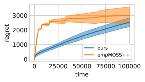
Figure 1: Comparison on a discrete action bandit dataset. Smaller is better. Following the display convention of Zhu and Nowak (2020), shaded areas are 38% confidence regions.

We replicate the real-world dataset experiment from Zhu and Nowak (2020). The dataset consists of 10025 captions from the New Yorker Magazine Cartoon Caption Contest and associated average ratings, normalized to [0, 1]. The caption text is discarded resulting in a non-contextual bandit problem with 10025 arms. When an arm is chosen, the algorithm experiences a Bernoulli loss realization whose mean is one minus the average rating for that arm. The goal is to experience minimum regret over the planning horizon $T=10^{5}$. There are 54 arms in the dataset that have the minimal mean loss of 0.

For our algorithm, we used the uniform distribution over $[1,2,\ldots,|\mathcal{A}|]$ as a reference measure, for which $O(1)$ sampling is available. We instantiated a tabular regression function, i.e., for each arm we maintained the empirical loss frequency observed for that arm. We use CORRAL with learning rate $\eta=1$ and instantiated 8 subalgorithms with $\gamma h$ geometrically evenly spaced between $10^{3}$ and $10^{6}$. These were our initial hyperparameter choices, but they worked well enough that no tuning was required.

In Fig. 1, we compare our technique with empMOSS++, the best performing technique from Zhu and Nowak (2020). Our technique is statistically equivalent.

6.2 Comparison with Contextual Bandit Prior Art

We replicate the online setting from Majzoubi et al. (2020), where 5 large-scale OpenML regression datasets are converted into continuous action problems on $[0,1]$ by shifting and scaling the target values into this range. The context $x$ is a mix of numerical and categorical variables depending upon the particular OpenML dataset. For any example, when the algorithm plays action $a$ and the true target is $y$, the algorithm experiences loss $|y-a|$ as bandit feedback.

We use Lebesgue measure on $[0,1]$ as our reference measure, for which $O(1)$ sampling is available. To maintain $O(1)$ computation, we consider regression functions with (learned) parameters $\theta$ via $f(x,a;\theta)\vcentcolon=g\left(\widehat{a}\left(x;\theta\right)-a;\theta\right)$ where, for any $\theta$, $z=0$ is a global minimizer of $g(z;\theta)$. Subject to this constraint, we are free to choose $g(\cdot;\theta)$ and $\widehat{a}(\cdot;\theta)$ and yet are ensured that we can directly compute the minimizer of our loss predictor via $\widehat{a}(x;\theta)$. For our experiments we use a logistic loss predictor and a linear argmin predictor with logistic link: Let $\theta\vcentcolon=(v;w;\xi)$, we choose

$$g(z;\theta)\vcentcolon=\sigma\left(|w||z|+\xi\right),\quad\text{and}\quad\widehat{a}(x;\theta)\vcentcolon=\sigma\left(v^{\top}x\right),$$

where $\sigma(\cdot)$ is the sigmoid function.

Table 1: Average progressive loss, scaled by 1000, on continuous action contextual bandit datasets. 95% bootstrap confidence intervals reported.

	CATS	Ours (Linear)	Ours (RFF)
Cpu	$[55,57]$	$[40.6,40.7]$	$\mathbb{[38.6,38.7]}$
Fri	$[183,187]$	$[161,163]$	$\mathbb{[156,157]}$
Price	$[108,110]$	$[70.2,70.5]$	$\mathbb{[66.1,66.3]}$
Wis	$[172,174]$	$[138,139]$	$\mathbb{[136.2,136.6]}$
Zur	$[24,26]$	$[24.3,24.4]$	$[25.4,25.5]$

In Table 1, we compare our technique with CATS from Majzoubi et al. (2020). Following their protocol, we tune hyperparameters for each dataset to be optimal in-hindsight, and then report 95% bootstrap confidence intervals based upon the progressive loss of a single run. Our algorithm outperforms CATS.

To further exhibit the generality of our technique, we also include results for a nonlinear argmin predictor in Table 1 (last column), which uses a Laplace kernel regressor implemented via random Fourier features (Rahimi et al., 2007) to predict the argmin. This approach achieves even better empirical performance.

7 Discussion

This work presents simple and practical algorithms for contextual bandits with large—or even continuous—action spaces, continuing a line of research which assumes actions that achieve low loss are not rare. While our approach can be used to recover minimax/Pareto optimal guarantees under certain structural assumptions (e.g., with Hölder/Lipschitz continuity), it doesn’t cover all cases. For instance, on a large but finite action set with a linear reward function, the optimal smoothing kernel can be made to perform arbitrarily worse than the optimal action (e.g., by having one optimal action lying in an orthogonal space of all other actions); in this construction, algorithms provided in this paper would perform poorly relative to specialized linear contextual bandit algorithms.

In future work we will focus on offline evaluation. Our technique already generates data that is suitable for subsequent offline evaluation of policies absolutely continuous with the reference measure, but only when the submeasure sample is accepted (line 4 of Algorithm 2), i.e., only $M(\mathcal{A})$ fraction of the data is suitable for reuse. We plan to refine our sampling distribution so that the fraction of re-usable data can be increased, but presumably at the cost of additional computation.

We manage to achieve a $\sqrt{T}$-regret guarantee with respect to smooth regret, which dominates previously studied regret notions that competing against easier benchmarks. A natural question to ask is, what is the strongest benchmark such that it is possible to still achieve a $\sqrt{T}$-type guarantee for problems with arbitrarily large action spaces? Speculating, there might exist a regret notion which dominates smooth regret yet still admits a $\sqrt{T}$ guarantee.

Appendix A Proofs and Supporting Results from Section 3

This section is organized as follows. We provide supporting results in Section A.1, then give the proof of Theorem 1 in Section A.2.

A.1 Supporting Results

A.1.1 Preliminaries

We first introduce the concept of convex conjugate. For any function $\phi:{\mathbb{R}}\rightarrow{\mathbb{R}}\cup\left\{-\infty,+\infty\right\}$, its convex conjugate $\phi^{\star}:{\mathbb{R}}\rightarrow{\mathbb{R}}\cup\left\{-\infty,+\infty\right\}$ is defined as

$$\phi^{\star}(w)\vcentcolon=\sup_{v\in{\mathbb{R}}}(vw-\phi(v)).$$

Since $(\phi^{\star})^{\star}=\phi$, we have (Young-Fenchel inequality)

$$\phi(v)\geq vw-\phi^{\star}(w),$$ (8)

for any $w\in\operatorname{{dom}}(\phi^{\star})$.

Lemma 1.

$\phi(v)=\frac{1}{\gamma}(v-1)^{2}$ and $\phi^{\star}(w)=w+\frac{\gamma}{4}w^{2}$ are convex conjugates.

Proof of Lemma 1.

By definition of the convex conjugate, we have

$$\phi^{\star}(w) =\sup_{v\in{\mathbb{R}}}\left(-\frac{1}{\gamma}\cdot\left(v^{2}-(2+\gamma w)v+1\right)\right)$$

$$=w+\frac{\gamma}{4}w^{2},$$

where the second line follows from plugging in the maximizer $v=\frac{\gamma w}{2}+1$. Note that the domain of $\phi^{\star}(w)$ is in fact ${\mathbb{R}}^{d}$ here. So, Eq. 8 holds for any $w\in{\mathbb{R}}^{d}$. ∎

We also introduce the concept of $\chi^{2}$ divergence. For probability measures $P$ and $Q$ on the same measurable space $(\mathcal{A},\Omega)$ such that $Q\ll P$, the $\chi^{2}$ divergence of $Q$ from $P$ is defined as

$$\chi^{2}(Q\;\|\;P)\vcentcolon={\mathbb{E}}_{a\sim P}\left[\left(\frac{dQ}{dP}(a)-1\right)^{2}\right],$$

where $\frac{dQ}{dP}(a)$ denotes the Radon-Nikodym derivative of $Q$ with respect to $P$, which is a function mapping from $a$ to ${\mathbb{R}}$.

A.1.2 Bounding the Decision-Estimation Coefficient

We aim at bounding the Decision-Estimation Coefficient in this section. We use expression $\inf_{Q\in\mathcal{Q}_{h}}{\mathbb{E}}_{a^{\star}\sim Q}[f^{\star}(x,a^{\star})]$ for $\mathsf{Smooth}_{h}(x)$. With this expression, we rewrite the Decision-Estimation Coefficient in the following: With respect to any context $x\in\mathcal{X}$ and estimator $\widehat{f}$ obtained from $\mathrm{\mathbf{Alg}}_{\mathsf{Sq}}$, we denote

$$\mathsf{dec}_{\gamma}(\mathcal{F};\widehat{f},x)\vcentcolon=\inf_{P\in\Delta(\mathcal{A})}\sup_{Q\in\mathcal{Q}_{h}}\sup_{f\in\mathcal{F}}{\mathbb{E}}_{a\sim P,a^{\star}\sim Q}\left[f(x,a)-f(x,a^{\star})-\frac{\gamma}{4}\cdot\left(\widehat{f}(x,a)-f(x,a)\right)^{2}\right],$$

and define $\mathsf{dec}_{\gamma}(\mathcal{F})\vcentcolon=\sup_{\widehat{f},x}\mathsf{dec}_{\gamma}(\mathcal{F};\widehat{f},x)$ as the Decision-Estimation Coefficient. We remark here that $\sup_{Q\in\mathcal{Q}_{h}}{\mathbb{E}}_{a^{\star}\sim Q}[-f(x,a^{\star})]=-\inf_{Q\in\mathcal{Q}_{h}}{\mathbb{E}}_{a\sim Q}[f^{\star}(x,a^{\star})]$ so we are still compete with the best smoothing kernel within $\mathcal{Q}_{h}$.

We first state a result that helps eliminate the unknown $f$ function in Decision-Estimation Coefficient (and thus the $\sup_{f\in\mathcal{F}}$ term), and bound Decision-Estimation Coefficient by the known $\widehat{f}$ estimator (from the regression oracle $\mathrm{\mathbf{Alg}}_{\mathsf{Sq}}$) and the $\chi^{2}$-divergence from $Q$ to $P$ (whenever $P$ and $Q$ are probability measures).

Lemma 2.

Fix constant $\gamma>0$ and context $x\in\mathcal{X}$ . For any measures $P$ and $Q$ such that $Q\ll P$, we have

$$\sup_{f\in\mathcal{F}}{\mathbb{E}}_{a\sim P,a^{\star}\sim Q}\left[f(x,a)-f(x,a^{\star})-\frac{\gamma}{4}\cdot\left(\widehat{f}(x,a)-f(x,a)\right)^{2}\right]$$

$$\leq{\mathbb{E}}_{a\sim P}\big{[}\widehat{f}(x,a)\big{]}-{\mathbb{E}}_{a\sim Q}\big{[}\widehat{f}(x,a)\big{]}+\frac{1}{\gamma}\cdot{\mathbb{E}}_{a\sim P}\left[\left(\frac{dQ}{dP}(a)-1\right)^{2}\right].$$

Proof of Lemma 2.

We omit the dependence on the context $x\in\mathcal{X}$, and use abbreviations $f(a)\vcentcolon=f(x,a)$ and $\widehat{f}(a)\vcentcolon=\widehat{f}(x,a)$. Let $g\vcentcolon=f-\widehat{f}$, we re-write the expression as

$$\sup_{f\in\mathcal{F}}{\mathbb{E}}_{a\sim P,a^{\star}\sim Q}\left[f(a)-f(a^{\star})-\frac{\gamma}{4}\cdot\left(\widehat{f}(a)-f(a)\right)^{2}\right]$$

$$=\sup_{g\in\mathcal{F}-\widehat{f}}{\mathbb{E}}_{a\sim P}\big{[}\widehat{f}(a)\big{]}-{\mathbb{E}}_{a^{\star}\sim Q}\big{[}\widehat{f}(a^{\star})\big{]}-{\mathbb{E}}_{a^{\star}\sim Q}\big{[}g(a^{\star})\big{]}+{\mathbb{E}}_{a\sim P}\left[g(a)-\frac{\gamma}{4}\cdot\left(g(a)\right)^{2}\right]$$

$$={\mathbb{E}}_{a\sim P}\big{[}\widehat{f}(a)\big{]}-{\mathbb{E}}_{a\sim Q}\big{[}\widehat{f}(a)\big{]}+\sup_{g\in\mathcal{F}-\widehat{f}}\left({\mathbb{E}}_{a\sim Q}\big{[}-g(a)\big{]}-{\mathbb{E}}_{a\sim P}\left[(-g(a))+\frac{\gamma}{4}\cdot\left(-g(a)\right)^{2}\right]\right)$$

$$={\mathbb{E}}_{a\sim P}\big{[}\widehat{f}(a)\big{]}-{\mathbb{E}}_{a\sim Q}\big{[}\widehat{f}(a)\big{]}+\sup_{g\in\mathcal{F}-\widehat{f}}{\mathbb{E}}_{a\sim P}\left[\frac{dQ}{dP}(a)\cdot(-g(a))-\left((-g(a))+\frac{\gamma}{4}\cdot\left(-g(a)\right)^{2}\right)\right]$$

$$={\mathbb{E}}_{a\sim P}\big{[}\widehat{f}(a)\big{]}-{\mathbb{E}}_{a\sim Q}\big{[}\widehat{f}(a)\big{]}+\sup_{g\in\mathcal{F}-\widehat{f}}{\mathbb{E}}_{a\sim P}\left[\frac{dQ}{dP}(a)\cdot(-g(a))-\phi^{\star}(-g(a))\right],$$

where we use the fact that $Q\ll P$ and $\phi^{\star}(w)=w+\frac{\gamma}{4}w^{2}$. Focus on the last term that depends on $g$ takes the form of the RHS of Eq. 8: Consider $v=\frac{dQ}{dP}(a)$ and $w=-g(a)$ and apply Eq. 8 (with Lemma 1) eliminates the dependence on $g$ (since it works for any $w=-g(a)$) and leads to the following bound

$$\sup_{f\in\mathcal{F}}{\mathbb{E}}_{a\sim P,a^{\star}\sim Q}\left[f(a)-f(a^{\star})-\frac{\gamma}{4}\cdot\left(\widehat{f}(a)-f(a)\right)^{2}\right]$$

$$\leq{\mathbb{E}}_{a\sim P}\big{[}\widehat{f}(a)\big{]}-{\mathbb{E}}_{a\sim Q}\big{[}\widehat{f}(a)\big{]}+\frac{1}{\gamma}\cdot{\mathbb{E}}_{a\sim P}\left[\left(\frac{dQ}{dP}(a)-1\right)^{2}\right].$$

∎

We now bound the Decision-Estimation Coefficient with sampling distribution defined in Eq. 2. We drop the dependence on $t$ and define the sampling distribution in the generic form: Fix any constant $\gamma>0$, context $x\in\mathcal{X}$ and estimator $\widehat{f}$, we define sampling distribution

$$P\vcentcolon=M+(1-M(\mathcal{A}))\cdot\mathbb{I}_{\widehat{a}},$$ (9)

where $\widehat{a}\vcentcolon=\operatorname*{arg\,min}_{a\in\mathcal{A}}\widehat{f}(x,a)$ and the measure $M$ is defined through $M(\omega)\vcentcolon=\int_{a\in\omega}m(a)\,d\mu(a)$ with

$$m(a)\vcentcolon=\frac{1}{1+h\gamma(\widehat{f}(x,a)-\widehat{f}(x,\widehat{a}))}.$$ (10)

Lemma 3.

Fix any constant $\gamma>0$ and any set of regression function $\mathcal{F}$. Let $P$ be the sampling distribution defined in Eq. 9, we then have $\mathsf{dec}_{\gamma}(\mathcal{F})\leq\frac{2}{h\,\gamma}$.

Proof of Lemma 3.

As in the proof of Lemma 2, we omit the dependence on the context $x\in\mathcal{X}$ and use abbreviations $f(a)\vcentcolon=f(x,a)$ and $\widehat{f}(a)\vcentcolon=\widehat{f}(x,a)$.

We first notice that for any $Q\in\mathcal{Q}_{h}$ we have $Q\ll M$ for $M$ defined in Eq. 10: we have (i) $Q\ll\mu$ by definition, and (ii) $\mu\ll M$ (since $m(a)\geq\frac{1}{1+h\gamma}>0$). On the other side, however, we do not necessarily have $P\ll\mu$ for $P$ defined in Eq. 9: It’s possible to have $P(\{a^{\star}\})>0$ yet $\mu(\{a^{\star}\})=0$, e.g., $\mu$ is some continuous measure. To isolate the corner case, we first give the following decomposition for any $Q\in\mathcal{Q}_{h}$ and $f\in\mathcal{F}$. With $P\vcentcolon=M+(1-M(\mathcal{A}))\cdot\mathbb{I}_{\widehat{a}}$, we have

$${\mathbb{E}}_{a\sim P,a^{\star}\sim Q}\left[f(a)-f(a^{\star})-\frac{\gamma}{4}\cdot\left(\widehat{f}(a)-f(a)\right)^{2}\right]$$

$$=(1-M(\mathcal{A}))\cdot\left(f(\widehat{a})-\frac{\gamma}{4}\cdot\big{(}\widehat{f}(\widehat{a})-f(\widehat{a})\big{)}^{2}\right)+{\mathbb{E}}_{a\sim M,a^{\star}\sim Q}\left[f(a)-f(a^{\star})-\frac{\gamma}{4}\cdot\left(\widehat{f}(a)-f(a)\right)^{2}\right]$$

$$=(1-M(\mathcal{A}))\cdot\left(\widehat{f}(\widehat{a})+\big{(}f(\widehat{a})-\widehat{f}(\widehat{a})\big{)}-\frac{\gamma}{4}\cdot\big{(}\widehat{f}(\widehat{a})-f(\widehat{a})\big{)}^{2}\right)+{\mathbb{E}}_{a\sim M,a^{\star}\sim Q}\left[f(a)-f(a^{\star})-\frac{\gamma}{4}\cdot\left(\widehat{f}(a)-f(a)\right)^{2}\right]$$

$$\leq(1-M(\mathcal{A}))\cdot\Big{(}\widehat{f}(\widehat{a})+\frac{1}{\gamma}\Big{)}+{\mathbb{E}}_{a\sim M,a^{\star}\sim Q}\left[f(a)-f(a^{\star})-\frac{\gamma}{4}\cdot\left(\widehat{f}(a)-f(a)\right)^{2}\right]$$

$$\leq\frac{1-M(\mathcal{A})}{\gamma}+(1-M(\mathcal{A}))\cdot{\widehat{f}(\widehat{a})}+{\mathbb{E}}_{a\sim M}\big{[}\widehat{f}(a)\big{]}-{\mathbb{E}}_{a\sim Q}\big{[}\widehat{f}(a)\big{]}+\frac{1}{\gamma}\cdot{\mathbb{E}}_{a\sim M}\left[\left(\frac{dQ}{dM}(a)-1\right)^{2}\right],$$ (11)

where the fourth line follows from applying AM-GM inequality and the fifth line follows from applying Lemma 2 with $Q\ll M$. We now focus on the last four terms in Eq. 11. Denote $m(a)\vcentcolon=\frac{dM}{d\mu}(a)$ and $q(a)\vcentcolon=\frac{dQ}{d\mu}(a)$, with change of measures, we have

$$(1-M(\mathcal{A})\cdot\big{(}\widehat{f}(\widehat{a})\big{)}+{\mathbb{E}}_{a\sim M}\big{[}\widehat{f}(a)\big{]}-{\mathbb{E}}_{a\sim Q}\big{[}\widehat{f}(a)\big{]}+\frac{1}{\gamma}\cdot{\mathbb{E}}_{a\sim M}\left[\left(\frac{dQ}{dM}(a)-1\right)^{2}\right]$$

$$={\mathbb{E}}_{a\sim\mu}\left[m(a)\cdot\Big{(}\widehat{f}(a)-\widehat{f}(\widehat{a})\Big{)}\right]-{\mathbb{E}}_{a\sim\mu}\left[q(a)\cdot\Big{(}\widehat{f}(a)-\widehat{f}(\widehat{a})\Big{)}\right]+\frac{1}{\gamma}\cdot{\mathbb{E}}_{a\sim\mu}\left[m(a)\cdot\left(\frac{q(a)}{m(a)}-1\right)^{2}\right]$$

$$={\mathbb{E}}_{a\sim\mu}\left[m(a)\cdot\Big{(}\widehat{f}(a)-\widehat{f}(\widehat{a})\Big{)}\right]-{\mathbb{E}}_{a\sim\mu}\left[q(a)\cdot\Big{(}\widehat{f}(a)-\widehat{f}(\widehat{a})\Big{)}\right]+\frac{1}{\gamma}\cdot{\mathbb{E}}_{a\sim\mu}\left[q(a)\cdot\frac{q(a)}{m(a)}-2q(a)+m(a)\right]$$

$$={\mathbb{E}}_{a\sim\mu}\left[m(a)\cdot\Big{(}\widehat{f}(a)-\widehat{f}(\widehat{a})\Big{)}\right]+\frac{1}{\gamma}\cdot{\mathbb{E}}_{a\sim Q}\left[\frac{q(a)}{m(a)}-\gamma\cdot\left(\widehat{f}(a)-\widehat{f}(\widehat{a})\right)\right]+\frac{M(\mathcal{A})-2}{\gamma}$$

Plugging LABEL:eq:prop_dec_bound_2 into Eq. 11 leads to

$${\mathbb{E}}_{a\sim P,a^{\star}\sim Q}\left[f(a)-f(a^{\star})-\frac{\gamma}{4}\cdot\left(\widehat{f}(a)-f(a)\right)^{2}\right]$$

$$\leq{\mathbb{E}}_{a\sim\mu}\left[m(a)\cdot\Big{(}\widehat{f}(a)-\widehat{f}(\widehat{a})\Big{)}\right]+\frac{1}{\gamma}\cdot{\mathbb{E}}_{a\sim Q}\left[\frac{q(a)}{m(a)}-\gamma\cdot\left(\widehat{f}(a)-\widehat{f}(\widehat{a})\right)\right]$$

$$\leq\frac{2}{h\gamma},$$ (13)

where Eq. 13 follows from the fact that $m(a)\vcentcolon=\frac{dM}{d\mu}(a)=\frac{1}{1+h\gamma(\widehat{f}(a)-\widehat{f}(\widehat{a}))}$ and $q(a)\vcentcolon=\frac{dQ}{d\mu}(a)\leq\frac{1}{h}$ for any $Q\in\mathcal{Q}_{h}$. This certifies that $\mathsf{dec}_{\gamma}(\mathcal{F})\leq\frac{2}{h\gamma}$. ∎

A.2 Proof of Theorem 1

See 1

Proof of Theorem 1.

We use abbreviation $f_{t}(a)\vcentcolon=f(x_{t},a)$ for any $f\in\mathcal{F}$. Let $a^{\star}_{t}$ denote the action sampled according to the best smoothing kernel within $\mathcal{Q}_{h}$ (which could change from round to round). We let $\mathcal{E}$ denote the good event where the regret guarantee stated in 2 (i.e., $\mathrm{\mathbf{Reg}}_{\mathsf{Sq}}(T)\vcentcolon=\mathrm{\mathbf{Reg}}_{\mathsf{Sq}}(T,T^{-1})$) holds with probability at least $1-T^{-1}$. Conditioned on this good event, following the analysis provided in Foster et al. (2020), we decompose the contextual bandit regret as follows.

$${\mathbb{E}}\left[\sum_{t=1}^{T}f_{t}^{\star}(a_{t})-f_{t}^{\star}(a^{\star}_{t})\right] ={\mathbb{E}}\left[\sum_{t=1}^{T}f_{t}^{\star}(a_{t})-f_{t}^{\star}(a^{\star}_{t})-\frac{\gamma}{4}\cdot\left(\widehat{f}_{t}(a_{t})-f_{t}^{\star}(a_{t})\right)^{2}\right]+\frac{\gamma}{4}\cdot{\mathbb{E}}\left[\sum_{t=1}^{T}\left(\widehat{f}_{t}(a_{t})-f_{t}^{\star}(a_{t})\right)^{2}\right]$$

$$\leq T\cdot\frac{2}{h\gamma}+\frac{\gamma}{4}\cdot{\mathbb{E}}\left[\sum_{t=1}^{T}\left(\widehat{f}_{t}(a_{t})-f_{t}^{\star}(a_{t})\right)^{2}\right],$$

where the bound on the first term follows from Lemma 3. We analyze the second term below.

$$\frac{\gamma}{4}\cdot{\mathbb{E}}\left[\sum_{t=1}^{T}\left(\left(\widehat{f}_{t}(a_{t})-\ell_{t}(a_{t})\right)^{2}-\Big{(}f^{\star}(a_{t})-\ell_{t}(a_{t})\Big{)}^{2}+2\Big{(}\ell_{t}(a_{t})-f^{\star}_{t}(a_{t})\Big{)}\cdot\Big{(}\widehat{f}_{t}(a_{t})-f^{\star}_{t}(a_{t})\Big{)}\right)\right]$$

$$=\frac{\gamma}{4}\cdot{\mathbb{E}}\left[\sum_{t=1}^{T}\left(\left(\widehat{f}_{t}(a_{t})-\ell_{t}(a_{t})\right)^{2}-\Big{(}f^{\star}_{t}(a_{t})-\ell_{t}(a_{t})\Big{)}^{2}\right)\right]$$

$$\leq\frac{\gamma}{4}\cdot\mathrm{\mathbf{Reg}}_{\mathsf{Sq}}(T),$$

where on the second line follows from the fact that ${\mathbb{E}}[\ell_{t}(a)\mid x_{t}]=f^{\star}(x_{t},a)$ and $\ell_{t}$ is conditionally independent of $a_{t}$, and the third line follows from the bound on regression oracle stated in 2. As a result, we have

$$\mathrm{\mathbf{Reg}}_{\mathsf{CB},h}(T)\leq\frac{2T}{h\gamma}+\frac{\gamma}{4}\cdot\mathrm{\mathbf{Reg}}_{\mathsf{Sq}}(T)+O(1),$$

where the additional term $O(1)$ accounts for the expected regret suffered under event $\neg\mathcal{E}$. Taking $\gamma=\sqrt{8T/(h\cdot\mathrm{\mathbf{Reg}}_{\mathsf{Sq}}(T))}$ leads to the desired result.

Computational complexity. We now discuss the computational complexity of Algorithm 1. At each round Algorithm 1 takes $O(1)$ calls to $\mathrm{\mathbf{Alg}}_{\mathsf{Sq}}$ to obtain estimator $\widehat{f}_{t}$ and the best action $\widehat{a}_{t}$. Instead of directly form the action distribution defined in Eq. 2, Algorithm 1 uses Algorithm 2 to sample action $a_{t}\sim P_{t}$, which takes one call of the sampling oracle $\mathrm{\mathbf{Alg}}_{\mathsf{Sample}}$ to draw a random action and $O(1)$ calls of the regression oracle $\mathrm{\mathbf{Alg}}_{\mathsf{Sq}}$ to compute the mean of the Bernoulli random variable. Altogether, Algorithm 1 has per-round runtime $O(\mathcal{T}_{\mathsf{Sq}}+\mathcal{T}_{\mathsf{Sample}})$ and maximum memory $O(\mathcal{M}_{\mathsf{Sq}}+\mathcal{M}_{\mathsf{Sample}})$. ∎

Appendix B Proofs from Section 4

This section is organized as follows. We first prove Proposition 2 in Section B.1, then prove Theorem 2 in Section B.2.

B.1 Proof of Proposition 2

The proof of Proposition 2 follows similar analysis as in Foster et al. (2020), with minor changes to adapt to our settings.

See 2

Proof of Proposition 2.

Fix the index $b\in[B]$ of the subroutine. We use shorthands $h=h_{b}$, $q_{t}=q_{t,b}$, $\rho_{t}=\rho_{t,b}$, $\gamma_{t}=\gamma_{t,b}$, and so forth. We also write $Z_{t}=Z_{t,b}\vcentcolon={\mathbbm{1}(I_{t}=b)}$. Similar to the proof of Theorem 1, we use abbreviation $f_{t}(a)\vcentcolon=f(x_{t},a)$ for any $f\in\mathcal{F}$. Let $a^{\star}_{t}$ denote the action sampled according to the best smoothing kernel within $\mathcal{Q}_{h}$ (which could change from round to round).

We let $\mathcal{E}$ denote the good event where the regret guarantee stated in 3 (with $\mathrm{\mathbf{Reg}}_{\mathsf{Sq}}(T)\vcentcolon=\mathrm{\mathbf{Reg}}_{\mathsf{Sq}}(T,T^{-1})$) holds with probability at least $1-T^{-1}$. Conditioned on this good event, similar to the proof of Theorem 1 (and following Foster et al. (2020)), we decompose the contextual bandit regret as follows.

$${\mathbb{E}}\left[\sum_{t=1}^{T}\frac{Z_{t}}{q_{t}}(f^{\star}_{t}(a_{t})-f_{t}^{\star}(a^{\star}_{t}))\right]$$

$$={\mathbb{E}}\left[\sum_{t=1}^{T}\frac{Z_{t}}{q_{t}}\left(f^{\star}_{t}(a_{t})-f_{t}^{\star}(a^{\star}_{t})-\frac{\gamma_{t}}{4}\cdot\left(\widehat{f}_{t}(a_{t})-f^{\star}_{t}(a_{t})\right)^{2}\right)\right]+{\mathbb{E}}\left[\sum_{t=1}^{T}\frac{Z_{t}}{q_{t}}\cdot\frac{\gamma_{t}}{4}\cdot\left(\widehat{f}_{t}(a_{t})-f^{\star}_{t}(a_{t})\right)^{2}\right]$$

$$\leq{\mathbb{E}}\left[\sum_{t=1}^{T}\frac{Z_{t}}{q_{t}}\cdot\frac{2}{h\gamma_{t}}\right]+{\mathbb{E}}\left[\sum_{t=1}^{T}\frac{Z_{t}}{q_{t}}\cdot\frac{\gamma_{t}}{4}\cdot\left(\widehat{f}_{t}(a_{t})-f^{\star}_{t}(a_{t})\right)^{2}\right]$$

$$\leq{\mathbb{E}}\left[\max_{t\in[T]}\gamma_{t}^{-1}\right]\cdot\frac{2T}{h}+{\mathbb{E}}\left[\sum_{t=1}^{T}\frac{Z_{t}}{q_{t}}\cdot\frac{\gamma_{t}}{4}\cdot\left(\widehat{f}_{t}(a_{t})-f^{\star}_{t}(a_{t})\right)^{2}\right],$$

where the bound on the first term follows from Lemma 3 (the third line, conditioned on $Z_{t}$). We bound the second term next.

$${\mathbb{E}}\left[\sum_{t=1}^{T}\frac{Z_{t}}{q_{t}}\cdot\frac{\gamma_{t}}{4}\cdot\left(\widehat{f}_{t}(a_{t})-f^{\star}_{t}(a_{t})\right)^{2}\right]$$

$$=\frac{1}{4}\cdot{\mathbb{E}}\left[\sum_{t=1}^{T}\frac{Z_{t}}{q_{t}}\gamma_{t}\left(\left(\widehat{f}_{t}(a_{t})-\ell_{t}(a_{t})\right)^{2}-\Big{(}f^{\star}_{t}(a_{t})-\ell_{t}(a_{t})\Big{)}^{2}+2\Big{(}\ell_{t}(a_{t})-f^{\star}_{t}(a_{t})\Big{)}\cdot\Big{(}\widehat{f}_{t}(a_{t})-f^{\star}_{t}(a_{t})\Big{)}\right)\right]$$

$$=\frac{1}{4}\cdot{\mathbb{E}}\left[\sum_{t=1}^{T}\frac{Z_{t}}{q_{t}}\gamma_{t}\left(\left(f_{t}(a_{t})-\ell_{t}(a_{t})\right)^{2}-\Big{(}f^{\star}_{t}(a_{t})-\ell_{t}(a_{t})\Big{)}^{2}\right)\right]$$

$$\leq\frac{1}{4}\cdot{\mathbb{E}}\left[\max_{t\in[T]}\frac{\gamma_{t}}{q_{t}}\right]\cdot\mathrm{\mathbf{Reg}}_{\mathsf{Sq}}(T),$$

where the last line follows from 3. As a result, we have

$$\mathrm{\mathbf{Reg}}_{\mathsf{Imp},h}(T)\leq{\mathbb{E}}\left[\max_{t\in[T]}\gamma_{t}^{-1}\right]\cdot\frac{2T}{h}+\frac{1}{4}\cdot{\mathbb{E}}\left[\max_{t\in[T]}\frac{\gamma_{t}}{q_{t}}\right]\cdot\mathrm{\mathbf{Reg}}_{\mathsf{Sq}}(T)+O(1),$$

where the additional $O(1)$ term is to account for the expected regret under event $\neg\mathcal{E}$. Notice that $\gamma_{t}\vcentcolon=\sqrt{8T/(h\cdot\rho_{t}\cdot\mathrm{\mathbf{Reg}}_{\mathsf{Sq}}(T))}$, which is non-increasing in $t$; and $\frac{\gamma_{t}}{q_{t}}\leq\gamma_{t}\rho_{t}$, which is non-decreasing in $t$. Thus, we have

$$\mathrm{\mathbf{Reg}}_{\mathsf{Imp},h}(T) \leq{\mathbb{E}}\left[\gamma_{T}^{-1}\right]\cdot\frac{2T}{h}+\frac{1}{4}\cdot{\mathbb{E}}\left[{\gamma_{T}}{\rho_{T}}\right]\cdot\mathrm{\mathbf{Reg}}_{\mathsf{Sq}}(T)+O(1)$$

$$={\mathbb{E}}\left[\sqrt{\rho_{T}}\right]\cdot\sqrt{T\mathrm{\mathbf{Reg}}_{\mathsf{Sq}}(T)/2h}+{\mathbb{E}}\left[\sqrt{\rho_{T}}\right]\sqrt{T\mathrm{\mathbf{Reg}}_{\mathsf{Sq}}(T)/2h}+O(1)$$

$$\leq{\mathbb{E}}\left[\sqrt{\rho_{T}}\right]\cdot\sqrt{4T\mathrm{\mathbf{Reg}}_{\mathsf{Sq}}(T)/h}.$$

Computational complexity. The computational complexity of Algorithm 3 can be analyzed in a similar way as the computational complexity of Algorithm 1, except with a weighted regression oracle $\mathrm{\mathbf{Alg}}_{\mathsf{Sq}}$ this time. ∎

B.2 Proof of Theorem 2

We first restate the guarantee of CORRAL, specialized to our setting.

Theorem 3 (Agarwal et al. (2017)).

Fix an index $b\in[B]$. Suppose base algorithm $b$ is $(\alpha_{b},R_{b}(T))$-stable with respect to decision space indexed by $b$. If $\alpha_{b}<1$, the CORRAL master algorithm, with learning rate $\eta>0$, guarantees that

$${\mathbb{E}}\left[\sum_{t=1}^{T}f^{\star}(x_{t},a_{t})-\inf_{Q_{t}\in\mathcal{Q}_{h_{b}}}{\mathbb{E}}_{a^{\star}_{t}\sim Q_{t}}\left[f^{\star}(x_{t},a^{\star}_{t})\right]\right]=\widetilde{O}\left(\frac{B}{\eta}+T\eta+\left(R_{b}(T)\right)^{\frac{1}{1-\alpha_{b}}}\eta^{\frac{\alpha_{b}}{1-\alpha_{b}}}\right).$$

See 2

Proof of Theorem 2.

We prove the guarantee for any $h^{\star}\in[1/T,1]$ as the otherwise the bound simply becomes vacuous. Recall that we initialize $B=\lceil\log T\rceil$ Algorithm 3 as base algorithms, each with a fixed smoothness parameter $h_{b}=2^{-b}$, for $b\in[B]$. Using such geometric grid guarantees that there exists an $b^{\star}\in[B]$ such that $h_{b^{\star}}\leq h^{\star}\leq 2h_{b^{\star}}$. To obtain guarantee with respect to $h^{\star}$, it suffices to compete with subroutine $b^{\star}$ since $\mathcal{Q}_{h^{\star}}\subseteq\mathcal{Q}_{h_{b^{\star}}}$ by definition. Proposition 2 shows that the base algorithm indexed by $b^{\star}$ is $(\frac{1}{2},\sqrt{4T\mathrm{\mathbf{Reg}}_{\mathsf{Sq}}(T)/h_{b^{\star}}})$-stable. Plugging this result into Theorem 3 leads to the following guarantee:

$${\mathbb{E}}\left[\sum_{t=1}^{T}f^{\star}(x_{t},a_{t})-\inf_{Q_{t}\in\mathcal{Q}_{h^{\star}}}{\mathbb{E}}_{a^{\star}_{t}\sim Q_{t}}\left[f^{\star}(x_{t},a^{\star}_{t})\right]\right] \leq{\mathbb{E}}\left[\sum_{t=1}^{T}f^{\star}(x_{t},a_{t})-\inf_{Q_{t}\in\mathcal{Q}_{h_{b^{\star}}}}{\mathbb{E}}_{a^{\star}_{t}\sim Q_{t}}\left[f^{\star}(x_{t},a^{\star}_{t})\right]\right]$$

$$=\widetilde{O}\left(\frac{B}{\eta}+T\eta+\frac{\eta\,T\,\mathrm{\mathbf{Reg}}_{\mathsf{Sq}}(T)}{h_{b^{\star}}}\right)$$

$$=\widetilde{O}\left(\frac{1}{\eta}+T\eta+\frac{\eta\,T\,\mathrm{\mathbf{Reg}}_{\mathsf{Sq}}(T)}{h^{\star}}\right).$$

Computational complexity. The computational complexities (both runtime and memory) of the CORRAL master algorithm can be upper bounded by $\widetilde{O}(B\cdot\mathcal{C})$ where we use $\mathcal{C}$ denote the complexities of the base algorithms. We have $B=O(\log T)$ in our setting. Thus, directly plugging in the computational complexities of Algorithm 3 leads to the results. ∎

B.2.1 Recovering Adaptive Bounds in Krishnamurthy et al. (2020)

We discuss how our algorithms can also recover the adaptive regret bounds stated in Krishnamurthy et al. (2020) (Theorems 4 and 15), i.e.,

$$\mathrm{\mathbf{Reg}}_{\mathsf{CB},h}(T)=\widetilde{O}\left(T^{\frac{1}{1+\beta}}(h^{\star})^{-\beta}\left(\log\left\lvert\mathcal{F}\right\rvert\right)^{\frac{\beta}{1+\beta}}\right),$$

for any $h^{\star}\in(0,1]$ and $\beta\in[0,1]$. This line of analysis directly follows the proof used in Krishnamurthy et al. (2020).

We focus on the case with $\mathrm{\mathbf{Reg}}_{\mathsf{Sq}}(T)=O(\log(\lvert\mathcal{F}\rvert T))$. For base algorithm (Algorithm 3), following the analysis used in Krishnamurthy et al. (2020), we have

$$\mathrm{\mathbf{Reg}}_{\mathsf{Imp},h}(T) \leq\min\left\{T,{\mathbb{E}}\left[\sqrt{\rho_{T}}\right]\cdot\sqrt{4T\mathrm{\mathbf{Reg}}_{\mathsf{Sq}}(T)/h}\right\}$$

$$\leq\min\left\{T,\sqrt{{\mathbb{E}}[\rho_{T}]}\cdot\sqrt{4T\mathrm{\mathbf{Reg}}_{\mathsf{Sq}}(T)/h}\right\}$$

$$=O\left(T^{\frac{1}{1+\beta}}\cdot\left({\mathbb{E}}[\rho_{T}]\mathrm{\mathbf{Reg}}_{\mathsf{Sq}}(T)/h\right)^{\frac{\beta}{1+\beta}}\right),$$

where on the first line we combine the regret obtained from Proposition 2 with a trivial upper bound $T$; on the second line we use the fact that $\sqrt{\cdot}$ is concave; and on the third line we use that fact that $\min\{A,B\}\leq A^{\gamma}B^{1-\gamma}$ for $A,B>0$ and $\gamma\in[0,1]$ (taking $A=T$, $B=\sqrt{{\mathbb{E}}[\rho_{T}]\cdot 4T\mathrm{\mathbf{Reg}}_{\mathsf{Sq}}(T)/h}$ and $\gamma=\frac{1-\beta}{1+\beta}$). This line of analysis thus shows that Algorithm 3 is $\left(\frac{\beta}{1+\beta},\widetilde{O}\left(T^{\frac{1}{1+\beta}}\cdot\left(\mathrm{\mathbf{Reg}}_{\mathsf{Sq}}(T)/h\right)^{\frac{\beta}{1+\beta}}\right)\right)$-stable for any $\beta\in[0,1]$.

Now following the similar analysis as in the proof of Theorem 2, and consider $\mathrm{\mathbf{Reg}}_{\mathsf{Sq}}(T)=O(\log(\lvert\mathcal{F}\rvert T))$ for the case with a finite set of regression functions, we have

$${\mathbb{E}}\left[\sum_{t=1}^{T}f^{\star}(x_{t},a_{t})-\inf_{Q_{t}\in\mathcal{Q}_{h^{\star}}}{\mathbb{E}}_{a^{\star}_{t}\sim Q_{t}}\left[f^{\star}(x_{t},a^{\star}_{t})\right]\right]=\widetilde{O}\left(\frac{1}{\eta}+T\eta+T\cdot\left(\frac{\log(\left\lvert\mathcal{F}\right\rvert T)\,\eta}{h^{\star}}\right)^{\beta}\right),$$

for any $h^{\star}\in(0,1]$. Taking $\eta=T^{-\frac{1}{1+\beta}}\cdot\left(\log(\left\lvert\mathcal{F}\right\rvert T)\right)^{-\frac{\beta}{1+\beta}}$ recovers the results presented in Krishnamurthy et al. (2020).

References

• Abbasi-Yadkori et al. (2011) Yasin Abbasi-Yadkori, Dávid Pál, and Csaba Szepesvári. Improved algorithms for linear stochastic bandits. In NIPS, volume 11, pages 2312–2320, 2011.
• Abe and Long (1999) Naoki Abe and Philip M Long. Associative reinforcement learning using linear probabilistic concepts. In ICML, pages 3–11. Citeseer, 1999.
• Agarwal et al. (2012) Alekh Agarwal, Miroslav Dudík, Satyen Kale, John Langford, and Robert Schapire. Contextual bandit learning with predictable rewards. In Artificial Intelligence and Statistics, pages 19–26. PMLR, 2012.
• Agarwal et al. (2014) Alekh Agarwal, Daniel Hsu, Satyen Kale, John Langford, Lihong Li, and Robert Schapire. Taming the monster: A fast and simple algorithm for contextual bandits. In International Conference on Machine Learning, pages 1638–1646. PMLR, 2014.
• Agarwal et al. (2017) Alekh Agarwal, Haipeng Luo, Behnam Neyshabur, and Robert E Schapire. Corralling a band of bandit algorithms. In Conference on Learning Theory, pages 12–38. PMLR, 2017.
• Auer (2002) Peter Auer. Using confidence bounds for exploitation-exploration trade-offs. Journal of Machine Learning Research, 3(Nov):397–422, 2002.