Optimal tuning-free convex relaxation for noisy matrix completion

Abstract

This paper is concerned with noisy matrix completion—the problem of recovering a low-rank matrix from partial and noisy entries. Under uniform sampling and incoherence assumptions, we prove that a tuning-free square-root matrix completion estimator (square-root MC) achieves optimal statistical performance for solving the noisy matrix completion problem. Similar to the square-root Lasso estimator in high-dimensional linear regression, square-root MC does not rely on the knowledge of the size of the noise. While solving square-root MC is a convex program, our statistical analysis of square-root MC hinges on its intimate connections to a nonconvex rank-constrained estimator.

1 Introduction

Low-rank matrix completion [CR09, KMO10] aims to reconstruct a low-rank data matrix from its partially observed entries. This problem finds numerous applications in collaborative filtering [RS05], causal inference [ABD⁺21], sensor network localization [BLWY06], etc.

In this paper, we focus on the noisy matrix completion problem, in which the revealed entries are further corrupted by random noise. Mathematically, let $\bm{L}^{\star}\in\mathbb{R}^{n\times n}$ be a rank-$r$ matrix of interest, and $\bm{E}\in\mathbb{R}^{n\times n}$ denotes the noise matrix. We observe a subset of entries

$$M_{ij}=L_{ij}^{\star}+E_{ij},\qquad\text{for }(i,j)\in\Omega,$$ (1)

where $\Omega\subseteq\{1,2,\ldots,n\}\times\{1,2,\ldots,n\}$ represents the index set of the observations. The goal of noisy matrix completion is to recover the underlying low-rank matrix $\bm{L}^{\star}$ given the observation $\bm{M}=[M_{ij}]$.

Arguably, one of the most natural approaches to solving noisy matrix completion is the following nuclear norm regularized least-squares estimator [CP10, CCF⁺20]:

$$\min_{\bm{L}\in\mathbb{R}^{n\times n}}\quad\sum_{(i,j)\in\Omega}(L_{ij}-M_{ij})^{2}+\lambda\|\bm{L}\|_{*},$$ (2)

where $\|\bm{L}\|_{*}$ denotes the nuclear norm (i.e., sum of singular values) of the matrix $\bm{L}$, and $\lambda>0$ is a tuning parameter. Here, the least-squares loss $\sum_{(i,j)\in\Omega}(L_{ij}-M_{ij})^{2}$ measures the fidelity of the estimate $\bm{L}$ to the observation $\bm{M}$, while the nuclear norm penalty $\lambda\|\bm{L}\|_{*}$ encounrages the low-rank property of the solution. In a recent work [CCF⁺20], it has been shown that with properly chosen regularization parameter $\lambda$, the nuclear norm regularized least-squares estimator (2) achieves optimal statistical performance in terms of estimating the low-rank matrix $\bm{L}^{\star}$. However, this optimal choice depends on the noise size, which is often unknown in practice. This begs the question:

Can we develop an estimator for noisy matrix completion that does not rely on the unknown noise size (a.k.a., tuning-free), and at the same time achieves optimal statistical performance?

Motivated by the success of the square-root Lasso estimator [BCW11] for sparse recovery problems, we consider in this paper the following square-root matrix completion estimator (dubbed square-root MC):

$$\min_{\bm{L}\in\mathbb{R}^{n\times n}}\quad\sqrt{\sum_{(i,j)\in\Omega}(L_{ij}-M_{ij})^{2}}+\lambda\|\bm{L}\|_{*}.$$ (3)

A notable difference from the vanilla least-squares estimator (2) is that square-root MC (3) aims at minimizing the regularized $\ell_{2}$ error instead of the regularized squared $\ell_{2}$ error.

Our contributions.

The main result of this paper (cf. Theorem 1) shows that square-root MC (3) with a noise-size-oblivious choice $\lambda\asymp 1/\sqrt{n}$ (e.g., $\lambda=32/\sqrt{n}$) achieves the optimal error guarantees for recovering the low-rank matrix $\bm{L}^{\star}$ over a wide range of noise sizes. Such guarantees are on par with those established for the vanilla least-squares estimator (2) with a choice of $\lambda$ depending on the noise size [CCF⁺20]. Clearly, the tuning-free property and statistical optimality of square-root MC together answer our motivating question in the affirmative.

To put our contributions into context, we would like to immediately point out two relevant pieces of prior work, while deferring other related ones to Section 5. First and foremost, a variant of the square-root MC estimator has been proposed and studied by Klopp [Klo14], in which an extra element-wise max norm constraint is added to the problem (3). In the same paper, it was shown that square-root MC achieves optimal statistical performance when the size of the noise is sufficiently large compared to the entries of the low-rank matrix. However, when the noise size is relatively small, the upper bound proved therein fails to uncover the optimal performance of the square-root MC estimator. In particular, it falls short of uncovering the exact recovery property when there is no noise, i.e., when $\bm{E}=\bm{0}$. More recently, Zhang et al. [ZYW21] focuses on a closely related noisy robust PCA problem [CLMW11, CFMY21] and studies a similar tuning-free estimator. Their results, however, even in the full observation setting (i.e., $\Omega=\{1,2,\ldots,n\}\times\{1,2,\ldots,n\}$), has a poor dependence on the problem dimension $n$, which is far from optimality. Detailed comparisons between our results and those in the papers [Klo14, ZYW21] can be found in Section 2.

In establishing the optimal performance of square-root MC, we make the following technical contributions. First, we introduce a new decision variable $\theta$ to convert a non-smooth loss function to a smooth one to facilitate later analysis. We then establish a novel connection between the convex square-root MC estimator and a smooth nonconvex estimator. In the end, we manage to show that an iterative algorithm allows one to find a statistically optimal solution to the nonconvex program. While this general proof strategy has been laid out in [CCF⁺20], novel considerations need to be taken to handle the non-smooth loss function and the new decision variable $\theta$. We defer detailed discussions to relevant places in later analysis.

Notation.

For a vector $\bm{v}$, we use $\|\bm{v}\|_{2}$ to denote its Euclidean norm. For a matrix $\bm{M}$, we use $\|\bm{M}\|$,$\|\bm{M}\|_{\mathrm{F}}$, and $\|\bm{M}\|_{\infty}$ to denote its spectral norm, Frobenius norm, and the elementwise $\ell_{\infty}$ norm. In addition, $\|\bm{M}\|_{2,\infty}$ denotes the largest $\ell_{2}$ norm of the rows. We also use $\sigma_{j}(\bm{M})$ to denote the $j$-th largest singular value of $\bm{M}$.

Additionally, the standard notation $f(n)=O\left(g(n)\right)$ or $f(n)\lesssim g(n)$ means that there exists a constant $c>0$ such that $\left|f(n)\right|\leq c|g(n)|$, $f(n)\gtrsim g(n)$ means that there exists a constant $c>0$ such that $|f(n)|\geq c\left|g(n)\right|$. Also, $f(n)\gg g(n)$ means that there exists some large enough constant $c>0$ such that $|f(n)|\geq c\left|g(n)\right|$. Similarly, $f(n)\ll g(n)$ means that there exists some sufficiently small constant $c>0$ such that $|f(n)|\leq c\left|g(n)\right|$.

2 Main results

We start with introducing the model assumptions for noisy matrix completion. The first assumption is on the observation pattern.

Assumption 1.

Each index $(i,j)$ belongs to the set $\Omega$ independently with probability $p$.

The next assumption is concerned with the noise matrix.

Assumption 2.

The noise matrix $\bm{E}=[E_{ij}]$ is composed of i.i.d. zero-mean sub-Gaussian random variables with variance $\sigma^{2}$ and sub-Gaussian norm $O(\sigma)$, i.e., $\|E_{i,j}\|_{\psi_{2}}=O(\sigma)$; see Definition 5.7 in the article [Ver10].

In the end, we turn to the assumptions on the groundtruth matrix $\bm{L}^{\star}$. Let $\sigma_{\min},\sigma_{\max}$ be the smallest and largest singular values of $\bm{L}^{\star}$, respectively, and let $\kappa\coloneqq\sigma_{\max}/\sigma_{\min}$ be its condition number. We require the matrix $\bm{L}^{\star}$ to be $\mu$-incoherent defined in the following way.

Assumption 3.

The rank-$r$ matrix $\bm{L}^{\star}$ with SVD $\bm{L}^{\star}=\bm{U}^{\star}\bm{\Sigma}^{\star}\bm{V}^{\star\top}$ is $\mu$-incoherent in the sense that

$$\|\bm{U}^{\star}\|_{2,\infty}\leq\sqrt{\frac{\mu}{n}}\|\bm{U}^{\star}\|_{\mathrm{F}}=\sqrt{\frac{\mu r}{n}},\qquad\text{and}\qquad\|\bm{V}^{\star}\|_{2,\infty}\leq\sqrt{\frac{\mu}{n}}\|\bm{V}^{\star}\|_{\mathrm{F}}=\sqrt{\frac{\mu r}{n}}.$$

Now we are in position to state our main results regarding the square-root MC estimator, with the proof deferred to Section 3.

Theorem 1.

Suppose that Assumptions 1-3 hold. In addition, assume that the sample size and the noise level satisfy

$$n^{2}p\geq C_{\mathrm{sample}}\kappa^{4}\mu^{2}r^{2}n\log^{3}n,\qquad\text{and}\qquad\frac{\sigma}{\sigma_{\min}}\sqrt{\frac{n}{p}}\leq\frac{C_{\mathrm{noise}}}{\sqrt{\kappa^{4}\mu r\log n}}$$

for some sufficient large (resp. small) constant $C_{\mathrm{sample}}>0$ (resp. $C_{\mathrm{noise}}>0$). Set $\lambda=C_{\lambda}/\sqrt{n}$ for the square-root MC estimator (3), where $C_{\lambda}$ is some large absoulute constant (e.g., 32). With probability at least $1-O(n^{-3})$, any solution $\bm{L}_{\mathrm{cvx}}$ to the square-root MC problem (3) obeys

$$\|\bm{L}_{\mathrm{cvx}}-\bm{L}^{\star}\|_{\mathrm{F}} \leq C_{\mathrm{F}}\kappa\frac{\sigma}{\sigma_{\min}}\sqrt{\frac{n}{p}}\|\bm{L}^{\star}\|_{\mathrm{F}};$$ (4a)

$$\|\bm{L}_{\mathrm{cvx}}-\bm{L}^{\star}\|_{\infty} \leq C_{\mathrm{\infty}}\sqrt{\kappa^{3}\mu r}\frac{\sigma}{\sigma_{\min}}\sqrt{\frac{n\log n}{p}}\|\bm{L}^{\star}\|_{\mathrm{\infty}};$$ (4b)

$$\|\bm{L}_{\mathrm{cvx}}-\bm{L}^{\star}\| \leq C_{\mathrm{op}}\frac{\sigma}{\sigma_{\min}}\sqrt{\frac{n}{p}}\|\bm{L}^{\star}\|.$$ (4c)

Here $C_{\mathrm{F}},C_{\infty},C_{\mathrm{op}}>0$ are three universal constants.

Several remarks on Theorem 1 are in order.

Minimax-optimal $\ell_{\mathrm{F}}$ estimation error.

When the condition number $\kappa$ is of a constant order, the square-root MC estimator enjoys minimax-optimal $\ell_{\mathrm{F}}$ estimation error [NW12, CCF⁺20]. In contrast, the upper bound in the paper [Klo14] reads $\|\bm{L}_{\mathrm{cvx}}-\bm{L}^{\star}\|_{\mathrm{F}}\lesssim\max\left\{\sigma,\|\bm{L}^{\star}\|_{\infty}\right\}\sqrt{n\log n/p}$, which is only statistically optimal when $\sigma\gtrsim\|\bm{L}^{\star}\|_{\infty}$. In addition, translating the bound in the paper [ZYW21] from robust PCA to the matrix completion setting, one obtains $\|\bm{L}_{\mathrm{cvx}}-\bm{L}^{\star}\|_{\mathrm{F}}\lesssim\sigma n^{2}$, which has a much worse (and hence sub-optimal) dependence on the problem dimension $n$.

Noise, sample complexity, and dependency on $\kappa,r$.

Our assumption on noise level and sample complexity is consistent with [CCF⁺20]. Furthermore, these assumptions are necessary for a non-trivial guarantee as otherwise, a naive zero estimator would achieve the optimal rate. Regarding $\kappa$ and $r$, while we mostly focus on the case where they are of constant size, their dependency on the error rate can be of interest. In particular, the dependency on $r^{2}$ is the best rate known and is consistent with some other nonconvex methods [ZL16, CLL20]. However, the exact sharp dependency of both $r$ and $\kappa$ remains an open problem. [CCF⁺20] also discusses these in their marks in Section 1.

Tuning-free property.

More importantly, the optimal performance of square-root MC is achieved in a completely tuning-free fashion. The regularization parameter $\lambda$ can be set to be $32/\sqrt{n}$, that does not depend on the noise variance $\sigma^{2}$, the observation probability $p$, nor the true rank $r$ of the matrix $\bm{L}^{\star}$. This is in stark contrast to the vanilla nuclear norm regularized least-squares estimator (2) in which $\lambda$ is set to be on the order of $\sigma\sqrt{np}$ (cf. [CCF⁺20]).

Entrywise error guarantees.

Also, our main results provide upper bounds on the entrywise estimation error (cf. bound (4b)). Compared to the $\ell_{\mathrm{F}}$ estimation error (4a), it can be seen that the square-root MC estimator is uniformly good in the sense that there is no spiky entry estimate with large estimation error.

To corroborate our main results, we perform numerical experiments on noisy matrix completion with simulated data. We fix the rank $r$ to be 5 throughout the experiment. For each problem dimension $n$, we generate two $n\times r$ random orthonormal matrices as $\bm{X}^{\star}$ and $\bm{Y}^{\star}$ and take $\bm{L}^{\star}\coloneqq\bm{X}^{\star}\bm{Y}^{\star\top}$ as the rank-$r$ $n\times n$ groundtruth matrix. The entrywise noise is taken to be Gaussian with variance $\sigma^{2}$. For all the experiments, we set $\lambda=4/\sqrt{n}$ in square-root MC, and report the average results over 20 Monte-Carlo simulations. Figure 1 reports the relative error of the square-root MC estimator in Frobenius, spectral, and infinity norms. More specifically, Figure 1(a) fixes $n=500$, $p=0.5$, and varies $\sigma$; Figure 1(b) fixes $\sigma=10^{-4}$, $p=0.5$, and varies $n$; Figure 1(c) fixes $\sigma=10^{-4}$, $n=2000$, and varies $p$. Overall, the plots showcase a linear relationship between the performance and the noise size $\sigma$, the problem dimension $\sqrt{n}$, and the observation probability $p$. This is consistent with the $O(\sigma\sqrt{n/p})$ scaling proved in Theorem 1.

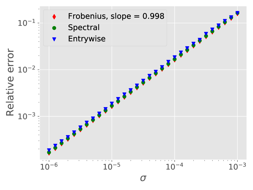
(a)

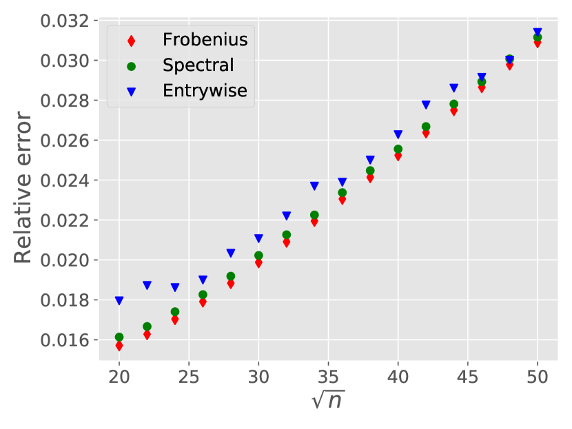
(b)

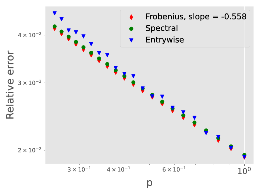
(c)

Figure 1: (a) Relative estimation error of $\bm{L}_{\mathrm{cvx}}$ vs. noise size $\sigma$ on a log-log scale, where we fix $n=500,r=5,p=0.5$; (b) Relative estimation error of $\bm{L}_{\mathrm{cvx}}$ vs. problem size $\sqrt{n}$, where we fix $r=5,\sigma=10^{-4},p=0.5$; (c) Relative estimation error of $\bm{L}_{\mathrm{cvx}}$ vs. observation probability $p$ on a log-log scale, where we fix $n=2000,r=5,\sigma=10^{-4}$. For all three plots, $\lambda=4/\sqrt{n}$ and each point represents the average of 20 independent trials.

3 Outline of the proof

In this section, we provide the key steps for proving our main result, i.e., Theorem 1. The proof follows the general strategy of bridging convex and nonconvex solutions, first appeared in the paper [CCF⁺20], with several important modifications to handle the non-smooth $\ell_{\mathrm{F}}$ norm (as opposed to the smooth squared $\ell_{\mathrm{F}}$ norm).

A central object in our analysis is the following nonconvex optimization problem

$$\min_{\text{$\bm{X}$,$\bm{Y}\in\mathbb{R}^{n\times r}$, $\theta>0$ }}\quad f(\bm{X},\bm{Y},\theta)\coloneqq\frac{1}{2}\left(\frac{\|\mathcal{P}_{\Omega}(\bm{X}\bm{Y}^{\top}-\bm{M})\|_{\mathrm{F}}^{2}}{\theta}+\theta\right)+\frac{\lambda}{2}\left(\|\bm{X}\|_{\mathrm{F}}^{2}+\|\bm{Y}\|_{\mathrm{F}}^{2}\right),$$ (5)

which is closely related to the original convex square-root MC formulation (3). To see this, first, for any rank-$r$ matrix $\bm{Z}$, one has

$$\|\bm{Z}\|_{*}=\inf_{\bm{X},\bm{Y}\in\mathbb{R}^{n\times r}:\bm{X}\bm{Y}^{\top}=\bm{Z}}\tfrac{1}{2}\left(\|\bm{X}\|_{\mathrm{F}}^{2}+\|\bm{Y}\|_{\mathrm{F}}^{2}\right).$$

Second and more importantly, we have that for any matrix $\bm{Z}=\bm{X}\bm{Y}^{\top}$,

$$\|\mathcal{P}_{\Omega}(\bm{Z}-\bm{M})\|_{\mathrm{F}}=\inf_{\theta>0}\quad\frac{1}{2}\left(\frac{\|\mathcal{P}_{\Omega}(\bm{X}\bm{Y}^{\top}-\bm{M})\|_{\mathrm{F}}^{2}}{\theta}+\theta\right).$$

It turns out that the (approximate) solution to the nonconvex optimization problem (5) serves as an extremely tight approximation to the square-root MC estimator, which facilitates the statistical analysis of the latter.

In sum, our proof involves two main steps:

1. We first show—via an explicit construction—that an approximate stationary point $\bm{L}_{\mathrm{ncvx}}$ of the nonconvex problem (5) exists and is also close to the groundtruth matrix $\bm{L}^{\star}$.

2. We then establish that such an approximate stationary point $\bm{L}_{\mathrm{ncvx}}$ is extremely close to the solution $\bm{L}_{\mathrm{cvx}}$ to the convex problem (3).

Combining the two key steps via triangle inequality finishes the proof.

Step 1: Nonconvex optimization.

The nonconvex optimization problem (5) has two groups of decision variables, i.e., $(\bm{X},\bm{Y})$ and $\theta$. Also note that given a fixed pair $(\bm{X},\bm{Y})$, the optimal choice of $\theta$ is simply given by $\theta=\|\mathcal{P}_{\Omega}(\bm{X}\bm{Y}^{\top}-\bm{M})\|_{\mathrm{F}}$. Therefore it is natural to consider an alternating minimization method to construct an approximate stationary point of the nonconvex program (5); see Algorithm 1. Given a current iterate $(\bm{X}_{t},\bm{Y}_{t},\theta_{t})$, the algorithm first runs one step of gradient descent on $(\bm{X},\bm{Y})$ while fixing $\theta_{t}$. It then updates $\theta_{t+1}=\|\mathcal{P}_{\Omega}(\bm{X}_{t+1}\bm{Y}_{t+1}^{\top}-\bm{M})\|_{\mathrm{F}}$ to be the optimal choice given the new iterate $(\bm{X}_{t+1},\bm{Y}_{t+1})$. In the end, Algorithm 1 returns the point $\bm{L}_{\mathrm{ncvx}}$ with the smallest gradient among the iterates as an approximate stationary point.

Algorithm 1 Gradient descent on the nonconvex formulation of square root matrix completion

Input: initialization$\bm{X}_{0}=\bm{X}^{\star},\bm{Y}_{0}=\bm{Y}^{\star},\theta_{0}=\|\mathcal{P}_{\Omega}(\bm{X}^{\star}\bm{Y}^{\star\top}-\bm{M})\|_{\mathrm{F}}$, step size $\eta\asymp\sigma/(\sqrt{p}\kappa^{3}\sigma_{\max})$, and total number of iterations $t_{0}=n^{18}$.

Gradient updates: for $t=0,1,\ldots,t_{0}-1$ do

$$\bm{X}_{t+1} =\bm{X}_{t}-\eta\nabla_{\bm{X}}f(\bm{X}_{t},\bm{Y}_{t},\theta_{t})=\bm{X}_{t}-\eta\left(\tfrac{1}{\theta_{t}}\mathcal{P}_{\Omega}(\bm{X}_{t}\bm{Y}_{t}^{\top}-\bm{M})\bm{Y}_{t}+\lambda\bm{X}_{t}\right);$$ (6a)

$$\bm{Y}_{t+1} =\bm{Y}_{t}-\eta\nabla_{\bm{Y}}f(\bm{X}_{t},\bm{Y}_{t},\theta_{t})=\bm{Y}_{t}-\eta\left(\tfrac{1}{\theta_{t}}\left[\mathcal{P}_{\Omega}(\bm{X}_{t}\bm{Y}_{t}^{\top}-\bm{M})\right]^{\top}\bm{X}_{t}+\lambda\bm{Y}_{t}\right);$$ (6b)

$$\theta_{t+1} =\|\mathcal{P}_{\Omega}(\bm{X}_{t+1}\bm{Y}_{t+1}^{\top}-\bm{M})\|_{\mathrm{F}}.$$ (6c)

Define

$$t^{\star}\coloneqq\arg\min_{0\leq t\leq t_{0}}\|\nabla_{\bm{X},\bm{Y}}f(\bm{X}_{t},\bm{Y}_{t},\theta_{t})\|_{\mathrm{F}},$$

where

$$\nabla_{\bm{X},\bm{Y}}f(\bm{X}_{t},\bm{Y}_{t},\theta_{t})=\begin{bmatrix}\frac{1}{\theta_{t}}\mathcal{P}_{\Omega}(\bm{X}_{t}\bm{Y}_{t}^{\top}-\bm{M})\bm{Y}_{t}+\lambda\bm{X}_{t}\\ \frac{1}{\theta_{t}}\left[\mathcal{P}_{\Omega}(\bm{X}_{t}\bm{Y}_{t}^{\top}-\bm{M})\right]^{\top}\bm{X}_{t}+\lambda\bm{Y}_{t}\end{bmatrix}.$$

Output: $\bm{L}_{\mathrm{ncvx}}\coloneqq\bm{X}_{t^{\star}}\bm{Y}_{t^{\star}}^{\top}$, $\bm{X}_{\mathrm{ncvx}}\coloneqq\bm{X}_{t^{\star}}$, and $\bm{Y}_{\mathrm{ncvx}}\coloneqq\bm{Y}_{t^{\star}}$.

The following lemma ensures that $\bm{L}_{\mathrm{ncvx}}$ is an approximate stationary point of the nonconvex problem and more importantly is close to the groundtruth matrix $\bm{L}^{\star}$. The proof is deferred to Section 3.1.

Lemma 1.

Instate the assumptions of Theorem 1. With probability at least $1-O(n^{-3})$, one has

$$\|\bm{L}_{\mathrm{ncvx}}-\bm{L}^{\star}\|_{\mathrm{F}} \leq 3\kappa C_{\mathrm{F}}\left(\frac{\sigma}{\sigma_{\min}}\sqrt{\frac{n}{p}}\right)\|\bm{L}^{\star}\|_{\mathrm{F}},$$ (7a)

$$\|\bm{L}_{\mathrm{ncvx}}-\bm{L}^{\star}\|_{\mathrm{\infty}} \leq 3\sqrt{\kappa^{3}\mu r}C_{\mathrm{\infty}}\left(\frac{\sigma}{\sigma_{\min}}\sqrt{\frac{n\log n}{p}}\right)\|\bm{L}^{\star}\|_{\mathrm{\infty}},$$ (7b)

$$\|\bm{L}_{\mathrm{ncvx}}-\bm{L}^{\star}\| \leq 3C_{\mathrm{op}}\left(\frac{\sigma}{\sigma_{\min}}\sqrt{\frac{n}{p}}\right)\|\bm{L}^{\star}\|,$$ (7c)

where $C_{\mathrm{F}},C_{\infty},C_{\mathsf{op}}$ are three universal positive constants.

Step 2: Bridging convex and nonconvex solutions.

It remains to show that $\bm{L}_{\mathrm{ncvx}}$ is extremely close to the convex solution $\bm{L}_{\mathrm{cvx}}$, which is provided in the following lemma.

Lemma 2.

Instate the assumptions of Theorem 1. With probability exceeding $1-O(n^{-3})$, one has

$$\left\|\bm{L}_{\mathrm{ncvx}}-\bm{L}_{\mathrm{cvx}}\right\|_{\mathrm{F}}\leq\frac{1}{n^{5}}\frac{\lambda\sigma}{\sigma_{\min}}\|\bm{L}^{\star}\|_{\mathrm{F}}.$$

See Section 3.2 for the proof of this lemma.

We remark in passing that the polynomial factor $n^{-5}$ in Lemma 2 is arbitrarily chosen, and the exponent $5$ can be replaced with any large constant. The essence is that the difference between $\bm{L}_{\mathrm{ncvx}}$ and $\bm{L}_{\mathrm{cvx}}$ is orderwise much smaller compared to the estimation error of $\bm{L}_{\mathrm{ncvx}}$ itself. Such proximity between $\bm{L}_{\mathrm{ncvx}}$ and $\bm{L}_{\mathrm{cvx}}$ is verified empirically in Figure 2.

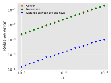
Figure 2: Relative Frobenius estimation error of convex and nonconvex solutions and their distance. The parameters are chosen as: $n=200,r=5,p=0.5$ while $\sigma$ varies from $10^{-5}$ to $10^{-3}$.

Now we are ready to combine the previous two steps and finish the proof of Theorem 1.

Proof of Theorem 1.

Combine Lemmas 1-2 with the triangle inequality to arrive at

$$\left\|\bm{L}_{\mathrm{cvx}}-\bm{L}^{\star}\right\|_{\mathrm{F}} \leq\left\|\bm{L}_{\mathrm{ncvx}}-\bm{L}_{\mathrm{cvx}}\right\|_{\mathrm{F}}+\left\|\bm{L}_{\mathrm{ncvx}}-\bm{L}^{\star}\right\|_{\mathrm{F}}$$

$$\leq\left[\frac{1}{n^{5}}\frac{\lambda\sigma}{\sigma_{\min}}+3\kappa C_{\mathrm{F}}\left(\frac{\sigma}{\sigma_{\min}}\sqrt{\frac{n}{p}}\right)\right]\|\bm{L}^{\star}\|_{\mathrm{F}}$$

$$\leq 4\kappa C_{\mathrm{F}}\left(\frac{\sigma}{\sigma_{\min}}\sqrt{\frac{n}{p}}\right)\|\bm{L}^{\star}\|_{\mathrm{F}},$$

where the last relation uses the facts that $\lambda\asymp 1/\sqrt{n}$ and that $p\gtrsim 1/\sqrt{n}$. Redefine $4C_{\mathrm{F}}$ to be $C_{\mathrm{F}}$ to complete the proof of the bound (4a). The other two bounds on the operator norm and the $\ell_{\infty}$ norm follow from similar arguments. We omit here for brevity.

3.1 Proof of Lemma 1

Since Algorithm 1 operates in the space of low-rank factors, we start with establishing guarantees for the stacked low-rank factor $\bm{F}_{t}\coloneqq\begin{bmatrix}\bm{X}_{t}\\ \bm{Y}_{t}\end{bmatrix}\in\mathbb{R}^{2n\times r}$, and then translate the guarantees to the matrix space $\bm{L}_{t}=\bm{X}_{t}\bm{Y}_{t}^{\top}$. Special care is needed as the decomposition $\bm{L}=\bm{X}\bm{Y}^{\top}$ is not unique in $(\bm{X},\bm{Y})$, and hence we need to account for the rotational ambiguity in $(\bm{X},\bm{Y})$. To this end, for each $t\geq 0$, we define the optimal rotation matrix to be

$$\bm{H}_{t}\coloneqq\mathrm{argmin}_{\bm{R}\in\mathcal{O}^{r\times r}}\quad\|\bm{X}_{t}\bm{R}-\bm{X}^{\star}\|_{\mathrm{F}}^{2}+\|\bm{Y}_{t}\bm{R}-\bm{Y}^{\star}\|_{\mathrm{F}}^{2}.$$ (8)

Introducing leave-one-out sequences.

In order to control the $\ell_{2,\infty}$ error of $\bm{F}_{t}$ (and hence $\ell_{\infty}$ error of $\bm{L}_{t}$), we construct $2n$ leave-one-out auxiliary sequences $\{\bm{F}_{t}^{(l)}\}_{1\leq l\leq 2n,t\geq 0}$. The hope is that $\{\bm{F}_{t}^{(l)}\}_{1\leq l\leq 2n,t\geq 0}$ serves as a good approximation to the original sequence $\{\bm{F}_{t}\}_{t\geq 0}$, while at the same time is more amenable to statistical analysis.

To formally construct such leave-one-out sequences, we first define $2n$ auxiliary loss functions. For each $1\leq l\leq n$, define

$$f^{(l)}(\bm{X},\bm{Y},\theta)=\frac{1}{2}\left(\frac{\|\mathcal{P}_{\Omega_{-l,\cdot}}(\bm{L}-\bm{M})\|_{\mathrm{F}}^{2}+p\|\mathcal{P}_{l,\cdot}(\bm{L}-\bm{M})\|_{\mathrm{F}}^{2}}{\theta}+\theta\right)+\frac{\lambda}{2}\left(\|\bm{X}\|_{\mathrm{F}}^{2}+\|\bm{Y}\|_{\mathrm{F}}^{2}\right)$$

where

$$\left[\mathcal{P}_{\Omega_{-l,\cdot}}(\bm{B})\right]_{ij}=\begin{cases}B_{ij},&\text{if }(i,j)\in\Omega\text{ and }i\neq l\\ 0,&\text{otherwise}\end{cases},\quad\text{and}\quad\left[\mathcal{P}_{l,\cdot}(\bm{B})\right]_{ij}=\begin{cases}B_{ij},&\text{if }i=l\\ 0,&\text{otherwise}\end{cases}.$$

Similarly, for each $n+1\leq l\leq 2n$, we define

$$f^{(l)}(\bm{X},\bm{Y},\theta)=\frac{1}{2}\left(\frac{\|\mathcal{P}_{\Omega_{\cdot,-(l-n)}}(\bm{L}-\bm{M})\|_{\mathrm{F}}^{2}+p\|\mathcal{P}_{l,\cdot}(\bm{L}-\bm{M})\|_{\mathrm{F}}^{2}}{\theta}+\theta\right)+\frac{\lambda}{2}\left(\|\bm{X}\|_{\mathrm{F}}^{2}+\|\bm{Y}\|_{\mathrm{F}}^{2}\right)$$

where

$$\left[\mathcal{P}_{\Omega_{\cdot,-(l-n)}}(\bm{B})\right]_{ij}=\begin{cases}B_{ij},&\text{if }(i,j)\in\Omega\text{ and }j\neq l-n\\ 0,&\text{otherwise}\end{cases}\quad\text{and}\quad\left[\mathcal{P}_{l,\cdot}(\bm{B})\right]_{ij}=\begin{cases}B_{ij},&\text{if }j=l-n\\ 0,&\text{otherwise}\end{cases}.$$

With these notations in place, Algorithm 2 details the way we construct the leave-one-out sequences.

Algorithm 2 Gradient descent generating the leave-one-out sequences

Initialization: $\bm{X}_{0}^{(l)}=\bm{X}^{\star},\bm{Y}_{0}^{(l)}=\bm{Y}^{\star},\theta_{0}^{(l)}=\|\mathcal{P}_{\Omega}(\bm{X}^{\star}\bm{Y}^{\star\top}-\bm{M})\|_{\mathrm{F}}$, step size $\eta\asymp\sigma/(\sqrt{p}\kappa^{3}\sigma_{\max})$, and total number of iterations $t_{0}=n^{18}$.

Gradient updates: for $t=0,1,\cdots,t_{0}-1$ do

$$\bm{X}_{t+1}^{(l)} =\bm{X}_{t}^{(l)}-\eta\nabla_{\bm{X}}f^{(l)}(\bm{X}_{t}^{(l)},\bm{Y}_{t}^{(l)},\theta_{t});$$ (9a)

$$\bm{Y}_{t+1}^{(l)} =\bm{Y}_{t}^{(l)}-\eta\nabla_{\bm{Y}}f^{(l)}(\bm{X}_{t}^{(l)},\bm{Y}_{t}^{(l)},\theta_{t});$$ (9b)

$$\theta_{t+1} =\left\|\mathcal{P}_{\Omega}\left(\bm{X}_{t+1}\bm{Y}_{t+1}^{\top}-\bm{M}\right)\right\|_{\mathrm{F}}.$$ (9c)

Similar constructions have been deployed in the papers [CCF⁺20] and [CFMY21]. However, it is worth pointing out that the sequence $\{\theta_{t}\}$ is produced according to the original sequence, instead of the leave-one-out sequence. This change is tailored to the analysis of the square-root MC estimator as it aligns better with the original loss function $f$, while allowing us to reuse several keys results in the paper [CCF⁺20].

Properties of the iterates.

As planned, we aim to show that the leave-one-out iterates $\{\bm{F}_{t}^{(l)}\}_{1\leq l\leq 2n,t\geq 0}$ stay extremely close to the original iterates $\{\bm{F}_{t}\}_{t\geq 0}$, and that $\{\bm{F}_{t}\}_{t\geq 0}$ is close to the groundtruth factor $\bm{F}^{\star}$. Such properties are collected in the following lemma.

Lemma 3.

With probability at least $1-O(n^{-3})$, the following statements hold for all iterations $0\leq t\leq t_{0}$:

$$\|\bm{F}_{t}\bm{H}_{t}-\bm{F}^{\star}\|_{\mathrm{F}} \leq C_{\mathrm{F}}\frac{\sigma}{\sigma_{\min}}\sqrt{\frac{n}{p}}\|\bm{X}^{\star}\|_{\mathrm{F}},$$ (10a)

$$\|\bm{F}_{t}\bm{H}_{t}-\bm{F}^{\star}\| \leq C_{\mathrm{op}}\frac{\sigma}{\sigma_{\min}}\sqrt{\frac{n}{p}}\|\bm{X}^{\star}\|,$$ (10b)

$$\max_{1\leq l\leq 2n}\|\bm{F}_{t}\bm{H}_{t}-\bm{F}_{t}^{(l)}\bm{R}_{t}^{(l)}\|_{\mathrm{F}} \leq C_{\mathrm{3}}\frac{\sigma}{\sigma_{\min}}\sqrt{\frac{n\log n}{p}}\|\bm{F}^{\star}\|_{2,\infty},$$ (10c)

$$\max_{1\leq l\leq 2n}\|(\bm{F}_{t}^{(l)}\bm{H}_{t}^{(l)}-\bm{F}^{\star})_{l,\cdot}\|_{\mathrm{F}} \leq C_{\mathrm{4}}\kappa\frac{\sigma}{\sigma_{\min}}\sqrt{\frac{n\log n}{p}}\|\bm{F}^{\star}\|_{2,\infty},$$ (10d)

$$\|\bm{F}_{t}\bm{H}_{t}-\bm{F}^{\star}\|_{2,\infty} \leq C_{\mathrm{\infty}}\kappa\frac{\sigma}{\sigma_{\min}}\sqrt{\frac{n\log n}{p}}\|\bm{F}^{\star}\|_{2,\infty},$$ (10e)

for some positive constants $C_{\mathrm{F}},C_{\mathrm{op}},C_{3},C_{4},C_{\infty}$. Here $\bm{H}_{t}^{(l)}$ and $\bm{R}_{t}^{(l)}$ are defined as

$$\bm{H}_{t}^{(l)} \coloneqq\mathrm{argmin}_{\bm{R}\in\mathcal{O}^{r\times r}}\|\bm{F}_{t}^{(l)}\bm{R}-\bm{F}^{\star}\|_{\mathrm{F}}$$

$$\bm{R}_{t}^{(l)} \coloneqq\mathrm{argmin}_{\bm{R}\in\mathcal{O}^{r\times r}}\|\bm{F}_{t}^{(l)}\bm{R}-\bm{F}_{t}\bm{H}_{t}\|_{\mathrm{F}}.$$

Furthermore the output $(\bm{X}_{t^{\star}},\bm{Y}_{t^{\star}})$ has small gradient:

$$\|\nabla_{\bm{X},\bm{Y}}f(\bm{X}_{t^{\star}},\bm{Y}_{t^{\star}},\theta_{t^{\star}})\|_{\mathrm{F}}\leq C_{\mathrm{grad}}\frac{1}{n^{8}}\sqrt{\frac{\sigma_{\max}}{p}}.$$ (11)

See Section A for the proof of this lemma.

Now we are ready to prove Lemma 1 based on the results presented in Lemma 3.

Proof of Lemma 1.

By the triangle inequality, one has

$$\|\bm{X}_{t^{\star}}\bm{Y}_{t^{\star}}^{\top}-\bm{L}^{\star}\| \leq\|\bm{X}_{t^{\star}}\bm{Y}_{t^{\star}}^{\top}-\bm{X}_{t^{\star}}\bm{Y}^{\star\top}\|+\|\bm{X}_{t^{\star}}\bm{Y}^{\star\top}-\bm{L}^{\star}\|$$

$$\leq\|\bm{Y}_{t^{\star}}-\bm{Y}^{\star}\|\|\bm{X}_{t^{\star}}\|+\|\bm{X}_{t^{\star}}-\bm{X}^{\star}\|\|\bm{Y}^{\star}\|.$$

Use relation (10b) to obtain

$$\|\bm{X}_{t^{\star}}\bm{Y}_{t^{\star}}^{\top}-\bm{L}^{\star}\| \leq 3C_{\mathrm{op}}\frac{\sigma}{\sigma_{\min}}\sqrt{\frac{n}{p}}\|\bm{X}^{\star}\|\|\bm{X}^{\star}\|=3C_{\mathrm{op}}\frac{\sigma}{\sigma_{\min}}\sqrt{\frac{n}{p}}\|\bm{L}^{\star}\|.$$

The first inequality uses $\|\bm{X}_{t^{\star}}\|\leq 2\|\bm{X}^{\star}\|$, which is a direct consequence of (10b) and the last line uses $\|\bm{L}^{\star}\|=\sigma_{\max}=\|\bm{X}^{\star}\|^{2}$. Similarly we have

$$\|\bm{X}_{t^{\star}}\bm{Y}_{t^{\star}}^{\top}-\bm{L}^{\star}\|_{\mathrm{F}}\leq 3C_{\mathrm{\mathrm{F}}}\frac{\sigma}{\sigma_{\min}}\sqrt{\frac{n}{p}}\|\bm{X}^{\star}\|_{\mathrm{F}}\|\bm{X}^{\star}\|\overset{(\text{i})}{\leq}3\kappa C_{\mathrm{op}}\frac{\sigma}{\sigma_{\min}}\sqrt{\frac{n}{p}}\|\bm{L}^{\star}\|_{\mathrm{F}}$$

and

$$\|\bm{X}_{t^{\star}}\bm{Y}_{t^{\star}}^{\top}-\bm{L}^{\star}\|_{\infty}\leq 3C_{\mathrm{\infty}}\frac{\sigma}{\sigma_{\min}}\sqrt{\frac{n\log n}{p}}\|\bm{F}^{\star}\|_{2,\infty}\|\bm{F}^{\star}\|_{2,\infty}\overset{(\text{ii})}{\leq}3\sqrt{\kappa^{3}\mu r}C_{\infty}\frac{\sigma}{\sigma_{\min}}\sqrt{\frac{n\log n}{p}}\|\bm{L}^{\star}\|_{\infty}.$$

Here step (i) uses the fact$\|\bm{X}^{\star}\|_{\mathrm{F}}\|\bm{X}^{\star}\|\leq\kappa\|\bm{L}^{\star}\|_{\mathrm{F}}$, whereas in step (ii) we use

$$\|\bm{F}^{\star}\|_{2,\infty}\|\bm{F}^{\star}\|_{2,\infty}\leq\sqrt{\kappa^{3}\mu r}\|\bm{L}^{\star}\|_{\infty}.$$

3.2 Proof of Lemma 2

Before embarking on the main proof, we state a few useful properties of the noise matrix $\bm{E}$ and the nonconvex solution $\bm{L}_{\mathrm{ncvx}}$. These properties allow us to establish the proximity between the approximate stationary point $\bm{L}_{\mathrm{ncvx}}$ and the convex solution $\bm{L}_{\mathrm{cvx}}$.

The first property is concerned with the size of the regularization parameter, which appeared as Lemma 3 in the paper [CCF⁺20].

Lemma 4.

Suppose that $n^{2}p\geq Cn\log^{2}n$ for some sufficiently large constant $C>0$. Take $\lambda=C_{\lambda}/\sqrt{n}$ for some absolute constant $C_{\lambda}$. Then with probability at least $1-O(n^{-10})$, one has

$$\|\mathcal{P}_{\Omega}(\bm{E})\|\leq\frac{\lambda}{16}np^{1/2}\sigma.$$ (12)

The next property is on the injectivity of $\mathcal{P}_{\Omega}$ in the tangent space $T$ at $\bm{L}_{\mathrm{ncvx}}$. More precisely, letting $\bm{U\Sigma V}^{\top}$ be the SVD of $\bm{L}_{\mathrm{ncvx}}$, we define the tangent space $T$ at $\bm{L}_{\mathrm{ncvx}}$ as

$$T=\left\{\bm{U}\bm{A}^{\top}+\bm{B}\bm{V}^{\top}\mid\bm{A},\bm{B}\in\mathbb{R}^{n\times r}\right\}.$$

Lemma 5.

Instate the assumptions of Theorem 1. With probability exceeding $1-O(n^{-3})$, for all $\bm{H}\in T$

$$p^{-1/2}\|\mathcal{P}_{\Omega}(\bm{H})\|_{\mathrm{F}}\geq C_{\mathrm{inj}}\|\bm{H}\|_{\mathrm{F}},\qquad\text{where}\quad C_{\mathrm{inj}}=(32\kappa)^{-1/2}.$$ (13)

Proof.

This is an easy consequence of Lemma 4 in the paper [CCF⁺20] and the relation (10e). ∎

Last but not least, the lemma collects several interesting properties of the nonconvex solution $\bm{L}_{\mathrm{ncvx}}$, as well as its low-rank factors $\bm{X}_{\mathrm{ncvx}},\bm{Y}_{\mathrm{ncvx}}$.

Lemma 6.

The approximate stationary point $\bm{L}_{\mathrm{ncvx}}$ satisfies

$$\sqrt{\sigma_{\min}/2}\leq\sigma_{\min}(\bm{X}_{\mathrm{ncvx}})\leq\sigma_{\max}(\bm{X}_{\mathrm{ncvx}}) \leq\sqrt{2\sigma_{\max}};$$ (14a)

$$\sqrt{\sigma_{\min}/2}\leq\sigma_{\min}(\bm{Y}_{\mathrm{ncvx}})\leq\sigma_{\max}(\bm{Y}_{\mathrm{ncvx}}) \leq\sqrt{2\sigma_{\max}};$$ (14b)

$$\frac{1}{2}np^{1/2}\sigma\leq\|\mathcal{P}_{\Omega}(\bm{L}_{\mathrm{ncvx}}-\bm{M})\|_{\mathrm{F}} \leq 2np^{1/2}\sigma;$$ (14c)

$$\|\mathcal{P}_{\Omega}(\bm{X}\bm{Y}^{\top}-\bm{L}^{\star})-p(\bm{X}\bm{Y}^{\top}-\bm{L}^{\star})\| \leq\frac{\lambda}{16}np^{1/2}\sigma.$$ (14d)

See Section A.4 for the proof of this lemma.

For notational simplicity, we define

$$g(\bm{X},\bm{Y})\coloneqq f(\bm{X},\bm{Y},\|\mathcal{P}_{\Omega}(\bm{X}\bm{Y}^{\top}-\bm{M})\|_{\mathrm{F}})=\|\mathcal{P}_{\Omega}(\bm{X}\bm{Y}^{\top}-\bm{M})\|_{\mathrm{F}}+\frac{\lambda}{2}\left(\|\bm{X}\|_{\mathrm{F}}^{2}+\|\bm{Y}\|_{\mathrm{F}}^{2}\right).$$

In other words, $g(\bm{X},\bm{Y})$ is the minimal value of $f(\bm{X},\bm{Y},\theta)$ when $(\bm{X},\bm{Y})$ is fixed.

Now we are ready to present the key lemma of this section, which relates the difference between $\bm{L}_{\mathrm{ncvx}}$ and $\bm{L}_{\mathrm{cvx}}$ to the size of the gradient $\nabla g(\bm{X}_{\mathrm{ncvx}},\bm{Y}_{\mathrm{ncvx}})$. The proof is deferred to Section B.

Lemma 7.

Suppose that $(\bm{X}_{\mathrm{ncvx}},\bm{Y}_{\mathrm{ncvx}})$ has small gradient in the sense that

$$\left\|\nabla g(\bm{X}_{\mathrm{ncvx}},\bm{Y}_{\mathrm{ncvx}})\right\|_{\mathrm{F}}\leq\frac{\sqrt{\sigma_{\min}}}{280\kappa}\max\left\{C_{\mathrm{inj}}\sqrt{p},\frac{1}{2}\lambda^{2}n\sigma\right\}.$$ (15)

Then on the event that Lemmas 4-6 hold, any minimizer $\bm{L}_{\mathrm{cvx}}$ of the convex program (3) satisfies

$$\left\|\bm{L}_{\mathrm{ncvx}}-\bm{L}_{\mathrm{cvx}}\right\|_{\mathrm{F}}\leq\frac{\lambda\kappa^{2}}{\sqrt{p\sigma_{\min}}}n\sigma\|\nabla g(\bm{X}_{\mathrm{ncvx}},\bm{Y}_{\mathrm{ncvx}})\|_{\mathrm{F}}.$$

Remark 1.

Observe that if $\|\nabla g(\bm{X}_{\mathrm{ncvx}},\bm{Y}_{\mathrm{ncvx}})\|_{\mathrm{F}}=0$, i.e., if $\bm{L}_{\mathrm{ncvx}}$ is an exact stationary point of the nonconvex square-root MC problem, $\bm{L}_{\mathrm{ncvx}}$ is also a solution to the convex problem (3).

With the help of Lemma 7, we can prove Lemma 2 now.

Proof of Lemma 2.

First, Lemma 3 tells us that the nonconvex solution $(\bm{X}_{t^{\star}},\bm{Y}_{t^{\star}})$ satisfies the bound (15) on the size of the gradient. This together with Lemmas 4 to 6 allows us to invoke Lemma 7 to obtain

$$\left\|\bm{L}_{\mathrm{ncvx}}-\bm{L}_{\mathrm{cvx}}\right\|_{\mathrm{F}} \lesssim\frac{\lambda\kappa^{2}}{\sqrt{p\sigma_{\min}}}n\sigma\|\nabla g(\bm{X}_{\mathrm{ncvx}},\bm{Y}_{\mathrm{ncvx}})\|_{\mathrm{F}}\lesssim\frac{1}{n^{5}}\frac{\lambda\sigma}{\sigma_{\min}}\|\bm{L}^{\star}\|_{\mathrm{F}},$$

where the last inequality uses the gradient upper bound (15), $\|\bm{L}^{\star}\|_{\mathrm{F}}\geq\|\bm{L}^{\star}\|\geq\sigma_{\max}=\kappa\sigma_{\min}$, and the fact that the sample size assumption $n^{2}p\geq C_{\mathrm{sample}}\kappa^{4}\mu^{2}r^{2}n\log^{3}n$ implies $np\gtrsim 1$ and $\kappa\lesssim n$.

4 Simulation

In this section, we further illustrate the performance of the tuning-free square root matrix completion through two sets of comparative simulation studies. First we compare the performance of square-root MC to the non-sqaure-root estimator (2) with oracle and cross-validated parameters. This allows us to examine whether we sacrifice a significant amount of performance in achieving the tuning-free property. Second, we do the same comparison on approximately low rank matrices. This helps us understand how robust the estimator is against misspecified low-rank assumption.

Comparing square-root MC with standard approach (2).

For the non-square-root approach (2), as the sampling probability $p$ and noise level $\sigma$ is unknown, the regularization parameter needs to be carefully chosen. Here we compare square-root MC with (2) using oracle and $k$-fold cross-validated regularization parameters, namely

$$\lambda_{\mathrm{oracle}}\coloneqq\arg\min_{\lambda}\quad\left\|\bm{L}^{\star}-\hat{\bm{L}}_{\lambda,\Omega}\right\|_{\mathrm{F}},$$

$$\lambda_{\mathrm{CV}}\coloneqq\arg\min_{\lambda}\quad\sum_{i=1}^{k}\left\|\mathcal{P}_{\Omega_{i}}\left(\bm{L}-\hat{\bm{L}}_{\lambda,\Omega_{-i}}\right)\right\|_{\mathrm{F}}^{2},$$

where

$$\hat{\bm{L}}_{\lambda,\Omega}\coloneqq\arg\min_{\bm{L}\in\mathbb{R}^{n\times n}}\quad\sum_{(i,j)\in\Omega}(L_{ij}-M_{ij})^{2}+\lambda\|\bm{L}\|_{*}$$

with $\Omega_{i}$ being the $i$-th fold of the sampled entries and $\Omega_{-i}\coloneqq\Omega\setminus\Omega_{i}$ . Due to computational limit, our experiment uses estimates $\hat{\lambda}_{\mathrm{oracle}},\hat{\lambda}_{\mathrm{CV}}$ obtained by taking minimum over a discrete set of parameters that is close to the true $\lambda_{\mathrm{oracle}}$. In practice $\lambda_{\mathrm{oracle}}$ is inaccessible as we do not know $\bm{L}^{\star}$. Meanwhile $\lambda_{\mathrm{CV}}$ takes $k\cdot n_{\lambda}$ runs of an algorithm for (2) to obtain, where $n_{\lambda}$ is the number of $\lambda$’s one tries in cross-validation. This can be computationally prohibitive when the matrices of interest have different sampling rate $p$ and noise level $\sigma$, in which case cross-validation is needed for each matrix in order to get a reasonable $\lambda$. In comparison, the tuning-free property of square-root MC makes the regularization parameter much easier to obtain.

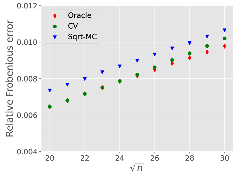
(a)

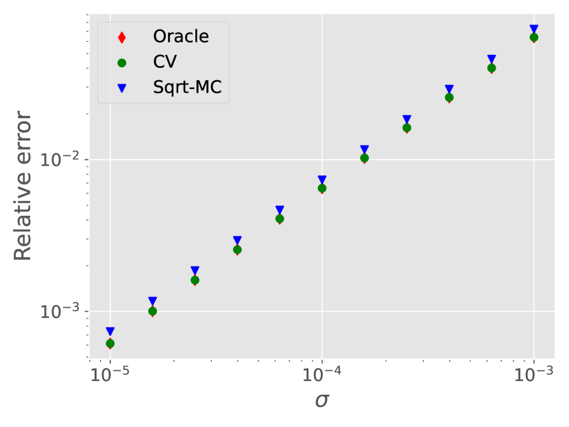
(b)

Figure 3: (a) Relative Frobenius estimation error of square-root MC and solution of (2) with oracle and cross-validated $\lambda$ vs. problem size $\sqrt{n}$. The parameters are fixed as $\sigma=10^{-4},r=5,p=0.5$. (b) Relative Frobenius estimation error of square-root MC and solution of (2) with oracle and cross-validated $\lambda$ vs. noise size $\sigma$ on a log-log scale. The parameters are fixed as $n=400,r=5,p=0.5$. In both settings, $k=10$ for the number of folds in cross validation and each point represents the average of 10 independent trials.

In each run of the experiment, we first generate an $n\times n$ matrix $\bm{M}$ as in (1) and calculate its estimator using square-root MC with fixed regularization parameter $\lambda=2/\sqrt{n}$ and (2) with $\hat{\lambda}_{\mathrm{oracle}}$ and 10-fold cross-validated $\hat{\lambda}_{\mathrm{CV}}$. Figure 3 shows the relative Frobenius errors of the different methods across varying matrix size $n$ and varying noise level $\sigma$. In both settings, we can see while square-root MC has very close estimation error to that of (2). Moreover their linear trends over problem size $\sqrt{n}$ and noise size $\sigma$ are similar, as we expect from their identical error rate. This shows that by using square-root MC, we achieve the tuning-free property with a minor sacrifice in the rate of estimation performance.

Performance with approximately low-rank matrices.

Another point of interest is whether square-root MC is robust to misspecification of the low-rank assumption. Here we conduct the experiment with approximately rank-$r$ matrices $\bm{L}^{\star}$ that singular values $\sigma_{1},\cdots,\sigma_{r}=1$ and $\sigma_{l}\propto(n-l)^{-2}$ such that $\sum_{l=r+1}^{n}\sigma_{l}\eqqcolon\gamma$. This parameter $\gamma$ can be viewed as a measurement of deviation from the set rank-$r$ matrices, as

$$\gamma=\min_{\bm{L}:\mathrm{rank}(\bm{L})=r}\|\bm{L}^{\star}-\bm{L}\|_{\ast}.$$

We then perform the same experiments as above, i.e., comparing square-root MC to (2) with oracle and cross-validated $\lambda$. Figure 4 shows their respective estimation error vs $\gamma$. We can see that the estimation error for all three methods increases when $\gamma$ increases and the increments are small and comparable across the three methods. This shows that square-root MC and (2) to are somewhat robust to the violation of low rank assumption.

In addition, we showcase an interesting discovery which compares the robustness of convex and nonconvex version of square-root MC to approximate low-rankness. We generate the ground-truth matrices that is approximately low rank and calculate square-root MC and the nonconvex solution of (5) assuming the rank is $r$. Figure 5 shows that the performance of square-root MC for approximately low rank matrices is close to the case with exact low-rankness ($\gamma=0$), while the nonconvex method suffers a much greater loss in estimation accuracy. The difference between convex and nonconvex method is close to 0 when $\gamma=0$ and increases drastically as $\gamma$ increases. To some extent, this is expected as the convex method does not require the input of rank information.

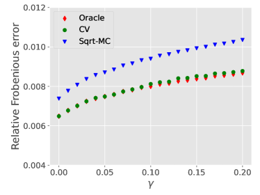
Figure 4: Relative Frobenius estimation error of square-root MC and solution of (2) with oracle and cross-validated $\lambda$ vs. $\gamma$ for approximately low rank matrices. The parameters are chosen as: $n=400,r=5,p=0.5,\sigma=10^{-4},\lambda=2/\sqrt{n}$ while $\gamma$ varies from $0$ to $0.2$. Each point represents the average of 10 independent trials.

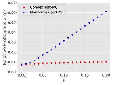
Figure 5: Relative Frobenius estimation error of square-root MC and (5) for approximately low rank matrices. The parameters are chosen as: $n=400,r=5,p=0.5,\sigma=10^{-4},\lambda=2/\sqrt{n}$ while $\gamma$ varies from $0$ to $0.2$. Each point represents the average of 10 independent trials.

5 Prior art

Matrix completion.

Convex relaxation has been extensively studied for the matrix completion problem both in the noiseless setting [CR09, CT10, Gro11, Rec11, Che15], and the noisy case [CP10, NW12, KLT11, Klo14, CCF⁺20]. In the noiseless setting, convex relaxation achieves exact recovery as soon as the number of observed entries $n^{2}p$ exceeds $nr\log n\log r$ [DC20]—roughly the degrees of freedom of a rank-$r$ matrix, which is information-theoretically optimal. When it comes to the noisy setting, Candès and Plan [CP10] focuses on arbitrary noise (e.g., noise could be deterministic and adversarial), and proves that convex relaxation is stable w.r.t. the noise size. The theoretical guarantees for convex relaxation are strengthened by Chen et al. [CCF⁺20] in the stochastic noise case, which is the same setting we study in the current paper. Such a discrepancy between stochastic and deterministic noise for convex relaxation is also documented in [KS21].

Pioneered by the work [KMO10, KMO09], nonconvex optimization has gained a lot of attentions during the past decade for solving matrix completion owing to its computational efficiency. Efficient computational and statistical guarantees have been provided for manifold optimization [KMO10, KMO09], gradient descent [MWCC18, CLL20], projected gradient descent [CW15, ZL16], alternating minimization [JNS13, Har14], scaled gradient descent [TMC21], singular value projection [DC20], etc. See the recent surveys [DR16, CLC19] for more related work on matrix completion.

Tuning-free methods.

A variety of tuning-free methods have been proposed to tackle high-dimensional linear regression. The seminal work [BCW11] proposes the square-root Lasso estimator which does not rely on knowing the size of the noise and is also statistically optimal. [SZ12] proposes an equivalent method named scaled sparse linear regression, which originates from the concomitant scale estimation [Hub11, Owe07]. [LM15] proposes TREX, a method similar to square-root Lasso and is completely parameter-free. [WPB⁺20] borrows ideas from non-parametric statistics and proposes Rank Lasso, whose optimal choice of tuning parameter can be simulated easily in the case with unknown variance of the noise. See [WW19] for a survey on the selection of tuning-parameters for high-dimensional regression and [GHV12] for a survey on regression with unknown variance of noise.

Bridging convex and nonconvex optimization.

The connections between convex and nonconvex optimization has been extensively used in a recent line of work. Chen et al. [CCF⁺20] uses this to prove the optimality of the vanilla least-squares estimator for noisy matrix completion; Later, the papers [CFMY21, CFWY21, WF22] extend the technique to the robust PCA problem, the blind deconvolution problem, and matrix completion with heavy-tailed noise.

Leave-one-out analysis.

Leave-one-out analysis is powerful in decoupling statistical dependence and obtain element-wise performance guarantees. It has been successfully applied to high-dimensional regression [EKBB⁺13, EK18], phase synchronization [ZB18], ranking [CFMW19, CGZ22], matrix completion [MWCC18, CLL20, AFWZ20], reinforcement learning [PW20], high-dimensional inference [CFMY19, YCF21] to name a few. Interested readers are referred to a recent overview [CCF⁺21] for detailed discussions.

6 Discussions

Focusing on the noisy matrix completion problem, this paper shows that a tuning-free estimator—square-root MC achieves optimal statistical performance. This opens up several interesting avenues for future research. Below, we list a few of them.

• Extensions to robust PCA. While our work focuses on matrix completion, a natural extension is to further consider partial observations with outliers, i.e., robust PCA. As mentioned, Zhang et al. [ZYW21] has studied this problem (with full observation) and provides an error guarantee of order $O(\sigma n^{2})$, which is sub-optimal in its dependency on the problem dimension. By contrast, a vanilla least-squares estimator with noise-size-dependent choice of $\lambda$ has been shown to be optimal [CFMY21]. It remains to be seen whether one can devise an optimal tuning-free method for robust PCA with noise and missing data.

• Inference for square-root MC estimator. The current paper discusses solely the estimation performance of the tuning-free estimator. As statistical inference for matrix completion is equally important, one wishes to develop inferential procedures around the square-root MC estimator as that has been done in the paper [CFMY19] for the vanilla least-squares estimator.

• Robustness to non-uniform design. In high-dimensional linear regression, optimal tuning-free methods have been developed to be adaptive to both the unknown noise size and the design matrix. In the matrix completion setting, the design is governed by the sampling pattern, which is assumed to be uniform in the current paper. It is of great interest to develop robust and tuning-free approaches for noisy matrix completion with non-uniform sampling that improve over the max-norm constrained estimator in [Klo14].

Appendix A Proof of Lemma 3

We prove Lemma 3 via induction. Since all the algorithms start from the groundtruth, it is trivial to see that the hypotheses (10) hold for $t=0$. We also record two important properties of the iterates at $t=0$, namely,

$$\frac{1}{2}np^{1/2}\sigma\leq\theta_{t}\leq 2np^{1/2}\sigma$$ (16)

and

$$\|\bm{X}_{t}^{\top}\bm{X}_{t}-\bm{Y}_{t}^{\top}\bm{Y}_{t}\|_{\mathrm{F}}\leq C_{\mathrm{B}}\kappa\eta\frac{\sigma}{\sigma_{\min}}\sqrt{\frac{n}{p}}\sqrt{r}\sigma_{\max}^{2},$$ (17)

where $C_{\mathrm{B}}>0$ is a universal constant. Note that at $t=0$, we have $\theta_{0}=\|\mathcal{P}_{\Omega}(\bm{E})\|_{\mathrm{F}}$, which concentrates sharply around $np^{1/2}\sigma$ under the noise assumption and uniform sampling.

Now suppose the hypotheses (10), (16), and (17) hold for the $t$-the iterates. We aim to show that the same set of hypotheses continue to hold for the $(t+1)$-th iterates. Sections A.1 and A.2 are devoted to this induction step. In addition, we prove the last claim (11) in Section A.3. In Section A.4 we prove Lemma 6 which is a consequence of (10) and (16).

A.1 Induction on hypotheses (10) and (17)

Define

$$\tilde{\lambda}_{t}\coloneqq\lambda\theta_{t},\qquad\text{and}\qquad\tilde{\eta}_{t}\coloneqq\eta/\theta_{t}.$$

We make a key observation that the $t$-th iterations of Algorithm 1 and 2 are exactly the same as the $t$-th iterations of Algorithm 1 (vanilla gradient descent) and 2 (construction of the leave-one-out sequence) in the paper [CCF⁺20] with the parameters $\tilde{\lambda}_{t}$ and $\tilde{\eta}_{t}$. Moreover, given the induction hypothesis (16) one has $\frac{1}{2}n\sqrt{p}\sigma\leq\theta_{t-1}\leq 2n\sqrt{p}\sigma$. Combine this with our choice of $\lambda=C_{\lambda}n^{-1/2}$ to see that

$$\tilde{\lambda}_{t}\asymp\sigma\sqrt{np},\qquad\text{and$\qquad$$\tilde{\eta}_{t}\asymp 1/(np\kappa^{3}\sigma_{\max})$}.$$

which are consistent with the choice of $\lambda$ and $\eta$ in [CCF⁺20]. These allow us to invoke Lemmas 10-15 in [CCF⁺20] to prove that claims (10) and (17) hold for the $(t+1)$-th iterates.

A.2 Induction on hypotheses (16)

In this section, we aim to show that the claim (16) holds for the $(t+1)$-th iterates.

Observe that

$$\mathcal{P}_{\Omega}\left(\bm{X}_{t+1}\bm{Y}_{t+1}^{\top}-\bm{M}\right)=\mathcal{P}_{\Omega}\left(\bm{X}_{t+1}\bm{Y}_{t+1}^{\top}-\bm{L}^{\star}\right)-\mathcal{P}_{\Omega}(\bm{E})\text{.}$$

Similar to the proof of Lemma 1, using the incoherence assumption $\|\bm{F}^{\star}\|_{2,\infty}=\max\left\{\|\bm{X}^{\star}\|_{2,\infty},\|\bm{Y}^{\star}\|_{2,\infty}\right\}\leq\sqrt{\mu r\sigma_{\max}/n},$we have

$$\|\bm{X}_{t+1}\bm{Y}_{t+1}^{\top}-\bm{L}^{\star}\|_{\infty} \leq 3C_{\mathrm{\infty}}\frac{\sigma}{\sigma_{\min}}\sqrt{\frac{n\log n}{p}}\|\bm{F}^{\star}\|_{2,\infty}\|\bm{F}^{\star}\|_{2,\infty}$$

$$\leq 3C_{\mathrm{\infty}}\frac{\mu r\sigma_{\max}}{n}\frac{\sigma}{\sigma_{\min}}\sqrt{\frac{n\log n}{p}}.$$

Then $\left\|\mathcal{P}_{\Omega}\left(\bm{X}_{t+1}\bm{Y}_{t+1}^{\top}-\bm{L}^{\star}\right)\right\|_{\mathrm{F}}\lesssim n\sqrt{p}\|\bm{X}_{t+1}\bm{Y}_{t+1}^{\top}-\bm{L}^{\star}\|_{\infty}\lesssim\kappa\mu r\sigma\sqrt{n\log n}.$ As the sample size satisfies $n^{2}p\gg\kappa^{4}\mu^{2}r^{2}n\log^{3}n$, we have $\|\mathcal{P}_{\Omega}\left(\bm{X}_{t+1}\bm{Y}_{t+1}^{\top}-\bm{L}^{\star}\right)\|_{\mathrm{F}}\ll n\sqrt{p}\sigma$. As mentioned before, $\|\mathcal{P}_{\Omega}(\bm{E})\|_{\mathrm{F}}$ sharply concentrates around $np^{1/2}\sigma$. Therefore by the triangle inequality, we have

$$\frac{1}{2}\sigma n\sqrt{p}\leq\|\mathcal{P}_{\Omega}\left(\bm{X}_{t}\bm{Y}_{t}^{\top}-\bm{M}\right)\|_{\mathrm{F}} \leq 2\sigma n\sqrt{p}$$

for large enough $n$.

A.3 Proof of bound (11)

Suppose for the moment that

$$f(\bm{X}_{t},\bm{Y}_{t},\theta_{t})\leq f(\bm{X}_{t-1},\bm{Y}_{t-1},\theta_{t-1})-\frac{\eta}{2}\|\nabla_{\bm{X},\bm{Y}}f(\bm{X}_{t-1},\bm{Y}_{t-1},\theta_{t-1})\|_{\mathrm{F}}^{2}$$ (18)

holds for all $t\geq 1$. Then a telescoping argument would yield the conclusion that

$$f(\bm{X}_{0},\bm{Y}_{0},\theta_{0})-f(\bm{X}_{t_{0}},\bm{Y}_{t_{0}},\theta_{t_{0}}) \geq\frac{\eta}{2}\sum_{t=0}^{t_{0}-1}\|\nabla_{\bm{X},\bm{Y}}f(\bm{X}_{t},\bm{Y}_{t},\theta_{t})\|_{\mathrm{F}}^{2}$$

$$\geq\frac{\eta t_{0}}{2}\min_{0\leq t<t_{0}}\|\nabla_{\bm{X},\bm{Y}}f(\bm{X}_{t},\bm{Y}_{t},\theta_{t})\|_{\mathrm{F}}^{2}.$$

Expanding the left hand side, we see that it is upper bounded by

$$f(\bm{X}_{0},\bm{Y}_{0},\theta_{0})-f(\bm{X}_{t_{0}},\bm{Y}_{t_{0}},\theta_{t_{0}}) =\|\mathcal{P}_{\Omega}\text{(}\bm{E})\|_{\mathrm{F}}-\|\mathcal{P}_{\Omega}\text{(}\bm{X}_{t_{0}}\bm{Y}_{t_{0}}^{\top}-\bm{M})\|_{\mathrm{F}}$$

$$\quad+\frac{\lambda}{2}\left(\|\bm{X}^{\star}\|_{\mathrm{F}}^{2}-\|\bm{X}_{t_{0}}\|_{\mathrm{F}}^{2}+\|\bm{Y}^{\star}\|_{\mathrm{F}}^{2}-\|\bm{Y}_{t_{0}}\|_{\mathrm{F}}^{2}\right)$$

$$\leq\|\mathcal{P}_{\Omega}\text{(}\bm{E})\|_{\mathrm{F}}+\frac{\lambda}{2}\left(\|\bm{X}^{\star}\|_{\mathrm{F}}^{2}-\|\bm{X}_{t_{0}}\bm{H}_{t_{0}}\|_{\mathrm{F}}^{2}+\|\bm{Y}^{\star}\|_{\mathrm{F}}^{2}-\|\bm{Y}_{t_{0}}\bm{H}_{t_{0}}\|_{\mathrm{F}}^{2}\right),$$

where the last line uses the nonnegativity of norms and the invariance of Frobenius norm under rotation. In view of the properties (10) and the noise size assumption $\frac{\sigma}{\sigma_{\min}}\sqrt{\frac{n}{p}}\ll 1$, we have

$$\|\bm{X}^{\star}-\bm{X}_{t_{0}}\bm{H}_{t_{0}}\|_{\mathrm{F}}\lesssim\frac{\sigma}{\sigma_{\min}}\sqrt{\frac{n}{p}}\|\bm{X}^{\star}\|_{\mathrm{F}},\qquad\text{and$\qquad$$\|\bm{X}_{t_{0}}\|$}_{\mathrm{F}}=\|\bm{X}_{t_{0}}\bm{H}_{t_{0}}\|_{\mathrm{F}}\leq 2\|\bm{X}^{\star}\|_{\mathrm{F}}.$$

Then,

$$\Bigl{|}\|\bm{X}^{\star}\|_{\mathrm{F}}^{2}-\|\bm{X}_{t_{0}}\bm{H}_{t_{0}}\|_{\mathrm{F}}^{2}\Bigr{|} \leq\Bigl{|}\|\bm{X}^{\star}\|_{\mathrm{F}}-\|\bm{X}_{t_{0}}\bm{H}_{t_{0}}\|_{\mathrm{F}}\Bigr{|}\left(\|\bm{X}^{\star}\|_{\mathrm{F}}+\|\bm{X}_{t_{0}}\bm{H}_{t_{0}}\|_{\mathrm{F}}\right)$$ (19)

$$\lesssim\frac{\sigma}{\sigma_{\min}}\sqrt{\frac{n}{p}}\|\bm{X}^{\star}\|_{\mathrm{F}}\|\bm{X}^{\star}\|_{\mathrm{F}}$$

$$\leq\sigma r\kappa\sqrt{\frac{n}{p}},$$

where the last line uses the fact that $\|\bm{X}^{\star}\|_{\mathrm{F}}\leq\sqrt{r\sigma_{\max}}$. Similarly, we have $\left|\|\bm{Y}^{\star}\|_{\mathrm{F}}^{2}-\|\bm{Y}_{t_{0}}\bm{H}_{t_{0}}\|_{\mathrm{F}}^{2}\right|\lesssim\sigma r\kappa\sqrt{\frac{n}{p}}$. These combined with the fact that $\|\mathcal{P}_{\Omega}\text{(}\bm{E})\|_{\mathrm{F}}\lesssim n\sqrt{p}\sigma$ implies , as $t_{0}=n^{18},\eta\asymp\sigma/(\sqrt{p}\kappa^{3}\sigma_{\max})$, and $\lambda\asymp 1/\sqrt{n}$,

$$\mathbf{}\min_{0\leq t<t_{0}}\|\nabla_{\bm{X},\bm{Y}}f(\bm{X}_{t},\bm{Y}_{t},\theta_{t})\|_{\mathrm{F}} \leq\left[\frac{f(\bm{X}_{0},\bm{Y}_{0},\theta_{0})-f(\bm{X}_{t_{0}},\bm{Y}_{t_{0}},\theta_{t_{0}})}{\eta t_{0}/2}\right]^{1/2}$$

$$\lesssim\left[\frac{\sigma_{\max}}{n^{18}\sqrt{p}\sigma}\left(\frac{n\sigma}{\sqrt{p}}\right)\right]^{1/2}$$

$$\lesssim\frac{1}{n^{8}}\sqrt{\frac{\sigma_{\max}}{p}}.$$

To simplify the expression we use $\kappa\lesssim n$ and $r\lesssim\sqrt{n}$ which are consequences of the sample size assumption $n^{2}\geq n^{2}p\gg\kappa^{4}\mu^{2}r^{2}n\log n$.

Proof of bound (18).

Define $h(\bm{X},\bm{Y})\coloneqq\theta_{t}\left[f(\bm{X},\bm{Y},\theta_{t})-\theta_{t}/2\right]$. Then $h(\bm{X},\bm{Y})$ matches the form of the objective function in Lemma 16 of the paper [CCF⁺20]. Then Lemma 16 therein tells us that

$$h(\bm{X}_{t+1},\bm{Y}_{t+1})\leq h(\bm{X}_{t},\bm{Y}_{t})-\frac{\tilde{\eta}_{t}}{2}\|\nabla h(\bm{X}_{t},\bm{Y}_{t})\|_{\mathrm{F}}^{2},$$

where we recall $\tilde{\eta}_{t}=\eta/\theta_{t}$. Rewriting the bound in terms of $f$ yields

$$f(\bm{X}_{t+1},\bm{Y}_{t+1},\theta_{t})\leq f(\bm{X}_{t},\bm{Y}_{t},\theta_{t})-\frac{\eta}{2}\|\nabla_{\bm{X},\bm{Y}}f(\bm{X}_{t},\bm{Y}_{t},\theta_{t})\|_{\mathrm{F}}^{2}.$$ (20)

In addition, by the optimality of $\theta_{t+1}$, one has

$$f(\bm{X}_{t+1},\bm{Y}_{t+1},\theta_{t+1})\leq f(\bm{X}_{t+1},\bm{Y}_{t+1},\theta_{t}).$$ (21)

Combining equations (20) and (21) completes the proof.

A.4 Proof of Lemma 6

By Lemma 3, we know that $\bm{X}_{\mathrm{ncvx}}$ satisfies

$$\|\bm{X}_{\mathrm{ncvx}}-\bm{X}^{\star}\| \leq C_{\mathrm{op}}\left(\frac{\sigma}{\sigma_{\min}}\sqrt{\frac{n}{p}}\right)\|\bm{X}^{\star}\|\ll\sqrt{\sigma_{\min}},$$

where the last relation arises from the noise level assumption $\frac{\sigma}{\sigma_{\min}}\sqrt{\frac{n}{p}}\text{$\ll 1/\sqrt{\kappa^{4}\mu r\log n}$}$. Therefore we can apply Weyl’s inequality to obtain

$$\sigma_{\max}(\bm{X}_{\mathrm{ncvx}}) \leq\sqrt{\sigma_{\max}}+\|\bm{X}_{\mathrm{ncvx}}-\bm{X}^{\star}\|\leq\sqrt{2\sigma_{\max}};$$

$$\sigma_{\min}(\bm{X}_{\mathrm{ncvx}}) \geq\sqrt{\sigma_{\min}}-\|\bm{X}_{\mathrm{ncvx}}-\bm{X}^{\star}\|\geq\sqrt{\sigma_{\min}/2}$$

for large enough $n$. These hold similarly for the singular values of $\bm{Y}_{\mathrm{ncvx}}$.

On the other hand, the relations (14c) come directly from (16), and (14d) follows from Lemma 4 in [CCF⁺20].

Appendix B Proof of Lemma 7

To simplify the notation, we denote $\theta\coloneqq\mathcal{\|P}_{\Omega}(\bm{L}_{\mathrm{ncvx}}-\bm{M})\|_{\mathrm{F}}$, and $\bm{\Delta}\coloneqq\bm{L}_{\mathrm{cvx}}-\bm{L}_{\mathrm{ncvx}}$ throughout this section. In view of Lemma 6, we know that $\theta\neq 0$, and hence $\theta^{-1}$ is well defined.

Recall that $\bm{U}\bm{\Sigma}\bm{V}^{\top}$ is the SVD for $\bm{L}_{\mathrm{ncvx}}$, and $T$ is the tangent space at $\bm{L}_{\mathrm{ncvx}}$. The following lemma is useful in controlling the size of $\bm{\Delta}$.

Lemma 8.

Under the notations and assumptions of Lemma 7, we have

$$\tfrac{1}{\theta}\mathcal{P}_{\Omega}(\bm{L}_{\mathrm{ncvx}}-\bm{M})=-\lambda(\bm{U}\bm{V}^{\top}+\bm{R}),$$ (22)

where $\bm{R}$ is a residual matrix such that

$$\|\mathcal{P}_{T}(\bm{R})\|_{\mathrm{F}} \leq 70\kappa\sigma_{\min}^{-1/2}\|\nabla g(\bm{X},\bm{Y})\|_{\mathrm{F}},\qquad\text{and}\qquad\|\mathcal{P}_{T^{\perp}}(\bm{R})\|<1/2.$$

See Section B.1 for the proof.

We decompose the proof into three steps. In Step 1, we show that the difference matrix $\bm{\Delta}$ mainly lies in the tangent space $T$. In Step 2, the previous fact is leveraged to show an upper bound on $\mathcal{P}_{\Omega}(\bm{\Delta})$. In the last step (Step 3), we connect the previous steps with the injectivity property (cf. Lemma 5) to reach the desired conclusion.

Step 1: showing that $\bm{\Delta}$ lies primarily in the tangent space $T$.

By the optimality of $\bm{L}_{\mathrm{cvx}}$, we have

$$0\geq\|\mathcal{P}_{\Omega}(\bm{L}_{\mathrm{cvx}}-\bm{M})\|_{\mathrm{F}}-\|\mathcal{P}_{\Omega}(\bm{L}_{\mathrm{ncvx}}-\bm{M})\|_{\mathrm{F}}+\lambda\left(\|\bm{L}_{\mathrm{cvx}}\|_{*}-\|\bm{L}_{\mathrm{ncvx}}\|_{*}\right).$$ (23)

Use the convexity of $\|\cdot\|_{\mathrm{F}}$ and $\|\cdot\|_{*}$ and the decomposition $\bm{L}_{\mathrm{ncvx}}=\bm{U}\bm{\Sigma}\bm{V}^{\top}$ to see that

$$0 \geq\left\langle\frac{1}{\theta}\mathcal{P}(\bm{L}_{\mathrm{ncvx}}-\bm{M}),\bm{\Delta}\right\rangle+\lambda\left\langle\bm{U}\bm{V}^{\top}+\bm{W}_{0},\bm{\Delta}\right\rangle$$

holds for any $\bm{W}_{0}\in T^{\perp}$ with $\|\bm{W}_{0}\|\leq 1$. Apply Lemma 8 to further obtain

$$0\geq-\lambda\left\langle\bm{R},\bm{\Delta}\right\rangle+\lambda\left\langle\bm{W}_{0},\bm{\Delta}\right\rangle.$$

In particular, one can choose $\bm{W}_{0}\in T^{\perp}$ such that $\|\mathcal{P}_{T^{\perp}}(\bm{\Delta})\|_{*}=\langle\bm{W}_{0},\bm{\Delta}\rangle$, which yields the inequality

$$0 \geq\lambda\|\mathcal{P}_{T^{\perp}}(\bm{\Delta})\|_{*}-\lambda\left\langle\bm{R},\bm{\Delta}\right\rangle$$

$$=\lambda\|\mathcal{P}_{T^{\perp}}(\bm{\Delta})\|_{*}-\lambda\left\langle\mathcal{P}_{T}(\bm{R}),\bm{\Delta}\right\rangle-\lambda\left\langle\mathcal{P}_{T^{\perp}}(\bm{R}),\bm{\Delta}\right\rangle$$

$$\geq\lambda\|\mathcal{P}_{T^{\perp}}(\bm{\Delta})\|_{*}-\lambda\|\mathcal{P}_{T}(\bm{R})\|_{\mathrm{F}}\|\mathcal{P}_{T}(\bm{\Delta})\|_{\mathrm{F}}-\lambda\|\mathcal{P}_{T^{\perp}}(\bm{R})\|\|\mathcal{P}_{T^{\perp}}(\bm{\Delta})\|_{*}.$$

Here the last line arises from Holder’s inequality.

Again, by Lemma 8, we have the bounds $\|\mathcal{P}_{T}(\bm{R})\|_{\mathrm{F}}\leq 70\kappa\sigma_{\min}^{-1/2}\|\nabla g(\bm{X},\bm{Y})\|_{\mathrm{F}}$ and $\|\mathcal{P}_{T^{\perp}}(\bm{R})\|<1/2$, which allow us to further arrive at

$$0\geq\frac{\lambda}{2}\|\mathcal{P}_{T^{\perp}}(\bm{\Delta})\|_{*}-70\lambda\kappa\sigma_{\min}^{-1/2}\|\nabla g(\bm{X},\bm{Y})\|_{\mathrm{F}}\|\mathcal{P}_{T}(\bm{\Delta})\|_{\mathrm{F}}.$$

This further implies

$$\|\mathcal{P}_{T^{\perp}}(\bm{\Delta})\|_{\mathrm{F}}\leq\|\mathcal{P}_{T^{\perp}}(\bm{\Delta})\|_{*}\leq 140\kappa\sigma_{\min}^{-1/2}\|\nabla g(\bm{X},\bm{Y})\|_{\mathrm{F}}\|\mathcal{P}_{T}(\bm{\Delta})\|_{\mathrm{F}}.$$ (24)

As an immediate consequence, under the assumed upper bound (15) for $\|\nabla g(\bm{X},\bm{Y})\|_{\mathrm{F}}$, we have

$${140\kappa\sigma_{\min}^{-1/2}\|\nabla g(\bm{X},\bm{Y})\|_{\mathrm{F}}\leq 1},$$

and hence

$$\|\bm{\Delta}\|_{\mathrm{F}}\leq\|\mathcal{P}_{T^{\perp}}(\bm{\Delta})\|_{\mathrm{F}}+\|\mathcal{P}_{T}(\bm{\Delta})\|_{\mathrm{F}}\leq 2\|\mathcal{P}_{T}(\bm{\Delta})\|_{\mathrm{F}}$$ (25)

Step 2: bounding $\|\mathcal{P}_{\Omega}(\bm{\Delta})\|_{\mathrm{F}}^{2}$.

We start with presenting an identity involving $\|\mathcal{P}_{\Omega}(\bm{\Delta})\|_{\mathrm{F}}^{2}$:

$$\|\mathcal{P}_{\Omega}(\bm{\Delta})\|_{\mathrm{F}}^{2} =\left(\|\mathcal{P}_{\Omega}(\bm{L}_{\mathrm{cvx}}-\bm{M})\|_{\mathrm{F}}-\|\mathcal{P}_{\Omega}(\bm{L}_{\mathrm{ncvx}}-\bm{M})\|_{\mathrm{F}}\right)\left(\|\mathcal{P}_{\Omega}(\bm{L}_{\mathrm{cvx}}-\bm{M})\|_{\mathrm{F}}+\|\mathcal{P}_{\Omega}(\bm{L}_{\mathrm{ncvx}}-\bm{M})\|_{\mathrm{F}}\right)$$

$$\quad-2\langle\bm{\Delta},\mathcal{P}_{\Omega}(\bm{L}_{\mathrm{ncvx}}-\bm{M})\rangle$$

$$=\left(\|\mathcal{P}_{\Omega}(\bm{L}_{\mathrm{cvx}}-\bm{M})\|_{\mathrm{F}}-\|\mathcal{P}_{\Omega}(\bm{L}_{\mathrm{ncvx}}-\bm{M})\|_{\mathrm{F}}\right)^{2}$$ (26)

$$\quad+2\|\mathcal{P}_{\Omega}(\bm{L}_{\mathrm{ncvx}}-\bm{M})\|_{\mathrm{F}}\cdot\bigg{(}\|\mathcal{P}_{\Omega}(\bm{L}_{\mathrm{cvx}}-\bm{M})\|_{\mathrm{F}}-\|\mathcal{P}_{\Omega}(\bm{L}_{\mathrm{ncvx}}-\bm{M})\|_{\mathrm{F}}$$

$$\qquad\qquad\qquad\qquad\qquad\qquad\qquad-\left\langle\frac{1}{\theta}\mathcal{P}_{\Omega}(\bm{L}_{\mathrm{ncvx}}-\bm{M}),\bm{\Delta}\right\rangle\bigg{)}.$$

Lemma 8 and Equation (23) tell us that

$$\|\mathcal{P}_{\Omega}(\bm{L}_{\mathrm{cvx}}-\bm{M})\|_{\mathrm{F}}-\|\mathcal{P}_{\Omega}(\bm{L}_{\mathrm{ncvx}}-\bm{M})\|_{\mathrm{F}}-\left\langle\frac{1}{\theta}\mathcal{P}_{\Omega}(\bm{L}_{\mathrm{ncvx}}-\bm{M}),\bm{\Delta}\right\rangle$$

$$\quad\leq\lambda\|\bm{L}_{\mathrm{ncvx}}\|_{*}-\lambda\|\bm{L}_{\mathrm{cvx}}\|_{*}+\lambda\left\langle\bm{U}\bm{V}^{\top}+\bm{R},\bm{\Delta}\right\rangle.$$

By convexity of $\|\cdot\|_{*}$, this further simplifies to

$$\lambda\|\bm{L}_{\mathrm{ncvx}}\|_{*}-\lambda\|\bm{L}_{\mathrm{cvx}}\|_{*}+\lambda\left\langle\bm{U}\bm{V}^{\top}+\bm{R},\bm{\Delta}\right\rangle$$

$$\quad\leq-\lambda\left\langle\bm{U}\bm{V}^{\top}+\bm{W},\bm{\Delta}\right\rangle+\lambda\left\langle\bm{U}\bm{V}^{\top}+\bm{R},\bm{\Delta}\right\rangle$$

$$\quad=\lambda\langle\bm{\Delta},\bm{R}-\bm{W}\rangle,$$ (27)

for any $\bm{W}\in T^{\perp}$ with $\|\bm{W}\|\leq 1$. Combine Equation (26) and (27) to reach

$$\|\mathcal{P}_{\Omega}(\bm{\Delta})\|_{\mathrm{F}}^{2} \leq\underbrace{\left(\|\mathcal{P}_{\Omega}(\bm{L}_{\mathrm{cvx}}-\bm{M})\|_{\mathrm{F}}-\|\mathcal{P}_{\Omega}(\bm{L}_{\mathrm{ncvx}}-\bm{M})\|_{\mathrm{F}}\right)^{2}}_{\eqqcolon\alpha_{1}}+\underbrace{2\lambda\|\mathcal{P}_{\Omega}(\bm{L}_{\mathrm{ncvx}}-\bm{M})\|_{\mathrm{F}}\left|\langle\bm{\Delta},\bm{R}-\bm{W}\rangle\right|}_{\eqqcolon\alpha_{2}}.$$

We prove in the end of this section that the two terms $\alpha_{1}$ and $\alpha_{2}$ obey

$$\alpha_{1} \leq\lambda^{2}(\sqrt{r}+140\kappa\sigma_{\min}^{-1/2}\|\nabla g(\bm{X},\bm{Y})\|_{\mathrm{F}})^{2}\|\mathcal{P}_{T}(\bm{\Delta})\|_{\mathrm{F}}^{2};$$ (28a)

$$\alpha_{2} \leq 560\lambda\kappa\sigma_{\min}^{-1/2}\theta\|\nabla g(\bm{X},\bm{Y})\|_{\mathrm{F}}\|\mathcal{P}_{T}(\bm{\Delta})\|_{\mathrm{F}},$$ (28b)

which yields the upper bound on $\|\mathcal{P}_{\Omega}(\bm{\Delta})\|_{\mathrm{F}}^{2}$ in terms of $\|\mathcal{P}_{T}(\bm{\Delta})\|_{\mathrm{F}}$:

$$\|\mathcal{P}_{\Omega}(\bm{\Delta})\|_{\mathrm{F}}^{2} \leq\lambda^{2}(\sqrt{r}+140\kappa\sigma_{\min}^{-1/2}\|\nabla g(\bm{X},\bm{Y})\|_{\mathrm{F}})^{2}\|\mathcal{P}_{T}(\bm{\Delta})\|_{\mathrm{F}}^{2}$$

$$\quad+560\lambda\kappa\sigma_{\min}^{-1/2}\theta\|\nabla g(\bm{X},\bm{Y})\|_{\mathrm{F}}\|\mathcal{P}_{T}(\bm{\Delta})\|_{\mathrm{F}}.$$

Step 3: final calculations.

Using the decomposition $\mathcal{P}_{\Omega}(\bm{\Delta})=\mathcal{P}_{\Omega}\mathcal{P}_{T}(\bm{\Delta})+\mathcal{P}_{\Omega}\mathcal{P}_{T^{\perp}}(\bm{\Delta})$, we obtain

$$\|\mathcal{P}_{\Omega}(\bm{\Delta})\|_{\mathrm{F}} =\|\mathcal{P}_{\Omega}\mathcal{P}_{T}(\bm{\Delta})+\mathcal{P}_{\Omega}\mathcal{P}_{T^{\perp}}(\bm{\Delta})\|_{\mathrm{F}}$$

$$\geq\|\mathcal{P}_{\Omega}\mathcal{P}_{T}(\bm{\Delta})\|_{\mathrm{F}}-\|\mathcal{P}_{\Omega}\mathcal{P}_{T^{\perp}}(\bm{\Delta})\|_{\mathrm{F}}.$$

Together with Lemma 5 and Equation 24, we have

$$\|\mathcal{P}_{\Omega}(\bm{\Delta})\|_{\mathrm{F}} \geq(\sqrt{p}C_{\mathrm{inj}}-140\kappa\sigma_{\min}^{-1/2}\|\nabla g(\bm{X},\bm{Y})\|_{\mathrm{F}})\|\mathcal{P}_{T}(\bm{\Delta})\|_{\mathrm{F}}$$

$$\geq\frac{\sqrt{p}}{2}C_{\mathrm{inj}}\|\mathcal{P}_{T}(\bm{\Delta})\|_{\mathrm{F}}.$$

where the last line uses (15). As a result, we arrive at the sandwhich formula

$$\frac{1}{4}pC_{\mathrm{inj}}^{2}\|\mathcal{P}_{T}(\bm{\Delta})\|_{\mathrm{F}}^{2} \leq\|\mathcal{P}_{\Omega}(\bm{\Delta})\|_{\mathrm{F}}^{2}$$

$$\leq\lambda^{2}(\sqrt{r}+140\kappa\sigma_{\min}^{-1/2}\|\nabla g(\bm{X},\bm{Y})\|_{\mathrm{F}})^{2}\|\mathcal{P}_{T}(\bm{\Delta})\|_{\mathrm{F}}^{2}$$

$$\quad+560\lambda\kappa\sigma_{\min}^{-1/2}\theta\|\nabla g(\bm{X},\bm{Y})\|_{\mathrm{F}}\|\mathcal{P}_{T}(\bm{\Delta})\|_{\mathrm{F}},$$

which further implies

$$\left\{\frac{pC_{\mathrm{inj}}^{2}}{4}-\lambda^{2}(\sqrt{r}+140\kappa\sigma_{\min}^{-1/2}\|\nabla g(\bm{X},\bm{Y})\|_{\mathrm{F}})^{2}\right\}\|\mathcal{P}_{T}(\bm{\Delta})\|_{\mathrm{F}}^{2}$$

$$\quad\leq 560\lambda\kappa\sigma_{\min}^{-1/2}\theta\|\nabla g(\bm{X},\bm{Y})\|_{\mathrm{F}}\|\mathcal{P}_{T}(\bm{\Delta})\|_{\mathrm{F}}.$$

Reorganize and substitute in (15) to see that for large enough $n$,

$$\frac{pC_{\mathrm{inj}}^{2}}{4}-\lambda^{2}(\sqrt{r}+140\kappa\sigma_{\min}^{-1/2}\|\nabla g(\bm{X},\bm{Y})\|_{\mathrm{F}})^{2}\geq\frac{pC_{\mathrm{inj}}^{2}}{8}.$$

Combine the above two relations to reach

$$\frac{pC_{\mathrm{inj}}^{2}}{8}\|\mathcal{P}_{T}(\bm{\Delta})\|_{\mathrm{F}}^{2}\leq 560\lambda\kappa\sigma_{\min}^{-1/2}\theta\|\nabla g(\bm{X},\bm{Y})\|_{\mathrm{F}}\|\mathcal{P}_{T}(\bm{\Delta})\|_{\mathrm{F}},$$

which together with $C_{\mathrm{inj}}=(32\kappa)^{-1/2}$ and (14c) implies

$$\|\mathcal{P}_{T}(\bm{\Delta})\|_{\mathrm{F}}\lesssim\frac{\lambda\kappa^{2}}{\sqrt{p\sigma_{\min}}}n\sigma\|\nabla g(\bm{X},\bm{Y})\|_{\mathrm{F}}.$$

Use (25), we obtain the bound on $\|\bm{\Delta}\|_{\mathrm{F}}$,

$$\|\bm{\Delta}\|_{\mathrm{F}}\leq 2\|\mathcal{P}_{T}(\bm{\Delta})\|_{\mathrm{F}}\lesssim\frac{\lambda\kappa^{2}}{\sqrt{p\sigma_{\min}}}n\sigma\|\nabla g(\bm{X},\bm{Y})\|_{\mathrm{F}}.$$

Proof of the bound (28a).

For $\alpha_{1}$ we consider the cases when $\|\mathcal{P}_{\Omega}(\bm{L}_{\mathrm{cvx}}-\bm{M})\|_{\mathrm{F}}-\|\mathcal{P}_{\Omega}(\bm{L}_{\mathrm{ncvx}}-\bm{M})\|_{\mathrm{F}}$ is positive and non-positive separately.

Case of $\|\mathcal{P}_{\Omega}(\bm{L}_{\mathrm{cvx}}-\bm{M})\|_{\mathrm{F}}-\|\mathcal{P}_{\Omega}(\bm{L}_{\mathrm{ncvx}}-\bm{M})\|_{\mathrm{F}}\leq 0$.

By convexity of $\|\cdot\|_{\mathrm{F}}$,

$$0\geq\|\mathcal{P}_{\Omega}(\bm{L}_{\mathrm{cvx}}-\bm{M})\|_{\mathrm{F}}-\|\mathcal{P}_{\Omega}(\bm{L}_{\mathrm{ncvx}}-\bm{M})\|_{\mathrm{F}}>\left\langle\frac{1}{\theta}\mathcal{P}(\bm{L}_{\mathrm{ncvx}}-\bm{M}),\bm{\Delta}\right\rangle.$$

Using the representation in Lemma 8, the last term can be writen as $\lambda\left\langle\bm{U}\bm{V}^{\top}+\bm{R},\bm{\Delta}\right\rangle$. Splitting the parts into $T$ and $T^{\perp}$, we have

$$\left(\|\mathcal{P}_{\Omega}(\bm{L}_{\mathrm{cvx}}-\bm{M})\|_{\mathrm{F}}-\|\mathcal{P}_{\Omega}(\bm{L}_{\mathrm{ncvx}}-\bm{M})\|_{\mathrm{F}}\right)^{2}$$

$$\quad\leq\lambda^{2}\left\langle\bm{U}\bm{V}^{\top}+\bm{R},\bm{\Delta}\right\rangle^{2}$$

$$\quad\leq\lambda^{2}\left(\|\bm{U}\bm{V}^{\top}\|_{\mathrm{F}}\|\mathcal{P}_{T}(\bm{\Delta})\|_{\mathrm{F}}+\|\mathcal{P}_{T}(\bm{R})\|_{\mathrm{F}}\|\mathcal{P}_{T}(\bm{\Delta})\|_{\mathrm{F}}+\|\mathcal{P}_{T^{\perp}}(\bm{R})\|\|\mathcal{P}_{T^{\perp}}(\bm{\Delta})\|_{*}\right)^{2}\text{.}$$

Together with Equation (24) and Lemma 8, we arrive at

$$\left(\|\mathcal{P}_{\Omega}(\bm{L}_{\mathrm{cvx}}-\bm{M})\|_{\mathrm{F}}-\|\mathcal{P}_{\Omega}(\bm{L}_{\mathrm{ncvx}}-\bm{M})\|_{\mathrm{F}}\right)^{2}\leq\lambda^{2}(\sqrt{r}+140\kappa\sigma_{\min}^{-1/2}\|\nabla g(\bm{X},\bm{Y})\|_{\mathrm{F}})^{2}\|\mathcal{P}_{T}(\bm{\Delta})\|_{\mathrm{F}}^{2}.$$

Case of $\|\mathcal{P}_{\Omega}(\bm{L}_{\mathrm{cvx}}-\bm{M})\|_{\mathrm{F}}-\|\mathcal{P}_{\Omega}(\bm{L}_{\mathrm{ncvx}}-\bm{M})\|_{\mathrm{F}}>0$.

By optimality of $\bm{L}_{\mathrm{cvx}}$ and convexity of $\|\cdot\|_{\star}$,

$$0 <\|\mathcal{P}_{\Omega}(\bm{L}_{\mathrm{cvx}}-\bm{M})\|_{\mathrm{F}}-\|\mathcal{P}_{\Omega}(\bm{L}_{\mathrm{ncvx}}-\bm{M})\|_{\mathrm{F}}\leq-\lambda\left(\|\bm{L}_{\mathrm{cvx}}\|_{*}-\|\bm{L}_{\mathrm{ncvx}}\|_{*}\right)\leq-\lambda\left\langle\bm{U}\bm{V}^{\top},\bm{\Delta}\right\rangle.$$

Then similar to the case of $\|\mathcal{P}_{\Omega}(\bm{L}_{\mathrm{cvx}}-\bm{M})\|_{\mathrm{F}}-\|\mathcal{P}_{\Omega}(\bm{L}_{\mathrm{ncvx}}-\bm{M})\|_{\mathrm{F}}\leq 0$,

$$\left(\|\mathcal{P}_{\Omega}(\bm{L}_{\mathrm{cvx}}-\bm{M})\|_{\mathrm{F}}-\|\mathcal{P}_{\Omega}(\bm{L}_{\mathrm{ncvx}}-\bm{M})\|_{\mathrm{F}}\right)^{2}\leq\lambda^{2}r\|\mathcal{P}_{T}(\bm{\Delta})\|_{\mathrm{F}}^{2}.$$

Combining the two cases yields (28a).

Proof of the bound (28b).

For $\alpha_{2}$, we can split the parts into $T$ and $T^{\perp}$ similar to the proof for (28a). Using Equation (24) and Lemma 8, we have

$$2\theta\cdot\lambda\langle\bm{\Delta},\bm{R}-\bm{W}\rangle \leq 2\lambda\theta\left(\left|\langle\bm{\Delta},\bm{R}\rangle\right|+\left|\langle\bm{\Delta},\bm{W}\rangle\right|\right)$$ (29)

$$\leq 2\lambda\theta\left[\|\mathcal{P}_{T}(\bm{R})\|_{\mathrm{F}}\|\mathcal{P}_{T}(\bm{\Delta})\|_{\mathrm{F}}+\left(\|\mathcal{P}_{T^{\perp}}(\bm{R})\|+\|\mathcal{P}_{T^{\perp}}(\bm{W})\|\right)\|\mathcal{P}_{T^{\perp}}(\bm{\Delta})\|_{*}\right]$$

$$\leq 560\lambda\kappa\sigma_{\min}^{-1/2}\theta\|\nabla g(\bm{X},\bm{Y})\|_{\mathrm{F}}\|\mathcal{P}_{T}(\bm{\Delta})\|_{\mathrm{F}}.$$

B.1 Proof of Lemma 8

The proof relies on the following representation of the low-rank factors $\bm{X},\bm{Y}$ of the nonconvex solution $\bm{L}_{\mathrm{ncvx}}$.

Lemma 9.

Under the assumptions and notations of Lemma 7, there exists an invertible matrix $\bm{Q}\in\mathbb{R}^{r\times r}$ such that $\bm{X}=\bm{U}\bm{\Sigma}^{1/2}\bm{Q},\bm{Y}=\bm{V}\bm{\Sigma}^{1/2}\bm{Q}^{-\top}$, $\|\bm{Q}\|\leq 2$ and

$$\left\|\bm{\Sigma}^{1/2}\bm{Q}\bm{Q}^{\top}\bm{\Sigma}^{-1/2}-\bm{I}_{r}\right\|\leq\frac{32\kappa}{\sqrt{\sigma_{\min}}}\|\nabla g(\bm{X},\bm{Y})\|_{\mathrm{F}}\leq 1/3.$$ (30)

where $\bm{U}_{\bm{Q}}\bm{\Sigma}_{\bm{Q}}\bm{V}_{\bm{Q}}$ is the SVD of $\bm{Q}$.

See Section B.2 for the proof.

Denote the partial gradients of $g(\bm{X},\bm{Y})$ as $\bm{B}_{1},\bm{B}_{2}$, i.e.,

$$\bm{B}_{1} \coloneqq\nabla_{\bm{X}}g(\bm{X},\bm{Y})=\frac{1}{\theta}\mathcal{P}_{\Omega}(\bm{X}\bm{Y}^{\top}-\bm{M})\bm{Y}+\lambda\bm{X};$$ (31)

$$\bm{B}_{2} \coloneqq\nabla_{\bm{Y}}g(\bm{X},\bm{Y})=\frac{1}{\theta}\mathcal{P}_{\Omega}(\bm{X}\bm{Y}^{\top}-\bm{M})^{\top}\bm{X}+\lambda\bm{Y},$$ (32)

where we recall $\theta=\|\mathcal{P}_{\Omega}(\bm{X}\bm{Y}^{\top}-\bm{M})\|_{\mathrm{F}}$. By definition, we know that $\max\left\{\|\bm{B}_{1}\|_{\mathrm{F}},\|\bm{B}_{2}\|_{\mathrm{F}}\right\}\leq\|\nabla g(\bm{X},\bm{Y})\|_{\mathrm{F}}$.

Let $\bm{R}$ be the matrix that is defined by equation (22). We now control its component in $T$ and $T^{\perp}$ separately.

Part 1: Bounding $\|\mathcal{P}_{T}(\bm{R})\|_{\mathrm{F}}$.

By the definition of the projection operator $\mathcal{P}_{T}$, we have

$$\|\mathcal{P}_{T}(\bm{R})\|_{\mathrm{F}} =\|\bm{U}\bm{U}^{\top}\bm{R}(\bm{I}-\bm{V}\bm{V}^{\top})+\bm{RVV}^{\top}\|_{\mathrm{F}}$$

$$\leq\|\bm{U}\bm{U}^{\top}\bm{R}(\bm{I}-\bm{V}\bm{V}^{\top})\|_{\mathrm{F}}+\|\bm{RVV}^{\top}\|_{\mathrm{F}}$$

$$\leq\|\bm{U}^{\top}\bm{R}\|_{\mathrm{F}}+\|\bm{RV}\|_{\mathrm{F}}.$$

For the term $\bm{R}\bm{V}$, we use the definitions of $\bm{B}_{1}$ and $\bm{R}$ to see that

$$\lambda\bm{U}\bm{V}^{\top}\bm{Y}+\lambda\bm{R}\bm{Y}=\lambda\bm{X}-\bm{B}_{1},$$

which together with the representations in Lemma 9 implies

$$\bm{R}\bm{V}=\bm{U}\bm{\Sigma}^{1/2}(\bm{Q}\bm{Q}^{\top}-\bm{I}_{r})\bm{\Sigma}^{-1/2}-\bm{B}_{1}\bm{Q}^{\top}\bm{\Sigma}^{-1/2}.$$

In view of the relation (30), we have

$$\|\bm{R}\bm{V}\|_{\mathrm{F}} \leq\|\bm{\Sigma}^{1/2}(\bm{Q}\bm{Q}^{\top}-\bm{I}_{r})\bm{\Sigma}^{-1/2}\|_{\mathrm{F}}+\|\bm{\Sigma}^{-1/2}\|\|\bm{Q}\|\|\bm{B}_{1}\|_{\mathrm{F}}$$

$$\leq\frac{32\kappa}{\sqrt{\sigma_{\min}}}\|\nabla g(\bm{X},\bm{Y})\|_{\mathrm{F}}+2\sqrt{\frac{2}{\sigma_{\min}}}\|\nabla g(\bm{X},\bm{Y})\|_{\mathrm{F}}$$

$$\leq\frac{35\kappa}{\sqrt{\sigma_{\min}}}\|\nabla g(\bm{X},\bm{Y})\|_{\mathrm{F}},$$

where we have used the fact that $\|\bm{\Sigma}^{-1}\|\leq\sigma_{\min}/2$. Similarly we can establish that

$$\|\bm{U}^{\top}\bm{R}\|_{\mathrm{F}}\leq\frac{35\kappa}{\sqrt{\sigma_{\min}}}\|\nabla g(\bm{X},\bm{Y})\|_{\mathrm{F}}.$$

Combine the two inequalities to arrive at

$$\|\mathcal{P}_{T}(\bm{R})\|_{\mathrm{F}}\leq\frac{70\kappa}{\sqrt{\sigma_{\min}}}\|\nabla g(\bm{X},\bm{Y})\|_{\mathrm{F}}.$$

Part 2: Bounding $\|\mathcal{P}_{T^{\perp}}(\bm{R})\|$.

For any matrix $\bm{A}$, define $\mathcal{P}_{\Omega}^{\mathrm{debias}}(\bm{A})\coloneqq\mathcal{P}_{\Omega}(\bm{A})-p\bm{A}$. We can rewrite the identities (31) and (32) as

$$\frac{1}{\theta}\left[p\bm{L}^{\star}+\mathcal{P}_{\Omega}(\bm{E})-\mathcal{P}_{\Omega}^{\mathrm{debias}}(\bm{X}\bm{Y}^{\top}-\bm{L}^{\star})\right]\bm{Y} =\frac{p}{\theta}\bm{X}\bm{Y}^{\top}\bm{Y}+\lambda\bm{X}-\bm{B}_{1};$$

$$\frac{1}{\theta}\left[p\bm{L}^{\star}+\mathcal{P}_{\Omega}(\bm{E})-\mathcal{P}_{\Omega}^{\mathrm{debias}}(\bm{X}\bm{Y}^{\top}-\bm{L}^{\star})\right]^{\top}\bm{X} =\frac{p}{\theta}\bm{Y}\bm{X}^{\top}\bm{X}+\lambda\bm{Y}-\bm{B}_{2}.$$

Again, using the representations in Lemma 9, we have the following two identities

$$\frac{1}{\theta}\left[p\bm{L}^{\star}+\mathcal{P}_{\Omega}(\bm{E})-\mathcal{P}_{\Omega}^{\mathrm{debias}}(\bm{X}\bm{Y}^{\top}-\bm{L}^{\star})\right]\bm{V} =\frac{1}{\theta}p\bm{U}\bm{\Sigma}+\lambda\bm{U}\bm{\Sigma}^{1/2}\bm{Q}\bm{Q}^{\top}\bm{\Sigma}^{-1/2}-\bm{B}_{1}\bm{Q}^{\top}\bm{\Sigma}^{-1/2};$$ (33a)

$$\frac{1}{\theta}\left[p\bm{L}^{\star}+\mathcal{P}_{\Omega}(\bm{E})-\mathcal{P}_{\Omega}^{\mathrm{debias}}(\bm{X}\bm{Y}^{\top}-\bm{L}^{\star})\right]^{\top}\bm{U} =\frac{1}{\theta}p\bm{V}\bm{\Sigma}+\lambda\bm{V}\bm{\Sigma}^{1/2}\bm{Q}^{-\top}\bm{Q}^{-1}\bm{\Sigma}^{-1/2}-\bm{B}_{2}\bm{Q}^{-1}\bm{\Sigma}^{-1/2}.$$ (33b)

These two equations motivate us to define a matrix $\tilde{\bm{R}}$ using

$$\frac{1}{\theta}\left[p\bm{L}^{\star}+\mathcal{P}_{\Omega}(\bm{E})-\mathcal{P}_{\Omega}^{\mathrm{debias}}(\bm{X}\bm{Y}^{\top}-\bm{L}^{\star})\right]=\frac{1}{\theta}p\bm{U}\bm{\Sigma}\bm{V}^{\top}+\lambda\bm{U}\bm{\Sigma}^{1/2}\bm{Q}\bm{Q}^{\top}\bm{\Sigma}^{-1/2}\bm{V}^{\top}+\lambda\tilde{\bm{R}},$$ (34)

where $\tilde{\bm{R}}$ obeys $\mathcal{P}_{T^{\perp}}(\bm{R})=\mathcal{P}_{T^{\perp}}(\tilde{\bm{R}})$. To see this, we use the definition of $\bm{R}$ to write

$$\mathcal{P}_{T^{\perp}}(\bm{R}) =-\frac{1}{\lambda}\mathcal{P}_{T^{\perp}}\left(\theta^{-1}\mathcal{P}_{\Omega}(\bm{X}\bm{Y}^{\top}-\bm{M})\right)=-\frac{1}{\lambda\theta}\mathcal{P}_{T^{\perp}}\left[\mathcal{P}_{\Omega}(\bm{X}\bm{Y}^{\top}-\bm{L}^{\star})-\mathcal{P}_{\Omega}(\bm{E})\right].$$ (35)

Since $\mathcal{P}_{T^{\perp}}(\bm{X}\bm{Y}^{\top})=0$, by definition of $\tilde{\bm{R}}$, we obtain

$$\mathcal{P}_{T^{\perp}}(\bm{R}) =\frac{1}{\lambda\theta}\mathcal{P}_{T^{\perp}}\left[p(\bm{L}^{\star}-\bm{X}\bm{Y}^{\top})+\mathcal{P}_{\Omega}(\bm{E})-\mathcal{P}_{\Omega}(\bm{X}\bm{Y}^{\top}-\bm{L}^{\star})\right]=\mathcal{P}_{T^{\perp}}(\tilde{\bm{R}}).$$

Therefore from now on, we concentrate on bounding $\|\mathcal{P}_{T^{\perp}}(\tilde{\bm{R}})\|$.

To this end, we rewrite equation (34) as

$$\frac{1}{\theta}\left[p\bm{L}^{\star}+\mathcal{P}_{\Omega}(\bm{E})-\mathcal{P}_{\Omega}^{\mathrm{debias}}(\bm{X}\bm{Y}^{\top}-\bm{L}^{\star})\right]-\lambda\mathcal{P}_{T}(\tilde{\bm{R}})=\frac{1}{\theta}p\bm{U}\bm{\Sigma}\bm{V}^{\top}+\lambda\bm{U}\bm{\Sigma}^{1/2}\bm{Q}\bm{Q}^{\top}\bm{\Sigma}^{-1/2}\bm{V}^{\top}+\lambda\mathcal{P}_{T^{\perp}}(\tilde{\bm{R}}).$$

Suppose that

$$\|\mathcal{P}_{T}(\tilde{\bm{R}})\|\leq\frac{\lambda}{4}\theta,$$

which together with Lemma 4 and Lemma 6 implies that

$$\frac{1}{\theta}\left\|\mathcal{P}_{\Omega}(\bm{E})-\mathcal{P}_{\Omega}^{\mathrm{debias}}(\bm{X}\bm{Y}^{\top}-\bm{L}^{\star})-\lambda\mathcal{P}_{T}(\tilde{\bm{R}})\right\|_{\mathrm{}}\leq\lambda/8+\lambda/8+\lambda/4=\lambda/2.$$

By Weyl’s inequality and the fact that $\bm{L}^{\star}$ is of rank $r$, for each $i=r+1,\ldots,n$, one has

$$\sigma_{i}\left(\frac{1}{\theta}p\bm{U}\bm{\Sigma}\bm{V}^{\top}+\lambda\bm{U}\bm{\Sigma}^{1/2}\bm{Q}\bm{Q}^{\top}\bm{\Sigma}^{-1/2}\bm{V}^{\top}+\lambda\mathcal{P}_{T^{\perp}}(\tilde{\bm{R}})\right)$$ (36)

$$\quad\leq\frac{1}{\theta}\left\|\mathcal{P}_{\Omega}(\bm{E})-\mathcal{P}_{\Omega}^{\mathrm{debias}}(\bm{X}\bm{Y}^{\top}-\bm{L}^{\star})-\lambda\mathcal{P}_{T}(\tilde{\bm{R}})\right\|$$ (37)

$$\quad\leq\lambda/2.$$

At the same time, for each $i=1,\ldots,r$, we have

$$\sigma_{i}\left(\frac{1}{\theta}p\bm{U}\bm{\Sigma}\bm{V}^{\top}+\lambda\bm{U}\bm{\Sigma}^{1/2}\bm{Q}\bm{Q}^{\top}\bm{\Sigma}^{-1/2}\bm{V}^{\top}\right)$$ (38)

$$\quad\geq\sigma_{r}\left[\bm{U}\left(\frac{1}{\theta}p\bm{\Sigma}+\lambda\bm{I}_{r}+\lambda(\bm{\Sigma}^{1/2}\bm{Q}\bm{Q}^{\top}\bm{\Sigma}^{-1/2}-\bm{I}_{r})\right)\bm{V}^{\top}\right]$$

$$\quad\geq\sigma_{r}\left(\frac{1}{\theta}p\bm{\Sigma}+\lambda\bm{I}_{r}\right)-\lambda\left\|\bm{\Sigma}^{1/2}\bm{Q}\bm{Q}^{\top}\bm{\Sigma}^{-1/2}-\bm{I}_{r}\right\|$$

$$\quad\geq\lambda-\lambda/3>\lambda/2,$$

where the last line uses the claim (30). As a result, the singular values of $\lambda\mathcal{P}_{T^{\perp}}(\tilde{\bm{R}})$ must fall below $\lambda/2$, i.e.,

$$\|\mathcal{P}_{T^{\perp}}(\bm{R})\|=\|\mathcal{P}_{T^{\perp}}(\tilde{\bm{R}})\|<1/2.$$

We are left with controlling $\|\mathcal{P}_{T}(\tilde{\bm{R}})\|$. Similar to bounding $\|\mathcal{P}_{T}(\bm{R})\|$, using (33a) and (33b) we have

$$\|\tilde{\bm{R}}\bm{V}\|_{\mathrm{F}} =\frac{1}{\lambda}\|\bm{B}_{1}\bm{Q}^{\top}\bm{\Sigma}^{-1/2}\bm{V}\|_{\mathrm{F}}$$

$$\leq\frac{1}{\lambda}\|\bm{Q}\|\|\bm{\Sigma}^{-1/2}\|\|\bm{B}_{1}\|_{\mathrm{F}}$$

$$\leq\frac{2}{\lambda\sqrt{\sigma_{\min}/2}}\|\nabla g(\bm{X},\bm{Y})\|_{\mathrm{F}}$$

and

$$\|\tilde{\bm{R}}^{\top}\bm{U}\|_{\mathrm{F}} =\|\bm{V}(\bm{\Sigma}^{-1/2}\bm{Q}\bm{Q}^{\top}\bm{\Sigma}^{1/2}-\bm{\Sigma}^{1/2}\bm{Q}^{-\top}\bm{Q}^{-1}\bm{\Sigma}^{-1/2})-\frac{1}{\lambda}\bm{B}_{2}\bm{Q}^{\top}\bm{\Sigma}^{-1/2}\bm{U}\|_{\mathrm{F}}$$

$$\leq\|\bm{\Sigma}^{-1/2}(\bm{Q}\bm{Q}^{\top}-\bm{I}_{r})\bm{\Sigma}^{1/2}\|_{\mathrm{F}}+\|\bm{\Sigma}^{1/2}(\bm{Q}^{-\top}\bm{Q}^{-1}-\bm{I}_{r})\bm{\Sigma}^{-1/2}\|_{\mathrm{F}}+\frac{1}{\lambda}\|\bm{B}_{2}\bm{Q}^{\top}\bm{\Sigma}^{-1/2}\bm{U}\|_{\mathrm{F}}$$

$$\leq\frac{64\kappa}{\sqrt{\sigma_{\min}}}\|\nabla g(\bm{X},\bm{Y})\|_{\mathrm{F}}+\frac{2}{\lambda\sqrt{\sigma_{\min}/2}}\|\nabla g(\bm{X},\bm{Y})\|_{\mathrm{F}}.$$

Combining the two bounds we have

$$\|\mathcal{P}_{T}(\tilde{\bm{R}})\| \leq\|\mathcal{P}_{T}(\tilde{\bm{R}})\|_{\mathrm{F}}\leq\|\tilde{\bm{R}}^{\top}\bm{U}\|_{\mathrm{F}}+\|\tilde{\bm{R}}\bm{V}\|_{\mathrm{F}}$$

$$\leq\frac{64\kappa+8/\lambda}{\sqrt{\sigma_{\min}}}\|\nabla g(\bm{X},\bm{Y})\|_{\mathrm{F}}$$

$$\leq\frac{\lambda\theta}{4},$$

where the last line comes from equation (15) and Lemma 6.

B.2 Proof of Lemma 9

Reuse the definitions of $\bm{B}_{1},\bm{B}_{2}$ in equations (31) and (32). We can then write

$$\bm{X}^{\top}\bm{X}-\bm{Y}^{\top}\bm{Y} =\frac{1}{\lambda}\left[\bm{X}^{\top}\left(\bm{B}_{1}-\frac{1}{\theta}\mathcal{P}(\bm{X}\bm{Y}^{\top}-\bm{M})\bm{Y}\right)-\left(\bm{B}_{2}-\frac{1}{\theta}\mathcal{P}(\bm{X}\bm{Y}^{\top}-\bm{M})^{\top}\bm{X}\right){}^{\top}\bm{Y}\right]$$

$$=\frac{1}{\lambda}\left(\bm{X}^{\top}\bm{B}_{1}-\bm{B}_{2}^{\top}\bm{Y}\right),$$

which further implies

$$\|\bm{X}^{\top}\bm{X}-\bm{Y}^{\top}\bm{Y}\|_{\mathrm{F}} =\frac{1}{\lambda}\left\|\bm{X}^{\top}\bm{B}_{1}-\bm{B}_{2}^{\top}\bm{Y}\right\|_{\mathrm{F}}\leq\frac{1}{\lambda}\left(\|\bm{X}\|\|\bm{B}_{1}\|_{\mathrm{F}}+\|\bm{B}_{2}\|_{\mathrm{F}}\|\bm{Y}\|\right)$$

$$\leq\frac{2\sqrt{2\sigma_{\max}}}{\lambda}\|\nabla g(\bm{X},\bm{Y})\|_{\mathrm{F}}.$$

Here, the last inequality uses the fact that $\max\left\{\|\bm{B}_{1}\|_{\mathrm{F}},\|\bm{B}_{2}\|_{\mathrm{F}}\right\}\leq\|\nabla g(\bm{X},\bm{Y})\|_{\mathrm{F}}$, and that

$$\max\{\|\bm{X}\|,\|\bm{Y}\|\}\leq\sqrt{2\sigma_{\max}}.$$

In addition, since $\min\{\sigma_{\min}(\bm{X}),\sigma_{\min}(\bm{Y})\}\geq\sqrt{\sigma_{\min}/2}$, we have $\sigma_{\min}(\bm{X}\bm{Y}^{\top})\geq\sigma_{\min}/2$, which together with Lemma 20 in the paper [CCF⁺20] implies the existence of an invertible $\bm{Q}\in\mathbb{R}^{r\times r}$ such that $\bm{X}=\bm{U}\bm{\Sigma}^{1/2}\bm{Q},\bm{Y}=\bm{V}\bm{\Sigma}^{1/2}\bm{Q}^{-\top}$, and

$$\|\bm{\Sigma}_{\bm{Q}}-\bm{\Sigma}_{\bm{Q}}^{-1}\|_{\mathrm{F}} \leq\frac{2}{\sigma_{\min}}\|\bm{X}^{\top}\bm{X}-\bm{Y}^{\top}\bm{Y}\|_{\mathrm{F}}$$

$$\leq\frac{4\sqrt{2\sigma_{\max}}}{\lambda\sigma_{\min}}\|\nabla g(\bm{X},\bm{Y})\|_{\mathrm{F}}=\frac{4\sqrt{2\kappa}}{\lambda\sqrt{\sigma_{\min}}}\|\nabla g(\bm{X},\bm{Y})\|_{\mathrm{F}}.$$

In view of the assumed upper bound $\|\nabla g(\bm{X},\bm{Y})\|_{\mathrm{F}}\leq C_{\mathrm{grad}}\frac{1}{n^{8}}\sqrt{\frac{\sigma_{\max}}{p}}$ and $n^{2}p\gg\kappa$, one has

$$\sigma_{\max}(\bm{\Sigma}_{\bm{Q}})-\sigma_{\max}^{-1}(\bm{\Sigma}_{\bm{Q}})\leq\|\bm{\Sigma}_{\bm{Q}}-\bm{\Sigma}_{\bm{Q}}^{-1}\|_{\mathrm{F}}\leq C_{\mathrm{grad}}\frac{4\sqrt{2}\cdot\kappa}{\lambda n^{8}\sqrt{p}}\leq 1,$$

and hence $\|\bm{Q}\|=\|\bm{\Sigma}_{\bm{Q}}\|=\sigma_{\max}(\bm{\Sigma}_{\bm{Q}})\leq 2$. As a result, we have

$$\left\|\bm{\Sigma}^{1/2}\bm{Q}\bm{Q}^{\top}\bm{\Sigma}^{-1/2}-\bm{I}_{r}\right\| =\left\|\bm{\Sigma}^{1/2}(\bm{U}_{\bm{Q}}\bm{\Sigma}_{\bm{Q}}\bm{\Sigma}_{\bm{Q}}\bm{U}_{\bm{Q}}^{\top}-\bm{U}_{\bm{Q}}\bm{\Sigma}_{\bm{Q}}\bm{\Sigma}_{\bm{Q}}^{-1}\bm{U}_{\bm{Q}}^{\top})\bm{\Sigma}^{-1/2}\right\|$$

$$\leq\|\bm{\Sigma}^{1/2}\|\|\bm{\Sigma}^{-1/2}\|\left\|\bm{U}_{\bm{Q}}\right\|\|\bm{U}_{\bm{Q}}^{\top}\|\|\bm{\Sigma}_{\bm{Q}}\|\|\bm{\Sigma}_{\bm{Q}}-\bm{\Sigma}_{\bm{Q}}^{-1}\|_{\mathrm{F}}$$

$$\leq\frac{32\kappa}{\sqrt{\sigma_{\min}}}\|\nabla g(\bm{X},\bm{Y})\|_{\mathrm{F}}\leq 1/3,$$

where the last inequality again uses the assumed bound (15).

References

- [ABD+21] Susan Athey, Mohsen Bayati, Nikolay Doudchenko, Guido Imbens, and Khashayar Khosravi. Matrix completion methods for causal panel data models. Journal of the American Statistical Association, 116(536):1716–1730, 2021.
- [AFWZ20] Emmanuel Abbe, Jianqing Fan, Kaizheng Wang, and Yiqiao Zhong. Entrywise eigenvector analysis of random matrices with low expected rank. Annals of statistics, 48(3):1452, 2020.
- [BCW11] Alexandre Belloni, Victor Chernozhukov, and Lie Wang. Square-root lasso: pivotal recovery of sparse signals via conic programming. Biometrika, 98(4):791–806, 2011.
- [BLWY06] Pratik Biswas, Tzu-Chen Lian, Ta-Chung Wang, and Yinyu Ye. Semidefinite programming based algorithms for sensor network localization. ACM Transactions on Sensor Networks (TOSN), 2(2):188–220, 2006.
- [CCF+20] Yuxin Chen, Yuejie Chi, Jianqing Fan, Cong Ma, and Yuling Yan. Noisy matrix completion: Understanding statistical guarantees for convex relaxation via nonconvex optimization. SIAM journal on optimization, 30(4):3098–3121, 2020.
- [CCF+21] Yuxin Chen, Yuejie Chi, Jianqing Fan, Cong Ma, et al. Spectral methods for data science: A statistical perspective. Foundations and Trends® in Machine Learning, 14(5):566–806, 2021.
- [CFMW19] Yuxin Chen, Jianqing Fan, Cong Ma, and Kaizheng Wang. Spectral method and regularized mle are both optimal for top-k ranking. Annals of statistics, 47(4):2204, 2019.
- [CFMY19] Yuxin Chen, Jianqing Fan, Cong Ma, and Yuling Yan. Inference and uncertainty quantification for noisy matrix completion. Proceedings of the National Academy of Sciences, 116(46):22931–22937, 2019.
- [CFMY21] Yuxin Chen, Jianqing Fan, Cong Ma, and Yuling Yan. Bridging convex and nonconvex optimization in robust pca: Noise, outliers and missing data. The Annals of Statistics, 49(5):2948–2971, 2021.
- [CFWY21] Yuxin Chen, Jianqing Fan, Bingyan Wang, and Yuling Yan. Convex and nonconvex optimization are both minimax-optimal for noisy blind deconvolution under random designs. Journal of the American Statistical Association, pages 1–11, 2021.
- [CGZ22] Pinhan Chen, Chao Gao, and Anderson Y Zhang. Partial recovery for top-k ranking: Optimality of mle and suboptimality of the spectral method. The Annals of Statistics, 50(3):1618–1652, 2022.
- [Che15] Yudong Chen. Incoherence-optimal matrix completion. IEEE Transactions on Information Theory, 61(5):2909–2923, 2015.
- [CLC19] Yuejie Chi, Yue M Lu, and Yuxin Chen. Nonconvex optimization meets low-rank matrix factorization: An overview. IEEE Transactions on Signal Processing, 67(20):5239–5269, 2019.
- [CLL20] Ji Chen, Dekai Liu, and Xiaodong Li. Nonconvex rectangular matrix completion via gradient descent without regularization. IEEE Transactions on Information Theory, 66(9):5806–5841, 2020.
- [CLMW11] Emmanuel J Candès, Xiaodong Li, Yi Ma, and John Wright. Robust principal component analysis? Journal of the ACM (JACM), 58(3):1–37, 2011.
- [CP10] Emmanuel J Candes and Yaniv Plan. Matrix completion with noise. Proceedings of the IEEE, 98(6):925–936, 2010.
- [CR09] Emmanuel J Candès and Benjamin Recht. Exact matrix completion via convex optimization. Foundations of Computational mathematics, 9(6):717–772, 2009.
- [CT10] Emmanuel J Candès and Terence Tao. The power of convex relaxation: Near-optimal matrix completion. IEEE Transactions on Information Theory, 56(5):2053–2080, 2010.
- [CW15] Yudong Chen and Martin J Wainwright. Fast low-rank estimation by projected gradient descent: General statistical and algorithmic guarantees. arXiv preprint arXiv:1509.03025, 2015.
- [DC20] Lijun Ding and Yudong Chen. Leave-one-out approach for matrix completion: Primal and dual analysis. IEEE Transactions on Information Theory, 66(11):7274–7301, 2020.
- [DR16] Mark A Davenport and Justin Romberg. An overview of low-rank matrix recovery from incomplete observations. IEEE Journal of Selected Topics in Signal Processing, 10(4):608–622, 2016.
- [EK18] Noureddine El Karoui. On the impact of predictor geometry on the performance on high-dimensional ridge-regularized generalized robust regression estimators. Probability Theory and Related Fields, 170(1):95–175, 2018.
- [EKBB+13] Noureddine El Karoui, Derek Bean, Peter J Bickel, Chinghway Lim, and Bin Yu. On robust regression with high-dimensional predictors. Proceedings of the National Academy of Sciences, 110(36):14557–14562, 2013.
- [GHV12] Christophe Giraud, Sylvie Huet, and Nicolas Verzelen. High-dimensional regression with unknown variance. Statistical Science, 27(4):500–518, 2012.
- [Gro11] David Gross. Recovering low-rank matrices from few coefficients in any basis. IEEE Transactions on Information Theory, 57(3):1548–1566, 2011.
- [Har14] Moritz Hardt. Understanding alternating minimization for matrix completion. In 2014 IEEE 55th Annual Symposium on Foundations of Computer Science, pages 651–660. IEEE, 2014.
- [Hub11] Peter J Huber. Robust statistics. In International encyclopedia of statistical science, pages 1248–1251. Springer, 2011.
- [JNS13] Prateek Jain, Praneeth Netrapalli, and Sujay Sanghavi. Low-rank matrix completion using alternating minimization. In Proceedings of the forty-fifth annual ACM symposium on Theory of computing, pages 665–674, 2013.
- [Klo14] Olga Klopp. Noisy low-rank matrix completion with general sampling distribution. Bernoulli, 20(1):282–303, 2014.
- [KLT11] Vladimir Koltchinskii, Karim Lounici, and Alexandre B Tsybakov. Nuclear-norm penalization and optimal rates for noisy low-rank matrix completion. The Annals of Statistics, 39(5):2302–2329, 2011.
- [KMO09] Raghunandan Keshavan, Andrea Montanari, and Sewoong Oh. Matrix completion from noisy entries. Advances in neural information processing systems, 22, 2009.
- [KMO10] Raghunandan H Keshavan, Andrea Montanari, and Sewoong Oh. Matrix completion from a few entries. IEEE transactions on information theory, 56(6):2980–2998, 2010.
- [KS21] Felix Krahmer and Dominik Stöger. On the convex geometry of blind deconvolution and matrix completion. Communications on Pure and Applied Mathematics, 74(4):790–832, 2021.
- [LM15] Johannes Lederer and Christian Müller. Don’t fall for tuning parameters: tuning-free variable selection in high dimensions with the trex. In Proceedings of the AAAI Conference on Artificial Intelligence, volume 29, 2015.
- [MWCC18] Cong Ma, Kaizheng Wang, Yuejie Chi, and Yuxin Chen. Implicit regularization in nonconvex statistical estimation: Gradient descent converges linearly for phase retrieval and matrix completion. In International Conference on Machine Learning, pages 3345–3354. PMLR, 2018.
- [NW12] Sahand Negahban and Martin J Wainwright. Restricted strong convexity and weighted matrix completion: Optimal bounds with noise. The Journal of Machine Learning Research, 13(1):1665–1697, 2012.
- [Owe07] Art B Owen. A robust hybrid of lasso and ridge regression. Contemporary Mathematics, 443(7):59–72, 2007.
- [PW20] Ashwin Pananjady and Martin J Wainwright. Instance-dependent -bounds for policy evaluation in tabular reinforcement learning. IEEE Transactions on Information Theory, 67(1):566–585, 2020.
- [Rec11] Benjamin Recht. A simpler approach to matrix completion. Journal of Machine Learning Research, 12(12), 2011.
- [RS05] Jasson DM Rennie and Nathan Srebro. Fast maximum margin matrix factorization for collaborative prediction. In Proceedings of the 22nd international conference on Machine learning, pages 713–719, 2005.
- [SZ12] Tingni Sun and Cun-Hui Zhang. Scaled sparse linear regression. Biometrika, 99(4):879–898, 2012.
- [TMC21] Tian Tong, Cong Ma, and Yuejie Chi. Accelerating ill-conditioned low-rank matrix estimation via scaled gradient descent. J. Mach. Learn. Res., 22:150–1, 2021.
- [Ver10] Roman Vershynin. Introduction to the non-asymptotic analysis of random matrices. arXiv preprint arXiv:1011.3027, 2010.
- [WF22] Bingyan Wang and Jianqing Fan. Robust matrix completion with heavy-tailed noise. arXiv preprint arXiv:2206.04276, 2022.
- [WPB+20] Lan Wang, Bo Peng, Jelena Bradic, Runze Li, and Yunan Wu. A tuning-free robust and efficient approach to high-dimensional regression. Journal of the American Statistical Association, 115(532):1700–1714, 2020.
- [WW19] Yunan Wu and Lan Wang. A survey of tuning parameter selection for high-dimensional regression. arXiv preprint arXiv:1908.03669, 2019.
- [YCF21] Yuling Yan, Yuxin Chen, and Jianqing Fan. Inference for heteroskedastic pca with missing data. arXiv preprint arXiv:2107.12365, 2021.
- [ZB18] Yiqiao Zhong and Nicolas Boumal. Near-optimal bounds for phase synchronization. SIAM Journal on Optimization, 28(2):989–1016, 2018.
- [ZL16] Qinqing Zheng and John Lafferty. Convergence analysis for rectangular matrix completion using burer-monteiro factorization and gradient descent. arXiv preprint arXiv:1605.07051, 2016.
- [ZYW21] Junhui Zhang, Jingkai Yan, and John Wright. Square root principal component pursuit: Tuning-free noisy robust matrix recovery. Advances in Neural Information Processing Systems, 34, 2021.