Abstract

The heavy, doublet-dominated Higgs bosons expected in Two-Higgs-Doublet-Model-like extensions of the Standard Model are obvious targets for searches at high-energy colliders, and considerable activity in this sense is currently employed in analyzing the results of the Large Hadron Collider. For sufficiently heavy states, the $SU(2)_{\mathrm{L}}$ symmetry drastically constrains the decays of these new scalars. In models that contain only additional Higgs doublets, fermionic decay channels are expected to dominate, although some bosonic modes may lead to cleaner signals. The situation is very different if the Higgs sector is further extended by singlet states and the singlet-dominated scalars are kinematically accessible, in which case the Higgs-to-Higgs widths may even become dominant. Yet, a quantitative interpretation of the experimental data in terms of a specific model also runs through the control of radiative corrections in this model. In this paper, we examine the bosonic decays of the heavy, doublet-dominated Higgs states in the MSSM and the NMSSM at full one-loop order, insisting on the impact of the $SU(2)_{\mathrm{L}}$ symmetry and the effects of infrared type, in particular, the emergence of sizable non-resonant contributions to the three-boson final states.

1 Introduction

One of the possible forms of physics beyond the Standard Model (SM) consists in an extended Higgs sector, with new states beyond the SM-like one, which has been observed at the Large Hadron Collider (LHC) with a mass of about $125.25$ GeV [1, 2, 3]. Considering the consequences of $SU(2)_{\mathrm{L}}$ triplet scalars (or electroweak representations of higher dimensions) for the electroweak symmetry breaking and the properties of the gauge bosons, the most popular models essentially involve additional scalar doublets and singlets, such as the Two-Higgs Doublet Model (THDM) [4]. Interestingly, Supersymmetry (SUSY), with its motivations in terms of a stabilization of the electroweak scale, immediately implies a two-doublet structure for phenomenological consistency in its most economical extension of the Standard Model (SM), the Minimal Supersymmetric SM (MSSM) [5, 6]. Further singlet degrees of freedom are present in the Next-to-MSSM (NMSSM) [7, 8], where a singlet superfield is introduced as a solution to the $\mu$-problem of the MSSM [9].

The measured properties of the SM-like Higgs [10, 11, 12], flavor physics [13] or direct searches [14, 15, 16, 17, 18, 19, 20] corroborate the phenomenological necessity for new doublet-dominated Higgs bosons, if they exist, to be comparatively heavy, in which case an effective SM emerges at low energy. Then, in this decoupling limit with $M_{H^{\pm}}\gg M_{Z}$, the global electroweak symmetry controls the high-energy phenomenology and the $\mathcal{CP}$-even $H$, $\mathcal{CP}$-odd $A$ and charged Higgs states $H^{\pm}$ form an almost degenerate $SU(2)_{\mathrm{L}}$ doublet. Provided they are kinematically accessible, such doublet-dominated states could be directly produced at the LHC with the conventional mechanisms (gluon–gluon fusion, assisted production, etc.). Due to the approximate $SU(2)_{\mathrm{L}}$ symmetry, their decay widths are expected to be controlled by the fermionic modes, and the latter—in particular the cleaner leptonic final states—count among the active search channels at the LHC, see e. g. Refs. [14, 16, 17, 18]. On the contrary, decays of the heavy doublet-Higgs states into electroweak gauge or SM-like Higgs bosons usually depend on electroweak-symmetry breaking effects, resulting in subleading rates at energies much larger than the $SU(2)_{\mathrm{L}}$-breaking scale; nevertheless such channels may provide clean signals at colliders.

The situation changes drastically in the presence of singlet-dominated states (in addition to the heavy doublet-like Higgs bosons). The latter are typically difficult to directly produce and test in (e. g.) proton collisions, due to their suppressed couplings to SM fermions and gauge bosons—unless an accidentally large singlet–doublet mixing occurs. On the other hand, the singlet states may induce cascade decays of the more-easily produced doublet states—if kinematically accessible—and considerably complicate the visibility of the latter if such Higgs-to-Higgs modes are dominant. We refer the reader to the recent Ref. [21], and references therein, for search proposals exploiting Higgs-to-Higgs transitions at the LHC. Experimental limits considering such cascade decays [22, 23, 24, 25, 26, 27, 28, 29] have also appeared in the last few years, demonstrating the potential of the LHC for investigating such scenarios.

In this paper, we focus on the theoretical aspects of the bosonic decays of heavy, doublet-dominated Higgs states in the (N)MSSM. Indeed, the interpretation of experimental constraints in a particular model crucially depends on the degree of control achieved in the theoretical predictions of this model, in particular for the decay widths and branching ratios. We aim at a description of Higgs decays at the full one-loop (1L) order (and higher orders in QCD), as already underlined in earlier stages of this project [30, 31, 32, 33, 34, 35]. More specifically, we considered the fermionic decays of heavy, doublet-dominated Higgs bosons in Ref. [32], stressing the impact of (non-divergent) infrared (IR) effects in the electroweak corrections and pointing at the necessity of including (off-resonance) three-body decays at tree level for a consistent analysis of the branching ratios and widths of two-body decays at the full one-loop order. In Refs. [33, 34], we further studied the conditions for a predictive inclusion of radiative corrections in Higgs mass and decay calculations, avoiding large spurious effects associated with an artificial dependence on gauge-fixing parameters and field renormalization, as commonly found in earlier estimates. In Ref. [35], we examined the Higgs phenomenology in the presence of very light singlet states, showing in particular that a tachyonic tree-level spectrum does not necessarily yield an unphysical point in parameter space, but may simply correspond to a problematic choice of renormalization scheme. With the current paper focusing on bosonic decays of heavy, doublet-like Higgs states, we conclude this overview of radiative corrections applying to Higgs decays into SM final states in the (N)MSSM. Similar projects were presented in Refs. [36, 37, 38, 39, 40, 41, 42, 43, 44, 45, 46, 47].

Our implementation of the bosonic Higgs decays narrowly follows the steps outlined in Refs. [32, 33, 34, 35] and we simply discuss the consequences of the 1L corrections to these channels for the Higgs phenomenology in two scenarios illustrative of the MSSM and the NMSSM. In particular, we attempt to quantify higher-order uncertainties, which may remain considerable for some channels at 1L due to a suppressed tree-level width. We first consider bosonic Higgs decays in the MSSM in Sect. 2, insisting on the implications of the approximate $SU(2)_{\mathrm{L}}$ symmetry for both two-body and three-body decays. We then turn to the $Z_{3}$-conserving NMSSM in Sect. 3, showing how channels with singlet scalars in the final state may come to dominate the total width. We briefly summarize the achievements of this paper in Sect. 4.

2 The bosonic Higgs decays in the MSSM

We first focus on the status of bosonic decays of heavy Higgs states in the MSSM. We denote the $\mathcal{CP}$-even Higgs states as $h=-s_{\alpha}\,h_{d}^{0}+c_{\alpha}\,h_{u}^{0}$ and $H=c_{\alpha}\,h_{d}^{0}+s_{\alpha}\,h_{u}^{0}$, the $\mathcal{CP}$-odd one as $A=s_{\beta}\,a_{d}^{0}+c_{\beta}\,a_{u}^{0}$, and the charged ones as $H^{\pm}=s_{\beta}\,H_{d}^{\pm}+c_{\beta}\,H_{u}^{\pm}$, with transparent notations for the components of the doublets $H_{d}$, $H_{u}$, respectively taking a vacuum expectation value (v.e.v.) $v\,c_{\beta}$, $v\,s_{\beta}$, with $v\equiv(2\,\sqrt{2}\,G_{F})^{-1/2}$ and $G_{F}$ denoting the Fermi constant. The lightest state $h$ is identified with the SM-like Higgs boson observed at the LHC. We will employ the notation $M_{\text{EW}}$ to represent any mass of electroweak proportions, i. e. $M_{W,Z,h,t}\sim M_{\text{EW}}$. The masses of all heavy doublet-Higgs states scale like $M_{H,A}\sim M_{H^{\pm}}$, which we will regard as falling above $0.5$ TeV.

2.1 Two-body decays

In the MSSM, the squared-mass splitting among members of the heavy Higgs doublet ($H$, $A$, $H^{\pm}$) is of order $M_{\text{EW}}^{2}\sim M^{2}_{Z,W}$, implying a quasi-degeneracy at large $M_{H^{\pm}}$. This is a consequence of the restored $SU(2)_{\mathrm{L}}$ symmetry at energies sufficiently far above the electroweak-breaking scale. Correspondingly, the accessible decay channels of these doublet scalars into pairs of SM bosons are restricted to

• decays into pairs of gauge bosons: $H,\,A\to gg,\,\gamma\gamma,\,Z\gamma,\,ZZ,\,W^{+}W^{-}$; $H^{\pm}\to ZW^{\pm},\,\gamma W^{\pm}$;

• decays into a pair of SM-like Higgs bosons: $H\to hh$;

• decays into a SM-like Higgs and an electroweak gauge boson: $A\to Zh$; $H^{\pm}\to W^{\pm}h$;

where we have neglected a possible $\mathcal{CP}$-violating mixing, which would combine the decay modes of $H$ and $A$. All these channels have in common to violate the $SU(2)_{\mathrm{L}}$ symmetry, resulting in a suppression of the associated widths by the ratio $M_{\text{EW}}/M_{H^{\pm}}$ at large $M_{H^{\pm}}$. Correspondingly, all tree-level amplitudes involving a massless gauge boson vanish. In the case of $H\to hh$, the trilinear Higgs coupling is directly proportional to the electroweak v.e.v. $v$. For other channels, the tree-level amplitudes are mediated by the $SU(2)_{\mathrm{L}}$-breaking mixing angle in the $\mathcal{CP}$-even sector $\alpha-\beta+\pi/2=\mathcal{O}\big{(}M_{\text{EW}}^{2}/M^{2}_{H^{\pm}}\big{)}$. Given that the suppression of these amplitudes in the large-mass limit is protected by a symmetry, it is also necessarily observed by loop corrections. For this reason, heavy-Higgs decays in the MSSM are dominated by the fermionic channels, which we studied in depth in Ref. [32], while $SU(2)_{\mathrm{L}}$-conserving bosonic decay modes, such as $H\to ZA$, are kinematically inaccessible and contribute to final states of higher multiplicity, e. g. $H\to Zb\bar{b}$, after interfering with other diagrams.

We compute radiative corrections to the decay amplitudes at full 1L order, taking care—by the means of a strict perturbative expansion—not to introduce $SU(2)_{\mathrm{L}}$-breaking artifacts in the calculation [33]. We will not narrowly investigate the pure radiative decays here: our implementation has been described in Ref. [35]—see also Ref. [31]—and includes known higher-order QCD corrections to the diphoton [48] and digluon [49, 50] widths—see also the summary in Ref. [51]. Instead, we focus on final states involving weak gauge or lighter Higgs bosons. A few channels are displayed for illustration in Fig. 1. The SUSY spectrum is decoupled with masses at $10$ TeV while $t_{\beta}=10$ (see Appx. B for a summary of the input parameters). At the tree level, the considered decay widths read:

$$\Gamma[H\to hh] =\frac{\lvert g_{Hhh}\rvert^{2}}{32\,\pi\,M_{H}}\,\sqrt{1-\tfrac{4\,M_{h}^{2}}{M_{H}^{2}}}\,, g_{Hhh} \stackrel{{\scriptstyle[}}{{\alpha}}\to\beta-\tfrac{\pi}{2}]{}{\approx}\frac{3\,M_{Z}^{2}}{2\,\sqrt{2}\,v}\,s_{4\beta}\sim M_{\text{EW}}\,,\leavevmode\hbox to0pt{\vbox to0pt{\text{[drawing]}}}$$ (1a)

$$\Gamma[H\to ZZ] =\frac{M_{H}^{3}\,\lvert g_{HZZ}\rvert^{2}}{128\,\pi\,M_{Z}^{4}}\,\Big{[}1-\tfrac{4\,M_{Z}^{2}}{M_{H}^{2}}+\tfrac{12\,M_{Z}^{4}}{M_{H}^{4}}\Big{]}\,\sqrt{1-\tfrac{4\,M_{Z}^{2}}{M_{H}^{2}}}\,, g_{HZZ} =\frac{\sqrt{2}\,M_{Z}^{2}}{v}\,c_{\alpha-\beta}\sim\frac{M^{3}_{\text{EW}}}{M_{H^{\pm}}^{2}}\,,$$ (1b)

$$\Gamma[A\to Zh] =\frac{M_{A}^{3}\,\lvert g_{AZh}\rvert^{2}}{64\,\pi\,M_{Z}^{2}}\left[1-\tfrac{2\left(M_{h}^{2}+M_{Z}^{2}\right)}{M_{A}^{2}}+\tfrac{\left(M_{h}^{2}-M_{Z}^{2}\right)^{2}}{M_{A}^{4}}\right]^{3/2}, g_{AZh} =\sqrt{g_{1}^{2}+g_{2}^{2}}\,c_{\alpha-\beta}\sim\frac{M^{2}_{\text{EW}}}{M_{H^{\pm}}^{2}}\,.$$ (1c)

As expected, all these decay widths scale like $M^{2}_{\text{EW}}\big{/}M_{H^{\pm}}$ in the limit of large doublet masses. The born-level amplitude for the $H\to hh$ decay does not vanish in the limit $\alpha\to\beta-\tfrac{\pi}{2}$ and is merely $t_{\beta}$-suppressed. On the contrary, $H\to ZZ$ and $A\to Zh$ become purely radiative in this limit. For these latter channels, the alignment of the $\mathcal{CP}$-even sector in the limit $M_{H^{\pm}}\gg M_{\text{EW}}$ is crucial to recover the correct behavior.

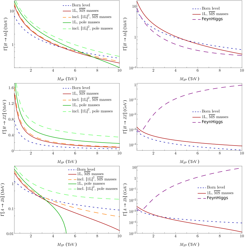
Figure 1: Bosonic two-body decay widths as a function of the heavy Higgs scale in the MSSM at $t_{\beta}=10$: $\Gamma[H\to hh]$, $\Gamma[H\to ZZ]$ and $\Gamma[A\to Zh]$ are displayed in the first, second and third row, respectively.
Left: the born-level amplitude is shown in short-dashed blue, the strict 1L amplitude in solid lines, while the long-dashed curves include a $\text{1L}^{2}$ term. In red, quark masses are set to the running $\overline{\text{MS}}$ value at the Higgs-mass scale; in green, pole masses are employed.
Right: The prediction of FeynHiggs in dashed purple is compared to a selection of curves of the plot on the left-hand side.

In the left column of Fig. 1, the tree-level prediction (short-dashed blue lines) for the channels of Eqs. (1) is shown against $M_{H^{\pm}}$ and compared to our estimates at 1L (red or green solid curves). All curves fall at large $M_{H^{\pm}}$, as expected for $SU(2)_{\mathrm{L}}$-violating channels. We observe that the magnitude of 1L contributions is comparable to that of the born-level amplitudes, indicating that the perturbative series converges slowly. In these conditions, the inclusion of a $\lvert\text{1L}\rvert^{2}$ term (long-dashed curves) seems numerically justified. Nevertheless, such an operation is in general dangerous [33], because the $\lvert\text{1L}\rvert^{2}$ term is a partial 2L contribution which generally contains loose UV-logarithms or uncontrolled symmetry-violating contributions, thus spoiling a quantitative interpretation. Yet, in the case of channels that are purely radiative in the alignment limit, the 1L amplitude is purged of its undesirable features when explicitly applying the limit $\alpha\to\beta-\tfrac{\pi}{2}$: the corresponding piece typically dominates at the numerical level, thus endowing the $\lvert\text{1L}\rvert^{2}$ term with some degree of legitimacy. In any case, comparing the strict 1L widths with their counterparts including a $\lvert\text{1L}\rvert^{2}$ term provides us with a first assessment of the higher-order uncertainty, which reaches as much as $100\%$ for the considered channels.

Another measurement of the large uncertainties at stake at 1L order can be derived from the variation of input in the quark sector: quark masses indeed enter the calculation only in 1L diagrams—both in triangles and self-energy corrections on the external legs—so that a choice of scheme input appears as a higher-order concern. Thus, we compare an on-shell input (green colors) and an $\overline{\text{MS}}$ input with QCD running at the scale of the heavy Higgs masses (red/orange shades). Once again, the variation reaches a $100\%$ magnitude, due to the substantial weakening of Yukawa interactions at high energy. Specializing on the example of $H\to hh$, the contribution of the top quark to the 1L amplitude is of order $g_{Hhh}^{(\text{1L}),t}\approx 3\big{/}\big{(}16\,\sqrt{2}\,\pi\big{)}\,m_{t}^{4}\big{/}(v^{3}\,t_{\beta})\ln^{2}\big{(}M_{H^{\pm}}^{2}\big{/}m_{t}^{2}\big{)}$, implying a quartic dependence on the quark mass input, hence a dramatic dependence on QCD corrections of higher order. In practice, the choice of $\overline{\text{MS}}$ masses at the high scale is expected to properly resum the associated logarithms of UV type, and we correspondingly choose it as our prediction per default. Nevertheless, our discussion should emphasize the impossibility to claim accurate results in the prediction of the bosonic Higgs decays in a 1L analysis: all that is achieved is setting the order of magnitude of the suppressed two-body widths—which is anyway constrained by the symmetries and dimensional analysis.

Despite these bleak conclusions as to the possibility of quantitatively exploiting the bosonic two-body decays of a heavy doublet-Higgs state in the MSSM—they are suppressed and imprecise at 1L—it is crucial to properly estimate their magnitude. On the right-hand side of Fig. 1, still for the channels $H\to hh$, $H\to ZZ$ and $A\to Zh$, we display the tree-level (short dashed blue line) and 1L (solid red line) estimates—identical to the corresponding curves on the left plots—and compare them to the predictions of FeynHiggs-2.18.1 [52, 53, 54, 55, 56, 57, 58, 59] (long dashed purple curves). FeynHiggs employs a partial 1L description of the considered widths, where the tree-level amplitude is rotated with an effective mixing matrix diagonalizing the Higgs-mass system at 1L (and leading 2L) order [60]. In the case of $H\to hh$, this approach does not particularly improve the prediction with respect to a tree-level description (as it is not closer to the full 1L result) but, in view of the sizable uncertainties at stake, it does not notably worsen it either, with, in particular, the correct decoupling behavior at high mass.

However, if we turn to $H\to ZZ$, we observe a problematic growth of the width predicted by FeynHiggs for $M_{H^{\pm}}\gg M_{\text{EW}}$. This response is the direct consequence of the inclusion of a partial 1L order containing $SU(2)_{\mathrm{L}}$-violating pieces that are not controlled by the electroweak v.e.v.: non-decoupling mixing effects actually need to be carefully balanced with the vertex piece—which obviously fails if the latter is not included. We already described this issue in Ref. [33] (see e. g. Fig. 10 in this reference). At this point, one may wonder why the same cause does not result in similarly devastating consequences for $H\to hh$: the reason simply rests with the fact that, in this latter case, the $SU(2)_{\mathrm{L}}$-breaking parameter is already contained within any of the (tree-level) triple-Higgs couplings, i. e. $g_{hhh}$ and $g_{Hhh}$ both scale like $M_{\text{EW}}$; on the contrary, for $H\to ZZ$, the $hZZ$ coupling is unsuppressed, so that a non-decoupling behavior emerges from a call to this quantity via a (non-decoupling) effective mixing. A similar issue appears in $A\to Zh$, with the difference that the non-decoupling mixing is introduced at the level of the SM-like state, through a call to the $SU(2)_{\mathrm{L}}$-conserving $AZH$ coupling.

Finally, we warn the reader against computing off-shell decays $H\to Z^{*}A^{*}$, $A\to Z^{*}H^{*}$, etc., as an integration over off-shell momenta of the final state bosons, after the fashion of Eq. (117) of Ref. [51]. Such expressions are meant to estimate the contribution to four-fermion final states, but the latter involve several destructively interfering diagrams in the case of heavy doublet-Higgs states—with e. g. $Z$-boson emission from a fermion instead of a Higgs line. In our approach, corresponding effects are described in terms of three-body decay widths, e. g. $A\to f\bar{f}\,Z,\,f\bar{f}\,h$, including all tree-level contributions and resumming Sudakov double logarithms (which appear in phase-space integrals) [32]: this results in a less dramatic behavior at high mass, consistent with the $SU(2)_{\mathrm{L}}$ symmetry (contrarily to the off-shell approach). In the case of decays above threshold, such as $A\to Zh$, use of the integration formula is possible, since the on-shell contribution dominates the integral; on the other hand, it also brings little, far from threshold, as compared to a simple on-shell calculation.

2.2 Three-body decays

Order counting sets a three-body width at tree level on the same footing as 1L contributions to a two-body decay. When enough phase space is available, it is thus impossible to perform a complete 1L analysis without studying three-body widths—even after discarding possible contributions with an on-shell internal line, which we count as two body. In the case of fermionic decays, we have shown in Ref. [32] how IR effects (Sudakov logarithms) compensate between three-body and two-body channels, resulting in sizable effects when assessing the full width or branching ratios. Here we focus on final states that strictly involve bosonic particles. For the MSSM, the relevant channels are

• three gauge bosons: $H,\,A\to ZW^{+}W^{-}$; $A\to ZZZ$; $H^{\pm}\to W^{\pm}W^{+}W^{-},\,W^{\pm}ZZ$;

• two gauge bosons and one Higgs boson: $H,\,A\to hW^{+}W^{-}$; $H\to hZZ$; $H^{\pm}\to hW^{\pm}Z$;

• one gauge boson and two Higgs bosons: $A\to hhZ$; $H^{\pm}\to hhW^{\pm}$;

• three Higgs bosons: $H\to hhh$;

where we have neglected $\mathcal{CP}$-violating mixing in the neutral sector (indeed absent at tree level) as well as photon radiation—which we include in the two-body widths so that these are IR-safe with respect to QED.

Contrarily to the two-body decays, many of these channels are $SU(2)_{\mathrm{L}}$-conserving—it is indeed possible to build a doublet out of e. g. three doublets, or one doublet and two triplets. Therefore, no suppression associated to the gauge group arises at the amplitude level, and these channels only entail a three-body phase-space suppression, as well as a $t_{\beta}$-suppression: the corresponding widths then scale linearly with $M_{H^{\pm}}$. For example, in the limit $M_{H^{\pm}}\gg M_{\text{EW}}$, the $H\to hhh$ width is dominated by the contribution of the quartic Higgs coupling:

$$\Gamma[H\to hhh] \stackrel{{\scriptstyle[}}{{M}}_{H^{\pm}}\gg M_{\text{EW}}]{}{\approx}\frac{\lvert g_{Hhhh}\rvert^{2}\,M_{H}}{3072\,\pi^{3}}\,, g_{Hhhh} \stackrel{{\scriptstyle[}}{{\alpha}}\to\beta-\tfrac{\pi}{2}]{}{\approx}\frac{3}{8}\left(g_{1}^{2}+g_{2}^{2}\right)s_{4\beta}\,.$$ (2)

Due to this behavior, the three-body widths involving bosonic final states overtake their two-body counterparts as soon as $M_{H^{\pm}}$ reaches a few TeV.

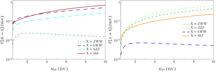
Figure 2: Bosonic three-body decay widths as a function of the heavy Higgs scale in the MSSM at $t_{\beta}=10$: the non-trivial channels are plotted in the cases of a neutral $\mathcal{CP}$-even (left) and $\mathcal{CP}$-odd Higgs (right).

The decays of the neutral heavy-doublet states are shown for illustration in Fig. 2. For each state, $\mathcal{CP}$-even or odd, three channels are $SU(2)_{\mathrm{L}}$-conserving and the associated widths grow linearly with the Higgs mass, while one-channel is $SU(2)_{\mathrm{L}}$-violating, hence suppressed—$\mathcal{CP}$-violating channels vanish. One can easily identify the status of each channel with respect to the $SU(2)_{\mathrm{L}}$ symmetry by checking the existence of a corresponding quartic coupling in the tree-level lagrangian; in such a game, gauge bosons should be identified with their associated Goldstone bosons. Furthermore, the behavior at large $M_{H^{\pm}}$ is mostly determined by these quartic couplings and one deduces the following relations in this limit:

$$\Gamma[H\to hhh] \approx\frac{3}{2}\,\Gamma[H\to hWW] \approx 3\,\Gamma[H\to hZZ]$$

$$\approx\Gamma[A\to ZZZ] \approx\frac{3}{2}\,\Gamma[A\to ZWW] \approx 3\,\Gamma[A\to hhZ]\,.$$ (3)

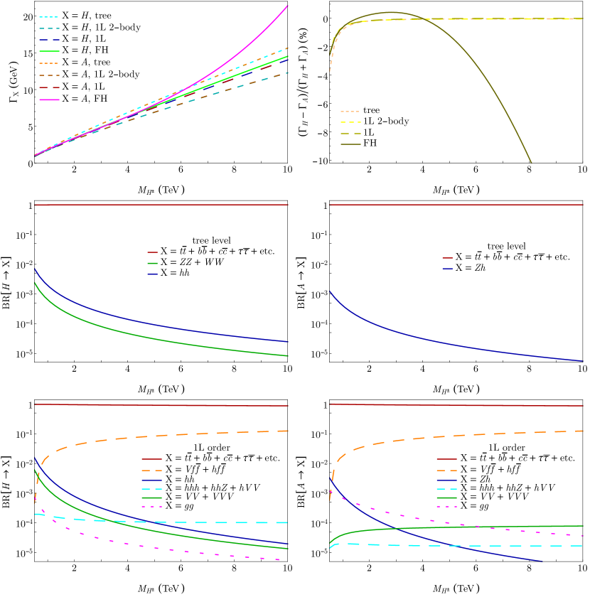
Figure 3: Total widths, magnitude of $SU(2)_{\mathrm{L}}$-breaking, and branching ratios of the neutral heavy Higgs bosons at $t_{\beta}=10$ for the MSSM with a decoupled SUSY sector.
Top Left: Total widths at (QCD+QED-corrected) tree level (short-dashed curves), full 1L (long-dashed curves) and pseudo-widths (sum of 1L-corrected two-body widths; in intermediate dashes). The predictions of FeynHiggs are shown as solid lines.
Top Right: Magnitude that $SU(2)_{\mathrm{L}}$-breaking reaches at the level of the full (pseudo)widths in the various approaches.
Middle: Branching ratios at tree level: fermionic (red), Higgs (blue) and gauge-boson (green) two-body channels.
Bottom: Branching ratios at 1L: three-body fermionic (dashed orange) and bosonic (involving one SM-like Higgs; in dashed cyan) modes, as well as the two-body gluonic rate (dashed magenta) are added to the picture.

The theoretical uncertainty in all these channels can be expected to be sizable (of order $100\%$), since the widths are evaluated at leading order—consistently with the 1L order for two-body decays—and the Higgs potential is known to receive sizable radiative corrections from e. g. Yukawa interactions. Therefore, as for the two-body decays, an evaluation at the considered order only fixes the general magnitude of the three-body widths, without allowing for precision tests.

The decays of the charged Higgs bosons are constrained by the $SU(2)_{\mathrm{L}}$ symmetry to follow a pattern similar to the one of the neutral states, hence these channels exhibit limited novelty. For completeness, we collect a few plots in Appx. A.

2.3 Branching ratios

Having estimated all Higgs decays into SM two-body final states at 1L and three-body final states at tree level, it is possible to consistently evaluate the full widths and branching ratios at this order in scenarios where exotic particles (SUSY) are kinematically inaccessible.

The total widths for the heavy neutral states at $t_{\beta}=10$ are shown in the first row of Fig. 3. As expected from the $SU(2)_{\mathrm{L}}$ symmetry, the predicted widths are comparable for both states, either at the tree level (short-dashed lines) or at the loop level (long-dashed lines). The results of FeynHiggs (solid curves) do not satisfy this property at large $M_{H^{\pm}}$, due to the issues mentioned earlier in the assessment of bosonic decay widths, mainly. In addition, the apparent agreement of the expectations of FeynHiggs for the $\mathcal{CP}$-even state (in green) with our full 1L result is in fact coincidental. Given that FeynHiggs does not consider three-body decays, its predictions should be compared to the pseudo-widths, where only 1L two-body widths are summed (not IR-safe with respect to weak corrections; plotted in dashes of intermediate size): the mismatch is of order $15\%$ and can be explained, in part by the problematic $H\to ZZ,WW$ widths, but also by the contamination of the fermionic widths, on the side of FeynHiggs, by symmetry-violating terms of higher order—we refer the reader to the more detailed discussion of Ref. [33].

The branching ratios at full 1L order are shown in the last row of Fig. 3 and can be compared to the (QCD-corrected) tree-level version (in the middle). The main difference is related to the emergence of the three-body fermionic decays (reaching $\mathcal{O}(10\%)$ at large $M_{H^{\pm}}$; dashed orange lines), which complement the dominant two-body fermionic channels (in solid red). As explained in Ref. [32], these modes essentially involve the radiation of electroweak gauge bosons from the initial Higgs or fermionic final states and are dominated by double logarithms of Sudakov type. Bosonic branching ratios (blue and green curves) remain below percent level—and even permil, for $M_{H^{\pm}}\gtrsim 2$ TeV. The three-body bosonic decays, in particular those modes involving at least one SM-like Higgs boson in the final state (dashed cyan lines), overtake the bosonic two-body decays for $M_{H^{\pm}}\gtrsim 4$ TeV. The linear growth of the associated widths with the Higgs mass ensures that such channels are not further suppressed at large $M_{H^{\pm}}$, contrarily to the $SU(2)_{\mathrm{L}}$-violating two-body modes.

The picture described above remains comparatively stable under variation of $t_{\beta}$, with effects associating to the top Yukawa coupling at low $t_{\beta}$ replacing those of the bottom Yukawa at high $t_{\beta}$. Therefore, as a tribute to the $SU(2)_{\mathrm{L}}$-suppression, bosonic decays of the heavy Higgs states always represent sub-percent-level channels for masses above TeV in the MSSM. Of course, if SUSY final states become accessible, some of them are $SU(2)_{\mathrm{L}}$-conserving and may compete with the SM-fermionic channels.

3 The bosonic Higgs decays in the NMSSM

The presence of singlet degrees of freedom in the NMSSM may noticeably affect the phenomenology of heavy doublet-Higgs states, in particular if these new scalars are kinematically accessible. Indeed, the heavy Higgs bosons may then decay into bosonic final states without breaking the $SU(2)_{\mathrm{L}}$ symmetry, hence opening channels that are competitive with respect to the fermionic ones. Below, we denote the singlet-dominated $\mathcal{CP}$-even and odd scalars as $h_{S}$ and $a_{S}$ respectively.

3.1 Two-body decays

When $h_{S}$ and/or $a_{S}$ take a mass below $M_{H^{\pm}}$, the following two-body decay channels may add up to the MSSM modes:

• decays into two Higgs bosons: $H\to h_{S}h_{S},\,a_{S}a_{S},\,h_{S}h$; $A\to a_{S}h_{S},\,a_{S}h$;

• decays into a Higgs and a gauge boson: $H\to Za_{S}$; $A\to Zh_{S}$; $H^{\pm}\to W^{\pm}h_{S},\,W^{\pm}a_{S}$.

Again, we have assumed $\mathcal{CP}$-conservation for a cleaner classification, but the inclusion of $\mathcal{CP}$-violating mixings does not fundamentally change the situation. Among these new channels, several are again $SU(2)_{\mathrm{L}}$-violating, in substance all those involving only singlet scalars in the final state. However, in contrast to the MSSM, some other decay modes—involving one singlet and one doublet or weak gauge boson (i. e. its Goldstone component)—are $SU(2)_{\mathrm{L}}$-conserving and need not be small in the limit $M_{H^{\pm}}\gg M_{\text{EW}}$ provided the ‘portal’ between singlet and MSSM sectors, i. e. the coupling $\lambda$, is sufficiently intense.

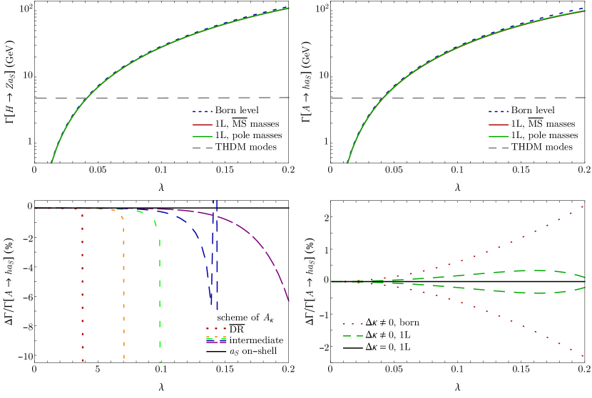
Figure 4: $SU(2)_{\mathrm{L}}$-conserving two-body decays in an NMSSM scenario with $\kappa\stackrel{{\scriptstyle[}}{{]}}{!}{=}\lambda$, $M_{H^{\pm}}=3$ TeV and $M_{a_{S}}=300$ GeV (and $h_{S}$ kinematically inaccessible).
First row: Decay widths $\Gamma[H\to Za_{S}]$ (left) and $\Gamma[A\to ha_{S}]$ (right) as a function of $\lambda$ at tree-level (blue dashed), or 1L (solid curves) with varying definitions of the quark masses (green vs. red).
Second row: Behavior of $\Gamma[A\to ha_{S}]$ under variations of the renormalization scheme for $A_{\kappa}$ (left) or $\kappa$ (right).

We consider a scenario with a comparatively light $\mathcal{CP}$-odd singlet-dominated Higgs boson, setting its mass to $300$ GeV, while $M_{H^{\pm}}\stackrel{{\scriptstyle[}}{{]}}{!}{=}3$ TeV. The SUSY sector (as well as the $\mathcal{CP}$-even singlet) remains decoupled, taking masses in the $10$ TeV range. All input parameters are summarized in Appx. B. The singlet $a_{S}$ primarily decays into fermion pairs, so that the two-body decays of the heavy doublet states that we study below can be understood as the resonant contribution to four-fermion decay channels. In Fig. 4, we vary $\lambda=\kappa$ between low values—where NMSSM effects are negligible and the singlet decouples—and $0.2$ with an active connection between singlet and MSSM sectors. Large radiative corrections to the mass of the singlet pseudoscalar develop for sizable values of $\lambda=\kappa$: this is the simple consequence of the quadratic dependence of scalar masses on the UV spectrum below the SUSY-breaking scale. Technically, this causes complications with the requirement of $M_{a_{S}}\stackrel{{\scriptstyle[}}{{]}}{!}{=}300$ GeV in our original renormalization scheme ($\overline{\text{DR}}$ with the renormalization scale $M_{t}$), as the pseudoscalar mass may be vastly different at the tree level and at 1L. In fact, a ‘tachyonic tree-level syndrome’—see Ref. [35]—emerges as soon as $\lambda\gtrsim 0.04$, making evaluations at the 1L order impossible in this scheme. For this reason, it is convenient to directly work in the renormalization scheme where the counterterm for $A_{\kappa}$ is fixed by an on-shell condition on the mass of $a_{S}$ [35], after the tree-level input is correspondingly translated: the bare $A_{\kappa}$ is kept unchanged in the scheme translation.

We then focus on the two $SU(2)_{\mathrm{L}}$-conserving channels $H\to Za_{S}$ and $A\to ha_{S}$. At the tree level, one may express the widths as

$$\Gamma[H\to Za_{S}] =\frac{M_{H}^{3}\,\lvert g_{HZa_{S}}\rvert^{2}}{64\,\pi\,M_{Z}^{2}}\left[1-\tfrac{2\left(M_{Z}^{2}+M_{a_{S}}^{2}\right)}{M_{H}^{2}}+\tfrac{\left(M_{Z}^{2}-M_{a_{S}}^{2}\right)^{2}}{M_{H}^{4}}\right]^{3/2},$$ (4a)

$$\Gamma[A\to ha_{S}] =\frac{\lvert g_{Aha_{S}}\rvert^{2}}{16\,\pi\,M_{A}}\left[1-\tfrac{2\left(M_{h}^{2}+M_{a_{S}}^{2}\right)}{M_{A}^{2}}+\tfrac{\left(M_{h}^{2}-M_{a_{S}}^{2}\right)^{2}}{M_{A}^{4}}\right]^{1/2}.$$ (4b)

In the $SU(2)_{\mathrm{L}}$ limit with $M_{\text{EW}}\ll M_{H^{\pm}}$, one can directly work out

$$g_{Aha_{S}} \approx\frac{1}{\sqrt{2}}\,\Big{[}3\,\kappa\,\mu_{\text{eff}}-\tfrac{\lambda\,s_{2\beta}}{2\,\mu_{\text{eff}}}\,M_{H^{\pm}}^{2}\Big{]}\,.$$ (5)

Obviously, $g_{Aha_{S}}$ does not vanish and may reach sizable values for $\kappa,\lambda=\mathcal{O}(1)$. This approximation is less immediate for $g_{HZa_{S}}$:

$$g_{HZa_{S}} =\sqrt{g_{1}^{2}+g_{2}^{2}}\,\Big{[}X^{R}_{Hd}\,X^{I}_{a_{S}d}-X^{R}_{Hu}\,X^{I}_{a_{S}u}\Big{]}$$ (6)

with $X^{R,I}_{h_{i}d,u}$ denoting the components of the Higgs field $h_{i}$ with respect to the scalar and pseudoscalar doublet gauge eigenstates; the gauge interaction couples only doublet, not singlet states. Thus, the $H$–$Z$–$a_{S}$ coupling necessarily emerges from singlet–doublet mixing and is $SU(2)_{\mathrm{L}}$-violating. Yet, the prefactor $M_{Z}^{-2}$ in Eq. (4a) shows that the relevant object to consider in the $SU(2)_{\mathrm{L}}$ limit is not $g_{HZa_{S}}$ but $g_{HZa_{S}}\big{/}M_{Z}$. Then, it is convenient to use the connection between gauge and Goldstone couplings, providing the relation $\lvert g_{HZa_{S}}\rvert\big{/}M_{Z}=2\,\lvert g_{HG^{0}a_{S}}\rvert\big{/}(M_{H}^{2}-M_{a_{S}}^{2})$, and to apply the $SU(2)_{\mathrm{L}}$ limit to the Goldstone coupling, i. e.

$$g_{HG^{0}a_{S}} \approx-\frac{1}{\sqrt{2}}\,\Big{[}3\,\kappa\,\mu_{\text{eff}}-\tfrac{\lambda\,s_{2\beta}}{2\,\mu_{\text{eff}}}\,M_{H^{\pm}}^{2}\Big{]}\,.$$ (7)

At this point, we see that the $H\to Za_{S}$ transition actually amounts to a Higgs-to-Higgs decay in the $SU(2)_{\mathrm{L}}$ limit, the $Z$ boson serving as proxy for its Goldstone counterpart. In addition, both channels of Eq. (4) are related by the $SU(2)_{\mathrm{L}}$ symmetry, so that the widths are approximately equal. Radiative corrections are expected to abide by such a symmetry-protected relation.

The decay widths are displayed in the first row of Fig. 4 at the tree level (blue short-dashed line) and at 1L for different definitions of the Yukawa couplings (solid green and red curves). The width corresponding to the sum of the MSSM-like decay modes is also shown (long-dashed gray line) and remains comparatively stable with varying $\kappa=\lambda$. Contrarily to the MSSM case, Higgs-to-Higgs decays are found to dominate over the fermionic modes, provided $\lambda=\kappa$ is sufficiently large. The reason for this behavior is the dependence of $g_{Aha_{S},HG^{0}a_{S}}$ on the scale $\kappa\,\mu_{\text{eff}}$, which can compete with $Y_{f}\,M_{H^{\pm}}$ in the fermionic case (with $Y_{f}$ denoting the Yukawa coupling of the fermion species $f$). Now, focusing on the bosonic decay widths, we observe that these are largely determined by the tree-level amplitudes; 1L corrections only amount to $\mathcal{O}(10\%)$. This again contrasts with the MSSM-like bosonic channels. A fast convergence of the perturbative series is expected and the inclusion of $\lvert\text{1L}\rvert^{2}$ terms appears unjustified (and unpredictive) in such a context. The choice of input for the fermion couplings also appears largely unimportant, with an impact of $\mathcal{O}(1\%)$.

In the second row of Fig. 4, we test the scheme dependence in $\Gamma[A\to ha_{S}]$. In the plot on the left, we study the impact of the treatment of $A_{\kappa}$, considering the variations between a calculation in the scheme with on-shell $M_{a_{S}}$ (black solid line), the original $\overline{\text{DR}}$ scheme (dotted red) and several intermediate choices. The ‘collapse’ of the predictions for non-OS choices is related to the tree-level mass $m_{a_{S}}$ becoming tachyonic; this issue should not distract our attention too much: perturbative calculations are expected to fail for an ill-defined spectrum, and the OS choice is a priori more predictive. More interestingly, in the regime where these schemes are well-defined, their predictions for the decay width do not differ from that obtained with the OS choice by more than a few percent—and this magnitude is reached only in the limit of validity of the non-OS schemes. This confirms the stability of the predicted width under varying definitions of the renormalized $A_{\kappa}$. Yet, given the form of the tree-level couplings—see the paragraph after Eq. (4)—we expect the main uncertainty to originate in the definition of $\kappa$ (or $\mu_{\text{eff}}$). Thus, we also vary the scheme associated with $\kappa$ in the plot on the right-hand side: keeping the bare $\kappa$ unchanged, we consider variations of the renormalized parameter by $\Delta\kappa\approx 3\big{/}(16\,\pi^{2})\,\kappa\,(\lambda^{2}+\kappa^{2})\ln\big{(}M_{\text{SUSY}}^{2}\big{/}M_{t}^{2}\big{)}$, as suggested by the anomalous dimension at 1L. The widths at 1L (dashed green curves) are affected at permil level, at most, against percent for the born level predictions (dotted red lines). This is another sign of the convergence of the perturbative series and we can conclude as to a higher-order uncertainty by at most a few percent on the $SU(2)_{\mathrm{L}}$-conserving channels.

The approximate $SU(2)_{\mathrm{L}}$ relation between the two channels $H\to Za_{S}$ and $A\to ha_{S}$ is roughly satisfied in Fig. 4. Violating effects amount to at most $\mathord{\sim}\,5\%$ at the tree level and $\mathord{\sim}\,10\%$ at 1L (in this specific scenario). This apparently increasing magnitude of the $SU(2)_{\mathrm{L}}$-breaking at 1L should not be over-interpreted: indeed, at this order, three-body decays should be counted at the same level as 1L corrections to the two-body decays. In the next subsection, we will find that the larger three-body decay width of $A$ somewhat compensates the larger suppression of $\Gamma[A\to ha_{S}]$ as compared to $\Gamma[H\to Za_{S}]$.

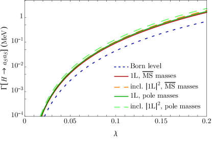
Figure 5: $SU(2)_{\mathrm{L}}$-violating two-body decay width $\Gamma[H\to a_{S}a_{S}]$ in an NMSSM scenario with $\kappa\stackrel{{\scriptstyle[}}{{]}}{!}{=}\lambda$, $M_{H^{\pm}}=3$ TeV and $M_{a_{S}}=300$ GeV (and $h_{S}$ kinematically inaccessible). The convention for the curves is the same as in Sect. 2

In Fig. 5, we consider the $SU(2)_{\mathrm{L}}$-violating decay $H\to a_{S}a_{S}$ (a channel that does not exist in the THDM) in the same scenario as before. As expected, this width is considerably suppressed as compared to those of Fig. 4, though growing with $\lambda=\kappa$. We actually recover features that are largely similar to the MSSM-like Higgs-to-Higgs decays, with a slow convergence of the perturbative series and a sizable dependence on the definition of the SM Yukawa couplings, all hinting at an uncertainty of the order of $100\%$ at 1L. On the other hand, it is always possible to tailor scenarios where a large mixing between $H$ and $h_{S}$ ensures a sizable decay of their admixtures into $a_{S}a_{S}$—exploiting the $SU(2)_{\mathrm{L}}$-conserving decay $h_{S}\to a_{S}a_{S}$; see e. g. Ref. [61]. As the approximate degeneracy between singlet and doublet-dominated states is accidental, such setups are generally fine-tuned.

Attempts at a comparison with the public tools NMSSMCALC [62] and NMSSMCALCEW [45] did not lead to satisfactory results. First, we stress that a preliminary translation of the input is needed, since the renormalization scheme in these codes is different from our choice. Then, electroweak corrections do not seem to produce noticeable IR-like effects in the predictions of NMSSMCALCEW, neither in fermionic nor bosonic two-body modes, which contrasts with our calculation. On the other hand, contrarily to FeynHiggs, we did not observe any obvious violation of the $SU(2)_{\mathrm{L}}$ symmetry in the results of NMSSMCALC and NMSSMCALCEW. Tree-level predictions of bosonic two-body decays are in rough agreement with ours. A deeper understanding of the two implementations of decay widths would thus be needed for a meaningful comparison of the results, which goes beyond our purpose in the current paper.

3.2 Three-body decays

Numerous bosonic three-body final states open up in addition to the THDM ones, when a singlet-dominated (pseudo)scalar is kinematically accessible to the decays of heavy Higgs bosons. It is again necessary to calculate these widths at tree level for a meaningful 1L analysis of the total widths and branching ratios of Higgs bosons. There exist fermionic three-body decay channels involving $h_{S}$ and $a_{S}$ as well: these are typically dominated by the emission of a fermion pair via an off-shell $h$, $G^{0}$ or $G^{\pm}$ in the two-body topology of the previous subsection—see Ref. [32]. We do not study them in detail below.

We consider the three-body decay widths into bosonic final states in the scenario of Fig. 4. As before, we exclude the contributions from resonant internal lines, which are counted in the two-body widths, and keep only off-shell effects at this level. We do not discuss the modes of THDM type here, since they continue to behave in a fashion comparable to that observed in the MSSM. Instead, we focus on final states involving a pseudoscalar $a_{S}$. The results are displayed in Fig. 6. Some channels acquire a sizable width at large $\lambda=\kappa$, which may actually exceed the full width of THDM type. In fact, as could be anticipated, the magnitude of the bosonic three-body widths is comparable (with opposite sign) to that of the 1L effects in the dominant ($SU(2)_{\mathrm{L}}$-conserving) bosonic two-body widths, amounting to $5$–$10\%$ for this specific scenario. Given that the 1L corrections lead to a larger suppression of the two-body width in the pseudoscalar case, which we mentioned earlier, the three-body widths are also more important for $A$, as compared to $H$.

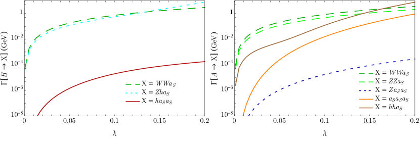
Figure 6: Bosonic three-body decay widths of the heavy doublet-like Higgs bosons, involving $a_{S}$ in the final state, in the scenario of Fig. 4.

This balance between virtual corrections and boson radiation underlines the importance of the IR effects in the three-body channels. Indeed, contrarily to the THDM three-body modes encountered in Sect. 2.2, the widths involving $a_{S}$ are not characterized by the quartic couplings, but by the ‘dressing’ of the leading two-body channels $H\to Za_{S}$, $A\to ha_{S}$ and $H^{\pm}\to W^{\pm}a_{S}$ with radiated light bosons. The latter evidently include electroweak gauge bosons and explain the large contributions to e. g. $H,A\to W^{+}W^{-}a_{S},ZZa_{S}$. From the $SU(2)_{\mathrm{L}}$ perspective, one of the gauge bosons then replaces the associated Goldstone boson while the other behaves vector-like. The width $H\to Zha_{S}$ could be understood in similar terms—at least for moderate values of $\lambda=\kappa$. However, for the larger range of $\lambda=\kappa$, this channel shares some characteristics with $A\to a_{S}hh$, which obviously violates the $SU(2)_{\mathrm{L}}$ symmetry, but emerges as an important channel. The effect at stake here is the radiation of $h$ from the $a_{S}$ line in the soft/collinear regime. Kinematical integration in the off-shell regime close to the $a_{S}$ pole indeed generates a scaling ${\propto}\,m^{-2}_{a_{S}}$ of the decay width, which compensates the suppression by the $SU(2)_{\mathrm{L}}$-breaking trilinear Higgs coupling $a_{S}$–$a_{S}$–$h$: in the aftermath, $\Gamma[A\to a_{S}hh]\propto Mv^{2}/m^{2}_{a_{S}}$, where $M\sim\mu_{\text{eff}},M_{H^{\pm}}$ is one of the large masses of the problem. Therefore, the importance of such $SU(2)_{\mathrm{L}}$-violating channels emerges as a consequence from the accidental fact that $m^{2}_{a_{S}}\sim v^{2}$. Finally, we stress that, from the IR nature of these effects, they largely compensate between virtual and real corrections, so that $SU(2)_{\mathrm{L}}$ remains a pertinent approximate symmetry for the inclusive width.

The precision on these (off-resonance) three-body decay widths calculated at the tree level cannot be very competitive. Given the dominance of IR effects, we can expect the absolute uncertainty to match the residual one in virtual corrections to the two-body decays, i. e. amount to percent level of the two-body widths, or $20$–$50\%$ of the three-body widths. Yet, the general order of magnitude should be under control.

3.3 Branching ratios

With SUSY decays kinematically inaccessible in the considered scenario, we have completed the calculation of all the relevant widths for a 1L evaluation of the total widths and branching ratios of the heavy doublet-Higgs states. The corresponding results for the scenario of Fig. 4 are displayed in Fig. 7.

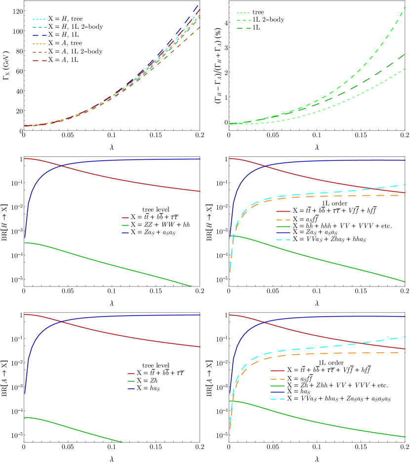
Figure 7: Total widths of the heavy doublet states (first row, left), magnitude that $SU(2)_{\mathrm{L}}$-breaking reaches at the level of the full (pseudo)widths (first row, right), and branching ratios (middle: $\mathcal{CP}$-even Higgs; bottom: $\mathcal{CP}$-odd) at tree-level (left) and 1L order (right) in the scenario of Fig. 4. Decay modes involving $a_{S}$ are depicted in solid blue (two-body), dashed orange (fermionic three-body) and dashed cyan (bosonic three-body).

Focusing on the total width first, we stress the relevance of the three-body channels for a consistent evaluation: the difference between the full widths and the pseudo-widths, considering only two-body channels at 1L, is indeed comparable to the magnitude of the 1L effects, implying an error of full 1L magnitude when the three-body modes are overlooked. In addition, we observe that the magnitude of the $SU(2)_{\mathrm{L}}$-violating effects, measured as the difference between the widths for the scalar and pseudoscalar states (see plot in the top right-hand corner of Fig. 7), remains comparable at the tree level and at 1L, but about doubles when considering the pseudo-widths. This feature is the natural consequence of $SU(2)_{\mathrm{L}}$-violating effects of IR type developing in virtual corrections and Higgs radiation, but compensating between the two.

The general magnitude of the widths considerably varies with the choice of $\lambda=\kappa$, as NMSSM-specific effects range from negligible to dominant. This is most visible at the level of the branching ratios where the THDM fermionic modes (red solid curves) decrease from a significance of about $100\%$ at low $\lambda$ to percent level at $\lambda\approx 0.2$. While the absolute magnitude of the corresponding widths (about $5$ GeV in this scenario) remains constant, the competition of the bosonic Higgs decays involving $a_{S}$ (blue solid line) steadily increases with $\lambda$, resulting in a completely different phenomenology. The general picture qualitatively changes little between the tree level and the 1L order. Only the emergence of the three-body decays diminishes the significance of the two-body modes, substituting them with more complicated final states for a weight of $\mathord{\sim}\,5$–$10\%$. Both fermionic and bosonic three-body modes involving $a_{S}$ become important at large $\lambda$ and may compete in their own right with the THDM modes. As in the MSSM case, however, bosonic final states of THDM type—i. e. involving gauge bosons and the SM-like Higgs boson—remain subdominant in the whole considered range of parameters.

As a concluding note, let us stress that the relative weight of the three-body modes in the decays of heavy Higgs bosons and their mostly IR origin would make it necessary to closely scrutinize the experimental cuts in order to quantitatively exploit a hypothetical measurement of a new Higgs boson and identify the relative importance of the various channels.

4 Conclusions

In this paper, we have shown how the approximate $SU(2)_{\mathrm{L}}$ symmetry in the (experimentally-favored) limit $M_{H^{\pm}}\gg M_{Z}$ severely constrains the decays of the heavy doublet-dominated Higgs bosons of the (N)MSSM. In particular, most available MSSM-like bosonic channels involving two-body final states are purely radiative or $SU(2)_{\mathrm{L}}$-violating, meaning that an evaluation at 1L is only able to estimate the leading order effects, with a very large uncertainty—due to e. g. QCD corrections to fermion loops—persisting in the absolute determination of the widths and branching ratios. The fermionic decay modes thus emerge as the leading contributors to the widths of the heavy-doublet scalars of the MSSM. The bosonic three-body decays are not necessarily $SU(2)_{\mathrm{L}}$-violating and prove competitive with the two-body ones as soon as $M_{H^{\pm}}$ reaches a few TeV. Finally, comparisons with FeynHiggs justify the necessity to modernize this tool in order to study the phenomenology of heavy Higgs bosons.

The situation can drastically change in the presence of comparatively light singlet-dominated states, provided no singlet–doublet decoupling is enforced. Then, two-body decay modes involving Higgs-to-Higgs transitions exist that do not break the electroweak symmetry and may even dominate the decays of the heavy mostly-doublet states. Since no symmetry suppresses the tree-level contributions, such transitions are better controlled by the perturbative expansion (in constrast to their MSSM-like counterparts), with uncertainties at 1L order falling to the percent level. Of course, $SU(2)_{\mathrm{L}}$-violating modes with a large remaining uncertainty at the full 1L order are also present; the exact precision will depend on the details of the scenario. We stressed the importance of IR effects in the 1L corrections (reaching $\mathcal{O}(10\%)$ in the considered example), underlining also that these (virtual) corrections do not necessarily preserve the $SU(2)_{\mathrm{L}}$ symmetry independently from the corresponding tree-level three-body decays (radiation). The latter contribute at the same order as 1L two-body decays and emerge as an essential ingredient for a reliable determination of the widths and branching ratios at the complete 1L order.

With the completion of the evaluation of Higgs decays into SM final states at 1L order, it is possible for us to consistently predict the total widths and branching ratios of Higgs bosons in scenarios where the SUSY spectrum decouples. In the converse case, further competition can be expected from heavy Higgs decays into e. g. electroweakinos, sleptons or even squarks. As such, our results can also be generalized to other models based on a THDM structure.

Appendix A Bosonic decays of a heavy charged Higgs

As dictated by the $SU(2)_{\mathrm{L}}$ symmetry, the decay channels of the charged Higgs in the high-mass regime show little novelty as compared to the case of the neutral heavy-doublet states. From the perspective of electromagnetism, a $W$ boson is always present among the bosonic final states (as this is the only lighter fundamental charged boson).

In the MSSM, the only kinematically accessible bosonic two-body decay at the tree level is $H^{\pm}\to hW^{\pm}$. The channels $H^{\pm}\to ZW^{\pm}$ and $H^{\pm}\to\gamma W^{\pm}$ are purely radiative. In fact, the decay $H^{\pm}\to hW^{\pm}$ is $SU(2)_{\mathrm{L}}$-violating, so that it would also vanish at the tree level in the exact alignment limit. Thus, similarly to the channel $A\to Zh$, the associated width scales like $\Gamma[H^{\pm}\to hW^{\pm}]\propto M^{2}_{\text{EW}}\big{/}M_{H^{\pm}}$, with the $M^{2}_{\text{EW}}\big{/}M_{H^{\pm}}^{2}$ suppression emerging from the mixing in the $\mathcal{CP}$-even sector. As we noted in Sect. 2, a considerable uncertainty persists at the 1L order on such tree-level suppressed channels: this is illustrated by the dispersion of the corresponding predictions in the left plot of Fig. 9, where the choice of scheme for the Yukawa couplings or the inclusion of a 1L² term result in variations of the order of $100\%$. The non-resonant three-body decays in the limit $M_{H^{\pm}}\gg M_{\text{EW}}$ are determined by the quartic Higgs couplings and do not necessarily break the $SU(2)_{\mathrm{L}}$ symmetry. Consequently, they are competitive with the two-body bosonic widths as soon as masses in the few TeV range are considered. The relevant widths are shown in the plot on the right-hand side of Fig. 9.

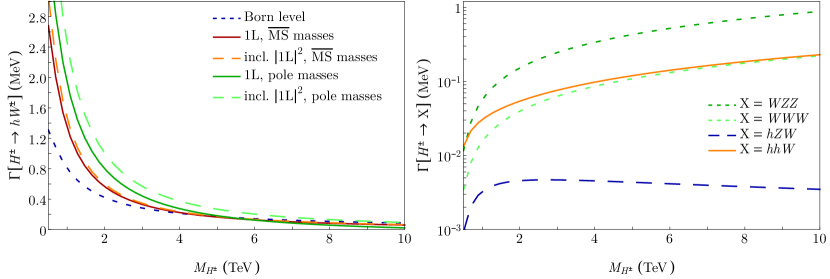
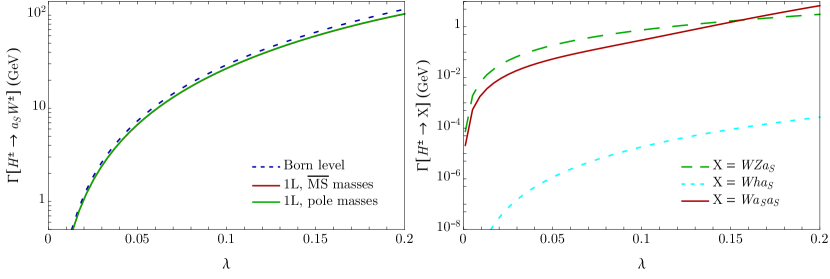
Figure 8: Bosonic Higgs decays of the charged Higgs in the MSSM scenario of Sect. 2.
Left: the two-body width $\Gamma[H^{\pm}\to hW^{\pm}]$ is shown at tree level (dashed blue) and at 1L for two choices of schemes for the Yukawa couplings (pole in green, vs. $\overline{\text{MS}}$ in orange/red), with (long-dash) or without (solid) 1L² terms.
Right: three-body bosonic widths (non-resonant contributions).

Figure 9: Bosonic Higgs decays of the charged Higgs in the NMSSM scenario of Sect. 3.
Left: the two-body width $\Gamma[H^{\pm}\to a_{S}W^{\pm}]$ is shown at tree-level (dashed blue) and at 1L for two choices of schemes for the Yukawa couplings (pole in green, vs. $\overline{\text{MS}}$ in red).
Right: three-body bosonic widths involving $a_{S}$ (non-resonant contributions).

In the NMSSM, the accessibility of comparatively light singlet scalar states modifies the situation with respect to the $SU(2)_{\mathrm{L}}$ symmetry, as unsuppressed channels correspondingly emerge. The latter can completely dominate the charged Higgs width if the singlet–doublet interactions are sufficiently intense. In this case, the tree-level contribution typically determines the widths and a percent-level precision can be expected at the 1L order. The width of the leading two-body channel $H^{\pm}\to W^{\pm}a_{S}$ in the scenario of Sect. 3 is shown on the left-hand side of Fig. 9, with 1L corrections of order $10\%$. Once again, these 1L contributions (for $M_{H^{\pm}}\gg M_{\text{EW},a_{S}}$) involve sizable effects of IR-type, so that (non-resonant) three-body widths of comparable magnitude ($\mathord{\sim}\,10\%$ of the two-body width) balance them at the level of the full width. These three-body channels involving $a_{S}$ in the scenario of Sect. 3 are shown on the right-hand side of Fig. 9. In this case, at large $\lambda=\kappa$, they may compete in magnitude with the MSSM-like channels.

Appendix B Input parameters

The input parameters for the scenarios in Sect. 2 and Sect. 3 are summarized in Tab. 1. The SUSY scale $m_{\mathrm{SUSY}}$ sets the bilinear SUSY-breaking parameters in the sfermion and electroweakino sectors; the gluino-mass parameter is given by $m_{\tilde{g}}$. The tree-level value of $A_{\kappa}$ is fixed according to the on-shell renormalization scheme for the pseudoscalar singlet $a_{s}$ described in Ref. [35]; at $\lambda=\kappa=0$ it is set to $-3$ GeV such that $M_{a_{s}}\sim m_{a_{s}}\sim 300$ GeV. At that point, it also agrees with the input value of $A_{\kappa}$ in the $\overline{\text{DR}}$ scheme at the renormalization scale $\mu_{\mathrm{ren}}=m_{t}=172.3$ GeV.

Table 1: Input parameters for the studied scenarios

	MSSM (Sect. 2)		NMSSM (Sect. 3)
$t_{\beta}$	$10$		$10$
$M_{H^{\pm}}$	$[0.5,10]$	TeV	$3$	TeV
$\mu$	$10$	TeV	$10$	TeV
$m_{\mathrm{SUSY}}$	$10$	TeV	$10$	TeV
$m_{\tilde{g}}$	$10.9$	TeV	$10.9$	TeV
$A_{t}$	$-2.5$	TeV	$-2.5$	TeV
$A_{\tau,b}$	$1$	TeV	$1$	TeV
$\lambda=\kappa$	—		$[0.01,0.20]$
$A_{\kappa}$	—		$-[3.0,7.1]$	GeV

References

- [1] ATLAS Collaboration, CMS Collaboration, Phys. Rev. Lett. 114, 191803 (2015), arXiv:1503.07589.
- [2] CMS Collaboration, A. M. Sirunyan, et al., Phys. Lett. B 805, 135425 (2020), arXiv:2002.06398.
- [3] ATLAS Collaboration, M. Aaboud, et al., Phys. Lett. B 784, 345 (2018), arXiv:1806.00242.
- [4] G. C. Branco, P. M. Ferreira, L. Lavoura, M. N. Rebelo, M. Sher, J. P. Silva, Phys. Rept. 516, 1 (2012), arXiv:1106.0034.
- [5] H. Nilles, Phys. Rept. 110, 1 (1984).
- [6] H. Haber, G. Kane, Phys. Rept. 117, 75 (1985).
- [7] M. Maniatis, Int. J. Mod. Phys. A25, 3505 (2010), arXiv:0906.0777.
- [8] U. Ellwanger, C. Hugonie, A. Teixeira, Phys. Rept. 496, 1 (2010), arXiv:0910.1785.
- [9] J. Kim, H. Nilles, Phys. Lett. B138, 150 (1984).
- [10] CMS Collaboration, (2015), CDS 2055167.
- [11] CMS Collaboration, A. M. Sirunyan, et al., Eur. Phys. J. C79, 421 (2019), arXiv:1809.10733.
- [12] ATLAS Collaboration, G. Aad, et al., Phys. Rev. D 101, 012002 (2020), arXiv:1909.02845.
- [13] M. Misiak, Acta Phys. Polon. B 48, 2173 (2017).
- [14] CMS Collaboration, A. M. Sirunyan, et al., JHEP 09, 007 (2018), arXiv:1803.06553.
- [15] CMS Collaboration, A. M. Sirunyan, et al., JHEP 06, 127 (2018), arXiv:1804.01939, [Erratum: JHEP 03, 128 (2019)].
- [16] CMS Collaboration, A. M. Sirunyan, et al., Phys. Lett. B 798, 134992 (2019), arXiv:1907.03152.
- [17] CMS Collaboration, A. M. Sirunyan, et al., JHEP 04, 171 (2020), arXiv:1908.01115.
- [18] ATLAS Collaboration, G. Aad, et al., Phys. Rev. Lett. 125, 051801 (2020), arXiv:2002.12223.
- [19] ATLAS Collaboration, G. Aad, et al., Eur. Phys. J. C 81, 332 (2021), arXiv:2009.14791.
- [20] ATLAS Collaboration, G. Aad, et al., Phys. Lett. B 822, 136651 (2021), arXiv:2102.13405.
- [21] U. Ellwanger, C. Hugonie, (2022), arXiv:2203.05049.
- [22] CMS Collaboration, A. M. Sirunyan, et al., Eur. Phys. J. C 79, 564 (2019), arXiv:1903.00941.
- [23] CMS Collaboration, A. M. Sirunyan, et al., JHEP 03, 065 (2020), arXiv:1910.11634.
- [24] CMS Collaboration, A. Tumasyan, et al., Phys. Rev. D 105, 032008 (2022), arXiv:2109.06055.
- [25] CMS Collaboration, A. Tumasyan, et al., JHEP 04, 087 (2022), arXiv:2111.13669.
- [26] CMS Collaboration, A. M. Sirunyan, et al., JHEP 03, 055 (2020), arXiv:1911.03781.
- [27] CMS Collaboration, A. Tumasyan, et al., (2022), arXiv:2203.00480.
- [28] ATLAS Collaboration, G. Aad, et al., Eur. Phys. J. C 81, 396 (2021), arXiv:2011.05639.
- [29] ATLAS Collaboration, (2022), arXiv:2207.00230.
- [30] F. Domingo, P. Drechsel, S. Paßehr, Eur. Phys. J. C77, 562 (2017), arXiv:1706.00437.
- [31] F. Domingo, S. Heinemeyer, S. Paßehr, G. Weiglein, Eur. Phys. J. C78, 942 (2018), arXiv:1807.06322.
- [32] F. Domingo, S. Paßehr, Eur. Phys. J. C79, 905 (2019), arXiv:1907.05468.
- [33] F. Domingo, S. Paßehr, Eur. Phys. J. C 80, 1124 (2020), arXiv:2007.11010.
- [34] F. Domingo, S. Paßehr, Eur. Phys. J. C 81, 661 (2021), arXiv:2105.01139.
- [35] F. Domingo, S. Paßehr, Eur. Phys. J. C 82, 98 (2022), arXiv:2109.00585.
- [36] T. Graf, R. Gröber, M. Mühlleitner, H. Rzehak, K. Walz, JHEP 10, 122 (2012), arXiv:1206.6806.
- [37] M. Mühlleitner, D. T. Nhung, H. Rzehak, K. Walz, JHEP 05, 128 (2015), arXiv:1412.0918.
- [38] M. Goodsell, K. Nickel, F. Staub, Phys. Rev. D91, 035021 (2015), arXiv:1411.4665.
- [39] M. Goodsell, K. Nickel, F. Staub, Eur. Phys. J. C75, 290 (2015), arXiv:1503.03098.
- [40] M. D. Goodsell, F. Staub, Eur. Phys. J. C77, 46 (2017), arXiv:1604.05335.
- [41] M. D. Goodsell, S. Paßehr, Eur. Phys. J. C 80, 417 (2020), arXiv:1910.02094.
- [42] T. N. Dao, M. Gabelmann, M. Mühlleitner, H. Rzehak, (2021), arXiv:2106.06990.
- [43] M. Goodsell, S. Liebler, F. Staub, Eur. Phys. J. C77, 758 (2017), arXiv:1703.09237.
- [44] G. Bélanger, V. Bizouard, F. Boudjema, G. Chalons, Phys. Rev. D96, 015040 (2017), arXiv:1705.02209.
- [45] J. Baglio, T. N. Dao, M. Mühlleitner, Eur. Phys. J. C 80, 960 (2020), arXiv:1907.12060.
- [46] T. N. Dao, M. Mühlleitner, S. Patel, K. Sakurai, Eur. Phys. J. C 81, 340 (2021), arXiv:2012.14889.
- [47] J. Braathen, M. D. Goodsell, S. Paßehr, E. Pinsard, Eur. Phys. J. C 81, 498 (2021), arXiv:2103.06773.
- [48] M. Spira, A. Djouadi, D. Graudenz, P. Zerwas, Nucl. Phys. B453, 17 (1995), arXiv:hep-ph/9504378.
- [49] P. A. Baikov, K. G. Chetyrkin, Phys. Rev. Lett. 97, 061803 (2006), arXiv:hep-ph/0604194.
- [50] M. Mühlleitner, M. Spira, Nucl. Phys. B790, 1 (2008), arXiv:hep-ph/0612254.
- [51] M. Spira, Prog. Part. Nucl. Phys. 95, 98 (2017), arXiv:1612.07651.
- [52] S. Heinemeyer, W. Hollik, G. Weiglein, Comput. Phys. Commun. 124, 76 (2000), arXiv:hep-ph/9812320.
- [53] S. Heinemeyer, W. Hollik, G. Weiglein, Eur. Phys. J. C9, 343 (1999), arXiv:hep-ph/9812472.
- [54] G. Degrassi, S. Heinemeyer, W. Hollik, P. Slavich, G. Weiglein, Eur. Phys. J. C28, 133 (2003), arXiv:hep-ph/0212020.
- [55] M. Frank, T. Hahn, S. Heinemeyer, W. Hollik, H. Rzehak, G. Weiglein, JHEP 0702, 047 (2007), arXiv:hep-ph/0611326.
- [56] T. Hahn, S. Heinemeyer, W. Hollik, H. Rzehak, G. Weiglein, Phys. Rev. Lett. 112, 141801 (2014), arXiv:1312.4937.
- [57] H. Bahl, W. Hollik, Eur. Phys. J. C76, 499 (2016), arXiv:1608.01880.
- [58] H. Bahl, S. Heinemeyer, W. Hollik, G. Weiglein, Eur. Phys. J. C78, 57 (2018), arXiv:1706.00346.
- [59] H. Bahl, T. Hahn, S. Heinemeyer, W. Hollik, S. Paßehr, H. Rzehak, G. Weiglein, Comput. Phys. Commun. 249, 107099 (2020), arXiv:1811.09073.
- [60] K. Williams, H. Rzehak, G. Weiglein, Eur. Phys. J. C71, 1669 (2011), arXiv:1103.1335.
- [61] F. Domingo, S. Heinemeyer, J. Kim, K. Rolbiecki, Eur. Phys. J. C76, 249 (2016), arXiv:1602.07691.
- [62] J. Baglio, R. Gröber, M. Mühlleitner, D. Nhung, H. Rzehak, M. Spira, J. Streicher, K. Walz, Comput. Phys. Commun. 185, 3372 (2014), arXiv:1312.4788.