The Far-Ultraviolet Continuum Slope as a Lyman Continuum Escape Estimator at High-redshift

Abstract

Most of the hydrogen in the intergalactic medium (IGM) was rapidly ionized at high-redshifts. While observations have established that reionization occurred, observational constraints on the emissivity of ionizing photons at high-redshift remains elusive. Here, we present a new analysis of the Low-redshift Lyman Continuum Survey (LzLCS) and archival observations, a combined sample of 89 star-forming galaxies at redshifts near 0.3 with Hubble Space Telescope observations of their ionizing continua (or Lyman Continuum, LyC). We find a strong ($6\sigma$ significant) inverse correlation between the continuum slope at 1550 Å (defined as F${}_{\lambda}\propto\lambda^{\beta^{1550}_{\rm obs}}$) and both the LyC escape fraction ($f_{\rm esc,LyC}$) and $f_{\rm esc,LyC}$ times the ionizing photon production efficiency ($\xi_{\rm ion}$). On average, galaxies with redder continuum slopes have smaller $f_{\rm esc,LyC}$ than galaxies with bluer slopes due to the higher dust attenuation in redder galaxies. More than 5% (20%) of the LyC emission escapes galaxies with $\beta_{\rm obs}^{1550}$ $<-2.1$ (-2.6). We find strong correlations between $\beta_{\rm obs}^{1550}$ and the gas-phase ionization ([O iii]/[O ii] flux ratio; at 7.5$\sigma$ significance), galaxy stellar mass (at 5.9$\sigma$), the gas-phase metallicity (at 4.6$\sigma$), and the observed FUV absolute magnitude (at 3.4$\sigma$). Using previous observations of $\beta_{\rm obs}^{1550}$ at high-redshift, we estimate the evolution of $f_{\rm esc,LyC}$ with both redshift and galaxy magnitude. The LzLCS observations suggest that fainter and lower mass galaxies dominate the ionizing photon budget at higher redshift, possibly due to their rapidly evolving metal and dust content. Finally, we use our correlation between $\beta_{\rm obs}^{1550}$ and $f_{\rm esc,LyC}$ $\times$ $\xi_{\rm ion}$ to predict the ionizing emissivity of galaxies during the epoch of reionization. Our estimated emissivities match IGM observations, and suggest that star-forming galaxies emit sufficient LyC photons into the IGM to exceed recombinations near redshifts of 7–8.

1 Introduction

Observations of high-redshift quasars indicate that the intergalactic medium (IGM) underwent a large-scale phase change near $z\sim 5-10$ (Becker et al., 2001; Fan et al., 2006; Bañados et al., 2018; Becker et al., 2021). At these redshifts, gas between galaxies rapidly transitions from being largely neutral to being largely ionized. This “epoch of reionization” seeds the subsequent large-scale structure of the Universe (Gnedin, 2000), impacts the interpretation of the cosmic microwave background radiation (Planck Collaboration et al., 2016), and sets the IGM temperature (Miralda-Escudé & Rees, 1994).

Determining the structure and evolution of reionization requires uncovering what emitted the first hydrogen ionizing, or Lyman Continuum (LyC), photons. Whether the sources of ionizing photons are broadly distributed spatially, or more concentrated impacts the morphology of reionzation (Kulkarni et al., 2019a). The timing and duration of reionzation strongly depend upon whether massive stars, active galactic nuclei (AGN), or evolved stellar remnants are key contributors to reionization (Robertson et al., 2013; Madau & Dickinson, 2014; Robertson et al., 2015; Rosdahl et al., 2018).

The initial debate on the sources of reionization centered around whether AGN or star-forming galaxies reionized the early IGM (Ouchi et al., 2009; Hopkins et al., 2008; Faucher-Giguère et al., 2009; Finkelstein et al., 2012; Robertson et al., 2013; Madau & Haardt, 2015). However, current observations and simulations find too few active galactic nuclei during the epoch of reionization to dominate the ionizing photon budget (Fontanot et al., 2007; Trebitsch et al., 2017; Ricci et al., 2017; Matsuoka et al., 2018; Kulkarni et al., 2019b; Shen et al., 2020; Faucher-Giguère, 2020; Dayal et al., 2020; Yung et al., 2021; Trebitsch et al., 2021; Jiang et al., 2022). The observational landscape of high-redshift AGN may dramatically change as the sensitivity of the JWST opens a new window onto the epoch of reionization, but the current observational picture suggests that star-forming galaxies reionized the IGM. Coupled with the recent success of LyC observations from local galaxies (see below), the current debate has shifted to whether bright massive galaxies that are clustered in over densities or widely-distributed low-mass galaxies emitted the requisite ionizing photons (Finkelstein et al., 2019; Naidu et al., 2020; Mason et al., 2019; Finkelstein et al., 2021; Naidu et al., 2022; Matthee et al., 2021).

Determining the ionizing emissivity ($\dot{n}_{\rm ion}$) of a given population (e.g. AGN or star-forming) at high redshift requires estimating the number density of sources and the number of ionizing photons that each source emits into the IGM. This can be cast in terms of the UV luminosity density ($\rho_{\rm UV}$), the production efficiency of ionizing photons ($\xi_{\rm ion}$, or the number of ionizing photons per FUV luminosity), and the fraction of LyC photons that escape each source ($f_{\rm esc,LyC}$). Numerically, $\dot{n}_{\rm ion}$ is the product of these three quantities as

$$\dot{n}_{\rm ion}=\rho_{\rm UV}\times\xi_{\rm ion}\times f_{\rm esc,LyC}.$$ (1)

All of these quantities likely vary with redshift and with galaxy property (e.g. stellar mass or far-ultraviolet absolute magnitude), but each quantity can in principle be estimated from galaxies in the epoch of reionization.

Deep Hubble Space Telescope observations have estimated $\rho_{\rm UV}$ out to redshifts as high as 10 (Bouwens et al., 2015; Finkelstein et al., 2015; McLeod et al., 2016; Livermore et al., 2017; Mehta et al., 2017; Atek et al., 2018; Oesch et al., 2018; Yue et al., 2018; Bouwens et al., 2021; Bouwens et al., 2022). Similarly, deep rest-frame far-ultraviolet (FUV) spectroscopy (Stark et al., 2015; Mainali et al., 2018; Tang et al., 2019; Hutchison et al., 2019) and Spitzer rest-frame optical (Bouwens et al., 2016; De Barros et al., 2019; Endsley et al., 2021) observations of epoch of reionization-era systems find hard radiation fields indicative of high $\xi_{\rm ion}$ ($\sim 10^{25.3-26}$ [s^-1/erg s^-1 Hz^-1]). Combined, these observations hint that star-forming galaxies can reionize the IGM if $f_{\rm esc,LyC}$ $>5-20$% (Ouchi et al., 2009; Robertson et al., 2013; Robertson et al., 2015; Finkelstein et al., 2019; Mason et al., 2019; Naidu et al., 2020; Naidu et al., 2022; Matthee et al., 2021).

The neutral IGM precludes direct LyC detections at $z>4$ in a statistical sense (Inoue et al., 2014; Becker et al., 2021), outside of rare ionized regions (Endsley et al., 2021; Endsley & Stark, 2022). However, $f_{\rm esc,LyC}$ can be directly measured at $z<4$ (Bergvall et al., 2006; Leitet et al., 2011; Borthakur et al., 2014; Izotov et al., 2016a, b; Vanzella et al., 2016; Leitherer et al., 2016; Shapley et al., 2016; Izotov et al., 2018a; Izotov et al., 2018b; Steidel et al., 2018; Fletcher et al., 2019; Wang et al., 2019; Rivera-Thorsen et al., 2019; Ji et al., 2020; Izotov et al., 2021; Davis et al., 2021; Marques-Chaves et al., 2021; Xu et al., 2022). To overcome the neutral high-redshift IGM, recent work has correlated indirect observables with $f_{\rm esc,LyC}$ at these low redshifts. Tentative correlations, with appreciable scatter and significant non-detections (Rutkowski et al., 2017), have been found between the Ly$\alpha$ emission properties (Verhamme et al., 2015; Rivera-Thorsen et al., 2017; Izotov et al., 2018b; Steidel et al., 2018; Gazagnes et al., 2020; Izotov et al., 2021), ISM absorption properties (Reddy et al., 2016; Chisholm et al., 2017; Gazagnes et al., 2018; Chisholm et al., 2018; Steidel et al., 2018), Mg ii resonant emission lines (Henry et al., 2018; Chisholm et al., 2020; Witstok et al., 2021; Xu et al., 2022), and optical emission line ratios (Nakajima & Ouchi, 2014; Jaskot & Oey, 2014; Wang et al., 2019). Recent simulations have tested these indirect indicators and have found modest efficacy with strong impacts from geometry and dust (Mauerhofer et al., 2021; Katz et al., 2022). These first glimpses of small samples of LyC emitters at lower redshifts provide a blueprint to estimate $f_{\rm esc,LyC}$ during the epoch of reionization.

While there are promising LyC tracers, LyC emitting galaxies have been elusive and the sample sizes of confirmed LyC detections was still modest. The small LyC samples may obscure trends or introduce false trends in LyC escape detections. The Low-Redshift Lyman Continuum Survey (LzLCS; Flury et al., 2022a) is a 134 orbit Hubble Space Telescope project that used the Cosmic Origins Spectrograph (COS) to target 66 new $z\sim 0.3$ LyC emitting candidates. The LzLCS was developed to explore the galaxy parameter range relevant to cosmic reionization to assess the validity of a variety of indirect LyC tracers (Flury et al., 2022a). The LzLCS sample has a dynamic range in three purported LyC diagnostics: H$\beta$ equivalent width, the [O iii]/[O ii] flux ratio, and the slope of the FUV stellar continuum ($\beta$). This range of parameters stringently tests indirect trends of LyC escape, establishing whether they scale with $f_{\rm esc,LyC}$ at low-redshifts (Flury et al., 2022b).

The LzLCS is a resounding success. Combined with archival HST/COS observations, the full LzLCS plus archival survey contains 89 LyC observations. More than half, 55%, of these galaxies have LyC emission detected above the background at the $>$97.7% confidence level and the other 45% have robust upper limits (Flury et al., 2022a). This provides a definitive local sample to explore indirect diagnostics in $f_{\rm esc,LyC}$. Flury et al. (2022b) found that many of the classical LyC diagnostics have appreciable scatter, but in general more highly ionized, vigorously star-forming, and compact galaxies are more likely to emit ionizing photons. The Ly$\alpha$ equivalent width, escape fraction, and velocity separation strongly correlate with $f_{\rm esc,LyC}$ (Flury et al., 2022b). LyC emitters within the LzLCS are deficient in low-ionization optical metal emission lines, specifically [S ii], indicating that LyC emitters are relatively deficient in low-ionization gas (Wang et al., 2021). The COS FUV spectral range also provides invaluable probes of the H i in the galaxies with the Lyman Series absorption lines. These H i lines suggest that LyC emission escapes through regions in the galaxy with low neutral gas covering fraction and low dust attenuation (Saldana-Lopez et al., 2022). As such, $f_{\rm esc,LyC}$ can be robustly predicted using the combination of H i absorption and dust attenuation.

Here we extend the previous LzLCS work to a detailed analysis of the FUV spectral slope, $\beta_{\rm obs}^{1550}$, derived from stellar population fits and their relation to the $f_{\rm esc,LyC}$. $\beta_{\rm obs}^{1550}$ traces both the stellar population parameters and the dust attenuation in the LzLCS galaxies, and has been theoretically predicted to correlate with $f_{\rm esc,LyC}$ (e.g., Zackrisson et al., 2013). In section 2 we describe the LzLCS sample and observations. section 3 describes the modeling of the FUV stellar continua, and the derivation of stellar continuum properties. We explore correlations with $\beta_{\rm obs}^{1550}$ (section 4) before introducing the strong relation between $\beta_{\rm obs}^{1550}$ and the $f_{\rm esc,LyC}$ (section 5). The physical picture presented by the $\beta_{\rm obs}^{1550}$-$f_{\rm esc,LyC}$ relation is explored in section 6. We conclude in section 7 by using the $\beta_{\rm obs}^{1550}$-$f_{\rm esc,LyC}$ relation to make predictions for $f_{\rm esc,LyC}$  and $\dot{n}_{\rm ion}$ during the epoch of reionzation to predict which galaxies heavily contribute to reionization. In Appendix A we also detail the impact of different assumed extinction laws. Throughout this paper we use AB magnitudes; a standard cosmology with $H_{0}$ = 70 km s^-1, $\Omega_{m}$ = 0.3, and $\Omega_{\Lambda}$ = 0.7; and stellar metallicities that are relative to a solar value of 0.02.

2 Observations

Here we describe the observations of the local LyC emitting galaxies. We use three subsets of data: the Low-redshift Lyman Continuum Survey (subsection 2.1), archival observations of 23 LyC emitters (subsection 2.2; Izotov et al., 2016b, a; Izotov et al., 2018a; Izotov et al., 2018b; Wang et al., 2019; Izotov et al., 2021), and finally a coaddition of all the LzLCS plus archival spectra. We combine the LzLCS and archival samples into one cohesive sample that we refer to as the full LzLCS sample.

2.1 The LzLCS

We use data from the Low-redshift Lyman Continuum Survey (LzLCS; PI: Jaskot, HST Project ID: 15626; Flury et al., 2022a). The LzLCS is a large Hubble Space Telescope program consisting of 134 orbits targeting 66 star-forming galaxies at redshifts between 0.219–0.431. We chose these redshifts to shift the LyC onto the sensitive spectral portion of the COS detector. These 66 galaxies were selected using optical observations from the 16th Data Release of the Sloan Digital Sky Survey (SDSS; Ahumada et al., 2020), and non-ionizing FUV observations from the GALaxy Evolution eXplorer (GALEX; Martin et al., 2005). The LzLCS was designed to test the efficacy of three potential indicators of LyC escape by creating three separate, but overlapping, samples with a large dynamic range of star formation rate surface density (as probed by the $\Sigma_{\rm SFR}$ measured from H$\beta$ emission), nebular ionization state (as probed by the [O iii]/[O ii] optical emission line ratio), and UV continuum slopes (as measured by the GALEX FUV-NUV slope). The resultant sample probes the full property range expected at high-redshift to test the impact of various properties on $f_{\rm esc,LyC}$.

The details of the data reduction are given in Flury et al. (2022a), but here we summarize the procedure. Each galaxy was observed for between 1–5 orbits with the low-resolution G140L grating of the Cosmic Origins Spectrograph (COS; Green et al., 2012). We used the G140L/800 mode (Redwine et al., 2016), which has observed wavelength coverage between 800-1950Å at a spectral resolution of $R\sim 1000$ at 1100Å. This extremely blue-optimized COS configuration places the LyC onto the sensitive portion of the COS detector and affords rest-frame coverage of 600-1480Å for the median redshift of the LzLCS. In addition to the crucial LyC, the LzLCS observations sample the very blue of the non-ionizing FUV continuum.

The COS observations were flat-fielded, wavelength calibrated, and flux calibrated using CALCOS v3.3.9. The individual exposures were co-added in the raw counts using faintcos (Makan et al., 2021). faintcos directly uses many time-baselines of archival COS observations to re-estimate the dark current, uses the scattered light model from Worseck et al. (2016) to improve the flux calibration at faint flux levels, and accounts for the Poisson uncertainties of the photon-counting COS FUV detector. Flury et al. (2022a) also details the accounting of the geocoronal emission to address possible LyC contamination.

The individual COS spectra were corrected for the foreground Milky Way reddening using the Green et al. (2018) dust maps and the Milky Way extinction curve (Fitzpatrick, 1999). We then measured the observed counts in 20Å regions in the rest-frame LyC. The inferred LyC counts and background levels, along with a Poisson distribution, are used in a survival function to determine the probability that the signal arises through chance realizations from the background distribution. If the survival analysis confirms that the flux is above the background counts at the $>97.7$% confidence level, we classify these as LyC detections, and we refer to them as galaxies with “Detected LyC” for the rest of the paper. We also checked the 2-dimensional spectra by eye to ensure that these detections are not spikes in background counts. The galaxies with LyC flux $<97.7$% above the background are called “non-detected LyC” galaxies throughout this paper. These detection thresholds do not mean that the non-detected galaxies do not emit LyC photons, rather the LyC is not significantly detected given the observed backgrounds. Of the 66 galaxies in the LzLCS, 35 have LyC photons detected at $>97.7$% confidence level.

All LzLCS galaxies have archival SDSS optical spectroscopy (Ahumada et al., 2020). These optical emission lines describe the nebular emission line properties and the gaseous conditions. In section 4, we use these emission lines to explore the relation between nebular conditions and the FUV slope. The nebular reddening values, E(B-V)_gas, are determined in an iterative way where the temperature, density, and extinction (assuming the extinction law from Cardelli et al., 1989) are all iterated until the Balmer emission line flux ratios converge (Flury et al., 2022a). In this way, the temperature and density dependence of the Balmer line ratios are accounted for when determining the internal reddening of the galaxies. The nebular electron temperatures (T_e) are directly measured using the [O iii] 4363 Å auroral line for 54 galaxies. The extinction-corrected emission line fluxes are used to determine line-ratios of certain ions (e.g., [O iii] 5007/[O ii] 3726+3729 Å) which serve as a proxy of the gas ionization. Finally, the [S ii] 6717, 6731 Å Å doublet is used to determine the electron density of the gas and the metallicities are measured from the inferred electron temperatures, densities, and attenuation-corrected fluxes. Metallicities of the 12 galaxies without auroral line detections were determined using the strong-line calibration from Pilyugin et al. (2006).

2.2 Archival Data

In combination with the LzLCS, we also use a compilation of 23 galaxies drawn from the literature (Izotov et al., 2016b, a; Izotov et al., 2018a; Izotov et al., 2018b; Wang et al., 2019; Izotov et al., 2021). These galaxies are also observed with COS on HST and their reduction is handled in the same exact way as the rest of the LzLCS. This produces a homogeneous sample of 89 galaxies with LyC observations. Of the archival sample, we detect the LyC above the background at a $>$97.7% confidence level in 15 galaxies. This leads to a total of 50 detections in the full LzLCS plus archive sample.

2.3 Spectral co-additions

In order to illustrate the changes of the stellar features at high significance, we also coadd the spectra to increase the resultant signal-to-noise. The details of this process are found in Flury et al. (in preparation). We coadded all of the full LzLCS sample and made two separate composite spectra: (1) of all galaxies with detected LyC emission and (2) of all galaxies without LyC detections. We take care to mask intervening ISM, Milky Way absorption features, as well as the Ly$\alpha$ and O i 1302 and 1306 Å geocoronal emission lines, in each individual galaxy before co-adding the spectra. The individual spectra are then normalized to the median flux density at 1100 Å and the spectra are coadded in the rest-frame. The uncertainties on the flux density are determined by bootstrapping the individual fluxes that comprise the stack. This high signal-to-noise stack is used in the next section to compare to stellar population synthesis models.

3 Stellar Continuum Fitting

3.1 Fitting procedure

In Saldana-Lopez et al. (2022), we fit the observed stellar continua of the LzLCS and archival samples, following Chisholm et al. (2019), as a linear combination of multiple single age, single metallicity stellar continuum models (see subsection 3.2 for a discussion of the models used). Here, we use those continuum fits and briefly describe the fitting procedure, but refer the reader to Chisholm et al. (2019) and Saldana-Lopez et al. (2022) for in depth discussions on the procedure and the associated assumptions.

We assume that the observed stellar continuum ($F(\lambda)$) is the product of the intrinsic stellar continuum ($F_{i}(\lambda)$) attenuated by a uniform dust screen. The treatment of the dust screen geometry impacts the interpretation of the stellar continuum fitting (Calzetti et al., 1994; Vasei et al., 2016; Gazagnes et al., 2018), but it is challenging to distinguish the appropriate model with many degenerate effects (Calzetti, 2013). Therefore, we assume a uniform dust screen. The intrinsic flux is modeled as a linear combination of a set of $j$ stellar continuum models with different ages and metallicities ($M_{j}(\lambda)$) times a weight ($X_{j}$) that describes the contribution of each $M_{j}$ to the total $F_{i}(\lambda)$. These $X_{j}$ can have values greater than or equal to 0. Mathematically, this is defined as

$$F(\lambda)=F_{i}(\lambda)\times 10^{-0.4{\rm E(B-V)}k(\lambda)}=10^{-0.4{\rm E(B-V)}k(\lambda)}\Sigma_{j}\left(X_{j}\times M_{j}(\lambda)\right).$$ (2)

We use the reformulated Reddy et al. (2016) attenuation curves that is prescribed with a dust law, k$(\lambda$), and the continuum color excess (E(B-V)). The Reddy et al. (2016) law is similar in shape to the Calzetti et al. (2000) law, but with a lower normalization (the E(B-V) is inferred to be 0.008 mag redder than the Calzetti attenuation law; see figure 5 of Reddy et al., 2016). In Appendix A, we introduce analytic relations to convert between different attenuation laws. The Reddy et al. (2016) law is observationally defined in the observed wavelength regime down to 950Å  while the Calzetti et al. (2000) is only defined to 1250Å. We use the python package LMFIT (Newville et al., 2014) to determine the best-fit values for each of the $X_{j}$ linear coefficients and the E(B-V) values.

To fit the spectra, we place the galaxies into the rest-frame using the SDSS redshifts (Ahumada et al., 2020) and normalize the flux density to the median rest-frame flux density between 1070–1100 Å. The rest-frame FUV contains many non-stellar features, such as foreground Milky Way absorption lines, geocoronal emission features, and ISM absorption lines from the targeted galaxies. These features do not arise from the stellar populations and should not be included in the fitting process. We mask these regions of the spectra by hand. We also mask out regions of low signal-to-noise ratios (less than one) to avoid fitting continuum noise. We tested whether including low signal-to-noise data improves the fitting and found a poorer match between models and observations when including lower quality data. We fit the rest-frame wavelengths between 950-1345 Å to avoid heavy contamination of the Lyman Series lines at bluer wavelengths. The median reduced $\chi^{2}$ is 1.08 (Saldana-Lopez et al., 2022). Detailed comparisons of models and individual spectra are given in figures 1-2 of Saldana-Lopez et al. (2022).

Errors on the stellar continuum fits were calculated by modulating the observed flux density with the error spectra at each pixel, refitting the spectrum, and then tabulating the associated stellar continuum properties (Saldana-Lopez et al., 2022). We repeated this process 500 times for each galaxy to build a sample distribution of stellar population fits. We measured the standard deviations of these Monte Carlo distributions to determine the standard deviations on all fitted parameters ($X_{j}$ and E(B-V)) and the other inferred parameters.

3.2 Stellar continuum models

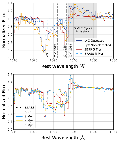
Figure 1: Upper Panel: The O vi 1032,1038 ÅÅ doublet stellar wind feature for the co-added full sample of LzLCS plus archival galaxies with LyC detections (blue line) and non-detections of the LyC (gold line). The O vi profile has two main components: broad absorption that extends to 1025 Å and broad emission that extends out to 1050 Å. Strong ISM absorption lines are marked by gray vertical dashed lines. Overlaid are two fully theoretical stellar population models from starburst99 (red line) and bpass (blue dotted line), with similar parameters as the median of our fits (age of 5 Myr and metallicity of 0.2 Z_⊙). The bpass model does not match either the observed P-Cygni absorption nor emission, while the starburst99 model matches the absorption profile but not the full extent of the emission. Lower Panel: Stellar population synthesis models at a range of ages: 3 (blue), 4 (gold), and 5 Myr (red). We include both starburst99 (solid lines) and bpass (dotted lines) models. The O vi profile weakens with increasing age for the starburst99 models, indicating that O vi is sensitive to the stellar population age. The O vi region of the bpass models hardly varies with stellar population age. The strong O vi P-Cygni profile suggests that the LzLCS galaxies have very young stellar populations.

To fit the observed LzLCS FUV spectra, we use fully theoretical single-age bursts of star formation to model the very young stellar continua. As in Saldana-Lopez et al. (2022), we include stellar models with a range of single ages of 1, 2, 3, 4, 5, 8, and 10 Myr with metallicities in the range of 0.05, 0.2, 0.4, and 1.0 Z_⊙. These ages were carefully chosen to sample the spectral variations of the FUV stellar continuum (Chisholm et al., 2019). Each stellar model (defined by an age and metallicity) includes a modeling of the nebular continuum by placing each single-age model into cloudy v17.0 (Ferland et al., 2017), assuming that all of the ionizing photons are absorbed by the nebular gas, and tabulating the resultant nebular continuum. The nebular continuum is then added back to original stellar model (Chisholm et al., 2019). The nebular continuum does not heavily affect the wavelengths covered by the LzLCS observations, but contributes to the continuum slope at 1550 Å (Raiter et al., 2010). We tested including older ages (up to 40 Myr) and found that they do not significantly change the inferred stellar population properties of the very young LzLCS spectra. However, the fully theoretical, high-resolution starburst99 models do not densely sample the H-R diagram at effective temperatures below 15,000 K (Leitherer et al., 2010). The cooler, high-resolution models have artificially bluer continuum slopes that makes older stellar populations appear much bluer than expected for their temperatures. A similar resolution issue is found in the bpass models (Chisholm et al., 2019). Thus, we choose the maximum model age range of 10 Myr that includes high-resolution models that accurately probe the stellar spectral features and the continuum shape. We fully describe the observed stellar continuum using 28 free parameters (each $X_{j}$) for the stellar models and one for the dust (for a total of 29 free parameters). We used the super-solar (2 Z_⊙) models for the three galaxies from Wang et al. (2019) which require higher metallicities.

We use the starburst99  models, convolved to the G140L spectral resolution, as our base stellar population models (Leitherer et al., 1999, 2010). We also fit the observed stellar continua with bpass v2.2.1 stellar continuum models that include binary evolution (Eldridge et al., 2017; Stanway & Eldridge, 2018) to test the impact of the assumed stellar continuum model on the stellar population results. To do this, we create a nebular continuum for the bpass models using the same method as the starburst99 models.

The LzLCS 1010–1060 Å wavelength range contains a host of stellar spectral features that are sensitive to the stellar population properties. In particular, the top panel of Figure 1 compares the age sensitive O vi P-Cygni stellar wind feature that is strong in both the LyC detected (blue line) and non-detected (gold line) coadded spectra. Overlaid on these coadded spectra are single age and single metallicity starburst99 (red solid line) and bpass (blue dotted lines) models. We use a 5 Myr and 0.2 Z_⊙ model because this is the median fitted values of the sample. The starburst99 model roughly matches the observed broad O vi absorption, while the bpass model does not match the observations. The bottom panel of Figure 1 expands the age range of the models and shows that the absorption and emission component of O vi strongly depends on the stellar population age. By the time the starburst99 stellar population models reach 10 Myr there is very little O vi emission present in either model, indicating that the average observed LzLCS FUV stellar population is dominated by $<10$ Myr stellar populations. This suggests that our choice of young stellar models is adequate to match the observed stellar continuum.

The starburst99 models, in general, more closely reproduce the observed O vi feature which is likely due to difference in the treatment of X-rays in the stellar winds of the two models. Since the O vi profile is the most obvious stellar feature in the very blue wavelength regime of the LzLCS spectra, we hereafter use the starburst99 models as our models. However, the inferred FUV stellar continuum slopes, the key observable used here, do not significantly change when using bpass models.

3.3 Inferred stellar population properties

Here we describe the various properties derived from these stellar fits. These properties come in two different types: (1) directly fitted to the observations, and (2) inferred from the stellar population fits. The directly fitted parameters are the 29 values in Equation 2, including the $X_{j}$ and the E(B-V) values. All of these parameters describe the stellar continuum in the observed FUV (near 1100 Å) and should be considered light-weighted properties at these wavelengths. All the parameters are found in tables A1-A4 of the appendix of Saldana-Lopez et al. (2022).

3.3.1 Properties derived from fitted parameters

From the individual fitted parameters (X_j and E(B-V)) we provide light-weighted estimates of the stellar population properties. We scale the individual model parameters by the fit weights to infer the light-weighted age as

$$\text{Age}=\frac{\sum_{i}X_{j}\text{Age}_{j}}{\sum_{i}X_{j}}$$ (3)

and stellar metallicity (Z_∗) as

$$Z_{\ast}=\frac{\sum_{i}X_{j}Z_{j}}{\sum_{j}X_{j}}.$$ (4)

The median Age and $Z_{\ast}$ of the LzLCS sample is 4.6 Myr and 0.22 Z_⊙, respectively.

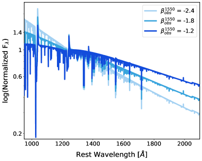
Figure 2: Illustration of the impact of dust attenuation on the observed stellar continuum slope ($\beta_{\rm obs}^{1550}$) keeping a constant underlying stellar population. All three spectra have the same underlying stellar population and are normalized near 1200 Å, but have a varying uniform dust attenuation using the Reddy et al. (2016) law (E(B-V) = 0.05, 0.15, 0.25 for the light blue, blue, and dark blue lines respectively). This leads to three markedly different stellar continuum slopes ($\beta_{\rm obs}^{1550}$$=-2.4,-1.8,-1.2$, respectively).

3.3.2 Properties derived from stellar continuum fit

We derive stellar continuum properties from the best-fit stellar continuum. In particular, we derive the stellar continuum slope ($\beta$), the absolute magnitude ($M_{\rm UV}^{\rm obs}$), $f_{\rm esc,LyC}$, and the ionizing photon production efficiency ($\xi_{\rm ion}$).

The most important property that we measure in this paper is the slope of the FUV stellar continuum at a given wavelength, $\beta^{\lambda}$. We derive the slope between rest-frame 1300 Å and 1800 Å (an average wavelength of 1550 Å) by assuming that

$$F_{\lambda}\propto\lambda^{\beta^{1550}}.$$ (5)

We fit for $\beta^{1550}$ by extrapolating the best-fit stellar continuum model of the LzLCS COS observations described in section 3 to redder wavelengths. We then fit for $\beta_{\rm obs}^{1550}$ assuming a power-law model in the 1300-1800 Å wavelength range of the stellar continuum fit. We tested two other methods to determine $\beta^{1550}$ by using (1) several small wavelength regions in the stellar continuum models without strong stellar or ISM features and (2) fitting for the slope between two points (1300 Å and 1800 Å). We found that all three models produced consistent $\beta^{1550}$ estimates. Since we fit both the stellar population properties (giving the intrinsic continuum slope) and dust attenuation (giving the observed spectral slope), we estimate both the observed continuum slope, $\beta_{\rm obs}^{1550}$, and the intrinsic slope, $\beta_{\rm int}^{1550}$, which is the continuum slope without dust attenuation.

We use $\beta_{\rm obs}^{1550}$ from the stellar continuum modeling instead of the $\beta$ observed in the HST/COS data ($\beta^{\rm COS}$, or $\approx\beta^{\rm 1150}$; Flury et al., 2022a) because it probes the redder wavelengths ($\sim 1550$ Å) that are observed at higher redshift (Finkelstein et al., 2012; Dunlop et al., 2013; Bouwens et al., 2014; Wilkins et al., 2016; Bhatawdekar & Conselice, 2021; Tacchella et al., 2021). The $\beta_{\rm obs}^{1550}$ values scale strongly (Kendall’s rank coefficient of $\tau=0.46$ and p-value of $1\times 10^{-10}$) with $\beta_{\rm COS}$ from Flury et al. (2022a). However, $\beta_{\rm COS}$ values are 14% redder than $\beta_{\rm obs}^{1550}$ measured here, largely because the reddening curve is steeper at bluer wavelengths (see the discussion in section 4) and the intrinsic stellar continuum is slightly flatter between 900-1200 Å than at 1500 Å (Leitherer et al., 1999). Figure 2 shows the same stellar continuum model attenuated by three different E(B-V) values. These three E(B-V) values produce three different $\beta_{\rm obs}^{1550}$ values that bracket the observed LzLCS range. Figure 2 shows unique and distinguishable $\beta^{1150}$ values for the three different E(B-V), but $\beta^{1150}$ is much flatter, especially for high attenuation case, than $\beta^{1550}$. Thus, spectral slopes estimated at 1150 Å are not the same as at 1550 Å. To compare low-redshift observations to high-redshift observations, we must measure $\beta$ at similar wavelengths.

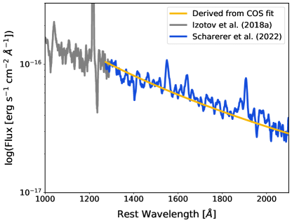
Figure 3: Typical LzLCS data (gray; Izotov et al., 2016a) only probe the blue portion of the spectrum, but recent observations from Schaerer et al. (2022) of J1243+4646 (blue data) compare the extrapolated slope from the LzLCS data (gold line) to the observed continuum slope at 1550 Å. The extrapolated LzLCS continuum slope accurately matches the slope of the redder observations.

How well do the extrapolated fits recover the actual $\beta_{\rm obs}^{1550}$? Recent HST/STIS observations by Schaerer et al. (2022) provide redder observations to test the extrapolated and actual $\beta_{\rm obs}^{1550}$ values. These redder observations are unavailable for the full LzLCS sample, but provide a test of our extrapolation for eight LyC emitters. Figure 3 shows the extrapolated continuum slope from the LzLCS model in gold. The gold line was estimated by fitting the stellar population model to the G140L data between rest-frame wavelengths of 950–1200 Å (gray data). The redder STIS data, shown in dark blue, has a similar slope as the LzLCS fit even though it was not included in the fit ($\beta_{\rm obs}^{1550}$ =-2.56 from the models and -2.50 from the STIS observations). This demonstrates that the extrapolated $\beta_{\rm obs}^{1550}$ matches observed continuum slopes of LzLCS galaxies.

We estimated the observed, or uncorrected for internal extinction, FUV luminosity, L_UV, of the galaxies as the mean flux density of the best-fit stellar model in a 100 Å region centered on 1500 Å. We then converted this into an AB absolute magnitude ($M_{\rm UV}^{\rm obs}$) using the redshift from the SDSS spectra.

Flury et al. (2022a) took the ratio of the observed LyC emission to the fitted stellar continuum to estimate $f_{\rm esc,LyC}$ in a few ways. We predominantly use the $f_{\rm esc,LyC}$ derived from fitting the stellar continuum, but $f_{\rm esc,LyC}$ can also be derived using the observed nebular Balmer emission lines to define the intrinsic LyC emission. The different $f_{\rm esc,LyC}$ estimates scale with each other along a one-to-one relation, although there does exist significant scatter within the relation (see figure 19 in Flury et al., 2022a). Flury et al. (2022a) also derived the relative escape fraction, $f_{\rm esc,LyC}^{\rm rel}$, by comparing the dust-attenuated stellar continuum models to the observed LyC flux. This quantifies the LyC absorption only due to H i within the galaxy.

Finally, we inferred the production efficiency of ionizing photons as

$$\xi_{\rm ion}=\frac{Q}{L_{\rm UV}},$$ (6)

where $Q$ is the intrinsic number of ionizing photons produced by the stellar population and L_UV is the intrinsic mono-chromatic UV luminosity density of the stellar population at 1500 Å. We dereddened the best-fit stellar continuum models, divided each ionizing flux density by the respective photon energy, and integrated over the entire ionizing continuum (21–912Å) to determine $Q$ (although the number of hydrogen ionizing photons is dominated by photons with wavelengths near 912 Å). We then divided $Q$ by the dereddened stellar population flux density at 1500 Å from the models. The LzLCS log($\xi_{\rm ion}$ [s^-1/(erg s^-1 Hz^-1)]) ranges from 24.94 to 25.86 with a median value of 25.47. These $\xi_{\rm ion}$ values bracket the canonical high-redshift value of 25.3 (see section 7), agree with those used in semi-analytical models (Yung et al., 2020), and are similar to the large range of high-redshift $\xi_{\rm ion}$ values (Bouwens et al., 2016; Harikane et al., 2018; Maseda et al., 2020; Stefanon et al., 2022).

4 THE FUV CONTINUUM SLOPE

FUV bright stellar populations are typically characterized by very blue colors because their spectral energy distributions peak in the extreme-ultraviolet (Leitherer et al., 1999; Raiter et al., 2010; Eldridge et al., 2017). The blackbody nature of massive stars leads to a very steep negative power-law index at 1500 Å  with $\beta_{\rm int}^{1550}$ between $-2.8$ and -2.5, after accounting for the nebular continuum, that depends on the age, metallicity, and star formation history of the stellar population (Leitherer et al., 1999). $\beta_{\rm int}^{1550}$ evolves very little over the first 10 Myr after a starburst. This is because 1550 Å is still on the Rayleigh-Jeans portion of the blackbody curve for late O-stars. The non-ionizing FUV light from massive stars propagates out of the galaxy where it is absorbed and attenuated by the same gas and dust that absorbs LyC photons. This dust attenuation flattens the observed spectrum and makes $\beta_{\rm obs}^{1550}$ more positive.

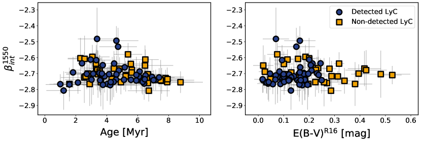
Figure 4: The impact of fitted parameters on the intrinsic slope of the stellar continuum at 1550 Å ($\beta_{\rm int}^{1550}$) for LyC detected (blue circles) and non-detected LyC galaxies (gold squares). Left panel: $\beta_{\rm int}^{1550}$does not scale strongly with the inferred light-weighted ages. Some scatter is introduced due to various stellar evolution that happens between 3-5 Myr. Right Panel: The $\beta_{\rm int}^{1550}$ is uncorrelated with the continuum color excess (E(B-V)^R16).

The stellar population fits allow us to explore the range of $\beta_{\rm int}^{1550}$ within the LzLCS. The $\beta_{\rm int}^{1550}$ has a fairly narrow range of values between -2.8 and -2.5, with a median of -2.71, that does not significantly change with stellar population age (left panel of Figure 4). These values are fully consistent with the narrow range of $\beta_{\rm int}^{1550}$ expected from young stellar populations that include the nebular continuum (Leitherer et al., 1999; Raiter et al., 2010). Figure 4 shows that the $\beta_{\rm int}^{1550}$ spread does not statistically scale with age or E(B-V)^R16 (Kendall’s $\tau$ p-values of 0.062 and 0.37, respectively), and there is also not a statistically-consistent correlation with Z_∗ (p-value of 0.065). When we refer to E(B-V), we denote the attenuation law that we use to emphasize that this value depends on the assumed attenuation law (see Appendix A for how the following results can be recast to any attenuation law). This relatively narrow scatter about a single value arises from $\beta_{\rm int}^{1550}$ depending on the population age, evolutionary sequence, star formation history, and stellar metallicity (in that rough order of importance). The fits to the LzLCS continua suggest that these very young star-forming galaxies occupy a narrow parameter range of age and star-formation history.

The $\beta_{\rm obs}^{1550}$ does not scale significantly with the very young light-weighted stellar population age of the LzLCS (left panel of Figure 5), but scales strongly with the fitted E(B-V)^R16 using a Reddy et al. (2016) attenuation law (right panel of Figure 5). We use linmix, a hierarchical Bayesian linear regression routine that accounts for errors on both variables (Kelly, 2007), to find the relation between E(B-V)^R16 and $\beta_{\rm obs}^{1550}$ is

$$\text{E(B-V)}^{\rm R16}=\left(0.47\pm 0.01\right)+\left(0.171\pm 0.007\right)\times\beta_{\rm obs}^{1550}.$$ (7)

This strong correlation and small scatter suggests that there is a simple analytical relation between E(B-V) and $\beta_{\rm obs}^{1550}$. If we use the assumption that the observed continuum is a power-law with wavelength (Equation 5) and that the observed flux is equal to the intrinsic flux times the dust attenuation factor (Equation 2), we find an analytic relation between E(B-V)  and the continuum slope at the average of two wavelengths ($\lambda^{1}$ and $\lambda^{2}$, respectively) as

$$E(B-V)=\frac{\log_{\rm 10}{\frac{\lambda^{1}}{\lambda^{2}}}}{0.4\Delta k}\left(\beta_{\rm int}^{<1,2>}-\beta_{\rm obs}^{<1,2>}\right),$$ (8)

where $\Delta k$ is the difference in the reddening law at $\lambda^{1}$ and $\lambda^{2}$. This equation emphasizes why it is crucial to compare $\beta_{\rm obs}^{\lambda}$ values at similar wavelengths: if E(B-V) is constant, the estimated $\beta_{\rm obs}^{\lambda}$ depends on the logarithm of the ratio of the two wavelengths used to measure the spectral slope. If we use $\lambda^{1}=1300$ Å and $\lambda^{2}=1800$ Å (the wavelength range used to determine $\beta_{\rm obs}^{1550}$), the $\Delta k$ from the Reddy et al. (2016) law between 1300 and 1800 Å (2.08), and the median $\beta_{\rm int}^{1550}$ of -2.7, we find that E(B-V) is related to the $\beta_{\rm obs}^{1550}$ as

$$E(B-V)^{\rm R16}=0.46+0.17~{}\beta^{\rm 1550}_{\rm obs}.$$ (9)

This agrees with the fitted relationship between E(B-V)^R16 and $\beta_{\rm obs}^{1550}$ (Equation 7). This relation will change based upon the wavelength range that $\beta_{\rm obs}^{1550}$ is determined and the attenuation law that is used (see Appendix A).

Thus, the tight correlation between $\beta_{\rm obs}^{1550}$ and E(B-V) arises due to the shape of the attenuation law and $\beta_{\rm int}^{1550}$. This also explains why there is relatively little scatter within the relationship between E(B-V) and $\beta_{\rm obs}^{1550}$: the extremes of the fitted $\beta_{\rm int}^{1550}$ only change the inferred E(B-V) by 0.1 mags, equivalent to the scatter of E(B-V) at fixed $\beta_{\rm obs}^{1550}$ (Figure 5). Below, we correlate $\beta_{\rm obs}^{1550}$ with parameters like $f_{\rm esc,LyC}$, but Equation 8 stresses that the inferred stellar attenuation, E(B-V), does depend on how well $\beta_{\rm int}^{1550}$ can be constrained. A 0.1 mag scatter is introduced to the E(B-V) observations due to $\beta_{\rm int}^{1550}$. The relatively narrow range of $\beta_{\rm int}^{1550}$ suggests that $\beta_{\rm obs}^{1550}$ is largely set by the dust reddening with a moderate impact from the $\beta_{\rm int}^{1550}$.

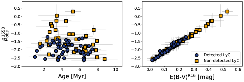
Figure 5: The correlation of the observed continuum slope at 1550Å ($\beta_{\rm obs}^{1550}$) with fitted stellar population parameters for LyC detected (blue circles) and non-detected LyC galaxies (gold squares). Left panel: $\beta_{\rm obs}^{1550}$ does not strongly correlate with the light-weighted age of the stellar population. Right panel: The observed FUV continuum slope strongly correlates with the stellar color excess using Reddy et al. (2016) extinction law, E(B-V)^R16. These two plots strongly suggest that $\beta_{\rm obs}^{1550}$ is largely set by the dust attenuation.

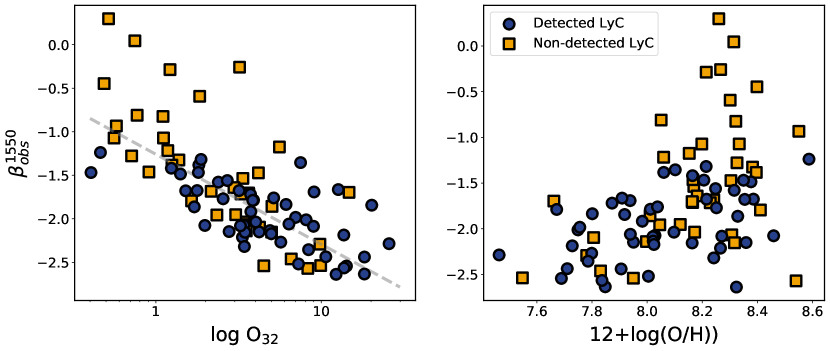
Figure 6: The observed continuum slope at 1550Å ($\beta_{\rm obs}^{1550}$) correlates strongly with galaxy properties derived from the optical spectra for both LyC detected (blue circles) and non-detected galaxies (gold squares). Left panel: $\beta_{\rm obs}^{1550}$ correlates with the flux ratio of the internal attenuation corrected [O iii] 5007 Å and [O ii] 3727 Å flux ratio (O₃₂) at the 5.9$\sigma$ significance. O₃₂ is often used as a proxy of the ionization state of the nebular gas. Galaxies with bluer FUV slopes are more highly ionized. The gray line shows the best-fit relation between $\beta_{\rm obs}^{1550}$ and O₃₂ (Equation 10). Right Panel: The $\beta_{\rm obs}^{1550}$ scales with the oxygen abundance (12+log(O/H)) at the 4.6$\sigma$ significance. The reddest galaxies ($\beta_{\rm obs}^{1550}$ $>-0.75$) do not have direct metallicities and their 12+log(O/H) values are more uncertain. This suggests that more metal rich galaxies have redder continua and that dust attenuation increases with metallicity.

With this analytic understanding of $\beta_{\rm obs}^{1550}$, it is useful to explore how $\beta_{\rm obs}^{1550}$ depends on other observables. The left panel of Figure 6 shows that the internal attenuation corrected O${}_{32}=[\text{O\,{iii}}]\text{5007~{}\AA}/[\text{O\,{ii}}]~{}3727$ Å flux ratio has an inverse, logarithmic, and highly significant (Kendall’s $\tau$ rank coefficient of -0.55, p-value of $2\times 10^{-14}$, or 7.5$\sigma$ significant) trend with $\beta_{\rm obs}^{1550}$. The gray line in Figure 6 shows this best-fit relation of

$$\beta^{1500}_{\rm obs}=\left(-1.3\pm 0.1\right)\times\text{log}_{10}\text{O}_{32}-\left(1.0\pm 0.1\right).$$ (10)

O₃₂ is often quoted as an ionization parameter indicator (Vilchez & Pagel, 1988; Skillman, 1989; McGaugh, 1991; Izotov et al., 2016a), and does not have any direct observational connection to $\beta_{\rm obs}^{1550}$ (although there is a connection to the optical extinction through the Balmer dust correction). Similarly, there is a 6.7$\sigma$ (p-value of 8$\times 10^{-12}$) significant correlation between $\beta_{\rm obs}^{1550}$ and the H$\beta$ equivalent width, another measure of the nebular ionization state.

$\beta_{\rm obs}^{1550}$ also scales with the gas-phase metallicity, 12+log(O/H), with a 4.6$\sigma$ significance (Kendall’s $\tau=0.34$ and p-value of $2\times 10^{-6}$). This trend suggests that $\beta_{\rm obs}^{1550}$ becomes redder for more metal-enriched systems, and that the bluest $\beta_{\rm obs}^{1550}$ values are found in low-metallicity systems. This relation is more scattered than the O₃₂ and EW(H$\beta$) relations, however, all 8 of the galaxies with $\beta_{\rm obs}^{1550}$ greater than -0.75 do not have observations of the temperature sensitive [O iii] 4363 Å line (Flury et al., 2022a). As such, the metallicities of the reddest galaxies may be uncertain by as much as 0.4 dex (Kewley et al., 2006), introducing significant scatter into this relation. Even with this significant calibration uncertainty, there is a nearly 5$\sigma$ trend between $\beta_{\rm obs}^{1550}$ and the gas-phase metallicity.

Finally, we find a 5.9$\sigma$ and 3.4$\sigma$ significant relationship between $\beta_{\rm obs}^{1550}$ and the galaxy stellar mass (M_∗) and observed (uncorrected for dust attenuation) FUV absolute magnitude ($M_{\rm UV}^{\rm obs}$), respectively. These relations suggest that lower mass and fainter galaxies have bluer stellar continuum slopes. We fully introduce and discuss the importance of these relations in section 7.

In this section we have explored relationships between both $\beta_{\rm int}^{1550}$ and $\beta_{\rm obs}^{1550}$. We found that $\beta_{\rm int}^{1550}$ has a narrow range of values, but does not scale significantly with other properties. We found significant correlations between $\beta_{\rm obs}^{1550}$ and the fitted E(B-V)^R16, the observed optical [O iii]/[O ii] flux ratio, the H$\beta$ equivalent width, M_∗, $M_{\rm UV}^{\rm obs}$, and the gas-phase 12+log(O/H). With these correlations in mind, the next section explores the correlation between $\beta_{\rm obs}^{1550}$ and the LyC escape fraction.

5 PREDICTING THE LYMAN CONTINUUM ESCAPE FRACTION WITH $\beta$

The previous section found that $\beta_{\rm obs}^{1550}$ scales strongly with the continuum color excess, E(B-V). Similarly, Saldana-Lopez et al. (2022) found a strong correlation between E(B-V) and $f_{\rm esc,LyC}$. Thus, Figure 5 suggests that $\beta_{\rm obs}^{1550}$ likely correlates with $f_{\rm esc,LyC}$ (Flury et al., 2022b). Figure 7 shows the relationship between $f_{\rm esc,LyC}$ and $\beta_{\rm obs}^{1550}$ with the LyC detected sample as circles and the non-detected LyC galaxies as downward pointing arrows at their corresponding 1$\sigma$ $f_{\rm esc,LyC}$ upper-limits.

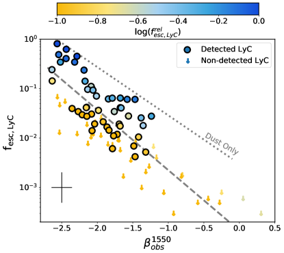
Figure 7: The LyC escape fraction ($f_{\rm esc,LyC}$) strongly scales with the observed stellar continuum slope at 1550 Å ($\beta_{\rm obs}^{1550}$). The LyC detections are shown as circles and the non-detections as downward pointing arrows. Representative error bars for the LyC detections are shown in the bottom left corner. Both detections and non-detections are color coded by their relative escape fractions ($f_{\rm esc,LyC}^{\rm rel}$), or the fraction of ionizing photons absorbed only by neutral hydrogen. At fixed $\beta_{\rm obs}^{1550}$ there is a strong vertical gradient in the color of the plotted points, suggesting that neutral hydrogen introduces significant scatter at fixed dust properties. The gray dashed line shows the best-fit relation for $f_{\rm esc,LyC}$ in terms of $\beta_{\rm obs}^{1550}$ (Equation 11) which accounts for both the $f_{\rm esc,LyC}$ non-detections and the errors on both $\beta_{\rm obs}^{1550}$ and $f_{\rm esc,LyC}$. The gray dotted line shows the theoretical relation assuming that only dust attenuation removes ionizing photons (Equation 16). This acts as an upper envelope for the observations.

$\beta_{\rm obs}^{1550}$ scales strongly with $f_{\rm esc,LyC}$. The median $\beta_{\rm obs}^{1550}$ of the LyC detected sample is -2.00 and -1.63 for the non-detected sample, indicating that LyC emitting galaxies have substantially bluer continuum slopes. Using a Kendall’s $\tau$ test for censored data (the $R$ package cenken), we find that the $\beta_{\rm obs}^{1550}$ scales with $f_{\rm esc,LyC}$ at the 5.7$\sigma$ significance (Kendall’s $\tau=-0.42$ and a p-value of $5\times 10^{-9}$). We use linmix (Kelly, 2007), a hierarchical Bayesian linear regression routine which accounts for the errors on both $f_{\rm esc,LyC}$ and $\beta_{\rm obs}^{1550}$ as well as for the upper limits on $f_{\rm esc,LyC}$, to find the analytic relation between $f_{\rm esc,LyC}$ and $\beta_{\rm obs}^{1550}$ (the gray dashed line on Figure 7) of

$$f_{\rm esc,LyC}=\left(1.3\pm 0.6\right)\times 10^{-4}\times 10^{\left(-1.22\pm 0.1\right)\beta^{1550}_{\rm obs}}.$$ (11)

Many theoretical models for reionization suggest that star-forming galaxies must emit more than 5, 10, or 20% of their ionizing photons to reionize the IGM (Ouchi et al., 2009; Robertson et al., 2013; Robertson et al., 2015; Rosdahl et al., 2018; Finkelstein et al., 2015, 2019; Naidu et al., 2020). Equation 11 suggests that these $f_{\rm esc,LyC}$ occur on average in the LzLCS for $\beta_{\rm obs}^{1550}$ values less than $-2.11$, $-2.35$, and $-2.60$, respectively. We also find a 2.9 and 3.4$\sigma$ significant correlation (p-values of 0.002 and 0.0003, respectively) between $\beta_{\rm obs}^{1550}$ and $f_{\rm esc,LyC}^{\rm rel}$ and the escape fraction calculated using the H$\beta$ equivalent width (Flury et al., 2022a). Thus, $\beta_{\rm obs}^{1550}$ correlates with complementary $f_{\rm esc,LyC}$ measures.

Equation 11 describes the population average relation between $\beta_{\rm obs}^{1550}$ and $f_{\rm esc,LyC}$. This relation contains real and significant scatter that must be addressed when applying it to higher redshift observations. With the appreciable scatter in this relation, Equation 11 more robustly estimates population averaged escape fractions rather than individual galaxy-by-galaxy escape fractions. How much of the scatter is physical? The LzLCS $f_{\rm esc,LyC}$ detections have a median signal-to-noise of 3 (Flury et al., 2022a). Thus, there are significant observational uncertainties in the $f_{\rm esc,LyC}$ measurements (see the representative error bars in the lower left of Figure 7). linmix estimates that about 0.15 dex of the scatter in Figure 7 is intrinsic to the relationship. A possible source of intrinsic scatter is the neutral gas column density, the neutral gas covering fraction, or the geometry. These have been observed to scale strongly with $f_{\rm esc,LyC}$ in the LzLCS (Saldana-Lopez et al., 2022). The points in Figure 7 are color-coded by $f_{\rm esc,LyC}^{\rm rel}$ or the escape fraction in the absence of dust. While $f_{\rm esc,LyC}^{\rm rel}$ only moderately scales with $\beta_{\rm obs}^{1550}$ (3.4$\sigma$), at fixed $\beta_{\rm obs}^{1550}$ there is a strong vertical $f_{\rm esc,LyC}^{\rm rel}$ gradient, which may suggest that galaxy-to-galaxy variations in neutral gas sets the scatter in Figure 7. This strong secondary scaling with $f_{\rm esc,LyC}^{\rm rel}$ echoes the findings in section 4 where $\beta_{\rm obs}^{1550}$ strongly scales with O₃₂ and H$\beta$ EW, both which trace the ionization state. In a future paper (Jaskot et al. in preparation), we will explore multivariate correlations with $f_{\rm esc,LyC}$ and $\beta_{\rm obs}^{1550}$, O₃₂, H$\beta$ equivalent width, metallicity, or star formation rate surface density.

Finally, Figure 8 shows the scaling relation between $\beta_{\rm obs}^{1550}$ and the emitted ionizing efficiency ($\xi_{\rm ion}\times f_{\rm esc}$). Using linmix we determine this relation to be

$$\xi_{\rm ion}\times f_{\rm esc}=(4\pm 2)\times 10^{21}\text{[s${}^{-1}$ / erg s${}^{-1}$ Hz${}^{-1}$]}\times 10^{\left(-1.2\pm 0.1\right)\text{$\beta_{\rm obs}^{1550}$}}.$$ (12)

This has a similar $\beta_{\rm obs}^{1550}$ dependence as the $f_{\rm esc,LyC}$ relation given in Equation 11 with a power law exponent of -1.2. The scatter on the emitted ionizing efficiency relation is similar to the scatter in Equation 11, consistent with the insignificant relationship found between $\beta_{\rm obs}^{1550}$ and $\xi_{\rm ion}$ (p-value of 0.155). Thus, the ionizing emissivity scales the relation between $\beta_{\rm obs}^{1550}$ and $f_{\rm esc,LyC}$ to include the production efficiency of ionizing photons. In section 7 we use Equation 12 to estimate the ionizing emissivity of galaxies during the epoch of reionization.

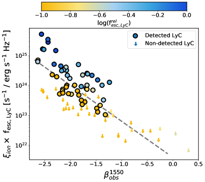
Figure 8: The LyC escape fraction ($f_{\rm esc,LyC}$) times the ionizing photon production efficiency ($\xi_{\rm ion}$ = Q/L_UV) strongly correlates with the observed continuum slope at 1550 Å ($\beta_{\rm obs}^{1550}$). The gray dashed line shows the best-fit relation for $f_{\rm esc,LyC}$ $\times$ $\xi_{\rm ion}$ in terms of $\beta_{\rm obs}^{1550}$ (Equation 12) that accounts for both the $f_{\rm esc,LyC}$ upper-limits and errors.

6 IMPLICATIONS FOR THE ESCAPE OF IONIZING PHOTONS

The FUV spectral slope strongly correlates with $f_{\rm esc,LyC}$. Figure 4 and Figure 5 demonstrate that the major determinant of the FUV spectral slope is the dust attenuation derived from the observed continuum shape. Dust connects the gas-phase metallicity through the dust-to-gas ratio, and to the ionization state of the gas because metals are the predominate nebular coolant. The metallicity of the gas strongly depends on the stellar mass of the galaxies through the mass-metallicity relation (Tremonti et al., 2004; Berg et al., 2012) and the mass-luminosity relation. Therefore, $\beta_{\rm obs}^{1550}$, M_∗, O₃₂, $M_{\rm UV}^{\rm obs}$, and E(B-V) are all linked together through the gas-phase metallicity. It is not entirely surprising then that section 4 found that all of these parameters correlate. This connection between LyC and dust echoes relations between Ly$\alpha$ and dust (Hayes et al., 2011). Here we explore the physical connection between $\beta_{\rm obs}^{1550}$ and $f_{\rm esc,LyC}$ and how the observed $\beta_{\rm obs}^{1550}$-$f_{\rm esc,LyC}$ relation informs on how ionizing photons escape galaxies.

To explore the connection between $\beta_{\rm obs}^{1550}$ and $f_{\rm esc,LyC}$, we revisit the absolute escape fraction definition (see Saldana-Lopez et al., 2022). There are two main sinks of ionizing photons: dust (with an optical depth of $\tau_{\rm dust}$) and H i (Chisholm et al., 2018). Thus, $f_{\rm esc,LyC}$ is determined as the product of the attenuation of dust and $f_{\rm esc,LyC}^{\rm rel}$ as

$$f_{\rm esc,LyC}=10^{-0.4\tau_{\rm dust}}\times f_{\rm esc,LyC}^{\rm rel}~{},$$ (13)

where

$$\tau_{\rm dust}(912)=k(912)~{}{\rm E(B-V)}.$$ (14)

A possible explanation for the significant correlation between $\beta_{\rm obs}^{1550}$ and $f_{\rm esc,LyC}$ is that dust is the only sink of ionizing photons. This can be tested by assuming that the H i transmits all of the ionizing photons ($f_{\rm esc,LyC}^{\rm rel}$ = 1). Equation 13 then only depends on the dust as

$$\log(f_{\rm esc,LyC}^{\rm dust})\approx-0.4\tau_{\rm dust}(912)=-0.4E(B-V)k(912).$$ (15)

Using Equation 8, Equation 9, and the fact that k(912)=12.87 for the Reddy et al. (2016) extinction law, this equation can be redefined in terms of $\beta_{\rm obs}^{1550}$ as

$$\log(f_{\rm esc,LyC}^{\rm dust})\approx-k(912)\frac{\log_{\rm 10}{\frac{\lambda^{1}}{\lambda^{2}}}}{\Delta k}\left(\beta_{\rm int}-\beta_{\rm obs}\right)=-2.4-0.9\beta^{1550}_{\rm obs}.$$ (16)

We overplot this relation as the dotted line in Figure 7 and see that this relation provides a strong upper envelope for $f_{\rm esc,LyC}$. There are no observed points above this “dust only” line. All the points lie below the “dust only” line because neutral gas also decreases $f_{\rm esc,LyC}$. As emphasized in Equation 13, $f_{\rm esc,LyC}$ is the product of the dust and $f_{\rm esc,LyC}^{\rm rel}$. This naturally explains why there is a strong gradient of $f_{\rm esc,LyC}^{\rm rel}$ in Figure 7 at fixed $\beta_{\rm obs}^{1550}$: the absolute escape fraction is a product of both dust and H i opacity. Saldana-Lopez et al. (2022) used the Lyman Series absorption lines to find that the points close to the “dust only” line have very low neutral gas covering fractions and H i absorbs little LyC, explaining why $f_{\rm esc,LyC}^{\rm rel}$ $\sim 100$% for these points.

7 IMPLICATIONS FOR COSMIC REIONIZATION

The goal of the LzLCS is to provide local examples of LyC escape that are directly transferable to high-redshift observations to determine their contribution to reionization. To reionize the early IGM, star-forming galaxies must have an ionizing emissivity, $\dot{n}_{\rm ion}$, much larger than the cosmic baryon density at high-redshift. Equation 1 infers $\dot{n}_{\rm ion}$ if the integrated FUV luminosity function ($\rho_{\rm UV}$), the ionizing efficiency ($\xi_{\rm ion})$, and $f_{\rm esc,LyC}$ are observed (Ouchi et al., 2009; Robertson et al., 2013; Robertson et al., 2015; Finkelstein et al., 2015, 2019; Mason et al., 2019; Naidu et al., 2020). Above, we have provided an empirical route to estimate $f_{\rm esc,LyC}$ and $\xi_{\rm ion}$$\times$$f_{\rm esc,LyC}$ using the FUV continuum slope, a common observable of high-redshift galaxies (Finkelstein et al., 2012; Dunlop et al., 2013; Bouwens et al., 2014; Wilkins et al., 2016; Roberts-Borsani et al., 2021; Bhatawdekar & Conselice, 2021; Tacchella et al., 2021). If we assume that these LzLCS relations apply to high-redshift galaxies, do early star-forming galaxies emit sufficient ionizing photons to reionize the early IGM?

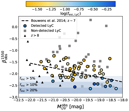
Figure 9: The observed absolute FUV magnitude ($M_{\rm UV}^{\rm obs}$) of the LyC detections (colored circles) and non-detections (gray squares) for the LzLCS sample scales with the observed stellar continuum slope at 1550 Å ($\beta_{\rm obs}^{1550}$) at the 3.4$\sigma$ significance. Brighter LzLCS galaxies are redder and possibly emit a smaller fraction of their ionizing photons. The $\beta_{\rm obs}^{1550}$-$M_{\rm UV}^{\rm obs}$ observed at $z\sim 7$ from Bouwens et al. (2014) is included as a dashed line. This $z\sim 7$ relation matches the general trend of the LyC detections in the LzLCS. Black triangles show individual $z>8$ galaxies from Wilkins et al. (2016), Bhatawdekar & Conselice (2021), and Tacchella et al. (2021). The LyC detections are colored by the observed LyC escape fraction (log($f_{\rm esc,LyC}$)) to emphasize galaxies with $f_{\rm esc,LyC}$ $>$5% as blue points. We use Equation 11 and $\beta_{\rm obs}^{1550}$ to estimate population averages of $f_{\rm esc,LyC}$ equal to 5, 10, and 20% . In general, fainter galaxies have larger $f_{\rm esc,LyC}$.

Figure 9 compares $\beta_{\rm obs}^{1550}$ to the LzLCS observed (not corrected for dust) $M_{\rm UV}^{\rm obs}$. We color-code the LzLCS points as gray squares for non-detections and detected galaxies with the observed $f_{\rm esc,LyC}$. The colorbar is shifted such that blue points represent so called “cosmologically relevant” escape fractions ($>$5%). Using the relationship between $\beta_{\rm obs}^{1550}$ and $f_{\rm esc,LyC}$ (Equation 11) we shade regions of this figure that correspond to LzLCS population averages of 5, 10, and 20% escape fractions. This shading emphasizes that the LzLCS galaxies with $f_{\rm esc,LyC}$ greater than 5% are predominately found at fainter $M_{\rm UV}^{\rm obs}$ (Flury et al., 2022b).

Many previous studies have explored the median relationship between $\beta_{\rm obs}^{1550}$ and $M_{\rm UV}^{\rm obs}$ at high-redshift (Finkelstein et al., 2012; Dunlop et al., 2013; Bouwens et al., 2014). Bouwens et al. (2014) fit the $\beta_{\rm obs}^{1550}$-$M_{\rm UV}^{\rm obs}$ relation at different redshifts as

$$\beta^{1550}_{\rm obs}=b+a(M_{\rm UV}^{\rm obs}+19.5).$$ (17)

Table 3 in Bouwens et al. (2014) gives the $a$ and $b$ values for six different redshifts from 2.8 – 8. We note that the $z=8$ $\beta_{\rm obs}^{1550}$-$M_{\rm UV}^{\rm obs}$ relation from Bouwens et al. (2014) has a fixed slope ($a$ value) due to the uncertain $Y$-band data. The dashed line in Figure 9 shows the $z=7$ relation over the LzLCS observations. The high-redshift relation matches the LzLCS across most $M_{\rm UV}^{\rm obs}$. This suggests that the LzLCS and $z\sim 7$ galaxies have a similar relation between their FUV brightnesses and continuum slopes. Combining the observed $z\sim 7$ $\beta_{\rm obs}^{1550}$-$M_{\rm UV}^{\rm obs}$ relation (Equation 17) and the LzLCS $\beta_{\rm obs}^{1550}$-$f_{\rm esc,LyC}$ relation (Equation 11), we predict the population-averaged $f_{\rm esc,LyC}$ at various redshifts as

$$f_{\rm esc,LyC}=1.3\times 10^{-4}\times 10^{-1.22\left(b+a\left[M_{\rm UV}^{\rm obs}+19.5\right]\right)}.$$ (18)

In Figure 10, we overplot this predicted $z\sim 7$ relationship using the $a$ and $b$ values from Bouwens et al. (2014) as a light blue line. The dashed gray line illustrates the best-fit LzLCS relation using linmix (Kelly, 2007) to account for the $f_{\rm esc,LyC}$ upper limits and the errors on both $f_{\rm esc,LyC}$ and $M_{\rm UV}^{\rm obs}$. The LzLCS and $z\sim 7$ relations have relatively large error bars, but their slopes and normalizations are statistically similar (a slope in log-space of $0.34\pm 0.10$ and $0.25\pm 0.09$ for the LzLCS and $z\sim 7$ relations, respectively). Thus, the $z\sim 7$ relation roughly reproduces the observed LzLCS trend. The observed log-space trend is very shallow (Flury et al., 2022b) and suggests only a factor of 10 $f_{\rm esc,LyC}$ change in over 4 orders of magnitude of $M_{\rm UV}^{\rm obs}$. The large LzLCS $M_{\rm UV}^{\rm obs}$ dynamic range likely explains why smaller previous samples did not find a statistically significant trend between $M_{\rm UV}^{\rm obs}$ and $f_{\rm esc,LyC}$ (Izotov et al., 2021).

Using the Bouwens et al. (2014) observations, Equation 18 predicts that $z\sim 7$ galaxies emit $>5$% ($>20$%) of their ionizing photons if they are fainter than $M_{\rm UV}^{\rm obs}$ $>$ -19.2 mag ($-16.7$ mag; see the shading in Figure 9). Other works have made similar $\beta_{\rm obs}^{1550}$ observations at high-redshift. Dunlop et al. (2013) find $\beta_{\rm obs}^{1550}$ = $-2.08$ at $z\sim 7$ for $M_{\rm UV}^{\rm obs}$ = $-18.5$ mag galaxies and $-1.81$ for $M_{\rm UV}^{\rm obs}$ = $-19.5$ mag galaxies. This leads to a population average $f_{\rm esc,LyC}$ $\simeq$ 5% for faint galaxies, while brighter galaxies have an $f_{\rm esc,LyC}$ of 2%. The triangles in Figure 9 show individual $z>8$ galaxies (Wilkins et al., 2016; Bhatawdekar & Conselice, 2021; Tacchella et al., 2021). While sparsely sampled at the moment, $z>8$ galaxies fainter than $-20.5$ mag have a median $\beta_{\rm obs}^{1550}$ = $-2.1$ (suggesting an $f_{\rm esc,LyC}$ near 5%) and galaxies brighter than $-20.5$ have $\beta_{\rm obs}^{1550}$ = $-1.9$. Since $\beta_{\rm obs}^{1550}$ largely tracks the dust contribution to $f_{\rm esc,LyC}$ (section 6), we can use Equation 16 to put an upper limit of $f_{\rm esc,LyC}$ $<30$% for the individual $M_{\rm UV}^{\rm obs}$ $>$ $-20.5$ $z\sim 8$ galaxies. This is the “dust free” scenario and modest $f_{\rm esc,LyC}^{\rm rel}$ can reduce $f_{\rm esc,LyC}$ to population averages of 5%. Finally, we note that the LzLCS $\beta_{\rm obs}^{1550}$-$M_{\rm UV}^{\rm obs}$ relations are entirely consistent with semi-analytical models of $\beta_{\rm obs}^{1550}$ at high-redshift, including the large scatter to higher $\beta_{\rm obs}^{1550}$ values (Yung et al., 2019).

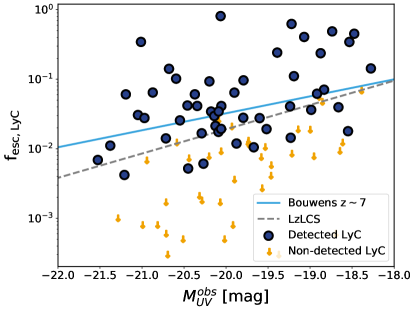
Figure 10: The observed absolute FUV magnitude ($M_{\rm UV}^{\rm obs}$) versus the observed LyC escape fraction ($f_{\rm esc,LyC}$) for galaxies with detected (blue circles) and non-detected (downward pointing arrows) LyC emission. The inferred relationship at $z\sim 7$ is shown as a light blue line using Equation 18 and the observed relation between $\beta_{\rm obs}^{1550}$ and $M_{\rm UV}^{\rm obs}$  from Bouwens et al. (2014). The best-fit relation from the LzLCS, accounting for the upper limits on $f_{\rm esc,LyC}$, is shown as the dashed gray line. The LzLCS and $z\sim 7$ relations have statistically similar slopes ($0.34\pm 0.10$ and $0.25\pm 0.09$ for the LzLCS and $z\sim 7$ relation, respectively) and normalizations ($5.27\pm 2.1$ and $5.14\pm 0.3$ respectively).

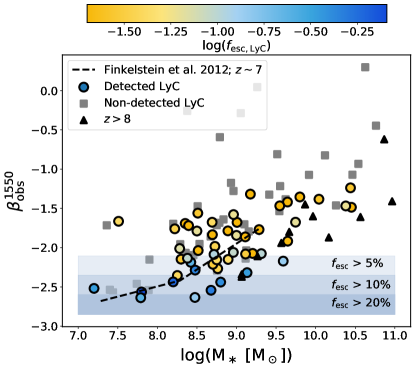
Figure 11: LzLCS galaxies that are blue and low stellar mass (M_∗) tend to have larger LyC escape fractions. The $\beta_{\rm obs}^{1550}$ of the LzLCs detections (colored circles) and non-detections (gray squares) scale with the M_∗ at the 5.9$\sigma$ significance. We include the $z\sim 7$ relation from Finkelstein et al. (2012) as the dashed line and individual $z>8$ galaxies from Wilkins et al. (2016), Bhatawdekar & Conselice (2021), and Tacchella et al. (2021) as black triangles. The LzLCS LyC detections are colored by the observed LyC escape fraction (log($f_{\rm esc,LyC}$)), such that galaxies with $f_{\rm esc,LyC}$ $>$ 5% are blue. We use Equation 11 to shade regions of the plot that correspond to 5, 10, and 20% $f_{\rm esc,LyC}$. The overall trend suggested by the LzLCS for the high-redshift galaxies is that lower M_∗ galaxies have higher $f_{\rm esc,LyC}$.

The stellar mass, M_∗, represents the integrated star formation of a given galaxy. Figure 11 shows the 5.9$\sigma$ significant relationship between M_∗ and $\beta_{\rm obs}^{1550}$. More massive galaxies have redder continuum slopes than their lower mass counterparts, likely as their gas-phase metallicity (Tremonti et al., 2004; Mannucci et al., 2010; Berg et al., 2012) and dust content increases (Rémy-Ruyer et al., 2013; Popping et al., 2017; Popping & Péroux, 2022). The relationship between $\beta_{\rm obs}^{1550}$ and M_∗ for a sample of $z\sim 7$ galaxies from Finkelstein et al. (2012) is overplotted as a black dashed line in Figure 11. We choose the $z\sim 7$ range from Finkelstein et al. (2012) because $z\sim 7$ is squarely within the epoch of reionization and it is the same redshift used for $M_{\rm UV}^{\rm obs}$ from Bouwens et al. (2014). Similar to Figure 9, the correspondence between the high redshift samples and the LzLCS is striking: the Finkelstein et al. (2012) relation tracks through the center of the LzLCS points (both detections and non-detections). This suggests that the LzLCS $\beta_{\rm obs}^{1550}$ varies with host galaxy properties in similar ways as high-redshift galaxies. We use Equation 11 to shade regions in Figure 11 of expected $f_{\rm esc,LyC}$ values. On average, $z\sim 7$ galaxies with logM_∗$<8.7$ (7.6) emit more than 5% (20%) of their ionizing photons. Figure 11 also includes individual $z>8$ galaxies from the literature (Wilkins et al., 2016; Bhatawdekar & Conselice, 2021; Tacchella et al., 2021). Of all the individual $z>8$ galaxies, only GOODSN-35589 and EGS-68560, both at logM_∗ = 9.1, are blue enough to emit more than 5% of their ionizing photons. These galaxies are weak LyC emitters with a predicted $f_{\rm esc,LyC}$ $\sim$ 6%. The other $z>8$ sources are too red to emit appreciable LyC. This is likely because most of the individual literature sources are biased towards bright and massive galaxies. If the LzLCS relationship between $\beta_{\rm obs}^{1550}$ and $f_{\rm esc,LyC}$ holds for galaxies within the epoch of reionization, faint and low stellar mass galaxies likely dominate the ionizing photon budget.

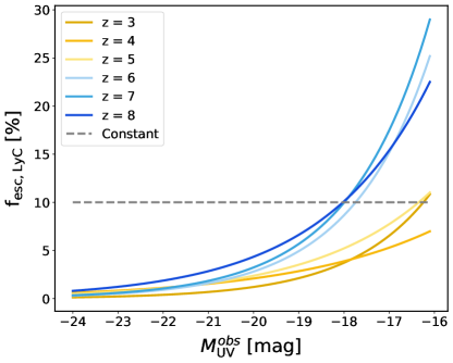
Figure 12: The inferred evolution of $f_{\rm esc,LyC}$ at high-redshift, assuming the relation between $\beta_{\rm obs}^{1550}$ and $f_{\rm esc,LyC}$ (Figure 7) applies for the $M_{\rm UV}^{\rm obs}$-$\beta_{\rm obs}^{1550}$ relations from Bouwens et al. (2014) (Equation 17). We estimate $f_{\rm esc,LyC}$ at 6 different redshifts and provide an estimate of the evolution of $f_{\rm esc,LyC}$ with $M_{\rm UV}^{\rm obs}$. The $f_{\rm esc,LyC}$ varies shallowly with $M_{\rm UV}^{\rm obs}$ for galaxies brighter than $-20$ mag. In general, these observationally-motivated relations suggest that fainter galaxies at higher redshifts emit a larger fraction of their ionizing photons.

The LzLCS relations and the high-redshift $\beta_{\rm obs}^{1550}$ observations allow for some of the first indirect estimates of $f_{\rm esc,LyC}$ during the epoch of reionization. We convert the Bouwens et al. (2014) $\beta_{\rm obs}^{1550}$ relations in Equation 18 into population averages of $f_{\rm esc,LyC}$ using the LzLCS relation. The predicted $f_{\rm esc,LyC}$ curves for $M_{\rm UV}^{\rm obs}$ down to -16 mag, often the current detection limits, are plotted in Figure 12 for 6 different redshifts. These observationally motivated relations suggest that only galaxies fainter than -16 mag have $f_{\rm esc,LyC}$ $>$10% at $z<5$. This is broadly consistent with current samples of LyC emitters at $z\sim 3$: galaxies brighter than L${}^{\ast}_{z=3}$ ($M_{\rm UV}^{\rm obs}$ = -21 mag) have non-detected LyC, while $f_{\rm esc,LyC}$ increases with decreasing luminosity and is $f_{\rm esc,LyC}$ $\sim$ 12% for galaxies fainter than L${}^{\ast}_{z=3}$ (Pahl et al., 2021). During the epoch of reionization (blue curves), all galaxies brighter than L${}^{\ast}_{z=3}$ ($M_{\rm UV}^{\rm obs}$ $\lesssim-21$ mag) have population-averaged escape fractions less than 5%. $f_{\rm esc,LyC}$ increases for fainter galaxies as their $\beta_{\rm obs}^{1550}$ becomes bluer. During the epoch of reionization, the population averaged $f_{\rm esc,LyC}$ exceeds 10% for $M_{\rm UV}^{\rm obs}$ values fainter than -18 mag. These $f_{\rm esc,LyC}$ trends are in slight tension with recent $f_{\rm esc,LyC}$ estimates using the Ly$\alpha$ luminosity function (Matthee et al., 2022). This work found the $z\sim 7$ $f_{\rm esc,LyC}$ distribution to peak near $f_{\rm esc,LyC}$ = 11% for galaxies with $M_{\rm UV}^{\rm obs}$ = -19.5 (a value two times higher than predicted in Figure 12) and decreases for both brighter and fainter galaxies. The difference could be due to a $\beta_{\rm obs}^{1550}$ tracing the evolving metal content of galaxies while Matthee et al. (2022) determine $f_{\rm esc,LyC}$ from the Ly$\alpha$ properties.

Can metallicity evolution explain the dramatic increase of $f_{\rm esc,LyC}$ from $z=5$ to $z=6$ observed in Figure 12 as reionization concludes? The increase in $f_{\rm esc,LyC}$ at $z>6$ for faint galaxies in Figure 12 is due to the $b$ value in Equation 17 from Bouwens et al. (2014) becoming more negative. The $b$ measures the $\beta_{\rm obs}^{1550}$ zero-point at fixed $M_{\rm UV}^{\rm obs}$. As $b$ becomes more negative, from $-1.9\pm 0.02$ at $z=5$ to $-2.13\pm 0.44$ at $z=8$, galaxies become bluer at fixed $M_{\rm UV}^{\rm obs}$. What causes this blue shift? Figure 6 and Figure 11 show that changes to gas-phase ionization, metallicity, and M_∗ heavily impacts $\beta_{\rm obs}^{1550}$. Galaxies that vigorously form stars (and simultaneously produce ionizing photons), also rapidly synthesize metals. As galaxies grow in M_∗ they retain more of the these metals (Tremonti et al., 2004), allowing for them to create more dust (Rémy-Ruyer et al., 2013; Popping et al., 2017; Popping & Péroux, 2022). Thus, the rapid buildup of stellar mass and metallicity during the epoch of reionization could lead to redder $\beta_{\rm obs}^{1550}$ and push $f_{\rm esc,LyC}$ to lower values at later times.

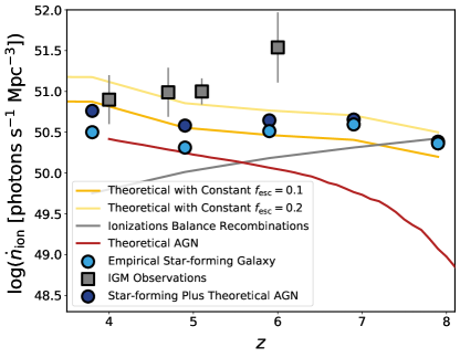
Figure 13: An observationally-motivated estimate of the ionizing emissivity ($\dot{n}_{\rm ion}$) during the epoch of reionization. The light blue circles are the values predicted using the LzLCS relation between $\beta_{\rm obs}^{1550}$ and $\xi_{\rm ion}$$\times$$f_{\rm esc,LyC}$ (Equation 12) and the observed $M_{\rm UV}^{\rm obs}$-$\beta_{\rm obs}^{1550}$ relation (Equation 17) at redshifts 4, 5, 6, 7, and 8 from Bouwens et al. (2014). The dark and light gold curves are estimates assuming a constant $f_{\rm esc,LyC}$ of 10 and 20%, respectively. The gray squares are observations of the ionizing emissivity (Becker & Bolton, 2013; Becker et al., 2021). The gray line is the ionizing emissivity required for ionization to balance recombination at a given redshift (Madau et al., 1999; Ouchi et al., 2009), assuming a redshift-dependent clumping factor (Shull et al., 2012). Values above the gray line will increase the hydrogen ionization fraction in the IGM. The red line is a theoretical estimate of the AGN emissivity from Finkelstein et al. (2019). The dark blue circles are the sum of the AGN and the empirical star-forming ionizing emissivities. Star-forming galaxies dominate the ionizing emissivity at $z>5$. The observationally-motivated $\dot{n}_{\rm ion}$ is statistically consistent with the observed redshift 4 and 5 points, in marginal statistical tension with the $z\sim 6$ data point, and suggests that star-forming galaxies began to emit sufficient ionizing photons to shift the IGM ionization state near redshifts of 8.

The LzLCS $\beta_{\rm obs}^{1550}$-$f_{\rm esc,LyC}$ relationship and the empirical scaling between $\beta_{\rm obs}^{1550}$ and $M_{\rm UV}^{\rm obs}$ can estimate $\dot{n}_{\rm ion}$ at high-redshift. We use the luminosity function from Bouwens et al. (2015) and integrate from -24 to -16 mag (or approximately 0.01L^∗) for $z=$4, 5, 6, 7, and 8 respectively. We use the luminosity functions from Bouwens et al. (2015) largely for consistency with the observed $M_{\rm UV}^{\rm obs}$-$\beta_{\rm obs}^{1550}$ relations (Equation 17), but other luminosity functions provide similar results at these $M_{\rm UV}^{\rm obs}$ values (Livermore et al., 2017; Atek et al., 2018).

First, we follow previous work and assume a constant log($\xi_{\rm ion})=25.27$ (Bouwens et al., 2016) measured for a population of galaxies at $z\sim 4-5$. This $\xi_{\rm ion}$ is broadly consistent with values used in theoretical studies (Robertson et al., 2013; Robertson et al., 2015; Naidu et al., 2020). In this base case, we assume a constant $f_{\rm esc,LyC}$ for all galaxies of 10% (dark gold line in Figure 13) and 20% (light gold line in Figure 13), again similar to previous work (Robertson et al., 2013; Robertson et al., 2015). The gray line in Figure 13 estimates the $\dot{n}_{\rm ion}$ needed to balance hydrogen ionization and recombinations in the IGM at a given redshift (Madau et al., 1999; Ouchi et al., 2009), assuming a clumping factor that evolves with redshift (Shull et al., 2012). If $\dot{n}_{\rm ion}$ is greater than the gray line, ionizations occur more frequently than recombinations and the ionization state of the IGM increases. When $\dot{n}_{\rm ion}$ is less than this gray line, recombinations occur more frequently than photoionizations, and the ionization state of the IGM becomes more neutral (or does not change if the IGM is already neutral). Future work will refine these prescriptions and use semi-analytic models to solve the differential equations required to quantify the impact of the LzLCS prescriptions on the IGM reionization history (Trebitsch in preparation).

The gold lines roughly intersect with the gray line between $z\sim 7-8$. This suggests that star-forming galaxies with constant properties produce enough ionizing photons to increase the IGM ionization fraction near redshifts of 8 (Ouchi et al., 2009; Robertson et al., 2013; Robertson et al., 2015). The ionizing emissivity of star-forming galaxies continues to rise at lower redshifts as the number density of galaxies increases.

The LzLCS and high-redshift data suggest that $f_{\rm esc,LyC}$ is not constant, but rather varies with $\beta_{\rm obs}^{1550}$, M_∗, and $M_{\rm UV}^{\rm obs}$. Does the LzLCS $\beta_{\rm obs}^{1550}$-$f_{\rm esc,LyC}$ relation and high-redshift $\beta_{\rm obs}^{1550}$  observations suggest a similar production of ionizing photons as these constant assumptions? Using the Bouwens et al. (2014) $\beta_{\rm obs}^{1550}$-$M_{\rm UV}^{\rm obs}$ relations (Equation 17), we test two LzLCS relations: (1) the LzLCS $\beta_{\rm obs}^{1550}$-$f_{\rm esc,LyC}$ (Equation 18) with a constant log($\xi_{\rm ion}$) = 25.27 and (2) the LzLCS $\beta_{\rm obs}^{1550}$-$\xi_{\rm ion}$$\times$$f_{\rm esc,LyC}$ relation (Equation 12). We integrate the product of these relations and the luminosity functions from -23 to -16 mag. These two predicted $\dot{n}_{\rm ion}$ values track each other within 0.2 dex (the constant $\xi_{\rm ion}$ has lower $\dot{n}_{\rm ion}$), and we only include the relation using $\xi_{\rm ion}$$\times$$f_{\rm esc,LyC}$ in Figure 13 for clarity (the light blue points in Figure 13).

The empirically-motivated $\dot{n}_{\rm ion}$ values exceeds the value to balance recombinations between $z\sim 7-8$. Near these redshifts, star-forming galaxies produce sufficient ionizing photons to increase the IGM ionization fraction. While we currently do not have statistical populations of $\beta_{\rm obs}^{1550}$ at $z>8$, recent work suggests that the normalization of the luminosity function continues to decline at higher redshifts (Oesch et al., 2018; Bouwens et al., 2021; Finkelstein et al., 2022; Bouwens et al., 2022). Unless $z>8$ galaxies are significantly bluer than $z\sim 7$ galaxies, the $z>8$ galaxy populations will emit an insufficient number of ionizing photons to exceed recombinations in the IGM.

Between redshifts of 3 and 8, $\dot{n}_{\rm ion}$ from star-forming galaxies varies by less than a factor of 2. This constant $\dot{n}_{\rm ion}$ occurs even though $\rho_{\rm UV}$ increases by nearly a factor of 10 from $z\sim 8$ to $z\sim 3$. The dwindling $f_{\rm esc,LyC}$ at lower redshift (Figure 12) balances this increasing number of galaxies to keep $\dot{n}_{\rm ion}$ relatively constant. Meanwhile, $\dot{n}_{\rm ion}$ from AGN increases at lower redshifts (red line), such that star-forming galaxies and AGN have similar $\dot{n}_{\rm ion}$ at $z<5$. At $z\sim 3-4$ star-forming galaxies and AGN contribute nearly equally to the H i ionizing photon budget (Steidel et al., 2018; Dayal et al., 2020; Trebitsch et al., 2021). The total (AGN plus star-forming) $\dot{n}_{\rm ion}$ (dark blue circles) match both the low-redshift observations of the ionizing emissivity (gray squares) and the $\dot{n}_{\rm ion}$ value required for ionizations to exceed recombinations in the IGM (gray line) without overproducing ionizing photons at lower redshift. The observationally-motivated $\beta_{\rm obs}^{1550}$ prescription of $f_{\rm esc,LyC}$ provides an empirically-motivated estimation of the ionizing emissivity of high-redshift star-forming galaxies and suggests that star-forming galaxies produced sufficient ionizing photons to increase the IGM ionization fraction $z\sim 7-8$.

Inferring $\dot{n}_{\rm ion}$ at high-redshifts using the LzLCS $\beta_{\rm obs}^{1550}$-$f_{\rm esc,LyC}$ relations relies on a few critical assumptions extending from $z\sim 0.3$ to $z\sim 6-9$. First, the dust extinction law sensitively impacts the shape of the FUV continuum, which connects $\beta_{\rm obs}^{1550}$ to the absorption of ionizing photons at 912 Å (see Appendix A). Dust properties may evolve strongly over time as different elements – specifically Fe, C, Si, and Mg – have different formation mechanisms and are produced on different timescales. The strong correspondence between $\beta_{\rm obs}^{1550}$ and both $M_{\rm UV}^{\rm obs}$ and M_∗ suggests that there are similarities between galaxy properties and dust properties at high- and low-redshifts, but there could be significant differences. For instance, Saldana-Lopez et al. (2022) found $f_{\rm esc,LyC}$ to be a median factor of 1.08 higher using the Reddy et al. (2016) extinction law than the SMC law. This factor would slightly impact the ionizing emissivity of star-forming galaxies, but would be insufficient to qualitatively change their ability to reionize the early IGM. If the high-redshift dust extinction law is observed to significantly deviate from the Reddy et al. (2016) law, Appendix A and section 4 illustrate how the $f_{\rm esc,LyC}$ relations can be updated in the future to include these reformulated high-redshift dust laws. Second, observing the range of $\beta_{\rm int}^{1550}$ of high-redshift samples will determine whether $\beta_{\rm int}^{1550}$ strongly deviates from the LzLCS distribution. Equation 8 demonstrates that $\beta_{\rm int}^{1550}$ is required to connect E(B-V) and $\beta_{\rm obs}^{1550}$; even though $\beta_{\rm int}^{1550}$ has a narrow range in the LzLCS, it must also be constrained at high-redshift. Third, the current high-redshift $\beta_{\rm obs}^{1550}$-$M_{\rm UV}$ relations have appreciable uncertainties. For instance, the slope of the $z\sim 7$ $\beta_{\rm obs}^{1550}$-$M_{\rm UV}$ from Bouwens et al. (2014) is $0.2\pm 0.07$, implying that the relative scaling of the $f_{\rm esc,LyC}$-$\beta_{\rm obs}^{1550}$ at high-redshift is still modestly uncertain. Large samples from JWST observations will dramatically improve these relations and tighten our understanding of $f_{\rm esc,LyC}$ during the epoch of reionization. Finally, using the LzLCS $\beta_{\rm obs}^{1550}$ to determine $f_{\rm esc,LyC}$ relies on high- and low-redshift galaxies having similar neutral gas properties. The ionization states of high-redshift galaxies are currently under-constrained and cannot be compared to the LzLCS. Future LzLCS studies will attempt to disentangle additional correlations between $f_{\rm esc,LyC}$, $\beta_{\rm obs}^{1550}$, and the ionization properties of the LzLCS (Jaskot et al. in preparation). As the JWST makes similar observations at high-redshift, the correlations presented here can be tailored to the discovered conditions at high-redshift.

8 Summary and Conclusions

Here we presented a new analysis of the far-ultraviolet stellar continuum slope ($\beta$) of the Low Redshift Lyman Continuum Survey (LzLCS). We fit 89 galaxies that have Hubble Space Telescope LyC observations with stellar population synthesis models to estimate the intrinsic ($\beta_{\rm int}^{1550}$) and observed ($\beta_{\rm obs}^{1550}$) stellar continuum slope at 1550 Å. These stellar population fits are critical to determine $\beta_{\rm obs}^{1550}$ at the non-ionizing wavelengths that are typically observed at high-redshifts. Comparing the observed O vi stellar wind profiles to stellar population models demonstrates that the LzLCS is characterized by young stellar populations (Figure 1). We calculated many properties from the stellar population fits, but focused on $\beta_{\rm obs}^{1550}$ because it is currently commonly observed at high-redshift.

We then explored trends between $\beta_{\rm obs}^{1550}$ and various properties of the LzLCS. Our main findings are:

1. The $\beta_{\rm obs}^{1550}$ scales with the [O iii]/[O ii] flux ratio (7.5$\sigma$ significance; Figure 6, left panel), 12+log(O/H) (3.4$\sigma$; Figure 6, right panel), H$\beta$ equivalent width (6.7$\sigma$), stellar mass (5.9$\sigma$; Figure 11), and the observed FUV absolute magnitude ($M_{\rm UV}^{\rm obs}$; 3.4$\sigma$; Figure 9). In general, this implies that lower metallicity, higher ionization, lower mass, and fainter galaxies have bluer FUV continuum slopes.

2. $\beta_{\rm obs}^{1550}$ is largely set by the color excess, E(B-V) (Figure 5), and does not scale with intrinsic stellar properties (Figure 4). Thus, we suggest that the LzLCS $\beta_{\rm obs}^{1550}$ is largely driven by dust attenuation.

3. $\beta_{\rm obs}^{1550}$ scales strongly with the Lyman Continuum escape fraction ($f_{\rm esc,LyC}$) at the 5.7$\sigma$ significance (Figure 7). Galaxies with $\beta_{\rm obs}^{1550}$ = -2.11, -2.35, -2.60 have population-averaged $f_{\rm esc,LyC}$ =5, 10, 20%, respectively. We provide a scaling relation between $\beta_{\rm obs}^{1550}$ and $f_{\rm esc,LyC}$ in Equation 11.

4. $\beta_{\rm obs}^{1550}$ also scales with the product of $f_{\rm esc,LyC}$ $\times$ $\xi_{\rm ion}$ (Figure 8 and Equation 12).

5. There is appreciable scatter in the $f_{\rm esc,LyC}$-$\beta_{\rm obs}^{1550}$ relations that scales strongly with $f_{\rm esc,LyC}^{\rm rel}$ (see color-coding of the points in Figure 7). These $\beta_{\rm obs}^{1550}$-$f_{\rm esc,LyC}$ relations are well-suited to estimate population averages, rather than $f_{\rm esc,LyC}$ from individual galaxies.

Assuming these above findings transfer to high-redshift galaxies, and combining them with previous observations of $\beta_{\rm obs}^{1550}$ at high-redshift, we infer the emission of ionizing photons into the Intergalactic Medium during the epoch of reionization (section 7). Specifically we find that:

1. The $\beta_{\rm obs}^{1550}$ of high-redshift and low-redshift galaxies have similar relations between both $M_{\rm UV}^{\rm obs}$ (Figure 9) and stellar mass (Figure 11). Low-mass galaxies are bluer at both high and low-redshift (Figure 9). Faint galaxies likely dominated the emission of ionizing photons during the epoch of reionization.

2. $f_{\rm esc,LyC}$ increases for fainter $M_{\rm UV}^{\rm obs}$ at higher redshifts (Figure 12). Only galaxies with $M_{\rm UV}^{\rm obs}$ $>-16$ mag at $z<5$ have population-averaged $f_{\rm esc,LyC}$ greater than 10%. Galaxies during the epoch of reionization are estimated to have higher $f_{\rm esc,LyC}$ than their lower redshift counterparts (compare the blue and gold curves in Figure 12). This implies that relatively bright galaxies ($M_{\rm UV}^{\rm obs}$ $>-18$ mag) have $f_{\rm esc,LyC}$ population averages greater than 10%.

3. $\beta_{\rm obs}^{1550}$ (and $f_{\rm esc,LyC}$) likely evolves with time and galaxy mass as galaxies synthesize and retain metals and dust.

We combine the LzLCS $\beta_{\rm obs}^{1550}$-$f_{\rm esc,LyC}$ relation, the high-redshift $\beta_{\rm obs}^{1550}$ observations, and the observed luminosity functions to make empirical estimates of the ionizing photon emissivity at high-redshift (Figure 13). These empirically-motivated prescriptions suggest that galaxies near $z\sim 7-8$ first emitted a sufficient number of ionizing photons to increase the IGM ionization fraction. $\dot{n}_{\rm ion}$ of star-forming galaxies flattens at lower redshifts and varies by less than a factor of 2 from $z=8$ to $z=4$. As such, $z\sim 4$ star-forming galaxies and AGN have similar $\dot{n}_{\rm ion}$. The star-forming plus AGN emissivities are consistent with IGM observations at $z\sim 4-5$.

Soon JWST will compile larger and more robust samples of faint galaxies at $z>5$. The empirical relations provided here will reveal whether these galaxy populations produced sufficient ionizing photons to reionize the IGM. Jaskot et al. (in preparation) will explore whether there exists strong secondary correlations between $f_{\rm esc,LyC}$ and parameters such as $\beta_{\rm obs}^{1550}$, O₃₂, H$\beta$ equivalent width, and stellar mass. These new relations will take advantage of the upcoming spectroscopic capabilities of JWST to provide even more robust constraints on the ionizing emissivity of high-redshift galaxies and their impact on cosmic reionization.

Data Availability

All data in this paper are made possible through previous publications.

Appendix A IMPACT OF THE EXTINCTION LAW

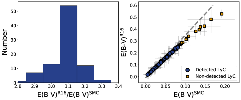
Figure 14: The impact of the assumed extinction law on the fitted attenuation parameter. Left Panel: Histogram of the ratio of the attenuation parameters derived using the Reddy et al. (2016) (R16) and the SMC laws. This ratio peaks strongly at a value of 3.1. Right Panel: The correlation of the attenuation parameter for the R16 and SMC extinction laws for the LyC detected (blue circles) and non-detected (gold squares) samples. Overplotted as a gray dashed line is an analytical fit to this scaling (Equation 22).

The fitted E(B-V) has one of the most statistically significant correlations with $f_{\rm esc,LyC}$ (Saldana-Lopez et al., 2022). E(B-V) also strongly determines the $\beta_{\rm obs}^{1550}$ of the LzLCS (see section 4), but the E(B-V) parameter depends on the assumed extinction law. As such an important diagnostic quantity, here we discuss the assumptions underpinning the chosen extinction law and its impact on the inferred spectral shape of the stellar continuum models and the E(B-V) parameter.

In Saldana-Lopez et al. (2022), we tested the impact of the assumed extinction law. We found that varying the extinction law from the Reddy et al. (2016) to an extrapolation of the SMC law (Prevot et al., 1984) did not impact the model parameters that set the intrinsic shape: age and metallicity. Therefore, the intrinsic stellar population properties do not appreciably change with different extinction laws. However, the absolute values of the individual fitted $X_{j}$ values do change because the SMC extinction law is both steeper and has larger $k(\lambda)$ values than the Reddy et al. (2016) law. This is likely because the FUV stellar spectral features (e.g. Figure 1) constrain the intrinsic properties of the stellar population. This sets the intrinsic shape of the stellar continuum, $\beta_{\rm int}^{1550}$, and E(B-V) is varied, using the assumed reddening law, to reconcile $\beta_{\rm int}^{1550}$ to $\beta_{\rm obs}^{1550}$ (see section 4).

Comparing the different extinction laws provides a prescription to convert $\beta_{\rm obs}^{1550}$ into E(B-V) for different extinction laws. The left panel of Figure 14 shows the ratio of the E(B-V) assuming a Reddy et al. (2016) (E(B-V)^R16) to the E(B-V) assuming an extrapolation of the SMC law (E(B-V)^SMC). The ratio of the two E(B-V) values peaks strongly with a median value of 3.09 and a standard deviation of 0.09, much smaller than the median 0.7 mag uncertainty on the measured ratio. The right panel of Figure 14 shows the strong correlation between the two E(B-V) values.

The E(B-V) differences derived with different reddening laws can be estimated analytically. First, we approximate the ratio of the observed flux at two wavelengths (F($\lambda^{1}$) and F($\lambda^{1}$)) as the ratio of the intrinsic flux times an unknown attenuation factor as

$$\frac{F(\lambda^{1})}{F(\lambda^{2})}=\frac{F_{i}(\lambda^{1})}{F_{i}(\lambda^{2})}e^{-E(B-V)\left[k(\lambda^{1})-k(\lambda^{2})\right]}=Re^{-E(B-V)\Delta k},$$ (19)

where we have defined $R$ as the intrinsic flux ratio at wavelengths 1 and 2, and $\Delta k=k(\lambda^{1})-k(\lambda^{1})$ is the difference of the extinction law at two wavelengths ($\lambda^{1}$ and $\lambda^{2}$). Regardless of the assumed law, the observed flux densities must be equal at the two wavelengths. Numerically, this means that

$$\frac{F^{\rm R16}(\lambda^{1})}{F^{\rm R16}(\lambda^{2})}=\frac{F^{\rm SMC}(\lambda^{1})}{F^{\rm SMC}(\lambda^{2})}.$$ (20)

Substituting in Equation 19 then suggests that E(B-V)^R16 is related to E(B-V)^SMC as

$$E(B-V)^{\rm R16}=\frac{\Delta k^{\rm SMC}}{\Delta k^{\rm R16}}E(B-V)^{\rm SMC}+\frac{1}{\Delta k^{\rm R16}}\ln{\frac{R^{\rm R16}}{R^{\rm SMC}}}$$ (21)

If we use 950 Å as wavelength 1 and 1200 Å as wavelength 2 (typical wavelengths used to fit the models of the LzLCS), we find that $\Delta k^{R16}=2.1$ and $\Delta k^{\rm SMC}=6.7$ such that the E(B-V) of the two laws is related as:

$$E(B-V)^{R16}=3.14\times E(B-V)^{\rm SMC}+0.47\ln{\frac{R^{\rm R16}}{R^{\rm SMC}}}$$ (22)

The slope of this line matches the median 3.09 found from the ratio of the two attenuation parameters (left panel of Figure 14). If we fix the slope of the line in Figure 14 to the theoretical ratio of $\Delta k^{\rm SMC}$/$\Delta k^{\rm R16}=3.14$, we find that $0.47\ln\left({R^{\rm R16}/R^{\rm SMC}}\right)=0.004$, implying that assuming an SMC law leads to an intrinsic FUV flux that is 1.01 times that of the Reddy et al. (2016) law. Thus, a good approximation for the conversion of the E(B-V) determined in the 950-1200 Å region with the Reddy et al. (2016) law to the SMC law is a constant factor of 3.1. This exercise illustrates how the individual reddening laws can be converted between each other, depending on the $\Delta k$ values of the individual extinction laws at their specific wavelengths. While we use the Reddy et al. (2016) law for the paper, Equation 21 can be used to convert E(B-V) to other dust extinction laws and derive the respective $\beta_{\rm obs}^{1550}$ values.

References

- Ahumada et al. (2020) Ahumada R., et al., 2020, ApJS, 249, 3
- Atek et al. (2018) Atek H., Richard J., Kneib J.-P., Schaerer D., 2018, MNRAS, 479, 5184
- Bañados et al. (2018) Bañados E., et al., 2018, Nature, 553, 473
- Becker & Bolton (2013) Becker G. D., Bolton J. S., 2013, MNRAS, 436, 1023
- Becker et al. (2001) Becker R. H., et al., 2001, AJ, 122, 2850
- Becker et al. (2021) Becker G. D., D’Aloisio A., Christenson H. M., Zhu Y., Worseck G., Bolton J. S., 2021, MNRAS, 508, 1853
- Berg et al. (2012) Berg D. A., et al., 2012, ApJ, 754, 98
- Bergvall et al. (2006) Bergvall N., Zackrisson E., Andersson B.-G., Arnberg D., Masegosa J., Östlin G., 2006, A&A, 448, 513
- Bhatawdekar & Conselice (2021) Bhatawdekar R., Conselice C. J., 2021, ApJ, 909, 144
- Borthakur et al. (2014) Borthakur S., Heckman T. M., Leitherer C., Overzier R. A., 2014, Science, 346, 216
- Bouwens et al. (2014) Bouwens R. J., et al., 2014, ApJ, 793, 115
- Bouwens et al. (2015) Bouwens R. J., et al., 2015, ApJ, 803, 34
- Bouwens et al. (2016) Bouwens R. J., Smit R., Labbé I., Franx M., Caruana J., Oesch P., Stefanon M., Rasappu N., 2016, ApJ, 831, 176
- Bouwens et al. (2021) Bouwens R. J., et al., 2021, AJ, 162, 47
- Bouwens et al. (2022) Bouwens R. J., Illingworth G. D., Ellis R. S., Oesch P. A., Stefanon M., 2022, arXiv e-prints, p. arXiv:2205.11526
- Calzetti (2013) Calzetti D., 2013, in Falcón-Barroso J., Knapen J. H., eds, , Secular Evolution of Galaxies. p. 419
- Calzetti et al. (1994) Calzetti D., Kinney A. L., Storchi-Bergmann T., 1994, ApJ, 429, 582
- Calzetti et al. (2000) Calzetti D., Armus L., Bohlin R. C., Kinney A. L., Koornneef J., Storchi-Bergmann T., 2000, ApJ, 533, 682
- Cardelli et al. (1989) Cardelli J. A., Clayton G. C., Mathis J. S., 1989, ApJ, 345, 245
- Chisholm et al. (2017) Chisholm J., Tremonti C. A., Leitherer C., Chen Y., 2017, MNRAS, 469, 4831
- Chisholm et al. (2018) Chisholm J., et al., 2018, A&A, 616, A30
- Chisholm et al. (2019) Chisholm J., Rigby J. R., Bayliss M., Berg D. A., Dahle H., Gladders M., Sharon K., 2019, ApJ, 882, 182
- Chisholm et al. (2020) Chisholm J., Prochaska J. X., Schaerer D., Gazagnes S., Henry A., 2020, MNRAS, 498, 2554
- Davis et al. (2021) Davis D., et al., 2021, ApJ, 920, 122
- Dayal et al. (2020) Dayal P., et al., 2020, MNRAS, 495, 3065
- De Barros et al. (2019) De Barros S., Oesch P. A., Labbé I., Stefanon M., González V., Smit R., Bouwens R. J., Illingworth G. D., 2019, MNRAS,
- Dunlop et al. (2013) Dunlop J. S., et al., 2013, MNRAS, 432, 3520
- Eldridge et al. (2017) Eldridge J. J., Stanway E. R., Xiao L., McClelland L. A. S., Taylor G., Ng M., Greis S. M. L., Bray J. C., 2017, Publications of the Astron. Soc. of Australia, 34, e058
- Endsley & Stark (2022) Endsley R., Stark D. P., 2022, MNRAS, 511, 6042
- Endsley et al. (2021) Endsley R., Stark D. P., Chevallard J., Charlot S., 2021, MNRAS, 500, 5229
- Fan et al. (2006) Fan X., et al., 2006, AJ, 132, 117
- Faucher-Giguère (2020) Faucher-Giguère C.-A., 2020, MNRAS, 493, 1614
- Faucher-Giguère et al. (2009) Faucher-Giguère C.-A., Lidz A., Zaldarriaga M., Hernquist L., 2009, ApJ, 703, 1416
- Ferland et al. (2017) Ferland G. J., et al., 2017, Rev. Mex. Astron. Astrofis., 53, 385
- Finkelstein et al. (2012) Finkelstein S. L., et al., 2012, ApJ, 756, 164
- Finkelstein et al. (2015) Finkelstein S. L., et al., 2015, ApJ, 810, 71
- Finkelstein et al. (2019) Finkelstein S. L., et al., 2019, ApJ, 879, 36
- Finkelstein et al. (2021) Finkelstein S. L., et al., 2021, arXiv e-prints, p. arXiv:2106.13813
- Finkelstein et al. (2022) Finkelstein S. L., et al., 2022, ApJ, 928, 52
- Fitzpatrick (1999) Fitzpatrick E. L., 1999, PASP, 111, 63
- Fletcher et al. (2019) Fletcher T. J., Tang M., Robertson B. E., Nakajima K., Ellis R. S., Stark D. P., Inoue A., 2019, ApJ, 878, 87
- Flury et al. (2022a) Flury S. R., et al., 2022a, ApJS, 260, 1
- Flury et al. (2022b) Flury S. R., et al., 2022b, ApJ, 930, 126
- Fontanot et al. (2007) Fontanot F., Cristiani S., Monaco P., Nonino M., Vanzella E., Brandt W. N., Grazian A., Mao J., 2007, A&A, 461, 39
- Gazagnes et al. (2018) Gazagnes S., Chisholm J., Schaerer D., Verhamme A., Rigby J. R., Bayliss M., 2018, A&A, 616, A29
- Gazagnes et al. (2020) Gazagnes S., Chisholm J., Schaerer D., Verhamme A., Izotov Y., 2020, A&A, 639, A85
- Gnedin (2000) Gnedin N. Y., 2000, ApJ, 542, 535
- Green et al. (2012) Green J. C., et al., 2012, ApJ, 744, 60
- Green et al. (2018) Green G. M., et al., 2018, MNRAS, 478, 651
- Harikane et al. (2018) Harikane Y., et al., 2018, ApJ, 859, 84
- Hayes et al. (2011) Hayes M., Schaerer D., Östlin G., Mas-Hesse J. M., Atek H., Kunth D., 2011, ApJ, 730, 8
- Henry et al. (2018) Henry A., Berg D. A., Scarlata C., Verhamme A., Erb D., 2018, ApJ, 855, 96
- Hopkins et al. (2008) Hopkins P. F., Hernquist L., Cox T. J., Kereš D., 2008, ApJS, 175, 356
- Hutchison et al. (2019) Hutchison T. A., et al., 2019, ApJ, 879, 70
- Inoue et al. (2014) Inoue A. K., Shimizu I., Iwata I., Tanaka M., 2014, MNRAS, 442, 1805
- Izotov et al. (2016a) Izotov Y. I., Schaerer D., Thuan T. X., Worseck G., Guseva N. G., Orlitová I., Verhamme A., 2016a, MNRAS, 461, 3683
- Izotov et al. (2016b) Izotov Y. I., Orlitová I., Schaerer D., Thuan T. X., Verhamme A., Guseva N. G., Worseck G., 2016b, Nature, 529, 178
- Izotov et al. (2018a) Izotov Y. I., Schaerer D., Worseck G., Guseva N. G., Thuan T. X., Verhamme A., Orlitová I., Fricke K. J., 2018a, MNRAS, 474, 4514
- Izotov et al. (2018b) Izotov Y. I., Worseck G., Schaerer D., Guseva N. G., Thuan T. X., Fricke A. V., Orlitová I., 2018b, MNRAS, 478, 4851
- Izotov et al. (2021) Izotov Y. I., Worseck G., Schaerer D., Guseva N. G., Chisholm J., Thuan T. X., Fricke K. J., Verhamme A., 2021, MNRAS, 503, 1734
- Jaskot & Oey (2014) Jaskot A. E., Oey M. S., 2014, ApJ, 791, L19
- Ji et al. (2020) Ji Z., et al., 2020, ApJ, 888, 109
- Jiang et al. (2022) Jiang L., et al., 2022, arXiv e-prints, p. arXiv:2206.07825
- Katz et al. (2022) Katz H., et al., 2022, MNRAS,
- Kelly (2007) Kelly B. C., 2007, ApJ, 665, 1489
- Kewley et al. (2006) Kewley L. J., Groves B., Kauffmann G., Heckman T., 2006, MNRAS, 372, 961
- Kulkarni et al. (2019a) Kulkarni G., Keating L. C., Haehnelt M. G., Bosman S. E. I., Puchwein E., Chardin J., Aubert D., 2019a, MNRAS, 485, L24
- Kulkarni et al. (2019b) Kulkarni G., Worseck G., Hennawi J. F., 2019b, MNRAS, 488, 1035
- Leitet et al. (2011) Leitet E., Bergvall N., Piskunov N., Andersson B.-G., 2011, A&A, 532, A107
- Leitherer et al. (1999) Leitherer C., et al., 1999, ApJS, 123, 3
- Leitherer et al. (2010) Leitherer C., Ortiz Otálvaro P. A., Bresolin F., Kudritzki R.-P., Lo Faro B., Pauldrach A. W. A., Pettini M., Rix S. A., 2010, ApJS, 189, 309
- Leitherer et al. (2016) Leitherer C., Hernandez S., Lee J. C., Oey M. S., 2016, ApJ, 823, 64
- Livermore et al. (2017) Livermore R. C., Finkelstein S. L., Lotz J. M., 2017, ApJ, 835, 113
- Madau & Dickinson (2014) Madau P., Dickinson M., 2014, ARA&A, 52, 415
- Madau & Haardt (2015) Madau P., Haardt F., 2015, ApJ, 813, L8
- Madau et al. (1999) Madau P., Haardt F., Rees M. J., 1999, ApJ, 514, 648
- Mainali et al. (2018) Mainali R., et al., 2018, MNRAS, 479, 1180
- Makan et al. (2021) Makan K., Worseck G., Davies F. B., Hennawi J. F., Prochaska J. X., Richter P., 2021, ApJ, 912, 38
- Mannucci et al. (2010) Mannucci F., Cresci G., Maiolino R., Marconi A., Gnerucci A., 2010, MNRAS, 408, 2115
- Marques-Chaves et al. (2021) Marques-Chaves R., Schaerer D., Álvarez-Márquez J., Colina L., Dessauges-Zavadsky M., Pérez-Fournon I., Saldana-Lopez A., Verhamme A., 2021, MNRAS, 507, 524
- Martin et al. (2005) Martin D. C., et al., 2005, ApJ, 619, L1
- Maseda et al. (2020) Maseda M. V., et al., 2020, MNRAS, 493, 5120
- Mason et al. (2019) Mason C. A., Naidu R. P., Tacchella S., Leja J., 2019, MNRAS, 489, 2669
- Matsuoka et al. (2018) Matsuoka Y., et al., 2018, ApJ, 869, 150
- Matthee et al. (2021) Matthee J., et al., 2021, MNRAS, 505, 1382
- Matthee et al. (2022) Matthee J., et al., 2022, MNRAS, 512, 5960
- Mauerhofer et al. (2021) Mauerhofer V., Verhamme A., Blaizot J., Garel T., Kimm T., Michel-Dansac L., Rosdahl J., 2021, A&A, 646, A80
- McGaugh (1991) McGaugh S. S., 1991, The Astrophysical Journal, 380, 140
- McLeod et al. (2016) McLeod D. J., McLure R. J., Dunlop J. S., 2016, MNRAS, 459, 3812
- Mehta et al. (2017) Mehta V., et al., 2017, ApJ, 838, 29
- Miralda-Escudé & Rees (1994) Miralda-Escudé J., Rees M. J., 1994, MNRAS, 266, 343
- Naidu et al. (2020) Naidu R. P., Tacchella S., Mason C. A., Bose S., Oesch P. A., Conroy C., 2020, ApJ, 892, 109
- Naidu et al. (2022) Naidu R. P., et al., 2022, MNRAS, 510, 4582
- Nakajima & Ouchi (2014) Nakajima K., Ouchi M., 2014, MNRAS, 442, 900
- Newville et al. (2014) Newville M., Stensitzki T., Allen D. B., Ingargiola A., 2014, LMFIT: Non-Linear Least-Square Minimization and Curve-Fitting for Python, doi:10.5281/zenodo.11813
- Oesch et al. (2018) Oesch P. A., Bouwens R. J., Illingworth G. D., Labbé I., Stefanon M., 2018, ApJ, 855, 105
- Ouchi et al. (2009) Ouchi M., et al., 2009, ApJ, 696, 1164
- Pahl et al. (2021) Pahl A. J., Shapley A., Steidel C. C., Chen Y., Reddy N. A., 2021, MNRAS, 505, 2447
- Pilyugin et al. (2006) Pilyugin L. S., Vílchez J. M., Thuan T. X., 2006, MNRAS, 370, 1928
- Planck Collaboration et al. (2016) Planck Collaboration et al., 2016, A&A, 596, A108
- Popping & Péroux (2022) Popping G., Péroux C., 2022, MNRAS, 513, 1531
- Popping et al. (2017) Popping G., Somerville R. S., Galametz M., 2017, MNRAS, 471, 3152
- Prevot et al. (1984) Prevot M. L., Lequeux J., Maurice E., Prevot L., Rocca-Volmerange B., 1984, A&A, 132, 389
- Raiter et al. (2010) Raiter A., Schaerer D., Fosbury R. A. E., 2010, A&A, 523, A64
- Reddy et al. (2016) Reddy N. A., Steidel C. C., Pettini M., Bogosavljević M., 2016, ApJ, 828, 107
- Redwine et al. (2016) Redwine K., et al., 2016, PASP, 128, 105006
- Rémy-Ruyer et al. (2013) Rémy-Ruyer A., et al., 2013, A&A, 557, A95
- Ricci et al. (2017) Ricci F., Marchesi S., Shankar F., La Franca F., Civano F., 2017, MNRAS, 465, 1915
- Rivera-Thorsen et al. (2017) Rivera-Thorsen T. E., Östlin G., Hayes M., Puschnig J., 2017, ApJ, 837, 29
- Rivera-Thorsen et al. (2019) Rivera-Thorsen T. E., et al., 2019, Science, 366, 738
- Roberts-Borsani et al. (2021) Roberts-Borsani G., Morishita T., Treu T., Leethochawalit N., Trenti M., 2021, arXiv e-prints, p. arXiv:2106.06544
- Robertson et al. (2013) Robertson B. E., et al., 2013, ApJ, 768, 71
- Robertson et al. (2015) Robertson B. E., Ellis R. S., Furlanetto S. R., Dunlop J. S., 2015, ApJ, 802, L19
- Rosdahl et al. (2018) Rosdahl J., et al., 2018, MNRAS, 479, 994
- Rutkowski et al. (2017) Rutkowski M. J., et al., 2017, ApJ, 841, L27
- Saldana-Lopez et al. (2022) Saldana-Lopez A., et al., 2022, arXiv e-prints, p. arXiv:2201.11800
- Schaerer et al. (2022) Schaerer D., et al., 2022, A&A, 658, L11
- Shapley et al. (2016) Shapley A. E., Steidel C. C., Strom A. L., Bogosavljević M., Reddy N. A., Siana B., Mostardi R. E., Rudie G. C., 2016, ApJ, 826, L24
- Shen et al. (2020) Shen X., Hopkins P. F., Faucher-Giguère C.-A., Alexander D. M., Richards G. T., Ross N. P., Hickox R. C., 2020, MNRAS, 495, 3252
- Shull et al. (2012) Shull J. M., Harness A., Trenti M., Smith B. D., 2012, ApJ, 747, 100
- Skillman (1989) Skillman E. D., 1989, The Astrophysical Journal, 347, 883
- Stanway & Eldridge (2018) Stanway E. R., Eldridge J. J., 2018, MNRAS, 479, 75
- Stark et al. (2015) Stark D. P., et al., 2015, MNRAS, 454, 1393
- Stefanon et al. (2022) Stefanon M., Bouwens R. J., Illingworth G. D., Labbé I., Oesch P. A., Gonzalez V., 2022, arXiv e-prints, p. arXiv:2204.02986
- Steidel et al. (2018) Steidel C. C., Bogosavljević M., Shapley A. E., Reddy N. A., Rudie G. C., Pettini M., Trainor R. F., Strom A. L., 2018, ApJ, 869, 123
- Tacchella et al. (2021) Tacchella S., et al., 2021, arXiv e-prints, p. arXiv:2111.05351
- Tang et al. (2019) Tang M., Stark D. P., Chevallard J., Charlot S., 2019, MNRAS, 489, 2572
- Trebitsch et al. (2017) Trebitsch M., Blaizot J., Rosdahl J., Devriendt J., Slyz A., 2017, MNRAS, 470, 224
- Trebitsch et al. (2021) Trebitsch M., et al., 2021, A&A, 653, A154
- Tremonti et al. (2004) Tremonti C. A., et al., 2004, ApJ, 613, 898
- Vanzella et al. (2016) Vanzella E., et al., 2016, ApJ, 825, 41
- Vasei et al. (2016) Vasei K., et al., 2016, ApJ, 831, 38
- Verhamme et al. (2015) Verhamme A., Orlitová I., Schaerer D., Hayes M., 2015, A&A, 578, A7
- Vilchez & Pagel (1988) Vilchez J. M., Pagel B. E. J., 1988, Monthly Notices of the Royal Astronomical Society, 231, 257
- Wang et al. (2019) Wang B., Heckman T. M., Leitherer C., Alexandroff R., Borthakur S., Overzier R. A., 2019, ApJ, 885, 57
- Wang et al. (2021) Wang B., et al., 2021, ApJ, 916, 3
- Wilkins et al. (2016) Wilkins S. M., Bouwens R. J., Oesch P. A., Labbé I., Sargent M., Caruana J., Wardlow J., Clay S., 2016, MNRAS, 455, 659
- Witstok et al. (2021) Witstok J., Smit R., Maiolino R., Curti M., Laporte N., Massey R., Richard J., Swinbank M., 2021, MNRAS, 508, 1686
- Worseck et al. (2016) Worseck G., Prochaska J. X., Hennawi J. F., McQuinn M., 2016, ApJ, 825, 144
- Xu et al. (2022) Xu X., et al., 2022, arXiv e-prints, p. arXiv:2205.11317
- Yue et al. (2018) Yue B., et al., 2018, ApJ, 868, 115
- Yung et al. (2019) Yung L. Y. A., Somerville R. S., Finkelstein S. L., Popping G., Davé R., 2019, MNRAS, 483, 2983
- Yung et al. (2020) Yung L. Y. A., Somerville R. S., Popping G., Finkelstein S. L., 2020, MNRAS, 494, 1002
- Yung et al. (2021) Yung L. Y. A., Somerville R. S., Finkelstein S. L., Hirschmann M., Davé R., Popping G., Gardner J. P., Venkatesan A., 2021, MNRAS, 508, 2706
- Zackrisson et al. (2013) Zackrisson E., Inoue A. K., Jensen H., 2013, ApJ, 777, 39