The Evolution of Lyman Alpha Emitter Line Widths from $z$=5.7 to $z$=6.6

Abstract

Recent evidence suggests that high-redshift Ly$\alpha$ emitting galaxies (LAEs) with $\log L({\rm Ly}\alpha)>43.5~{}{\rm erg\ s}^{-1}$, referred to as ultraluminous LAEs (ULLAEs), may show less evolution than lower-luminosity LAEs in the redshift range $z=5.7$–6.6. Here we explore the redshift evolution of the velocity widths of the Ly$\alpha$ emission lines in LAEs over this redshift interval. We use new wide-field, narrowband observations from Subaru/Hyper Suprime-Cam to provide a sample of 24 $z=6.6$ and 12 $z=5.7$ LAEs with $\log L({\rm Ly}\alpha)>43~{}{\rm erg\ s}^{-1}$, all of which have follow-up spectroscopy from Keck/DEIMOS. Combining with archival lower-luminosity data, we find a significant narrowing of the Ly$\alpha$ lines in LAEs at $\log L({\rm Ly}\alpha)<43.25~{}{\rm erg\ s}^{-1}$—somewhat lower than the usual ULLAE definition—at $z=6.6$ relative to those at $z=5.7$, but we do not see this in higher-luminosity LAEs. As we move to higher redshifts, the increasing neutrality of the intergalactic medium should increase the scattering of the Ly$\alpha$ lines, making them narrower. The absence of this effect in the higher-luminosity LAEs suggests they may lie in more highly ionized regions, self-shielding from the scattering effects of the intergalactic medium.

1 Introduction

Ly$\alpha$ emitting galaxies (LAEs) may provide our current strongest probe of the epoch of reionization, which occurred at $z\sim 7$. The evolution of LAEs can provide powerful diagnostics of the physics of the ionization of the intergalactic medium (IGM), the sources of the ionizing photons, and the structure of the ionized regions in the IGM. As the neutral hydrogen fraction in the IGM increases with increasing redshift, we expect that Ly$\alpha$ emission lines should become narrower and less luminous and that only the red wings of the lines should be seen (see, e.g., Hayes et al. 2021 and references therein). At $z>5.5$, this is observed for LAEs with Ly$\alpha$ luminosities $L(\textrm{Ly$\alpha$})<10^{43.5}$ erg s^-1.

However, the advent of giant imagers, such as Subaru/Hyper Suprime-Cam (HSC; Miyazaki et al., 2018), has allowed an expansion in the range of luminosities that can be observed, making it possible to probe the rarer ultraluminous LAEs ($L(\textrm{Ly$\alpha$})>10^{43.5}$ erg s^-1; ULLAEs). Based on the mapping of these sources, recent work has suggested that ULLAEs do not show such evolution.

One route for probing the evolution of LAEs at these high redshifts is by measuring their luminosity functions (LFs). Santos et al. (2016) were the first to claim no evolution in their photometric LAE LFs at the ultraluminous end after observing that their $z=5.7$ and $z=6.6$ LFs converged near $\log L(\textrm{Ly$\alpha$})\approx 43.6$ erg s^-1. They interpreted this result as evidence that the most luminous LAEs formed ionized bubbles around themselves, thereby becoming visible at earlier redshifts than lower-luminosity LAEs. The normalizations of the Santos et al. (2016) LFs have been questioned in subsequent papers (Konno et al., 2018; Taylor et al., 2020). However, recent analyses by Taylor et al. (2020, 2021) and Ning et al. (2022) are also consistent with no evolution in the ULLAE LF, though the results are not highly significant, as we discuss further in the summary.

If the most luminous LAEs do indeed generate ionized bubbles, then theoretical modeling can be used to infer key properties of the galaxies, such as the escape fraction of ionizing photons (e.g., Gronke et al., 2021).

The formation of ionized bubbles is also suggested by the discovery of double-peaked spectra in some ULLAEs at $z=6.6$. While Ly$\alpha$ line profiles at $z\sim 3$ show double-peaked spectra (both red and blue peaks) in $\sim$30% of cases (Kulas et al., 2012), at $z>5$, it was expected that the blue peak should always be scattered away by the neutral portion of the IGM (Hu et al., 2010; Hayes et al., 2021), leaving a single peak featuring a sharp blue break and an extended red wing. However, Hu et al. (2016) and Songaila et al. (2018) reported $z=6.6$ double-peaked ULLAEs in the COSMOS (COLA1) and North Ecliptic Pole (NEP) (NEPLA4) fields, respectively. More recently, Meyer et al. (2021) found a $z=6.8$ double-peaked LAE at a luminosity of $\log L(\textrm{Ly$\alpha$})=42.99$ erg s^-1 in the A370p field (A370p_z1), and Bosman et al. (2020) found a $z=5.8$ double-peaked LAE at a luminosity of $\log L(\textrm{Ly$\alpha$})=43.03$ erg s^-1 in a quasar proximity zone (Aerith B). In a theoretical analysis, Gronke et al. (2021) showed that ionized bubbles around such objects can allow the double-peaked structure to be seen.

In the present paper, we investigate another route for probing the evolution of LAEs at these high redshifts, namely, by mapping the velocity widths of the Ly$\alpha$ profiles as a function of redshift and luminosity. We use wide-field narrowband observations of the NEP made with Subaru/HSC to develop substantial samples of luminous LAEs, all of which have follow-up spectroscopy from Keck/DEIMOS. In combination with lower-luminosity observations from Hu et al. (2010) (note that, for simplicity, we will refer to their $z=6.5$ sample as being at $z=6.6$), this provides a set of homogeneously observed velocity profiles over a wide range of luminosities at $z=5.7$ and $z=6.6$.

We assume $\Omega_{M}=0.3$, $\Omega_{\Lambda}=0.7$, and $H_{0}=70$ km s^-1 Mpc^-1 throughout. All magnitudes are given in the AB magnitude system, where an AB magnitude is defined by $m_{AB}=-2.5\log f_{\nu}-48.60$. Here $f_{\nu}$ is the flux of the source in units of ergs cm^-2 s^-1 Hz^-1.

2 Data

2.1 Target selection

Our LAE sample is primarily drawn from the HEROES survey centered on the NEP (Songaila et al., 2018). The HEROES observations in the optical were made with Subaru/HSC and were reduced with the hscPipe software, which was also used to generate the catalogs (A. Taylor et al. 2022, in preparation). For each object, we computed the magnitudes using $2^{\prime\prime}$ diameter apertures, and we corrected these to total magnitudes using the median offset between $2^{\prime\prime}$ and $4^{\prime\prime}$ apertures. These offsets are typically around -0.2 mag. The corrected aperture magnitudes match well to Kron magnitudes measured on the galaxies. The HEROES data have very high-quality spatial resolution, about $0.5^{\prime\prime}$–$0.6^{\prime\prime}$ full width at half maximum (FWHM) for most of the colors throughout most of the field.

The full HSC observations of HEROES cover $50.2~{}{\rm deg}^{2}$ in 5 broadbands: $g$: 27.3, $r$: 26.9, $i$: 26.5, $z$: 26.0, and $Y$: 25.3, where the numbers are the median $1\sigma$ noise across the field in the corrected $2\arcsec$ diameter apertures. The field is also imaged in two narrowband filters, NB816 and NB921, with $1\sigma$ depths of 25.9 and 25.7, respectively.

We also obtained deeper observations around the JWST Time Domain Field (JTDF) (Jansen & Windhorst, 2018). The JTDF is a $14\arcmin$ diameter field that lies within the footprint of HEROES. It will be intensively observed with JWST, as well as with HST, Chandra, and ground-based telescopes. The NB921 observations of this region cover $2.1~{}{\rm deg}^{2}$ and have a median $1\sigma$ depth of 26.2, or about 0.5 mag deeper than the average sensitivity.

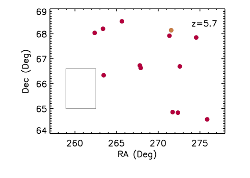
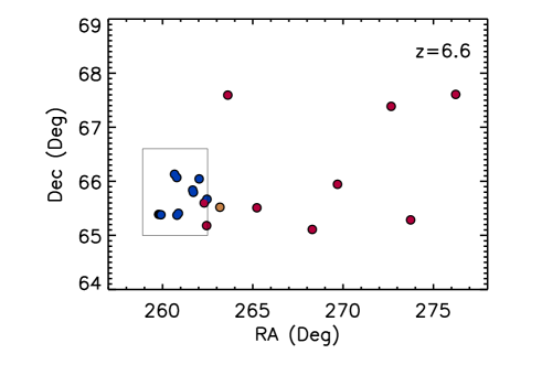
Figure 1: (Left) The $z=5.7$ HEROES LAE sample (Table 1; red circles). (Right) The $z=6.6$ HEROES (Table 2; red circles) and JTDF (Table 3; blue circles) LAE samples. In both panels, the new Subaru/HSC data surrounding the JTDF field are marked with a rectangle, and gold circles show spectroscopically detected AGNs at the given redshifts.

The selection of the $z=6.6$ LAEs from the NB921 imaging is described in Taylor et al. (2020), and the selection of the $z=5.7$ LAEs from the NB816 imaging is described in Taylor et al. (2021). These papers also describe the computation of the Ly$\alpha$ line luminosities from the narrowband magnitudes. While the exact conversion depends on the position of the Ly$\alpha$ line on the filter, and hence on the redshift, the $5\sigma\log L(\textrm{Ly$\alpha$})$ limit is roughly 42.4 erg s^-1 at $z=5.7$ and 43.0 erg s^-1 at $z=6.6$. The $5\sigma\log L(\textrm{Ly$\alpha$})$ limit in the JTDF field is 42.5 erg s^-1 at $z=6.6$.

We summarize the $z=5.7$ LAE sample from Taylor et al. (2021) in Table 1, the $z=6.6$ LAE sample from Taylor et al. (2020) in Table 2, and the new JTDF LAE sample from this work in Table 3. The selection of the JTDF LAE sample precisely follows the methods used in the two previous papers. In Table 2, we added three sources from the COSMOS field: COLA1 from Hu et al. (2016) and CR7 and MASOSA from Sobral et al. (2015) and Matthee et al. (2015). We also added one source (VR7) from the SSA22 field (Matthee et al., 2017) and one source (GN-LA1) from the GOODS-N field (Hu et al., 2010). These add additional high-luminosity LAEs where we have high-quality Keck/DEIMOS spectra obtained in the same configurations as for the LAEs in the NEP field.

In the tables, we only include sources whose redshifts have been confirmed by subsequent spectroscopy. We give the source name, the R.A. and decl., the redshift corresponding to the peak of the Ly$\alpha$ line, the $\log L(\textrm{Ly$\alpha$})$, and the FWHM. Note that we quote the observed luminosity. We have made no attempt to correct for the intergalactic transmission, and the intrinsic luminosity could be higher, possibly by a factor of two or more (e.g., Hu et al. 2010). However, estimating this correction would not be easy, given the possible presence of ionized bubbles surrounding these objects, and we do not do so here. We show the locations of the LAEs on the HEROES and JTDF fields in Figure 1.

In the present paper, we compare the above samples with less luminous samples from Hu et al. (2010). We re-reduced their spectra and included new data that we obtained subsequently.

For consistency, we analyze all the samples using the asymmetric fitting procedures described in Section 3.

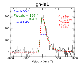
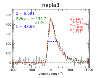
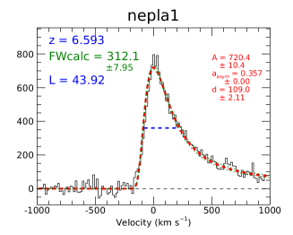
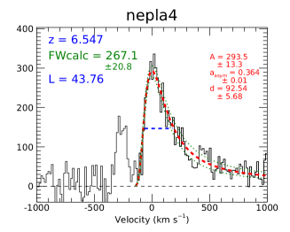
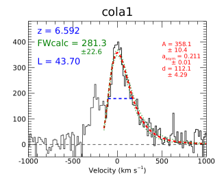
Figure 2: Examples of asymmetric fits to $z=6.6$ LAEs. The top three panels show fits to three LAEs with a range of luminosities. The lower two panels show the two double-peaked ULLAEs, where we have fitted to only the red wing. In all cases, the red dashed curve shows the fit to the data (black), and the green dotted curves show the $1\sigma$ errors. The adopted widths based on the fits, FWcalc in km s^-1, are listed in green and are shown as the blue dashed lines. The redshift and $\log L(\textrm{Ly$\alpha$})$ in erg s^-1 values are listed in blue, and the fitting parameters from Equation 1 are listed in red. Because of the uncertainties in the spectrophotometric calibration, the y-axis shows the flux in arbitrary units.

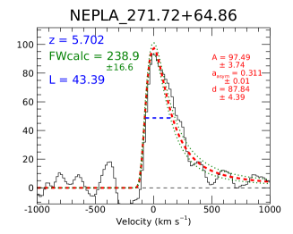
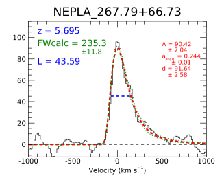
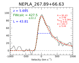
Figure 3: Examples of asymmetric fits to $z=5.7$ LAEs. The notation is the same as in Figure 2.

2.2 Spectroscopy

We obtained spectroscopic observations with the Keck/DEIMOS spectrograph for all of the sources in Tables 1, 2, and 3, though we have previously reported some of them in Songaila et al. (2018) and in Taylor et al. (2020, 2021). We configured DEIMOS using $1\arcsec$ slits and the 830G grating, which has high throughput at 9000 Å and provides a resolution of $R=2550$. We took three 20 min sub-exposures for each slitmask, dithering $\pm 1\farcs 5$ along the slits for improved sky subtraction and to minimize CCD systematics. The minimum total exposure on an individual LAE was 1 hr, while most were observed for 2–3 hr. GN-LA1 in the intensely observed GOODS-N field has 14 hr of exposure.

We reduced the data using the standard pipeline from Cowie et al. (1996). We performed an initial pixel-by-pixel sky subtraction by combining the three dithered exposures and subtracting the minimal value recorded by each pixel. Next, we median combined the three dithered frames, adjusting for the $\pm 1\farcs 5$ offsets. We rejected cosmic rays using a $3\times 3$ pixel median rejection spatial filter, and we quantified and corrected for geometric distortions in the spectra using pre-selected bright continuum sources from the slitmask. Lastly, we used the observed sky lines to calibrate the wavelength scale and to perform a final sky subtraction.

In Figure 2, we show the spectra of three $z=6.6$ LAEs with a range of luminosities, along with the two double-peaked ULLAEs. In Figure 3, we show the spectra of three $z=5.7$ LAEs with a range of luminosities. There is no sign of active galactic nucleus (AGN) activity, such as [NV], in any of the LAE spectra. The selection method does pick out a small number of AGNs at these redshifts, but they are easily distinguished based on their spectra. There is one AGN in each sample (see Figure 1).

3 Line Width Measurements

Following Claeyssens et al. (2019) and Shibuya et al. (2014), we fitted the LAE Ly$\alpha$ lines with an asymmetric profile,

$$f(\lambda)=A\exp\left(-\frac{\Delta v^{2}}{2(a_{\rm asym}(\Delta v)+d)^{2}}\right)\,,$$ (1)

where $A$ is the normalization, $\Delta v$ is the velocity relative to the peak of the Ly$\alpha$ profile, $a_{\rm asym}$ controls the asymmetry, and $d$ controls the line width. We fitted this function to the Ly$\alpha$ lines in the three samples listed in Tables 1, 2, and 3 and to the Hu et al. (2010) sample using the IDL fitting routine MPFIT of Markwardt (2009). In terms of these free parameters, the width of the line is

$${\rm FWHM}=\frac{2\sqrt{2\ln 2}\ d}{(1-2\ln 2\ a_{\rm asym}^{2})}\,.$$ (2)

We show the fits for the LAEs in Figures 2 and 3. In each case, we show the model fit (red) overlaid on the spectrum (black). We list the fitted parameters from Equation 1 in red in each panel. For the sources with double peaks, we fitted only to the red side, as we show in the lower panels of Figure 2.

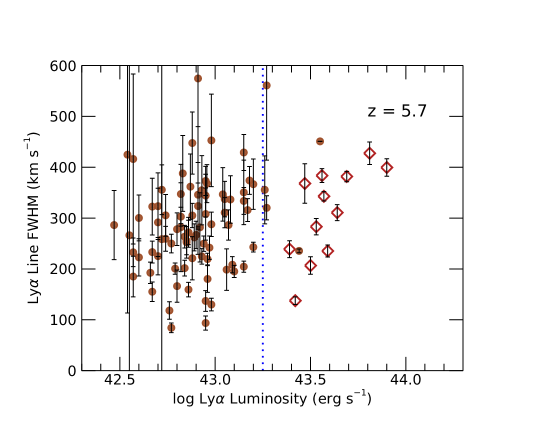
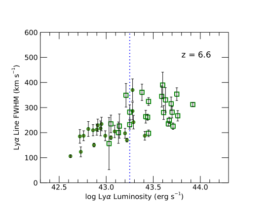
Figure 4: Ly$\alpha$ line FWHM vs. $\log L(\textrm{Ly$\alpha$})$ for the $z=5.7$ (left) data from Table 1 (open diamonds) and Hu et al. (2010) (solid circles), and for the $z=6.6$ (right) data from Tables 2 and 3 (open squares) and Hu et al. (2010) (solid circles). The figure shows the raw FWHM without a correction for the instrumental resolution. In both panels, the blue dotted vertical line shows our rough division of $\log L(\textrm{Ly$\alpha$})=43.25$ erg s^-1 between the lower- and higher-luminosity samples. In all cases, the uncertainties are $1\sigma$. We do not show the very large error bars on the most luminous Hu et al. (2010) object in the $z=5.7$ panel.

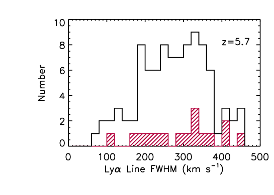
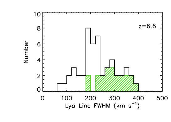
Figure 5: Histograms of the distributions of the line widths at $z=5.7$ (left) and $z=6.6$ (right) from Figure 4. In both panels, the open regions show the total samples, and the shaded regions show the higher-luminosity samples.

For each LAE, we computed the FWHM of the line and its error using the asymmetric profile fit. We call this FWcalc, which has units of km s^-1. We give this line width in green in each panel of Figures 2 and 3. We show the fitted FWHM as the blue dashed line. It is this quantity that we subsequently use in our analysis. However, we also directly measured the FWHM from the spectrum. The directly measured values are in broad agreement with our adopted FWHMs, but they have a slight bias to lower values, because they correspond to the first half-maximum intercept. It is for this reason that we prefer the fitted FWHMs.

We give the fitted FWHMs and their 1$\sigma$ errors in the final columns of Tables 1, 2, and 3. These values are not corrected for the instrument resolution, which has a FWHM of 117 km s^-1. However, most of the lines are very well resolved.

4 Discussion

In Figure 4, we plot Ly$\alpha$ line FWHM versus $\log L(\textrm{Ly$\alpha$})$ at $z=5.7$ (left) and at $z=6.6$ (right). The increase in the dynamical range of the measured Ly$\alpha$ luminosities reveals a new result. At the previously measured lower luminosities, the widths of the lines show a decrease with increasing redshift, but at the higher luminosities, the widths of the lines for the $z=5.7$ sample are comparable to the widths of the lines for the $z=6.6$ sample.

Based on the $z=6.6$ figure, we use a dividing line of $\log L(\textrm{Ly$\alpha$})=43.25$ erg s^-1 (blue dotted line) to separate roughly the data into lower- and higher-luminosity samples. There is some uncertainty in this value, which could lie in the 43.17 to 43.4 range. We are currently expanding the sample of intermediate luminosity LAEs, which should allow a better determination. However, we note that the analysis below is not sensitive to the exact choice.

Now we can quantify the result on the widths, which we do by redshift. At $z=5.7$, the median FWHM of the higher-luminosity sample ($\log L(\textrm{Ly$\alpha$})>43.25$ erg s^-1) is fairly comparable to that of the lower-luminosity sample ($\log L(\textrm{Ly$\alpha$})<43.25$ erg s^-1). There are 17 sources in the higher-luminosity sample, which includes a very small number of sources from Hu et al. (2010) (solid circles). The median FWHM for this sample is 320 km s^-1, with a standard error of 26 km s^-1 computed using the bootstrap method. For the 79 sources in the lower-luminosity sample, which come entirely from Hu et al. (2010), the median FWHM is 278 km s^-1, with a standard error of 12 km s^-1.

In contrast, at $z=6.6$, the median FWHM of the higher-luminosity sample is considerably larger than that of the lower-luminosity sample. This is true for both the sample of Tables 2 and 3 (open squares) and the sample of Hu et al. (2010) (solid circles) in the rather limited overlap region. For the 21 sources in the higher-luminosity sample, the median FWHM is 281 km s^-1, with a standard error of 21 km s^-1. For the 30 $z=6.6$ sources in the lower-luminosity sample, the median FWHM is 197 km s^-1, with a standard error of 9 km s^-1.

In Figure 5, we show the histograms of the distributions of the line widths at $z=5.7$ (left) and $z=6.6$ (right) for the total (open regions) and higher-luminosity (shaded regions) samples of Figure 4. As expected, at $z=5.7$, the lower- and higher-luminosity samples have very similar distributions. A Mann-Whitney test does not show a significant difference. However, at $z=6.6$, a Mann-Whitney test gives a probability of $<10^{-5}$ that the lower- and higher-luminosity samples have consistent distributions.

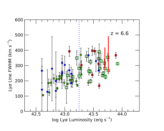
Figure 6: Ly$\alpha$ line FWHM vs. $\log L(\textrm{Ly$\alpha$})$ at $z=6.6$. The green symbols of the present sample (from Figure 4) are to be compared with the samples of Shibuya et al. (2018) (red squares) and Ouchi et al. (2010) (blue circles). For the two double-peaked ULLAEs (COLA1 and NEPLA4, see Figure 2), we show the range in FWHM when we include or exclude the blue wing (red bars).

Moreover, including the blue wings for the two double-peaked sources COLA1 and NEPLA4 would only make this difference more pronounced, since it would increase the higher-luminosity distribution. We illustrate this in Figure 6, where we again plot Ly$\alpha$ line FWHM versus $\log L(\textrm{Ly$\alpha$})$ for the $z=6.6$ samples of Figure 4 (green symbols). We use red vertical bars to show the range of FWHMs for COLA1 and NEPLA4 after excluding or including the blue wing.

For comparison, we also show in this figure measurements from Ouchi et al. (2010) (blue) and Shibuya et al. (2018) (red). Within the fairly substantial error bars on the Ouchi et al. (2010) data points, the present and archival data sets are broadly consistent. Note, however, that there is one archival lower-luminosity object (HSCJ160107$+$550720 at $\log L(\textrm{Ly$\alpha$})=43.08$ erg s^-1 in Shibuya et al., 2018) that has an unusually large width of 393 km s^-1.

Because of the different instruments employed and the different analysis techniques used in these papers versus the present work (namely, single Gaussian versus asymmetric profile fitting), we do not attempt to incorporate the Ouchi et al. (2010) and Shibuya et al. (2018) results into our analysis and instead restrict to the current homogeneous samples of Tables 1–3.

We can compare the lower- and higher-luminosity samples more directly by stacking the individual spectra. In Figure 7, we show the sum of the spectra at $z=5.7$ (left) and at $z=6.6$ (right) for the various samples. The shading shows the 68% confidence range calculated using the bootstrap method. The $z=5.7$ stacked spectra show close agreement between the lower- and higher-luminosity samples, with the higher-luminosity sample being only slightly wider, while the $z=6.6$ stacked spectra show the higher-luminosity sample being considerably wider. In all cases, the measured FWHMs of the stacks match well to the median FWHMs of the individual sources discussed above.

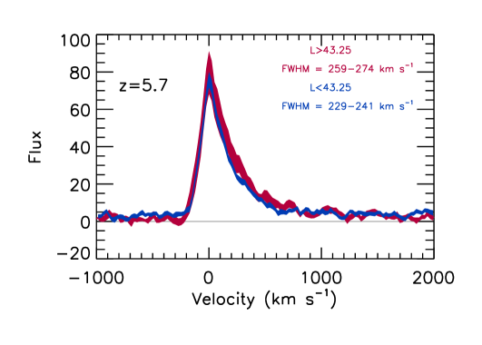
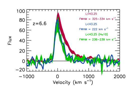
Figure 7: (Left) Stack of the $z=5.7$ emission-line spectra for the lower-luminosity ($\log L(\textrm{Ly$\alpha$})<43.25$ erg s^-1; blue curve) LAEs from Hu et al. (2010) and higher-luminosity ($\log L(\textrm{Ly$\alpha$})>43.25$ erg s^-1; red curve) LAEs of the present sample (Table 1). (Right) Stack of the $z=6.6$ emission-line spectra for the lower-luminosity (blue curve) and higher-luminosity (red curve) LAEs of the present sample (Tables 2 and 3). The green curve shows the stack for the lower-luminosity LAEs from Hu et al. (2010). (Note that the green and blue curves are based on a disjoint set of objects.) In both panels, the legends display 68% confidence ranges for the FWHMs, which were computed using the bootstrap method. These confidence ranges are also displayed through shading. In the right panel, the present $\log L(\textrm{Ly$\alpha$})<43.25$ erg s^-1 sample (blue curve) has too few objects to compute the error range.

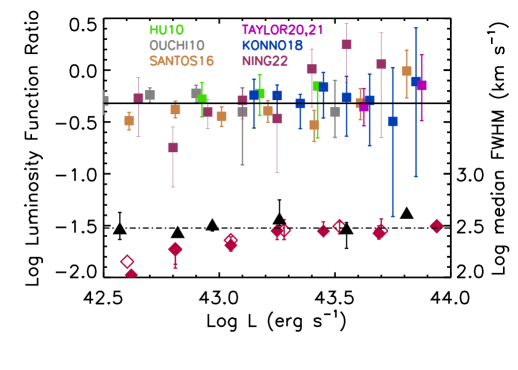
Figure 8: Logarithmic ratio of the LF at $z=6.6$ to that at $z=5.7$ for all published LAE LFs (solid squares color-coded according to the legend). The black solid line corresponds to a drop of 2.1 between the two redshifts, which roughly matches all of the measurements at lower luminosities. At the high-luminosity end, the measurements show a logarithmic ratio closer to 1, but the results are only marginally significant. The lower points (right-axis scale) show the median FWHMs at $z=6.6$ (red solid diamonds are the present data, while the red open diamonds also include the Shibuya et al. 2018 and Ouchi et al. 2010 data) and at $z=5.7$ (black solid triangles). The black dot-dashed line shows a value of 300 km s^-1, which roughly matches the entire $z=5.7$ sample and the $z=6.6$ higher-luminosity sample. All error bars are 68% confidence ranges.

5 Summary

We summarize our results in Figure 8, where we compare the evolution of the LFs with the evolution of the line widths. The solid squares show the ratio of the LF at $z=6.6$ to that at $z=5.7$ as reported by all of the groups who have measured the two LFs (Hu et al., 2010; Ouchi et al., 2010; Santos et al., 2016; Konno et al., 2018; Taylor et al., 2020, 2021; Ning et al., 2022). While there is substantial variation in the normalization of the LFs between the groups, the LF ratio is much more homogeneous. All of the measurements show a drop of about 2.1 in the $z=6.6$ LF from that at $z=5.7$. Only at the high-luminosity end is there a smaller drop, but although this result is seen in all the samples, it is somewhat marginal (see Taylor et al. 2021 for a more extended discussion).

By contrast, the evolution of the line widths is much more clear. The median FWHMs as a function of $\log L(\textrm{Ly$\alpha$})$ are shown as the black triangles ($z=5.7$) and the red diamonds ($z=6.6$). The solid diamonds include only the present data, while the open diamonds also include the data from Ouchi et al. (2010) and Shibuya et al. (2018). The $z=5.7$ values show no variation with luminosity, consistent with their lying in similarly ionized regions of the IGM. The $z=6.6$ values at higher luminosities are $\sim 300$ km s^-1, the same as the $z=5.7$ values at all luminosities. However, the $z=6.6$ values at lower luminosities show a highly significant drop, consistent with the higher-redshift sources lying in more neutral IGM.

We conclude that $z=6.6$ LAEs with observed luminosities $\log L(\textrm{Ly$\alpha$})>43.25~{}{\rm erg\ s}^{-1}$ mark ionized regions. The reason for this could be that the galaxies themselves are fully responsible for the ionization, but it is also possible that they are lying in regions where neighboring galaxies are producing sufficient ionization to allow the intrinsic galaxy profile to be seen.

While this seems the most likely explanation, there may be other possibilities. In particular, intrinsic line profile shapes may vary due to different physical conditions, dust extinction, or the age of the star formation burst (see, e.g., Verhamme et al. 2012, 2015; Naidu et al. 2022), and this could result in differential evolution between galaxies of different luminosities.

If the luminosity above where there are ionized bubbles is $\log L(\textrm{Ly$\alpha$})=43.25~{}{\rm erg\ s}^{-1}$ rather than $43.5~{}{\rm erg\ s}^{-1}$, then this substantially increases the comoving number density from $7\times 10^{-7}$ Mpc^-3 to $4\times 10^{-6}$ Mpc^-3 based on the LFs of Taylor et al. (2020, 2021). If we adopt a minimum bubble radius of around 4 Mpc to allow for Ly$\alpha$ escape (Meyer et al., 2020; Gronke et al., 2021), then the higher value would correspond to a filling factor greater than 1% for the bubbles. However, the value could be substantially larger if the bubbles have larger radii. This is consistent with the idea that the most luminous sources are driving the reionization (see, e.g., Matthee et al. 2022).

The next steps will include, first, increasing the number of measured FWHMs near the transition luminosity to see how abrupt any transition is, and, second, searching for objects neighboring the higher-luminosity LAEs to characterize the ionization states of the regions. Finally, we aim to improve the determination of the LFs for the higher-luminosity LAEs.

Table 1: HEROES $z=5.7$ LAE Ly$\alpha$ Line Luminosities and Widths

Name	R.A.	Decl.	$z$	$\log L({\rm Ly}\alpha$)	FWHM
					${\rm km\ s}^{-1}$
NEPLA271.34$+$67.92	271.34009	67.92042	5.719	43.90	$399.5\pm 17.1$
NEPLA267.89$+$66.63	267.89209	66.62925	5.696	43.81	$427.5\pm 22.2$
NEPLA262.36$+$68.03	262.36445	68.03414	5.738	43.64	$310.7\pm 15.7$
NEPLA272.58$+$66.69	272.58476	66.69040	5.738	43.69	$381.8\pm 10.2$
NEPLA267.79$+$66.73	267.78810	66.72774	5.695	43.59	$235.3\pm 11.8$
NEPLA274.55$+$67.85	274.55319	67.84963	5.722	43.57	$342.9\pm 9.27$
NEPLA263.36$+$68.20	263.36466	68.19836	5.696	43.56	$383.6\pm 13.6$
NEPLA265.64$+$68.50	265.63687	68.49751	5.718	43.50	$206.7\pm 17.2$
NEPLA275.87$+$64.57	275.87088	64.56588	5.732	43.53	$283.1\pm 16.0$
NEPLA263.44$+$66.33	263.44406	66.33290	5.714	43.47	$368.1\pm 38.9$
NEPLA272.36$+$64.83	272.35809	64.83355	5.699	43.42	$137.6\pm 7.43$
NEPLA271.72+64.86	271.72323	64.85677	5.703	43.39	$238.9\pm 16.6$

Table 2: HEROES and Other $z=6.6$ LAE Ly$\alpha$ Line Luminosities and Widths

Name	R.A.	Decl.	$z$	$\log{L(\rm Ly}\alpha$)	FWHM
					${\rm km\ s}^{-1}$
COLA1	150.64751	2.20375	6.5923	43.70	$281.3\pm 22.6$
CR7	150.24167	1.80422	6.6010	43.67	$248.8\pm 12.3$
MASOSA	150.35333	2.52925	6.5455	43.42	$263.4\pm 25.5$
GN-LA1	189.35817	62.20769	6.5578	43.45	$197.4\pm 13.4$
NEPLA1	273.73837	65.28599	6.5938	43.92	$312.0\pm 7.95$
NEPLA2	263.61490	67.59397	6.5831	43.71	$225.5\pm 12.9$
NEPLA3	265.22437	65.51036	6.5915	43.66	$234.7\pm 9.06$
NEPLA4	268.29211	65.10958	6.5472	43.76	$267.1\pm 20.8$
NEPLA5	269.68964	65.94475	6.5364	43.60	$389.5\pm 51.5$
NEPLA6	262.44296	65.18044	6.5660	43.75	$353.4\pm 25.4$
NEPLA7	272.66104	67.38605	6.5780	43.59	$344.4\pm 42.2$
NEPLA8	262.30838	65.59966	6.5668	43.61	$280.1\pm 27.7$
NEPLA9	276.23441	67.60667	6.5352	43.63	$330.6\pm 48.8$
VR7	334.73483	0.13536	6.5330	43.69	$315.2\pm 26.8$

Table 3: JTDF $z=6.6$ LAE Ly$\alpha$ Line Luminosities and Widths

Name	R.A.	Decl.	$z$	$\log{L(\rm Ly}\alpha$)	FWHM
					${\rm km\ s}^{-1}$
NEPLA259.78+65.38	259.78860	65.38805	6.5750	43.25	$281.7\pm 29.0$
NEPLA259.91+65.38	259.91315	65.38100	6.5750	43.44	$261.2\pm 12.2$
NEPLA260.66+66.13	260.66571	66.13014	6.5785	43.05	$234.8\pm 35.2$
NEPLA260.79+66.06	260.79163	66.06917	6.5938	43.25	$231.7\pm 17.8$
NEPLA260.80+65.37	260.80258	65.37336	6.5808	43.45	$324.1\pm 15.5$
NEPLA260.88+65.40	260.88062	65.40775	6.5463	43.13	$199.9\pm 42.5$
NEPLA261.67+65.83	261.67025	65.83728	6.5492	43.14	$226.1\pm 48.2$
NEPLA261.70+65.79	261.70859	65.79608	6.5615	43.38	$360.7\pm 32.6$
NEPLA262.02+66.04	262.02902	66.04408	6.5990	43.21	$348.9\pm 46.9$
NEPLA262.46+65.66	262.46057	65.66861	6.5665	43.03	$156.3\pm 104.$

References

- Bosman et al. (2020) Bosman, S. E. I., Kakiichi, K., Meyer, R. A., et al. 2020, ApJ, 896, 49
- Claeyssens et al. (2019) Claeyssens, A., Richard, J., Blaizot, J., et al. 2019, MNRAS, 489, 5022
- Cowie et al. (1996) Cowie, L. L., Songaila, A., Hu, E. M., & Cohen, J. G. 1996, AJ, 112, 839
- Gronke et al. (2021) Gronke, M., Ocvirk, P., Mason, C., et al. 2021, MNRAS, 508, 3697
- Hayes et al. (2021) Hayes, M. J., Runnholm, A., Gronke, M., & Scarlata, C. 2021, ApJ, 908, 36
- Hu et al. (2010) Hu, E. M., Cowie, L. L., Barger, A. J., et al. 2010, ApJ, 725, 394
- Hu et al. (2016) Hu, E. M., Cowie, L. L., Songaila, A., et al. 2016, ApJ, 825, L7
- Jansen & Windhorst (2018) Jansen, R. A., & Windhorst, R. A. 2018, PASP, 130, 124001
- Konno et al. (2018) Konno, A., Ouchi, M., Shibuya, T., et al. 2018, PASJ, 70, S16
- Kulas et al. (2012) Kulas, K. R., Shapley, A. E., Kollmeier, J. A., et al. 2012, ApJ, 745, 33
- Markwardt (2009) Markwardt, C. B. 2009, in Astronomical Society of the Pacific Conference Series, Vol. 411, Astronomical Data Analysis Software and Systems XVIII, ed. D. A. Bohlender, D. Durand, & P. Dowler, 251
- Matthee et al. (2017) Matthee, J., Sobral, D., Darvish, B., et al. 2017, MNRAS, 472, 772
- Matthee et al. (2015) Matthee, J., Sobral, D., Santos, S., et al. 2015, MNRAS, 451, 400
- Matthee et al. (2022) Matthee, J., Naidu, R. P., Pezzulli, G., et al. 2022, MNRAS, 512, 5960
- Meyer et al. (2021) Meyer, R. A., Laporte, N., Ellis, R. S., Verhamme, A., & Garel, T. 2021, MNRAS, 500, 558
- Meyer et al. (2020) Meyer, R. A., Kakiichi, K., Bosman, S. E. I., et al. 2020, MNRAS, 494, 1560
- Miyazaki et al. (2018) Miyazaki, S., Komiyama, Y., Kawanomoto, S., et al. 2018, PASJ, 70, S1
- Naidu et al. (2022) Naidu, R. P., Matthee, J., Oesch, P. A., et al. 2022, MNRAS, 510, 4582
- Ning et al. (2022) Ning, Y., Jiang, L., Zheng, Z.-Y., & Wu, J. 2022, ApJ, 926, 230
- Ouchi et al. (2010) Ouchi, M., Shimasaku, K., Furusawa, H., et al. 2010, ApJ, 723, 869
- Santos et al. (2016) Santos, S., Sobral, D., & Matthee, J. 2016, MNRAS, 463, 1678
- Shibuya et al. (2014) Shibuya, T., Ouchi, M., Nakajima, K., et al. 2014, ApJ, 788, 74
- Shibuya et al. (2018) Shibuya, T., Ouchi, M., Harikane, Y., et al. 2018, PASJ, 70, S15
- Sobral et al. (2015) Sobral, D., Matthee, J., Darvish, B., et al. 2015, ApJ, 808, 139
- Songaila et al. (2018) Songaila, A., Hu, E. M., Barger, A. J., et al. 2018, ApJ, 859, 91
- Taylor et al. (2020) Taylor, A. J., Barger, A. J., Cowie, L. L., Hu, E. M., & Songaila, A. 2020, ApJ, 895, 132
- Taylor et al. (2021) Taylor, A. J., Cowie, L. L., Barger, A. J., Hu, E. M., & Songaila, A. 2021, ApJ, 914, 79
- Verhamme et al. (2012) Verhamme, A., Dubois, Y., Blaizot, J., et al. 2012, A&A, 546, A111
- Verhamme et al. (2015) Verhamme, A., Orlitová, I., Schaerer, D., & Hayes, M. 2015, A&A, 578, A7