Kinetic theory of discontinuous shear thickening of
a moderately dense inertial suspension of frictionless soft particles

Abstract

We demonstrate that a discontinuous shear thickening (DST) can take place even in a moderately dense inertial suspension consisting of frictionless soft particles. This DST can be regarded as an ignited-quenched transition in the inertial suspension. An approximate kinetic theory well recovers the results of the Langevin simulation in the wide range of the volume fraction without any fitting parameters.

I Introduction

When we apply a simple shear for dense suspensions, the viscosity exhibits a discontinuous jump at a certain shear rate. This discontinuous change of the viscosity is known as the discontinuous shear thickening (DST) [1, 2, 3, 4]. The normal stress difference is also discontinuously changed associated with the DST [5, 6]. The DST can be observed even in frictional dry granular materials [7]. Although the DST is analogous to the first-order phase transition in equilibrium, the DST takes place only in nonequilibrium situations. The DST is closely related to the shear jamming [8, 9, 10, 11, 12]. Thus, the DST is important to study the physics of densely packed systems.

Although there are some debates [13, 14, 15, 17, 18, 19, 1, 20, 21, 16] on the origin of the DST, frictional contacts between particles are believed to be the main origin of the DST [7, 4, 22, 23]. One of the natural questions is whether the DST-like process can happen even if we are interested in suspensions consisting of frictionless particles.

A DST-like phenomenon can be observed in inertial suspensions, a model of aerosols [24, 25, 26], in which collisions between particles play important roles. There are several theoretical studies of inertial suspensions consisting of frictionless hard-core particles based on the kinetic theory under the influence of Stokes’ drag [27, 28, 29, 30, 31, 32, 33, 34, 35, 36, 37]. The theoretical prediction quantitatively reproduces the results of simulation in the wide range of the volume fraction ($\varphi\lesssim 0.50$) [36, 37]. It is noteworthy that the DST-like behavior, caused by an ignited-quenched transition of the kinetic temperature, can be observed only in dilute inertial suspensions of hard-core particles. Namely, the DST becomes the continuous shear thickening (CST) if the volume fraction $\varphi$ is larger than a few percent [29, 33, 36, 37]. This behavior is completely different from the DST commonly observed in colloidal suspensions in which the DST can be observed only in dense suspensions.

Sugimoto and Takada recently developed the kinetic theory of dilute inertial suspensions comprising frictionless soft particles [38]. They discovered that discontinuous changes in kinetic temperature and viscosity can occur twice, with their theoretical results agreeing with the simulation results without any fitting parameters. This is a remarkable result, although the second discontinuous change is difficult to observe in real experiments because the kinetic temperature in the ignited phase becomes approximately $10^{6}$ times larger than that in the quenched phase.

This paper extends the analysis of dilute suspensions discussed in Ref. [38] to denser situations with the aid of the Enskog theory [36, 37, 39, 40, 41, 42, 43, 44]. Detailed discussions for hydrodynamic interactions between particles based on simulations as well as the comparison between such systems with the kinetic theory without hydrodynamic interactions are presented in a companion paper [45]. We also note that the recent molecular dynamics (MD) simulation for a mixture of elastic molecules and granular grains recovers the results of the kinetic theory of inertial suspensions [46].

The organization of this paper is as follows. In the next section, we introduce the Langevin equation used for the simulation of inertial suspensions. In Sect. III, we develop the kinetic theory of inertial suspensions under the influence of Stokes’ drag in a simple shear flow, and derive a set of dynamic equations that describes the rheology of this system. In Sect. IV, we present the results of the steady rheology obtained from both the kinetic theory and the Langevin simulation, in which we verify the existence of DST-like processes in the wide range of parameters’ space. In Sect. V, we conclude and discuss our results. Appendix A contains the explanation of the framework of the kinetic theory and the derivation of the kinetic equation. In Appendix B, we summarize the expressions of the scattering angle and the turning point of soft-core particles. Appendix C compares the results of simulation based on Cauchy’s contact stress with an approximate expression for the soft-core systems by using the collisional contribution to the stress in an inner-hard core model. In Appendix D, we discuss the convergence of the expression of the stress tensor in terms of a series expansion of the dimensionless shear rate. In Appendix E, we evaluate the collision moment $\overleftrightarrow{\Lambda}$ in dilute soft-core systems.

II Langevin model

We consider $N$ monodisperse frictionless soft particles (mass $m$ and diameter $d$ of each particle), which are suspended in a fluid (the viscosity $\eta_{0}$) and are confined in a three-dimensional cubic box with the linear size $L$ as shown in Fig. 1. We assume that the contact force between particles is described by the harmonic potential

$$U(r)=\frac{\varepsilon}{2}\left(1-\frac{r}{d}\right)^{2}\Theta\left(1-\frac{r}{d}\right),$$ (1)

where $r$ is the inter-particle distance and $\varepsilon$ is the energy scale to characterize the repulsive interaction, and $\Theta(x)$ is the step function satisfying $\Theta(x)=1$ ($x\geq 0$) and $0$ ($x<0$). Although clustering effects caused by attractive interactions between particles cannot be ignored in realistic situations, such effects are suppressed if particles are charged [47, 48, 49] or if the temperature is high enough [50, 27, 51, 52].

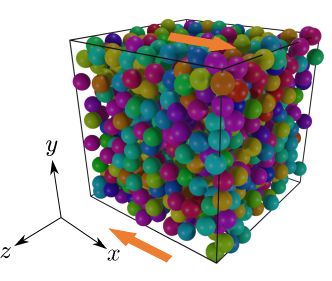
Figure 1: A snapshot of our system. Particles are initially distributed at random. The arrows indicate the shear direction.

Equation of motion of the suspended particle $i$ with its position $\bm{r}_{i}$ under a simple shear with the shear rate $\dot{\gamma}$ is given by

$$\frac{d\bm{p}_{i}}{dt}=\sum_{j\neq i}\bm{F}_{ij}-\zeta\bm{p}_{i}+\bm{\xi}_{i},$$ (2)

where $\bm{p}_{i}\equiv m\bm{V}_{i}$ with $\bm{V}_{i}\equiv\bm{v}_{i}-\dot{\gamma}y_{i}\hat{\bm{e}}_{x}$ with the unit vector $\hat{\bm{e}}_{x}$ parallel to $x$ direction and the velocity $\bm{v}_{i}$ of $i-$th particle is the peculiar momentum, $\bm{F}_{ij}\equiv-\partial U(r_{ij})/\partial\bm{r}_{ij}$ is the inter-particle force between $i$–th and $j$–th particles with $\bm{r}_{ij}\equiv\bm{r}_{i}-\bm{r}_{j}$ and $r_{ij}\equiv|\bm{r}_{ij}|$, and $T_{\mathrm{env}}$ is the environmental (solvent) temperature. Note that the drag coefficient $\zeta$ is expressed as $\zeta=3\pi\eta_{0}d/m$. The noise $\bm{\xi}_{i}(t)=\xi_{i,\alpha}(t)\hat{\bm{e}}_{\alpha}$ satisfies the fluctuation-dissipation relation:

$$\langle\bm{\xi}_{i}(t)\rangle=\bm{0},\quad\langle\xi_{i,\alpha}(t)\xi_{j,\beta}(t^{\prime})\rangle=2mT_{\mathrm{env}}\zeta\delta_{ij}\delta_{\alpha\beta}\delta(t-t^{\prime}),$$ (3)

where $\langle\cdot\rangle$ expresses the average over the noise.

The assumptions behind Eqs. (1), (2), and (3) are summarized as follows. (i) Suspended particles are monodisperse and frictionless. (ii) The inter-particle force is given by the harmonic potential in Eq. (1) and collisions between particles are elastic. (iii) Suspended particles are agitated by the white Gaussian noise as in Eq. (3). (iv) Suspended particles also feel Stokes’ drag while the hydrodynamic interaction between particles is ignored. (v) The environmental temperature $T_{\mathrm{env}}$ is independent of the motion of suspended particles. (vi) Perfect density matching between solvent and particles is assumed. Although aerosols cannot satisfy the density matching condition, the sedimentation is negligible within the observation time for small suspended particles [25, 26]. Note that the role of hydrodynamic interactions among particles in inertial suspensions is analyzed in another paper [45].

In the simulation, we also adopt the SLLOD dynamics [54, 53] to simulate the shear flow with the aid of the Lees-Edwards boundary condition [55] (see Fig. 1). As far as we have checked, the uniform flow is stable once the system reaches a steady state. The time increment for the simulations is chosen as $\Delta t=10^{-2}\min(d/\sqrt{2T/m},d\sqrt{m/\varepsilon})$, where $\min(a,b)$ chooses the smaller one between $a$ and $b$, which is small enough for the convergence of the results. In addition, all variables are nondimensionalized in terms of the mass $m$, the diameter $d$, and the drag coefficient $\zeta$. In the following, the control parameters are the volume fraction $\varphi$, the (dimensionless) shear rate $\dot{\gamma}^{*}$, the softness $\varepsilon^{*}$, and the strength of the noise $\xi_{\mathrm{env}}$. The explicit forms of these parameters are given by

$$\varphi\equiv\frac{\pi}{6}\frac{Nd^{3}}{L^{3}},\quad\dot{\gamma}^{*}\equiv\frac{\dot{\gamma}}{\zeta},\quad\varepsilon^{*}\equiv\frac{\varepsilon}{md^{2}\zeta^{2}},\quad\xi_{\mathrm{env}}\equiv\sqrt{\frac{T_{\mathrm{env}}}{m}}\frac{1}{d\zeta}.$$ (4)

Throughout this paper, we fix the number of particles as $N=1000$.

What we are interested in are the viscosity and kinetic temperature. The kinetic temperature $T$ and the viscosity $\eta$ are, respectively, defined by

$$T\equiv\frac{1}{N}\sum_{i}\frac{p_{i}^{2}}{3m},\quad\eta\equiv\frac{\sigma_{xy}}{\dot{\gamma}},$$ (5)

in the simulation. Here, the stress tensor $\sigma_{\alpha\beta}$ consists of two parts:

$$\sigma_{\alpha\beta}=\sigma_{\alpha\beta}^{k}+\sigma_{\mathrm{S},\alpha\beta}^{c},$$ (6)

where the kinetic and contact stresses, $\sigma_{\alpha\beta}^{k}$ and $\sigma_{\mathrm{S},\alpha\beta}^{c}$ are, respectively, given by

$$\sigma_{\alpha\beta}^{k}\equiv-\frac{1}{L^{3}}\sum_{i}\frac{p_{i,\alpha}p_{i,\beta}}{m},\quad\sigma_{\mathrm{S},\alpha\beta}^{c}\equiv-\frac{1}{L^{3}}\sum_{i}\sum_{j<i}r_{ij,\alpha}F_{ij,\beta}.$$ (7)

Here, the subscript S for $\sigma_{\mathrm{S},\alpha\beta}^{c}$ stands for the expression for soft-core systems. We can evaluate the dimensionless viscosity $\eta^{*}\equiv\eta\zeta/(nT_{\mathrm{env}})$ and dimensionless temperature $\theta$ from the simulation by

$$\eta^{*}\equiv\frac{\Pi_{xy}+\Pi_{\mathrm{S},xy}^{c}}{\dot{\gamma}^{*}},\quad\theta\equiv\frac{T}{T_{\mathrm{env}}},$$ (8)

where

$$\Pi_{\alpha\beta}\equiv\frac{\sigma_{\alpha\beta}^{k}}{nT_{\mathrm{env}}},\quad\Pi_{\mathrm{S},\alpha\beta}^{c}\equiv\frac{\sigma_{\mathrm{S},\alpha\beta}^{c}}{nT_{\mathrm{env}}}.$$ (9)

III Kinetic theory of inertial suspensions

In this section, we develop the kinetic theory of inertial suspensions consisting of frictionless soft particles. In the first subsection, we present the kinetic equation for the one-body distribution for the inertial suspension and present the moment equations for the stress tensor. Because the kinetic equation itself cannot be solved exactly, we put some assumptions in the subsequent subsections. In the second subsection, we adopt the Enskog approximation. In the third subsection, we employ Grad’s approximation to obtain a set of closure equations.

III.1 Kinetic equation for inertial suspensions

The kinetic theory is a powerful tool to describe the behavior of inertial suspensions quantitatively. The basic assumption of the kinetic theory is that both the random noise and collisions between particles are important, though the collisions have been ignored in the analysis of colloidal suspensions so far.

As shown in Appendices A.1 and A.2, the kinetic equation for the one-body distribution function $f(\bm{R}_{1},\bm{V}_{1};t)$ can be written as

$$\left[\frac{\partial}{\partial t}-\dot{\gamma}V_{1,y}\frac{\partial}{\partial V_{1,x}}+\bm{V}_{1}\cdot\frac{\partial}{\partial\bm{R}_{1}}\right]f(1)\approx\zeta\frac{\partial}{\partial\bm{V}_{1}}\cdot\left[\left(\bm{V}_{1}+\frac{T_{\mathrm{env}}}{m}\frac{\partial}{\partial\bm{V}_{1}}\right)f(1)\right]+J[\bm{V}_{1}|f^{(2)}(1,2)],$$ (10)

where $\bm{R}_{1}\equiv\bm{r}_{1}-\dot{\gamma}ty_{1}\hat{\bm{e}}_{x}$, $(1)$ and $(1,2)$ are the abbreviations of $(\bm{R}_{1},\bm{V}_{1};t)$ and $(\bm{R}_{1},\bm{V}_{1},\bm{R}_{2},\bm{V}_{2};t)$, respectively. To be consistent with the simulation setup, we ignore the hydrodynamic interaction between particles. If the interaction is short-ranged and collisions are elastic, $J[\bm{V}|f^{(2)}(1,2)]$ is given by [39]

$$J[\bm{V}_{1}|f^{(2)}(1,2)]=\int d\bm{V}_{2}\int d\bm{\Omega}\mathcal{S}(\chi,V_{12})V_{12}\left[f^{(2)}(1^{\prime\prime},2^{\prime\prime})-f^{(2)}(1,2)\right],$$ (11)

where $V_{12}\equiv|\bm{V}_{1}-\bm{V}_{2}|$, $(1^{\prime\prime},2^{\prime\prime})$ expresses a set of pre-collisional positions and velocities of $(1,2)$, $\chi$ is the scattering angle, $d\bm{\Omega}=\sin\chi d\chi d\phi$, and $\mathcal{S}(\chi,V)$ is the differential collision cross section (see also Fig. 2). Then, the particle trajectory is bent for $r_{\mathrm{min}}<r\leq d$ and is reflected at $r=r_{\mathrm{min}}$, where $r_{\mathrm{min}}$ is the turning point of the trajectory given by Eq. (82b), which depends on the impact parameter $b$ and the relative speed $v$ between two colliding particles. The explicit relationship between $\chi$ and the impact parameter $b$ is also presented in Appendix B. It is noted that the impact parameter $b$ is related to the differential cross section as $\mathcal{S}(\chi,V)\sin\chi=b|\partial b/\partial\chi|$ [56, 57].

As in the case of hard-core collisions, the relationships between the pre-collisional velocities $(\bm{V}_{1}^{\prime\prime},\bm{V}_{2}^{\prime\prime})$ and the post-collisional ones $(\bm{V}_{1},\bm{V}_{2})$ are expressed as

$$\begin{cases}\bm{V}_{1}^{\prime\prime}=\bm{V}_{1}-(\bm{V}_{12}\cdot\hat{\bm{k}}_{12})\hat{\bm{k}}_{12}\\ \bm{V}_{2}^{\prime\prime}=\bm{V}_{2}+(\bm{V}_{12}\cdot\hat{\bm{k}}_{12})\hat{\bm{k}}_{12}\end{cases},$$ (12)

where $\hat{\bm{k}}_{12}\equiv\bm{r}_{21}/r_{21}$. Note that $(\bm{V}_{1}^{\prime\prime},\bm{V}_{2}^{\prime\prime})$ and $(\bm{V}_{1},\bm{V}_{2})$ must be measured for $r>d$, i.e. without influence of the soft-core potential.

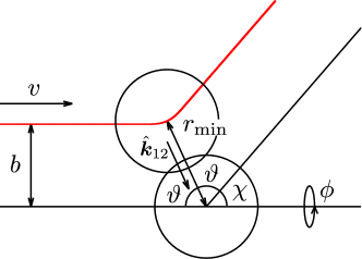
Figure 2: A schematic of a scattering process between two colliding particles with the impact parameter $b$ and the relative speed $v$, where the scattering angle $\chi$ and the closest distance $r_{\mathrm{min}}$ are given by Eqs. (82).

Now, let us assume that the system is uniform, and thus we can ignore the term $\bm{V}_{1}\cdot\partial f(\bm{R}_{1},\bm{V}_{1},t)/\partial\bm{R}_{1}$ in Eq. (10). Under this assumption, by multiplying $mV_{\alpha}V_{\beta}$ into Eq. (10) and integrating over $\bm{V}_{1}$, one obtains an approximate equation

$$\frac{d}{dt}\sigma_{\alpha\beta}^{k}+\dot{\gamma}\left(\delta_{\alpha x}\sigma_{y\beta}^{k}+\delta_{\beta x}\sigma_{y\alpha}^{k}\right)\approx-2\zeta\left(\sigma_{\alpha\beta}^{k}+nT_{\mathrm{env}}\delta_{\alpha\beta}\right)+\Lambda_{\alpha\beta},$$ (13)

where $\overleftrightarrow{\sigma^{k}}$ is the kinetic contribution of the stress tensor defined by

$$\overleftrightarrow{\sigma^{k}}\equiv-m\int d\bm{V}\bm{\mathrm{V}}\bm{\mathrm{V}}f(1),$$ (14)

and the collision moment by

$$\overleftrightarrow{\Lambda}\equiv-m\int d\bm{V}\bm{\mathrm{V}}\bm{\mathrm{V}}J[\bm{V}|f^{(2)}].$$ (15)

Let us introduce the theoretical temperature $T$ and two anisotropic temperatures $\Delta T$ and $\delta T$, respectively, as

$$T\equiv-\frac{\sigma^{k}_{\alpha\alpha}}{3n},\quad\Delta T\equiv-\frac{\sigma^{k}_{xx}-\sigma^{k}_{yy}}{n},\quad\delta T\equiv-\frac{\sigma^{k}_{xx}-\sigma^{k}_{zz}}{n},$$ (16)

where we have adopted Einstein’s convention in which double Greek characters take summation over $x$, $y$, and $z$, i.e. $\sigma^{k}_{\alpha\alpha}\equiv\sigma^{k}_{xx}+\sigma^{k}_{yy}+\sigma^{k}_{zz}$ throughout this paper. Then, Eq. (13) can be rewritten as

$$\frac{dT}{dt} =\frac{2}{3n}\dot{\gamma}\sigma^{k}_{xy}+2\zeta(T_{\mathrm{env}}-T)-\frac{1}{3n}\Lambda_{\alpha\alpha},$$ (17a)

$$\frac{d\Delta T}{dt} =\frac{2}{n}\dot{\gamma}\sigma^{k}_{xy}-2\zeta\Delta T-\frac{\delta\Lambda_{xx}-\delta\Lambda_{yy}}{n},$$ (17b)

$$\frac{d\delta T}{dt} =\frac{2}{n}\dot{\gamma}\sigma^{k}_{xy}-2\zeta\delta T-\frac{2\delta\Lambda_{xx}+\delta\Lambda_{yy}}{n},$$ (17c)

$$\frac{d\sigma^{k}_{xy}}{dt} =-\dot{\gamma}\sigma^{k}_{yy}-2\zeta\sigma^{k}_{xy}+\Lambda_{xy},$$ (17d)

where

$$\delta\Lambda_{xx}\equiv\Lambda_{xx}-\frac{1}{3}\Lambda_{\alpha\alpha},\quad\delta\Lambda_{yy}\equiv\Lambda_{yy}-\frac{1}{3}\Lambda_{\alpha\alpha}.$$ (18)

For practical calculations, let us rewrite the set of Eqs. (17) in the dimensionless forms. Let us introduce the dimensionless temperatures and kinetic deviatoric stress as

$$\Delta\theta\equiv\frac{\Delta T}{T_{\mathrm{env}}},\quad\delta\theta\equiv\frac{\delta T}{T_{\mathrm{env}}},\quad\Pi_{\alpha\beta}\equiv\frac{\sigma^{k}_{\alpha\beta}}{nT_{\mathrm{env}}}+\theta\delta_{\alpha\beta}$$ (19)

as well as the dimensionless time $\tau\equiv\dot{\gamma}t$. Using these quantities, the set of Eqs. (17) is rewritten as

$$\frac{d\theta}{d\tau} =\frac{2}{3}\dot{\gamma}^{*}\Pi_{xy}+2(1-\theta)-\frac{1}{3}\Lambda_{\alpha\alpha}^{*},$$ (20a)

$$\frac{d\Delta\theta}{d\tau} =2\dot{\gamma}^{*}\Pi_{xy}-2\Delta\theta-\delta\Lambda_{xx}^{*}+\delta\Lambda_{yy}^{*},$$ (20b)

$$\frac{d\delta\theta}{d\tau} =2\dot{\gamma}^{*}\Pi_{xy}-2\zeta\delta\theta-2\delta\Lambda_{xx}^{*}-\delta\Lambda_{yy}^{*},$$ (20c)

$$\frac{d\Pi_{xy}}{d\tau} =-\dot{\gamma}^{*}\Pi_{yy}-2\Pi_{xy}+\Lambda_{xy}^{*},$$ (20d)

with

$$\Lambda_{\alpha\beta}^{*}\equiv\frac{\Lambda_{\alpha\beta}}{n\zeta T_{\mathrm{env}}},\quad\delta\Lambda_{\alpha\beta}^{*}\equiv\frac{\delta\Lambda_{\alpha\beta}}{n\zeta T_{\mathrm{env}}}.$$ (21)

So far, we have not used any assumption in the framework of the kinetic theory for spatially uniform simple shear flows. However, this sef of equations (20) cannot be solved since it contains the two-body distribution $f^{(2)}(1,2)$. In the subsequent subsections, we adopt some assumptions to solve the set of equations (20).

III.2 Enskog approximation

In this subsection, we adopt the Enskog approximation to obtain a closure of the one-body distribution. It should be noted that the Enskog approximation is only applicable to hard-core systems because we cannot describe continuous changes in the distribution function for soft-core systems during contact in real soft-core situations. This problem does not appear in the Boltzmann equation for dilute gases because we do not need to consider the position dependence of the distribution function [56].

Instead of the analysis of real soft-core systems without approximation, we approximate a soft-core collision by a hard-core collision at the turning point $r=r_{\mathrm{min}}$ introduced in Eq. (82b). Therefore, the collision integral $J[\bm{V}|f^{(2)}(1,2)]$ can be approximated as

$$J[\bm{V}|f^{(2)}(1,2)]\simeq\int d\bm{V}_{2}\int d\bm{\Omega}\mathcal{S}(\chi,V_{12})V_{12}\left[f^{(2)}(\bm{R}_{1},\bm{V}_{1}^{\prime\prime},\bm{R}_{1}-r_{\mathrm{min}}\hat{\bm{k}}_{12},\bm{V}_{2}^{\prime\prime};t)-f^{(2)}(\bm{R}_{1},\bm{V}_{1},\bm{R}_{1}+r_{\mathrm{min}}\hat{\bm{k}}_{12},\bm{V}_{2};t)\right].$$ (22)

Within this approximation, the effect of softness is absorbed in the differential cross section $\mathcal{S}(\chi,V_{12})$.

Let us adopt the decoupling (Enskog) approximation of the two-body distribution function in which the two-body distribution function can be expressed as a product of the one-body distribution functions multiplied by the correlation function. Such a procedure is used for the Boltzmann equation for dilute gases and the Enskog equation for moderately dense gases [37, 29, 30, 32, 39, 40, 41, 42, 43, 44]. Since the collision is characterized by the turning point $r=r_{\mathrm{min}}$, we may utilize the decoupling approximation for hard-core particles as

$$f^{(2)}(1,2)\simeq g_{0}f(1)f(2),$$ (23)

where the radial distribution function at contact $g_{0}\equiv(1-\varphi/2)/(1-\varphi)^{3}$ is the dimensionless geometric factor to express the effect of the finite density [58]. Note that the volume fraction is not measured by the turning point but by the outer boundary of the acting potential force. It is also noted that the effect of shear on $g_{0}$ is ignored. In general, $g_{0}$ depends on the angle as discussed in Refs. [59, 60, 61]. The last assumption we use is

$$f\left(\bm{R}\mp r_{\mathrm{min}}\hat{\bm{k}}_{12},\bm{v}_{1};t\right)\simeq f\left(\bm{V}_{1}\pm\dot{\gamma}r_{\mathrm{min}}\hat{k}_{12,y}\hat{\bm{e}}_{x},t\right),$$ (24)

since we are interested in spatially uniform cases [36]. This assumption means that only affine deformations are considered. The validity of the above approximations can be verified by the comparison of the theoretical results with numerical results. Under these assumptions, the kinetic equation (10) is converted to the Enskog equation for the inertial suspension of frictionless soft-core particles [37, 29, 30, 32, 39, 40, 41, 42, 43, 44] as

$$\left(\frac{\partial}{\partial t}-\dot{\gamma}V_{1,y}\frac{\partial}{\partial V_{1,x}}\right)f(\bm{V}_{1},t)=\zeta\frac{\partial}{\partial\bm{V}_{1}}\cdot\left[\left(\bm{V}_{1}+\frac{T_{\mathrm{env}}}{m}\frac{\partial}{\partial\bm{V}_{1}}\right)f(1)\right]+J_{\mathrm{E}}[\bm{V}_{1}|f,f]$$ (25)

with

$$J_{\mathrm{E}}[\bm{V}_{1}|f,f]=g_{0}\int d\bm{V}_{2}\int d\Omega\mathcal{S}(\chi,V_{12})V_{12}\left[f\left(\bm{V}_{1}^{\prime\prime},t\right)f\left(\bm{V}_{2}^{\prime\prime}+\dot{\gamma}r_{\mathrm{min}}\hat{k}_{12,y}\hat{\bm{e}}_{x},t\right)-f\left(\bm{V}_{1},t\right)f\left(\bm{V}_{2}-\dot{\gamma}r_{\mathrm{min}}\hat{k}_{12,y}\hat{\bm{e}}_{x},t\right)\right],$$ (26)

where the subscript $\mathrm{E}$ is attached to represent the quantity under the Enskog approximation. Then, the collision moment (15) becomes [37]

$$\Lambda_{\alpha\beta}^{\mathrm{E}}=\overline{\Lambda}_{\alpha\beta}^{\mathrm{E}}-\dot{\gamma}(\delta_{\alpha x}\sigma^{c}_{\mathrm{H},y\beta}+\delta_{\beta x}\sigma^{c}_{\mathrm{H},y\alpha}),$$ (27)

where the quantity $\overline{\Lambda}^{\mathrm{E}}$ is defined by [37]

$$\overline{\Lambda}_{\alpha\beta}^{\mathrm{E}} \equiv\frac{m}{2}g_{0}\int d\bm{V}_{1}\int d\bm{V}_{2}\int d\Omega\mathcal{S}(\chi,V_{12})V_{12}(\bm{V}_{12}\cdot\hat{\bm{k}}_{12})$$

$$\hskip 10.00002pt\times\left[V_{12,\alpha}\hat{k}_{12,\beta}+V_{12,\beta}\hat{k}_{12,\alpha}-2(\bm{V}_{12}\cdot\hat{\bm{k}}_{12})\hat{k}_{12,\alpha}\hat{k}_{12,\beta})\right]f\left(\bm{V}_{1}+\dot{\gamma}r_{\mathrm{min}}\hat{k}_{12,y}\hat{\bm{e}}_{x},t\right)f\left(\bm{V}_{2},t\right).$$ (28)

Here, we adopt the approximation that the contact stress can be approximated by the collisional contribution to the stress of a hard-core system with the core diameter $r_{\mathrm{min}}$ as

$$\sigma_{\mathrm{H},\alpha\beta}^{c} \equiv-\frac{m}{2}g_{0}\int d\bm{V}_{1}\int d\bm{V}_{2}\int d\bm{\Omega}\mathcal{S}(\chi,V_{12})V_{12}r_{\mathrm{min}}(\bm{V}_{12}\cdot\hat{\bm{k}}_{12})\hat{k}_{12,\alpha}\hat{k}_{12,\beta}$$

$$\hskip 10.00002pt\times f\left(\bm{V}_{1}+\frac{1}{2}\dot{\gamma}r_{\mathrm{min}}\hat{k}_{12,y}\hat{\bm{e}}_{x},t\right)f\left(\bm{V}_{2}-\frac{1}{2}\dot{\gamma}r_{\mathrm{min}}\hat{k}_{12,y}\hat{\bm{e}}_{x},t\right),$$ (29)

where the subscript H stands for the expression for hard-core systems. Note that this $\sigma_{\mathrm{H},\alpha\beta}^{c}$ can be obtained once we know the one-body distribution function $f(\bm{V},t)$. Although the theoretical consistency between Eqs. (7) and (29) cannot be justified, we regard $\sigma_{\mathrm{S},\alpha\beta}^{c}$ as the correspondence of $\sigma_{\mathrm{H},\alpha\beta}^{c}$. This replacement sufficiently reproduces the simulation results as demonstrated in Appendix C.

When we analyze collision processes of soft-core particles, we need to consider the time dependence of differential cross section $\mathcal{S}(\chi,V_{12})$, which is too complicated to handle precisely. As previously mentioned in the previous subsection, the relationship between $b$ and $\chi=\pi-2\vartheta$ is given by $\mathcal{S}(\chi,V)\sin\chi=b|\partial b/\partial\chi|$. Using $d\hat{\bm{k}}_{12}=\sin\vartheta d\vartheta d\phi$ (see also Fig. 2) and that the distribution function may be independent of the angle $\phi$, one can get

$$\int d\Omega\mathcal{S}(\chi,V_{12})V_{12}=4\int d\vartheta d\phi\sin\vartheta\mathcal{S}(\chi,V_{12})V_{12}\cos\vartheta=4\int d\hat{\bm{k}}_{12}\mathcal{S}(\chi,V_{12})(V_{12}\cdot\hat{\bm{k}}_{12}).$$ (30)

Then, Eq. (28) can be rewritten as

$$\overline{\Lambda}_{\alpha\beta}^{\mathrm{E}} =4\times\frac{m}{2}g_{0}\int d\bm{V}_{1}\int d\bm{V}_{2}\int d\hat{\bm{k}}_{12}\mathcal{S}(\chi,V_{12})(\bm{V}_{12}\cdot\hat{\bm{k}}_{12})^{2}$$

$$\hskip 10.00002pt\times\left[V_{12,\alpha}\hat{k}_{12,\beta}+V_{12,\beta}\hat{k}_{12,\alpha}-2(\bm{V}_{12}\cdot\hat{\bm{k}}_{12})\hat{k}_{12,\alpha}\hat{k}_{12,\beta})\right]f\left(\bm{V}_{1}+\dot{\gamma}r_{\mathrm{min}}\hat{k}_{12,y}\hat{\bm{e}}_{x},t\right)f\left(\bm{V}_{2},t\right).$$ (31)

Since we ignore the continuous change of the distribution function during a contact, we can use

$$\mathcal{S}(\chi,V_{12})\simeq\frac{d^{2}}{4}\Omega_{2,2}^{*}\Theta(\bm{V}_{12}\cdot\hat{\bm{k}}_{12}),$$ (32)

where $\Omega_{2,2}^{*}$ is defined as [38, 56, 57]

$$\Omega_{k,\ell}^{*}\left(\frac{T}{\varepsilon}\right)\equiv\int_{0}^{\infty}dyy^{2\ell+3}e^{-y^{2}}\int_{0}^{1}db^{*}b^{*}\left[1-\sin^{k}\chi\left(b^{*},2y\sqrt{T^{*}}\right)\right]$$ (33)

with $b^{*}\equiv b/d$ and $T^{*}\equiv T/\varepsilon$. Note that $\Omega_{2,2}^{*}$ expresses the softness. The expression of Eq. (32) contains a decoupling approximation where we ignore the $\Omega$ dependence of the distribution function. Note that this $\Omega_{k,\ell}^{*}$ is independent of $\varphi$ [56, 57].

So far, the adopted approximations are reasonable, but it is still difficult to solve the Enskog equation because $r_{\mathrm{min}}$ depends on $b^{*}$ and $T^{*}$. Then, we adopt a crucial simplification for $r_{\mathrm{min}}$ by the replacement with $d$ as

$$r_{\mathrm{min}}\to d$$ (34)

for later discussion.

The temperature dependence of $\Omega_{2,2}^{*}$ is plotted in Fig. 3 as a theoretical result.

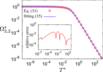
Figure 3: Temperature dependence of $\Omega_{2,2}^{*}$ given by Eq. (33) (open circles) and its fitting curve $\Omega_{2,2}^{\mathrm{fit}*}$ given by Eq. (35) (solid line). The inset shows the relative error $|\Omega_{2,2}^{*}-\Omega_{2,2}^{\mathrm{fit}*}|/\Omega_{2,2}^{*}$ against the temperature.

The softness parameter of the differential cross section $\Omega_{2,2}^{*}$ becomes $1$ in the low-temperature limit. This is because the kinetic energy is sufficiently smaller than the potential energy in this limit, which means that the trajectories of particles become almost the same as those of hard-core particles. $\Omega_{2,2}^{*}$ also behaves as $\Omega_{2,2}^{*}\sim(T/\varepsilon)^{-2}$ and $1-\Omega_{2,2}^{*}\sim(T/\varepsilon)^{1/2}$ in the high and low temperature regimes, respectively [38].

We also find that the temperature dependence of $\Omega_{2,2}^{*}$ can be well fitted by:

$$\Omega_{2,2}^{\mathrm{fit}*}(T^{*})=\frac{1}{1+a_{0}\sqrt{T^{*}}+a_{1}T^{*}+a_{2}T^{*2}},$$ (35)

with

$$a_{0}\simeq 2.6206,\quad a_{1}\simeq 0.39208,\quad a_{2}\simeq 154.37.$$ (36)

The relative error $|\Omega_{2,2}^{*}-\Omega_{2,2}^{\mathrm{fit}*}|/\Omega_{2,2}^{*}$ is smaller than $2\times 10^{-2}$ as shown in the inset of Fig. 3. Thus, it is sufficient to use Eq. (35) for the practical usage of $\Omega_{2,2}^{*}$.

After using the replacement (34), Eq. (31) is rewritten as

$$\overline{\Lambda}_{\alpha\beta}^{\mathrm{E}} =\frac{m}{2}d^{3}g_{0}\Omega_{2,2}^{*}\int d\bm{V}_{1}\int d\bm{V}_{2}\int d\hat{\bm{k}}_{12}\Theta(\bm{V}_{12}\cdot\hat{\bm{k}}_{12})(\bm{V}_{12}\cdot\hat{\bm{k}}_{12})^{2}$$

$$\hskip 10.00002pt\times\left[V_{12,\alpha}\hat{k}_{12,\beta}+V_{12,\beta}\hat{k}_{12,\alpha}-2(\bm{V}_{12}\cdot\hat{\bm{k}}_{12})\hat{k}_{12,\alpha}\hat{k}_{12,\beta})\right]f\left(\bm{V}_{1}+\dot{\gamma}d\hat{k}_{12,y}\hat{\bm{e}}_{x},t\right)f\left(\bm{V}_{2},t\right).$$ (37)

Substituting Eqs. (32)–(36) to Eq. (29), we obtain an approximate expression for the collisional contribution to the stress as

$$\sigma_{\mathrm{H},\alpha\beta}^{c} \simeq-\frac{m}{2}d^{3}g_{0}\Omega_{2,2}^{*}\int d\bm{V}_{1}\int d\bm{V}_{2}\int d\hat{\bm{k}}_{12}\Theta(\bm{V}_{12}\cdot\hat{\bm{k}}_{12})(\bm{V}_{12}\cdot\hat{\bm{k}}_{12})^{2}\hat{k}_{12,\alpha}\hat{k}_{12,\beta}$$

$$\hskip 10.00002pt\times f\left(\bm{V}_{1}+\frac{1}{2}\dot{\gamma}d\hat{k}_{12,y}\hat{\bm{e}}_{x},t\right)f\left(\bm{V}_{2}-\frac{1}{2}\dot{\gamma}d\hat{k}_{12,y}\hat{\bm{e}}_{x},t\right).$$ (38)

III.3 Rheology based on Grad’s approximation

Although we have adopted several assumptions to simplify the calculation in the previous subsection, it is still difficult to solve a set of equations (17) because the collision moment $\Lambda_{\alpha\beta}$ is an integral of a nonlinear function of $f(\bm{V},t)$. It is known that Grad’s approximation [62, 44, 63]

$$f(\bm{V},t)\simeq nv_{\mathrm{T}}^{-3}\tilde{f}_{\mathrm{M}}(\bm{c},t)\left(1-\frac{\Pi_{\alpha\beta}}{\theta}c_{\alpha}c_{\beta}\right)$$ (39)

with

$$\bm{c} \equiv\frac{\bm{V}}{v_{\mathrm{T}}},\quad v_{\mathrm{T}}\equiv\displaystyle\sqrt{\frac{2T}{m}},$$ (40)

and the dimensionless Maxwell distribution

$$\tilde{f}_{\mathrm{M}}(\bm{c},t)=\pi^{-3/2}\exp\left(-c^{2}\right),$$ (41)

yields good approximations for hard-core [27, 36, 42, 44, 64, 65, 37, 72, 71, 68, 69, 70, 66, 67] and dilute soft-core [38, 73] systems. An extended Grad’s approximation is also used for non-Brownian suspensions, in which $\Pi_{\alpha\beta}$ is replaced with the counterpart of the contact stress [60]. We adopt Grad’s approximation for moderately dense inertial suspensions consisting of soft-core particles in this paper.

We follow the parallel procedure to those used in Refs. [37, 75, 74], where the collisional moment and the contact stress are written in a series of an expansion parameter given by

$$\tilde{\dot{\gamma}}\equiv\frac{\dot{\gamma}^{*}}{\xi_{\mathrm{env}}\sqrt{\theta}}.$$ (42)

Thus, the corresponding terms in Eq. (21) are, respectively, given by

$$\Lambda_{\alpha\alpha}^{*} \simeq\varphi g_{0}\xi_{\mathrm{env}}\theta^{3/2}\Omega_{2,2}^{*}\sum_{i=0}^{N_{\mathrm{c}}}C_{1}^{(i)}\tilde{\dot{\gamma}}^{i},\quad\Lambda_{xy}^{*}\simeq\varphi g_{0}\xi_{\mathrm{env}}\theta^{3/2}\Omega_{2,2}^{*}\sum_{i=0}^{N_{\mathrm{c}}}C_{2}^{(i)}\tilde{\dot{\gamma}}^{i},$$ (43a)

$$\delta\Lambda_{xx}^{*} \simeq\varphi g_{0}\xi_{\mathrm{env}}\theta^{3/2}\Omega_{2,2}^{*}\sum_{i=0}^{N_{\mathrm{c}}}C_{3}^{(i)}\tilde{\dot{\gamma}}^{i},\quad\delta\Lambda_{yy}^{*}\simeq\varphi g_{0}\xi_{\mathrm{env}}\theta^{3/2}\Omega_{2,2}^{*}\sum_{i=0}^{N_{\mathrm{c}}}C_{4}^{(i)}\tilde{\dot{\gamma}}^{i}.$$ (43b)

Strictly speaking, we should set $N_{\mathrm{c}}\to\infty$ in Eqs. (43). This treatment with $N_{\mathrm{c}}\to\infty$ has been performed for sheared dry granular gases with hard-core particles [76], but nobody has succeeded for our setup. However, it is sufficient to terminate the calculation at a finite order $N_{\mathrm{c}}$ for practical use. This is because the convergence is fast enough when the collisions are elastic (see Appendix D). In this paper, we adopt $N_{\mathrm{c}}=2$.

After putting some assumptions explained in the previous subsections, we can rewrite the set of (dimensionless) dynamic equations (20). We note that the coefficients $C_{1}^{(i)}$, $C_{2}^{(i)}$, $C_{3}^{(i)}$, and $C_{4}^{(i)}$ in Eqs. (43) can be written in terms of these dimensionless quantities [37, 75, 74]. Then, with the aid of Eqs. (43), the set of (dimensionless) dynamic equations (20) is rewritten as

$$\frac{d\theta}{d\tau} =\frac{2}{3}\dot{\gamma}^{*}\Pi_{xy}+2(1-\theta)-\frac{1}{3}\varphi g_{0}\xi_{\mathrm{env}}\theta^{3/2}\Omega_{2,2}^{*}\sum_{i=0}^{N_{\mathrm{c}}}C_{1}^{(i)}\tilde{\dot{\gamma}}^{i},$$ (44a)

$$\frac{d\Delta\theta}{d\tau} =2\dot{\gamma}^{*}\Pi_{xy}-2\Delta\theta-\varphi g_{0}\xi_{\mathrm{env}}\theta^{3/2}\Omega_{2,2}^{*}\sum_{i=0}^{N_{\mathrm{c}}}\left(C_{3}^{(i)}-C_{4}^{(i)}\right)\tilde{\dot{\gamma}}^{i},$$ (44b)

$$\frac{d\delta\theta}{d\tau} =2\dot{\gamma}^{*}\Pi_{xy}-2\delta\theta-\varphi g_{0}\xi_{\mathrm{env}}\theta^{3/2}\Omega_{2,2}^{*}\sum_{i=0}^{N_{\mathrm{c}}}\left(2C_{3}^{(i)}+C_{4}^{(i)}\right)\tilde{\dot{\gamma}}^{i},$$ (44c)

$$\frac{d\Pi_{xy}}{d\tau} =\dot{\gamma}^{*}\left(\theta-\frac{2}{3}\Delta\theta+\frac{1}{3}\delta\theta\right)-2\Pi_{xy}+\varphi g_{0}\xi_{\mathrm{env}}\theta^{3/2}\Omega_{2,2}^{*}\sum_{i=0}^{N_{\mathrm{c}}}C_{2}^{(i)}\tilde{\dot{\gamma}}^{i}.$$ (44d)

We can solve the set of equations (44) numerically to obtain $\theta$, $\Delta\theta$, $\delta\theta$, and $\Pi_{xy}$. Substituting them into Eq. (39) we can obtain the approximate velocity distribution function. Then, inserting this distribution function into Eq. (38) we can determine the collisional contribution to the stress as a series of $\tilde{\dot{\gamma}}$ as

$$\sigma_{\mathrm{H},xy}^{c}\simeq\frac{\pi}{6}n^{2}d^{3}g_{0}T\Omega_{2,2}^{*}\sum_{i=0}^{N_{\mathrm{c}}}C_{5}^{(i)}\tilde{\dot{\gamma}}^{i}.$$ (45)

Therefore, we obtain the approximate expression of the (dimensionless) viscosity as

$$\eta^{*}\simeq\frac{\Pi_{xy}+\Pi_{\mathrm{H},xy}^{c}}{\dot{\gamma}^{*}},$$ (46)

with

$$\Pi_{\mathrm{H},xy}^{c}\equiv\frac{\sigma_{\mathrm{H},xy}^{c}}{nT_{\mathrm{env}}}.$$ (47)

To close this section, we list the assumptions used in the theoretical analysis. (i) We ignore the spatial inhomogeneity in the simple shear flow. (ii) We adopt the Enskog approximation even for soft-core systems, in which we regard the turning diameter $r_{\mathrm{min}}$ as the impact-speed dependent inner-hard core. Then, the contact stress for the soft-core system is approximated by that for the hard-core system in Eq. (29), which is evaluated by the product of the one-body distribution function. (iii) Using the decoupling approximation, the differential cross section is reduced to $\Omega_{2,2}^{*}d^{2}/4$ as in Eq. (32). To evaluate $\Omega_{2.2}^{*}$ we adopt a Padé approximation as in Eq. (35). (iv) We replace $r_{\mathrm{min}}$ with $d$ after we extract $\Omega_{2,2}^{*}$ which expresses the soft-core effect. This is the most crucial approximation. (v) We adopt Grad’s approximation Eq. (39). We note that assumptions (i) and (v) are commonly used even for the dilute system [38], while the other assumptions (ii)–(iv) are newly introduced for moderately dense systems in this paper.

IV Steady rheology

In this section, we present the theoretical predictions of steady rheology based on the solutions of a set of dynamic equations (44) and compare the results with those by the simulation. As already mentioned, we adopt $N_{\mathrm{c}}=2$ for the analysis in Eqs. (43) and (45). Although the results of the linear theory with $N_{\mathrm{c}}=1$ are a little deviated from those of $N_{\mathrm{c}}\geq 2$, there are some analytic expressions in the linear theory as in Appendix D.2.

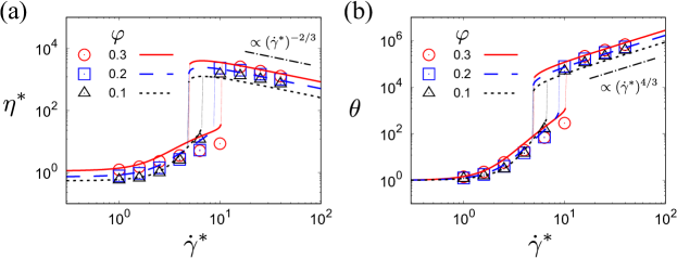
Figure 4: Plots of the theoretical (a) $\eta^{*}$ and (b) $\theta$ against $\dot{\gamma}^{*}$ for $\varphi=0.10$ (dotted line), $0.20$ (dashed line), and $0.30$ (solid line) with fixing $\xi_{\mathrm{env}}=1.0$, $\varepsilon^{*}=10^{4}$, and $N_{\mathrm{c}}=2$, where the theoretical curves are obtained by Eqs. (44)–(47). The left and the right vertical dotted lines are discontinuous changes of $\eta^{*}$ and $\theta$ from the ignited and the quenched phases, respectively. The symbols for circles ($\varphi=0.3$), squares ($\varphi=0.20$), and triangles ($\varphi=0.1$) correspond to the simulation results. The guide lines represent $\eta^{*}\propto(\dot{\gamma}^{*})^{-2/3}$ and $\theta\propto(\dot{\gamma}^{*})^{4/3}$, respectively.

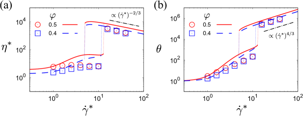
Figure 5: Plots of the theoretical (a) $\eta^{*}$ and (b) $\theta$ against $\dot{\gamma}^{*}$ for $\varphi=0.40$ (dotted line) and $0.50$ (dashed line) with fixing $\xi_{\mathrm{env}}=1.0$, $\varepsilon^{*}=10^{4}$, and $N_{\mathrm{c}}=2$, where the theoretical curves are obtained by Eqs. (44)–(47). The left and the right vertical dotted lines are discontinuous changes of $\eta^{*}$ and $\theta$ from the ignited and the quenched phases, respectively. The symbols for circles ($\varphi=0.50$) and squares ($\varphi=0.40$) correspond to the simulation results. The guide lines represent $\eta^{*}\propto(\dot{\gamma}^{*})^{-2/3}$ and $\theta\propto(\dot{\gamma}^{*})^{4/3}$, respectively.

Figures 4 and 5 show the comparison of the theory of $N_{\mathrm{c}}=2$ for $\eta^{*}$ and $\theta$ versus $\dot{\gamma}^{*}$ with the results of the simulation for $\varphi=0.10$, $0.20$, and $0.30$ in Fig. 4, and $0.40$ and $0.50$ in Fig. 5, respectively, with fixing $\varepsilon^{*}=10^{4}$, and $\xi_{\mathrm{env}}=1.0$. Now, the theoretical values of $\eta^{*}$ and $\theta$ are obtained by solving the set of Eqs. (44) with the aid of Eqs. (43) and (46). We have numerically solved the set of equations (44) under the initial kinetic temperature $\theta=1$ at $\tau=0$. As can be seen in these figures, the theory gives reasonable agreement with the results of simulations even for $\varphi=0.50$, though the agreement between the theory and simulation for large $\varphi$ is a little worse than that in the dilute case. It should be noted that all theoretical flow curves having DST-like ignited-quenched transitions are associated with hysteresis. For later discussion, we simply call the DST-like ignited-quenched transition the DST or DST-like change.

Remarkably, the DST can be observed in the wide range of $\varphi$ from the dilute limit [38] to $\varphi=0.50$, as shown in Figs. 4 and 5. These results differ from the conventional DST which can be only observed in dense colloidal suspensions [1, 2, 3, 4, 52]. These discontinuous changes of $\eta^{*}$ and $\theta$ in the wide range of $\varphi$ are also different from those of hard-core inertial suspensions, where the DST becomes the CST above a critical fraction which is a few percent [29, 33, 27, 36, 37]. Our results indicate that the DST observed here is induced by the softness and the inertial effect of particles. In addition, the system exhibits shear thinning for $\dot{\gamma}^{*}\gg 1$. As reported in Ref. [38], $\Omega_{2,2}^{*}$ behaves as $\Omega_{2,2}^{*}\sim\theta^{-2}$ for $\dot{\gamma}^{*}\gg 1$. As a result, the viscosity and temperature should behave as $\eta^{*}\sim(\dot{\gamma}^{*})^{-2/3}$ and $\theta\sim(\dot{\gamma}^{*})^{4/3}$ for $\dot{\gamma}^{*}\gg 1$. These theoretical predictions are consistent with those obtained from the simulations as shown in Figs. 4 and 5. Thus, our crucial assumption in Eq. (34) does not cause any significant disagreement between the theory and simulation.

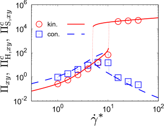
Figure 6: Plots of the theoretical kinetic shear stress $\Pi_{xy}$ (red solid line) and contact shear stress $\Pi_{\mathrm{H},xy}^{c}$ (blue dashed line) against $\dot{\gamma}^{*}$ for $\varphi=0.30$ with fixing $\xi_{\mathrm{env}}=1.0$, $\varepsilon^{*}=10^{4}$, and $N_{\mathrm{c}}=2$, where the theoretical curves are obtained by Eqs. (44)–(47). The symbols (circles for the kinetic stress and squares for the contact stress $\Pi_{\mathrm{S},xy}^{c}$) correspond to the simulation results. The left and the right vertical dotted lines are discontinuous changes of the shear stress from the ignited and the quenched phases, respectively.

Interestingly, the contact stress $\Pi_{xy}^{c}$ decreases as $\dot{\gamma}^{*}$ increases for $\dot{\gamma}>\dot{\gamma}_{\mathrm{c}}$, while the kinetic stress abruptly increases around $\dot{\gamma}=\dot{\gamma}_{\mathrm{c}}$ as shown in Fig. 6. This is because the duration time becomes negligibly small when the kinetic temperature becomes sufficiently large [38]. Thus, the DST can be observed only when we consider the kinetic stress. Our result is consistent with Kawasaki et al. [50] which presented only the contact stress.

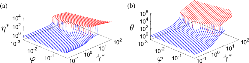
Figure 7: The theoretical flow curves for (a) $\eta^{*}$ and (b) $\theta$ against $\varphi$ and $\dot{\gamma}^{*}$ for $\xi_{\mathrm{env}}=1.0$ and $\varepsilon^{*}=10^{4}$, respectively, where the theoretical curves are obtained by Eqs. (44)–(47). Here, the red and the blue solid lines express the flow curves in the ignited and quenched phases, respectively, and the red and blue dotted lines are discontinuous changes of $\eta^{*}$ and $\theta$ from the ignited and quenched phases, respectively.

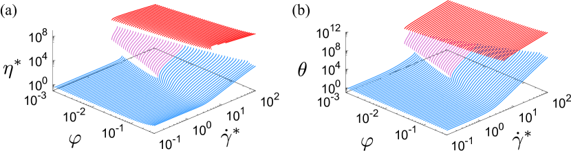
Figure 8: The theoretical flow curves for (a) $\eta^{*}$ and (b) $\theta$ against $\varphi$ and $\dot{\gamma}^{*}$ for $\xi_{\mathrm{env}}=1.0$ and $\varepsilon^{*}=10^{8}$, respectively, where the theoretical curves are obtained by Eqs. (44)–(47). Here, the red and the blue lines express the flow curves in the ignited and the quenched phases, respectively, while the purple lines represent the intermediate thickening phase that appears only for $\varphi<1.8\times 10^{-2}$.

Figures 7 and 8 also exhibit how the DST-like transitions of $\eta^{*}$ and $\theta$ depend on $\varphi$ and $\dot{\gamma}^{*}$ for $\varepsilon^{*}=10^{4}$ and $10^{8}$, respectively, with fixing $\xi_{\mathrm{env}}=1.0$ based on the kinetic theory with $N_{\mathrm{c}}=2$. As indicated by Ref. [38], there are two-step DST-like changes of $\eta^{*}$ and $\theta$ at $\dot{\gamma}^{*}_{\mathrm{c}1}$ and $\dot{\gamma}_{\mathrm{c}}^{*}$ for dilute inertial suspensions. The DST-like changes at $\dot{\gamma}_{\mathrm{c}1}^{*}$ disappear for $\varphi>\varphi_{\mathrm{c}_{1}}\simeq 0.01$, corresponding to the disappearance of the DST-like behavior in hard-core systems [33, 36]. On the other hand, the DST-like changes of $\eta^{*}$ and $\theta$ at $\dot{\gamma}^{*}_{\mathrm{c}}$ survive in the wide range of $\varphi$ for larger $\varepsilon^{*}$ (see Fig. 8).

These results are counterintuitive, but as shown in Fig. 9, $\eta^{*}$ can be scaled by $\epsilon^{*4/3}$ in the vicinity of $\dot{\gamma}_{\mathrm{c}}^{*}$ except for extremely soft particles (such as $\varepsilon^{*}=1$). This means that the viscosity in the ignited phase diverges in the hard-core limit. Thus, we can only observe the CST for moderately dense inertial suspensions consisting of hard-core particles.

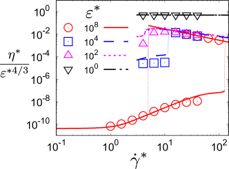
Figure 9: Plots of $\eta^{*}/\varepsilon^{*4/3}$ against $\dot{\gamma}^{*}$ for various $\varepsilon^{*}$ with fixing $\varphi=0.40$ and $\xi_{\mathrm{env}}=1.0$. The theoretical results are expressed as lines (red solid lines for $\varepsilon^{*}=10^{8}$, blue dashed line for $\varepsilon^{*}=10^{4}$, purple dotted line for $\varepsilon^{*}=10^{2}$, and black chain line for $\varepsilon^{*}=1$), where the theoretical curves are obtained by Eqs. (44)–(47). The symbols (circles for $\varepsilon^{*}=10^{8}$, squares for $\varepsilon^{*}=10^{4}$, purple upper triangles for $\varepsilon^{*}=10^{2}$ and black lower triangles for $\varepsilon^{*}=1$) are obtained by the simulation. The left and the right vertical dotted lines are discontinuous changes of $\eta^{*}$ from the ignited and the quenched phases, respectively.

We also check how the rheology depends on the softness parameter $\varepsilon^{*}$. Figure 10 exhibits the comparison of the theoretical results with those of the simulations for $\varepsilon^{*}=10^{0}$, $10^{2}$, $10^{4}$, and $10^{6}$ with fixed $\varphi=0.40$ and $\xi_{\mathrm{env}}=1.0$. As can be seen in Fig. 10, the theory gives reasonable agreement with the results of simulations. Figure 10 also indicates that the DST-like discontinuous changes of $\eta^{*}$ and $\theta$ of moderately dense inertial suspensions disappear, at least, for $\varepsilon^{*}\leq 10$.

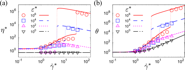
Figure 10: Plots of (a) $\eta^{*}$ and (b) $\theta$ against $\dot{\gamma}^{*}$ for $\varepsilon^{*}=1,10^{2},10^{4}$, and $10^{6}$ with fixed $\varphi=0.40$ and $\xi_{\mathrm{env}}=1.0$. Here, the lines express the theoretical flow curves with $N_{\mathrm{c}}=2$ obtained by Eqs. (44)–(47). The corresponding symbols are obtained by the simulation. The left and the right vertical dotted lines are discontinuous changes of $\eta^{*}$ and $\theta$ from the ignited and the quenched phases, respectively.

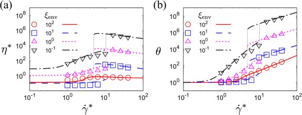
Figure 11: Plots of (a) $\eta^{*}$ and (b) $\theta$ against $\dot{\gamma}^{*}$ for $\xi_{\mathrm{env}}=10^{-1}$, $10^{0}$, $10^{1}$, and $10^{2}$ when we fix $\varphi=0.30$ and $\varepsilon^{*}=10^{4}$. Here, the lines express the theoretical expressions, where the theory is given by Eqs. (44)–(47). The corresponding symbols are obtained by the simulation. The left and the right vertical dotted lines are discontinuous changes of $\eta^{*}$ and $\theta$ from the ignited and the quenched phases, respectively.

Next, let us also investigate $\xi_{\mathrm{env}}$ dependence of the flow curves. Figure 11 demonstrates that the theory works well in the wide range of $\xi_{\mathrm{env}}$ when we fix $\varphi=0.30$ and $\varepsilon^{*}=10^{4}$. The DST-like changes of $\eta^{*}$ and $\theta$ disappear if $\xi_{\mathrm{env}}$ is large enough such as $\xi_{\mathrm{env}}=10^{2}$. To clarify the critical $\xi_{\rm env}$, we control $\xi_{\rm env}$ in the range $60\leq\xi_{\rm env}\leq 70$ with fixing $\varphi=0.30$ and $\varepsilon^{*}=10^{4}$. As shown in Fig. 12, the divergence of the slope $d\eta^{*}/d\dot{\gamma}^{*}$ disappears at around $\xi_{\mathrm{env}}\simeq 66$. This means that there is a transition from DST to CST at this point.

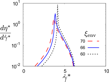
Figure 12: Plots of $d\eta^{*}/d\dot{\gamma}^{*}$ against $\dot{\gamma}^{*}$ obtained from the theory for $\xi_{\mathrm{env}}=60$, $66$, and $70$ when we fix $\varphi=0.30$ and $\varepsilon^{*}=10^{4}$.

Figures 13 presents the results of the simulation to show how $\eta^{*}$ and $\theta$ depend on $\varepsilon^{*}$ and $\dot{\gamma}^{*}$ for $\varphi=0.4$ and $\xi_{\mathrm{env}}=1.0$. These figures indicate that both $\eta^{*}$ and $\theta$ are continuous for small $\varepsilon^{*}$ but become discontinuous if $\varepsilon^{*}$ is larger than a critical value. Similarly, Fig. 14 illustrates how $\eta^{*}$ and $\theta$ depend on $\dot{\gamma}^{*}$ and $\xi_{\mathrm{env}}$ for $\varphi=0.40$ and $\varepsilon^{*}=10^{4}$. These figures indicate that the discontinuous changes of $\eta^{*}$ and $\theta$ become continuous if $\xi_{\mathrm{env}}$ is larger than a critical value.

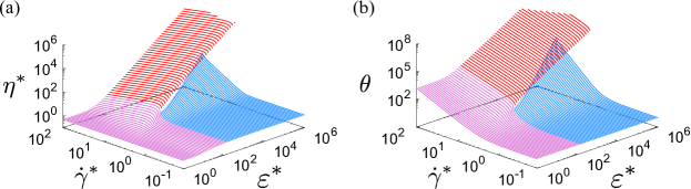
Figure 13: Plots of the theoretical (a) $\eta^{*}$ and (b) $\theta$ against $\dot{\gamma}^{*}$ and $\varepsilon^{*}$ when we fix $\varphi=0.30$ and $\xi_{\mathrm{env}}=1.0$, where the theoretical curves are drawn based on Eqs. (44)–(47). The red and the blue lines express the flow curves in the ignited and the quenched phases, respectively, while the purple lines represent the flow curves for the continuous shear thickening.

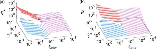
Figure 14: Plots of the theoretical (a) $\eta^{*}$ and (b) $\theta$ against $\dot{\gamma}^{*}$ and $\xi_{\mathrm{env}}$ when we fix $\varphi=0.30$ and $\varepsilon^{*}=10^{4}$, where the theoretical curves are drawn based on Eqs. (44)–(47). The red and the blue lines express the flow curves in the ignited and the quenched phases, respectively, while the purple lines represent the flow curves for the continuous shear thickening.

Finally, we comment on the validity of the theoretical assumptions (i)–(v) listed in the last paragraph of the previous section. Although we cannot obtain the explicit expression of $\Lambda_{\alpha\beta}$ in moderately dense suspensions, we can write its form explicitly in the dilute limit with the assumptions (i) and (v) (see Appendix E). This leads to the precise results as shown in Ref. [38]. The additional assumptions used in (ii)–(iv) which cannot be justified lead to slight deviations of the theoretical predictions from the simulation results. Nevertheless, it is unexpected that our theoretical results reasonably agree with the simulation results.

V Concluding remarks

This study successfully demonstrates the existence of DST-like changes in the viscosity and kinetic temperature in moderately dense inertial suspensions comprising frictionless soft-core particles using Langevin simulation. By adopting several assumptions in the theoretical analysis, the kinetic theory well describes the discontinuous changes of both the viscosity and the kinetic temperature in the wide range of parameters’ space if we ignore the hydrodynamic interactions among particles. Notably, our findings have confirmed that these discontinuous changes persist even when considering hydrodynamic interactions between particles as illustrated in Ref. [45]. We also stress that the recent MD simulation for a mixture supports the validity of the kinetic theory without hydrodynamic interactions [46]. This unveils a new mechanism for DST caused by the ignited-quenched transition for frictionless soft-core particles.

It is hard to observe the discontinuous changes of $\eta^{*}$ and $\theta$ obtained in our model experimentally if the solvent is a liquid. The significant increase in kinetic temperature during the ignited phase, possibly reaching $10^{6}$ times that of the quenched phase, might lead to liquid evaporation due to intense stirring effects caused by suspended particles. Our model does not encompass the heat-up of $T_{\mathrm{env}}$ due to stirring effects. Even if we consider particles suspended in a gas, it might be difficult to be free from the melting of solid particles. Nevertheless, the indication of the existence of DST-like changes of $\eta^{*}$ and $\theta$ for frictionless soft-core particles even for relatively dense suspensions is important.

Let us discuss the possibility of experimental observation when we consider aerosols. Here, let us assume that the diameter, the mass density, and Young’s modulus $Y$ of aerosol particles are roughly given by $d\sim 10^{-6}\ \mathrm{m}$, $\rho\sim 1\ \mathrm{g/cm^{3}}$, and $Y\sim 10\ \mathrm{GPa}$, and thus, the mass becomes $m\sim 10^{-14}\ \mathrm{kg}$. When we consider a case when the solvent is air, whose viscosity is approximately $\eta_{0}\sim 10^{-5}\ \mathrm{Pa\cdot s}$. The corresponding drag coefficient becomes $\zeta=3\pi\eta_{0}d/m\sim 10^{4}\ 1/\mathrm{s}$. Because the DST takes place at around $\dot{\gamma}\sim\zeta\sim 10^{4}\ 1/\mathrm{s}$, this corresponds to the shear rate $\dot{\gamma}\sim 10^{4}\ \mathrm{1/s}$.

As indicated in Ref. [45] the used value of $\xi_{\rm env}$ (order of unity) is too large if we compare them with the typical value $\sim 10^{-4}$ for colloidal suspensions in experiments. Nevertheless, the kinetic theory predicts the existence of the DST even for $\xi_{\rm env}=10^{-4}$ as shown in Fig. 15. Note that the DST in our model can be observed for $\xi_{\mathrm{env}}<\xi_{\mathrm{env}}^{\mathrm{c}}\approx 66$ as shown in Fig. 14. This suggests that we can expect the experimental observation of the DST even for frictionless grains.

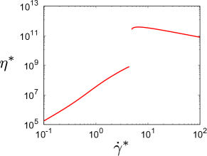
Figure 15: Plot of $\eta^{*}$ against $\dot{\gamma}^{*}$ for $\xi_{\mathrm{env}}=10^{-4}$ obtained by Eqs. (44)–(47) with fixed $\varphi=0.30$ and $\varepsilon^{*}=10^{4}$.

Needless to say, it is important to analyze suspensions of frictional grains corresponding to the typical experimental setup for colloidal suspensions. This subject would be our future task.

Appendix A The basis of the kinetic theory of inertial suspension of soft particles

In this appendix, we explain the basis of the kinetic theory. The appendix consists of two parts. In the first subsection, we explain the framework of the kinetic theory. In the second subsection, we derive the kinetic equation of the inertial suspension of soft particles.

A.1 Framework of kinetic model

Let us consider an $N$-body distribution function $f^{(N)}(\{\bm{r}_{i}\},\{\bm{p}_{i}\},t)$. We adopt the abbreviation $f^{(N)}\equiv f^{(N)}(\{\bm{r}_{i}\},\{\bm{p}_{i}\},t)$ to simplify the notation. From the conservation of probability, one gets [39, 77, 78, 53]

$$\frac{\partial f^{(N)}}{\partial t}+\sum_{i}\frac{\partial}{\partial\bm{r}_{i}}\cdot\left(\frac{d\bm{r}_{i}}{dt}f^{(N)}\right)+\sum_{i}\frac{\partial}{\partial\bm{p}_{i}}\cdot\left(\frac{d\bm{p}_{i}}{dt}f^{(N)}\right)=0$$ (48)

for soft particles. Substituting Eq. (2) into Eq. (48), we obtain the stochastic-Liouville equation

$$\frac{\partial f^{(N)}}{\partial t}+\sum_{i}\frac{\partial}{\partial\bm{r}_{i}}\cdot\left[\left(\frac{\bm{p}_{i}}{m}+\dot{\gamma}y_{i}\hat{\bm{e}}_{x}\right)f^{(N)}\right]+\sum_{i}\frac{\partial}{\partial\bm{p}_{i}}\cdot\left[\left(\sum_{j\neq i}\bm{F}_{ij}-\zeta\bm{p}_{i}+\bm{\xi}_{i}\right)f^{(N)}\right]=0.$$ (49)

With the aid of the noise average, Eq. (49) can be rewritten as

$$\left[\frac{\partial}{\partial t}+\sum_{i}\bm{V}_{i}\cdot\frac{\partial}{\partial\bm{r}_{i}}-\sum_{i}\dot{\gamma}V_{i,y}\frac{\partial}{\partial V_{i,x}}\right]\langle f^{(N)}\rangle=\sum_{i}\frac{\partial}{\partial\bm{V}_{i}}\cdot\left[\zeta\left(\bm{V}_{i}+\frac{T_{\mathrm{env}}}{m}\frac{\partial}{\partial\bm{V}_{i}}\right)\langle f^{(N)}\rangle\right]-\sum_{i,j}\frac{\partial}{\partial\bm{V}_{i}}\cdot\left(\frac{\bm{F}_{ij}}{m}\langle f^{(N)}\rangle\right),$$ (50)

where $\langle f^{(N)}\rangle$ is the noise-averaged distribution function and we have introduced $\bm{V}_{i}\equiv\bm{p}_{i}/m$. Integrating Eq. (50) over $\bm{r}_{i}$ and $\bm{V}_{i}$ for $i=2,3,\cdots,N$, we obtain

$$\left[\frac{\partial}{\partial t}+\bm{V}_{1}\cdot\frac{\partial}{\partial\bm{r}_{1}}-\dot{\gamma}V_{1,y}\frac{\partial}{\partial V_{1,x}}\right]f(X_{1};t)$$

$$=\frac{\partial}{\partial\bm{V}_{1}}\cdot\left[\zeta\left(\bm{V}_{1}+\frac{T_{\mathrm{env}}}{m}\frac{\partial}{\partial\bm{V}_{1}}\right)f(X_{1};t)\right]-\frac{1}{N-1}\sum_{j}\frac{\partial}{\partial\bm{V}_{1}}\cdot\left(\frac{\bm{F}_{1j}}{m}f^{(2)}(X_{1},X_{j};t)\right)$$

$$\simeq\frac{\partial}{\partial\bm{V}_{1}}\cdot\left[\zeta\left(\bm{V}_{1}+\frac{T_{\mathrm{env}}}{m}\frac{\partial}{\partial\bm{V}_{1}}\right)f(X_{1};t)\right]-\frac{\partial}{\partial\bm{V}_{1}}\cdot\left(\frac{\bm{F}_{12}}{m}f^{(2)}(X_{1},X_{2};t)\right),$$ (51)

where we have introduced one- and two-body distribution functions as

$$f(X_{1};t) \equiv\frac{1}{(N-1)!(L^{3})^{N-1}}\int\prod_{j=2}^{N}dX_{j}\langle f^{(N)}\rangle,$$ (52a)

$$f^{(2)}(X_{1},X_{2};t) \equiv\frac{1}{(N-2)!(L^{3})^{N-2}}\int\prod_{j=3}^{N}dX_{j}\langle f^{(N)}\rangle$$ (52b)

with $dX_{j}\equiv d\bm{r}_{j}d\bm{p}_{j}$, and $X_{j}\equiv(\bm{r}_{j},\bm{p}_{j})$. To obtain the last expression in Eq. (51), we put $j=2$ and attach $N-1$ factor to the second and third terms on the right-hand side (RHS) of Eq. (51) in the first line. As shown in Appendix A.2 the last term on the RHS of Eq. (51) can be written as the collision integral $J[\bm{V}_{1}|f^{(2)}(1,2)]$, at least, in the low density limit. Thus, we can reach Eq. (10).

A.2 Derivation of the equation of one-body distribution function

In this subsection, we derive the collision operator for a dilute gas without solvents based on Ref. [77].

The stochastic Liouville equation can be rewritten as

$$\frac{\partial f^{(N)}}{\partial t}=(\mathcal{L}^{(N)}+\mathcal{L}_{\dot{\gamma}}+\mathcal{L}_{\mathrm{hyd}})f^{(N)}$$ (53)

where we have introduced three parts of Liouvillian acting on a variable $A$ as

$$\mathcal{L}^{(N)}A \equiv\{A,H^{(N)}\},$$ (54)

$$\mathcal{L}_{\dot{\gamma}}A \equiv-\dot{\gamma}\sum_{i=1}^{N}\left\{\frac{\partial}{\partial x_{i}}(yA)-\frac{\partial}{\partial p_{i,x}}({p}_{i,y}A)\right\}$$ (55)

$$\mathcal{L}_{\mathrm{hyd}}A \equiv\sum_{i=1}^{N}\frac{\partial}{\partial\bm{p}_{i}}\cdot\left[(\overleftrightarrow{\zeta_{ij}}\bm{p}_{j}+\bm{\xi}_{i})A\right]$$ (56)

with Poisson’s bracket $\{A,B\}$:

$$\{A,B\}\equiv\sum_{i=1}^{N}\left(\frac{\partial A}{\partial\bm{r}_{i}}\cdot\frac{\partial B}{\partial\bm{p}_{i}}-\frac{\partial B}{\partial\bm{r}_{i}}\cdot\frac{\partial A}{\partial\bm{p}_{i}}\right),$$ (57)

and the total Hamiltonian $H_{N}$:

$$H^{(N)}\equiv\sum_{i=1}^{N}\left\{\frac{\bm{p}_{i}^{2}}{2m}+\frac{1}{2}\sum_{j=1}^{N}U(r_{ij})\right\}.$$ (58)

Since Eq. (53) is a linear equation for $f^{(N)}$, the linear combination of the solution of each Liouville equation

$$\frac{\partial f_{0}^{(N)}}{\partial t} =\mathcal{L}^{(N)}f_{0}^{(N)}$$ (59)

$$\frac{\partial f_{\dot{\gamma}}^{(N)}}{\partial t} =\mathcal{L}_{\dot{\gamma}}f_{\dot{\gamma}}^{(N)}$$ (60)

$$\frac{\partial f_{\mathrm{hyd}}^{(N)}}{\partial t} =\mathcal{L}_{\mathrm{hyd}}f_{\mathrm{hyd}}^{(N)}$$ (61)

i.e. $f^{(N)}=c_{1}f_{0}^{(N)}+c_{2}f_{\dot{\gamma}}^{(N)}+c_{3}f_{\mathrm{hyd}}^{(N)}$ with constants $c_{1}$, $c_{2}$, and $c_{3}$ is a solution of Eq. (53).

Now, let us rewrite Eq. (59). Here, the one-particle distribution $f_{0}^{(1)}(1)$ with $1\equiv(\bm{r}_{1},\bm{p}_{1};t)$ satisfies

$$\frac{\partial f_{0}^{(1)}(1)}{\partial t}+\left\{f_{0}^{(1)}(1),H^{(1)}(1)\right\}=L^{3}\int\prod_{j=2}^{N}dX_{j}\left\{H^{(N)}-H^{(1)},f_{0}^{(N)}\right\},$$ (62)

where $H^{(1)}(1)$ is the one-particle Hamiltonian and $dX_{j}\equiv d\bm{r}_{j}d\bm{p}_{j}$. It is obvious that the kinetic Hamiltonian is commutable with $f^{(N)}$, because $\int d\bm{p}_{j}\bm{p}_{j}\cdot\partial f^{(N)}/\partial\bm{r}_{j}$ vanishes at the boundary. Thus, the Liouville equation for the one-particle can be expressed as [77]

$$\frac{\partial f_{0}^{(1)}(1)}{\partial t}+\left\{f_{0}^{(1)}(1),H^{(1)}(1)\right\}=n\int dX_{2}\left\{U^{(2)},f_{0}^{(2)}(1,2)\right\},$$ (63)

with

$$U^{(2)}\equiv U(r_{12}).$$ (64)

Poisson’s bracket with $H^{(1)}(1)$ is $\{f^{(1)}(1),H^{(1)}(1)\}=\bm{v}\cdot\nabla f^{(1)}(1)$ with $\bm{v}=\bm{p}/m$. Thus, the one-body distribution satisfies

$$\left(\frac{\partial}{\partial t}+\bm{v}\cdot\nabla\right)f_{0}^{(1)}(1)=nJ(1),$$ (65)

where

$$J(1)\equiv\int dX_{2}\left\{U(\bm{r}_{1},\bm{r}_{2}),f_{0}^{(2)}(1,2)\right\}.$$ (66)

It should be noted that Eqs. (65) and (66) with the assumption of naive molecular chaos $f_{0}^{(2)}(1,2)=f_{0}^{(1)}(1)f_{0}^{(1)}(2)$ does not lead to the Boltzmann equation but the Vlasov equation

$$\left(\frac{\partial}{\partial t}+\bm{v}\cdot\nabla\right)f_{0}^{(1)}(1)=\nabla_{\bm{p}}\cdot\mathcal{F}(1)f_{0}^{(1)}(1),$$ (67)

where $\nabla_{\bm{p}}$ denotes the divergence in momentum space and

$$\mathcal{F}(1)\equiv-n\frac{\partial}{\partial\bm{r}_{1}}\int dX_{2}f_{0}^{(1)}(2)U(\bm{r}_{1},\bm{r}_{2}).$$ (68)

Thus, the derivation of the Boltzmann equation is non-trivial.

If the density is low enough, we may neglect the contribution of the collision integral in the equation for $f^{(2)}(1,2)$. Under this assumption, we can write the equation

$$\frac{\partial}{\partial t}f_{0}^{(2)}(1,2)+\left\{f_{0}^{(2)}(1,2),H^{(2)}(1,2)\right\}=0.$$ (69)

Now, we write

$$f_{0}^{(2)}(1,2)=\Omega f_{0}^{(1)}(1)f^{(1)}_{0}(2).$$ (70)

with an operator

$$\Omega\equiv\lim_{\tau\to\infty}S^{(2)}(-\tau)S^{(0)}(\tau).$$ (71)

Here, $S^{(s)}(t)$ is a streaming operator satisfying

$$\frac{\partial}{\partial t}S^{(s)}(t)A=\{S^{(s)}(t)A,H^{(s)}\}.$$ (72)

This operator also satisfies

$$S^{(s)}(0)=1,\quad S^{(s)}(t)S^{(s)}(u)=S^{(s)}(t+u),\quad S^{(s)-1}(t)=S^{(s)}(-t).$$ (73)

Substituting Eq. (70) into the collision operator in Eq. (66) we obtain

$$J(1)\simeq J_{2}(1);$$

$$J_{2}(1)\equiv\int dX_{2}\{U(\bm{r}_{1},\bm{r}_{2}),\Omega f_{0}^{(1)}(1)f_{0}^{(1)}(2)\}.$$ (74)

Let us introduce a new operator $\vartheta$ defined as

$$\vartheta A(1,2) \equiv\{U(\bm{r}_{1},\bm{r}_{2}),A(1,2)\}$$

$$=\frac{\partial U(\bm{r}_{1},\bm{r}_{2})}{\partial\bm{r}_{1}}\cdot\left(\frac{\partial}{\partial\bm{p}_{1}}-\frac{\partial}{\partial\bm{p}_{2}}\right)A(1,2).$$ (75)

Since the total momentum is conserved, $\Omega$ does not affect the mass-center position or velocity, one can write

$$\vartheta\Omega=\bm{v}_{12}\cdot\nabla_{r}\Omega-\Omega\bm{v}_{12}\cdot\nabla_{r}.$$ (76)

The resulting form of $J_{2}(1)$ can be written as

$$J_{2}(1)=\int dX_{2}[\bm{v}_{12}\cdot\nabla_{r}\Omega-\Omega\bm{v}_{12}\cdot\nabla_{r}]f_{0}^{(1)}(1)f_{0}^{(1)}(2).$$ (77)

When the system is almost spatial homogeneous, $J_{2}(1)$ can be approximated as

$$J_{2}(1)=\int dX_{2}\bm{v}_{12}\cdot\nabla_{r}\Omega f_{0}^{(1)}(\bm{p}_{1};t)f_{0}^{(1)}(\bm{p}_{2};t).$$ (78)

To evaluate the integral we use the cylindrical coordinate where $z-$axis is parallel to $\bm{v}_{12}$. Then, $J_{2}$ can be rewritten as

$$J_{2}(1) =\int d^{3}p_{2}\int bdbd\phi\int_{-\infty}^{\infty}dzv_{12}\frac{d}{dz}\Omega f_{0}^{(1)}(\bm{p}_{1};t)f_{0}^{(1)}(\bm{p}_{2};t)$$

$$=\int d^{3}p_{2}\int v_{12}bdbd\phi[\Omega f_{0}^{(1)}(\bm{p}_{1};t)f_{0}^{(1)}(\bm{p}_{2};t)|_{z=\infty}-\Omega f_{0}^{(1)}(\bm{p}_{1};t)f_{0}^{(1)}(\bm{p}_{2};t)|_{z=-\infty}],$$ (79)

where $b$ is the impact parameter. In this case $S^{(0)}$ does not play any role, and then, $\Omega$ is equivalent to $\lim_{\tau\to\infty}S^{(2)}(-\tau)$. Here, there is no interaction between two particles for $|z|\gg 1$ in the region of $z<0$, which means that the second term in the bracket of Eq. (A.2) is $f_{0}^{(1)}(\bm{p}_{1};t)f_{0}^{(1)}(\bm{p}_{2};t)$. In the first term, $S^{(2)}(-\tau)$ takes the particles back through a collision and converts $\bm{p}_{1},\bm{p}_{2}$ to the pre-collisional momenta $\bm{p}_{1}^{\prime},\bm{p}_{2}^{\prime}$. Thus, $J_{2}(1)$ is reduced to Boltzmann’s collision operator.

It is straightforward to rewrite Eq. (60) as

$$\frac{\partial f_{\dot{\gamma}}^{(1)}(1)}{\partial t}-\dot{\gamma}V_{y}\frac{\partial}{\partial V_{x}}f_{\dot{\gamma}}^{(1)}(1)=0$$ (80)

for the one-body distribution function.

Equation (61) can be rewritten as

$$\frac{\partial\langle f_{\mathrm{hydr}}^{(1)}(1)\rangle}{\partial t}=\frac{\partial}{\partial\bm{V}_{1}}\cdot\left[\zeta\left(\bm{V}_{1}+\frac{T_{\mathrm{env}}}{m}\frac{\partial}{\partial\bm{V}_{1}}\right)\right]\langle f_{\mathrm{hydr}}^{(1)}(1)\rangle.$$ (81)

Through the argument of this appendix, we can use the additive approximation of three contributions for the equation of the one-body distribution function. As the result of the arguments in this appendix, we obtain Eq. (10).

Appendix B Detailed expressions of $\chi$ and $r_{\mathrm{min}}$

In this appendix, we present the explicit expressions of the scattering angle $\chi$ and the turning point $r_{\mathrm{min}}$. Because their derivations are given in Ref. [38], we only show the final results as functions of $b$ and $v$:

$$\chi=\pi-2\sin^{-1}\frac{b}{d}-\begin{cases}\displaystyle\frac{4\sqrt{A_{1}A_{2}}}{(D_{1}D_{2})^{1/4}}\left\{\frac{\alpha_{2}}{A_{1}}\left[F\left(\frac{\pi}{2},\frac{A_{2}^{2}}{A_{1}^{2}}\right)-F\left(\sin^{-1}\left(\frac{w_{0}}{A_{2}}\right),\frac{A_{2}^{2}}{A_{1}^{2}}\right)\right]\right.\\ \displaystyle\hskip 20.00003pt\left.+\frac{\alpha_{1}-\alpha_{2}}{A_{1}}\left[\Pi\left(A_{2}^{2};\frac{\pi}{2}\left|\frac{A_{2}^{2}}{A_{1}^{2}}\right.\right)-\Pi\left(A_{2}^{2};\sin^{-1}\left(\frac{w_{0}}{A_{2}}\right)\left|\frac{A_{2}^{2}}{A_{1}^{2}}\right.\right)\right]\right.\\ \displaystyle\hskip 20.00003pt\left.+\frac{\alpha_{1}-\alpha_{2}}{\sqrt{(A_{1}^{2}-1)(1-A_{2}^{2})}}\tan^{-1}\left(\sqrt{\frac{(A_{1}^{2}-1)(A_{2}^{2}-w_{0}^{2})}{(1-A_{2}^{2})(A_{1}^{2}-w_{0}^{2})}}\right)\right\}&(D_{1}\geq 0)\\ \displaystyle\frac{4\sqrt{A_{1}A_{2}}}{(-D_{1}D_{2})^{1/4}}\left\{\frac{\alpha_{2}}{\sqrt{A_{1}^{2}+A_{2}^{2}}}F\left(\cos^{-1}\left(\frac{w_{0}}{A_{2}}\right),\frac{A_{2}^{2}}{A_{1}^{2}+A_{2}^{2}}\right)\right.\\ \displaystyle\hskip 20.00003pt\left.+\frac{\alpha_{1}-\alpha_{2}}{(1-A_{2}^{2})\sqrt{A_{1}^{2}+A_{2}^{2}}}\Pi\left(-\frac{A_{2}^{2}}{1-A_{2}^{2}};\cos^{-1}\left(\frac{w_{0}}{A_{2}}\right)\left|\frac{A_{2}^{2}}{A_{1}^{2}+A_{2}^{2}}\right.\right)\right.\\ \displaystyle\hskip 20.00003pt\left.+\frac{\alpha_{1}-\alpha_{2}}{\sqrt{(A_{1}^{2}+1)(1-A_{2}^{2})}}\tan^{-1}\left(\sqrt{\frac{(A_{1}^{2}+1)(A_{2}^{2}-w_{0}^{2})}{(1-A_{2}^{2})(A_{1}^{2}+w_{0}^{2})}}\right)\right\}&(D_{1}<0)\end{cases},$$ (82a)

$$r_{\mathrm{min}}=\frac{2d}{\sqrt{\beta}+\sqrt{D_{2}}},$$ (82b)

where $b^{*}\equiv b/d$, $v^{*}\equiv v/(\sqrt{\varepsilon/m})$, $p\equiv(2-v^{*2})/(b^{*2}v^{*2})$, $q\equiv-4/(b^{*2}v^{*2})$, $r\equiv-q/2$, $P\equiv-(p^{2}/3+4r)$, $Q\equiv-(2/27)p^{3}-q^{2}+(8/3)pr$, $\Delta\equiv(Q/2)^{2}+(P/3)^{3}$,

$$\beta\equiv\begin{cases}\displaystyle-\frac{2p}{3}+\left(-\frac{Q}{2}+\sqrt{\Delta}\right)^{1/3}+\left(-\frac{Q}{2}-\sqrt{\Delta}\right)^{1/3}&(\Delta\geq 0)\\ \displaystyle-\frac{2p}{3}+3\sqrt{-\frac{P}{3}}\cos\left\{\frac{1}{3}\cos^{-1}\left[-\frac{Q}{2}\left(-\frac{3}{P}\right)^{3/2}\right]\right\}&(\Delta<0)\end{cases},$$ (83)

and

$$D_{1} \equiv-\beta-2p+\frac{2q}{\sqrt{\beta}},\quad D_{2}\equiv-\beta-2p-\frac{2q}{\sqrt{\beta}},$$ (84a)

$$w_{0} \equiv-\frac{\sqrt{q^{2}+2\beta^{2}(p+\beta)}+q-2\beta}{\sqrt{q^{2}+2\beta^{2}(p+\beta)}-q+2\beta},$$ (84b)

$$\alpha_{1} \equiv\frac{q+\sqrt{q^{2}+2\beta^{2}(p+\beta)}}{2\beta},\quad\alpha_{2}\equiv\frac{q-\sqrt{q^{2}+2\beta^{2}(p+\beta)}}{2\beta},$$ (84c)

$$A_{1} \equiv\sqrt{-\frac{\beta^{2}D_{1}}{\sqrt{q^{2}+2\beta^{2}(p+\beta)}-q-\beta^{3/2}}}=\sqrt{q+\beta^{3/2}+\sqrt{q^{2}+2\beta^{2}(p+\beta)}},$$ (84d)

$$A_{2} \equiv\sqrt{-\frac{\beta^{2}D_{2}}{\sqrt{q^{2}+2\beta^{2}(p+\beta)}-q+\beta^{3/2}}}=\sqrt{-q+\beta^{3/2}+\sqrt{q^{2}+2\beta^{2}(p+\beta)}}.$$ (84e)

Here, $F(\phi,\mathfrak{m})\equiv\int_{0}^{\phi}d\phi^{\prime}/(1-\mathfrak{m}\sin^{2}\phi^{\prime})^{1/2}$ and $\Pi(a,\phi|\mathfrak{m})\equiv\int_{0}^{\phi}d\phi^{\prime}/[(1-a\sin^{2}\phi^{\prime})(1-\mathfrak{m}\sin^{2}\phi^{\prime})^{1/2}]$ are the elliptic integrals of the first and third kind, respectively [79]. We note that the sign of the inside of the square root for $A_{2}$ in Ref. [38] should be minus. The velocity dependence of the scattering angle $\chi$ and the closest distance $r_{\mathrm{min}}$ are shown in Fig. 16. These have a complicated dependence on the softness of particles. We note that these results are obtained without considering three-body collisions and the effect of the drag from the background fluid.

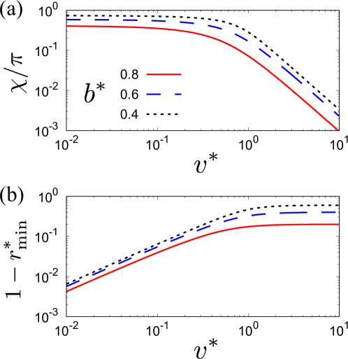
Figure 16: Velocity dependence of (a) the scattering angle $\chi$ and (b) the closest distance $r_{\mathrm{min}}$ against the dimensionless relative speed $v^{*}$ for $b^{*}\equiv b/d=0.4$, $0.6$, and $0.8$. Here, we have introduced $r_{\mathrm{min}}^{*}\equiv r_{\mathrm{min}}/d$.

Appendix C Comparison between Cauchy’s contact stress and the collisional contribution to the stress in a hard-core system

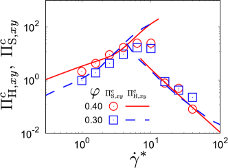
Figure 17: Shear rate dependence of the contact shear stresses $\Pi^{c}_{\mathrm{H},xy}$ and $\Pi^{c}_{\mathrm{S},xy}$ for $\varphi=0.30$ and $0.40$ by fixing $\xi_{\mathrm{env}}=1.0$ and $\varepsilon^{*}=10^{4}$. The lines represent the theoretical results $\Pi_{\mathrm{H},xy}^{c}$ obtained from Eq. (29). The symbols correspond to the simulation results $\Pi_{\mathrm{S},xy}^{c}$ obtained from Eq. (7).

In this appendix, we examine the validity of $\Pi_{\mathrm{H},xy}^{c}$ in Eq. (47) with Eq. (38) used for the theoretical analysis to evaluate the contact stress $\Pi_{\mathrm{S},xy}^{c}$ for the soft-core systems Eq. (9) with (7) from the comparison between two expressions. Figure 17 illustrates that $\Pi_{\mathrm{H},xy}^{c}$ is reasonably close to $\Pi_{\mathrm{S},xy}^{c}$ in the wide range of the parameters’ space. This is the indirect evidence of the validity of the replacement of Eq. (7) by Eq. (29), although we cannot justify this treatment theoretically.

Appendix D Convergence of $\Lambda_{\alpha\beta}^{*}$ and $\Pi_{\mathrm{H},xy}^{c}$ in the expansions of $\tilde{\dot{\gamma}}$ and the linear theory

In this appendix, we show how the calculated stress depends on the number of truncation terms $N_{\mathrm{c}}$ in the set of equations (43). We also present some analytic results of the linear theory with $N_{\mathrm{c}}=1$.

D.1 Convergence of expansions

In this subsection, we present how the expansions of $\Lambda_{\alpha\beta}^{*}$ and $\Pi_{\mathrm{H},xy}^{c}$ in the set of equations (43) converge as the number of $N_{\mathrm{c}}$ increases.

We plot the theoretical viscosity $\eta^{*}$ against $\dot{\gamma}^{*}$ for various $N_{\mathrm{c}}$ in Fig. 18 with $\varphi=0.30$, $\xi_{\mathrm{env}}=1.0$, and $\varepsilon^{*}=10^{4}$. We illustrate that the difference between viscosity obtained by $N_{\mathrm{c}}=2$ and that by $N_{\mathrm{c}}=6$ is invisible, although the linear theory with $N_{\mathrm{c}}=1$ deviates from those for $N_{\mathrm{c}}\geq 2$. We also obtain the similar results for $\theta$. Thus, we adopt $N_{\mathrm{c}}=2$ for the calculations in the main text. We note that it is possible to get analytic expressions of $\eta^{*}$ and $\theta$ in the case of $N_{\mathrm{c}}=1$ as shown in the next subsection, while it is impossible to obtain the analytic expressions if we adopt $N_{\mathrm{c}}\geq 2$.

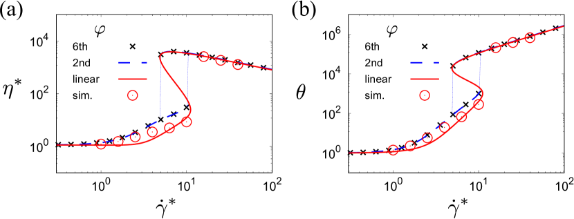
Figure 18: Plots of (a) $\eta^{*}$ and (b) $\theta$ against $\dot{\gamma}^{*}$ for $\varphi=0.30$, $\xi_{\mathrm{env}}=1.0$, and $\varepsilon^{*}=10^{4}$ when we control the truncation $N_{\mathrm{c}}=1$ (solid line), $2$ (dashed line), and $6$ (crosses).

D.2 Linear theory

In this subsection, let us show the explicit forms when we only consider the terms up to the linear order with respect to the expansion parameter $\tilde{\dot{\gamma}}$ (i.e. $N_{\mathrm{c}}=1$) in the set of equations (43). A set of dynamical equations (44) in the steady state with $N_{\mathrm{c}}=1$ is reduced to (see also Ref. [36]):

$$\frac{2\dot{\gamma}^{*}}{3}{\cal C}\Pi_{xy} =2(\theta-1),$$ (85a)

$$2\dot{\gamma}^{*}\Pi_{xy} =(2+\nu^{*})\Delta\theta,$$ (85b)

$$2\dot{\gamma}^{*}{\cal E}\Pi_{xy} =(2+\nu^{*})\delta\theta,$$ (85c)

$$-(2+\nu^{*})\Pi_{xy} =\dot{\gamma}^{*}\left(\frac{2}{3}{\cal D}\Delta\theta-\frac{1}{3}{\cal E}\delta\theta-{\cal C}\theta\right),$$ (85d)

with

$${\cal C} \equiv 1+\frac{8}{5}\varphi g_{0}\Omega_{2,2}^{*},$$ (86a)

$${\cal D} \equiv 1-\frac{4}{35}\varphi g_{0}\Omega_{2,2}^{*},$$ (86b)

$${\cal E} \equiv 1-\frac{16}{35}\varphi g_{0}\Omega_{2,2}^{*},$$ (86c)

$$\nu^{*} \equiv\frac{96}{5\sqrt{\pi}}g_{0}\varphi\xi_{\mathrm{env}}\sqrt{\theta}\Omega_{2,2}^{*}.$$ (86d)

We note that these quantities are equivalent to those for hard-core systems [36, 37, 80, 40, 72] for $\Omega_{2,2}^{*}\to 1$. The set of solutions of Eqs. (85) is given by

$$\Pi_{xy} =\frac{3}{\dot{\gamma}^{*}{\cal C}}(\theta-1),$$ (87a)

$$\Delta\theta =\frac{3}{{\cal C}}\frac{2(\theta-1)}{2+\nu^{*}},$$ (87b)

$$\delta\theta =\frac{3{\cal E}}{{\cal C}}\frac{2(\theta-1)}{2+\nu^{*}}.$$ (87c)

Substituting Eqs. (87) into Eq. (85d), we obtain the expression of $\dot{\gamma}^{*}$ as

$$\dot{\gamma}^{*}=\sqrt{\frac{-3(1-\theta^{-1})(2+\nu^{*})}{{\cal C}{\cal F}}},$$ (88)

where

$${\cal F} \equiv\frac{2}{3}{\cal D}\frac{\Delta\theta}{\theta}-\frac{1}{3}{\cal E}\frac{\delta\theta}{\theta}-{\cal C}=\frac{2{\cal D}-{\cal E}^{2}}{{\cal C}}\frac{2(1-\theta^{-1})}{2+\nu^{*}}-{\cal C}.$$ (89)

Equation (88) is an equation to determine $\dot{\gamma}^{*}$ under a given set of $\varphi$ and $\theta$. Once we fix $\theta$, we can determine the other rheological quantities $\Pi_{xy}$, $\Delta\theta$, and $\delta\theta$ from Eqs. (87a)–(87c), respectively. Correspondingly, the collisional contribution to the shear stress is given by

$$\Pi_{\mathrm{H},xy}^{c}=\frac{8}{5}\varphi g_{0}\Omega_{2,2}^{*}\left(\Pi_{xy}+\frac{1}{\sqrt{\pi}}\frac{\dot{\gamma}^{*}}{\xi_{\mathrm{env}}\sqrt{\theta}}\right).$$ (90)

This quantity is also equivalent to that for hard-core systems for $\Omega_{2,2}^{*}\to 1$ [36, 37].

Appendix E Evaluation of the collision moment in dilute soft-core systems

In this appendix, we present the evaluation $\overleftrightarrow{\Lambda}$ in dilute soft-core systems [38, 71, 81] to clarify the difference between the dilute system and the moderately dense system analyzed in this paper. Note that the results presented in this appendix implicitly used Ref. [38] but it does not contain any explicit expressions.

Because the two-body distribution function does not include the information of positions, the collision integral $J[\bm{V}|f^{(2)}(1,2)]$ is given by

$$J[\bm{V}|f^{(2)}(1,2)] \simeq\int d\bm{V}_{2}\int d\bm{\Omega}\mathcal{S}(\chi,V_{12})V_{12}\left[f^{(2)}(\bm{V}_{1}^{\prime\prime},\bm{V}_{2}^{\prime\prime};t)-f^{(2)}(\bm{V}_{1},\bm{V}_{2};t)\right].$$ (91)

We also assume the decoupling approximation

$$f^{(2)}(\bm{V}_{1},\bm{V}_{2};t)\simeq f(\bm{V}_{1},t)f(\bm{V}_{2},t).$$ (92)

Using this approximation, the collision moment becomes

$$\overleftrightarrow{\Lambda} \equiv 4\times\frac{m}{2}\int d\bm{V}_{1}\int d\bm{V}_{2}\int d\hat{\bm{k}}_{12}\mathcal{S}(\chi,V_{12})(\bm{V}_{12}\cdot\hat{\bm{k}}_{12})^{2}$$

$$\hskip 10.00002pt\times\left[\bm{V}_{12}\hat{\bm{k}}_{12}+\hat{\bm{k}}_{12}\bm{V}_{12}-2(\bm{V}_{12}\cdot\hat{\bm{k}}_{12})\hat{\bm{k}}_{12}\hat{\bm{k}}_{12})\right]f\left(\bm{V}_{1},t\right)f\left(\bm{V}_{2},t\right),$$ (93)

where we have used the tensor representation for later convenience. After introducing the velocity of center-of-gravity and the relative velocity $\bm{V}_{\mathrm{G}}$ and $\bm{V}_{12}=\bm{V}_{1}-\bm{V}_{2}$ with

$$\bm{V}_{\mathrm{G}}\equiv\frac{\bm{V}_{1}+\bm{V}_{2}}{2},$$ (94)

and $\mathcal{S}(\chi,V)\sin\chi=b|\partial b/\partial\chi|$ into Eq. (93), one obtains

$$\overleftrightarrow{\Lambda} \equiv\frac{m}{2}\int d\bm{V}_{\mathrm{G}}\int d\bm{V}_{12}\int_{0}^{d}db\int_{0}^{2\pi}d\phi\,bV_{12}(\bm{V}_{12}\cdot\hat{\bm{k}}_{12})$$

$$\hskip 10.00002pt\times\left[\bm{V}_{12}\hat{\bm{k}}_{12}+\hat{\bm{k}}_{12}\bm{V}_{12}-2(\bm{V}_{12}\cdot\hat{\bm{k}}_{12})\hat{\bm{k}}_{12}\hat{\bm{k}}_{12})\right]f\left(\bm{V}_{1},t\right)f\left(\bm{V}_{2},t\right).$$ (95)

Here, the angle $\phi$ is the same as that appears in Fig. 2. Using the Grad approximation, $\Lambda_{\alpha\beta}$ is rewritten as

$$\overleftrightarrow{\Lambda} =\frac{1}{2}\pi^{-3}mn^{2}v_{\mathrm{T}}^{3}\int d\bm{C}_{\mathrm{G}}\int d\bm{c}_{12}\int_{0}^{d}db\int_{0}^{2\pi}d\phi\,bc_{12}\left(\bm{c}_{12}\cdot\hat{\bm{k}}_{12}\right)\exp\left(-2C_{\mathrm{G}}^{2}-\frac{1}{2}c_{12}^{2}\right)$$

$$\hskip 10.00002pt\times\left[\bm{c}_{12}\hat{\bm{k}}_{12}+\hat{\bm{k}}_{12}\bm{c}_{12}-2\left(\bm{c}_{12}\cdot\hat{\bm{k}}_{12}\right)\hat{\bm{k}}_{12}\hat{\bm{k}}_{12})\right]\left[1-\frac{\Pi_{\alpha\beta}}{\theta}\left(2C_{\mathrm{G},\alpha}C_{\mathrm{G},\beta}+\frac{1}{2}c_{12,\alpha}c_{12,\beta}\right)\right]$$

$$=2(2\pi)^{-3/2}mn^{2}v_{\mathrm{T}}^{3}\int d\bm{c}_{12}\int_{0}^{d}db\int_{0}^{2\pi}d\phi\,bc_{12}\left(\bm{c}_{12}\cdot\hat{\bm{k}}_{12}\right)\exp\left(-\frac{1}{2}c_{12}^{2}\right)$$

$$\hskip 10.00002pt\times\left[\bm{c}_{12}\hat{\bm{k}}_{12}+\hat{\bm{k}}_{12}\bm{c}_{12}-2\left(\bm{c}_{12}\cdot\hat{\bm{k}}_{12}\right)\hat{\bm{k}}_{12}\hat{\bm{k}}_{12}\right]\left(1-\frac{\Pi_{\alpha\beta}}{2\theta}c_{12,\alpha}c_{12,\beta}\right),$$ (96)

where we have introduced the dimensional velocities

$$\bm{C}_{\mathrm{G}}\equiv\frac{\bm{V}_{\mathrm{G}}}{v_{\mathrm{T}}},\quad\bm{c}_{12}\equiv\frac{\bm{V}_{12}}{v_{\mathrm{T}}},$$ (97)

and used $\Pi_{\alpha\alpha}=0$ in the second equality.

Let us introduce the following four quantities:

$$\overleftrightarrow{\Lambda_{1}^{*}} \equiv\int d\bm{c}_{12}\int_{0}^{d}db\int_{0}^{2\pi}d\phi\,bc_{12}\left(\bm{c}_{12}\cdot\hat{\bm{k}}_{12}\right)\exp\left(-\frac{1}{2}c_{12}^{2}\right)\left(\bm{c}_{12}\hat{\bm{k}}_{12}+\hat{\bm{k}}_{12}\bm{c}_{12}\right),$$ (98a)

$$\overleftrightarrow{\Lambda_{2}^{*}} \equiv-2\int d\bm{c}_{12}\int_{0}^{d}db\int_{0}^{2\pi}d\phi\,bc_{12}\left(\bm{c}_{12}\cdot\hat{\bm{k}}_{12}\right)^{2}\exp\left(-\frac{1}{2}c_{12}^{2}\right)\hat{\bm{k}}_{12}\hat{\bm{k}}_{12},$$ (98b)

$$\overleftrightarrow{\Lambda_{3}^{*}} \equiv\frac{\Pi_{\alpha\beta}}{2\theta}\int d\bm{c}_{12}\int_{0}^{d}db\int_{0}^{2\pi}d\phi\,bc_{12}c_{12,\alpha}c_{12,\beta}\left(\bm{c}_{12}\cdot\hat{\bm{k}}_{12}\right)\exp\left(-\frac{1}{2}c_{12}^{2}\right)\left(\bm{c}_{12}\hat{\bm{k}}_{12}+\hat{\bm{k}}_{12}\bm{c}_{12}\right),$$ (98c)

$$\overleftrightarrow{\Lambda_{4}^{*}} \equiv-\frac{\Pi_{\alpha\beta}}{\theta}\int d\bm{c}_{12}\int_{0}^{d}db\int_{0}^{2\pi}d\phi\,bc_{12}c_{12,\alpha}c_{12,\beta}\left(\bm{c}_{12}\cdot\hat{\bm{k}}_{12}\right)^{2}\exp\left(-\frac{1}{2}c_{12}^{2}\right)\hat{\bm{k}}_{12}\hat{\bm{k}}_{12}.$$ (98d)

Using these quantities, we can rewrite Eq. (96) as

$$\overleftrightarrow{\Lambda}=\frac{1}{2}(2\pi)^{-3/2}mn^{2}v_{\mathrm{T}}^{3}\left(\overleftrightarrow{\Lambda_{1}^{*}}+\overleftrightarrow{\Lambda_{2}^{*}}+\overleftrightarrow{\Lambda_{3}^{*}}+\overleftrightarrow{\Lambda_{4}^{*}}\right).$$ (99)

First, we calculate $\overleftrightarrow{\Lambda_{1}^{*}}$. It is convenient to to consider $\bm{c}_{12}$ to be the $z$-axis, and express $\hat{\bm{k}}_{12}$ in the the polar coordinates $(\theta,\phi)$ from $\bm{c}_{12}$. We note that these $\theta$ and $\phi$ are the same as those in Fig. 2. Using these coordinates, it shows the following:

$$\int_{0}^{2\pi}d\phi\left(\bm{c}_{12}\cdot\hat{\bm{k}}_{12}\right)\hat{\bm{k}}_{12} =\int_{0}^{2\pi}d\phi c_{12}\cos\theta\begin{pmatrix}\sin\theta\cos\phi\\ \sin\theta\sin\phi\\ \cos\theta\end{pmatrix}$$

$$=2\pi c_{12}\cos^{2}\theta\begin{pmatrix}0\\ 0\\ 1\end{pmatrix}=2\pi\cos^{2}\theta\bm{c}_{12}.$$ (100)

Then, the quantity $\overleftrightarrow{\Lambda_{1}^{*}}$ becomes

$$\overleftrightarrow{\Lambda_{1}^{*}}\equiv 4\pi\int d\bm{c}_{12}\int_{0}^{d}db\,bc_{12}\cos^{2}\theta\exp\left(-\frac{1}{2}c_{12}^{2}\right)\bm{c}_{12}\bm{c}_{12}.$$ (101)

To calculate further, we express $\bm{c}_{12}$ in the polar coordinates $(c_{12},\theta_{\mathrm{c}},\phi_{\mathrm{c}})$. Equation (101) becomes

$$\overleftrightarrow{\Lambda_{1}^{*}} =4\pi\int_{0}^{\infty}dc_{12}\int_{0}^{d}db\,bc_{12}^{5}\cos^{2}\theta\exp\left(-\frac{1}{2}c_{12}^{2}\right)$$

$$\hskip 10.00002pt\times\int_{0}^{\pi}d\theta_{\mathrm{c}}\int_{0}^{2\pi}d\phi_{\mathrm{c}}\sin\theta_{\mathrm{c}}\begin{pmatrix}\sin^{2}\theta_{\mathrm{c}}\cos^{2}\phi_{\mathrm{c}}&\sin^{2}\theta_{\mathrm{c}}\sin\phi_{\mathrm{c}}\cos\phi_{\mathrm{c}}&\sin\theta_{\mathrm{c}}\cos\theta_{\mathrm{c}}\cos\phi_{\mathrm{c}}\\ \sin^{2}\theta_{\mathrm{c}}\sin\phi_{\mathrm{c}}\cos\phi_{\mathrm{c}}&\sin^{2}\theta_{\mathrm{c}}\sin^{2}\phi_{\mathrm{c}}&\sin\theta_{\mathrm{c}}\cos\theta_{\mathrm{c}}\sin\phi_{\mathrm{c}}\\ \sin\theta_{\mathrm{c}}\cos\theta_{\mathrm{c}}\cos\phi_{\mathrm{c}}&\sin\theta_{\mathrm{c}}\cos\theta_{\mathrm{c}}\sin\phi_{\mathrm{c}}&\cos^{2}\theta_{\mathrm{c}}\end{pmatrix}$$

$$=\frac{16}{3}\pi^{2}\int_{0}^{\infty}dc_{12}\int_{0}^{d}db\,bc_{12}^{5}\cos^{2}\theta\exp\left(-\frac{1}{2}c_{12}^{2}\right)\overleftrightarrow{1},$$ (102)

where $\overleftrightarrow{1}$ is the unit tensor whose size is $3\times 3$.

Similarly, let us consider the following:

$$\int_{0}^{2\pi}d\phi\left(\bm{c}_{12}\cdot\hat{\bm{k}}_{12}\right)^{2}\hat{\bm{k}}_{12}\hat{\bm{k}}_{12} =\int_{0}^{2\pi}d\phi c_{12}^{2}\cos^{2}\theta\begin{pmatrix}\sin^{2}\theta\cos^{2}\phi&\sin^{2}\theta\sin\phi\cos\phi&\sin\theta\cos\theta\cos\phi\\ \sin^{2}\theta\sin\phi\cos\phi&\sin^{2}\theta\sin^{2}\phi&\sin\theta\cos\theta\sin\phi\\ \sin\theta\cos\theta\cos\phi&\sin\theta\cos\theta\sin\phi&\cos^{2}\theta\end{pmatrix}$$

$$=\pi c_{12}^{2}\cos^{2}\theta\begin{pmatrix}\sin^{2}\theta&0&0\\ 0&\sin^{2}\theta&0\\ 0&0&2\cos^{2}\theta\end{pmatrix}$$

$$=\pi\cos^{2}\theta\left[c_{12}^{2}\sin^{2}\theta\overleftrightarrow{1}+\left(2\cos^{2}\theta-\sin^{2}\theta\right)\bm{c}_{12}\bm{c}_{12}\right].$$ (103)

With the aid of this, the quantity $\overleftrightarrow{\Lambda_{2}^{*}}$ is rewritten as

$$\overleftrightarrow{\Lambda_{2}^{*}} =-2\pi\int d\bm{c}_{12}\int_{0}^{d}db\,bc_{12}\cos^{2}\theta\exp\left(-\frac{1}{2}c_{12}^{2}\right)\left[c_{12}^{2}\sin^{2}\theta\overleftrightarrow{1}+\left(2\cos^{2}\theta-\sin^{2}\theta\right)\bm{c}_{12}\bm{c}_{12}\right]$$

$$=-2\pi\int_{0}^{\infty}dc_{12}\int_{0}^{d}db\,bc_{12}^{3}\cos^{2}\theta\exp\left(-\frac{1}{2}c_{12}^{2}\right)\left[4\pi c_{12}^{2}\sin^{2}\theta+\frac{4}{3}\pi\left(2\cos^{2}\theta-\sin^{2}\theta\right)\right]\overleftrightarrow{1}$$

$$=-\frac{16}{3}\pi^{2}\int_{0}^{\infty}dc_{12}\int_{0}^{d}db\,bc_{12}^{5}\cos^{2}\theta\exp\left(-\frac{1}{2}c_{12}^{2}\right)\overleftrightarrow{1}.$$ (104)

Third, the quantity $\overleftrightarrow{\Lambda_{3}^{*}}$ becomes

$$\overleftrightarrow{\Lambda_{3}^{*}}\equiv-\frac{\Pi_{\alpha\beta}}{\theta}2\pi\int d\bm{c}_{12}\int_{0}^{d}db\,bc_{12}\cos^{2}\theta\exp\left(-\frac{1}{2}c_{12}^{2}\right)c_{12,\alpha}c_{12,\beta}\bm{c}_{12}\bm{c}_{12}.$$ (105)

Let us consider the diagonal component $\Lambda_{3,xx}^{*}$.

$$\Lambda_{3,xx}^{*} =\frac{1}{\theta}2\pi\int d\bm{c}_{12}\int_{0}^{d}db\,bc_{12}\cos^{2}\theta\exp\left(-\frac{1}{2}c_{12}^{2}\right)\left(\Pi_{xx}c_{12,x}c_{12,x}+\Pi_{yy}c_{12,y}c_{12,y}+\Pi_{zz}c_{12,z}c_{12,z}\right)c_{12,x}^{2}$$

$$=\frac{\Pi_{xx}}{\theta}\frac{16}{15}\pi^{2}\int_{0}^{\infty}dc_{12}\int_{0}^{d}db\,bc_{12}^{7}\cos^{2}\theta\exp\left(-\frac{1}{2}c_{12}^{2}\right).$$ (106)

Similarly, the nondiagonal component $\Lambda_{3,xy}^{*}$ is obtained as

$$\Lambda_{3,xy}^{*} =\frac{\Pi_{xy}}{\theta}2\pi\int d\bm{c}_{12}\int_{0}^{d}db\,bc_{12}\cos^{2}\theta\exp\left(-\frac{1}{2}c_{12}^{2}\right)2\Pi_{xy}c_{12,x}^{2}c_{12,y}^{2}$$

$$=\frac{\Pi_{xy}}{\theta}\frac{16}{15}\pi^{2}\int_{0}^{\infty}dc_{12}\int_{0}^{d}db\,bc_{12}^{7}\cos^{2}\theta\exp\left(-\frac{1}{2}c_{12}^{2}\right).$$ (107)

We can follow the same procedures for other components. As a result, $\overleftrightarrow{\Lambda_{3}^{*}}$ is evaluated as

$$\overleftrightarrow{\Lambda_{3}^{*}}=\frac{16}{15}\pi^{2}\int_{0}^{\infty}dc_{12}\int_{0}^{d}db\,bc_{12}^{7}\cos^{2}\theta\exp\left(-\frac{1}{2}c_{12}^{2}\right)\frac{\overleftrightarrow{\Pi}}{\theta}.$$ (108)

Fourth, we calculate $\overleftrightarrow{\Lambda_{4}^{*}}$. After some calculation, one reaches

$$\overleftrightarrow{\Lambda_{4}^{*}} =-\frac{16}{15}\pi^{2}\int_{0}^{\infty}dc_{12}\int_{0}^{d}db\,bc_{12}^{7}\cos^{2}\theta\left(1-\frac{3}{2}\sin^{2}\theta\right)\exp\left(-\frac{1}{2}c_{12}^{2}\right)\frac{\overleftrightarrow{\Pi}}{\theta}.$$ (109)

Substituting Eqs. (102), (104), (108), and (109) into Eq. (99), one gets

$$\overleftrightarrow{\Lambda} =-\frac{1}{5}n^{2}T\sqrt{\frac{\pi T}{m}}\int_{0}^{\infty}dc_{12}\int_{0}^{d}db\,bc_{12}^{7}\sin^{2}(2\theta)\exp\left(-\frac{1}{2}c_{12}^{2}\right)\frac{\overleftrightarrow{\Pi}}{\theta}$$

$$=-\nu^{*}\zeta\left(\overleftrightarrow{\sigma^{k}}+p\overleftrightarrow{1}\right),$$ (110)

with the static pressure $p\equiv-\sigma_{\alpha\alpha}^{k}$ and the collision frequency for hard-core system $\nu_{\mathrm{HC}}$ as given in Eq. (86d).

References

- [1] N. J. Wagner and J. F. Brady, Shear thickening in colloidal dispersions, Phys. Today 62, 27 (2009).
- [2] E. Brown and H. M. Jaeger, Shear thickening in concentrated suspensions: phenomenology, mechanisms and relations to jamming, Rep. Prog. Phys. 77, 046602 (2014).
- [3] C. Ness, R. Seto, and R. Mari, The Physics of Dense Suspensions, Ann. Rev. Cond. Mat. Phys. 13, 97 (2022).
- [4] R. Seto, R. Mari, J. F. Morris, and M. M. Denn, Discontinuous Shear Thickening of Frictional Hard-Sphere Suspensions, Phys. Rev. Lett. 111, 218301 (2013).
- [5] H. M. Laun, Normal stresses in extremely shear thickening polymer dispersions, J. Non-Newton. Fluid Mech. 54, 87 (1994).
- [6] C. D. Cwalina and N. J. Wagner, Material properties of the shear-thickened state in concentrated near hard-sphere colloidal dispersions, J. Rheol. 58, 949 (2014).
- [7] M. Otsuki and H. Hayakawa, Critical scaling near jamming transition for frictional granular particles, Phys. Rev. E 83, 051301 (2011).
- [8] D. Bi, J. Zhang, B. Chakraborty, and R. P. Behringer, Jamming by shear, Nature 480, 355 (2011).
- [9] A. Fall, F. Bertrand, D. Hautemayou, C. Mezière, P. Moucheront, A. Lemaítre, and G. Ovarlez, Macroscopic Discontinuous Shear Thickening versus Local Shear Jamming in Cornstarch, Phys. Rev. Lett. 114, 098301 (2015).
- [10] I. R. Peters, S. Majumdar, and H. M. Jaeger, Direct observation of dynamic shear jamming in dense suspensions, Nature 532, 214 (2016).
- [11] M. Otsuki and H. Hayakawa, Shear jamming, discontinuous shear thickening, and fragile states in dry granular materials under oscillatory shear, Phys. Rev. E 101, 032905 (2020).
- [12] Pradipto and H. Hayakawa, Simulation of dense non-Brownian suspensions with the lattice Boltzmann method: shear jammed and fragile states, Soft Matter 16, 945 (2020), [Correction] 18, 685 (2022).
- [13] R. L. Hoffman, Discontinuous and Dilatant Viscosity Behavior in Concentrated Suspensions. I. Observation of a Flow Instability, Trans. Soc. Rheol. 16, 155 (1972).
- [14] R. L. Hoffman, Discontinuous and dilatant viscosity behavior in concentrated suspensions. II. Theory and experimental tests, J. Colloid Interface Sci. 46, 491 (1974).
- [15] R. L. Hoffman, Explanations for the cause of shear thickening in concentrated colloidal suspensions, J. Rheol. 42, 111 (1998).
- [16] M. Wang, S. Jamali, and J. F. Brady, A hydrodynamic model for discontinuous shear-thickening in dense suspensions, J. Rheol. 64, 379 (2020).
- [17] J. F. Brady and G. Bossis, The rheology of concentrated suspensions of spheres in simple shear flow by numerical simulation, J. Fluid Mech. 155, 105 (1985).
- [18] J. F. Brady and G. Bossis, Stokesian Dynamics, Ann. Rev. Fluid Mech. 20, 111 (1988).
- [19] J. Bender and N. J. Wagner, Reversible shear thickening in monodisperse and bidisperse colloidal dispersions, J. Rheol. 40, 899 (1996).
- [20] J. R. Melrose and R. C. Ball, Continuous shear thickening transitions in model concentrated colloids—The role of interparticle forces, J. Rheol. 48, 937 (2004).
- [21] R. S. Farr, J. R. Melrose, and R. C. Ball, Kinetic theory of jamming in hard-sphere startup flows, Phys. Rev. E 55, 7203 (1997).
- [22] T. Kawasaki and L. Berthier, Discontinuous shear thickening in Brownian suspensions, Phys. Rev. E 98, 012609 (2018).
- [23] M. Wyart and M. E. Cates, Discontinuous Shear Thickening without Inertia in Dense Non-Brownian Suspensions, Phys. Rev. Lett. 112, 098302 (2014).
- [24] S. K. Friedlander, Smoke, Dust and Haze: Fundamentals of Aerosol Dynamics, 2nd ed. (Oxford Univ. Press, Oxford, 2000).
- [25] D. L. Koch and R. J. Hill, Inertial Effects in Suspension and Porous-Media Flows, Ann. Rev. Fluid Mech. 33, 619 (2001).
- [26] M. Hu, J. Peng, K. Sun, D. Yue, S. Guo, A. Wiedensohler, and Z. Wu, Estimation of Size-Resolved Ambient Particle Density Based on the Measurement of Aerosol Number, Mass, and Chemical Size Distributions in the Winter in Beijing, Environ. Sci. Technol. 46, 9941 (2012).
- [27] H. Hayakawa and S. Takada, Kinetic theory of discontinuous shear thickening for a dilute gas-solid suspension, Prog. Theor. Exp. Phys. 2019, 083J01 (2019).
- [28] H.-W. Tsao and D. L. Koch, Simple shear flows of dilute gas-solid suspensions, J. Fluid Mech. 296, 211 (1995).
- [29] A. S. Sangani, G. Mo. H.-W. Tsao, and D. L. Koch, Simple shear flows of dense gas-solid suspensions at finite Stokes numbers, J. Fluid Mech. 313, 309 (1996).
- [30] D. L. Koch and A. S. Sangani, Particle pressure and marginal stability limits for a homogeneous monodisperse gas-fluidized bed: kinetic theory and numerical simulations, J. Fluid Mech. 400, 229 (1999).
- [31] D. L. Koch and R. J. Hill, Inertial Effects in Suspension and Porous-Media Flows, Ann. Rev. Fluid Mech. 33, 619 (2001).
- [32] V. Garzó, S. Tennetti, S. Subramaniam, and C. M. Hrenya, Enskog kinetic theory for monodisperse gas-solid flows, J. Fluid Mech. 712, 129 (2012).
- [33] S. Saha and M. Alam, Revisiting ignited-quenched transition and the non-Newtonian rheology of a sheared dilute gas-solid suspension, J. Fluid. Mech. 833, 206 (2017).
- [34] M. Alam, S. Saha, and R. Gupta, Unified theory for a sheared gas-solid suspension: from rapid granular suspension to its small-Stokes-number limit, J. Fluid Mech. 870, 1175 (2019).
- [35] S. Saha and M. Alam, Burnett-order constitutive relations, second moment anisotropy and co-existing states in sheared dense gas-solid suspensions, J. Fluid Mech. 887, 25 (2020).
- [36] H. Hayakawa, S. Takada, and V. Garzó, Kinetic theory of shear thickening for a moderately dense gas-solid suspension: From discontinuous thickening to continuous thickening, Phys. Rev. E 96, 042903 (2017), [Erratum] 101, 069904(E) (2020).
- [37] S. Takada, H. Hayakawa, A. Santos, and V. Garzó, Enskog kinetic theory of rheology for a moderately dense inertial suspension, Phys. Rev. E 102, 022907 (2020).
- [38] S. Sugimoto and S. Takada, Two-Step Discontinuous Shear Thickening of Dilute Inertial Suspensions Having Soft-Core Potential, J. Phys. Soc. Jpn. 89, 084803 (2020), [Addendum] 89, 127001 (2020).
- [39] P. M. Resibois and M. De Leener, Classical Kinetic Theory of Fluids (Wiley, New York, 1977).
- [40] V. Garzó and J. W. Dufty, Dense fluid transport for inelastic hard spheres, Phys. Rev. E 59, 5895 (1999).
- [41] J. F. Lutsko, Transport properties of dense dissipative hard-sphere fluids for arbitrary energy loss models, Phys. Rev. E 72, 021306 (2005).
- [42] V. Garzó, Grad’s moment method for a granular fluid at moderate densities: Navier-Stokes transport coefficients, Phys. Fluids 25, 043301 (2013).
- [43] R. Gómez González and V. Garzó, Influence of the first-order contributions to the partial temperatures on transport properties in polydisperse dense granular mixtures, Phys. Rev. E 100, 032904 (2019).
- [44] V. Garzó, Granular Gaseous Flows —A Kinetic Theory Approach to Granular Gaseous Flows— (Springer, Berlin, 2019).
- [45] S. Takada, K. Hara and H. Hayakawa, Discontinuous Shear Thickening of a Moderately Dense Inertial Suspension of Hydrodynamically Interacting Frictionless Soft Particles, arXiv:2207.05348.
- [46] R. G. González, M. C. Chamorro and V. Garz’o, Rheology of granular particles immersed in a molecular gas under uniform shear flow arXiv:2311.16717.
- [47] B. Derjaguin and L. D. Landau, Theory of the stability of strongly charged lyophobic sols and of the adhesion of strongly charged particles in solutions of electrolytes, Acta Physicochim. URSS 14, 633 (1941).
- [48] E. J. W. Verwey and J. T. G. Overbeek, Theory of the Stability of Lyophobic Colloids: The Interaction of Sol Particles Having an Electric Double Layer (Elsevier, Amsterdam, 1948).
- [49] J. Israelachvili, Intermolecular and Surface Forces, 3rd ed. (Academic Press, New York, 2011).
- [50] T. Kawasaki, A. Ikeda, and L. Berthier, Thinning or thickening? Multiple rheological regimes in dense suspensions of soft particles, EPL 107, 28009 (2014).
- [51] G. Bossis and J. F. Brady, The rheology of Brownian suspensions, J. Chem. Phys. 91, 1866 (1989).
- [52] R. Mari, R. Seto, J. F. Morris, and M. M. Denn, Discontinuous shear thickening in Brownian suspensions by dynamic simulation, Proc. Natl. Acad. Sci. USA 112, 15326 (2015).
- [53] D. J. Evans and G. Morriss, Statistical Mechanics of Nonequilibrium Liquids 2nd ed. (Cambridge Univ. Press, Cambridge, 2008).
- [54] D. J. Evans and G. P. Morriss, Nonlinear-response theory for steady planar Couette flow, Phys. Rev. A 30, 1528 (1984).
- [55] A. W. Lees and S. F. Edwards, The computer study of transport processes under extreme conditions, J. Phys. C: Solid State Phys. 5, 1921 (1972).
- [56] S. Chapman and T. G. Cowling, The Mathematical Theory of Nonuniform Gases 3rd ed. (Cambridge Univ. Press, New York, 1970).
- [57] J. O. Hirschfelder and C. F. Curtiss, Molecular Theory of Gases and Liquids (Wiley, New York, 1954).
- [58] N. F. Carnahan and K. E. Starling, Equation of State for Nonattracting Rigid Spheres, J. Chem. Phys. 51, 635 (1969).
- [59] J. F. Brady and J. F. Morris, Microstructure of strongly sheared suspensions and its impact on rheology and diffusion, J. Fluid Mech. 348, 103 (1997).
- [60] K. Suzuki and H. Hayakawa, Theory for the rheology of dense non-Brownian suspensions: divergence of viscosities and rheology, J. Fluid Mech. 864, 1125 (2019).
- [61] L. Banetta and A. Zaccone, Radial distribution function of Lennard-Jones fluids in shear flows from intermediate asymptotics Phys. Rev. E 99, 052606 (2019).
- [62] H. Grad, On the kinetic theory of rarefied gases, Commun. Pure Appl. Math. 2, 331 (1949).
- [63] M. Torrilhon, Modeling Nonequilibrium Gas Flow Based on Moment Equations, Ann. Rev. Fluid Mech. 48, 429 (2016).
- [64] V. Garzó, Tracer diffusion in granular shear flows, Phys. Rev. E 66, 021308 (2002).
- [65] M. G. Chamorro, F. Vega Reyes, and V. Garzó, Non-Newtonian hydrodynamics for a dilute granular suspension under uniform shear flow, Phys. Rev. E 92, 052205 (2015).
- [66] S. Takada, H. Hayakawa, and A. Santos, Mpemba effect in inertial suspensions, Phys. Rev. E 103, 032901 (2021).
- [67] S. Takada, H. Hayakawa, and V. Garzó, Rheology of a dilute binary mixture of inertial suspension under simple shear flow Prog. Theor. Exp. Phys. 2023, ptad126 (2023).
- [68] C. K. K. Lun, S. B. Savage, D. J. Jeffrey, and N. Chepurnity, Kinetic theories for granular flow: inelastic particles in Couette flow and slightly inelastic particles in a general flowfield, J. Fluid Mech. 140, 223 (1984).
- [69] J. T. Jenkins and M. W. Richman, Kinetic theory for plane flows of a dense gas of identical, rough, inelastic, circular disks, Phys. Fluids 28, 3485 (1985).
- [70] J. T. Jenkins and M. W. Richman, Grad’s 13-moment system for a dense gas of inelastic spheres, Arch. Ration. Mech. Anal. 87, 355 (1985).
- [71] S. Takada and H. Hayakawa, Rheology of dilute cohesive granular gases, Phys. Rev. E 97, 042902 (2018).
- [72] A. Santos, V. Garzó, and J. W. Dufty, Inherent rheology of a granular fluid in uniform shear flow, Phys. Rev. E 69, 061303 (2004).
- [73] S. Takada, Homogeneous cooling and heating states of dilute soft-core gases under nonlinear drag, EPJ Web Conf. 249, 04001 (2021).
- [74] J. M. Montanero, V. Garzó, A. Santos, and J. J. Brey, Kinetic theory of simple granular shear flows of smooth hard spheres, J. Fluid Mech. 389, 391 (1999).
- [75] A. Santos, J. M. Montanero, J. W. Dufty, and J. J. Brey, Kinetic model for the hard-sphere fluid and solid, Phys. Rev. E 57, 1644 (1998).
- [76] S. Iizuka, S. Takada, and H. Hayakawa, in preparation.
- [77] J. A. McLennan, Introduction to Nonequilibrium Statistical Mechanics (Prentice Hall, New Jersey, 1989).
- [78] R. Zwanzig, Nonequilibrium Statistical Mechanics (Oxford Univ. Press, New York, 2001).
- [79] M. Abramowitz and I. A. Stegun, Handbook of Mathematical Functions: With Formulas, Graphs, and Mathematical Tables (Dover, New York, 1964).
- [80] J.-P. Hansen and I. R. McDonald, Theory of Simple Liquids (Academic Press, Cambridge, 2006).
- [81] S. Sugimoto, Bachelor thesis in Department of Mechanical Systems Engineering, Tokyo University of Agriculture and Technology (2020).