Constraining the primordial curvature perturbation using dark matter substructure

Abstract

We investigate the primordial curvature perturbation by the observation of dark matter substructure. Assuming a bump in the spectrum of the curvature perturbation in the wavenumber of $k>1~{}{\rm Mpc}^{-1}$, we track the evolution of the host halo and subhalos in a semianalytic way. Taking into account possible uncertainties in the evaluation of the tidal stripping effect on the subhalo growth, we find a new robust bound on the curvature perturbation with a bump from the number of observed dwarf spheroidal galaxies in our Galaxy and the observations of the stellar stream. The upper limit on the amplitude of the bump is $\order{10^{-7}}$ for $k\sim 10^{3}~{}{\rm Mpc}^{-1}$. Furthermore we find the boost factor, which is crucial for the indirect detection of dark matter signals, is up to $\order{10^{4}}$ due to the bump that is allowed in the current observational bounds.

Introduction: The observation of the cosmic microwave background (CMB) radiation strongly supports inflation at the early stage of the Universe. The CMB observation constrains the amplitude $A_{s}$ and the spectral index $n_{s}$ of the scalar perturbation as $A_{s}=(2.099\pm 0.029)\times 10^{-9}$ and $n_{s}=0.9649\pm 0.0042$ at the pivot scale $k_{*}=0.05~{}{\rm Mpc}^{-1}$ [1]. At a smaller scale, on the other hand, the constraint on the curvature perturbation is relaxed. For instance, the amplitude for the wavenumber of $k>\order{1}~{}{\rm Mpc}^{-1}$ is constrained by $\mu$- and $y$-type distortions in the CMB observation [2, 3], the overproduction of the primordial black holes (PBHs) [4, 5, 6, 7, 8, 9], density profile of ultracompact minihalos [10, 11], the free-free emission in the Planck foreground analysis [12], galaxy luminosity function [13, 14], and gravitational lensing [15]. Despite the constraints, the scalar amplitude in the small scale can be much larger than $\order{10^{-9}}$. In this paper, we point out that the curvature perturbation in such a small scale gives impact on the evolution of the hierarchical structures of galaxies, which is traced by dark matter halos of the Universe.

Dark matter plays a crucial role in the structure formation; the quantum fluctuation produced by inflation seeds the density fluctuation, which grows in the gravitational potential of dark matter. Therefore the imprint of the small-scale perturbation during the inflation is expected to remain in the current structure of dark matter halos. Subhalos, which reside in larger-scale halos, are especially promising objects to reveal the nature of dark matter. Dwarf spheroidal galaxies (dSphs) can form inside subhalos and they have been found and observed intensively these days in the prospects to detect dark matter annihilation signals [16, 17, 18].

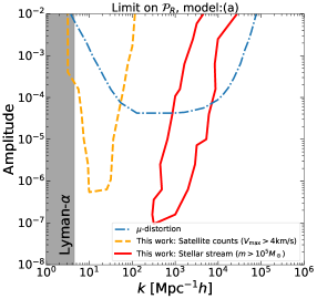
Figure 1: Excluded region on the primordial curvature perturbation. The tidal model (a) is adopted. Upper regions separated by lines are excluded at 95% C.L. “Satellite counts” (orange, dashed) and “Stellar stream ” (red, dashed) correspond to the limits by the observed number of dSphs and the observation of the stellar stream, respectively. See Eqs. (9) and (10). As a reference, the constraint due to $\mu$-distortion is shown as “$\mu$-distortion”, which is given in Ref. [6]. Shaded region on the left is disfavored from the Lyman-$\alpha$ observations [19].

In this paper we study the cosmological consequences of the primordial curvature perturbation in the small scale. Assuming an additional bump in the curvature perturbation, we investigate the subhalo evolution by extending the SASHIMI package, a theoretically motivated model for the tidal stripping process calibrated by the $N$-body simulation [20, 21]. We give a new conservative and robust bound on the curvature perturbation by using the observed number of the dSphs in the Galactic halo [22, 23] and the observations of the stellar stream [24, 25]. Our main result is shown in Fig. 1. Additionally we give the predictions for the annihilation boost factor, which will be useful for future study to search for the nature of dark matter.

Throughout the paper, we adopt the cosmological parameters based on the Planck 2018 results [1] (TT,TE,EE+lowE+lensing); the density parameter of dark matter $\Omega_{\rm dm}h^{2}=0.1200$ and that of baryon $\Omega_{\rm b}h^{2}=0.02237$ with $h=0.6736$.

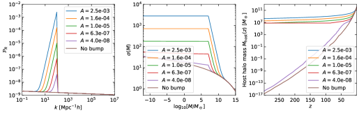
Figure 2: Primordial curvature perturbation ${\cal P}_{R}(k)$ (left), variance $\sigma(M)$ of the power spectrum (middle), and average of host halo mass evolution $M_{\rm host}(z)$ (right). $k_{b}=1.0\times 10^{2}~{}{\rm Mpc}^{-1}h$ is taken for all and each line corresponds to $A=2.5\times 10^{-3}$, $1.6\times 10^{-4}$, $1.0\times 10^{-5}$, $6.3\times 10^{-7}$, and $4.0\times 10^{-8}$. As a reference, the result without the bump is shown as ‘No bump’. $M_{\rm host}(0)=1.3\times 10^{12}M_{\odot}$ is taken for $M_{\rm host}(z)$. See Appendix C for additional figures with different values of $k_{b}$.

The primordial curvature perturbation: We consider a model in which the primordial power spectrum has a bump in the small scale $k\gtrsim\order{1}~{}{\rm Mpc}^{-1}$. In order to investigate the impact of the curvature perturbation in the region, we consider an additional bump on top of the nearly scale-invariant curvature perturbation that is consistent with the CMB observation:

$${\cal P}_{R}={\cal P}_{R}^{(0)}+{\cal P}_{R}^{\rm bump}\,,$$ (1)

where ${\cal P}_{R}^{(0)}(k)=A_{s}(k/k_{*})^{n_{s}-1}$ and

$${\cal P}_{R}^{\rm bump}(k;k_{b})=\left\{\begin{array}[]{ll}(A-{\cal P}_{R}^{(0)}(k_{b}))\left(\frac{k}{k_{b}}\right)^{n_{b}}&k\leq k_{b}\\ 0&k>k_{b}\end{array}\right.\,.$$ (4)

Here we have introduced three parameters, $A$, $k_{b}$, and $n_{b}$. In Ref. [6] the steepest spectral index is $n_{b}=4$ in single-field inflation. On the other hand, Ref. [27] claims that the spectral index can be as large as $8$ after encountering a dip in the amplitude and then the amplitude reaches to a peak with the index less than 4. In our study we adopt $n_{b}=4$ and take $A$ and $k_{b}$ as free parameters. We plot several examples of the ${\cal P}_{R}$ in Fig. 2. The parameters are given in the figure caption.

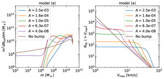
Figure 3: Mass function $dN_{\rm sh}/dm$ of subhalo (left) and cumulative maximum circular velocity function $N_{\rm sh}(>V_{\rm max})$ (right). We take tidal model (a) and the other parameters are the same as Fig. 2. See Appendix C for additional figures with different values of $k_{b}$.

From the curvature perturbation, the variance of the linear power spectrum in the comoving scale $R$ is given by

$$\sigma^{2}(M)=\int d\ln k~{}\frac{k^{3}}{2\pi^{2}}P(k)W^{2}(kR)\,,$$ (5)

where $P(k)$ is the power spectrum calculated from ${\cal P}_{R}$ and $W(kR)$ is the window function. We adopt the sharp-$k$ window, $W(kR)=\Theta(1-kR)$, where $\Theta$ is the Heaviside step function. This is because for the power spectrum that has a steep cutoff, it is shown in Ref. [28] that the sharp-$k$ window gives a good agreement with the simulation. The mass scale $M$ is given as $M=(4\pi/3)(Rc)^{3}\rho_{m}$ where $\rho_{m}=\Omega_{m}\rho_{c}$ ($\rho_{c}$ is the critical density) and a parameter $c=2.7$ is determined by comparing with the simulation [28].

The result of $\sigma(M)$ is given in Fig. 2. It is seen that the bump with $A\gtrsim 10^{-6}$ significantly affects the variance. $\sigma$ is enhanced below a mass scale, which is, for instance, $(4\pi/3)(c/k_{b})^{3}\rho_{m}\sim 10^{7}\,M_{\odot}$ for $k_{b}=10^{2}\,{\rm Mpc}^{-1}h$. The scale gets smaller as $k_{b}$ becomes larger. The variance becomes almost constant for $A\gtrsim 10^{-6}$. This is because the bump contributes dominantly in the integral below the scale $k_{b}$.

The host halo and subhalo evolution: The enhancement on the variance of the power spectrum due to the bump can affect the merger history of both the host and subhalos. To see this we evaluate the halo evolution history based on the extended Press-Schechter (EPS) formalism [30, 31]. See Appendixes A and B for details.

The host halo mass evolution $M_{\rm host}(z)$ is shown in Fig. 2, where the average of 200 host halo realizations is given. We have checked that the result without the bump agrees with the fitting formula given in Ref. [32] in the low $z$ region, which is calibrated against the simulations in $z\lesssim 10$. It is seen that at the low $z$ region the host halo evolution coincides with the one without the bump. However, the difference becomes significant in high $z$ region, especially for a large $A$; we find a plateau for large values of $A$, such as $A\gtrsim 10^{-6}$. In the conventional model, i.e., with no bump in the curvature perturbation, the halos with small mass scales are formed in the past and they grow to massive halos to the present. This is true for the model with bump with a small amplitude, such as $A\lesssim 10^{-8}$. When the amplitude is large, on the other hand, the halo formation and growth happen almost at a certain redshift. For $k_{b}=10^{2}\,{\rm Mpc}^{-1}h$, for instance, halos with mass $\sim 10^{7}\,M_{\odot}$ form at once. We see a mild dependence of the amplitude on the mass scale; the mass scale is larger for the larger amplitude. This is because $\sigma$ is altered in the larger mass-scale region as the amplitude is larger. After the formation they merely grow for some period since $\sigma$ changes drastically for the small-mass scales. This period corresponds to the plateau for $M_{\rm host}$. Eventually, the host mass rebegins to grow in accordance with the case without the bump, which is a reasonable behavior since $\sigma$ coincides with the one calculated without the bump.

The evolution of the subhalos is similar to that of the host halo, but it suffers from the tidal stripping due to the gravitational potential of the host halo after the accretion. To evaluate the subhalo evolution, we modify SASHIMI package to implement the results of $\sigma(M)$ and the host halo evolution $M_{\rm host}(z)$ with the existence of a bump in the primordial curvature perturbation. For consistency, we adopt the concentration-mass relation given by Ref. [33], where the fitting function is given in terms of $\sigma(M)$. In the code the Navarro-Frenk-White (NFW) profile [34] with truncation is assumed, which is characterized by typical mass density $\rho_{\rm s}$, the scale radius $r_{\rm s}$ and the truncation radius $r_{t}$. For the tidal process, we consider three models;

• $g=0.86$ and $\zeta=0.07$ [35],

• $z$-dependent $g(z)$ and $\zeta(z)$ [20],

• no tidal stripping,

where $g$ and $\zeta$ are the parameters in the evolution of the subhalo mass [35]

$$\derivative{m}{t}=-g\frac{m}{\tau_{\rm dyn}}\left(\frac{m}{M(z)}\right)^{\zeta}\,.$$ (6)

Here $\tau_{\rm dyn}$ is the halo’s dynamical time. Since $g(z)$ and $\zeta(z)$ are given in $z\leq 7$ in model (b), we take $g(z)=g(7)$ and $\zeta(z)=\zeta(7)$ for $z>7$ in the current calculation. The model (c) corresponds to the so-called unevolved mass function. We note that the model (c) might be more realistic than the others when we compute the boost factor. This is because the tidal stripping effect may not change the inner structure of the halo profile in the case of a highly concentrated profile [36], which is expected in the current case. The mass distribution function of subhalos at the accretion is given by the EPS formalism as a function of $m_{a}$, $z_{a}$ and the host halo mass $M_{0}$ at $z=z_{0}$. Using the number $d^{2}N_{{\rm sh},a}$ of subhalos with mass $m_{a}$ that accrete at $z=z_{a}$, the subhalo mass function after the tidal stripping is obtained by

$$\frac{dN_{{\rm sh}}}{dm} =\int d^{2}N_{{\rm sh},a}\int dc_{{\rm vir},a}P^{c_{{\rm vir},a}}(m_{a},z_{a})\delta(m-m_{0})\,,$$ (7)

where $P^{c_{{\rm vir},a}}(m_{a},z_{a})$ is the distribution function for $c_{{\rm vir},a}$ that is computed from the one for the concentration-mass relation. A subscript “0” stands for the values at $z=z_{0}$.

We plot the mass function $dN_{\rm sh}/dm$ of the subhalo at $z_{0}=0$ computed using the tidal model (a) in Fig. 3. We found that the mass function is affected significantly, depending on $A$ and $k_{b}$. As $k_{b}$ becomes small, the mass function is altered in the large subhalo mass, which is expected from the behavior of $\sigma(M)$. Due to the bump, the number of the subhalo of a mass scale tends to be enhanced. On the contrary, the mass function is suppressed below that mass scale. This effect is significant for large $A$ and small $k_{b}$. Such a drastic change leads to change the prediction of the number of dSphs, which are formed in subhalos. Additionally, we found that the result is almost independent of the tidal models and $z_{\rm max}$ if $z_{\rm max}\geq 7$. Here $z_{\rm max}$ is the maximum redshift to track the subhalo evolution. Therefore, we expect the observable consequences are determined by the evolution in the low redshift regime and that they are not significantly affected by the details of the tidal evolution models, which we confirm below.

Astrophysical observables and constraint: It is considered that subhalos which satisfy certain conditions form galaxies inside. A quantity for the criterion is the maximum circular velocity. Based on the conventional theory of galaxy formation, for instance, the dSphs formation occurs for $V_{{\rm max},a}>18~{}{\rm km/s}$, where $V_{{\rm max},a}$ is the maximum circular velocity at the time of the accretion. Using this condition, we can predict the number of the present dSphs in the Galaxy, which is one of the important observables of the dSphs. However, this criterion is under debate. A recent study suggests a different criterion of $V_{\rm max,a}>10.5~{}{\rm km/s}$ [37]. Therefore, the predicted number of dSphs can change, depending on the choice of criteria. To avoid such uncertainties on the condition for formation of a dSph, we take a much conservative approach based on the observations. Focusing on the present maximum circular velocity $V_{\rm max}$ that is actually observed for dSphs, the number of dSphs in our Galaxy whose $V_{\rm max}$ is over 4 km/s is given by [38, 39]

$$N_{\rm dSph}^{\rm low}(V_{\rm max}>4~{}{\rm km/s})=94\,.$$ (8)

The condition $V_{\rm max}>4\ {\rm km/s}$ is determined by the minimum of the observed velocity dispersions among dSphs [22, 23]. We apply this observational bound directly to our calculation by imposing the following condition

$$N_{\rm sh}(V_{\rm max}>4~{}{\rm km/s})\geq N_{\rm dSph}^{\rm low}(V_{\rm max}>4~{}{\rm km/s})\,,$$ (9)

and see whether the curvature perturbation with the bump contradicts the observation. Following the method adopted in Ref. [38], we derive 95% C.L. exclusion limit.

Fig. 3 shows the cumulative maximum velocity function $N_{\rm sh}\,(>V_{\rm max})$ of subhalos. It is seen that $N_{\rm sh}\,(>V_{\rm max})$ is enhanced compared to the case with no bump at a large value of $V_{\rm max}$, corresponding to a massive case, as $A$ becomes large and $k_{b}\lesssim 10^{2}\,{\rm Mpc}^{-1}h$. In the exchange for the enhancement at a large $V_{\rm max}$ region, it is suppressed in small $V_{\rm max}$ region. For instance, it is below the observed value for $k_{b}=10^{2}\,{\rm Mpc}^{-1}h$ and $A\gtrsim 2.5\times 10^{-3}$. Therefore, the bump in the primordial curvature perturbation in such a parameter space is excluded. On the other hand, for $k_{b}\gtrsim 10^{2}\,{\rm Mpc}^{-1}h$, the cumulative maximum circular velocity function is almost unchanged. This reflects the fact that the bump with a large $k_{b}$ affects less massive halos than those responsible for dSphs.

Making a comprehensive analysis on the bump model, we compute the cumulative number of the subhalos $N_{\rm sh}\,(V_{\rm max}>4~{}{\rm km/s})$ on the $(A,\,k_{b})$ plane. We found that it is smaller than the observed value in the region $A\gtrsim 10^{-6}$ and $k_{b}\lesssim 10^{2}\,{\rm Mpc}^{-1}h$ so that the region is excluded. The result is shown in Fig. 1. As expected from the results of the mass function, we confirmed that the number of subhalos satisfying the condition of the maximum circular velocity and the resultant exclusion region do not depend on the tidal stripping models. Therefore, it is concluded that the bound is conservative and robust.

Another observable effect appears in the stellar stream, where gaps are caused by a passage of subhalos in the Galaxy. A too large or too small number of subhalos may conflict with the observation of the stellar stream. We make use of the results by Ref. [24], which analyzes the GD-1 stream [25] using data from Gaia [40, 41] and Pan-STARRS survey [42]. We adopt the most conservative limit on the number of subhalos whose mass is within $10^{5}M_{\odot}$ – $10^{9}M_{\odot}$, which is given by

$$N_{\rm sh}/N_{\rm sh,CDM}<2.7~{}(95\%~{}{\rm C.L.})\,,$$ (10)

where $N_{\rm sh,CDM}$ corresponds to the one without the bump. Consequently we found that the amplitude in $k_{b}=\order{10^{2}\,\mathchar 45\relax\,10^{4}}\,{\rm Mpc}^{-1}h$ is constrained; the most stringent upper limit is $10^{-7}$, which is shown in Fig. 1.

The limits from the observations of satellite number and stellar stream for tidal models (b) and (c) are given in Appendix C. We found that the bounds are almost unchanged by choice of the tidal models. Therefore, the limits shown in Fig. 1 are conservative and robust.

Finally we discuss the annihilation boost factor due to the substructure in the host halo. The enhancement of the subhalo clustering leads to a large enhancement of the pair-annihilation signals of dark matter. We define the boost factor as $B\equiv J_{{\rm sh}}^{\rm tot}/J_{\rm h}$, where

$$J_{\rm h}=\int d^{3}x\rho_{\rm h}^{2}\,,~{}~{}J_{\rm sh}^{\rm tot} =\int d\rho_{\rm s}dr_{\rm s}dr_{t}\frac{d^{3}N_{\rm sh}}{d\rho_{\rm s}dr_{\rm s}dr_{t}}\int d^{3}x\rho_{\rm sh}^{2}\,,$$ (11)

assuming the NFW profile $\rho_{\rm h}$ and $\rho_{\rm sh}$ for both the host and subhalos, respectively.

Note that the boost factor depends on the minimum halo mass [33]. In our analysis we take minimum halo mass as $10^{-6}M_{\odot}$, assuming neutralino-like dark matter [43]. We found that the boost factor is significantly enhanced by the amplitude of the bump in the regions which are not excluded from current observations. (See Appendix C for details.) It becomes as large as $\order{10^{4}}$ for $A\sim\order{10^{-2}}$ and $k_{b}\sim\order{10^{5}}$ Mpc${}^{-1}h$. Additionally, we observe a mild dependence on $k_{b}$, i.e, the boost factor gets larger for larger $k_{b}$.

Careful readers may think that the resultant boost factor in the model (c) should be enhanced compared to the model (a) or (b) since the tidal stripping process reduces the subhalo mass. Although the subhalos lose their masses due to the tidal process, the inner structure of the subhalo is hardly affected. This is because the concentration parameter is much larger than $\order{1}$ [33]. The concentration-mass relation at high redshifts is still under debate (e.g., see Ref.  [44]). Hence the model of the concentration-mass relation would be the main source of the uncertainty in the estimation of the boost factor. If the issue is settled, then the clustering of subhalos would be another important observable to constrain the unconventional curvature perturbation in the future experiment.

Conclusion: In this work, we propose a new scheme for investigating the primordial curvature perturbation of the small scale by using the observation of the dark matter substructure. Assuming an additional bump in the primordial curvature perturbation, an enhancement on the variance of the linear power spectrum appears. We track the evolution of both the host halo and subhalos from the power spectrum, based on the EPS formalism and the semianalytic calculation. In the evolution of the subhalo, we take into account uncertainty in the evaluation of the tidal stripping effect by comparing three types of models. We have found that the extra bump in the curvature perturbation significantly affects the evolution of the host and subhalos, depending on the amplitude and the wavenumber scale of the bump. On the other hand, it turns out that the mass functions of the subhalos merely depend on the tidal models. This fact enables us to compute the number of dSphs that is free from the uncertainty in the tidal models. We focus on the cumulative number of subhalos with maximum circular velocity over $4~{}{\rm km/s}$, which is observed directly. Imposing the most conservative bound from observations of the dSphs, we have found that the bump with amplitude $A\gtrsim 10^{-6}$ in $k\lesssim 10^{2}~{}{\rm Mpc}^{-1}h$ is excluded. Another consequence that has a direct connection with the number of subhalos is the stellar stream. Adopting the most conservative limit from the observation, the amplitude of the bump in the region $k=\order{10^{2}\,\mathchar 45\relax\,10^{4}}\,{\rm Mpc}^{-1}h$ is constrained as $A\gtrsim 10^{-7}$ at most. We also obtain an indication for the boost factor, which is crucially important for detecting dark matter annihilation signals. The boost factor of $\order{10^{4}}$ can be expected in the parameter region allowed by the existing observations. In the future, the predictions in this work could be tested by various probes of small-scale halos, such as gravitational lensing observations [45, 46, 47, 48, 49] or pulsar timing array experiments [50, 51, 52, 53, 54, 55]. We leave it for future work.

Appendix A The extended Press-Schechter formalism

The collapse of the overdensity to form the halos is characterized by two quantities:

$$\delta(z)=\delta_{c}/D(z)\,,~{}~{}~{}\sigma(M)\,,$$ (12)

where $z$ is the redshift, $\delta_{c}\simeq 1.686$ is the critical overdensity, and $D(z)$ is the linear growth factor defined by

$$D(z)=D_{\rm norm}H(z)\int_{z}^{\infty}dz^{\prime}\,\frac{1+z^{\prime}}{H^{3}(z^{\prime})}\,.$$ (13)

Here $D_{\rm norm}$ is determined to satisfy $D(0)=1$ and $H(z)$ is the Hubble parameter. Since $D(z)$ is monotonically decreasing function of $z$, $\delta(z)$ monotonically decreases as $z$ gets small. On the other hand, $\sigma(M)$ is cumulative as $M$ becomes small. Namely, the parameters $z$ and $M$ can be translated into $\delta(z)$ and $\sigma(M)$, respectively. Based on the EPS theory, the evolution of the halo is described by the following probability distribution function (PDF) [56, 57, 30],

$$f(S_{2},\delta_{2}|S_{1},\delta_{1})=\frac{1}{\sqrt{2\pi}}\frac{\delta_{2}-\delta_{1}}{\left(S_{2}-S_{1}\right)^{3/2}}\exp\left[-\frac{\left(\delta_{2}-\delta_{1}\right)^{2}}{2\left(S_{2}-S_{1}\right)}\right]\,,$$ (14)

where $S_{i}\equiv\sigma^{2}(M_{i})$ and $\delta_{i}\equiv\delta(z_{i})$ and $z_{1}<z_{2}$. Namely, $f(S_{2},\delta_{2}|S_{1},\delta_{1})$ is the PDF where a halo with a mass of $M_{2}$ is a progenitor at $z=z_{2}$ of a halo with a mass of $M_{1}$ at $z=z_{1}$. In the canonical $\Lambda$CDM case, halos with small mass are created in the past and evolve by accretions and mergers to the present. With the additional bump in the primordial curvature perturbation, however, this picture changes.

In the calculation, we construct the evolution history of the host halo by applying the inverse function method to the above distribution function (see details for Ref. [58]). We start our calculation of the host halo evolution from $z=0$ and track its merger history up to $z=300$, taking 4000 points of a constant interval in the $\ln(1+z)$ space. Considering the Milky Way-like host halo at $z=0$, we take the host halo mass as $M_{\rm host}(z=0)=1.3\times 10^{12}M_{\odot}$ [59].

Appendix B Subhalo evolution

To begin with, we collect important quantities for the subhalo properties. We assume that the halos follow the Navarro-Frenk-White (NFW) profile [34] with truncation, which is characterized by typical mass density $\rho_{\rm s}$, the scale radius $r_{\rm s}$ and the truncation radius $r_{t}$ as

$$\rho_{\rm NFW}(r)=\left\{\matrixquantity{\frac{\rho_{\rm s}}{(r/r_{\rm s})(1+r/r_{\rm s})^{2}}&~{}~{}~{}~{}r\leq r_{t}\\ 0&~{}~{}~{}~{}r>r_{t}}\right.\,.$$ (15)

Given a mass parameter $m_{200}$, a concentration parameter $c_{200}$ is evaluated in the simulations at the redshift $z$. Since $\sigma(M)$ is significantly altered by the bump compared to the conventional case, we adopt the concentration-mass relation given by Ref. [33], where the fitting function is given in terms of $\sigma(M)$. On the other hand, $m_{200}$ relates to $r_{200}$ via $m_{200}=(4\pi/3)200\rho_{c}(z)r_{200}^{3}$, where $\rho_{c}(z)$ is the critical density at the redshift $z$. Using the relation $c_{200}=r_{200}/r_{\rm s}$, the scale radius $r_{\rm s}$ is determined. Then, $\rho_{\rm s}$ is obtained as

$$m =\int d^{3}x\,\rho=4\pi\rho_{\rm s}r_{\rm s}^{3}f(c)\,,$$ (16)

where $f(c)=\ln(1+c)-c/(1+c)$ and $m=m_{200}$ and $c=c_{200}$ are taken. We consider the $(r_{\rm s},\rho_{\rm s})$ as the values at the accretion of a subhalo onto a host halo, which are denoted as $(r_{{\rm s},a},\rho_{{\rm s},a})$. In order to discuss the tidal stripping process of subhalo after the accretion, it is appropriate to use the virial mass $m_{{\rm vir},a}$ instead of $m_{200}$. $m_{{\rm vir},a}$ is obtained by using Eq. (16) where $m=m_{{\rm vir},a}$ and $c=c_{{\rm vir},a}=r_{{\rm vir},a}/r_{{\rm s},a}$, and by

$$m_{{\rm vir},a} =\frac{4\pi}{3}\Delta_{c}(z_{a})\rho_{c}(z_{a})r_{{\rm vir},a}^{3}\,.$$ (17)

Here $\Delta_{c}(z)$ is given in Ref. [63]. To sum up, we get the parameters $\rho_{{\rm s},a}$, $r_{{\rm s},a}$ and $m_{{\rm vir},a}$ at the accretion.

After accretion, the subhalo loses its mass due to the tidal stripping. Given a value of the subhalo mass $m_{0}$ at the redshift $z_{0}$ after tidal stripping, $(\rho_{{\rm s},a},r_{{\rm s},a})$ are translated into $(\rho_{{\rm s},0},r_{{\rm s},0})$ at the redshift $z_{0}$ using the relation among $V_{{\rm max},0}/V_{{\rm max},a}$, $r_{{\rm max},0}/r_{{\rm max},a}$, and $m_{0}/m_{{\rm vir},a}$ [64]. Here $V_{\rm max}$ and $r_{\rm max}$ are the maximum circular velocity and the radius which relate to the NFW profile parameters as

$$V_{\rm max}=\sqrt{\frac{4\pi G\rho_{\rm s}}{4.625}}r_{\rm s}\,,~{}~{}~{}r_{\rm max}=2.163r_{\rm s}\,,$$ (18)

where $G$ is the Newtonian constant. Using Eq. (16) with $m=m_{0}$, $r_{\rm s}=r_{s,0}$, $\rho_{\rm s}=\rho_{{\rm s},0}$, and $c_{t,0}=r_{t,0}/r_{{\rm s},0}$, we obtain the truncation radius $r_{t,0}$ at $z=z_{0}$. To summarize, given a subhalo mass $m_{{\rm vir},a}$ at the accretion and $m_{0}$ after tidal stripping, we obtain subhalo properties, such as $\rho_{\rm s}$, $r_{\rm s}$, $r_{t}$, and $V_{\rm max}$, which are important to discuss the observable consequences.

The mass distribution function ${\cal F}$ of subhalos at the accretion is given by the EPS formalism as a function of $m_{a}$, $z_{a}$ and the host halo mass $M_{0}$ at $z=z_{0}$. Then the number of subhalos with mass $m_{a}$ that accrete at $z=z_{a}$ is given by

$$d^{2}N_{{\rm sh},a}={\cal F}(s_{a},\delta_{a}|S_{0},\delta_{0})d\ln m_{a}dz_{a}\,,$$ (19)

where $s_{a}=\sigma^{2}(m_{a})$, $\delta_{a}=\delta(z_{a})$, $S_{0}=\sigma^{2}(M_{0})$, and $\delta_{0}=\delta(0)$. In the present calculation, $M_{0}=M_{\rm host}(z=0)=1.3\times 10^{12}M_{\odot}$ is taken. Combining all the discussions above, the subhalo mass function after the tidal stripping is obtained by

$$\frac{dN_{{\rm sh}}}{dm}=\int d^{2}N_{{\rm sh},a}\int dc_{{\rm vir},a}P^{c_{{\rm vir},a}}(m_{a},z_{a})\delta(m-m_{0})\,,$$ (20)

where $P^{c_{{\rm vir},a}}(m_{a},z_{a})$ is the distribution function for $c_{{\rm vir},a}$ that is computed from the one for $c_{200}$-mass relation discussed above Eq. (16).

Appendix C Additional figures

We give additional figures with various values of $k_{b}$ for the primordial curvature perturbation ${\cal P}_{R}(k)$ (Fig. 4), the variance $\sigma(M)$ of the power spectrum (Fig. 5), and the average of the host halo mass evolution $M_{\rm host}(z)$ (Fig. 6). The subhalo mass function $dN_{\rm sh}/dm$ and the cumulative maximum circular velocity function $N_{\rm sh}(>V_{\rm max})$ in the tidal model (a), (b), and (c) are shown in Figs. 7 and 8, respectively. Fig. 9 gives the color maps of the cumulative number of subhalos the maximum circular velocity satisfying $V_{\rm max}>4$ km/s, the number of dSphs whose mass is within $10^{5}M_{\odot}$ – $10^{9}M_{\odot}$ normalized by the one without the bump, and the boost factor for the tidal model (a), (b), and (c). The mild dependence of the boost factor on $k_{b}$, which is mentioned in the main text, is seen for all the tidal models. This behavior can be qualitatively understood from the results of the subhalo mass function. In the plot of $dN_{\rm sh}/dm$, the bump is shifted to the smaller scale as $k_{b}$ becomes large; meanwhile, the intensity of $m^{2}dN_{\rm sh}/dm$ stays in the same order. This means that many subhalos with lower masses are formed for bigger $k_{b}$, which leads to the enhancement of the boost factor.

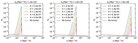
Figure 4: Primordial curvature perturbation ${\cal P}_{R}$ as function of wavenumber. $k_{b}=1.0\times 10^{2}~{}{\rm Mpc}^{-1}h$ (left), $1.0\times 10^{4}~{}{\rm Mpc}^{-1}h$ (center), and $1.0\times 10^{6}~{}{\rm Mpc}^{-1}h$ (right). Each line corresponds to $A=2.5\times 10^{-3}$, $1.6\times 10^{-4}$, $1.0\times 10^{-5}$, $6.3\times 10^{-7}$, and $4.0\times 10^{-8}$ from top to bottom. As a reference, ${\cal P}_{R}^{(0)}$ is shown as ‘No bump’.

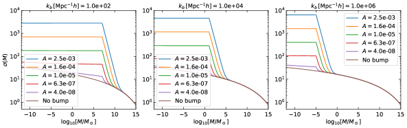
Figure 5: Variance $\sigma$ of the power spectrum as functions of the mass scale $M$. The parameters are the same as Fig. 4. As a reference, $\sigma(M)$ without the bump is shown as ‘No bump’, which is calculated by using CAMB [65].

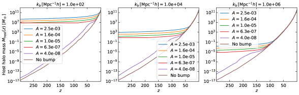
Figure 6: Average of host halo mass evolution as functions of the redshift $z$. We take $M_{\rm host}(z=0)=1.3\times 10^{12}M_{\odot}$ and the other parameters are the same as Fig. 5. The result without the bump is also shown as ‘No bump’.

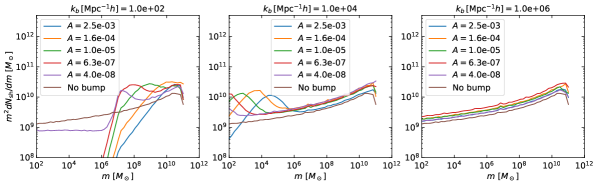
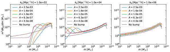
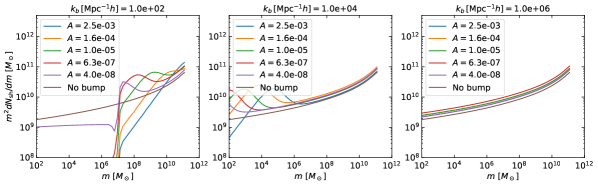
Figure 7: Mass function of subhalo. Tidal model corresponds to (a) Jiang & van den Bosch [35], (b) Hiroshima et al. [20], and (c) no tidal stripping, from top to bottom. The parameters are the same as Fig. 5.

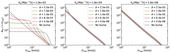
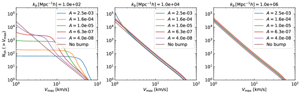
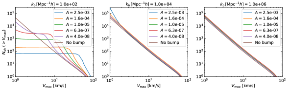
Figure 8: Cumulative maximum circular velocity function. Tidal models, the parameters, and the ordering of panels are the same as Fig. 7.

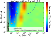
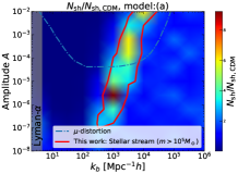
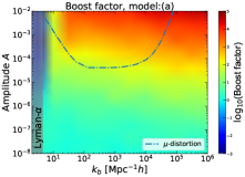
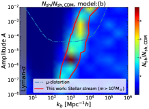
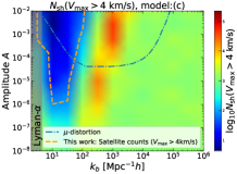
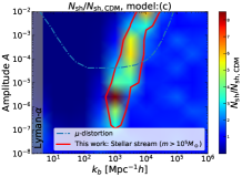
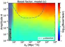
Figure 9: Color map of the cumulative number of subhalos with the maximum circular velocity satisfying $V_{\rm max}>4$ km/s (left) , $N_{\rm sh}/N_{\rm sh,CDM}$ (middle), and boost factor (right) on $(A,\,k_{b})$ plane. For left and right panels, 95% C.L. limits are also shown as in Fig. 1.The tidal models are (a) Jiang & van den Bosch [35], (b) Hiroshima et al. [20], and (c) no tidal stripping, from the top to the bottom. As a reference, the constraint due to $\mu$-distortion is shown as “$\mu$-distortion”, which is given in Ref. [6]. Shaded region on the left is disfavored from the Lyman-$\alpha$ observations [19].

References

- [1] Planck Collaboration, N. Aghanim et al., “Planck 2018 results. VI. Cosmological parameters,” Astron. Astrophys. 641 (2020) A6, arXiv:1807.06209 [astro-ph.CO].
- [2] J. Chluba, A. L. Erickcek, and I. Ben-Dayan, “Probing the inflaton: Small-scale power spectrum constraints from measurements of the CMB energy spectrum,” Astrophys. J. 758 (2012) 76, arXiv:1203.2681 [astro-ph.CO].
- [3] J. Chluba, J. Hamann, and S. P. Patil, “Features and New Physical Scales in Primordial Observables: Theory and Observation,” Int. J. Mod. Phys. D 24 no. 10, (2015) 1530023, arXiv:1505.01834 [astro-ph.CO].
- [4] A. S. Josan, A. M. Green, and K. A. Malik, “Generalised constraints on the curvature perturbation from primordial black holes,” Phys. Rev. D 79 (2009) 103520, arXiv:0903.3184 [astro-ph.CO].
- [5] B. J. Carr, K. Kohri, Y. Sendouda, and J. Yokoyama, “New cosmological constraints on primordial black holes,” Phys. Rev. D 81 (2010) 104019, arXiv:0912.5297 [astro-ph.CO].
- [6] C. T. Byrnes, P. S. Cole, and S. P. Patil, “Steepest growth of the power spectrum and primordial black holes,” JCAP 06 (2019) 028, arXiv:1811.11158 [astro-ph.CO].
- [7] I. Dalianis, “Constraints on the curvature power spectrum from primordial black hole evaporation,” JCAP 08 (2019) 032, arXiv:1812.09807 [astro-ph.CO].
- [8] G. Sato-Polito, E. D. Kovetz, and M. Kamionkowski, “Constraints on the primordial curvature power spectrum from primordial black holes,” Phys. Rev. D 100 no. 6, (2019) 063521, arXiv:1904.10971 [astro-ph.CO].
- [9] A. D. Gow, C. T. Byrnes, P. S. Cole, and S. Young, “The power spectrum on small scales: Robust constraints and comparing PBH methodologies,” JCAP 02 (2021) 002, arXiv:2008.03289 [astro-ph.CO].
- [10] M. S. Delos, A. L. Erickcek, A. P. Bailey, and M. A. Alvarez, “Density profiles of ultracompact minihalos: Implications for constraining the primordial power spectrum,” Phys. Rev. D 98 no. 6, (2018) 063527, arXiv:1806.07389 [astro-ph.CO].
- [11] T. Nakama, T. Suyama, K. Kohri, and N. Hiroshima, “Constraints on small-scale primordial power by annihilation signals from extragalactic dark matter minihalos,” Phys. Rev. D 97 no. 2, (2018) 023539, arXiv:1712.08820 [astro-ph.CO].
- [12] K. T. Abe, T. Minoda, and H. Tashiro, “Constraint on the early-formed dark matter halos using the free-free emission in the Planck foreground analysis,” Phys. Rev. D 105 no. 6, (2022) 063531, arXiv:2108.00621 [astro-ph.CO].
- [13] S. Yoshiura, M. Oguri, K. Takahashi, and T. Takahashi, “Constraints on primordial power spectrum from galaxy luminosity functions,” Phys. Rev. D 102 no. 8, (2020) 083515, arXiv:2007.14695 [astro-ph.CO].
- [14] N. Sabti, J. B. Muñoz, and D. Blas, “Galaxy luminosity function pipeline for cosmology and astrophysics,” Phys. Rev. D 105 no. 4, (2022) 043518, arXiv:2110.13168 [astro-ph.CO].
- [15] D. Gilman, A. Benson, J. Bovy, S. Birrer, T. Treu, and A. Nierenberg, “The primordial matter power spectrum on sub-galactic scales,” Mon. Not. Roy. Astron. Soc. 512 no. 3, (2022) 3163–3188, arXiv:2112.03293 [astro-ph.CO].
- [16] Fermi-LAT, DES Collaboration, A. Albert et al., “Searching for Dark Matter Annihilation in Recently Discovered Milky Way Satellites with Fermi-LAT,” Astrophys. J. 834 no. 2, (2017) 110, arXiv:1611.03184 [astro-ph.HE].
- [17] S. Hoof, A. Geringer-Sameth, and R. Trotta, “A Global Analysis of Dark Matter Signals from 27 Dwarf Spheroidal Galaxies using 11 Years of Fermi-LAT Observations,” JCAP 02 (2020) 012, arXiv:1812.06986 [astro-ph.CO].
- [18] S. Ando, A. Geringer-Sameth, N. Hiroshima, S. Hoof, R. Trotta, and M. G. Walker, “Structure formation models weaken limits on WIMP dark matter from dwarf spheroidal galaxies,” Phys. Rev. D 102 no. 6, (2020) 061302, arXiv:2002.11956 [astro-ph.CO].
- [19] S. Bird, H. V. Peiris, M. Viel, and L. Verde, “Minimally Parametric Power Spectrum Reconstruction from the Lyman-alpha Forest,” Mon. Not. Roy. Astron. Soc. 413 (2011) 1717–1728, arXiv:1010.1519 [astro-ph.CO].
- [20] N. Hiroshima, S. Ando, and T. Ishiyama, “Modeling evolution of dark matter substructure and annihilation boost,” Phys. Rev. D 97 no. 12, (2018) 123002, arXiv:1803.07691 [astro-ph.CO].
- [21] S. Ando, T. Ishiyama, and N. Hiroshima, “Halo Substructure Boosts to the Signatures of Dark Matter Annihilation,” Galaxies 7 no. 3, (2019) 68, arXiv:1903.11427 [astro-ph.CO].
- [22] J. D. Simon, “The Faintest Dwarf Galaxies,” Ann. Rev. Astron. Astrophys. 57 no. 1, (2019) 375–415, arXiv:1901.05465 [astro-ph.GA].
- [23] M. L. M. Collins, E. J. Tollerud, D. J. Sand, A. Bonaca, B. Willman, and J. Strader, “Dynamical evidence for a strong tidal interaction between the Milky Way and its satellite, Leo V,” Mon. Not. Roy. Astron. Soc. 467 no. 1, (2017) 573–585, arXiv:1608.05710 [astro-ph.GA].
- [24] N. Banik, J. Bovy, G. Bertone, D. Erkal, and T. J. L. de Boer, “Evidence of a population of dark subhaloes from and Pan-STARRS observations of the GD-1 stream,” Mon. Not. Roy. Astron. Soc. 502 no. 2, (2021) 2364–2380, arXiv:1911.02662 [astro-ph.GA].
- [25] C. J. Grillmair and O. Dionatos, “Detection of a 63 Degree Cold Stellar Stream in the Sloan Digital Sky Survey,” Astrophys. J. Lett. 643 (2006) L17–L20, arXiv:astro-ph/0604332.
- [26] N. Dalal and C. S. Kochanek, “Strong lensing constraints on small scale linear power,” arXiv:astro-ph/0202290.
- [27] O. Ozsoy and G. Tasinato, “On the slope of the curvature power spectrum in non-attractor inflation,” JCAP 04 (2020) 048, arXiv:1912.01061 [astro-ph.CO].
- [28] A. Schneider, R. E. Smith, and D. Reed, “Halo Mass Function and the Free Streaming Scale,” Mon. Not. Roy. Astron. Soc. 433 (2013) 1573, arXiv:1303.0839 [astro-ph.CO].
- [29] K. Kadota and J. Silk, “Boosting small-scale structure via primordial black holes and implications for sub-GeV dark matter annihilation,” Phys. Rev. D 103 no. 4, (2021) 043530, arXiv:2012.03698 [astro-ph.CO].
- [30] C. G. Lacey and S. Cole, “Merger rates in hierarchical models of galaxy formation,” Mon. Not. Roy. Astron. Soc. 262 (1993) 627–649.
- [31] X. Yang, H. J. Mo, Y. Zhang, and F. C. van den Bosch, “AN ANALYTICAL MODEL FOR THE ACCRETION OF DARK MATTER SUBHALOS,” The Astrophysical Journal 741 no. 1, (Oct, 2011) 13. https://doi.org/10.1088%2F0004-637x%2F741%2F1%2F13.
- [32] C. A. Correa, J. S. B. Wyithe, J. Schaye, and A. R. Duffy, “The accretion history of dark matter haloes – I. The physical origin of the universal function,” Mon. Not. Roy. Astron. Soc. 450 no. 2, (2015) 1514–1520, arXiv:1409.5228 [astro-ph.GA].
- [33] M. A. Sánchez-Conde and F. Prada, “The flattening of the concentration–mass relation towards low halo masses and its implications for the annihilation signal boost,” Mon. Not. Roy. Astron. Soc. 442 no. 3, (2014) 2271–2277, arXiv:1312.1729 [astro-ph.CO].
- [34] J. F. Navarro, C. S. Frenk, and S. D. M. White, “The Structure of cold dark matter halos,” Astrophys. J. 462 (1996) 563–575, arXiv:astro-ph/9508025.
- [35] F. Jiang and F. C. van den Bosch, “Statistics of dark matter substructure – I. Model and universal fitting functions,” Mon. Not. Roy. Astron. Soc. 458 no. 3, (2016) 2848–2869, arXiv:1403.6827 [astro-ph.CO].
- [36] M. S. Delos, “Tidal evolution of dark matter annihilation rates in subhalos,” Phys. Rev. D 100 no. 6, (2019) 063505, arXiv:1906.10690 [astro-ph.CO].
- [37] A. S. Graus, J. S. Bullock, T. Kelley, M. Boylan-Kolchin, S. Garrison-Kimmel, and Y. Qi, “How low does it go? too few galactic satellites with standard reionization quenching,” Monthly Notices of the Royal Astronomical Society 488 no. 4, (Jul, 2019) 4585–4595. https://doi.org/10.1093%2Fmnras%2Fstz1992.
- [38] A. Dekker, S. Ando, C. A. Correa, and K. C. Y. Ng, “Warm Dark Matter Constraints Using Milky-Way Satellite Observations and Subhalo Evolution Modeling,” arXiv:2111.13137 [astro-ph.CO].
- [39] DES Collaboration, A. Drlica-Wagner et al., “Milky Way Satellite Census. I. The Observational Selection Function for Milky Way Satellites in DES Y3 and Pan-STARRS DR1,” Astrophys. J. 893 (2020) 47, arXiv:1912.03302 [astro-ph.GA].
- [40] Gaia Collaboration, A. G. A. Brown et al., “Gaia Data Release 1. Summary of the astrometric, photometric, and survey properties,” Astronomy & Astrophysics 595 (2016) A2.
- [41] Gaia Collaboration, L. Lindegren et al., “Gaia Data Release 2: The astrometric solution,” Astronomy & Astrophysics 616 (2018) A2.
- [42] Pan-STARRA1 Collaboration, K. C. Chambers et al., “The Pan-STARRS1 Surveys,” arXiv:1612.05560 [astro-ph.IM].
- [43] J. Diemand, B. Moore, and J. Stadel, “Earth-mass dark-matter haloes as the first structures in the early Universe,” Nature 433 (2005) 389–391, arXiv:astro-ph/0501589.
- [44] Q. Wang, L. Gao, and C. Meng, “The Ultramarine Simulation: properties of dark matter haloes before redshift 5.5,” arXiv:2206.06313 [astro-ph.CO].
- [45] S. Vegetti, G. Despali, M. R. Lovell, and W. Enzi, “Constraining sterile neutrino cosmologies with strong gravitational lensing observations at redshift z 0.2,” Mon. Not. Roy. Astron. Soc. 481 no. 3, (2018) 3661–3669, arXiv:1801.01505 [astro-ph.CO].
- [46] D. Gilman, S. Birrer, T. Treu, A. Nierenberg, and A. Benson, “Probing dark matter structure down to solar masses: flux ratio statistics in gravitational lenses with line-of-sight haloes,” Mon. Not. Roy. Astron. Soc. 487 no. 4, (2019) 5721–5738, arXiv:1901.11031 [astro-ph.CO].
- [47] D. Gilman, S. Birrer, A. Nierenberg, T. Treu, X. Du, and A. Benson, “Warm dark matter chills out: constraints on the halo mass function and the free-streaming length of dark matter with eight quadruple-image strong gravitational lenses,” Mon. Not. Roy. Astron. Soc. 491 no. 4, (2020) 6077–6101, arXiv:1908.06983 [astro-ph.CO].
- [48] E. O. Nadler, S. Birrer, D. Gilman, R. H. Wechsler, X. Du, A. Benson, A. M. Nierenberg, and T. Treu, “Dark Matter Constraints from a Unified Analysis of Strong Gravitational Lenses and Milky Way Satellite Galaxies,” Astrophys. J. 917 no. 1, (2021) 7, arXiv:2101.07810 [astro-ph.CO].
- [49] N. A. Montel, A. Coogan, C. Correa, K. Karchev, and C. Weniger, “Estimating the warm dark matter mass from strong lensing images with truncated marginal neural ratio estimation,” arXiv:2205.09126 [astro-ph.CO].
- [50] V. S. H. Lee, A. Mitridate, T. Trickle, and K. M. Zurek, “Probing Small-Scale Power Spectra with Pulsar Timing Arrays,” JHEP 06 (2021) 028, arXiv:2012.09857 [astro-ph.CO].
- [51] V. S. H. Lee, S. R. Taylor, T. Trickle, and K. M. Zurek, “Bayesian Forecasts for Dark Matter Substructure Searches with Mock Pulsar Timing Data,” JCAP 08 (2021) 025, arXiv:2104.05717 [astro-ph.CO].
- [52] K. Kashiyama and M. Oguri, “Detectability of Small-Scale Dark Matter Clumps with Pulsar Timing Arrays,” arXiv:1801.07847 [astro-ph.CO].
- [53] M. S. Delos and T. Linden, “Dark Matter Microhalos in the Solar Neighborhood: Pulsar Timing Signatures of Early Matter Domination,” arXiv:2109.03240 [astro-ph.CO].
- [54] H. A. Clark, G. F. Lewis, and P. Scott, “Investigating dark matter substructure with pulsar timing -I. Constraints on ultracompact minihaloes,” Mon. Not. Roy. Astron. Soc. 456 no. 2, (2016) 1394–1401, arXiv:1509.02938 [astro-ph.CO]. [Erratum: Mon.Not.Roy.Astron.Soc. 464, 2468 (2017)].
- [55] T. Ishiyama, J. Makino, and T. Ebisuzaki, “Gamma-ray Signal from Earth-mass Dark Matter Microhalos,” Astrophys. J. Lett. 723 (2010) L195, arXiv:1006.3392 [astro-ph.CO].
- [56] J. R. Bond, S. Cole, G. Efstathiou, and N. Kaiser, “Excursion set mass functions for hierarchical Gaussian fluctuations,” Astrophys. J. 379 (1991) 440.
- [57] R. G. Bower, “The Evolution of groups of galaxies in the Press-Schechter formalism,” Mon. Not. Roy. Astron. Soc. 248 (1991) 332.
- [58] N. Hiroshima, S. Ando, and T. Ishiyama, “Semi-analytical frameworks for subhalos from the smallest to the largest scale,” arXiv:2206.01358 [astro-ph.CO].
- [59] J. Bland-Hawthorn and O. Gerhard, “The Galaxy in Context: Structural, Kinematic, and Integrated Properties,” Ann. Rev. Astron. Astrophys. 54 (2016) 529, arXiv:1602.07702 [astro-ph.GA].
- [60] C. A. Correa, J. S. B. Wyithe, J. Schaye, and A. R. Duffy, “The accretion history of dark matter haloes – III. A physical model for the concentration–mass relation,” Mon. Not. Roy. Astron. Soc. 452 no. 2, (2015) 1217–1232, arXiv:1502.00391 [astro-ph.CO].
- [61] W. Hu and A. V. Kravtsov, “Sample variance considerations for cluster surveys,” Astrophys. J. 584 (2003) 702–715, arXiv:astro-ph/0203169.
- [62] T. Ishiyama, J. Makino, S. Portegies Zwart, D. Groen, K. Nitadori, S. Rieder, C. de Laat, S. McMillan, K. Hiraki, and S. Harfst, “The Cosmogrid Simulation: Statistical Properties of Small Dark Matter Halos,” Astrophys. J. 767 (2013) 146, arXiv:1101.2020 [astro-ph.CO].
- [63] G. L. Bryan and M. L. Norman, “Statistical properties of x-ray clusters: Analytic and numerical comparisons,” Astrophys. J. 495 (1998) 80, arXiv:astro-ph/9710107.
- [64] J. Penarrubia, A. J. Benson, M. G. Walker, G. Gilmore, A. W. McConnachie, and L. Mayer, “The impact of dark matter cusps and cores on the satellite galaxy population around spiral galaxies,” Monthly Notices of the Royal Astronomical Society (May, 2010) no–no. https://doi.org/10.1111%2Fj.1365-2966.2010.16762.x.
- [65] A. Lewis, A. Challinor, and A. Lasenby, “Efficient computation of CMB anisotropies in closed FRW models,” Astrophys. J. 538 (2000) 473–476, arXiv:astro-ph/9911177.