Properties of the Anomalous States of Positronium

Abstract

It is shown that there are anomalous bound-state solutions to the two-body Dirac equation for an electron and a positron interacting via an electromagnetic potential. These anomalous solutions have quantized coordinates at nuclear distances (fermi) and are orthogonal to the usual atomic positronium bound-states as shown by a simple extension of the Bethe-Salpeter equation. It is shown that the anomalous states have many properties which correspond to those of neutrinos.

I Introduction

As shown in previous papers Scott et al. (1992) , Patterson (2019), both the atomic states $\Psi_{Atom}$ and anomalous states $\Psi_{An}$ of positronium admit bound-state solutions to the two-body Dirac equation (TBDE),

$$H\Psi=(H_{0}+\Phi(\rho)\Psi=E\Psi,$$ (1)

with an instantaneous Coulomb potential $\Phi(\rho)=$ $\Phi_{C}=-e^{2}/\rho$, where $H_{0}$ is the free-particle Hamiltonian in the rest frame. By definition, the anomalous states $\Psi_{An}$ are solutions to (1) with $\Phi(\rho)=0$ such that

$$H_{0}\Psi_{An}=0\mathbf{.}$$ (2)

Let the anomalous bound-states $\Psi_{DV}$ be linear combinations of $\Psi_{An}$ which are solutions to (1). From (1) and (2), the $\Psi_{DV}$ are then bound-state solutions to the simple equation

$$\Phi_{C}(\rho)\Psi_{DV}=E\Psi_{DV}.$$ (3)

It was shown in Patterson (2019) that the bound-state solutions to (3) $\Psi_{DV}$ can be found by using the discrete variable (DV) representation Light and Carrington (2000). That is, the solutions to (3) are the DV states $\Psi_{DV}$ in which the coordinate $\rho$ is quantized at discrete separations or $\Psi_{DV}=G\delta(\rho-\rho_{i})$ with $\rho_{i}$ at $fermi$ distances, where the factor $G$ includes the dependence on the other coordinates as well as the spinors. Such DV states can be found by diagonalizing $\Phi_{C}$ in the $\Psi_{An}$ bases only if the $\Psi_{An}$ bases is a complete set in the $\rho$ coordinate. The use of the word ‘discrete’ in DV theory refers to the quantization of the radial coordinate $\rho=\rho_{i}$, in contrast to the normal quantization of momentum for free-particles. Note that the free-particle anomalous states $\Psi_{An}$ in (2) are distinguished from the bound-states $\Psi_{DV}$ of (3) which are comprised of these free-particle states. This distinction has been made because not all anomalous states $\Psi_{An}$ can form a complete set in $\rho$ and can thereby admit bound-states solutions $\Psi_{DV}$ of (1) or (3) using DV theory.

The anomalous bound-states $\Psi_{DV}$, with total angular momentum $J=0$, were shown in Patterson (2019) to have properties which were quite distinct from their atomic counterparts. Besides being bound at nuclear distances $\rho_{i}$, it was found that these DV states are dark and stable. That is, they cannot absorb or emit light, nor can the electron and positron annihilate or dissociate. This unusual behavior was explained by solving both the TBDE and the Bethe-Salpeter equation (BSE) Salpeter and Bethe (1951), Salpeter (1952) with a Coulomb potential. It was found that these DV states $\Psi_{DV}$ form doublets with spin $S_{z}=0$ and energy $E_{i}=-e^{2}/\rho_{i}$

However, in Patterson (2019), it was also found that the Coulomb potential in the TBDE (1) erroneously mixes the anomalous bound-states with the atomic bound-states, resulting in the unusual behavior of the atomic ground-state wavefunction near the origin as found in Scott et al. (1992). This erroneous mixing, while small, was shown not to occur at all for the relativistically correct BSE because of the different time propagation for anomalous bound-states and atomic bound-states. In particular, it was shown, using the BSE, that the time dependence of the atomic states was determined by the two-body Feynman propagator $K_{F}^{2}$, whereas the time dependence of the anomalous states was determined by the two-body retarded propagator $K_{R}^{2}$. As a result, the anomalous bound-states for the instantaneous Coulomb potential were temporally orthogonal to the atomic bound-states and could not be mixed.

It was further argued in Patterson (2019) that the anomalous bound-states were, themselves, both mathematically viable and necessary for completeness in space-time when using the BSE. It seems appropriate that their properties should be investigated further to see if they could exist physically. In Patterson (2019), only the DV states with total angular momentum $J=0$ were considered in order to show their influence on the atomic $J=0$ wavefunctions and energies when using the TBDE. In this paper, the DV states for all $J$ are considered with the restriction to $J_{z}=0$. It is found that there are then four different possible DV states corresponding to a $S=0$ doublet and a $S=1$ doublet for each $J>0$. Like the $J=0$ DV states, these DV states for $J\neq 0$ are also dark and stable. Including the magnetic potential $\Phi_{M}$, the $S=0$ DV doublet has energy $E_{i}^{0}=2e^{2}/\rho_{i}$ and the $S=1$ DV doublet has energy $E_{i}^{1}=0$.

It is also shown that the Lorentz boost reduces the symmetry from spherical $(\rho,\theta)$ to cylindrical $(r,z)$ where $\widehat{z}$ is in the direction of motion. Because of this dynamical symmetry breaking, in the moving frame the DV doublet states with $S_{z}=\pm 1$ can only occur in the $z=0$ plane with $\theta=\pi/2$, so that they are oriented perpendicular to the direction of motion. On the other hand the DV doublet states with $S_{z}=0$ can occur for any $\theta$. Remarkably, using a Lorentz boost for the DV states, it is proven that doublets with $\theta=\pi/2$ transform like Majorana fermions instead of bosons. It is then shown that the $S_{z}=\pm 1$ fermions with mass $M_{i}^{1}=0$ have well defined chirality and helicity as expected for a zero mass fermions.

Finally, it is shown that all of the unusual properties of the anomalous bound-states $\Psi_{DV}$ are a result of the fact that either the electron or the positron (but not both) must be in a negative energy state. As a result, one’s normal understanding of quantum and classical mechanics can be misleading. However, it is shown that these anomalous bound-states still have a simple classical correspondence which aids in understanding their novel properties.

In order to make this paper reasonably self-contained, the notation and the salient developments of the previous work are briefly reviewed below so that the reader can better understand the three equations above. In this review, comparisons are made between the TBDE and the BSE which are especially important to the understanding of the anomalous states.

(Note that the natural units $c=1$ and $\hbar=1$ are used below except for cases where clarity is needed.)

II Review

The Hamiltonian of the TBDE for a free electron and positron, $H_{0}$, in (1) in the moving frame is the sum of the individual Dirac Hamiltonians,

$$H_{0}\Psi=\{\boldsymbol{\alpha}_{e}\cdot\boldsymbol{p}_{e}+\boldsymbol{\alpha}_{p}\cdot\boldsymbol{p}_{p}\text{{\ }}+\text{{\ }}(\gamma_{e4}+\gamma_{p4})m\}\Psi=E\Psi.$$ (4)

Transforming this equation using relative coordinates and their conjugate momenta,

$$\boldsymbol{\rho} =(\mathbf{r}_{e}-\mathbf{r}_{p}),\ \ \boldsymbol{\pi}=\mathbf{(p}_{e}-\mathbf{p}_{p})/2,\$$ (5)

$$\mathbf{R} =(\mathbf{r}_{e}+\mathbf{r}_{p})/2,\ \ \ \mathbf{P}^{\prime}=\mathbf{p}_{e}+\mathbf{p}_{p},$$

one finds Scott et al. (1992), Malenfant (1988),

$$H_{0}\Psi =\{K+\mathcal{M}+\frac{(\boldsymbol{\alpha}_{e}+\boldsymbol{\alpha}_{p})}{2}\cdot\mathbf{P^{\prime}}\}\Psi=E\Psi,$$ (6)

$$K =(\boldsymbol{\alpha}_{e}-\boldsymbol{\alpha}_{p})\cdot\boldsymbol{\pi}\mathbf{,}$$

$$\mathcal{M} =m(\gamma_{e4}+\gamma_{p4}),$$

where $K$ is the two-body kinetic operator and $\mathcal{M}$ is the two-body mass operator. The prime is used for $\mathbf{P^{\prime}}$ to indicate the frame is moving rather than at rest. The matrix elements of $\alpha_{k}$ and $\gamma_{4}$ in the bases of the two Dirac-spinors $\mathbf{e}_{1}$ and $\mathbf{e}_{2}$ are given by

$$\alpha_{k} =i\gamma_{4}\gamma_{k}~{}=\sigma_{k}\left(\begin{array}[c]{cc}0&1\\ 1&0\end{array}\right),\ (for\ k=1,2,3),$$ (9)

$$\gamma_{4} =\left(\begin{array}[c]{cc}1&0\\ 0&-1\end{array}\right),$$ (12)

so that $\alpha_{k}\mathbf{e}_{1}=\sigma_{k}\mathbf{e}_{2},$ $\alpha_{k}\mathbf{e}_{2}=\sigma_{k}\mathbf{e}_{1},$ $\gamma_{4}\mathbf{e}_{1}=\mathbf{e}_{1},$ and $\gamma_{4}\mathbf{e}_{2}=-\mathbf{e}_{2}$. One can then define the four Dirac-spinors $\mathbf{e}_{ij}=\mathbf{e}_{i}\times\mathbf{e}_{j}$ for the direct product wavefunctions $\Psi=\psi(e)\times\psi(p)$ such that

$$\Psi \equiv\binom{{}_{\psi_{1}(e)\psi_{2}(p)}^{\psi_{1}(e)\psi_{1}(p)}}{{}_{\psi_{2}(e)\psi_{2}(p)}^{\psi_{2}(e)\psi_{1}(p)}}\equiv\binom{{}_{\Psi_{12}}^{\Psi_{11}}}{{}_{\Psi_{22}}^{\Psi_{21}}},$$ (13)

$$\equiv\Psi_{11}\mathbf{e}_{11}+\Psi_{12}\mathbf{e}_{12}+\Psi_{21}\mathbf{e}_{21}+\Psi_{22}\mathbf{e}_{22}.$$

With this notation, one finds the simple equations for the mass operators $\gamma_{e4}$ and $\gamma_{p4}$ of $\mathcal{M}$,

$$\gamma_{e4}\Psi =(\Psi_{11}\mathbf{e}_{11}+\Psi_{12}\mathbf{e}_{12}-\Psi_{21}\mathbf{e}_{21}-\Psi_{22}\mathbf{e}_{22}),$$

$$\gamma_{p4}\Psi =(\Psi_{11}\mathbf{e}_{11}-\Psi_{12}\mathbf{e}_{12}+\Psi_{21}\mathbf{e}_{21}-\Psi_{22}\mathbf{e}_{22}).$$

It is useful to use a bases where $\Psi_{g}$ is symmetric and $\Psi_{u}$ is antisymmetric under the simultaneous exchange $\mathbf{e}_{11}\leftrightarrow\mathbf{e}_{22}$ and $\mathbf{e}_{12}\leftrightarrow\mathbf{e}_{21}$, such that

$$\Psi =\Psi_{g}+\Psi_{u},$$ (14)

$$\Psi_{g} =\frac{1}{2}\{(\Psi_{11}+\Psi_{22})(\mathbf{e}_{11}+\mathbf{e}_{22})+(\Psi_{12}+\Psi_{21})(\mathbf{e}_{12}+\mathbf{e}_{21})\},$$

$$\Psi_{u} =\frac{1}{2}\{(\Psi_{11}-\Psi_{22})(\mathbf{e}_{11}-\mathbf{e}_{22})+(\Psi_{12}-\Psi_{21})(\mathbf{e}_{12}-\mathbf{e}_{21})\}.$$

The $\Psi_{g}$ and $\Psi_{u}$ states are only coupled by the mass operator $\mathcal{M}$ in (6) where

$$\mathcal{M}(\mathbf{e}_{11}\pm\mathbf{e}_{22})=2m(\mathbf{e}_{11}\mp\mathbf{e}_{22}).$$ (15)

One can also define the four Pauli-spinors $\chi_{\pm\frac{1}{2}}(e)\chi_{\pm\frac{1}{2}}(p)$ in terms of the states $\Omega_{S_{z}}^{S}$ with total spin $S$ and its $z$ component $S_{z}$, so that

$$\Omega_{0}^{0} =\sqrt{\frac{1}{2}}[\chi_{\frac{1}{2}}(e)\chi_{-\frac{1}{2}}(p)-\chi_{-\frac{1}{2}}(e)\chi_{\frac{1}{2}}(p)],$$ (16)

$$\Omega_{-1}^{1} =\chi_{-\frac{1}{2}}(e)\chi_{-\frac{1}{2}}(p),$$

$$\Omega_{0}^{1} =\sqrt{\frac{1}{2}}[\chi_{\frac{1}{2}}(e)\chi_{-\frac{1}{2}}(p)+\chi_{-\frac{1}{2}}(e)\chi_{\frac{1}{2}}(p)],$$

$$\Omega_{1}^{1} =\chi_{\frac{1}{2}}(e)\chi_{\frac{1}{2}}(p).$$

The singlet state $\Omega_{0}^{0}$ is antisymmetric $(X=-1)$ and triplet states $(\Omega_{-1}^{1},\Omega_{-0}^{1},\Omega_{1}^{1})$ are symmetric $(X=1)$ under particle exchange $\mathbf{X}$, where $\mathbf{X}\Omega_{S_{z}}^{S}=X\Omega_{S_{z}}^{S}$. The Dirac wavefunctions $\Psi$ include terms of the sixteen possible spinors $e_{ij}\Omega_{S_{z}}^{S}$ for the four Dirac-spinors $e_{ij}$ and the four Pauli-spinors $\Omega_{S_{z}}^{S}$.

The free-particle solutions of (6) are direct products $\Psi_{\pm\pm}=\psi_{\pm}(e)\times\psi_{\pm}(p)$ of the single-particle solutions for positive and negative energy states $\psi_{+}$ and $\psi_{-}$ with energies,

$$E_{\pm\pm}=e_{e}+e_{p}=\pm\sqrt{p_{e}^{2}+m^{2}}\pm\sqrt{p_{p}^{2}+m^{2}}.$$

Now let $P^{\prime}$$\mathbf{=}\mathbf{0}$ in (6) so that $H_{0}=K+\mathcal{M}$. Using (5), one finds that $\mathbf{p}_{e}=-\mathbf{p}_{p}$ and $p_{e}^{2}=p_{p}^{2}=\pi^{2}$ where $\mathbf{\pi}$ is the relative momentum. The energies of the free-particle states are then

$$E_{\pm\pm} =\pm e\pm e,$$ (17)

$$e =\sqrt{\pi^{2}+m^{2}}.$$

When using the BSE for $P^{\prime}$$\mathbf{=}\mathbf{0}$, it is useful to divide the free -particle solutions into either atomic states or anomalous states. The atomic free-particle states $\Psi_{Atom}$ have wavefunctions $\Psi_{++}$ and $\Psi_{--}$ Salpeter and Bethe (1951), Salpeter (1952) with energies

$$E_{++}=2e,~{}\ E_{--}=-2e.$$ (18)

The anomalous free -particle states $\Psi_{An}$ have wavefunctions $\Psi_{+-}$ and $\Psi_{-+}$ Patterson (2019) with energies as in (2)

$$E_{+-}=0,~{}\ E_{-+}=0.$$ (19)

Both the atomic bound-states and anomalous bound-states are solutions to the TBDE (1) for $\Phi=\Phi_{C}$. In the momentum representation with a Coulomb potential, one can write (1) (often called the Breit equation) as the integral equation,

$$H_{0}\Psi(\boldsymbol{\pi})-\frac{e^{2}}{2\pi^{2}}\int d^{3}k\frac{1}{\boldsymbol{k\cdot k}}\Psi(\boldsymbol{k+\pi})=E\Psi(\boldsymbol{\pi}).$$ (20)

Note that this equation allows the $\Psi_{Atom}$ and $\Psi_{An}$ states to be mixed by the Coulomb potential. As shown in Patterson (2019), the two different bound-state solutions to (1) or (20), $\Psi_{Atom}$ and $\Psi_{DV}$, have different time behaviors. Together, these two solutions form a complete orthonormal set in space-time. The $\Psi_{Atom}$ and $\Psi_{DV}$ correspond to solutions to two different BSEs which are now described. These two BSEs demonstrate that the Coulomb potential cannot mix the $\Psi_{Atom}$ and $\Psi_{An}$ states.

These two different BSEs are derived from the two-body Green’s functions for the electron and positron propagators in the relative coordinates. Unlike the TBDE, the BSE is relativistically covariant and treats the relative time $t=t_{e}-t_{p}$ and the relative energy $\varepsilon=(e_{e}-e_{p})/2$ of the two particles correctly as the fourth component of the coordinates $\rho=(\boldsymbol{\rho},it)$ and conjugate momenta $\pi=(\boldsymbol{\pi},i\varepsilon)$, respectively. One can define two propagators $K_{F}^{2}=K_{F}(e)\times K_{F}(p)$ and $K_{R}^{2}=K_{R}(e)\times K_{R}(p)$ for the two-body Green’s functions. For the Feynman propagator $K_{F}$, the positive energy states are propagated forward in time, but the negative energy states are propagated backward in time. For the retarded propagator $K_{R}$, both positive and negative energy states are propagated forward in time. For the two equations below, one needs to separate the atomic free -particle states from the anomalous free -particle states as in (18) and (19). For this purpose, the projection operators $\boldsymbol{\Lambda}_{\pm\pm}$ are defined by $\boldsymbol{\Lambda}_{\pm\pm}(\boldsymbol{\pi})\Psi(\boldsymbol{\pi})=\Psi_{\pm\pm}(\boldsymbol{\pi})$.

For atomic bound-states $\Psi_{Atom}$, it is necessary to use the two-body Feynman propagator $K_{F}^{2}$ Salpeter (1952) with the result that the atomic states are only comprised of the free -particle wavefunctions $\Psi_{{}_{++}}(\boldsymbol{\pi})$ and $\Psi_{--}(\boldsymbol{\pi})$ in (18). In the momentum representation, with a Coulomb potential $\Phi_{C}$ , the BSE for $\Psi_{Atom}$ becomes, after some approximations Patterson (2019),

$$H_{0}[\Psi_{{}_{++}}(\boldsymbol{\pi})+\Psi_{--}(\boldsymbol{\pi})]-\frac{e^{2}}{2\pi^{2}}\boldsymbol{\Lambda}_{Atom}\int d^{3}k\frac{1}{\boldsymbol{k\cdot k}}\Psi(\boldsymbol{k+\pi})=E[\Psi_{{}_{++}}(\boldsymbol{\pi})+\Psi_{--}(\boldsymbol{\pi})],$$ (21)

with $\boldsymbol{\Lambda}_{Atom}=\boldsymbol{\Lambda}_{++}(\boldsymbol{\pi})-\boldsymbol{\Lambda}_{--}(\boldsymbol{\pi})$ and $\Psi_{+-}(\boldsymbol{\pi})=\Psi_{-+}(\boldsymbol{\pi})=0$.

For the anomalous bound-states $\Psi_{DV}$, it is necessary to use the two-body retarded propagator $K_{R}^{2}$ Patterson (2019) with the result that the $\Psi_{DV}$ states are only comprised of the anomalous states $\Psi_{{}_{+-}}(\boldsymbol{\pi})$ and $\Psi_{-+}(\boldsymbol{\pi})$ where $H_{0}\Psi_{+-}(\boldsymbol{\pi})=H_{0}\Psi_{-+}(\boldsymbol{\pi})=0$ in (19). Consequently, for a Coulomb potential, one finds the BSE for $\Psi_{DV}$ Patterson (2019) in (1) and (3) is

$$-\frac{e^{2}}{2\pi^{2}}\boldsymbol{\Lambda}_{DV}\int d^{3}k\frac{1}{\boldsymbol{k\cdot k}}\Psi(\boldsymbol{k+\pi})=E[\Psi_{+-}(\boldsymbol{\pi})+\Psi_{-+}(\boldsymbol{\pi})],$$ (22)

with $\boldsymbol{\Lambda}_{DV}=\boldsymbol{\Lambda}_{+-}(\boldsymbol{\pi})+\boldsymbol{\Lambda}_{-+}(\boldsymbol{\pi})$ and $\Psi_{{}_{++}}(\boldsymbol{\pi})=\Psi_{--}(\boldsymbol{\pi})=0$. Note that the BSE (22) for $\Psi_{DV}$ is simply the equivalent of diagonalizing $\Phi_{C}$ in the free-particle bases $\Psi_{+-}(\boldsymbol{\pi})$ and $\Psi_{-+}(\boldsymbol{\pi})$ of $\Psi_{An}$ corresponding to (3). This equation is not correct when the masses of the two particles are unequal as in the case of Hydrogen where $H_{0}\Psi_{+-}(\boldsymbol{\pi})=-H_{0}\Psi_{-+}(\boldsymbol{\pi})\neq 0$. Thus, it only applies to particles with equal masses which obey (2).

One should compare the BSEs (21) and (22) with the TBDE or Breit equation in (20). A consequence of the two BSEs (21) and (22) is that the atomic states $\Psi_{Atom}$ and DV states $\Psi_{DV}$ cannot be mixed by the Coulomb potential in contrast to the TBDE equation (20). Summarizing, one must first eliminate the anomalous free-particle states $\Psi_{+-}$ and $\Psi_{-+}$ in the TBDE (20) in order to calculate the atomic positronium bound-states. Conversely, one must first eliminate the atomic free-particle states $\Psi_{++}$ and $\Psi_{--}$ in the TBDE (20) in order to calculate the positronium DV states.

Mathematically, it must be emphasized that the BSE for $\Psi_{Atom}$ (21) automatically specifies the $K_{F}$ propagator for the atomic bound-states and the BSE for $\Psi_{DV}$ (22) automatically specifies the $K_{R}$ propagator for the anomalous bound-states. One has no choice for the temporal boundary conditions as they are determined by these equations unambiguously. The two different bases formed from atomic and DV states are each mathematically complete sets spatially and therefore overlap: they are not orthogonal spatially. However, they are orthogonal temporally because of their different time behaviors as determined by their different propagators. That is why atomic and DV states cannot be mixed by the instantaneous Coulomb potential.

Physically, the temporal boundary condition arising from the $K_{R}$ propagator is incorrect for free-particle states. As shown by Feynman Feynman (1949), the propagator $K_{F}$ must be used for free electrons and positrons in order to be consistent with the known behavior of these particles undergoing scattering or annihilation. Otherwise, a state $\psi_{+}$ can be scattered into a state $\psi_{-}$ and be lost. Furthermore, QED requires that a state $\psi_{-}$ going backward in time becomes the antiparticle state $\psi_{+}$ going forward in time. For this reason, anomalous states $\Psi_{An}$, which are propagated by $K_{R}$, can only exist as bound-states $\Psi_{DV}$ and not as free-particles. The anomalous bound-states $\Psi_{DV}$ cannot dissociate into free-particles due to the temporal boundary condition imposed by $K_{R}$ on the solutions to (22).

III Discrete Variable (DV) Representation

In this section, it is shown explicitly that there are four different anomalous bound-state solutions $\Psi_{DV}$ to (3) or the equivalent (22), for any $J>0$ corresponding to four orthogonal spinor combinations of $\mathbf{e}_{ij}\Omega_{S_{z}}^{S}.$ In this paper only $J_{z}=0$ states are considered. These four bound-states have radially quantized wavefunctions $\Psi_{DV}=G\delta(\rho-\rho_{i})$ for an instantaneous Coulomb potential $\Phi(\rho)=\Phi_{C}(\rho)$ with energies $E=\Phi(\rho_{i})=-e^{2}/\rho_{i}$. These quantized wavefunctions $\Psi_{DV}$ correspond to the DV representation as reviewed in Light and Carrington (2000). According to DV theory, DV states can be found either numerically, by diagonalizing the potential $\Phi_{C}$ in a complete basis set, or analytically, by using the completeness relation for the bases.

It will also be shown that, if one includes the appropriate instantaneous magnetic potential $\Phi_{M}=e^{2}(\boldsymbol{\alpha}_{e}\cdot\boldsymbol{\alpha}_{p})/\rho$, the DV states are also eigenstates of the resulting effective potential is $\Phi=\Phi_{C}+\Phi_{M}$. With this potential, the same four bound-states $\Psi_{DV}$ have energies $E_{i}^{1}=0$ for the $S=1$ doublet and $E_{i}^{0}=$ $2e^{2}/\rho_{i}$ for the $S=0$ doublet. In this section DV states are in the rest frame where $P^{\prime}$$\mathbf{=0}$. The case for the DV states boosted to the moving frame where $\mathbf{P}^{\prime}\mathbf{\neq 0}$ will be considered in section V.

In spherical coordinates $\mathbb{\rho}=(\rho,\theta,\phi)$, one can use the momentum representation with $k=\pi$ for anomalous states, for a given total angular momentum $J=L+S$ and projection $J_{z}=M+S_{z}$. The wavefunctions $\Psi_{DV}$ are then comprised of states $j_{L}(k\rho)Y_{LM}(\theta,\phi)e_{ij}\Omega_{S_{z}}^{S}$ which are products of spherical Bessel functions $j_{L}(k\rho)$, spherical harmonics $Y_{LM}(\theta,\phi)$, and spinors $e_{ij}\Omega_{S_{z}}^{S}$. The DV representation allows us to form bound-states $\Psi_{DV}=G\delta(\rho-\rho_{i})$ using the completeness condition on the spherical Bessel functions $j_{L}(k\rho)$ for the radial wavefunctions. Using the boundary condition,

$$j_{J}(k_{n}\rho_{0})=0,$$ (23)

with the normalization

$$N_{Jn}=\sqrt{\frac{2}{\rho_{0}^{3}j_{J+1}^{2}(k_{n}\rho_{0})}}\simeq\sqrt{\frac{2}{\rho_{0}}}k_{n}\text{ \ for }k_{n}>>0,$$

one has the orthonormality condition

$$N_{Jn}^{2}{\textstyle\int_{0}^{\rho_{0}}}\rho^{2}j_{J}(k_{n}\rho)j_{J}(k_{m}\rho)d\rho=\delta_{nm},$$ (24)

and the completeness relation

$$\sum_{n=1}^{\infty}N_{Jn}^{2}\rho^{2}j_{J}(k_{n}\rho)j_{J}(k_{n}\rho_{i})=\delta(\rho-\rho_{i}).$$ (25)

For a given $J$ and $k=\pi$, the DV states are denoted by $|\Psi^{S},Jk\rangle$ for total spin $S=0$ and $S=1$. The anomalous states with $\left\langle K\right\rangle=0$, which can form bound-states, are found to be

$$|\Psi_{A}^{0},Jk\rangle =\varphi_{0}(Jk)(\mathbf{e}_{11}-\mathbf{e}_{22})/\sqrt{2},$$ (26a)

$$|\Psi_{S}^{0},Jk\rangle =\varphi_{0}(Jk)(\mathbf{e}_{12}-\mathbf{e}_{21})/\sqrt{2},$$

$$|\Psi_{1S}^{1},Jk\rangle =\varphi_{1}(Jk)(\mathbf{e}_{11}+\mathbf{e}_{22})/\sqrt{2},$$ (26b)

$$|\Psi_{2S}^{1},Jk\rangle =\varphi_{1}(Jk)(\mathbf{e}_{12}+\mathbf{e}_{21})/\sqrt{2},$$

with the normalized functions,

$$\varphi_{0}(Jk) =N_{Jk}j_{J}(k\rho)[Y^{J}\Omega^{0}]_{0}^{J},$$ (27a)

$$\varphi_{1}(Jk) =N_{Jk}j_{J}(k\rho)[Y^{J}\Omega^{1}]_{0}^{J},\$$ (27b)

and the Clebsch-Gordon $$LS$$ coupling,

$$[Y^{L}\Omega^{S}]_{0}^{J}={\textstyle\sum\nolimits_{M}}C_{M\ -M\ 0}^{L\ \ \ S\ \ J}Y_{M}^{L}\Omega_{-M}^{S}.$$

For the pair of equations (26b), which were not considered previously in Patterson (2019), one must have $J>0$.

The subscripts $S$ and $A$ for these anomalous states indicate that these wavefunctions are composed of symmetric states $(X=1)$ and antisymmetric states $(X=-1)$, respectively, under particle exchange $\boldsymbol{X}\Psi=X\Psi$ where

$$\Psi_{S}=\sqrt{\frac{1}{2}}(\Psi_{+-}+\Psi_{-+}),\ \ \Psi_{A}=\sqrt{\frac{1}{2}}(\Psi_{+-}-\Psi_{-+}),\ \$$ (28)

with $X$ being the negative of the charge conjugation $C$ or $X=-C$. The exchange symmetry $X$ and inversion parity $P$ are given in Table I for these four anomalous states. The labels $S$ and $A$ are for even $J$ only. For odd $J$, the labels $S$ and $A$ will be reversed ($S\leftrightarrow A$).

$$\text{Table I. Exchange }X=-C\text{ and Parity }P$$

The labeling of these states agrees with that of Malenfant Malenfant (1988). Note that, for a given $J$ and $k$ in Table I, the two states $\Psi_{A}^{0}$ and $\Psi_{S}^{0}$ for the $S=0$ doublet have different $X$ and $P$ and the two states $\Psi_{1S}^{1}$ and $\Psi_{2S}^{1}$ for the $S=1$ doublet have different $P$. That is, neither $P$ nor $C$ is conserved for a given $J$ and $k$. Also note that the $\Psi_{S}$ and the $\Psi_{A}$ states are their own antiparticles if one lets $\Psi_{+-}\leftrightarrow\Psi_{-+}$.

It can be readily shown that the two pairs of states $|\Psi^{0},Jk\rangle$ and $|\Psi^{1},Jk\rangle$ are each anomalous states $\Psi_{An}$ which obey (2). To show this, one uses the relations

$$(\boldsymbol{\sigma}_{e}\cdot\boldsymbol{\pi}\text{{\ }})\varphi_{0}(Jk) =-k\varphi_{\alpha}(Jk),$$

$$-(\boldsymbol{\sigma}_{p}\cdot\boldsymbol{\pi}\text{{\ }})\varphi_{0}(Jk) =-k\varphi_{\alpha}(Jk),$$

$$(\boldsymbol{\sigma}_{e}\cdot\boldsymbol{\pi}\text{{\ }})\varphi_{1}(Jk) =\ \ k\varphi_{\beta}(Jk),$$

$$-(\boldsymbol{\sigma}_{p}\cdot\boldsymbol{\pi}\text{{\ }})\varphi_{1}(Jk) =-k\varphi_{\beta}(Jk),$$

where

$$\varphi_{\alpha}(Jk) =iN_{Jk}\{aj_{J+1}(k\rho)[Y^{J+1}\Omega^{1}]_{0}^{J}+bj_{J-1}(k\rho)[Y^{J-1}\Omega^{1}]_{0}^{J}\},$$

$$\varphi_{\beta}(Jk) =iN_{Jk}\{-bj_{J+1}(k\rho)[Y^{J+1}\Omega^{1}]_{0}^{J}+aj_{J-1}(k\rho)[Y^{J-1}\Omega^{1}]_{0}^{J}\},$$

with recoupling coefficients

$$a=\sqrt{\frac{J+1}{2J+1}},~{}b=\sqrt{\frac{J}{2J+1}}.$$

These relations result in the equations for $K=(\boldsymbol{\alpha}_{e}-\boldsymbol{\alpha}_{p})\cdot\boldsymbol{\pi}$   in (6) such that

$$K\varphi_{0}(Jk)(\mathbf{e}_{11}-\mathbf{e}_{22}) =0,$$ (29a)

$$K\varphi_{0}(Jk)(\mathbf{e}_{12}-\mathbf{e}_{21}) =0.$$

$$K\varphi_{1}(Jk)(\mathbf{e}_{11}+\mathbf{e}_{22}) =0,$$ (29b)

$$K\varphi_{1}(Jk)(\mathbf{e}_{12}+\mathbf{e}_{21}) =0.$$

Note that these four equations depend only on the Pauli- and Dirac-spinor exchange properties of $$(\boldsymbol{\alpha}_{e}-\boldsymbol{\alpha}_{p}) k>>m fermi \mathcal{M} P^{\prime} \mathbf{=}\mathbf{0} \mathcal{M}=0 |\Psi,Jk\rangle$$ for the four wavefunctions in (26). For the high needed to form the DV bound-states at distances, one may ignore the negligible mass term in (6). As a result of (29) and (6) with and , the four states above obey the equation for anomalous states in (2) or

$$\mathbf{H}_{0}|\Psi,Jk\rangle=K|\Psi,Jk\rangle=0.$$ (30)

Combining (26) and (27), one now has the four anomalous states,

$$|\Psi_{A}^{0},Jk\rangle =N_{Jk}\ j_{J}(k\rho)[Y^{J}\Omega^{0}]_{0}^{J}(\mathbf{e}_{11}-\mathbf{e}_{22})/\sqrt{2},$$ (31a)

$$|\Psi_{S}^{0},Jk\rangle =N_{Jk\ }j_{J}(k\rho)[Y^{J}\Omega^{0}]_{0}^{J}(\mathbf{e}_{12}-\mathbf{e}_{21})/\sqrt{2},$$

$$|\Psi_{1S}^{1},Jk\rangle =N_{Jk}\ j_{J}(k\rho)[Y^{J}\Omega^{1}]_{0}^{J}(\mathbf{e}_{11}+\mathbf{e}_{22})/\sqrt{2},~{}J>0,$$ (31b)

$$|\Psi_{2S}^{1},Jk\rangle =N_{Jk}\ j_{J}(k\rho)[Y^{J}\Omega^{1}]_{0}^{J}(\mathbf{e}_{12}+\mathbf{e}_{21})/\sqrt{2},~{}J>0,$$

which form a bases for two pairs of anomalous bound-states or DV states labeled by the Pauli-spinors $$S=0 S=1 \Psi_{u} S=0 \Psi_{g} S=1 \mathcal{M}$$ in (31a) and in (31b). These pairs are symmetrized functions   for and for as defined in (14) and are only weakly coupled by the mass operator .

It is now possible to form four different DV bound-states from the anomalous states $|\Psi,Jk\rangle$ in (31) using the DV representation for any potential $\Phi(\rho)$. For each of these four states, one can diagonalize the potential matrix

$$\Phi_{nm}=\left\langle\Psi,Jk_{n}\left|\Phi(\rho)\right|\Psi,Jk_{m}\right\rangle=N_{Jn}N_{Jm}{\textstyle\int_{0}^{\rho_{0}}}\rho^{2}j_{J}(k_{n}\rho)\Phi(\rho)(j_{J}(k_{m}\rho)d\rho,$$ (32)

to find the DV representation numerically. One may also find the DV states analytically by using the truncated completeness relation for a finite basis set. For a finite bases set with $N$ different $k_{n}$ in (23), one finds, analytically, the approximate radial delta functions,

$$R_{i}(\rho)=D\sum_{n=1}^{N}N_{Jn}^{2}\rho^{2}j_{J}(k_{n}\rho)j_{J}(k_{n}\rho_{i})\simeq D\delta(\rho-\rho_{i}),\ \$$ (33)

where the $\rho_{i}$ $(i=1,2,...,N)$ are at the $N$ zeros of the Bessel function $j_{J}(k_{N+1}\rho)$. The normalization $D$ depends on $\rho_{i}$ and the associated grid spacing $\Delta\rho_{i}$. Note for high $N$ one has $\delta(0)\simeq 1/\Delta\rho$ and

$$D^{2}\int\delta^{2}(\rho-\rho_{i})d\rho\simeq D^{2}\delta^{2}(0)\Delta\rho\simeq D^{2}/\Delta\rho=1.$$

One can then use the approximations,

$$\Delta\rho\sim\rho_{0}/N,\ \ \rho_{i}\sim i\Delta\rho,\ \ \ D\sim\sqrt{\Delta\rho}.$$ (34)

From (3), the corresponding energies are

$$E_{i}\simeq\Phi\left(\rho_{i}\right).$$ (35)

For $k>>m$ when $\rho_{0}\sim fermi$, one can ignore the mass coupling term $\mathcal{M}$ in (6) and (15) which justify the assumption made previously to obtain (31).

It will be convenient to define

$$\Omega_{+}^{1} =\sqrt{\frac{1}{2}}(\Omega_{-1}^{1}e^{i\phi}+\Omega_{1}^{1}e^{-i\phi}),$$ (36)

$$\Omega_{-}^{1} =\sqrt{\frac{1}{2}}(\Omega_{-1}^{1}e^{i\phi}-\Omega_{1}^{1}e^{-i\phi}),$$

and expand the $LS$ coupling in terms of the (normalized) Associated Legendre Polynomials Abramowitz and Stegun (1972) $A_{0}^{J}P_{0}^{J}(\cos\theta)$ and $A_{1}^{J}P_{1}^{J}(\cos\theta)$,

$$[Y^{J}\Omega^{0}]_{0}^{J} =A_{0}^{J}P_{0}^{J}(\cos\theta)\Omega_{0}^{0}/\sqrt{2\pi},$$

$$[Y^{J}\Omega^{1}]_{0}^{J} =A_{1}^{J}P_{1}^{J}(\cos\theta)\Omega_{+}^{1}/\sqrt{2\pi}.$$

For a given $J$, one obtains the DV bound-states $\Psi_{DV}$ from (31) and (33) in terms of the Pauli- and Dirac-spinors,

$$|\Psi_{A}^{0},J\rho_{i}\rangle =\Delta_{i}^{0}\Omega_{0}^{0}(\mathbf{e}_{11}-\mathbf{e}_{22})/\sqrt{2},$$ (37a)

$$|\Psi_{S}^{0},J\rho_{i}\rangle =\Delta_{i}^{0}\Omega_{0}^{0}(\mathbf{e}_{12}-\mathbf{e}_{21})/\sqrt{2},$$

$$|\Psi_{1S}^{1},J\rho_{i}\rangle =\Delta_{i}^{1}\Omega_{+}^{1}(\mathbf{e}_{11}+\mathbf{e}_{22})/\sqrt{2},$$ (37b)

$$|\Psi_{2S}^{1},J\rho_{i}\rangle =\Delta_{i}^{1}\Omega_{+}^{1}(\mathbf{e}_{12}+\mathbf{e}_{21})/\sqrt{2},$$

for $$i=1,2,...,N \Delta_{i} (\rho,\theta) J \rho_{i},$$ in (33). The factors for the dependence, for a given and are

$$\Delta_{i}^{0} \simeq D_{i}^{0}\delta(\rho-\rho_{i})A_{0}^{J}P_{0}^{J}(\cos\theta)/\sqrt{2\pi},$$ (38)

$$\Delta_{i}^{1} \simeq D_{i}^{1}\delta(\rho-\rho_{i})A_{1}^{J}P_{1}^{J}(\cos\theta)/\sqrt{2\pi},$$

with the normalization $A_{0}^{J}$ and $A_{1}^{J}$ determined on the interval $[-1,1]$ for $\cos\theta$, such that

$$A_{0}^{J} =\sqrt{\frac{(2J+1)}{2}},$$

$$A_{1}^{J} =-\sqrt{\frac{(2J+1)}{2J(J+1)}}.$$

The divisor $\sqrt{2\pi}$ is the normalization of the $\phi$ bases and the normalization $D_{i}$ depend on the width $\Delta\rho_{i}$ of the delta function $\delta(\rho-\rho_{i})$. For a finite basis set the delta functions $\delta(\rho-\rho_{i})$ for $\Delta_{i}$ are only approximate, as indicated in (38).

III.1 Coulomb Potential

It is instructive to first use a Coulomb potential, $\Phi_{C}=-e^{2}/\rho$, in order to examine the wavefunctions and energies of the four $\Psi_{DV}$ states using DV theory. An example using DV theory for $J=10$ is shown in Fig. 1 for the DV normalized wavefunctions $R_{i}^{2}(\rho)$ and in Fig. 2 for the DV energies $E_{i}$ using a basis set with $N=40$ and $\rho_{0}=10^{-4}\ bohr$. The wavefunctions and energies can be found analytically from (33), (34), and (35), using the known zeros $\rho_{i}$ of $j_{10}(k_{41}\rho),$ or can be found numerically by the diagonalization of the matrix $\Phi_{nm}$ from (32). These figures show that the analytic and numerical results are in agreement except for low $\rho_{i}$ where the analytic approximations (34) fail for high $J$ and low $\rho_{i}$.

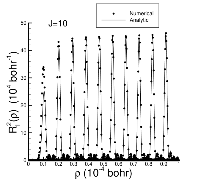
Figure 1: The $R_{i}^{2}(\rho)$ DV wavefunctions for J=10 and N=40 with $\rho_{0}=10^{-4}\ bohr.$ The numerical wavefunctions are calculated by diagonalizing the potential matrix $\Phi_{nm}$ in (27) and the analytic wavefunctions are found from (28) and (29). For clarity, only every fourth wavefunction is shown.

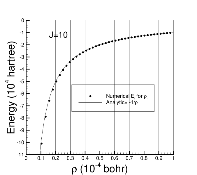
Figure 2: The numerical energies $E_{i}$ are found by diagonalizing the potential matrix $\Phi_{nm}$ in (27) with J=10 and N=40. The $\rho_{i}$ are zeros of $j_{10}(k_{41}\rho)$.

III.2 Magnetic Potential

Using the Coulomb potential $\Phi_{C}(\rho)=-e^{2}/\rho$ in (1) for the DV states, one obtains the energies $E_{i}=-e^{2}/\rho$ for all four $\Psi_{DV}$ in (37). However, one still needs to include the appropriate magnetic potential $\Phi_{M}$ so that the total Coulomb potential $\Phi$ is then

$$\Phi\mathbf{=}\Phi_{C}+\Phi_{M}.$$ (39)

The appropriate magnetic potential will depend on the gauge used. While, in theory, results should be gauge independent, in practice, different bases have different QED convergence characteristics which make some gauge choices impractical.

For the atomic positronium states where $k<<m$, one finds that the expectation value of the Dirac operators $\left\langle\boldsymbol{\alpha}_{e}\right\rangle=-\left\langle\boldsymbol{\alpha}_{p}\right\rangle$ is of order $\alpha=e^{2}/\hbar c\sim 1/137$. Here the weak-weak to strong-strong component ratio $\Psi_{22}/\Psi_{11}$ is of order $\alpha^{4}.$ For the atomic calculations, it is most convenient to use the Coulomb gauge with the Breit magnetic potential $\Phi_{B}$ (derived from second order perturbation theory), so that

$$\Phi_{B} =\frac{e^{2}}{2\rho}[\boldsymbol{\alpha}_{e}\cdot\boldsymbol{\alpha}_{p}+\left(\boldsymbol{\alpha}_{e}\cdot\widehat{\boldsymbol{\rho}}\right)\left(\boldsymbol{\alpha}_{p}\cdot\widehat{\boldsymbol{\rho}}\right)],$$

$$\Phi_{Atom} =\Phi_{C}+\Phi_{B}=\Phi_{C}\{1-\frac{1}{2}[\boldsymbol{\alpha}_{e}\cdot\boldsymbol{\alpha}_{p}+\left(\boldsymbol{\alpha}_{e}\cdot\widehat{\boldsymbol{\rho}}\right)\left(\boldsymbol{\alpha}_{p}\cdot\widehat{\boldsymbol{\rho}}\right)]\},$$

which results in fine structure corrections to the Coulomb energies for positronium. Using this magnetic potential and the Pauli approximation restriction to a $\Psi_{++}$ bases, the fine structure energies for positronium have been found analytically to order $m\alpha^{4}$ by Ferrell Ferrell (1951), Bethe and Salpeter (1957). Also, Fulton and Martin Fulton and Martin (1954) have used the BSE for the $\Psi_{Atom}$ bases with various two-body QED kernels in addition to the Coulomb potential to calculate the energies of positronium to order $m\alpha^{5}$. In agreement with the BSE (21), they found it necessary to omit the $\Psi_{+-}$ and $\Psi_{-+}$ anomalous states. Also, unlike the TBDE, it is necessary to use the negative of the Coulomb potential $-\Phi_{C}$ in $\Lambda_{Atom}$ for the negative energy states $\Psi_{--}$.

For the DV positronium states in (37), where $m<<k$, one finds that the expectation value of the Dirac operators $\left\langle\boldsymbol{\alpha}_{e}\right\rangle=\left\langle\boldsymbol{\alpha}_{p}\right\rangle\rightarrow 1$ when $\left\langle\mathcal{M}\right\rangle\rightarrow 0$ in (6) and the components $\Psi_{11}$ and $\Psi_{22}$ are equal in magnitude as shown in (37). Because of these extremely relativistic states, QED covariant perturbation theory is not convergent and diagonalization of the potential is necessary. Indeed, one finds that the expectation values of the magnetic and electromagnetic potentials become comparable in magnitude as in the classical case for highly relativistic particles. Accordingly, one must use the DV potential $\Phi_{DV}$ with the instantaneous magnetic potential of Gaunt $\Phi_{G}$ Alstine and Crater (1997), so that

$$\Phi_{G} =\frac{e^{2}}{\rho}\boldsymbol{\alpha}_{e}\cdot\boldsymbol{\alpha}_{p}\equiv\frac{e^{2}}{\rho}(\alpha_{ex}\alpha_{px}+\alpha_{ey}\alpha_{py}+\alpha_{ez}\alpha_{pz}),$$ (40)

$$\Phi_{DV} =\Phi_{C}+\Phi_{G}=\Phi_{C}\alpha_{0}^{2},$$

$$\alpha_{0}^{2} =(1-\boldsymbol{\alpha}_{e}\cdot\boldsymbol{\alpha}_{p}).$$

This total potential has also been derived by Barut and Komy Barut and Komy (1985) using the action principal. The operator $\boldsymbol{\alpha}_{e}\cdot\boldsymbol{\alpha}_{p}$ only acts on the Pauli- and Dirac-spinors of $\Psi_{DV}$ in (37) and it is shown below that the DV states are eigenstates of $\alpha_{0}^{2}$ in (40) as well as the potential $\Phi_{C}$. Barut and Komy have shown that this instantaneous effective potential is appropriate for the retarded propagator $K_{R}$ which is the propagator used for the DV states in (22). As described in the Appendix, the DV potential $\Phi_{DV}=\Phi_{C}\alpha_{0}^{2}$ is related to the Lorentz potential

$$\Phi_{L}=\Phi_{C}\gamma_{0}^{2},$$ (41)

where $\gamma_{0}^{2}=$ $\gamma_{eu}\gamma_{pu}$ is the scalar product of $\gamma_{eu}$ and $\gamma_{pu}$. The correct potential for the BSE equation in (22), which uses the $K_{R}$ propagator, should be multiplied on the left by the factor $\alpha_{0}^{2}$.

One can evaluate the Pauli-spinor operator $\boldsymbol{\sigma}_{e}\cdot\boldsymbol{\sigma}_{p}$ in the magnetic potential for states in (37) using

$$(\boldsymbol{\sigma}_{e}\cdot\boldsymbol{\sigma}_{p})\Omega_{0}^{0} =-3\Omega_{0}^{0},$$ (42)

$$(\boldsymbol{\sigma}_{e}\cdot\boldsymbol{\sigma}_{p})\Omega_{S_{z}}^{1} =\Omega_{S_{z}}^{1},$$

for $S_{z}=-1,0,1$. Evaluating the operator $\boldsymbol{\alpha}_{e}\cdot\boldsymbol{\alpha}_{p}$ for Dirac- and Pauli-spinor states gives

$$(\boldsymbol{\alpha}_{e}\cdot\boldsymbol{\alpha}_{p})(\mathbf{e}_{11}\pm\mathbf{e}_{22})\Omega_{0}^{0} =\mp 3(\mathbf{e}_{11}\pm\mathbf{e}_{22})\Omega_{0}^{0},$$ (43)

$$(\boldsymbol{\alpha}_{e}\cdot\boldsymbol{\alpha}_{p})(\mathbf{e}_{12}\pm\mathbf{e}_{21})\Omega_{0}^{0} =\mp 3(\mathbf{e}_{12}\pm\mathbf{e}_{21})\Omega_{0}^{0},$$

$$(\boldsymbol{\alpha}_{e}\cdot\boldsymbol{\alpha}_{p})(\mathbf{e}_{11}\pm\mathbf{e}_{22})\Omega_{S_{z}}^{1} =\pm(\mathbf{e}_{11}\pm\mathbf{e}_{22})\Omega_{S_{z}}^{1},$$

$$(\boldsymbol{\alpha}_{e}\cdot\boldsymbol{\alpha}_{p})(\mathbf{e}_{12}\pm\mathbf{e}_{21})\Omega_{S_{z}}^{1} =\pm(\mathbf{e}_{11}\pm\mathbf{e}_{22})\Omega_{S_{z}}^{1},$$

so that these spinor states are all eigenfunctions of $\boldsymbol{\alpha}_{e}\cdot\boldsymbol{\alpha}_{p}$. For the DV states in (37), one then finds

$$\Phi_{DV}|\Psi^{0},J\rho_{i}\rangle =E_{i}^{0}|\Psi^{0},J\rho_{i}\rangle,$$ (44)

$$E_{i}^{0} =M_{i}^{0}=2e^{2}/\rho_{i},$$

$$\Phi_{DV}|\Psi^{1},J\rho_{i}\rangle =E_{i}^{1}|\Psi^{1},J\rho_{i}\rangle,$$

$$E_{i}^{1} =M_{i}^{1}=0.$$

These DV eigenstates of $\Phi_{DV}$ no longer have negative energies and are, therefore, physically allowed.

One can divide the magnetic Gaunt potential into its longitudinal and transverse components,

$$\Phi_{G}=\Phi_{GL}+\Phi_{GT},$$ (45)

where

$$\Phi_{GL}=\frac{e^{2}}{\rho}(\alpha_{ez}\alpha_{pz}),\ \ \ \Phi_{GT}=\frac{e^{2}}{\rho}(\alpha_{ex}\alpha_{px}+\alpha_{ey}\alpha_{py}).$$ (46)

Interestingly, one has for all DV states in (37),

$$\alpha_{ez}\alpha_{pz}|\Psi,J\rho_{i}\rangle=|\Psi,J\rho_{i}\rangle,$$ (47)

so that

$$(\Phi_{C}+\Phi_{GL})|\Psi,J\rho_{i}\rangle =0,$$ (48)

$$\Phi_{DV}|\Psi,J\rho_{i}\rangle =\Phi_{GT}|\Psi,J\rho_{i}\rangle.$$

This means that, for the DV bound-states, only the transverse magnetic potential $\Phi_{GT}$ of Gaunt determines the energies in (44). On the other hand, for the atomic states, it is the Coulomb potential which is dominant.

Summarizing, the DV states $|\Psi^{0},J\rho_{i}\rangle$ for $\Omega_{0}^{0}$ form ‘heavy’ doublets with energy $E_{i}^{0}=2e^{2}/\rho_{i}$ and the DV states $|\Psi^{1},J\rho_{i}\rangle$ for $\Omega_{+}^{1}$ form ‘light’ doublets with $E_{i}^{1}=0$. The four degenerate states in (37) with Coulomb energies $E_{i}=-e^{2}/\rho_{i}$ are now split by the magnetic potential into two different doublets.

IV Classical Correspondence

For clarity, the constant $c$ is now shown in this section. The different behaviors between the atomic and anomalous states all depend on the fact that, for anomalous states, either the electron or positron is in a negative energy state $\psi_{-}(e)$ or $\psi_{-}(p)$, respectively. It is possible to understand the important properties of the DV states by using both quantum and classical principals. In particular, it is now shown that the four anomalous bound-states $\Psi_{DV}$ are both stable and dark, as was the case for the $J=0$ bound-states in Patterson (2019).

For a free-particle with energy $E=\pm\left|E\right|$ and momentum $\mathbf{p}$, one obtains the important result Sakurai (1967) for the expectation value of the Dirac matrices $\alpha_{k}$,

$$\left\langle\alpha_{k}\right\rangle=p_{k}c/E=\pm p_{k}c/\left|E\right|=v_{k}/c.$$ (49)

In other words, the velocity $\mathbf{v}$ is in the direction opposite to the momentum $\mathbf{p}$ for negative energy states of free-particles. In the $P^{\prime}$$=\mathbf{0}$ frame, where $\mathbf{p}_{e}=-\mathbf{p}_{p}$, one finds that $\mathbf{v}_{e}=\mathbf{v}_{p}$ because either the electron or the positron is in a negative energy state. The difference in velocity components is then

$$\left\langle(\boldsymbol{\alpha}_{e}-\boldsymbol{\alpha}_{p})_{k}\right\rangle=0\mathbf{.}$$ (50)

One can now understand why kinetic energy $\left\langle K\right\rangle$ is zero in (29) despite the fact that the relativistic momentum $\pi$ is large, $\pi=k>>mc$. One has

$$\left\langle K\right\rangle =c\left\langle(\boldsymbol{\alpha}_{e}-\boldsymbol{\alpha}_{p})\cdot\mathbf{\pi}\right\rangle,$$

$$=c\left\langle(\boldsymbol{\alpha}_{e}-\boldsymbol{\alpha}_{p})_{k}\right\rangle\left\langle\mathbf{\pi}_{k}\right\rangle=0.$$

Classically, (49) corresponds to $m=-\left|m\right|$ when $E=-\left|E\right|$ and for $\mathbf{p}_{e}=-\mathbf{p}_{p}$ one also finds that $\mathbf{v}_{e}=\mathbf{v}_{p}$ for both the anomalous states $\Psi_{+-}$ or $\Psi_{-+}$.

With this in mind, one can also understand why the DV states are delta functions with $\Psi_{DV}=G\delta(\rho-\rho_{i})$. From the Heisenberg uncertainty principal, these delta functions correspond to very high momentum states where $\pi>>mc$. Because the relative velocity is zero, $\mathbf{v}_{e}-\mathbf{v}_{p}=0$, the classical particles will remain at the same arbitrary distance $\rho=\rho_{i}$. Also, the electron and positron particles can never annihilate because they can never collide. Finally, two particles moving at the same velocity can neither radiate nor absorb light. This later property is also clear from quantum considerations, given that the expectation value of the Dirac transition operator $\mathbf{W}_{\mu}$ is

$$\left\langle\mathbf{W}_{\mu}\right\rangle=-e\left\langle(\boldsymbol{\alpha}_{e}-\boldsymbol{\alpha}_{p})\cdot\mathbf{1}_{\mu}\right\rangle=0,$$ (51)

where $\mu=z$ for longitudinal and $\mu=x,y$ for transverse radiation.

It is also apparent that an electron and positron moving with the same velocity can keep the same time so that one may let $t_{e}=t_{p}=t$. For this reason, there will be no difficulties with the DV solutions of the BSE in (22) that arise from the particles keeping different times. The total time $T$ is the fourth component of $\mathbf{R}$ in (5) and is conjugate to the total energy $E$. One sees that the total time $T$ and the relative time $t$ are the same,

$$T=\frac{t_{e}+t_{p}}{2}=t.$$ (52)

In many respects, the solutions to the BSE (22) for anomalous bound-states $\Psi_{DV}$ are simpler than the solutions to the BSE (21) for the atomic states $\Psi_{Atom}$.

Finally, one can readily determine the classical instantaneous electromagnetic interaction between electron and positron point particles with angular momentum $J\neq 0$.  One finds the magnetic force $F_{M}$ is

$$F_{M}=-\frac{e^{2}}{\rho^{2}c^{2}}[\mathbf{v}_{e}\times(\mathbf{v}_{p}\times\widehat{\boldsymbol{\rho}})]$$ (53)

for velocities $v\ll c$. In the center of mass frame with $\mathbf{R}=0$, let the classical velocities be perpendicular to $\mathbf{r}_{e}=\boldsymbol{\rho}/2$ and $\mathbf{r}_{p}=-\boldsymbol{\rho}/2$ for $J\neq 0$ so that

$$[\mathbf{v}_{e}\times(\mathbf{v}_{p}\times\widehat{\boldsymbol{\rho}})]=(\mathbf{v}_{e}\cdot\widehat{\boldsymbol{\rho}})\mathbf{v}_{p}-\mathbf{(v}_{e}\mathbf{\cdot v}_{p}\mathbf{)}\widehat{\boldsymbol{\rho}}=-\mathbf{(v}_{e}\mathbf{\cdot v}_{p}\mathbf{)}\widehat{\boldsymbol{\rho}},$$

and

$$F_{M}=\frac{e^{2}}{\rho^{2}c^{2}}\mathbf{(v}_{e}\mathbf{\cdot v}_{p}\mathbf{)}\widehat{\boldsymbol{\rho}}.$$ (54)

One finds that the force $F_{M}$ is repulsive in the $\widehat{\boldsymbol{\rho}}$ direction for the electron and positron moving in the same direction as required. The electromagnetic potential for $J\neq 0$ is then

$$\Phi=\Phi_{C}+\Phi_{M}=-\frac{e^{2}}{\rho}(1-\frac{\mathbf{v}_{e}\mathbf{\cdot v}_{p}}{c^{2}}\mathbf{).}$$ (55)

For relativistic velocities, the retarded Lienard-Wiechert potential preserves the ratio $\Phi_{C}/\Phi_{M}=-\mathbf{v}_{e}\mathbf{\cdot v}_{p}/c^{2}$. Letting $\mathbf{v}_{e}=\mathbf{v}_{p}=\mathbf{c}$ where $\Phi_{C}/\Phi_{M}=-1$, the classical and quantum potential is then $\Phi=0$ as in (44) for the $S=1$ case. Note that the quantum potential (40) can be derived from (55) by replacing $\mathbf{v}_{e}\mathbf{\cdot v}_{p}/c^{2}$ with $\boldsymbol{\alpha}_{e}\cdot\boldsymbol{\alpha}_{p}$. This quantum potential $\Phi_{DV}=\Phi_{C}\alpha_{0}^{2}$ is valid for all velocities and is in agreement with Barut and Komy Barut and Komy (1985) using the retarded $K_{R}$ propagator. It’s transformation to a moving frame is shown in the Appendix.

V Lorentz Boosts, Dynamical Symmetry Breaking, and Majorana Fermions

Consider a new frame in which the DV states are moving with velocity $V^{\prime}$ in the $Z$ direction so that the DV states have total momentum $P^{\prime}=P_{Z}^{\prime}$ relative to the rest frame. One can also, without loss of generality, define the $z$ direction to be in the direction of this momentum so that the components of spins $s_{z}$ will be defined in the $\widehat{\mathbf{z}}=\widehat{\mathbf{Z}}$ direction.

One can transform the DV states $\Psi_{i}$ and potential $\Phi_{DV}=\Phi_{C}\alpha_{0}^{2}$ (40) to the moving frame using both the two-body Lorentz boost $L^{2}$ of the Dirac spinors and the Lorentz contraction of the $z$ coordinate. In the Appendix, some useful identities (89) and (92) for the conjugate expectations of $\alpha_{0}^{2}$, $\Phi_{C}\alpha_{0}^{2}$, and $\Phi_{C}^{\prime}\alpha_{0}^{2}$ are

$$\left\langle\Psi_{i}\left|\alpha_{0}^{2}\right|\Psi_{i}\right\rangle =\left\langle\Psi_{i}^{\prime}\left|\alpha_{0}^{2}\right|\Psi_{i}^{\prime}\right\rangle,$$ (56)

$$\langle\Psi_{i}|\Phi_{C}\alpha_{0}^{2}|\Psi_{i}\rangle =M_{i},$$

$$\langle\Psi_{i}^{\prime}|\Phi_{C}^{\prime}\alpha_{0}^{2}|\Psi_{i}^{\prime}\rangle =M_{i}^{\prime},$$

where $M_{i}$ is the binding energy of $\Psi_{i}$ in the rest frame and $M_{i}^{\prime}$ is the binding energy of $\Psi_{i}^{\prime}$ in the moving frame. Only if this binding energy remains constant, such that $M_{i}^{\prime}=M_{i}$, can one demonstrate that the DV states transform like single-particle fermions. As shown below, the mass $M_{i}^{\prime}$ is a constant in the moving frame for all $\Psi_{i}^{\prime 1}$ DV states in (37), but only for a special case of the DV states $\Psi_{i}^{\prime 0}$ which corresponds to the lowest energy state.

The Lorentz boost has the properties

$$\Psi^{\prime} =L^{2}\Psi,\ \Phi_{DV}^{\prime}=L^{2}\Phi_{DV}L^{-2},\qquad$$ (57)

$$L^{-2} =\gamma_{4}^{2}L^{2}\gamma_{4}^{2},\ \ \ \gamma_{4}^{2}=\gamma_{e4}\gamma_{p4},\$$

where $L^{-2}$ is the inverse transform of $L^{2}$. These transformations involve some difficulties arising from dynamical symmetry breaking and the fact that $L^{2}$ is not unitary, which are now addressed.

As shown by (37) and (38), the DV wavefunctions $\Psi_{i}^{0}$ and $\Psi_{i}^{1}$ for a given $J$ can be separated into two factors. One factor consist only of the Dirac spinors $\Omega_{S_{z}}^{S}\mathbf{e}_{ij}$ and the other factor consists only of the coordinate functions $\Delta_{i}(\rho,\theta)$. The Lorentz boost operates on the Dirac spinors $\Omega_{S_{z}}^{S}\mathbf{e}_{ij}$, whereas the Lorentz contraction operates on the functions $\Delta_{i}(\rho,\theta)$. Similarly, for the potential $\Phi_{DV}$, the Lorentz boost operates on the factor $\alpha_{0}^{2}$ and the Lorentz contraction operates on the factor $\Phi_{C}=-e^{2}/\rho$. The Lorentz contraction of $\rho$ in $\Delta_{i}(\rho,\theta)$ and $\Phi_{C}$ will be considered first.

Because of the delta function factor $\delta(\rho-\rho_{i})$ (38), the  $\Delta_{i}(\rho,\theta)$ in the rest frame are eigenstates of $1/\rho$ in $\Phi_{C}$ such that

$$\frac{1}{\rho}\Delta_{i}(\rho,\theta)=\frac{1}{\rho_{i}}\Delta_{i}(\rho,\theta).$$ (58)

However, as a result of the Lorentz contraction of $z_{i}$ in the potential, $z_{i}^{\prime}=z_{i}/\gamma$, the separations $\rho_{i}^{\prime}$ are no longer spherically symmetric. Because of this dynamical symmetry breaking, the potential $\Phi_{C}$ becomes cylindrically symmetric and $\rho_{i}^{\prime}$ depends on $\theta_{i}^{\prime}$. This means that $\Delta_{i}^{\prime}(\rho^{\prime},\theta^{\prime})$ is no longer an eigenstate of the $1/\rho^{\prime}$. This problem can be remedied by using delta functions $\delta(\cos\theta-\cos\theta_{i})$ in $\Delta_{i}$ formed from the degenerate $P_{0}^{J}(\cos\theta)$ and $P_{1}^{J}(\cos\theta)$ in (38) without any effect on the energies $E_{i}$. Letting $\zeta=\cos\theta$, the delta functions for the DV states directed at angle $\theta=\theta_{i}$ are given by

$$\left\{\begin{array}[c]{c}[\delta(\zeta-\zeta_{i})+\delta(\zeta+\zeta_{i})\ \text{ }J=even\\ [\delta(\zeta-\zeta_{i})-\delta(\zeta+\zeta_{i})\ \text{ }J=odd\end{array}\right\} ={\textstyle\sum\limits_{J}}(2J+1)P_{0}^{J}(\zeta_{i})P_{0}^{J}(\zeta),$$ (61)

$$\left\{\begin{array}[c]{c}[\delta(\zeta-\zeta_{i})+\delta(\zeta+\zeta_{i})\ \text{ }J=odd\\ [\delta(\zeta-\zeta_{i})-\delta(\zeta+\zeta_{i})\ \text{ }J=even\end{array}\right\} ={\textstyle\sum\limits_{J}}\frac{2J+1}{J(J+1)}P_{1}^{J}(\zeta_{i})P_{1}^{J}(\zeta).$$ (64)

One must keep in mind that the peaks of the delta functions $\zeta_{i}$ are not the same for the symmetric and antisymmetric delta functions above because the peaks of $P_{0}^{J}(\zeta_{i})$ are interleaved for $J=even$ and $J=odd$ and similarly for $P_{1}^{J}(\zeta_{i})$. For example, the symmetric delta functions can have a peak at $\zeta_{i}=0$ whereas the antisymmetric delta functions cannot. This means that when $\zeta_{i}=0$, the $\Psi_{i}^{0}$ DV state has $J=even$ and the $\Psi_{i}^{1}$ DV state has $J=odd$. In (38), one now has, approximately,

$$\Delta_{i}^{0} \simeq D_{i}^{0}\delta(\rho-\rho_{i})[\delta(\zeta-\zeta_{i})\pm\delta(\zeta+\zeta_{i})]/\sqrt{4\pi},$$ (65)

$$\Delta_{i}^{1} \simeq D_{i}^{1}\delta(\rho-\rho_{i})[\delta(\zeta-\zeta_{i})\pm\delta(\zeta+\zeta_{i})]/\sqrt{4\pi,}$$

from (61). These new functions $\Delta_{i}$ are localized at the coordinates $(\rho_{i},\theta_{i})$ and remain eigenstates of $1/\rho$ (58) because $\rho$ is independent of $\theta$.

For a given velocity $V^{\prime}$ with the Lorentz factor $\gamma$, one has the following relations for the Lorentz contraction of $z$, using the cylindrical coordinates $(r_{i},z_{i})$,

$$\rho_{i}^{\prime}\cos\theta_{i}^{\prime} =z_{i}^{\prime}=z_{i}/\gamma=\rho_{i}\cos\theta_{i}/\gamma,$$

$$\rho_{i}^{\prime}\sin\theta_{i}^{\prime} =r_{i}^{\prime}=r_{i}=\rho_{i}\sin\theta_{i}.$$

Solving these equations, one finds

$$\rho_{i}^{\prime} =(\rho_{i}/\gamma)\sqrt{\gamma^{2}-\cos^{2}(\theta_{i})(\gamma^{2}-1)},$$ (66)

$$\cos\theta_{i}^{\prime} =\rho_{i}\cos\theta_{i}/(\rho_{i}^{\prime}\gamma).$$

The new factors $\Delta_{i}^{\prime}$ for $\Psi_{i}^{\prime}$, resulting from the Lorentz contraction, are then simply

$$\Delta_{i}^{0\prime} \simeq D_{i}^{0\prime}\delta(\rho^{\prime}-\rho_{i}^{\prime})[\delta(\zeta^{\prime}-\zeta_{i}^{\prime})\pm\delta(\zeta^{\prime}+\zeta_{i}^{\prime})]/\sqrt{4\pi},$$ (67)

$$\Delta_{i}^{1\prime} \simeq D_{i}^{1\prime}\delta(\rho^{\prime}-\rho_{i}^{\prime})[\delta(\zeta^{\prime}-\zeta_{i}^{\prime})\pm\delta(\zeta^{\prime}+\zeta_{i}^{\prime})]/\sqrt{4\pi},$$

for DV states localized at coordinates $(\rho_{i}^{\prime},\theta_{i}^{\prime})$ given by (66) where $\zeta_{i}^{\prime}=\cos\theta_{i}^{\prime}$. With this simple procedure, the factors $\Delta_{i}^{\prime}$ for $\Psi_{i}^{\prime}$ are now eigenstates of $1/\rho^{\prime}$

$$\frac{1}{\rho^{\prime}}\Delta_{i}^{\prime}(\rho^{\prime},\theta^{\prime})=\frac{1}{\rho_{i}^{\prime}}\Delta_{i}^{\prime}(\rho^{\prime},\theta^{\prime}).$$ (68)

Now consider the Lorentz boost of $K,$ $\Phi_{DV}$, and the DV states $\Psi_{i}$. In the Appendix it is shown, using adjoint spinors, that

$$\langle\Psi_{i}^{0\prime}|K^{\prime}|\Psi_{i}^{0\prime}\rangle=0,$$

so the transformed wavefunctions are also DV states. For the potential, one can also verify from (44), (56), and (68) that

$$\langle\Psi_{i}^{0\prime}|\Phi_{C}^{\prime}\alpha_{0}^{2}|\Psi_{i}^{0\prime}\rangle =M_{i}^{0\prime}=2e^{2}/\rho_{i}^{\prime},$$ (69)

$$\langle\Psi_{i}^{1\prime}|\Phi_{C}^{\prime}\alpha_{0}^{2}|\Psi_{i}^{1\prime}\rangle =M_{i}^{1\prime}=0.$$

For the $\Psi_{i}^{1\prime}$ DV states, one has $M_{i}^{1\prime}=M_{i}^{1}=0$ so that $\beta^{\prime}=1$ and the velocity $V^{\prime}$ will be the speed of light. For these light DV states, one has $\gamma^{\prime}\rightarrow\infty$ and $z_{i}^{\prime}=0$ such that $\rho_{i}^{\prime}=\rho_{i}=r_{i}$ and they form a disk perpendicular to the direction of motion $\mathbf{\hat{z}=}\widehat{\mathbf{Z}}$. In this case the potential expectation value $\left\langle\Phi_{DV}\right\rangle$ is a Lorentz invariant as required for these DV states to transform like a single-particle fermion.

For the $\Psi_{i}^{0\prime}$ DV states, one has $M_{i}^{0\prime}=2e^{2}/\rho_{i}^{\prime}\neq M_{i}^{0}$ when $z_{i}\neq 0$ and the masses are not Lorentz invariant. In fact one finds from (66), for a given $\rho_{i}$, that $M_{i}^{0\prime}$ is a maximum when $\theta_{i}=0$ or $\theta_{i}=\pi$ where $\rho_{i}^{\prime}=\rho_{i}/\gamma$ and $M_{i}^{0\prime}=\gamma M_{i}^{0}$. One also finds from (66), for a given $\rho_{i}$, that $M_{i}^{0\prime}$ is a minimum when $\theta_{i}=\pi/2$ $(z_{i}=0)$ where $\rho_{i}^{\prime}=\rho_{i}$ and $M_{i}^{0\prime}=M_{i}^{0}$. In general one finds that

$$\gamma M_{i}^{0}\geq M_{i}^{0\prime}\geq M_{i}^{0}$$

for a given $\rho_{i}$. This is a consequence of the fact that, for a given $\rho_{i},$ the Lorentz contraction will bring the electron and positron closer together for any angle $\theta_{i}$ unless $\theta_{i}=\pi/2$. Because the potential is repulsive, this will then raise the binding energy and mass $M_{i}^{0\prime}$ unless $\theta_{i}=\pi/2$. For the special case where $\theta_{i}=\pi/2$ $(z_{i}=0),$ the DV states $\Psi_{i}^{0\prime}$ form a disk perpendicular to the direction of motion $\mathbf{\hat{z}=}\widehat{\mathbf{Z}}$ such like the DV states $\Psi_{i}^{1\prime}$. One would expect that this particle would reside in the lowest energy DV state of $\Psi_{i}^{0\prime}$ with $\theta_{i}=\pi/2$, where the mass is invariant. The fact that such DV doublets $\Psi_{i}$ with $M_{i}^{0\prime}=M_{i}^{0}$ transform like single-particle fermions will now be shown.

Having transformed the coordinate factors $\Delta_{i}(\rho,\theta)$ for the DV states $\Psi_{i}^{0}$ and $\Psi_{i}^{1}$ for $J=(even,odd)$ as shown in (67), it remains to transform their Dirac spinors $\Omega_{S_{z}}^{S}\mathbf{e}_{ij}$ to the frame moving with velocity $V^{\prime}$. Brodsky and Primack Brodsky and Primack (1969) have shown, using the BSE for atomic hydrogen, that the Lorentz boost for $P^{\prime}$ mixes the four different Pauli-spinors $\Omega_{S_{z}}^{S}$ among themselves and the four different Dirac-spinors $\mathbf{e}_{ij}$ among themselves. The Lorentz boost for a single-particle fermion in the $z$ direction with velocity $\left\langle\alpha_{z}^{\prime}\right\rangle=V^{\prime}$ is

$$L=\sqrt{\frac{\gamma^{\prime}+1}{2}}\mathbf{+}\sqrt{\frac{\gamma^{\prime}-1}{2}}\alpha_{z}^{\prime}.$$ (70)

For the DV states (37), with $\Delta_{i}$ given (65), including the plane-wave function $f$, the box-normalized wavefunction in the rest frame is

$$|\Psi,J\rho_{i}\rangle f=|\Psi,J\rho_{i}\rangle e^{-iM_{i}T}/\sqrt{Z_{0}}.$$

One can boost the DV state with velocity $V^{\prime}\$so that the total momentum is $P^{\prime}$. The two-body Lorentz boost $L^{2}$ is the direct product of the Lorentz boosts $L_{e}\times L_{p}$ such that

$$L^{2}=L_{e}\times L_{p}=\left(\sqrt{\frac{\gamma+1}{2}}\mathbf{+}\sqrt{\frac{\gamma-1}{2}}\alpha_{ez}\right)\times\left(\sqrt{\frac{\gamma+1}{2}}\mathbf{+}\sqrt{\frac{\gamma-1}{2}}\alpha_{pz}\right),$$

where $\gamma$ corresponds to the individual particle boosts $\pm\beta$. Letting $\sqrt{\gamma^{2}-1}=\beta\gamma$ and using (47) when operating on the DV states, one has

$$L^{2} =\frac{\gamma+1}{2}+\frac{\gamma-1}{2}\alpha_{ez}\alpha_{pz}+\beta\gamma\frac{(\alpha_{ez}+\alpha_{pz})}{2},$$ (71)

$$=\gamma\mathbf{+}\beta\gamma\alpha_{z}^{\prime},$$

where

$$\alpha_{z}^{\prime}=\frac{(\alpha_{ez}+\alpha_{pz})}{2},$$ (72)

as in (6). In the frame where $\mathbf{\pi}=\mathbf{0}$, one has $\mathbf{p}_{e}=\mathbf{p}_{p}$ so that the velocity of the electron and positron are equal and opposite, $\mathbf{v}_{e}=-\mathbf{v}_{p}$, where either the electron or the positron is in a negative energy state. Transforming to either the electron or positron frame, one can add these velocities relativistically, so that

$$V^{\prime}=\beta^{\prime}=\pm 2\beta/(1+\beta^{2}).$$

Then the two-body Lorentz boost (71) is equivalent to

$$L^{2}=\sqrt{\frac{\gamma^{\prime}+1}{2}}\mathbf{+}\sqrt{\frac{\gamma^{\prime}-1}{2}}\alpha_{z}^{\prime},$$ (73)

where

$$\gamma^{\prime}=(1-\beta^{{}^{\prime}2})^{-\frac{1}{2}}=(1+\beta^{2})/(1-\beta^{2}).$$

But this is just the boost (70) with velocity $V^{\prime}=\beta^{\prime}$ where the rest mass is now $M_{i}^{\prime}$ in (69) such that

$$V^{\prime} =\beta^{\prime}=P^{\prime}/E_{i}^{\prime},$$ (74)

$$E_{i}^{\prime} =\sqrt{P^{\prime 2}+M_{i}^{\prime 2}},\ \ \gamma^{\prime}=E_{i}^{\prime}/M_{i}^{\prime},\ \ \ \beta^{\prime}\gamma^{\prime}=P^{\prime}/M_{i}^{\prime}.$$

In general, because $\rho_{i}^{\prime}\neq\rho_{i}$, the binding energy has changed in the moving frame so that $M_{i}^{\prime}\neq M_{i}$ and the particle cannot be considered a single-particle fermion.

One can now use $L^{2}$ in (73) to transform the DV states in (37) with $\Delta_{i}$ in (65) and confirm the results above in (69). Operating with $\alpha_{ez}$ and $\alpha_{pz}$ in (72), one finds that

$$\alpha_{ez}\Omega_{0}^{0}(\mathbf{e}_{11}-\mathbf{e}_{22}) =\alpha_{pz}\Omega_{0}^{0}(\mathbf{e}_{11}-\mathbf{e}_{22})=-\Omega_{0}^{1}(\mathbf{e}_{12}-\mathbf{e}_{21}),$$ (75)

$$\alpha_{ez}\Omega_{0}^{0}(\mathbf{e}_{12}-\mathbf{e}_{21}) =\alpha_{pz}\Omega_{0}^{0}(\mathbf{e}_{12}-\mathbf{e}_{21})=-\Omega_{0}^{1}(\mathbf{e}_{11}-\mathbf{e}_{22}),$$

$$\alpha_{ez}\Omega_{+}^{1}(\mathbf{e}_{11}+\mathbf{e}_{22}) =\alpha_{pz}\Omega_{+}^{1}(\mathbf{e}_{11}+\mathbf{e}_{22})=-\Omega_{-}^{1}(\mathbf{e}_{12}+\mathbf{e}_{21}),$$

$$\alpha_{ez}\Omega_{+}^{1}(\mathbf{e}_{12}+\mathbf{e}_{21}) =\alpha_{pz}\Omega_{+}^{1}(\mathbf{e}_{12}+\mathbf{e}_{21})=-\Omega_{-}^{1}(\mathbf{e}_{11}+\mathbf{e}_{22}),$$

(and their Hermitian conjugates) so that

$$\alpha_{z}^{\prime}|\Psi,J\rho_{i}\rangle=\alpha_{ez}|\Psi,J\rho_{i}\rangle=\alpha_{pz}|\Psi,J\rho_{i}\rangle.$$ (76)

The transformed wavefunctions $\Psi_{i}^{\prime}$, after renormalization, are

$$\Psi_{i,A}^{0\prime} =\frac{1}{2}\Delta_{i}^{0\prime}\left\{\sqrt{\gamma^{\prime}+1}\Omega_{0}^{0}(\mathbf{e}_{11}-\mathbf{e}_{22})-\sqrt{\gamma^{\prime}-1}\Omega_{0}^{1}(\mathbf{e}_{12}-\mathbf{e}_{21})\right\}/\sqrt{\gamma^{\prime}},$$ (77)

$$\Psi_{i,S}^{0\prime} =\frac{1}{2}\Delta_{i}^{0\prime}\left\{\sqrt{\gamma^{\prime}+1}\Omega_{0}^{0}(\mathbf{e}_{12}-\mathbf{e}_{21})-\sqrt{\gamma^{\prime}-1)}\Omega_{0}^{1}(\mathbf{e}_{11}-\mathbf{e}_{22})\right\}/\sqrt{\gamma^{\prime}},$$

$$\Psi_{i,1S}^{1\prime} =\frac{1}{2}\Delta_{i}^{1\prime}\{\Omega_{+}^{1}(\mathbf{e}_{11}+\mathbf{e}_{22})-\Omega_{-}^{1}(\mathbf{e}_{12}+\mathbf{e}_{21})\},$$

$$\Psi_{i,2S}^{1\prime} =\frac{1}{2}\Delta_{i}^{1\prime}\{\Omega_{+}^{1}(\mathbf{e}_{12}+\mathbf{e}_{21})-\Omega_{-}^{1}(\mathbf{e}_{11}+\mathbf{e}_{22})\},$$

where the $\Delta_{i}^{\prime}$ are given by (67). The renormalization factor $\sqrt{1/\gamma^{\prime}}$ comes from the Lorentz contraction $Z_{0}^{\prime}=Z_{0}/\gamma^{\prime}$ of the transformed plane-wavefunction,

$$\ f^{\prime}=e^{i(P^{\prime}Z^{\prime}-E_{i}^{\prime}T^{\prime})}/\sqrt{Z_{0}^{\prime}}.\$$ (78)

Using (44) and (6.20), one can readily verify (69). One can also verify directly that the DV states in (77) are solutions to the one-body Dirac equation (6),

$$(\alpha_{z}^{\prime}P_{Z}^{\prime}+M^{\prime}\gamma_{4}^{2})f^{\prime}|\Psi_{i}^{\prime}\rangle=E_{i}^{\prime}f^{\prime}|\Psi_{i}^{\prime}\rangle,$$ (79)

where $M^{\prime}\gamma_{4}^{2}=\Phi_{C}^{\prime}\alpha_{0}^{2}$ and $E_{i}^{\prime}=\sqrt{P_{Z}^{\prime}+(M_{i}^{\prime})^{2}}$ as shown in the Appendix. To confirm that the DV states with $z_{i}=0$ are single-particle fermions, one has $\rho^{\prime}=\rho$ and $\Phi_{C}^{\prime}=\Phi_{C}$ for these special DV states, so that $M^{\prime}=M$.

For these ‘pancake’ wavefunctions with $z_{i}=z_{i}^{\prime}=0$, the DV states for $S_{z}=\pm 1$ and $S_{z}=0$ then transform like fermion doublets in which the Lorentz contraction in $z$ has no effect. Looking more closely at the spinor states of (77), one finds that, instead of the expected single-particle doublet Pauli-spinors $(\chi_{\frac{1}{2}},\chi_{-\frac{1}{2}})$, one now has the doublet Dirac-spinors $\left\{(\mathbf{e}_{11}-\mathbf{e}_{22}),(\mathbf{e}_{12}-\mathbf{e}_{21})\right\}$ for $\Psi^{0\prime}$ and $\left\{(\mathbf{e}_{11}+\mathbf{e}_{22}),(\mathbf{e}_{12}+\mathbf{e}_{21})\right\}$ for $\Psi^{1\prime}$, respectively. Also, one finds that, instead of the expected single-particle Dirac-spinors $(\mathbf{e}_{1},\mathbf{e}_{2})$, one now has the Pauli-spinors $(\Omega_{0}^{0},\Omega_{0}^{1})$ for $\Psi^{0\prime}$ and $(\Omega_{+}^{1},\Omega_{-}^{1})$ for $\Psi^{1\prime}$. For a given DV bound-state doublet, the spin states $s_{z}(e)$ and $s_{z}(p)$ are completely correlated and act like a single-particle spin state $s_{z}$. That is, for the Pauli-spinors $(\Omega_{0}^{0},\Omega_{0}^{1})$, one has $s_{z}(e)=-s_{z}(p)$, whereas for the Pauli-spinors $(\Omega_{+}^{1},\Omega_{-}^{1})$, one has $s_{z}(e)=s_{z}(p)$.

Summarizing, the directed DV doublets with coordinates $r=r_{i}$ and $z_{i}=0$ in the rest frame transform like a single-particle fermion when undergoing a Lorentz boost because of dynamical symmetry breaking. The rest mass for the heavy fermions is $M_{i}^{0\prime}=M_{i}^{0}=2e^{2}/r_{i}$ and rest mass for the light fermions is $M_{i}^{1\prime}=M_{i}^{1}=0$. As shown by (61) for $z_{i}=0$, the $\Psi^{0\prime}$ DV states must have $J=even$ and the $\Psi^{1\prime}$ DV states must have $J=odd$. However, for both of these fermions, the role of Pauli-spinors and Dirac-spinors has been reversed because either the electron or positron is in a negative energy state. The $S_{z}=0$ fermions in (77) have both $S$ and $A$ symmetry under exchange whereas the $S_{z}=\pm 1$ fermions have only $A$ symmetry. Most importantly, because these DV states are comprised of either $S$ or $A$ symmetry, they are their own antiparticles and the light and heavy DV doublets are Majorana fermions.

VI Chirality $\chi$ and Helicity $h$ of the Light Fermions

The light DV fermions $\Psi_{i}^{1\prime}=\Psi_{i,A}^{1\prime}$ with $z_{i}=0$ in (77) have $A$ exchange symmetry for $J=odd$ corresponding to the symmetric delta functions in $\Delta_{i,S}^{1\prime}$ (67) and the $e^{\pm i\phi}$ dependence in (36). These $\Psi_{i}^{1\prime}$ DV states have well defined chirality and helicity because the rest mass is $M_{i}^{1\prime}=0$. The chirality operator $\boldsymbol{\chi}=-\gamma_{5}$ for a single-particle operates on the Dirac-spinors such that, for any $i=1,2,$

$$\boldsymbol{\chi}_{e}\mathbf{e}_{1i}=\mathbf{e}_{2i},\ \boldsymbol{\chi}_{p}\mathbf{e}_{i1}=\mathbf{e}_{i2},$$

and their Hermitian conjugates. When operating on these DV states in (77), one can define the chirality operator $\boldsymbol{\chi}^{\prime}$ as

$$\boldsymbol{\chi}^{\prime}=\frac{(\boldsymbol{\chi}_{e}+\boldsymbol{\chi}_{p})}{2},$$ (80)

where $\boldsymbol{\chi}^{\prime}\Psi_{i}^{1\prime}=\boldsymbol{\chi}_{e}\Psi_{i}^{1\prime}=\boldsymbol{\chi}_{p}\Psi_{i}^{1\prime}$ .

The helicity operator $\mathbf{h}=\mathbf{\Sigma\cdot}\widehat{\mathbf{P}^{\prime}}=\mathbf{\Sigma}_{z}$ for a single-particle operates on the Pauli-spinors such that

$$\mathbf{h}_{e}\Omega_{1}^{1} =\Omega_{1}^{1},\ \mathbf{h}_{e}\Omega_{-1}^{1}=-\Omega_{-1}^{1},$$

$$\ \mathbf{h}_{p}\Omega_{1}^{1} =\Omega_{1}^{1},\ \mathbf{h}_{p}\Omega_{-1}^{1}=-\Omega_{-1}^{1}.$$

Again, when operating on the DV states (77), one can define the helicity operator $\mathbf{h}^{\prime}$ for the light fermions as

$$\mathbf{h}^{\prime}=\frac{(\mathbf{h}_{e}+\mathbf{h}_{p})}{2},$$ (81)

where $\mathbf{h}^{\prime}\Psi_{i}^{1\prime}=\mathbf{h}_{e}\Psi_{i}^{1\prime}=\mathbf{h}_{p}\Psi_{i}^{1\prime}$.

The eigenfunctions of both $\boldsymbol{\chi}^{\prime}$ and $\mathbf{h}^{\prime}$ are then

$$\Psi_{i,+}^{1\prime} =(\Psi_{i,1A}^{1\prime}+\Psi_{i,2A}^{1\prime})/\sqrt{2}$$ (82)

$$=\frac{1}{2}\Delta_{i,S}^{1\prime}\{(\mathbf{e}_{11}+\mathbf{e}_{22}+\mathbf{e}_{12}+\mathbf{e}_{21})\Omega_{1}^{1}e^{-i\phi}\},$$

$$\Psi_{i,-}^{1\prime} =(\Psi_{i,1A}^{1\prime}-\Psi_{i,2A}^{1\prime})/\sqrt{2}$$

$$=\frac{1}{2}\Delta_{i,S}^{1\prime}\{(\mathbf{e}_{11}+\mathbf{e}_{22}-\mathbf{e}_{12}-\mathbf{e}_{21})\Omega_{-1}^{1}e^{i\phi}\},$$

such that $\boldsymbol{\chi}^{\prime}\Psi_{i,\pm}^{1\prime}=\chi^{\prime}\Psi_{i,\pm}^{1\prime}$ and $\mathbf{h}^{\prime}\Psi_{i,\pm}^{1\prime}=h^{\prime}\Psi_{i,\pm}^{1\prime}$. These states $\Psi_{i,\pm}^{1\prime}$ have chirality $\chi^{\prime}=\pm 1$ and helicity $h^{\prime}=\pm 1$, respectively, corresponding to right- and left-handed chirality and to right- and left-handed helicity. As in the case of a single-particle fermion with no mass, the chirality and helicity of these light DV Majorana fermions have the same signs.

VII Conclusions

It has been shown that the solutions of the Bethe-Salpeter equation (BSE) for the atomic bound-states of positronium in (21) and for the anomalous bound-states of positronium in (22), result in two entirely different forms of positronium. One is the normal atomic form of positronium in which the electron and positron are bound at atomic distances ($bohr$), and the other is the anomalous form of positronium in which the particles can be bound at nuclear distances ($fermi$). Such anomalous bound-states are called discrete variable (DV) states because they form a bases for the DV representation in which the relative coordinates $(\rho,\theta)$ between the electron and positron are quantized at discrete values $(\rho_{i},\theta_{i})$. For the atomic states, the BSE stipulates that the negative energy states must propagate backward in time with $K_{F}$, whereas, for the DV states, the BSE stipulates that the negative energy states must propagate forward in time with $K_{R}$. For the DV states, only bound-state solutions are allowed because of the time behavior of the negative energy states, and these bound-states cannot dissociate.

It has also been shown that the properties of the anomalous bound-states and the atomic bound-states differ radically because, for the former, either the electron or the positron must be in a negative energy state. It is instructive to compare and contrast the properties of the atomic and DV bound-state solutions for positronium, as they are complementary. The atomic bound-states in the rest frame have low relative momentum $\pi<<m$, and can be treated using the Coulomb gauge, whereas the DV bound-states in the rest frame have very high relative momentum $\pi>>m$ and must be treated relativistically with the Feynman gauge. For the atomic free-states, there is no potential energy and the momenta are quantized. For the DV bound-states, there is no relative kinetic energy and the relative coordinates are quantized. The atomic states are bound mainly by the Coulomb potential whereas the DV bound-states are bound only by the transverse magnetic potential. The atomic states of positronium are unstable and decay quickly into photons, whereas the DV states of positronium are stable and cannot decay. Also, the atomic states can emit and absorb light, whereas the DV states are dark.

The atomic states of positronium are bosons with total spin $S=1$ (corresponding to the triplets $\Omega_{-1}^{1},\Omega_{0}^{1},\Omega_{1}^{1}$) and $S=0$ (corresponding to the singlet $\Omega_{0}^{0}$). The DV states of positronium are comprised of $S_{z}=0$ doublets $(\Omega_{0}^{0},\Omega_{0}^{1})$ which have opposite spins $s_{z}(e)=-s_{z}(p)$, and $S_{z}=\pm 1$ doublets $(\Omega_{1}^{1},\Omega_{-1}^{1})$ which have aligned spins $s_{z}(e)=s_{z}(p)$. In both these cases the individual electron and positron spins are correlated and transform like single-particle fermions by a Lorentz boost when they are in the plane perpendicular to the direction of motion.

The fermion nature of the DV states occurs because the wavefunctions are Lorentz contracted in the direction of motion $\widehat{z}$ resulting in the spherical symmetry being reduced to cylindrical symmetry. The relative coordinates $(r,z)$ can then be quantized in the $z=0$ plane with $r=r_{i}$. For such states the binding energy is independent of the motion and the DV doublet states behave like single-particle fermions. The $S_{z}=0$ fermions for $(\Omega_{0}^{0},\Omega_{0}^{1})$ are heavy particles with mass $M_{i}^{0}=2e^{2}/r_{i}$ and the $S_{z}=\pm 1$ fermions for $(\Omega_{-1}^{1},\Omega_{1}^{1})$ are light particles with mass $M_{i}^{1}=0$. Because the DV fermions are either symmetric $\Psi_{S}=\sqrt{\frac{1}{2}}(\Psi_{+-}+\Psi_{-+})$ or antisymmetric $\Psi_{A}=\sqrt{\frac{1}{2}}(\Psi_{+-}-\Psi_{-+})$, depending on their angular momentum $J$, they are their own antiparticle and are therefore Majorana fermions. However, for the light fermions, which can only occur in the $z=0$ plane, only the $\Psi_{A}$ states are possible. They also have well defined helicity and chirality because their mass $M_{i}$ is zero. Thus, the solutions of the BSE equation for positronium result in two forms of matter with contrasting but complementary characteristics.

It does not appear that the DV states are relevant, per se, to atomic physics. The question arises as to whether there are any particles which have the properties of the DV bound-state fermions. It appears that the properties of the DV fermions are consistent with those of light and heavy neutrinos. One can then hypothesize that the DV states corresponding to the $S_{z}=\pm 1$ light fermions are electron neutrinos and the DV states corresponding to the $S_{z}=0$ heavy fermions are ‘sterile’ neutrinos. The ‘sterile’ type of neutrino has been surmised by some particle physicists as an explanation for dark matter Boyarsky et al. (2019). The sterile neutrino would then have a mass of $\sim MeV$ if the electron and positron were bound at nuclear distances ($fermi$). The fact that these DV bound-states are Majorana fermions and are not single point particles would then explain the violation of parity and charge conjugation by the weak force. These light Majorana fermions can have either left- or right-handed helicity (with the same chirality) which is then, presumably, selected by the weak force to give the observed handedness of neutrinos.

The fact that these light and heavy Majorana fermions are dark, stable, and are composed of equal amounts of matter (electrons) and antimatter (positrons) could then simultaneously explain both the apparent absence of antimatter in the universe as well as the apparent presence of dark matter. Further investigation of this hypothesis is necessary to show that the light fermions have other properties of the electron neutrinos besides the ones shown here. One needs to show that the light fermions have the measured weak force cross-sections and are consistent with the proven theory of vector bosons.

Appendix A Lorentz Boost of Operators Using Adjoint and Conjugate Spinors

Operator equations using the Lorentz boost $L^{2}$ involve difficulties because $L^{2}$ is not a unitary transform. The Lorentz boosts of wavefunction $\Psi$ and operator $O$ comprised of Dirac spinors have the properties

$$\Psi^{\prime} =L^{2}\Psi,\ O^{\prime}=L^{2}OL^{-2},\qquad$$ (83)

$$L^{-2} =\gamma_{4}^{2}L^{2}\gamma_{4}^{2},\ \ \ \gamma_{4}^{2}=\gamma_{e4}\gamma_{p4},\$$

where $L^{-2}$ is the inverse transform. Define the adjoint spinor to be

$$\langle\overline{\Psi}| =\left\langle\Psi\right|\gamma_{4}^{2},$$ (84)

$$\langle\overline{\Psi^{\prime}}| =\left\langle\Psi^{\prime}\right|\gamma_{4}^{2}=\left\langle\Psi\right|L^{2}\gamma_{4}^{2}=\left\langle\Psi\right|\gamma_{4}^{2}\gamma_{4}^{2}L^{2}\gamma_{4}^{2}=\left\langle\overline{\Psi}\right|L^{-2},$$

where $\left\langle\Psi\right|$ is the conjugate spinor. There are two different expressions for the expectation value of an operator $O$ which is Lorentz boosted. Define the adjoint expectation of operator $O$ to be $\langle\overline{\Psi}\left|O\right|\Psi\rangle$ and the conjugate expectation to be $\left\langle\Psi\left|O\right|\Psi\right\rangle$. The adjoint expectation of $O$ is a Lorentz invariant,

$$\langle\overline{\Psi^{\prime}}\left|O^{\prime}\right|\Psi^{\prime}\rangle=\left\langle\overline{\Psi}\left|O\right|\Psi\right\rangle$$ (85)

which for $O=1$ corresponds to the Lorentz scalar,

$$\langle\overline{\Psi^{\prime}}|\Psi^{\prime}\rangle=\langle\overline{\Psi}|\Psi\rangle.$$

This invariant form of the expectation should be used when transforming to the moving frame. For example, using (85) for the kinetic operator $K$, one finds that, for the DV states,

$$\langle\overline{\Psi^{\prime}}\left|K^{\prime}\right|\Psi^{\prime}\rangle=\left\langle\overline{\Psi}\left|K\right|\Psi\right\rangle=0,$$ (86)

so that the transformed wavefunctions in (37) are still anomalous states with zero kinetic energy.

The DV potential can be written

$$\Phi_{DV}=-\frac{e^{2}}{\rho}(1-\boldsymbol{\alpha}_{e}\cdot\boldsymbol{\alpha}_{p})=\Phi_{C}\alpha_{0}^{2},$$

where $\Phi_{C}$ is the Coulomb potential. The operators $\alpha_{0}^{2}$ and $\gamma_{4}^{2}$ commute so that $\alpha_{0}^{2}\gamma_{4}^{2}=\gamma_{4}^{2}\alpha_{0}^{2}$. To find the transform properties of the DV potential, one must consider the Lorentz invariant operator $\gamma_{0}^{2}=\gamma_{eu}\gamma_{pu}$, which is the scalar product of the two four-vectors $\gamma_{eu}$ and $\gamma_{pu}$. This scalar operator transforms such that

$$\gamma_{0}^{\prime 2}=\gamma_{eu}^{\prime}\gamma_{pu}^{\prime}=\gamma_{eu}\gamma_{pu}=\gamma_{0}^{2},$$ (87)

or equivalently,

$$\gamma_{0}^{\prime 2}=\gamma_{4}^{\prime 2}\alpha_{0}^{\prime 2}=\gamma_{4}^{2}\alpha_{0}^{2}=\gamma_{0}^{2}.$$ (88)

Unlike the operator $\gamma_{0}^{2}$, the operator $\alpha_{0}^{2}$ is not a Lorentz invariant as seen in (88). From the above equations one finds that

$$\left\langle\overline{\Psi}\left|\gamma_{0}^{2}\right|\Psi\right\rangle =\left\langle\overline{\Psi}\left|\gamma_{4}^{2}\alpha_{0}^{2}\right|\Psi\right\rangle=\left\langle\Psi\left|\alpha_{0}^{2}\right|\Psi\right\rangle,$$

$$\langle\overline{\Psi^{\prime}}\left|\gamma_{0}^{\prime 2}\right|\Psi^{\prime}\rangle =\langle\overline{\Psi^{\prime}}\left|\gamma_{4}^{2}\alpha_{0}^{2}\right|\Psi^{\prime}\rangle=\left\langle\Psi^{\prime}\left|\alpha_{0}^{2}\right|\Psi^{\prime}\right\rangle.$$

Letting $\left\langle\overline{\Psi}\left|\gamma_{0}^{2}\right|\Psi\right\rangle=\langle\overline{\Psi^{\prime}}\left|\gamma_{0}^{\prime 2}\right|\Psi^{\prime}\rangle$, one finds the useful result

$$\left\langle\Psi\left|\alpha_{0}^{2}\right|\Psi\right\rangle=\left\langle\Psi^{\prime}\left|\alpha_{0}^{2}\right|\Psi^{\prime}\right\rangle.$$ (89)

The instantaneous Lorentz potential $\Phi_{L}$ is given by

$$\Phi_{L}=\Phi_{C}\gamma_{0}^{2}=\gamma_{4}^{2}\Phi_{DV}.$$

This potential $\Phi_{L}$ can be derived in the momentum representation from the invariant potential used by Salpeter Salpeter (1952),

$$G(k_{u}) =-e^{2}(\gamma_{0}^{2}/k_{0}^{2}),$$

$$k_{0}^{2} =\mathbf{k\cdot k-\varpi}^{2}.$$

For the instantaneous Lorentz potential in the momentum representation, let $\mathbf{\varpi}^{2}=0$. Now let the two-body mass operator for the DV states be defined by

$$M\gamma_{4}^{2}=\Phi_{L}\gamma_{4}^{2}=\Phi_{C}\alpha_{0}^{2}=\Phi_{DV},$$ (90)

so that the two-body mass operator is the analogy of the one-body mass operator $m\gamma_{4}.$ One must then use the two-body mass operator,

$$M^{\prime}\gamma_{4}^{2}=\Phi_{L}^{\prime}\gamma_{4}^{2}=\Phi_{C}^{\prime}\alpha_{0}^{2},$$ (91)

when finding the mass $M^{\prime}$ in the moving frame in analogy with the one-body case.

From (90) and (91), one finds that the adjoint expectation of the Lorentz potential $\Phi_{L}$ and $\Phi_{L}^{\prime}$ is

$$M =\left\langle\overline{\Psi}\left|\Phi_{L}\right|\Psi\right\rangle=\left\langle\Psi|\Phi_{C}\alpha_{0}^{2}|\Psi\right\rangle,$$ (92)

$$M^{\prime} =\langle\overline{\Psi^{\prime}}\left|\Phi_{L}^{\prime}\right|\Psi^{\prime}\rangle=\left\langle\Psi^{\prime}|\Phi_{C}^{\prime}\alpha_{0}^{2}|\Psi^{\prime}\right\rangle.$$

The Lorentz potential is a Lorentz invariant when $\rho^{\prime}=\rho$ or when $\Phi_{C}^{\prime}=\Phi_{C}$. Combining the result (89) with the Lorentz contraction of $\rho$ to $\rho^{\prime}$ in the moving frame allows one to find $M$ and $M^{\prime}$ in (92). Using $M$ in (92) and (58) confirms (44). Using $M^{\prime}$ in (92) and (68) confirms (69), where

$$M_{i}^{0\prime} =\langle\Psi_{i}^{0\prime}|\Phi_{C}^{\prime}\alpha_{0}^{2}|\Psi_{i}^{0\prime}\rangle=2e^{2}/\rho_{i}^{\prime},$$ (93)

$$M_{i}^{1\prime} =\langle\Psi_{i}^{1\prime}|\Phi_{C}^{\prime}\alpha_{0}^{2}|\Psi_{i}^{1\prime}\rangle=0.$$

This results in the two-body equation for the DV states in the moving frame

$$(\alpha_{z}^{\prime}P_{Z}^{\prime}+M^{\prime}\gamma_{4}^{2})f^{\prime}|\Psi_{i}^{\prime}\rangle =E_{i}^{\prime}f^{\prime}|\Psi_{i}^{\prime}\rangle,$$ (94)

$$\ f^{\prime} =e^{i(P^{\prime}Z^{\prime}-E_{i}^{\prime}T^{\prime})}/\sqrt{Z_{0}^{\prime}}.$$

as in (79). This equation is equivalent to the single-body Dirac equation for a fermion only if $M^{\prime}=M$ such that the rest mass is constant in the moving frame.

References

• Scott et al. (1992) T. C. Scott, J. Shertzer, and R. A. Moore, Phys. Rev. A 45, 4393 (1992).
• Patterson (2019) C. W. Patterson, Phys. Rev. A 100, 062128 (2019).
• Light and Carrington (2000) J. C. Light and T. Carrington, Adv. Chem. Phys. 114, 263 (2000).
• Salpeter and Bethe (1951) E. E. Salpeter and H. A. Bethe, Phys. Rev. 84, 1232 (1951).
• Salpeter (1952) E. E. Salpeter, Phys. Rev. 87, 328 (1952).
• Malenfant (1988) J. Malenfant, Phys. Rev. D 38, 3295 (1988).
• Feynman (1949) R. P. Feynman, Phys. Rev. 76, 749 (1949).
• Abramowitz and Stegun (1972) M. Abramowitz and I. A. Stegun, Handbook of Mathematical Functions (Dover Publishing, New York, 1972).
• Ferrell (1951) R. A. Ferrell, Phys. Rev. 84, 858 (1951).
• Bethe and Salpeter (1957) H. A. Bethe and E. E. Salpeter, Quantum Mechanics of One- and Two-Electron Atoms (Academic Press, New York, 1957).
• Fulton and Martin (1954) T. Fulton and P. C. Martin, Phys. Rev. 95, 811 (1954).
• Alstine and Crater (1997) P. V. Alstine and H. W. Crater, Found. Phys. 27, 67 (1997).
• Barut and Komy (1985) A. O. Barut and S. Komy, Fortschritte der Physik 33, 309 (1985).
• Sakurai (1967) J. J. Sakurai, Advanced Quantum Mechanics (Addison-Wesley, New York, 1967).
• Brodsky and Primack (1969) S. J. Brodsky and J. R. Primack, Annals of Physics 52, 315 (1969).
• Boyarsky et al. (2019) A. Boyarsky, M. Drewes, T. Lasserre, S. Merten, and O. Ruchayskiy, Prog. Part. Nucl. Phys. 104, 1 (2019).