The relation between Parisi scheme and multi-thermalized dynamics in finite dimensions

Abstract

In this note we summarize the connections between equilibrium and slow out of equilibrium dynamics in finite dimensional glasses, such as we understand them today. If we assume that a finite-dimensional system is stable with respect to a family of weak random perturbations (stochastic stability), then its dynamics have a ‘Multithermalization’ structure if and only if the Boltzmann-Gibbs distribution obeys an Ultrametric Parisi distribution.

I Introduction

A system whose equilibrium measure follows the Parisi scheme Mézard et al. (1987), commonly known as Replica Symmetry Breaking (RSB), will take an infinite time to reach its equilibrium starting form random configurations, a process called ‘aging’. It may also be driven into an out of equilibrium steady-state by an infinitesimal drive, such as shear Thalmann (2001); Berthier et al. (2000a), or time-dependence of disorder Horner (1992). If the relaxation times are long, or, in a steady-state if the drive is weak, the dynamics are slow: this is the regime we are interested in.

The out of equilibrium dynamics under these circumstances is a very specific one Sompolinsky and Zippelius (1982, 1981); Horner (1992); Cugliandolo and Kurchan (1993, 1994); Franz and Mézard (1994). At given times one may define an effective temperature with a thermodynamic meaning Cugliandolo et al. (1997), it is the same for all observables. Different temperatures are possible, but in different ‘time scales’, a notion one has to define. We refer to this situation as ‘multithermalization’ Contucci et al. (2019, 2020).

In finite dimensional systems, neither the Parisi scheme nor the multi-thermalization scenario are proven to hold. However, the Parisi kind of ordering appears as the only possible non ergodic state which is stable against small random perturbations in the Hamiltonian.

Moreover, it turns out that Parisi RSB and multi-thermalization are deeply related: one of them holds if and only if the other also does. The temperatures involved in the slow dynamics then relate to the average overlap distribution computed for equilibrium in the Parisi scheme. This double implication may be argued on the basis of a strategy devised by Franz, Mézard, Parisi and Peliti (FMPP) Franz et al. (1998, 1999) and later generalized in Kurchan (2021) that uses linear response theory and equilibration of bulk quantities to compare dynamical quantities to equilibrium one. An extra element that is of central importance for the validity of both schemes, as we now realize, is the fact that the slow glassy dynamics is time-reparametrization soft: small perturbations dramatically stretch the timescales. Given the relation described above between static replica theory and slow dynamics, it is natural to search for reparametrization invariances in the Parisi replica context, and indeed questions like these have appeared in the literature. The whole matter deserves further clarification.

II Equilibrium: Ergodicity Breaking and the Parisi scheme

Replica Symmetry Breaking is ubiquitous in disordered systems with long range interactions Mézard et al. (1987). Its successful implementation by Giorgio Parisi dates back to the study of the Sherrington-Kirkpatrick model of a Spin Glass Sherrington and Kirkpatrick (1975), in the effort of parametrizing a $n\times n$ matrix for $n\to 0$ Parisi (1979). It describes the low temperature disordered frozen state with broken ergodicity in systems where ordinary ordering is not possible. For large samples, the Gibbs measure is dominated by a few ’valleys’ unrelated by symmetry and in random positions in configuration space. The distances between these valleys have broad distributions, but they are strongly constrained, in fact only isosceles triangles, with the different side the smallest are possible in the thermodynamic limit, the property of ‘ultrametricity’. The mathematical analysis of long range systems Talagrand et al. (2003); Panchenko (2013a) has fully confirmed and considerably enriched the picture coming from the physicist’s analysis based on the iconoclastic replica method and the more conventional, but still non rigorous Cavity Method. The Parisi picture is also a natural candidate to describe ideal thermodynamic glassy phases of systems with short range interactions. However, its validity in three and more in general in any finite dimensional systems has been seriously questioned Fisher and Huse (1986); Bray and Moore (1987). The best available numerical simulations give strong indications in favor of RSB above a critical dimension that is somewhere above two and below four.
The least one can say is that RSB provides a very good statistical description of samples of finite sizes, or, equivalently, of local properties of infinite samples. Local RSB has indeed been proven to hold in models with large but finite interaction range Franz and Toninelli (2004). But we do not know, with a convincing level of theoretical confidence, and even less of mathematical rigour, if RSB really survives as long range order in the thermodynamic limit. What indeed we know, is that under some rather mild assumption (see later), if random broken ergodicity holds, the structure of the probability measure on random Gibbs measures, also called metastate, should be qualitatively described by the RSB scenario. In fact, the mathematicians were able to prove that under the hypothesis that the overlap distributions verify the so called Ghirlanda-Guerra identities (GGI) Ghirlanda and Guerra (1998) then RSB ultrametric statistics follows Panchenko (2013b). In turn, the GGE follow from the stability of Gibbs measure against small perturbation Ghirlanda and Guerra (1998); Aizenman and Contucci (1998), an hypothesis that holds true in mean-field and, we will argue, can be generically accepted in finite dimension. Within Mean-Field, it soon appeared that the dynamics of RSB systems presents anomalies with respect to the one in ordinary ergodic systems Sompolinsky and Zippelius (1981, 1982). Recognizing the full fledged off-equilibrium character of these anomalies led to the surprise that aging phenomena, which are commonly observed in laboratory glasses, also appeared in mean-field models, giving rise to a coherent and detailed theory of dynamic ergodicity breaking Cugliandolo and Kurchan (1993, 1994). This is obtained by the asymptotic analysis of exact Dynamical Mean Field Theory (DMFT) equations, which display a low temperature solution violating basic equilibrium properties as time translation invariance and the relations between responses and correlation implied by the fluctuation dissipation theorem. It soon appeared that RSB and aging are intertwined phenomena in mean-field. Two classes of models were identified: p-spin like models and SK like models Cugliandolo and Kurchan (1993, 1994). In the former, one observes a decoupling between equilibrium and dynamics. The low temperature equilibrium measure is typically dominated by metastable states (ergodic components) with high stability, while the dynamics starting from a random configuration, tends to a marginal manifold which has higher energy density respect to the equilibrium states. In the latter, instead, the states dominating equilibrium are marginally stable, and the asymptotic dynamical solution predicts asymptotic values of extensive observables coinciding with the equilibrium ones. Unfortunately, the results of asymptotic dynamics have been rather elusive to rigorous mathematical analysis. While Parisi picture for equilibrium has been made fully rigurous by mathematicians, not much has been done in dynamics, where the only progress has been the proof of the validity of the physicist’s effective one body dynamical equations and their self-consistent Dynamical Mean Field Theory closure Arous and Guionnet (1995); Ben Arous et al. (2006). As far as finite dimension is concerned the situation is similar to the one of equilibrium: the Cugliandolo-Kurchan dynamical scenario provides an excellent description of finite time spin-glass dynamics Barrat and Kob (1999); Berthier et al. (1999), but we cannot exclude that the aging responses eventually become trivial and the system crosses over to complete thermalization.

II.1 Overlap Statistics

In the physics of the disordered systems in equilibrium a crucial role is played by the statistics of the overlap between replicas induced by the thermal and disorder fluctuations Mézard et al. (1987). What we call replicas here are configurations extracted independently from the Boltzmann measure for the same disorder. The overlap $Q[S,S^{\prime}]$ between two configurations is usually defined as $Q[S,S^{\prime}]=\frac{1}{N}\sum_{i=1}^{N}S_{i}S_{i}^{\prime}$.

A first characterization of the statistics of the overlap is given by its ’average histogram’

$$P(q)=\mathbb{E}\left(\langle\delta(Q[S_{1},S_{2}]-q))\rangle_{12}\right)$$ (1)

where we denoted as $\langle\cdot\rangle_{12}$ the average over the (product) Gibbs measure of the two replicas, and with $\mathbb{E}$ the average over their common disorder. It was shown by Parisi a long time ago, that a non trivial $P(q)$ (i.e. different from a single $\delta$ function) is associated to breakdown of ergodicity Parisi (1983). This is trivially true for example in systems with symmetry breaking in absence of a source, where it just reflects that the measure is uniform over the different possible phases of the system related to one another by symmetry. In that case, the function can be simply collapsed to a $\delta$ by the introduction of an infinitesimal symmetry-breaking source that selects one among the possible phases, and the function $P(q)$ does not play any physically important role in this case. In disordered systems $P(q)$ is not related to a any symmetry, and the situation can be much more interesting: a small perturbation unrelated to the original Hamiltonian cannot be expected to project on a single state, and modulo possible removal of accidental degeneracies of the original Hamiltonian, the function $P(q)$ of a perturbed system should stay close to the same function in the unperturbed one. This has deep consequences, since the multiplicity of states will affect the response properties of the system and $P(q)$ can be interpreted as the generating function of the responses to a family of random perturbations.

II.2 The method of random perturbations

The study of the overlap statistics requires access to microscopic configurations. This is of course easy in computer studies, but is more problematic in experiments. Fortunately one can use linear response theory (LRT) to give a different characterization of $P(q)$, as the generating function of a families of susceptibilities. Starting from a model with Hamiltonian $H$, one considers a perturbed system where random $p-spin$ like Hamiltonian are added to the energy of the system

$$H_{pert}[S]=H[S]+\sum_{p=1}^{\infty}\epsilon_{p}H_{p}[S]$$ (2)

where the perturbing terms are defined as

$$H_{p}[S]=-\sum_{i_{1},...,i_{p}}J_{i_{1},...,i_{p}}S_{i_{1}}...S_{i_{p}}$$ (3)

The couplings $J_{1_{i},...,i_{p}}$ are usually taken as centered i.i.d. Gaussian variables scaled as $\mathbb{E}\left(J_{1_{i},...,i_{p}}^{2}\right)=\frac{1}{N^{p-1}}$. If the parameters $\epsilon_{p}$ are chosen to be independent of $N$, the perturbing Hamiltonian involves extensive energy in equilibrium; it is straightforward to see that

$$I^{(p)}\equiv\frac{1}{N}\mathbb{E}[\langle H_{p}\rangle] = T\frac{\partial}{\partial\epsilon_{p}}\log Z=N\beta\epsilon_{p}(1-\langle q^{p}\rangle)$$ (4)

$$\langle q^{p}\rangle = \int dq\;P_{\epsilon}(q)q^{p}$$ (5)

that can be readily obtained by integration by parts. Values of $\epsilon_{p}$ vanishing with $N$, namely $\epsilon_{p}\sim N^{-a}$ with $0<a<1$, have also been considered, where (4) continues to hold, but the energy absorbed is sub-extensive. This suggests we define Stochastic Stability as the property that $P_{\epsilon}(q)\to P_{0}(q)$ (modulo symmetry or accidental degeneracy of the unperturbed Hamiltonian).

The reader may object that in an experimental system the susceptibilities defined by (4) are not more accessible than the microscopic configurations. The crucial point that we discuss later in the paper, however, is that, in turn, these quantities can be related to dynamical susceptibilities whose generator function can be in principle measured through response experiments in ageing dynamics.

II.3 Self-averageness and higher order overlap statistics

Higher order statistics of the overlaps, where one considers those between more than two replicas, are also important. Their distributions appears when formally considering the quadratic fluctuations of the perturbing terms $H_{p}$. For example, it is easy to show that the average square Hamiltonian $\mathbb{E}(\langle H_{p}[S]^{2}\rangle)$ is related to the statistics of two overlaps $P(q_{12},q_{13})$

$$\mathbb{E}(\langle H_{p}[S]^{2}\rangle)=\epsilon_{p}^{2}\beta^{2}N^{2}\left(1-2\langle q^{p}\rangle-\langle q^{2p}\rangle+\langle q_{12}^{p}q_{13}^{p}\rangle\right).$$ (6)

But $H$ is a self-averaging quantity, and at order $N^{2}$ $\mathbb{E}(\langle H_{p}[S]^{2}\rangle)=(\mathbb{E}(\langle H_{p}[S]\rangle))^{2}$. This implies a strong constraint on $P(q_{12},q_{13})$ which needs to verify

$$P(q_{13},q_{23})=\frac{1}{2}\delta(q_{13}-q_{23})P(q_{13})+\frac{1}{2}P(q_{12})P(q_{13}),$$ (7)

A similar analysis can be applied to $\mathbb{E}(\langle H_{p}[S]\rangle^{2})$, resulting in

$$P(q_{12},q_{34})=\frac{1}{3}\delta(q_{12}-q_{34})P(q_{12})+\frac{2}{3}P(q_{12})P(q_{34}).$$ (8)

Notice that $P(q_{12},q_{34})$ represents the average over disorder of the product of the disorder dependent overlap distribution of four independent replicas. Equation (8) tells us that this is different from $P(q_{12})P(q_{34})$: self-averageness of the energy, from which (8) is derived implies that the overlap probability (unless trivial) is instead non-self averaging. Also notice that once $P(q)$ is know, the higher order statistics of two overlaps are fixed.

II.4 Triangles

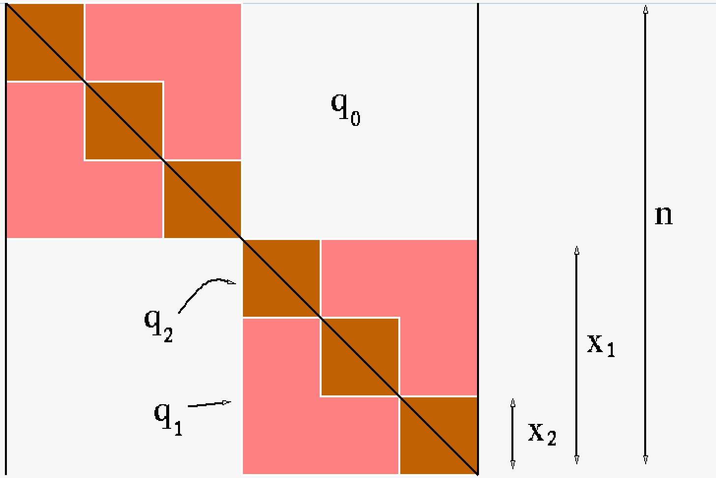
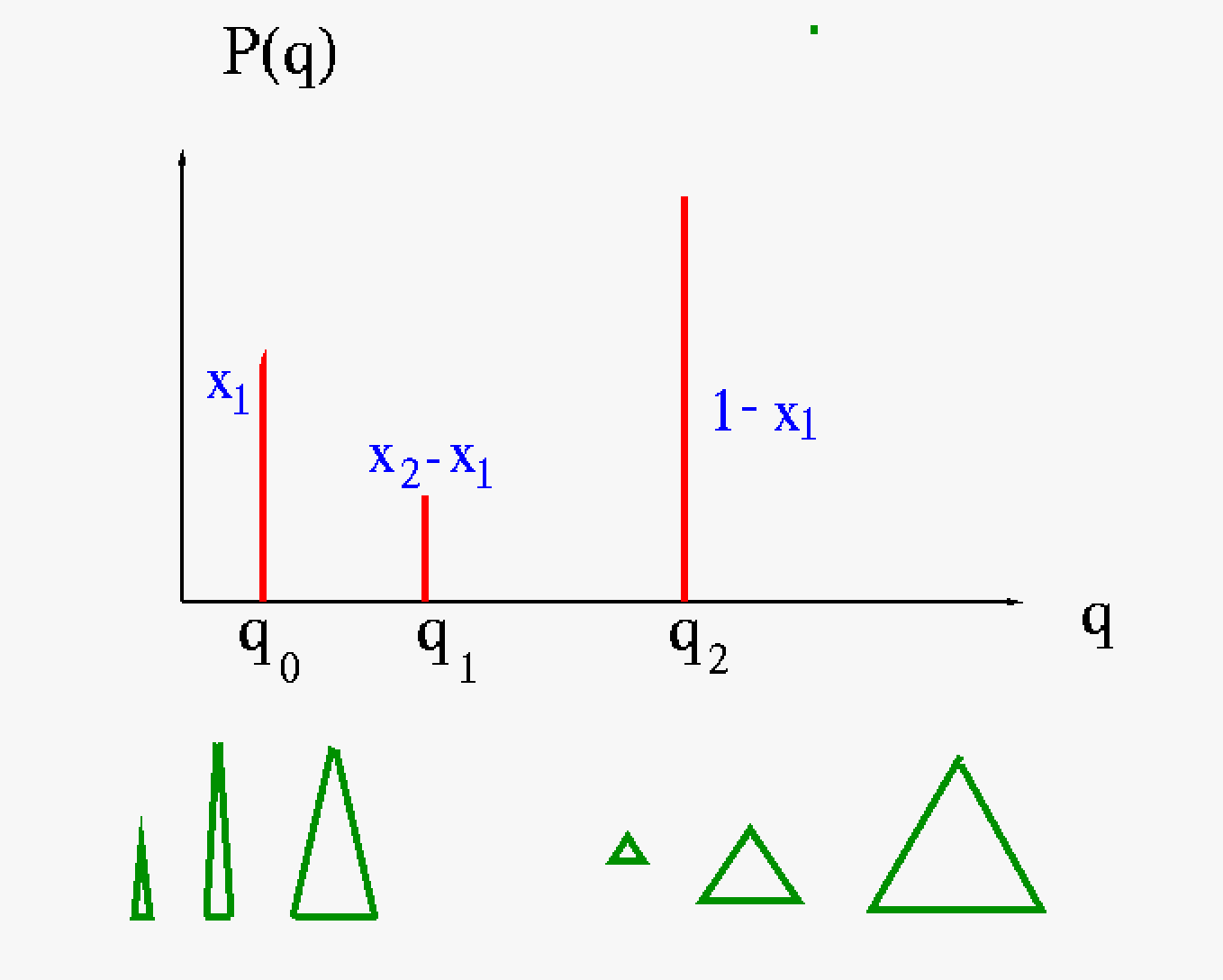
Equations (7,8) are examples of the celebrated Ghirlanda-Guerra identities Ghirlanda and Guerra (1998) that have played a crucial role in the mathematical analysis of Spin Glasses. It has been shown by Panchenko Panchenko (2013b) that in their most general form they imply ultrametricity (see Figs 1 and2) for any three states at mutual overlaps $q_{12},q_{23},q_{31}$: with probability one in the thermodynamic limit the two smallest overlaps are equal (all triangles are isosceles) $q_{13}=\min(q_{12};q_{23})$. Moreover, if we consider the conditional probability Mézard et al. (1987) we find:

$$P(q_{13}|q_{12}=q_{23}=q) = \frac{P(q_{13},q_{12}=q,q_{23}=q)}{P(q_{12}=q,q_{23}=q)}$$ (9)

$$= \theta(q_{13}-q)P(q_{13})+\delta(q_{13}-q)x(q).$$ (10)

where $x(q)=\int_{0}^{q}dq^{\prime}\;P(q^{\prime})$ is the cumulative probability. Notice that $q_{13}$ is independent of $q$ when it is larger than $q$, and that, as in the case of the overlap pairs, the triangle probabilities are fully specified by the function $P(q)$, or equivalently by its primitive, $x(q)$. Indeed, this generalizes to arbitrary number of replicas: thanks to self-averageness, $x(q)$ provides a sufficient statistics for the overlaps.

The picture is rather remarkable: in any system where extensive quantities are self-averaging and the system is stable with respect to small long-range random interactions, the only possibility besides triviality is ergodicity breaking according to the Parisi scheme. Originated in an unconventional mathematically analysis of the famous $0\times 0$ replica matrix, the Parisi RSB scheme has revealed a deep, and inescapable symmetry of nature, transcending the replica trick.

II.5 Overlap locking

It can be easily realized that if RSB is present in a system, then the overlap between any two random configurations should be homogeneous in space. This is true in long range systems, where by space we mean the complete graph (SK model) or the Bethe lattice (Viana-Bray model), but also, and especially, in any finite dimensional system with short range interaction that could possibly display RSB. Let us specifically refer to this case. Overlap homogeneity means that given two random equilibrium configurations, if one measures the value of the overlap in a given large enough region of space, the same value would be found by an analogous measure in any other region, no matter how far away from the original one. This is a very strong correlation property of equilibrium states.

Suppose you divide the system in two adjacent parts. The surface interaction term could be disconnected, without any appreciable change in the expectation values of bulk quantities. On the other hand, this term is crucial for the overlap statistics: in absence of the surface interaction the overlaps in the two halves are independent variables; in presence of it, the overlaps are locked to take the same values. We can generalize this consideration to more general weakly coupled disordered systems. The locking of the overlaps to identical values in the parts of the same system occurs because of statistical homogeneity of a given sample. An analogous locking however also occurs in absence of homogeneity, whenever we weakly couple systems with RSB. Suppose we have two systems ${\cal S}_{1}$ ${\cal S}_{2}$, whose overlap statistics is specified by $x_{1}(q)$ and $x_{2}(q)$ respectively, not necessarily identical. As before, as long as the systems are not interacting the overlaps are independent. Stability of the RSB state on the other hand requires that the as soon as a weak interaction is switched on, the overlaps do lock, and one can define a function $Q_{2}(q_{1})$, which allows to predict the overlap between two replicas in the system $S_{2}$, when the overlap is $q_{1}$ in the system $S_{1}$. It is clear that this relation should be specified by the condition $P_{1}(q_{1})dq_{1}=P_{2}(q_{2})dq_{2}$, or equivalently $x_{1}(q_{1})=x_{2}(Q_{2}(q_{1}))$ Franz et al. (1992). The actual functions $P_{1}(q)$ and $P_{2}(q)$ on the other hand will be only linearly affected by the coupling, and coincide in a fist approximation with the overlap probability distribution in the unperturbed systems. Here we encounter a first instance of ‘softness’ of the solution: the presence or absence of small, thermodynamically irrelevant terms, leads to a complete rearrangement of the Gibbs weights, without affecting the values of self-averaging quantities. Below we shall find the same property in the context of dynamics.

II.6 Marginal stability and Stochastic Stability in Mean-Field

Within mean-field, two classes of models are known: Models with ’full-RSB’, as the SK model, where the support $Supp(P)$ is a continuous interval, say $[q_{0},q_{1}]$ and models where the support has ’holes’. The most common case of this scenario is the case of ’one-step RSB’ (1RSB) where only two values of the overlap support the whole probability, this is the case of Potts-glasses and $p$-spin models and for simplicity we will refer to it here. We shall address these support values as ‘skeleton’ values of the correlations, and discuss how they play an important role in the correspondence between equilibrium and dynamics.

The physical picture between continuous and 1RSB cases is very different: in the first case the glassy phase is only marginally stable. This can be easily realized: the supports of the overlaps distributions are self-averaging Parisi and Talagrand (2004), implying that it is possible to go from a given state to any other crossing only sub-extensive barriers Franz and Parisi (1995, 1998). Within the replica method one finds families of Hessian zero modes associated to small variations $P(q)\to P(q)+\delta P(q)$ Temesvári et al. (2000); De Dominicis and Giardina (2006), a reparametrization transformation that has a deep dynamical analogue as we will see in the following sections. In the second case, conversely, equilibrium states are absolutely stable and are separated by extensive free-energy barriers. The effect of a small but extensive random perturbation is very different in the two cases. In the 1RSB cases the states are reshuffled: their weight changes but they keep their identity and continue to exist. In the full-RSB case the effect is more dramatic, any $O(N)$ perturbation destabilizes the unperturbed equilibrium states and produce new ones in random positions. A crucial property is that the probability distribution of the disorder-dependent Gibbs state is only affected in a regular way by the perturbation (i.e. linearly for small perturbations). This regularity property, called Stochastic Stability is very natural and at the same time important, it tells us that the original model is generic, sharing the same physics with a broad class of similar systems.

Figure 1: The famous Parisi hierarchical overlap matrix, encoding the full overlaps’ statistics of disordered systems with broken ergodicity.

Figure 2: The possible overlaps and the triangles they determine, according to the ultrametric ansatz.

III Dynamics and Multithermalization

III.1 Slow dynamics

In the dynamic approach we consider a system evolving according to local reversible dynamics. To fix the ideas we can consider the Langevin equation

$$-m_{i}{\ddot{s}}_{i}-\frac{\partial H({\bf s})}{\partial s_{i}}=\underbrace{\Gamma_{0}{\dot{s}}_{i}-\eta_{i}}_{bath}$$ (11)

where $\eta_{i}$ are uncorrelated Gaussian white noises with variance $2\Gamma_{0}T$ and $\Gamma_{0}$ is the strength of the coupling to the ‘white’ bath. This is guaranteed to reach eventually equilibrium, although in the systems that concern us, in times that may diverge with the system’s size $N$. For the considerations that follow, any stochastic reversible dynamics whose update rule just depends on the force $f_{i}=-\frac{\partial H({\bf s})}{\partial s_{i}}$ as e.g. Metropolis or Glauber dynamics would give rise to the same results. We shall be concerned with the limit of slow dynamics, which appears, in glassy systems, in different ways:

• Aging Castellani and Cavagna (2005): Following a quench of the system from a high to a low temperature, at which the equilibration time is infinite, the system ‘ages’: it evolves slower and slower as the time since the quench elapses. The two-time correlations never become an exclusive function of time-differences. The large parameter is the smallest ‘waiting’ time since the quench $t^{\prime}=t_{w}$, that modulates the decay at further time $C(t,t^{\prime})=C\left(\frac{\tau}{t_{w}}\right)$: the older (large $t_{w}$) the system, the slower the decay. In such conditions of long time scales local observables depending on configurations at a single time, such as the energy or specific heat, magnetization etc., only undergo small variations, and in what follows we will consider the ideal situation where they can be taken to be essentially equal to their asymptotic values.

• Driven system Thalmann (2001); Berthier et al. (2000a) When the system is subjected to forces not deriving from a potential – shear, for example – it is an experimental fact that aging is interrupted, in the sense that all functions become time-translational invariant, but slow. Their timescale of decay of correlation then is controlled by the driving rate $\sigma$, the slower the weaker the drive: $C(t-t^{\prime})=C\left({\tau}{\sigma}\right)$

• Time-dependent disorder Horner (1992). Another way to make a system with disorder time-translational invariant is to change the disorder slowly : the small parameter is the timescale $\tau_{0}$ of change of disorder: $C(t,t^{\prime})=C\left(\frac{\tau}{\tau_{0}}\right)$.

In what follows, we refer as slow dynamics to the limit of either long waiting times, small shear strains or slow variation of parameters. The latter two cases are stationary, all dependence on history is lost, but quite surprisingly they are not equilibrium systems, as we shall see.

In all these systems we consider correlation $C_{AB}(t,t^{\prime})$ and linear response function $R_{AB}(t,t^{\prime})$ (here $t\geq t^{\prime}$), the average response of $A$ at time $t$ to a kick of $B$ at time $t^{\prime}$. In the case of spin variables above, correlations and response functions are given by:

$$C_{ij}(t,t^{\prime})=\langle s_{i}(t)s_{j}(t^{\prime})\rangle\qquad;\qquad R_{ij}(t,t^{\prime})=\frac{\delta}{\delta h_{j}(t^{\prime})}\langle s_{i}(t)\rangle|_{h=0}$$ (12)

where $h_{i}(t)$ is the value at time $t$ of a field conjugated to $S_{i}$ in the Hamiltonian. One in general is interested to the global correlations and response, defined as $C(t,t^{\prime})=\frac{1}{N}\sum_{i}C_{ii}(t,t^{\prime})\qquad;\qquad R(t,t^{\prime})=\frac{1}{N}\sum_{i}R_{ii}(t,t^{\prime})$. It is useful to consider the response function in its integral form:

$$\chi(t,t^{\prime})=\int_{t^{\prime}}^{t}dt^{\prime\prime}\;R(t,t^{\prime\prime})$$ (13)

representing the response at time $t$ to a field acting on the system from $t^{\prime}$ to time $t$

In an equilibrium situation, we have for all $A,B$ time translation invariance $C_{AB}(t,t^{\prime})=C_{AB}(t-t^{\prime})$ and the Fluctuation-Dissipation relation:

$$TR_{AB}(t,t^{\prime})=\frac{\partial C_{AB}(t,t^{\prime})}{\partial t^{\prime}}$$ (14)

Glassy dynamics, even when it is rendered stationary as above, violates these relations. In the spirit of the above, it makes sense to define effective temperatures Cugliandolo et al. (1997) as:

$$T_{AB}(t,t^{\prime})R_{AB}(t,t^{\prime})=\frac{\partial C_{AB}(t,t^{\prime})}{\partial t^{\prime}}\qquad\qquad;\qquad\qquad T_{AB}(t,t^{\prime})=\frac{T}{X_{AB}(t,t^{\prime})}$$ (15)

In equilibrium $X=1$ and where $T_{AB}(t,t^{\prime})=T$, the bath’s temperature. It turns out that these effective temperatures are exactly what a thermometer would measure when tuned to respond to the corresponding observables at the corresponding temperatures Cugliandolo et al. (1997).

III.2 Reparametrization softness

Glassy dynamics have a remarkable emergent property that has long been recognized: their evolutions may be drastically modified by small perturbations. For example, a static perturbation may lead the system to explore regions of the configuration space very different from the one reached in absence of the perturbations; the introduction of a perturbation in a well-aged system leads to rejuvenation, modifying the rhythm of relaxation. Even more dramatically, as we have mentioned above, the presence of a small shear or evolution of disorder leads to interruption of aging and the system is rendered stationary.

All these are highly nonlinear effects on the system’s dynamics. Paradoxically, this is does not mean that linear response breaks down: in spite a very modified time-dependence, there are families of relations where time is gauged out that are only linearly affected by the perturbations. When one looks more closely at how this happens, it turns out that this ‘softness’ concerns the pace of the dynamics, where two point correlations become modified by a time reparametrization $t\to h(t)$ as follows:

$$C(t,t^{\prime})\rightarrow C(h(t),h(t^{\prime}))$$

$$R(t,t^{\prime})\rightarrow\dot{h}(t^{\prime})R(h(t),h(t^{\prime}))$$

Or, in general, for a multi-point average $O(t_{1},...,)=\langle s_{i}(t_{1})\eta_{j}(t_{2})s_{k}(t_{3})...\rangle$ a reparametrization acts on each factor as $s_{i}(t)\rightarrow s_{i}(h(t))$ and $\eta_{i}(t)\rightarrow\dot{h}(t)\eta_{i}(h(t))$

III.3 Reparametrization-invariant quantities

Reparametrization softness means that small perturbations affect, as it were, the speed of the film, but leave the mutual relations ‘within a scene’ invariant. It thus follows that there is a particularly significant sub-ensemble of dynamic quantities: those where time is factored out Cugliandolo and Kurchan (1994), and thus in the limit of large times they are invariant under reparametrizations $t\rightarrow h(t)$ ($t\to\infty$), being $h$ any monotonously increasing function of time. The first example is rather trivial, but important for the following: for single time quantities $O(t)$, reparametrization invariance implies that they must become independent of time, i.e. to be asymptotically close to their infinite time value. More significant are the following examples:

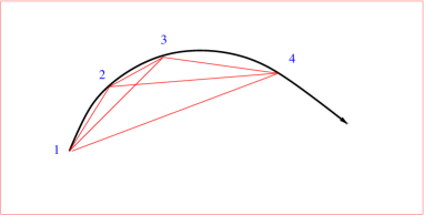
• Given three long, successive times $t_{1}<t_{2}<t_{3}$, and the corresponding correlations $C_{21},C_{32},C_{31}$, define for large times (see Fig. 3). $C_{31}=f(C_{21};C_{32})=\lim_{t_{1}\rightarrow\infty}f(C_{21};C_{32},t_{1})$, a ‘triangle relation’. Similarly for the integrated responses: $\chi(C_{31})=\tilde{f}[\chi(C_{21});\chi(C_{32})]$, i.e. the triangle relations $\tilde{f}$ and $f$ are isomorphic.

• Given any dynamic parameter $X_{AB}(t,t^{\prime})$ define for large times $X_{AB}(t,t^{\prime})\rightarrow X_{AB}\left[C_{AB}(t,t^{\prime})\right]$. We shall focus on cases in which this limit is non-trivial $X\neq 1$. This also implies that the integrated response becomes a function of the correlation: $\chi(t,t^{\prime})\rightarrow\chi(C(t,t^{\prime}))$.

• Given any two correlations of the system $\bar{C}(t,t^{\prime})$ and $C(t,t^{\prime})$ we write, again in the large-time limit, $\bar{C}\rightarrow g(C)$ for some $g$.

A way of putting this is as follows: a reparametrization-invariant quantity is a function in which times have been eliminated in favor of a correlation at those times: the particular one used acts as a ‘clock’ with respect to which all other quantities can be referred.

It is very natural to separate those quantities that are reparametrization-invariant from the reparametrizations themselves. A procedure for this may be implemented numerically: see Castillo et al. (2002, 2003); Chamon et al. (2004, 2002); Chamon and Cugliandolo (2007); Chamon et al. (2011).

Figure 3: The triangle relation $f(a,b)$ is associative: $C_{41}=f[C_{43},f(C_{32},C_{21})]=f[f(C_{43},C_{32}),C_{21}]$: the function $f$ is associative.

III.4 Time scales

The reparametrizations we consider are such that they leave the triangle function $C_{13}=f(C_{12},C_{23})$ invariant. The function $f$ allows us to define, in a natural way, time scales in a reparametrization-invariant way.

The function $f(a,b)$ may be easily seen to be associative (see Fig 3). It is possible to classify all associative functions, it turns out that the correlation has special ‘skeleton’ values, that for simplicity we write here as a discrete and growing series, $q_{1},...,q_{k}$ that divide the possible correlation in intervals $(q_{1},q_{2}),(q_{2},q_{3})...(q_{k-1},q_{k})$ with the property that if $C_{12}$ and $C_{23}$ belong to two different intervals then $f(C_{12},C_{23})=\min(C_{12},C_{23})$. If, on the contrary, $a$ and $b$ are in the same interval, another law applies. Each interval corresponds to a time scale, defined in a reparametrization-invariant way. The correspondence between Parisi and a dynamic, ‘multi-thermalization’ scheme (to be defined below) holds at the level of these ‘skeleton’ values. Let us see some examples of two, three and infinitely many scales where the set of skeleton values corresopndo to a continuous interval.

Two scales

This is the most usual case. An example is when the correlation $0<C\leq 1$ and there is a value $q$ such that for the interval $q\leq C\leq 1$ the correlation is much faster than for the interval $0\leq C<q$. We have, for example:

• For a stationary case $C(t-t^{\prime})=(1-q)\;\bar{A}(t-t^{\prime})+q\;\bar{B}\left(\frac{t-t^{\prime}}{H(\tau_{0})}\right)$, where $H$ is a growing function of $\tau_{0}$.

• For an aging case $t>t^{\prime}$:
  $C(t,t^{\prime})=(1-q)\;A(t-t^{\prime})+q\;B\left(\frac{L(t^{\prime})}{L(t)}\right)=(1-q)\;A(t-t^{\prime})+q\;B\left(e^{h(t)-h(t^{\prime})}\right)$

where $(A,B,\bar{A},\bar{B})$ are functions decreasing from one to zero as their argument goes from zero to infinity. The time reparametrization $h(t)=\ln L(t)$ brings the aging form into a time-translational invariant form.

Three scales

Again, the correlation $0<C\leq 1$ and there two values $q_{0}$ and $q_{1}$ such that for the interval $q_{1}\leq C\leq 1$ the correlation is much faster than for the interval $q_{0}\leq C<q_{1}$, itself much faster than $0\leq C<q_{0}$ We have, for example, for the stationary state:

• $C(t-t^{\prime})=(1-q_{1})\;\bar{A}(t-t^{\prime})+(q_{1}-q_{0})\;\bar{B}\left(\frac{t-t^{\prime}}{H(\tau_{0})}\right)+q_{0}\;\bar{\bar{B}}\left(\frac{t-t^{\prime}}{\bar{H}({\tau_{0}})}\right)$

where $\bar{\bar{B}}$ is also decreasing from one to zero as their argument goes from zero to infinity. The timescales are nested as $\tau_{0}\rightarrow\infty$: $\bar{H}(\tau_{0})\gg H(\tau_{0})\gg 1$.

The function $f$ is the function $\min$ for correlations in any two different scales.

A continuum of scales

An important case is when there is a dense set of values of correlation in which for all values of correlation

$$f(C_{21},C_{32})=\min[g(C_{21}),g(C_{32})]$$ (17)

holds. An example is:

$$C(t,t^{\prime})={\cal{C}}\left(\frac{\ln(t-t^{\prime}+t_{0})}{\ln\tau_{0}}\right)$$ (18)

where $t_{0}$ is a constant. This form satisfies (17) when $\tau_{0}\rightarrow\infty$ . Note how simple ultrametricity appears in dynamics. The Sherrington-Kirkpatrick model (stationarized by shear or by parameter evolution, see next subsection) follows this law with astonishing precision. Contucci et al. (2020).

III.5 Bringing a system to a stationary form

Shear and evolving disorder render a system stationary. It came as a surprise that for small drive the resulting stationary system is by no means close to an equilibrium one (as in usual systems with small currents) but rather a time-reparametrized version of the aging system.

For many technical purposes it is convenient then, at least in numerical computations, to stationarize’ the system. The shear strength or the speed of evolution of the disorder becomes then the control parameter, substituting the self-generated waiting time of the aging situation.

III.6 The Multithermalization scheme

Having defined timescales and effective temperatures, we are ready to state the multithermalization scheme. For all observables $A,B$ the long-time response and correlation functions define an effective temperature $A,B$ as $T_{AB}(t,t^{\prime})$ which we may write using a correlation as a ‘clock’ $T_{AB}(t,t^{\prime})\rightarrow T_{AB}(C_{AB})$.

$\bullet$ Timescales defined on the basis of the correlation of any pair of observables are the same.

$\bullet$ The effective temperatures are, within a timescale, the same for all pairs of observables.

IV Susceptibility Lego

In this section we discuss naive linear response theory (LRT), and show that both in statics and in dynamics, the non-ergodic order parameter, $x(q)$ and $X(q)$ can be viewed as the generating functions, respectively in equilibrium and in dynamics of a set of responses to random perturbation to the Hamiltonian. Let us add a to the Hamiltonian a perturbation of the form of a $p$-spin long range Hamiltonian

$$H\rightarrow H+\epsilon_{p}H_{p}$$ (19)

$$H_{p}=-\frac{1}{N^{(p-1)/2}}\sum_{i_{1},...,i_{p}}h_{i_{1},...,i_{p}}S_{i_{1}}...S_{i_{p}}$$ (20)

The perturbations $H_{p}$ are bulk self-averaging quantities, and we have seen that in equilibrium take values $I^{(p)}_{eq}=\mathbb{E}(\omega(H_{p})/N=\beta\epsilon_{p}(1-\int dq\;P_{\epsilon}(q)q^{p})$.

As usual in linear response theory we can consider the limit of small $\epsilon$, $\chi^{(p)}_{eq}=\lim_{\epsilon_{p}\to 0}I^{(p)}/\epsilon_{p}=T\lim_{\epsilon_{p}\to 0}\lim_{N\to\infty}\frac{1}{N}\frac{\partial^{2}}{\partial\epsilon_{p}^{2}}\log Z$. If this limit is regular, simple measures of the the energy absorbed by the perturbation inform us on the correlations in the unperturbed system.

Analogously, in dynamics, we can write for the finite time expected value of $H_{p}$

$$I^{(p)}(t) = \mathbb{E}\langle H_{p}(t)\rangle_{dyn}$$ (21)

$$= \epsilon_{p}\int_{0}^{t}ds\;R(t,s)pC(t,s)^{p-1}$$ (22)

and introducing $\beta X(q)=\lim_{t,s\rightarrow\infty\atop C(t,s)=q}\frac{R(t,s)}{\partial C(t,s)/\partial s}$ we have

$$\lim_{t\to\infty}I^{(p)}(t) = \beta\epsilon_{p}\int dq\;X(q)\;pq^{p-1}$$ (23)

As in the case of equilibrium $X$ is the generator function of response in presence of the perturbation and if its $\epsilon\to 0$ limit is regular, we have information about the response in the unperturbed system.

IV.1 Triangles

One can define higher order susceptibilities that in equilibrium allow one to reconstruct the probability distribution of several replicas, and in dynamics reflect the relations of correlations at different times. Particularly interesting are the ones associated to the probability of triangles $P(q_{12},q_{13},q_{23})$, which within Parisi RSB is concentrated on ultrametric triangles. In FMPP the triangle probabilities were reconstructed by considering average values of mixed combinations of the two different $H_{p}$, where the tensors defining the interactions are contracted over a subset of indexes, namely, in presence of the perturbations $H_{n+m}$ and $H_{n+l}$ in the Hamiltonian one considers the average value of the observable

$$O_{n;m,l}=\sum_{i_{1},...,i_{n+m+l}}J^{(n+m)}_{i_{1},...i_{n},j_{n+1},...,j_{n+m}}J^{(n+l)}_{i_{1},...i_{n},k_{n+1},...,k_{n+l}}S_{j_{n+1}}...S_{j_{n+m}}S_{k_{n+1}}...S_{k_{n+l}}.$$ (24)

where $n$ among the indexes of the two tensors, of rank $n+m$ and $n+l$ respectively, are contracted between them, and the others with the spins of the system.

Straightforward integration by part allows to see that in equilibrium

$$\frac{1}{N}\mathbb{E}\langle O_{n;m,l}\rangle=\beta^{2}\epsilon_{n+m}\epsilon_{n+l}\left(1-\langle q^{n+m}+q^{m+l}+q^{n+l}\rangle+2\langle q_{12}^{n}q_{13}^{m}q_{23}^{l}\rangle\right)$$ (25)

while in dynamics

$$\frac{1}{N}\mathbb{E}\langle\delta O_{n,m,l}(t)\rangle=\epsilon_{n+m}\epsilon_{n+l}\int_{0}^{t}dv\int_{0}^{t}du ([lC(t,v)^{l-1}R(t,v)][C(v,u)^{m}][nC(t,u)^{n-1}R(t,u)]+$$ (26)

$$[lC(t,v)^{l-1}R(t,v)][mC(v,u)^{m-1}R(v,u)][C(t,u)n]+$$

$$[C(t,v)l][mC(u,v)^{m-1}R(u,v)][nC(t,u)^{n-1}R(t,u)])$$

Since $\langle O_{n;m,l}\rangle$ is not directly a response function (i.e. a derivative of the free-energy) its equilibration was considered plausible, but the relation between triangles was not-completely proven within LRT. To remedy to this weakness, in Kurchan (2021) it was shown that in fact the triangular correlations could also be generated as responses to perturbations: it suffices to perturb the Hamiltonian with the following term

$$\delta H_{n,m,l}=(\gamma_{ml}O_{n;m,l}+\gamma_{nl}O_{m;n,l}+\gamma_{nm}O_{l;n,m})$$ (27)

that generates the triangles at the cubic order in the $\gamma$’s.

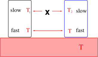
2. Overlap equivalence between sublattices

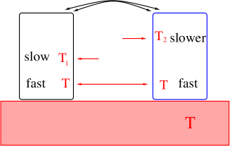
Another generating function that has proven useful is the following Let us first consider a lattice system, which we divide in four sublattices. whose components we shall call $s^{(1)}_{i}$, $s^{(2)}_{i}$ and $s^{(3)}_{i}$ and $s^{(4)}_{i}$. Adding to the energy a term

$$S = \frac{\gamma}{N}\sum_{ij}\left(h^{(1)}_{ij}h^{(2)}_{jk}s^{(1)}_{k}s^{(2)}_{i}+h^{(2)}_{ij}h^{(3)}_{jk}s^{(2)}_{i}s^{(3)}_{k}+h^{(3)}_{ij}{h}^{(4)}_{jk}s^{(3)}_{i}s^{(4)}_{k}\right)$$

with the $h^{(\ell)}_{ij}$ random Gaussian variables and computing the following correlation and its associated response:

$$C^{(4)}(t,t^{\prime})=\frac{1}{N^{2}}\sum h^{(1)}_{ij}h^{(4)}_{jk}\left\langle s^{(1)}_{i}(t)s^{(3)}_{k}(t^{\prime})\right\rangle_{\gamma}\qquad$$ (29)

This generating function may be generalized to any number of sublattices, and it is useful to show that there is overlap equivalence if and only if the timescales at different effective temperatures are widely separated.

V The nucleation argument

As we have stressed, in the large limit, even in presence of ageing, the values of extensive and local single time observables should tend to asymptotic values. In mean-field systems with long range interactions these may or may not coincide with the corresponding values in equilibrium. In systems with finite range interactions in finite dimensions, on the other hand, these values should coincide with their Boltzmann-Gibbs equilibrium values. The usual argument which is advanced is that in finite dimensions there are always local relaxation mechanisms allowing for equilibration. As a consequence, for the bulk free-energy, the infinite-time limit and the thermodynamic limits commute. The same should be generically true for its derivatives, such as internal energy and static responses. Notice that this argument tells that any possible broken ergodicity state should be only marginally stable, since the introduction of a small extensive random perturbation destabilizes the old equilibrium states to the advantage of new ones with a more favorable energetic balance between old and new energy.

This does not of course prevent the practical existence of systems such as structural glasses where the relaxation times at low temperature are so high that the energy density remains off-equilibrium on geological scales. Notwithstanding this, the limiting situation of aging close to equilibrium is a useful conceptualization to understand how glasses explore the configuration space. Whether in actual experimental systems on lab time scale one is close or not to this situation has to be decided case by case, depending on the system the preparation and the external parameters. We believe that this should be the case for example of spin glasses below, but close enough to the critical temperature. In these systems local equilibrium develops on growing scales $\xi(t)$ and the asymptotic situation may be observed if the growth of this scale is not too slow. We have seen that a possible way to measure $P(q)$ function consists in introducing long range random perturbations. If one admits that these perturbations indeed equilibrate (at the level $\epsilon$) in off equilibrium dynamics, then one could reconstruct the Parisi function from simple off-equilibrium measures of the response. Unfortunately, the nucleation argument does not hold in presence of long range interaction, and one could cast doubts that small long range perturbations would induce metastable states with free-energy density $O(\epsilon)$ higher than the equilibrium one. These could trap the off-equilibrium dynamics, thus spoiling the static dynamic equivalence. Thinking about what it could go wrong, this appears as a very remote possibility for small $\epsilon$. Within mean-field, with a long range unperturbed Hamiltonian, where inducing metastability is certainly easier that in finite D, we do not know any case where the introduction of a perturbation induces a difference of order $\epsilon$ between the value of the asymptotic dynamical energy and its equilibrium counterpart.

To obviate to this problem however, one can look for local perturbations giving rise to the same correlation functions within Linear Response. In FMPP it was suggested that this could be achieved diluting the $p$-spin perturbations so that they reduce to finite range interactions.

Let see how this works for $p=2$, the generalization to arbitrary $p$ being straightforward (and discussed in detail in FMPP). To fix the idea consider a spin system on a $D$ dimensional square lattice of size $L$, $\Lambda=\{1,...,L\}^{D}$. One can divide the lattice in two halves, $\Lambda_{l}$ and $\Lambda_{r}$, where the one of the coordinates, say in direction of the x-axes $e$, take the values $\{1,...,L/2\}$ and ${L+1,...,L}$ respectively. Let us add to the original Hamiltonian a perturbation of the form $\epsilon_{2}H_{2}$, with with

$$H_{2}=\sum_{x\in\Lambda_{-}}h_{x}S_{x}S_{T(x)}$$ (30)

where the $h_{x}$ are independent Gaussian random variables with unit variance, and $T(x)$ is a translation of $x$ of length $L/2$ in direction $e$. The thermal expectation value of the perturbation $H_{2}$ gives a contribution to the internal energy of the system which is extensive and self-averaging, i.e., independent (in the thermodynamical limit) of the particular realization of the disorder contained in either $H$ or $H_{2}$. The interaction $H_{2}$, which looks long range, is, in fact, a local perturbation in a different space. Let us rename the spins in the right-hand part so that if $x\in\Lambda_{l}$ then $T(x)\in\Lambda_{r}$ and $S_{T(x)}=S^{\prime}_{x}$. The total Hamiltonian can now be written as

$$H[S,S^{\prime}]=H_{l}[S]+H_{r}[S^{\prime}]+B[S,S^{\prime}]+\epsilon_{2}\sum_{x\in\Lambda_{-}}h_{x}S_{x}S^{\prime}_{x}$$ (31)

The Hamiltonian $H_{l}$ and $H_{r}$ refer, respectively, to the spins in $\Lambda_{l}$ and $\Lambda_{r}$. The term $B[S,S^{\prime}]$ is a surface term whose presence does not affect the average of $H_{2}$. Dropping it, the Hamiltonian (31) characterizes a spin system of size $L/2$ with two spins $S_{x}$ and $S_{x}^{\prime}$ on each site, and a purely local interaction. We have traded the long range interactions with a local coupling between among non-interacting or weakly coupled systems with different disorder and equal number of spins. We would like now to show that within LRT $H_{2}$ continues to be associated to the second moment of the overlap PDF. Simple integration by part in equilibrium reveals that

$$\langle H_{2}/N\rangle=\beta\epsilon_{2}\frac{1}{N}\sum_{x\in\Lambda_{l}}\left[1-\mathbb{E}\left(\langle S_{x}S_{T(x)}\rangle^{2}_{\epsilon}\right)\right].$$ (32)

In FMPP it was argued that the limit for $\epsilon\to 0$ of $\mathbb{E}\left(\langle S_{x}S_{T(x)}\rangle^{2}_{\epsilon}\right)$ both in presence or in absence of the boundary term $B[S,S^{\prime}]$ should be equal to the value that this correlation function takes for strictly zero coupling $\epsilon=0$ in presence of $B[S,S^{\prime}]$. The small coupling between the systems must have the same locking effect on the overlap as the surface interaction that we have discussed in the introduction.

V.1 Overlap equivalence if and only if timescale-separation

The property of overlap equivalence is very natural in the Parisi scheme. One has a distribution of states with their Gibbs weights. One now assumes that two pairs of states $(a,b),(c,d)$ having the same mutual overlap measured with one observable $q_{AA}(a,b)=q_{AA}(c,d)=q$, will have also the same mutual overlap measured with any other observable $q_{BB}(a,b)=q_{BB}(c,d)=\bar{q}$. This means that there is a universal function that gives, for every state, the second overlap if one knows the first:

$$\bar{q}=g(q)$$ (33)

Clearly, we have:

$$\bar{P}(\bar{q})d\bar{q}=P(g(q))dq\qquad\rightarrow\qquad\bar{P}(\bar{q})=P(g(q))\frac{1}{g^{\prime}(q)}$$ (34)

We may rewrite this putting $\frac{dx}{dq}=P(q)$ and $\frac{d\bar{x}}{d\bar{q}}=\bar{P}(\bar{q})$ as:

$$x(q)=\bar{x}(\bar{q})$$ (35)

The property (35) has the dynamic counterpart:

$$X(C)=\bar{X}(\bar{C})\qquad\rightarrow\qquad\bar{T}(\bar{C}(t,t^{\prime}))=T(C(t,t^{\prime}))$$ (36)

i.e. the effective temperature obtained from the fluctuation-dissipation relation of two observables at given times coincide.

This is very striking: a very similar relation arises from two apparently different arguments. And yet, using the second of the generating functions above, we find that there is a complete correspondence between $g,X,\bar{X}$ in the dynamic and in the equilibrium context.

In the dynamic case, we may also prove a strong result Kurchan (2021): overlap equivalence holds if and only if there is a wide separation of timescales associated to two different temperatures for each observable. The proof is not complicated: suppose we have two observables that have the same $X(C)=\bar{X}(\bar{C})$ at all times, but the times for different $X$’s are not really separate. Then, one can show that by coupling the observables one may construct a new correlation $\bar{\bar{C}}$ that does not have $\bar{\bar{X}}$ at the same times. In other words, Multithermalization is only consistent if the timescales of different temperatures are widely separated.

VI Commuting limits

We have seen that within naive perturbation theory, under the hypothesis of equilibration of bulk quantities, dynamics and equilibrium are in strong correspondence and the study of the dynamical response can be used to reconstruct the equilibrium Parisi function, which is an average over disorder realizations. This is at first sight strange, one has a relation between conceptually different kinds of objects that are relevant in different time regimes (in and out of equilibrium, respectively), when the system explores very different regions of phase-space.

In usual applications of LRT thermodynamic states are supposed to be stable against the introduction of a perturbation. For example if we introduce a small positive magnetic field $h$ in the low temperature Ising model we have

$$\langle S_{i}\rangle_{h}=\langle S_{i}\rangle_{+}+h\beta\sum_{j}(\langle S_{i}S_{j}\rangle_{+}-\langle S_{i}\rangle_{+}\langle S_{j}\rangle_{+})$$ (37)

Typical configurations of the perturbed systems are close to the unperturbed ones in the phase chosen by the field.

In disordered system by contrast, when a random perturbation is introduced this does not hold, the Gibbs state is marginally stable and ’chaotic’ Fisher and Huse (1986); Kondor (1989): the perturbation implies a complete reorganization of the Gibbs measure, which concentrates on regions with zero overlap with the unperturbed states

$$\frac{1}{N}\sum_{i=1}^{N}\mathbb{E}(\langle S_{i}\rangle\langle S_{i}\rangle_{0})=0.$$ (38)

Yet these regions should correspond to close values of the bulk quantities and similar statistical properties. The marginal stability of the Gibbs state should then correspond to the stochastic stability of the metastate and $P_{\epsilon}(q)\to P(q)$. In dynamics the situation is similar: the chaotic property imply that no matter how small a perturbation, a perturbed trajectory evolving with the same thermal noise as an unperturbed one, will stay close for a certain time, but will eventually diverge when time in large enough. Moreover, any random perturbation introduced after evolution up to a waiting time $t_{w}$ leads to a free-energy increase and hence to a rejuvenation of the system. This means that if we consider a field acting from $t_{w}$ to $t$, the limit for $h\to 0$ of the magnetization at time $t$, $\chi(t,t_{w})=\lim_{h\to 0}m(t,t_{w},h)/h$ is not uniform in time. As in the case of statics this does not prevent to use LRT. We just have to consider reparameterization invariant quantities (e.g. $\chi_{dyn}(q)=\int_{q}^{1}dq\;X_{\epsilon}(q)$), whose limit $\epsilon\to 0$ should be regular as the perturbation tends to zero.

VII The whole Parisi $\leftrightarrow$ multithermalization scheme needs time reparametrization invariance

All reparametrization-invariant relations between macroscopic quantities should coincide in dynamics and statics, where in statics only the ‘skeleton’ values are present. Ultrametricity, overlap equivalence and $x(q)$ are three examples. As we have mentioned above, the reciprocal is also true: if there is no timescale separation between different temperatures , there is no multithermalization, and no equilibrium overlap equivalence. There is however a problem. Consider two systems brought into weak contact from the beginning, for example two different lattice models, coupled locally so as to obtain a single model with two sublattices. Assume that at the same times the separate systems have non-coincident temperatures. This is perfectly possible, since the systems are independent. Now, couple weakly the two systems: should we conclude that the coupled system, for which there is no distinction between observables of one or the other system, violates the multithermalization scenario - and, a fortiori, the Parisi scheme? If this were so, both would be fragile to the point of irrelevance. The answer is surprising: the timescales of the systems rearrange so that different temperatures happen at different scales: thus, the combined system conforms to the scenario. But this needs to happen even for infinitesimal coupling, and it can only be possible if the system is ‘soft’ with respect to time-rearrangements of each temperature separately: in other words, it has to have independent time-reparametrization invariances in the slow dynamics limit. Such invariances, which we have already described above, where first reported by Sompolinsky and Zippelius Sompolinsky and Zippelius (1982, 1981) some forty years ago, and have recently had a crucial role in the interpretation of the SYK model Sachdev and Ye (1993) as a toy model of holography Kitaev (2015); Maldacena and Stanford (2016).

Figure 4: Caption

In conclusion, we realize that reparametrization softness is crucial for the consistency of the multi-thermalization scenario. But we have seen here that this scenario is in a one-to-one correspondence with the Parisi construction with replicas, at least in finite dimensions. We are thus led to ask ourselves, how do these reparametrizations appear in a replica treatment, where there is no time? To this we turn in the next section.

VIII Reparametrization invariance and replica space

VIII.1 A consequence of ultrametricity

In aging experiment the actual perturbation allowing to measure the function $X(q)$ is just an applied magnetic field. A small magnetic field $h$ acting from time $t_{w}$ to time $t$ induces a magnetization at time $t$ which is

$$m(t,t_{w})/h=\chi^{+}(t,t_{w})=\int_{t_{w}}^{t}ds\;R(t,s){\rightarrow\atop t,t_{w}\to\infty;C(t,t_{w})=q}\int_{q}^{1}dq^{\prime}X(q^{\prime}).$$ (39)

This suggests in equilibrium to consider the response to a magnetic field of a system $S_{1}$ which is kept to a fixed overlap $q\in{\mbox{Supp}}(P)$ with a configuration $S_{0}$ which is well equilibrated in absence of the perturbation.

Namely, considering an external random field term $\delta H=-\epsilon_{1}\sum_{i}h_{i}S_{i}$ with $\mathbb{E}h^{2}=1$ we would like to compute

$$\chi^{+}(q)=\frac{1}{\epsilon_{1}}\mathbb{E}\sum_{S_{0}}\frac{e^{-\beta H{[S_{0}]}}}{Z}\sum_{S}\frac{e^{-\beta(H{[S]}+\delta H[S])}\delta(Q(S,S_{0})-q)\sum_{i}h_{i}S_{i}}{Z_{1}[S_{0}]}$$ (40)

It is simple to see that within Linear Response Theory the response this is given by

$$\chi^{+}(q)=\beta\left(1-\mathbb{E}\;\left\langle\frac{\langle q_{12}\mathbbm{1}_{q_{10}=q_{20}=q}\rangle_{12}}{[\langle\mathbbm{1}_{q_{10}=q}\rangle]^{2}}\right\rangle_{0}\right)$$ (41)

where we have denoted as $\langle\cdot\rangle_{a,...}\cdot)$ the Boltzmann average with respect to the replicas $a,...$ Remarkably, using the Ghirlanda-Guerra identities, it is possible to show that this last quantity is equal to

$$\mathbb{E}\;\left\langle\frac{\langle q_{12}\mathbbm{1}_{q_{10}=q_{20}=q}\rangle_{12}}{[\langle\mathbbm{1}_{q_{10}=q}\rangle]^{2}}\right\rangle_{0}=\frac{\mathbb{E}\left({\langle q_{12}\mathbbm{1}_{q_{10}=q_{20}=q}\rangle_{012}}\right)}{\mathbb{E}\;\langle{[\langle\mathbbm{1}_{q_{10}=q}\rangle_{1}]^{2}}\rangle_{0}}=\int dq_{12}\;P(q_{12}|q_{10}=q_{20}=q)q_{12}$$ (42)

The conditional probability $P(q_{12}|q_{10}=q_{20}=q)$ is fixed by ultrametricity $P(q_{12}|q_{10}=q_{20}=q)=x(q)\delta(q_{12}-q)+\theta(q_{12}-q)P(q_{12})$. Which in turn implies that

$$\chi^{+}(q)=\beta\int_{q}^{1}dq\;x(q).$$ (43)

This has to be compared with the dynamical susceptibility at time $t$ to a field acting from time $t_{w}$ to $t$, in the long time limit having fixed $C(t,t_{w})=q$, namely

$$\chi_{dyn}^{+}(q)=\beta\int_{q}^{1}dq\;X(q).$$ (44)

The identity $X(q)=x(q)$ shows that the dynamical susceptibility tends to the constrained equilibrium susceptibility at large times. The result is simple and it has a clear interpretation. It means that asymptotically, during aging, given the configuration reached at a time $t_{w}$ partial equilibrium within the subspace with $C(t,t_{w})=q$ is essentially achieved before the system can relax to $q-\delta q$.

This deep property suggests that the reparametrization invariant part of the dynamics can be described through a fictive quasi-equilibrium process where the physical time is completely elimitated. The system is supposed to be in equilbrium on a correlation scale $q$ and to evolve to a scale $q^{-}$ choosing configurations according to the Gibbs distribution. Formally this correspond to the Markov chain defined by the following transition matrix

$$M_{q}({\bf S^{\prime}}|{\bf S})=\frac{1}{Z_{q^{-}}[{\bf S}]}\exp(-\beta H[{\bf S^{\prime}}])\delta(Q({\bf S^{\prime}},{\bf S})-q^{-})$$ (45)

where $Z_{q^{-}}[{\bf S}]$ is a restricted partition function normalizing the probability. The chain, that was called Boltzmann pseudo-dynamics in Franz and Parisi (2013); Franz et al. (2015) does not correspond to any physical dynamics, it implies macroscopic jumps from one configuration to the next one without solution of continuity. In Franz and Parisi (2013); Franz et al. (2015) however it was suggested that in a system with aging if one chooses $q=q_{EA}$ this fictitious dynamical process provides a coarse-grained reparamtrization invariant effective representation of the slow part of the relaxation below $q_{EA}$ of true dynamics: the system fully equilibrates in ’dynamical quasi-states’ Franz and Virasoro (2000) of amplitude $q_{EA}$ before relaxing below this value; in this relaxation the system explores the configuration space choosing new quasi-states at random with Boltzmann probability among the available ones, i.e. those lying at overlap $q_{EA}$. It is clear from the considerations of the previous section that thanks to Ultrametricity we can go further with the effective description and instead of coarse graining only the short times corresponding to $q_{EA}$, we could choose any arbitrary skeleton value of $q\in Supp(P)$, and the corresponding pseudo-dynamics (45) would just provide a reparametrization invariant representation of the relaxation below $q$ with the same physical content as the true dynamics.

IX Two, perhaps three finite-dimensional puzzles

IX.1 Is one-step RSB unstable in finite dimensions?

As we argued above, a system in finite dimensions must be reparametrization-soft and marginally stable, otherwise two systems with similar timescales and different effective temperatures would be unable to become a two-step RSB when weakly coupled. Analogously, a 1RSB system coupled with a fullRSB one must develop a continuum of effective temperatures and hierarchical time scales to become fullRSB itself.

In the mean-field case, however, the equilibrium of a one-step systems is not marginal. The situation is analogous to the ferromagnetic case, which is not marginal within mean-field (there is an extensive barrier between minima), while it becomes so in finite dimensions, being unstable with respect to a small uniform field  A hypothetical dynamical 1RSB state in finite dimension should be at least marginally stable against continuous RSB, a situation that could be called weak fullRSB. Such a situation would seem rather unnatural in a disordered system, by its nature heterogeneous, where the effective temperature would have spatial fluctuations. It is thus natural to conjecture that close to equilibrium, one-step, or more generally discontinuous solutions are unstable against higher RSB, thus leading to a situation where all the values of the correlations except the ones corresponding to the trivial equilibrium regime are ’skeleton’ values and full ultrametricity holds.

IX.2 Dynamic timescales in three and four dimensions

The experimental evidence of spin-glasses seems to point to only two timescales Berthier et al. (2000b); Vincent et al. (1997), and a non-trivial $P(q)$ Hérisson and Ocio (2002) with what appears to be many temperatures – i.e. the $\chi$ vs $C$ plot appears to have a curved section, apparently violating the Multithermalization. This however should be taken with a grain of salt as it could be preasymptotic effect. Perhaps a clarifying step would be to see whether the correlation decay in times of hours and days is fitted with the same time-dependence of the one in microseconds, a comparison that has not, to our knowledge, been done. The numerical evidence in three dimensions seems to point to overlap equivalence between site and link overlap Contucci et al. (2006), although we know that this is not possible if there is only one slow timescale and many temperatures. The probable explanation is that the violation is, however, too small to be observed numerically.

In four dimensions the situation is much more clear: the little evidence we have Stariolo (2001) seems to point resolutely to dynamic ultrametricity with many scales, just as in the Sherrington-Kirkpatrick model.

IX.3 Aging strongly far from equilibrium

Structural glasses as we know them in the laboratory find themselves in extremely long lived metastable states. The internal energy density, specific volume etc. persist to off-equilibrium values high above the equilibrium ones for at least geological times. Yet these systems slowly age. The response during physical aging in such conditions verifies to an excellent approximation scaling laws with a single effective time scale Struik (1977). Numerical simulations of model glasses indicate that a description in terms of a single effective temperature, reminiscent of Mean-field 1RSB systems is appropriate Parisi (1997); Barrat and Kob (1999). One can ask

One can conjecture that in such conditions, which are formally very far from the asymptotic situation needed to have quasi-equilibrium sampling and reparametrization invariance, the dynamics in the aging regime can still be approximately described in term of these concepts, as a quasi-equilibrium process where degrees of freedom that evolve on the same scales are in mutual ‘multithermalized’ equilibrium, and that a quasi-equilibrium process as in Franz and Parisi (2013); Franz et al. (2015) with an properly chosen $q$ would still be an appropriate quasi-reparameterization invariant description of the slow dynamics.

X Conclusions

We have discussed the deep connection between dynamic and equilibrium theoretical constructions as it is realized whenever during slow dynamics bulk expectation values are close to equilibrium, as it should asymptotically be the case in finite dimensional systems. In that case Linear Response Theory allows one to relate dynamical response functions to equilibrium correlations. Linear Response in disordered systems is, however, subtle.

The main elements at play are the softness displayed by these systems both in equilibrium and off-equilibrium with respect to random perturbations, and somewhat paradoxically, the stability of appropriately defined responses and correlations with respect to the same perturbations.

It seems fair to say that the evolution of the subject has been from an almost miraculous ansatz to the gradual understanding of the questions it raises on more robust and method-independent properties.

Acknowledgments We acknowledge the support of the Simons Foundation, Grants No 454941 S. Franz No 454943 J. Kurchan.

References

- Mézard et al. (1987) M. Mézard, G. Parisi, and M. A. Virasoro, Spin Glass Theory and Beyond (World Scientific, Singapore, 1987).
- Thalmann (2001) F. Thalmann, The European Physical Journal B-Condensed Matter and Complex Systems 19, 65 (2001).
- Berthier et al. (2000a) L. Berthier, J.-L. Barrat, and J. Kurchan, Physical Review E 61, 5464 (2000a).
- Horner (1992) H. Horner, Zeitschrift für Physik B Condensed Matter 86, 291 (1992).
- Sompolinsky and Zippelius (1982) H. Sompolinsky and A. Zippelius, Physical Review B 25, 6860 (1982).
- Sompolinsky and Zippelius (1981) H. Sompolinsky and A. Zippelius, Physical Review Letters 47, 359 (1981).
- Cugliandolo and Kurchan (1993) L. F. Cugliandolo and J. Kurchan, Phys. Rev. Lett. 71, 173 (1993).
- Cugliandolo and Kurchan (1994) L. F. Cugliandolo and J. Kurchan, Journal of Physics A: Mathematical and General 27, 5749 (1994).
- Franz and Mézard (1994) S. Franz and M. Mézard, EPL (Europhysics Letters) 26, 209 (1994).
- Cugliandolo et al. (1997) L. F. Cugliandolo, J. Kurchan, and L. Peliti, Phys. Rev. E 55, 3898 (1997).
- Contucci et al. (2019) P. Contucci, J. Kurchan, and E. Mingione, Journal of Physics A: Mathematical and Theoretical 52, 324001 (2019).
- Contucci et al. (2020) P. Contucci, F. Corberi, J. Kurchan, and E. Mingione, arXiv preprint arXiv:2012.03922 (2020).
- Franz et al. (1998) S. Franz, M. Mézard, G. Parisi, and L. Peliti, Physical Review Letters 81, 1758 (1998).
- Franz et al. (1999) S. Franz, M. Mezard, G. Parisi, and L. Peliti, Journal of statistical physics 97, 459 (1999).
- Kurchan (2021) J. Kurchan, arXiv preprint arXiv:2101.12702 (2021).
- Sherrington and Kirkpatrick (1975) D. Sherrington and S. Kirkpatrick, Physical review letters 35, 1792 (1975).
- Parisi (1979) G. Parisi, Physical Review Letters 43, 1754 (1979).
- Talagrand et al. (2003) M. Talagrand et al., Spin glasses: a challenge for mathematicians: cavity and mean field models, Vol. 46 (Springer Science & Business Media, 2003).
- Panchenko (2013a) D. Panchenko, The sherrington-kirkpatrick model (Springer Science & Business Media, 2013).
- Fisher and Huse (1986) D. S. Fisher and D. A. Huse, Physical review letters 56, 1601 (1986).
- Bray and Moore (1987) A. J. Bray and M. A. Moore, Physical review letters 58, 57 (1987).
- Franz and Toninelli (2004) S. Franz and F. L. Toninelli, Journal of Physics A: Mathematical and General 37, 7433 (2004).
- Ghirlanda and Guerra (1998) S. Ghirlanda and F. Guerra, Journal of Physics A: Mathematical and General 31, 9149 (1998).
- Panchenko (2013b) D. Panchenko, Annals of Mathematics , 383 (2013b).
- Aizenman and Contucci (1998) M. Aizenman and P. Contucci, Journal of statistical physics 92, 765 (1998).
- Arous and Guionnet (1995) G. B. Arous and A. Guionnet, Probability Theory and Related Fields 102, 455 (1995).
- Ben Arous et al. (2006) G. Ben Arous, A. Dembo, and A. Guionnet, Probability theory and related fields 136, 619 (2006).
- Barrat and Kob (1999) J.-L. Barrat and W. Kob, EPL (Europhysics Letters) 46, 637 (1999).
- Berthier et al. (1999) L. Berthier, J.-L. Barrat, and J. Kurchan, The European Physical Journal B-Condensed Matter and Complex Systems 11, 635 (1999).
- Parisi (1983) G. Parisi, Physical Review Letters 50, 1946 (1983).
- Franz et al. (1992) S. Franz, G. Parisi, and M. Virasoro, EPL (Europhysics Letters) 17, 5 (1992).
- Parisi and Talagrand (2004) G. Parisi and M. Talagrand, Comptes Rendus Mathematique 339, 303 (2004).
- Franz and Parisi (1995) S. Franz and G. Parisi, Journal de Physique I 5, 1401 (1995).
- Franz and Parisi (1998) S. Franz and G. Parisi, Physica A: Statistical Mechanics and its Applications 261, 317 (1998).
- Temesvári et al. (2000) T. Temesvári, I. Kondor, and C. De Dominicis, The European Physical Journal B-Condensed Matter and Complex Systems 18, 493 (2000).
- De Dominicis and Giardina (2006) C. De Dominicis and I. Giardina, Random fields and spin glasses: a field theory approach (Cambridge University Press, 2006).
- Castellani and Cavagna (2005) T. Castellani and A. Cavagna, J. Stat. Mech. 2005, P05012 (2005).
- Castillo et al. (2002) H. E. Castillo, C. Chamon, L. F. Cugliandolo, and M. P. Kennett, Phys. Rev. Lett. 88, 237201 (2002).
- Castillo et al. (2003) H. E. Castillo, C. Chamon, L. F. Cugliandolo, J. L. Iguain, and M. P. Kennett, Phys. Rev. B 68, 134442 (2003).
- Chamon et al. (2004) C. Chamon, P. Charbonneau, L. F. Cugliandolo, D. R. Reichman, and M. Sellitto, J. Chem. Phys. 121, 10120 (2004).
- Chamon et al. (2002) C. Chamon, M. P. Kennett, H. E. Castillo, and L. F. Cugliandolo, Phys. Rev. Lett. 89, 217201 (2002).
- Chamon and Cugliandolo (2007) C. Chamon and L. F. Cugliandolo, J. Stat. Mech. 2007, P07022 (2007).
- Chamon et al. (2011) C. Chamon, F. Corberi, and L. F. Cugliandolo, J. Stat. Mech. 2011, P08015 (2011).
- Kondor (1989) I. Kondor, Journal of Physics A: Mathematical and General 22, L163 (1989).
- Sachdev and Ye (1993) S. Sachdev and J. Ye, Phys. Rev. Lett. 70, 3339 (1993).
- Kitaev (2015) A. Kitaev, “A simple model of quantum holography,” (2015), A simple model of quantum holography, http://online.kitp.ucsb.edu/online/entangled15/kitaev/, http://online.kitp.ucsb.edu/online/entangled15/kitaev2/.
- Maldacena and Stanford (2016) J. Maldacena and D. Stanford, Phys. Rev. D 94, 106002 (2016).
- Franz and Parisi (2013) S. Franz and G. Parisi, Journal of Statistical Mechanics: Theory and Experiment 2013, P02003 (2013).
- Franz et al. (2015) S. Franz, G. Parisi, F. Ricci-Tersenghi, and P. Urbani, Journal of Statistical Mechanics: Theory and Experiment 2015, P10010 (2015).
- Franz and Virasoro (2000) S. Franz and M. A. Virasoro, Journal of Physics A: Mathematical and General 33, 891 (2000).
- Berthier et al. (2000b) L. Berthier, J.-L. Barrat, and J. Kurchan, Physical Review E 63, 016105 (2000b).
- Vincent et al. (1997) E. Vincent, J. Hammann, M. Ocio, J.-P. Bouchaud, and L. F. Cugliandolo, in Complex Behaviour of Glassy Systems (Springer, 1997) pp. 184–219.
- Hérisson and Ocio (2002) D. Hérisson and M. Ocio, Physical Review Letters 88, 257202 (2002).
- Contucci et al. (2006) P. Contucci, C. Giardina, C. Giberti, and C. Vernia, Physical review letters 96, 217204 (2006).
- Stariolo (2001) D. A. Stariolo, EPL (Europhysics Letters) 55, 726 (2001).
- Struik (1977) L. C. E. Struik, (1977).
- Parisi (1997) G. Parisi, Physical review letters 79, 3660 (1997).