A machine-learning-based tool for last closed-flux surface reconstruction on tokamaks

Abstract

Nuclear fusion represents one of the best alternatives for a sustainable source of clean energy. Tokamaks allow to confine fusion plasma with magnetic fields and one of the main challenges in the control of the magnetic configuration is the prediction/reconstruction of the Last Closed-Flux Surface (LCFS). The evolution in time of the LCFS is determined by the interaction of the actuator coils and the internal tokamak plasma. This task requires real-time capable tools able to deal with high-dimensional data as well as with high resolution in time, where the interaction between a wide range of input actuator coils with internal plasma state responses add additional layer of complexity. In this work, we present the application of a novel state of the art machine learning model to the LCFS reconstruction in the Experimental Advanced Superconducting Tokamak (EAST) that learns automatically from the experimental data of EAST. This architecture allows not only offline simulation and testing of a particular control strategy, but can also be embedded in the real-time control system for online magnetic equilibrium reconstruction and prediction. In the real-time modeling test, our approach achieves very high accuracies, with over 99% average similarity in LCFS reconstruction of the entire discharge process.

Keywords: time series, magnetic reconstruction, tokamak

1 Introduction

Thermonuclear fusion power is one of the ideal forms of clean and sustainable energy that has the potential to meet our future energy needs, while being inherently safe and potentially a limitless source of energy. A tokamak is a leading magnetic confinement fusion device for generating controlled thermonuclear fusion power. One core research of tokamak physics is the control of the magnetic fields distribution which is needed to keep the plasma confined. Magnetic control is not trivial, in particular for advanced configurations, since the resulting distribution of the magnetic fields is determined by the interaction of complex, sometimes unpredictable plasma state evolution and a wide range of actuator inputs. Therefore, tools capable of reconstructing efficiently and reliably the evolution of magnetic fields [1, 2, 3, 4] are of paramount importance both for the design of experiments as well as for developing robust control strategies. The conventional approach to this time-varying, non-linear, high-dimensional task is to solve an inverse problem to pre-compute a set of actuator coil (poloidal field coils etc) currents and voltages [5, 6, 3]. Then, the real-time estimate of the tokamak plasma equilibrium through a simulation code [7, 4, 8] allows modulating actuators coil voltages to achieve the desired target. Although these physical simulation codes are usually effective, they require substantial effort and expertise by physicists to adapt a model whenever the tokamak magnetic configuration is changed. To overcome these bottlenecks, fusion community has recently started investigating machine learning (ML) and artificial intelligence (AI) capabilities to reduce the complexity of models and numerical codes.

Full tokamak discharge modeling is a critical task also from a computational point of view. The typical workflow required for tokamak modeling, known as "Integrated Modeling" [9], is computationally very expensive. For instance, a few seconds’ discharge process generally takes hours to days of computation for high fidelity simulations. Moreover, the integration of the many physics processes required to describe the evolution of the plasma state adds an even further layer of complexity. In this context, a common approach is to replace high fidelity simulation codes with ML-based surrogate models. This allows to accomplish the same task significantly reducing computation time while preserving a reasonable level of accuracy.

Recently, various applications in magnetic confinement fusion research have relied on machine learning approaches to solve a variety of problems, including disruption prediction [10, 11, 12, 13, 14, 15, 16], electron temperature profile estimation [17], surrogate model [18, 19, 20], plasma tomography [21], radiated power estimation [22], discharge estimation [23, 24], identifying instabilities [25], neutral beam effects estimation [26], classifying confinement regimes [27], determination of scaling laws [28, 29], filament detection [30], coil current prediction with the heat load pattern [31], equilibrium reconstruction [17, 32, 33, 34, 35, 36], and equilibrium solver [37], control plasma [38, 39, 40, 41, 42, 43], physic-informed machine learning [44], reinforcement learning-informed magnetic field control [3]. In particular, the use of reinforcement learning for magnetic field control work has a different target from our work, which is the design of a controller for magnetic control during the flat-top of the plasma current. The conventional controller should take it over in the ramp-up and ramp-down phases.

Modeling the entire tokamak discharge process by leveraging machine learning approaches is challenging both from a technical and computational point of view. The duration of a plasma discharge in EAST [45] can be of the order of thousands of seconds, with a resulting sequence length that exceeds $1\text{$\times$}10^{6}$ if the sampling rate is $1kHz$. There are different classes of machine learning models to deal with sequence problems, RNNs [46] Transformers [47] based on the attention mechanism, and several variants. For the traditional RNN algorithm, training and inference time on the long sequence are usually slow. The sequential nature of RNN models prevents in general achieving a high level of parallelization in computations. From a machine learning perspective, the processing of long time sequences characterized by short and long terms dependencies is still an outstanding challenge. In the plethora of deep learning models, transformers are a novel architecture which allows overcoming some of the aforementioned issues thanks to the multi-head-attention mechanism. Nevertheless, also the use of transformers for modeling long sequences presents some limitations due to their computational complexity $O(n^{2}d)$, where $n$ is the sequence length. In practice, when the sequence length is of the order of thousands of samples and we are dealing with high-dimensional data, training and inference times start to become unacceptable for most of the applications.

The magnetic field reconstruction has two research paradigms: physics-driven and data-driven approaches. Physics-driven approaches in magnetic field reconstruction have been studied for the last decades, resulting in the development of various simulation codes, such as Equilibrium Fitting (EFIT)[48, 49, 50], LIUQE [51], RAPTOR [52]. The adaptation of these codes to new target plasma configurations or to new machines requires a non-negligible effort. This aspect, together with the aspect of computational efficiency, has recently brought the fusion community to leverage more and more data-driven methods to solve tasks at different levels of complexity. However, magnetic reconstruction is far behind other applications in fusion. To the best of our knowledge, only a few works such as [3], have actually been deployed and successfully tested in a real environment.

In this paper, two different variants of 1D Shifted Windows Transformer model (1D-SWIN Transformer) have been proposed for, respectively, real-time and offline magnetic reconstruction of the LCFS. In the case of the 1D-SWIN Transformer, model computational complexity depends linearly on the sequence length n. Moreover, these models can take advantage of a high level of parallelization thanks to the attention mechanism and the non-sequential nature of the algorithm. The models presented in this work are trained only on experimental data and can be used for the estimation of the magnetic field evolution for the entire length of the tokamak discharge, including the ramp-up and the ramp-down phases of the plasma current.

As far as the real-time estimation of the magnetic fields evolution is concerned, the model is not directly used to control the magnetic field. It is able to predict the evolution of the magnetic field one step ahead in the future, allowing to design more effective feedback control strategies. The real-time model can be integrated within the plasma control system (PCS) to assist robust magnetic control by predicting the magnetic field in the subsequent time step. The offline model reduces remarkably the execution time required to simulate the evolution of the magnetic field for the entire discharge. Moreover, when coupled to other ML-based surrogate models for the prediction of 0D quantities like in [23], it allows to simulate the evolution of various quantities of interest, supporting the experimental design as well as the optimization of the target plasmas. Compared to the model described in [3], our model does not rely on a physics simulation code, whose computational complexity cannot be ignored. Additionally, given the regression task, the training of our model is in general more efficient than the training of a model based on reinforcement learning. Another non-negligible aspect, which is of increasing importance in fusion as well as in many other fields of science, is that transformers have become particularly successful when used in the context of transfer learning. The key concept is that the model has the capability to learn the underlying dynamics characterizing the evolution of the magnetic field in a tokamak, encoding this knowledge in a reduced latent space representation that can be “easily” adapted to new devices. Such a perspective is extremely attractive and would allow to significantly optimize the exploitation of fusion devices for more and more advanced studies.

According to the main quantities required for magnetic field control [2], the data used to build the machine learning model are mainly magnetic signals and references for control, namely magnetic surface probes data, in-vessel currents, poloidal field coils data, flux loop data, plasma current and shape references. For the real-time version of the model, the average similarity is over 99%, and the inference time is 0.7 ms (<1 ms in accordance with the typical control system requirements). For the offline version of the model, the average similarity is over 93%, and the average inference time is ~0.22 s for sequence length $1\times 10^{6}$, which is lower than the real-time model because of different settings, as it will be discussed in the following sections.

Our contributions are summarized as follows:

1. We propose a generalized 1D shifted windows transformer architecture that can compute long time series.

2. One of the models can be integrated into tokamak control for estimating in real-time magnetic field in advance.

3. One of the models can also be combined with a 0D proposal estimation model to give a complete prediction for experimental proposal results.

4. The validity of the proposed models is demonstrated over a large experimental data set of the EAST tokamak.

2 Results

We trained, validated, and tested real-time and offline versions of the proposed transformer-based model on the dataset during the 2016-2020 EAST campaigns with shots number in the range #52804-88283 [53, 54, 55], whereas input and output signals can be found in section 4.2. The similarity metric used to test the model is defined as follows:

$$S\left(\boldsymbol{x},\boldsymbol{y}\right)=\max\left(\frac{\Sigma(\boldsymbol{x}-\bar{\boldsymbol{x}})(\boldsymbol{y}-\bar{\boldsymbol{y}})}{\sqrt{\Sigma(\boldsymbol{x}-\bar{\boldsymbol{x}})^{2}\Sigma(\boldsymbol{y}-\bar{\boldsymbol{y}})^{2}}},0\right),$$ (1)

2.1 Offline model results

Figure 1 shows our offline model prediction for the Last Closed-Flux Surface (LCFS) in the EAST shot #73678. The duration of this shot is longer than 70s, with a the sequence length of $\sim 7\text{$\times 10^{4}$}$, which is a typical long sequence modeling problem. The LCFS shown in the figure is generated through the equilibrium reconstruction code EFIT [50] by inputting the magnetic quantities predicted by the model into EFIT. The equilibrium reconstruction is a broad topic in tokamak research, extensively discussed in various papers and main plasma physics books [56], and therefore it will not be addressed in this paper. Figure 1 shows the model has reconstructed with high accuracy the LCFS not only during the flat-top phase of the plasma current, but also in the ramp-up and ramp-down phases, which are non-stationary phases. The model is able to reproduce the magnetic configuration during the various discharge phases, from the tokamak start-up “cycle”, going through the formation of the “single null” shape, to the characteristic shapes in the shut-down “cycle”.

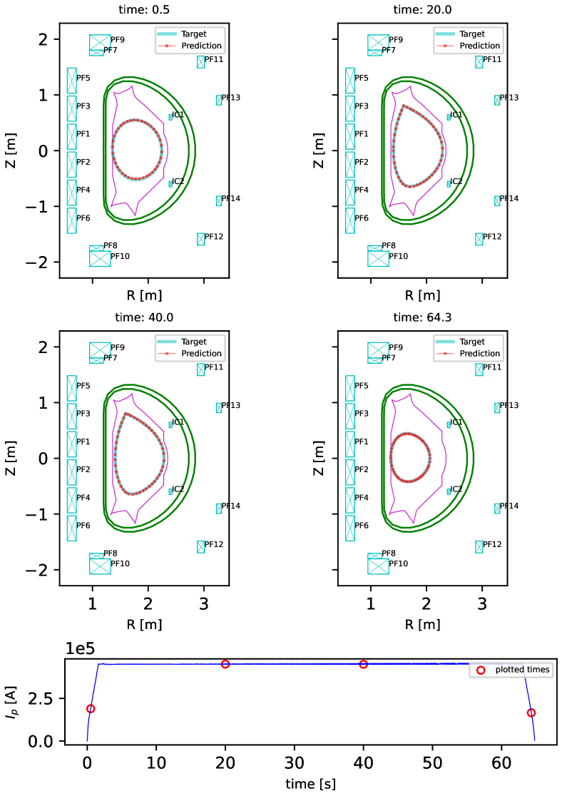
Figure 1: Shot #73678 offline magnetic reconstruction. The LCFS was generated from EFIT using inputs from our model. The solid blue lines are the experimental target LCFS, the red “star” markers are predicted LCFS.

The performance of the model has been evaluated with the same similarity indicator discussed in [23]. The average similarity in the test set for the offline version of the model, as shown in figure 2, is 93.2%. Most of the shots are concentrated around 95%, with the bulk of the distribution above 90%. The test set for this work consists of experiments in the shot range #82651-88283 for a total of 1677 shots, some of which with a very long duration (see details in section 4.2). Note that the similarity is computed on raw signal data instead of the reconstructed LCFS. As far as experiments with similarity less than 0.85 are concerned, there are 98 shots, among which, 89 are disruptions, whereas 9 are shots with a regular termination. A disruption is an unexpected termination of the discharge where the plasma loses abruptly its thermal and magnetic confinement, involving huge electromagnetic forces and thermal loads, which can potentially damage the machine. Apart from experiments dedicated to the study of disruption physics and to the assessment of engineering limits during these violent transients, the design of the discharge itself together with robust real-time control strategies aim to avoid disruptions. Nevertheless, when operating close to stability limits, various sequence of events can potentially lead to disruption, strongly affecting the magnetic equilibrium and making it unavoidably deviate from offline modeling. The operational space characterizing disruptions is extremely complex and wide, making its coverage within the input domain unfeasible. The 9 regular terminations with relatively high error are not well estimated probably because of inherent limitations in the model, or inaccuracies in the measurements, but they correspond to only the 0.5% of the test set.

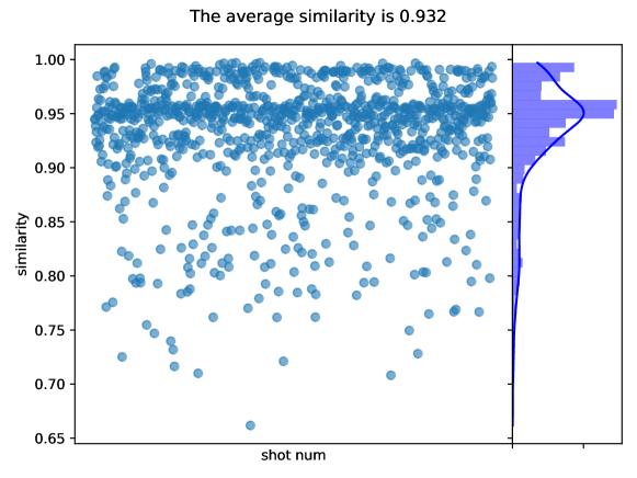
Figure 2: Similarity distribution of offline model predicted results on the test set. The test set (see section 4.2) is in shot range #82651-88283 and some long-time shots for a total of 1677 shots.

2.2 Real-time model results

The real-time model differs from the offline model both in terms of input quantities and inference time requirements (discussed in detail in section 4.1). Figure 3 shows the reconstruction results of the real-time model for the shot #73678. In real-time settings, the real measurement of the magnetic field probe at the previous step is fed as input to simulate the actual tokamak control feedback process.

Figure 3: Shot #73678 real-time magnetic reconstruction. The LCFS was generated by the same method as with offline magnetic reconstruction, figure 1. The solid blue lines are the target LCFS, the red “star” markers are predicted LCFS.

The similarity of the real-time model in the test set is shown in figure 4, which is the same test set as the offline model.

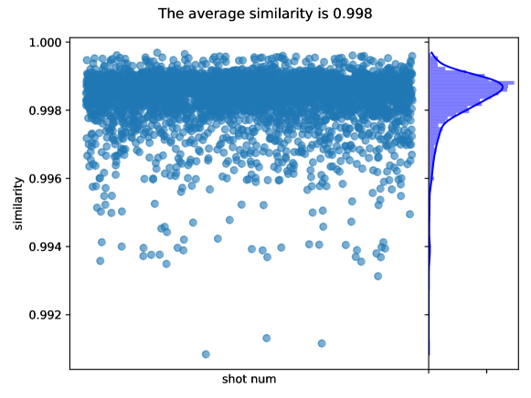
Figure 4: Similarity distribution of real-time model predicted results on the test set. The test set for the real-time and the offline models are the same.

Although there is almost no difference between the modeling results of shot 73678 in figure 1 and figure 3, comparing figure 2 and figure 4, it can be found that the real-time model performs slightly better than the offline model. A possible reason is that the plasma magnetic field is not a rapidly time-varying process, and the system output at the current time step is a good “guide” to forecast the evolution of the system in the subsequent time step. However, the offline model has no knowledge of the actual tokamak output, so even if bigger and more computationally demanding models are used for the offline task, the results are a bit less accurate compared to the real-time model.

3 Discussion

In the current work, we propose a 1D shifted windows transformer model that can work with long sequences (up to $1\times 10^{6}$ sequence length for LCFS reconstruction in this work), which reduces the computational complexity of the original model from a square to a linear dependence to the sequence length. The proposed model can form a general sequence processing backbone network for both real-time and offline sequence modeling. Thanks to the reduced computational complexity, the model can be efficiently used for very long sequences, exceeding $1\times 10^{6}$ sequence length, as we demonstrate in this study. To the best of our knowledge, we have achieved the first data-driven modeling of the LCFS for the whole tokamak discharge, including the ramp-up and the ramp-down phases of the plasma current. Being dynamic phases, ramp-up and ramp-down are in general more difficult to model, and as such they are often not taken into account in data-driven applications. The inference time for the real-time task (one-step ahead forecasting) is $\sim 0.7ms$ with an average similarity of >99%, while the average inference time for the offline modeling (entire discharge process) is 0.22s with an average similarity of >93%.

From the machine learning point of view, to the best of our knowledge, this work is also the first proposing an attention-based mechanism for successfully modeling long time sequences. From the point of view of tokamak physics research, we have achieved high accuracy and fast tokamak magnetic field modeling, which can be used for critical applications such as real-time control or offline validation of tokamak’s experimental proposals. If integrated with other existing discharge modeling data-driven frameworks, such as [23], the proposed approach can represent an extremely valuable tool to advance in the development of robust and high-performance tokamak scenario. A first important milestone for the future will be the actual integration of the real-time model within the plasma control system, which is of paramount importance to understand how reliable these systems are when operating routinely in a real environment. Another exciting future perspective triggered by the achievements documented in this work is the validation of the full modeling of the plasma discharge, integrating magnetic reconstruction with the prediction of key 0-D physics quantities commonly describing the outcome of a plasma discharge. Finally, extending and testing the 1D shifted windows transformer to other general areas of machine learning such as NLP is also an exciting direction for future research.

4 Methods

4.1 Machine learning Model

The general architecture of our machine learning models is shown in figure 5. Our architecture uses a customized 1D shifting window attention mechanism inspired by the Swin transformer [57] to model long-term dependencies and interactions between inputs and outputs. We stack self-attention blocks to build the machine learning model.

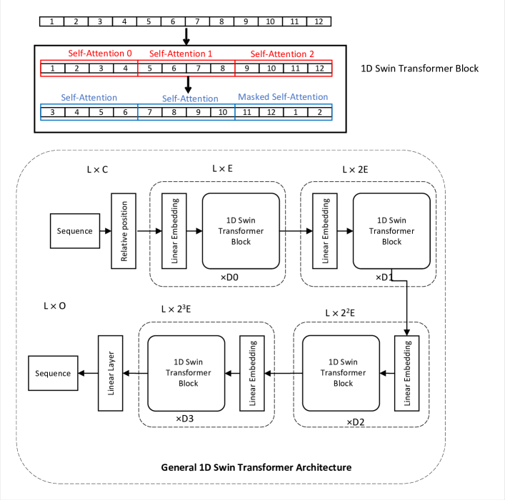
Figure 5: Our machine learning model architecture. In the figure, “L” is sequence length, “E” is the embedded dimension, “C” is the input sequence channels number, and “O” is the output sequence channels number.

In the framework of deep-learning, there are four main candidate architectures for modeling such long-time sequences: convolutional neural network (CNN), recurrent neural network (RNN) such as long-short term memory (LSTM) and gated recurrent unit (GRU), Transformer, and our customized 1D SWIN transformer. In addition, some critical quantitative criteria should be taken into account for modeling tokamak magnetic probe data: computational complexity, number of sequential operations, and maximum path length[58]. From table 1, 1D shifting window attention has roughly as many sequential operation and computational complexity as CNNs. Generally, the attention mechanism can achieve superior performance with respect to CNN in numerous time sequence tasks, such as natural language processing [47, 59].

Table 1: CNN, RNN, Transformer, 1D SWIN transformer comparison.

Model Type	Computational complexity	Sequential operation	Maximum path length
CNN	$O(knd^{2})$	$O(1)$	$O(n/k)$
RNN	$O(nd^{2})$	$O(n)$	$O(n)$
Transformer	$O(n^{2}d)$	$O(1)$	$O(1)$
1D SWIN transformer	$O(w^{2}nd)$	$O(1)$	$O(n/w)$

Where $k$ is kernel size of CNN, $d$ is sequence dimension, $n$ is sequence length, $w$ is window size of 1D SWIN transformer

Generally speaking, there should be some differences between the real-time and offline model-building strategies. The real-time model requires that the single-step inference is fast enough. That is, the one-step inference time of the model should be less than the response time required by the control system, and the actual system output of the previous step can be fed back as input to the model. According to the requirements of the EAST magnetic control system, model inference time should be less than 1 ms. For a typical transformer model, single-step input is complex. If the preset control commands are modified, the whole sequence needs to be recalculated, which makes the inference time exceed the control system requirements. In our work, we let “window size” = 1, which makes our model calculate the attention only in the channel axis, and single-step input becomes less expensive. This design of the model results in a one-step inference time of $\sim 0.7ms$, which allows satisfying real-time constraints. For the offline model, the actual system output from the previous step should not be fed back as input unless it is trained using the teaching force trick. The time requirement of the offline mode can be relaxed, but it should generally be within one hour. Otherwise, the advantage of the machine learning model over the integrated modeling model will be diminished. If we use the teaching force, we have to recompute all the past sequences step-by-step, so the inference time of the entire sequence will be in the order of $1\times 10^{5}s$ for the reason of the computational complexity. This paper’s offline model does not use the teaching force trick since the inference time requirement is much shorter than one hour.

Figure 6: Representation of the components of our machine learning model design and usage. a, The conventional controller working loop. The controller measurements difference between targets and the magnetic probe measurement values at the current time. According to the difference, the controller sends actions to the actuator coils. b, Sketch of the learning loop. The learner reads the measurements and targets from the HDF5 data store, and then computes the loss between the predicted magnetic field and the target magnetic field. Finally, using the loss as the criterion to train the learner. c, The online usage for the tokamak control. Our model can predict the tokamak Last Closed-Flux Surface (LCFS), the controller reads the estimation to generate the next control action sent to magnetic coils.

4.2 Dataset

In this paper, a total of 16609 shots of the EAST tokamak (discharge range between #56804-96915) were selected to construct the total dataset. The training set, validation set, and test set are divided in chronological order. The training set has 14732 shots, the validation set has 200 shots, and the test set has 1677 shots. In the experimental range #56804-96915, there are only 30 long discharge shots (discharge time >50s), 10 of which are included in the training set, and the remaining 20 shots are included in the test set. The validation set is relatively small because the model does not update parameters during the validation phase, and a relatively small validation set can speed up model training. As shown in table 2, we have selected the reference of plasma current , the in-vessel current IC1, the poloidal field coils current, the reference of poloidal field coils, the shape reference as the input signals, and the output signals include all magnetic probe signals of the magnetic field. Since the in-vessel current IC1 could not be obtained in advance at the experimental proposal stage, the input signals of the offline model did not include IC1, and the output signals of previous step data were not input to the offline model for efficiency reasons. All data was uniformly sampled at 1kHz for the entire length of the discharge, and all time axes were aligned to the same time-base. Data were saved to HDF5 files shot-by-shot, and for fast and robust training, each discharge experiment was saved as a separate HDF5 file, with 209 gigabytes (GB) of original data.

Table 2: The input and output of signals of the models.

Signal	Physical meaning	Number of Channels	Meaning of channels
Output Signals		73
BP	Equilibrium magnetic probes	38	35 magnetic probes data
FL	Flux loops	35	38 flux loops data
Input signals		57
Ref. $I_{p}$	Reference of plasma current	1	Plasma current reference
IC1∗	In-vessel coil no.1 current	1	In-vessel coil no.1 current
PF	Poloidal field coils voltage	12	poloidal field no.1-12 coil current
Ref. PF	Nominal current of poloidal field coils	12	Nominal current of poloidal field no. 1-12 coil
Ref. Shape	Shape reference	31	20 groups of control points

* only used in real time version

4.3 Model training

Before the model is trained, each signal’s mean, variance, and presence flag are calculated for each shot, and then the data is stored in a MongoDB database. Then the data are normalized for each shot and finally fed into the machine learning model for training. The input set is different for the offline model and the real-time model. As analyzed 4.1, the real-time model input dimension is 130, which includes the system output at the previous step and the current IC1 signal. We can use the teaching force for training, and IC1 can be obtained in real-time experiment. For the offline model, the input dimension is 56 since the IC1 and the system output at the previous step are not used.

Both versions of the model use Centos OS 7 executing on 8 P100 GPU cards. During the training of our model, we used a custom masked mean square error (MSE) loss function (MaskedMSELoss).

$$l\left(\boldsymbol{x},\boldsymbol{y}\right)=L=\frac{\sum_{i=0}^{i=N}\{l_{1},l_{2},\ldots,l_{N}\}}{N},$$ (2)

$$l_{i}=\sum_{j=0}^{j=\text{len}}\text{$f_{i}$}\cdot\left(\boldsymbol{x}_{j}^{i}-\boldsymbol{y}_{j}^{i}\right)^{2},$$ (3)

where $\boldsymbol{x}$ is batch experimental sequence data, $\boldsymbol{y}$ is batch predicted sequence result, $\boldsymbol{x}_{j}^{i}$, $\boldsymbol{y}_{j}^{i}$ are the $j$th point values of the $i$th experimental sequence and predicted sequence. $f_{i}$ is a signal data existence vector of $i$th experimental sequence, $f_{i}$ equals to 1 when the sequence exists and 0 otherwise. $f_{i}$ is used to mask a signal that does not have original data. The $\sum_{j=0}^{j=\text{len}}$ is another mask for the invalid length of the sequence. This term prevents training on the zeros padding of the sequence. The use of existence masks and length masks can prevent models from being trained on sequences without actual target values and meaningless zeros padding tails. This improves accuracy and speed of the training process, where we used the bucketing algorithm [60] for training acceleration, and the Tree of Parzen Estimator algorithm [61] for the architectural hyperparameter search. We also tried various optimizers and regulators, and finally obtained the optimal set of hyperparameters as shown in table 3.

Table 3: Our model Hyperparameters. Model architecture can be found in figure 5

Hyperparameter	Explanation	Best value of real-time model	Best value of offline model
$\eta$	Learning rate	$1\text{$\times 10^{-4}$}$	$1.5\times 10^{-4}$
Optimizer	Optimizer type	SGD	SGD
Loss	Loss function	MaskedMSELoss	MaskedMSELoss
Epoch	Number of epochs	40	35
Scheduler	Scheduler type	OneCycle[62]	OneCycle
Window_size	Window size	1	12
C	Input Channel	130	56
E	Embedded dimension	60	36
[D0, D1, D2, D3]	Depth list for layers	[2,2,4,2]	[2,2,4,2]

5 Data availability

The data that supports the findings of this study belongs to the EAST team and is available from the corresponding author upon reasonable request.

6 Code availability

The model code is open-source and can be found in github https://github.com/chgwan/1DSwin. The other codes for model training, data acquisition, and generate figures belong to EAST team and are available from the corresponding author upon reasonable request.

References

- [1] John Wesson and David J Campbell. Tokamaks, volume 149. Oxford university press, 2011.
- [2] Gianmaria De Tommasi. Plasma Magnetic Control in Tokamak Devices. Journal of Fusion Energy, 38(3-4):406–436, aug 2019.
- [3] Jonas Degrave, Federico Felici, Jonas Buchli, Michael Neunert, Brendan Tracey, Francesco Carpanese, Timo Ewalds, Roland Hafner, Abbas Abdolmaleki, Diego de las Casas, Craig Donner, Leslie Fritz, Cristian Galperti, Andrea Huber, James Keeling, Maria Tsimpoukelli, Jackie Kay, Antoine Merle, Jean-Marc Moret, Seb Noury, Federico Pesamosca, David Pfau, Olivier Sauter, Cristian Sommariva, Stefano Coda, Basil Duval, Ambrogio Fasoli, Pushmeet Kohli, Koray Kavukcuoglu, Demis Hassabis, and Martin Riedmiller. Magnetic control of tokamak plasmas through deep reinforcement learning. Nature, 602(7897):414–419, feb 2022.
- [4] J.-M. Moret, B.P. Duval, H.B. Le, S. Coda, F. Felici, and H. Reimerdes. Tokamak equilibrium reconstruction code LIUQE and its real time implementation. Fusion Engineering and Design, 91:1–15, feb 2015.
- [5] M. L. Walker and D. A. Humphreys. Valid Coordinate Systems for Linearized Plasma Shape Response Models in Tokamaks. Fusion Science and Technology, 50(4):473–489, nov 2006.
- [6] Jacques Blum, Holger Heumann, Eric Nardon, and Xiao Song. Automating the design of tokamak experiment scenarios. Journal of Computational Physics, 394:594–614, oct 2019.
- [7] J.R R. Ferron, M.L L. Walker, L.L L. Lao, H.E. St E.S.T. S T John, D.A A. Humphreys, and J.A A. Leuer. Real time equilibrium reconstruction for tokamak discharge control. Nuclear Fusion, 38(7):1055–1066, jul 1998.
- [8] F. Carpanese, F. Felici, C. Galperti, A. Merle, J.M. Moret, and O. Sauter. First demonstration of real-time kinetic equilibrium reconstruction on TCV by coupling LIUQE and RAPTOR. Nuclear Fusion, 60(6):066020, jun 2020.
- [9] G.L. Falchetto, David Coster, Rui Coelho, B.D. Scott, Lorenzo Figini, Denis Kalupin, Eric Nardon, Silvana Nowak, L.L. Alves, J.F. Artaud, V. Basiuk, João P.S. Bizarro, C. Boulbe, A. Dinklage, D. Farina, B. Faugeras, J. Ferreira, A. Figueiredo, Ph Huynh, F. Imbeaux, I. Ivanova-Stanik, T. Jonsson, H.-J. Klingshirn, C. Konz, A. Kus, N.B. Marushchenko, G. Pereverzev, M. Owsiak, E. Poli, Y. Peysson, R. Reimer, J. Signoret, O. Sauter, R. Stankiewicz, P. Strand, I. Voitsekhovitch, E. Westerhof, T. Zok, and W. Zwingmann. The European Integrated Tokamak Modelling (ITM) effort: achievements and first physics results. Nuclear Fusion, 54(4):043018, apr 2014.
- [10] Julian Kates-Harbeck, Alexey Svyatkovskiy, and William Tang. Predicting disruptive instabilities in controlled fusion plasmas through deep learning. Nature, 568(7753):526–531, apr 2019.
- [11] W.H. H. Hu, Cristina Rea, Q.P. P. Yuan, K.G. G. Erickson, D.L. L. Chen, Biao Shen, Yao Huang, J.Y. Y. Xiao, J.J. J. Chen, Y.M. M. Duan, Yang Zhang, H.D. D. Zhuang, J.C. C. Xu, K.J. J. Montes, R.S. S. Granetz, Long Zeng, J.P. P. Qian, B.J. J. Xiao, and J.G. G. Li. Real-time prediction of high-density EAST disruptions using random forest. Nuclear Fusion, 61(6):066034, jun 2021.
- [12] Bihao H Guo, Dalong L Chen, Biao Shen, Cristina Rea, Robert S Granetz, Long Zeng, Wenhui H Hu, Jinping P Qian, Youwen W Sun, and Bingjia J Xiao. Disruption prediction on EAST tokamak using a deep learning algorithm. Plasma Physics and Controlled Fusion, 63(11):115007, nov 2021.
- [13] B. Cannas, A. Fanni, P. Sonato, and M.K. Zedda. A prediction tool for real-time application in the disruption protection system at JET. Nuclear Fusion, 47(11):1559–1569, nov 2007.
- [14] Barbara Cannas, Alessandra Fanni, G Pautasso, G Sias, and P Sonato. An adaptive real-time disruption predictor for ASDEX Upgrade. Nuclear Fusion, 50(7):075004, jul 2010.
- [15] R Yoshino. Neural-net disruption predictor in JT-60U. Nuclear Fusion, 43(12):1771–1786, dec 2003.
- [16] A. Pau, A. Fanni, S. Carcangiu, B. Cannas, G. Sias, A. Murari, F. Rimini, Human Immunodeficiency Virus, Associated Neurocognitive Disorders, Consensus Report, Mind Corresponding Author, and Alternate Corresponding Author. A machine learning approach based on generative topographic mapping for disruption prevention and avoidance at JET. Nuclear Fusion, 59(10):106017, oct 2019.
- [17] D. J. Clayton, K. Tritz, D. Stutman, R. E. Bell, A. Diallo, B P LeBlanc, and M. Podestà. Electron temperature profile reconstructions from multi-energy SXR measurements using neural networks. Plasma Physics and Controlled Fusion, 55(9):095015, sep 2013.
- [18] M. Honda and E. Narita. Machine-learning assisted steady-state profile predictions using global optimization techniques. Physics of Plasmas, 26(10):102307, oct 2019.
- [19] O Meneghini, S P Smith, P B Snyder, G M Staebler, J Candy, E Belli, L Lao, M Kostuk, T Luce, T Luda, J M Park, and F Poli. Self-consistent core-pedestal transport simulations with neural network accelerated models. Nuclear Fusion, 57(8):86034, jul 2017.
- [20] K. L. van de Plassche, J. Citrin, C. Bourdelle, Y. Camenen, F. J. Casson, V. I. Dagnelie, F. Felici, A. Ho, and S. Van Mulders. Fast modeling of turbulent transport in fusion plasmas using neural networks. Physics of Plasmas, 27(2):022310, feb 2020.
- [21] Diogo R Ferreira and Pedro J Carvalho. Deep Learning for Plasma Tomography in Nuclear Fusion. pages 1–5, 2020.
- [22] O Barana, A Murari, P Franz, L C Ingesson, and G Manduchi. Neural networks for real time determination of radiated power in JET. Review of Scientific Instruments, 73(5):2038–2043, may 2002.
- [23] Chenguang Wan, Zhi Yu, Feng Wang, Xiaojuan Liu, and Jiangang Li. Experiment data-driven modeling of tokamak discharge in EAST. Nuclear Fusion, 61(6):066015, jun 2021.
- [24] Chenguang Wan, Zhi Yu, Alessandro Pau, Xiaojuan Liu, and Jiangang Li. EAST discharge prediction without integrating simulation results. oct 2021.
- [25] A Murari, P Arena, A Buscarino, L Fortuna, and M Iachello. On the identification of instabilities with neural networks on JET. Nuclear Instruments and Methods in Physics Research Section A: Accelerators, Spectrometers, Detectors and Associated Equipment, 720:2–6, aug 2013.
- [26] M.D. Boyer, S. Kaye, and K. Erickson. Real-time capable modeling of neutral beam injection on NSTX-U using neural networks. Nuclear Fusion, 59(5):056008, may 2019.
- [27] A Murari, D Mazon, N Martin, G Vagliasindi, and M Gelfusa. Exploratory Data Analysis Techniques to Determine the Dimensionality of Complex Nonlinear Phenomena: The L-to-H Transition at JET as a Case Study. IEEE Transactions on Plasma Science, 40(5):1386–1394, may 2012.
- [28] A Murari, J Vega, D Mazon, D Patané, G Vagliasindi, P Arena, N Martin, N F Martin, G Rattá, and V Caloone. Machine learning for the identification of scaling laws and dynamical systems directly from data in fusion. Nuclear Instruments and Methods in Physics Research Section A: Accelerators, Spectrometers, Detectors and Associated Equipment, 623(2):850–854, 2010.
- [29] P Gaudio, A Murari, M Gelfusa, I Lupelli, and J Vega. An alternative approach to the determination of scaling law expressions for the L{textendash}H transition in Tokamaks utilizing classification tools instead of regression. Plasma Physics and Controlled Fusion, 56(11):114002, oct 2014.
- [30] B Cannas, S Carcangiu, A Fanni, T Farley, F Militello, A Montisci, F Pisano, G Sias, and N Walkden. Towards an automatic filament detector with a Faster R-CNN on MAST-U. Fusion Engineering and Design, 146:374–377, sep 2019.
- [31] Daniel Böckenhoff, Marko Blatzheim, Hauke Hölbe, Holger Niemann, Fabio Pisano, Roger Labahn, and Thomas Sunn Pedersen. Reconstruction of magnetic configurations in W7-X using artificial neural networks. Nuclear Fusion, 58(5):56009, mar 2018.
- [32] E Coccorese, C Morabito, and Raffaele Martone. Identification of noncircular plasma equilibria using a neural network approach. Nuclear Fusion, 34(10):1349–1363, oct 1994.
- [33] Chris M Bishop, Paul S Haynes, Mike E U Smith, Tom N Todd, and David L Trotman. Fast feedback control of a high temperature fusion plasma. Neural Computing & Applications, 2(3):148–159, sep 1994.
- [34] Young-Mu Jeon, Yong-Su Na, Myung-Rak Kim, and Y S Hwang. Newly developed double neural network concept for reliable fast plasma position control. Review of Scientific Instruments, 72(1):513–516, jan 2001.
- [35] S Y Wang, Z Y Chen, D W Huang, R H Tong, W Yan, Y N Wei, T K Ma, M Zhang, and G Zhuang. Prediction of density limit disruptions on the J-TEXT tokamak. Plasma Physics and Controlled Fusion, 58(5):055014, may 2016.
- [36] Semin Joung, Jaewook Kim, Sehyun Kwak, J. G. Bak, S. G. Lee, H. S. Han, H. S. Kim, Geunho Lee, Daeho Kwon, and Y.-C. C. Ghim. Deep neural network Grad-Shafranov solver constrained with measured magnetic signals. Nuclear Fusion, 60(1):16034, dec 2020.
- [37] B Ph. van Milligen, V Tribaldos, and J A Jiménez. Neural Network Differential Equation and Plasma Equilibrium Solver. Phys. Rev. Lett., 75(20):3594–3597, nov 1995.
- [38] Chris M Bishop, Paul S Haynes, Mike E U Smith, Tom N Todd, and David L Trotman. Real-time control of a tokamak plasma using neural networks. Neural Computation, 7(1):206–217, 1995.
- [39] Bin Yang, Zhenxing Liu, Xianmin Song, and Xiangwen Li. Design of {HL}-2A plasma position predictive model based on deep learning. Plasma Physics and Controlled Fusion, 62(12):125022, nov 2020.
- [40] T. Wakatsuki, T. Suzuki, N. Hayashi, N. Oyama, and S. Ide. Safety factor profile control with reduced central solenoid flux consumption during plasma current ramp-up phase using a reinforcement learning technique. Nuclear Fusion, 59(6):066022, jun 2019.
- [41] H. Rasouli, C. Rasouli, and A. Koohi. Identification and control of plasma vertical position using neural network in Damavand tokamak. Review of Scientific Instruments, 84(2):023504, feb 2013.
- [42] Bin Yang, Zhenxing Liu, Xianmin Song, Xiangwen Li, and Yan Li. Modeling of the HL-2A plasma vertical displacement control system based on deep learning and its controller design. Plasma Physics and Controlled Fusion, 62(7):75004, jul 2020.
- [43] Jaemin Seo, Y.-S. Na, B. Kim, C.Y. Lee, M.S. Park, S.J. Park, and Y.H. Lee. Feedforward beta control in the KSTAR tokamak by deep reinforcement learning. Nuclear Fusion, 61(10):106010, oct 2021.
- [44] A. Mathews, M. Francisquez, J. W. Hughes, D. R. Hatch, B. Zhu, and B. N. Rogers. Uncovering turbulent plasma dynamics via deep learning from partial observations. Physical Review E, 104(2):025205, aug 2021.
- [45] Institute Of Plasma Physics Chinese Academy Of Science. 1,056 Seconds, another world record for EAST.
- [46] D E Rumelhart, G E Hinton, and R J Williams. Learning Internal Representations by Error Propagation, pages 318–362. MIT Press, Cambridge, MA, USA, rumelhart edition, 1986.
- [47] Ashish Vaswani, Noam Shazeer, Niki Parmar, Jakob Uszkoreit, Llion Jones, Aidan N. Gomez, Łukasz Kaiser, and Illia Polosukhin. Attention is all you need. Advances in Neural Information Processing Systems, 2017-Decem(Nips):5999–6009, 2017.
- [48] L.L. Lao, H. St. John, R.D. Stambaugh, A.G. Kellman, and W. Pfeiffer. Reconstruction of current profile parameters and plasma shapes in tokamaks. Nuclear Fusion, 25(11):1611–1622, nov 1985.
- [49] L.L. Lao, J.R. Ferron, R.J. Groebner, W. Howl, H. St. John, E.J. Strait, and T.S. Taylor. Equilibrium analysis of current profiles in tokamaks. Nuclear Fusion, 30(6):1035–1049, jun 1990.
- [50] L. L. Lao, H. E. St. John, Q. Peng, J. R. Ferron, E. J. Strait, T. S. Taylor, W. H. Meyer, C. Zhang, and K. I. You. MHD Equilibrium Reconstruction in the DIII-D Tokamak. Fusion Science and Technology, 48(2):968–977, oct 2005.
- [51] F. Hofmann and G. Tonetti. Tokamak equilibrium reconstruction using Faraday rotation measurements. Nuclear Fusion, 28(10):1871–1878, oct 1988.
- [52] F. Felici, O. Sauter, S. Coda, B.P. Duval, T.P. Goodman, J-M. Moret, and J.I. Paley. Real-time physics-model-based simulation of the current density profile in tokamak plasmas. Nuclear Fusion, 51(8):083052, aug 2011.
- [53] Baonian Wan, Jiangang Li, Houyang Guo, Yunfeng Liang, Guosheng Xu, Liang Wang, and Xianzu Gong. Advances in H-mode physics for long-pulse operation on {EAST}. Nuclear Fusion, 55(10):104015, jul 2015.
- [54] Baonian Wan, Jiangang Li, Houyang Guo, Yunfeng Liang, and Guosheng Xu. Progress of long pulse and H-mode experiments in EAST. Nuclear Fusion, 53(10):104006, oct 2013.
- [55] Jiangang Li and Baonian Wan. Recent progress in RF heating and long-pulse experiments on EAST. Nuclear Fusion, 51(9):094007, sep 2011.
- [56] Jeffrey P. Freidberg. Plasma physics and fusion energy, volume 9780521851. Cambridge university press, 2007.
- [57] Ze Liu, Yutong Lin, Yue Cao, Han Hu, Yixuan Wei, Zheng Zhang, Stephen Lin, and Baining Guo. Swin Transformer: Hierarchical Vision Transformer using Shifted Windows. mar 2021.
- [58] John F. Kolen; Stefan C. Kremer, John F. Kolen, and Stefan C. Kremer. Gradient Flow in Recurrent Nets: The Difficulty of Learning LongTerm Dependencies. In A Field Guide to Dynamical Recurrent Networks. IEEE, 2009.
- [59] Jacob Devlin, Ming-Wei Chang, Kenton Lee, and Kristina Toutanova. BERT: Pre-training of Deep Bidirectional Transformers for Language Understanding. oct 2018.
- [60] Zhiheng Huang, Geoffrey Zweig, Michael Levit, Benoit Dumoulin, Barlas Oguz, and Shawn Chang. Accelerating recurrent neural network training via two stage classes and parallelization. In 2013 IEEE Workshop on Automatic Speech Recognition and Understanding, pages 326–331. IEEE, dec 2013.
- [61] James Bergstra, Rémi Bardenet, Yoshua Bengio, and Balázs Kégl. Algorithms for Hyper-Parameter Optimization. In J Shawe-Taylor, R Zemel, P Bartlett, F Pereira, and K Q Weinberger, editors, Advances in Neural Information Processing Systems, volume 24. Curran Associates, Inc., 2011.
- [62] Leslie N. Smith and Nicholay Topin. Super-Convergence: Very Fast Training of Neural Networks Using Large Learning Rates. aug 2017.