Transport coefficients of second-order relativistic fluid dynamics
in the relaxation-time approximation

Abstract

We derive the transport coefficients of second-order fluid dynamics with $14$ dynamical moments using the method of moments and the Chapman-Enskog method in the relaxation-time approximation for the collision integral of the relativistic Boltzmann equation. Contrary to results previously reported in the literature, we find that the second-order transport coefficients derived using the two methods are in perfect agreement. Furthermore, we show that, unlike in the case of binary hard-sphere interactions, the diffusion-shear coupling coefficients $\ell_{V\pi}$, $\lambda_{V\pi}$, and $\tau_{V\pi}$ actually diverge in some approximations when the expansion order $N_{\ell}\rightarrow\infty$. Here we show how to circumvent such a problem in multiple ways, recovering the correct transport coefficients of second-order fluid dynamics with $14$ dynamical moments. We also validate our results for the diffusion-shear coupling by comparison to a numerical solution of the Boltzmann equation for the propagation of sound waves in an ultrarelativistic ideal gas.

I Introduction

Relativistic second-order fluid dynamics has become an essential tool in the description of the space-time evolution of high-energy phenomena, ranging from astrophysical systems like accretion flows [1], stellar collapse, gamma-ray bursts, and relativistic jets [2, 3, 4, 5], to cosmology [6] and relativistic nuclear collisions at BNL-RHIC and CERN-LHC [7, 8, 9, 10, 11, 12]. The space-time evolution of such systems and the interactions among their constituents are characterized not only in terms of an equation of state, but also by non-equilibrium transport processes.

The conservation equations $\partial_{\mu}N^{\mu}=\partial_{\mu}T^{\mu\nu}=0$ for the particle four-current $N^{\mu}$ and the energy-momentum tensor $T^{\mu\nu}$ provide $1+4=5$ equations. For ideal fluids, the conservation laws govern the evolution of the equilibrium degrees of freedom in $N^{\mu}$ and $T^{\mu\nu}$, which are identified as the particle number density $n$, energy density $e$, and fluid four-velocity $u^{\mu}$, while the pressure is defined through an equation of state, $P\equiv P(e,n)$. For dissipative fluids, the additional $3+6=9$ degrees of freedom contained in $N^{\mu}$ and $T^{\mu\nu}$ are the bulk viscous pressure $\Pi$, the particle diffusion current $V^{\mu}$, and the shear-stress tensor $\pi^{\mu\nu}$. Together with the equilibrium fields, these quantities define the so-called 14 dynamical moments approximation of relativistic fluid dynamics.

At first order in Knudsen number ${\rm Kn}$, defined as the ratio between the particle mean free path $\lambda_{\rm mfp}$ and a characteristic macroscopic length scale $L$, the dissipative quantities are given by the asymptotic solutions of more general equations of motion, in a manner equivalent to the Navier-Stokes equations. On the other hand, the inverse Reynolds number ${\rm Re}^{-1}$ characterizes the ratio of a dissipative to an equilibrium quantity, e.g., $|\Pi/P|$, $|V^{\mu}/n|$, and $|\pi^{\mu\nu}/P|$. In the Navier-Stokes limit, the dissipative quantities, which are of first order in ${\rm Re}^{-1}$, are algebraically related to the thermodynamic forces, which are of first order in ${\rm Kn}$. The first-order transport coefficients relating them measure different properties of matter, such as viscosity, diffusivity, and thermal or electric conductivity. These are also found in the well-known transport laws of Newton, Fick, and Ohm.

Starting from the seminal works of Müller [13] and Israel and Stewart [14], it became evident that, in relativistic fluid dynamics, second-order equations are required in order to preserve causality and stability [13, 14, 15, 16, 17, 18, 19]. When the irreducible moments are expressed accurately up to second order in ${\rm Kn}$, ${\rm Re}^{-1}$, or their product, new cross-coupling transport coefficients emerge in the transport equations. A systematic derivation of all transport coefficients is possible using an underlying microscopic theory, e.g., kinetic theory.

In the 1910’s, Chapman and Enskog proposed a procedure to derive the equations of fluid dynamics from the Boltzmann equation [20, 21]. While their method is successful at first order, higher-order extensions yield unstable equations, unless the dissipative quantities are promoted to dynamical degrees of freedom [22]. These problems were already recognized by Grad [23] in the late 1940’s and led to a new framework known as the method of moments in nonrelativistic kinetic theory.

Beyond the regime of applicability of relativistic fluid dynamics (valid for small ${\rm Kn}$ and ${\rm Re}^{-1}$), kinetic theory should be employed for the phase-space evolution of the single-particle distribution function. Due to the momentum degrees of freedom and the non-linear collision term, kinetic theory is computationally more expensive. In the early 1950’s, Bhatnagar, Gross, and Krook proposed the celebrated BGK relaxation-time approximation (RTA) for the nonrelativistic Boltzmann equation [24]. The RTA paradigm was extended to relativistic kinetic theory, first by Marle [25, 18] for massive particles and then by Anderson and Witting [26, 18] for both massive and massless particles. The simplicity of the RTA allows to derive analytical solutions of the relativistic Boltzmann equation, e.g., for the Bjorken [27, 28], Gubser [29], and Hubble flows [30]. Such solutions have served as benchmarks for testing the validity of the equations of second-order fluid dynamics [27, 28, 29, 30, 31, 32]. The successful comparison between kinetic theory and fluid dynamics relies on the correct implementation of the first- and second-order transport coefficients, which is the topic of the present work.

In this paper we re-derive the transport coefficients arising in the Anderson-Witting RTA for the linearized collision term [26]. We adopt the method of moments as formulated by Denicol, Niemi, Molnár, and Rischke (in the following reluctantly referred to as DNMR) [33], as well as the second-order Chapman-Enskog–like method introduced by Jaiswal and others [34, 35, 36]. For the DNMR method, we actually study three different variants, as explained in the following.

In the method of moments, the deviation $\delta f_{\mathbf{k}}=f_{\mathbf{k}}-f_{0{\mathbf{k}}}$ of the single-particle distribution function $f_{\mathbf{k}}$ from local equilibrium $f_{0{\mathbf{k}}}$ is characterized in terms of its irreducible moments $\rho^{\mu_{1}\cdots\mu_{\ell}}_{r}$. In the standard DNMR approach, $\delta f_{\mathbf{k}}$ is expanded in terms of an orthogonal basis taking into account the irreducible moments $\rho^{\mu_{1}\cdots\mu_{\ell}}_{r}$ of order $0\leq r\leq N_{\ell}$. This expansion becomes complete in the limit $N_{\ell}\rightarrow\infty$, but truncating it at some finite order $N_{\ell}$ yields an approximation and not an exact representation of $\delta f_{\mathbf{k}}$. Furthermore, the moments of negative order $r<0$ are not explicitly included in the expansion of $\delta f_{\mathbf{k}}$. They are usually constructed in terms of those that are included in this expansion, hence introducing an obvious dependence on the truncation order $N_{\ell}$ that affects the second-order transport coefficients explicitly.

In the simple case of an ultrarelativistic ideal gas, the basis functions can be computed analytically to arbitrary order. The coefficients $\gamma^{(\ell)}_{r0}$ introduced in Ref. [33] connecting $\rho^{\mu_{1}\cdots\mu_{\ell}}_{-r}$ to $\rho_{0}^{\mu_{1}\cdots\mu_{\ell}}$ turn out to diverge when $N_{\ell}\rightarrow\infty$. This behavior can be traced back to $O({\rm Kn})$ contributions that are not contained in $\gamma^{(\ell)}_{r0}$. Taking the missing contributions explicitly into account following Ref. [37] leads to corrected coefficients $\Gamma^{(\ell)}_{r0}$, which still remain functions of $N_{\ell}$, but are no longer divergent.

As a second approach to compute the transport coefficients within the DNMR framework, we also consider the so-called shifted-basis approach, i.e., an expansion of $\delta f_{\mathbf{k}}$ where a shift $s_{\ell}$ is employed for the moments of tensor rank $\ell$. This explicitly accounts for moments of order $-s_{\ell}\leq r\leq N_{\ell}$ in the expansion of $\delta f_{\mathbf{k}}$, such that the representation of the negative-order moments with $-s_{\ell}\leq r<0$ becomes independent of $N_{\ell}$.

Finally, due to the simple structure of the RTA collision term, the negative-order moments can be obtained directly from the moment equations, without resorting to basis-dependent representations. We refer to this third DNMR-type method as the basis-free approach.

For completeness, we also employ the second-order Chapman-Enskog method introduced in Ref. [34]. Our results are in agreement with the $N_{\ell}\rightarrow\infty$ limit of those obtained using the method of moments, but differ from those reported in Refs. [34, 35, 36], obtained using the second-order Chapman-Enskog method. We point out that this discrepancy is due to the omission of second-order contributions, which we derive explicitly.

We provide further validation of our results for the RTA by an explicit numerical example focusing on longitudinal waves propagating through an ultrarelativistic ideal gas, where the mixing of the shear and diffusion modes is characterized by $\ell_{V\pi}$. So far, this second-order transport coefficient was reported as $\ell_{V\pi}\neq 0$. However, comparing the numerical solution of the Boltzmann equation [38] and the results of the second-order fluid-dynamical equations confirms that, in RTA, $\ell_{V\pi}=0$.

This paper is organized as follows. We review the method of moments applied to the relativistic Boltzmann equation in Sec. II. In Sec. III, we derive the transport coefficients of second-order fluid dynamics using the RTA for the collision term. In Sec. IV, we calculate these transport coefficients for an ultrarelativistic ideal gas and validate our results in Sec. V by comparison with the numerical solution of the full Boltzmann equation in RTA in the context of the propagation of longitudinal waves. Section VI concludes this paper with a summary of our results.

In this paper we work in flat space-time with metric tensor $g_{\mu\nu}=\text{diag}(1,-1,-1,-1)$, and adopt natural units $\hbar=c=k_{B}=1$. The fluid-flow four-velocity $u^{\mu}=\gamma(1,\mathbf{v})$ is time-like and normalized, $u^{\mu}u_{\mu}=1$, such that $\gamma=(1-\mathbf{v}^{2})^{-1/2}$. The local rest frame (LRF) of the fluid is defined by $u_{\text{LRF}}^{\mu}=(1,\mathbf{0})$. The rank-two projection operator onto the three-space orthogonal to $u^{\mu}$ is defined as $\Delta^{\mu\nu}\equiv g^{\mu\nu}-u^{\mu}u^{\nu}$. The symmetric, traceless, and orthogonal projection tensors of rank $2\ell$, $\Delta_{\nu_{1}\cdots\nu_{\ell}}^{\mu_{1}\cdots\mu_{\ell}}$, are constructed using rank-two projection operators. The projection of tensors $A^{\mu_{1}\cdots\mu_{\ell}}$ is denoted as $A^{\left\langle\mu_{1}\cdots\mu_{\ell}\right\rangle}\equiv\Delta_{\nu_{1}\cdots\nu_{\ell}}^{\mu_{1}\cdots\mu_{\ell}}A^{\nu_{1}\cdots\nu_{\ell}}$.

The comoving derivative $D\equiv u^{\mu}\partial_{\mu}$ of a quantity $A$ is denoted by $\dot{A}=DA\equiv u^{\nu}\partial_{\nu}{A}$, while the gradient operator is denoted by $\nabla_{\nu}A\equiv\Delta_{\nu}^{\alpha}\partial_{\alpha}A$. Therefore, the four-gradient is decomposed as $\partial_{\mu}\equiv u_{\mu}D+\nabla_{\mu}$, hence $\partial_{\mu}u_{\nu}\equiv u_{\mu}\dot{u}_{\nu}+\nabla_{\mu}u_{\nu}=u_{\mu}\dot{u}_{\nu}+\frac{1}{3}\theta\Delta_{\mu\nu}+\sigma_{\mu\nu}+\omega_{\mu\nu}$, where $\theta\equiv\nabla_{\mu}u^{\mu}$ is the expansion scalar, $\sigma^{\mu\nu}\equiv\nabla^{\left\langle\mu\right.}u^{\left.\nu\right\rangle}=\frac{1}{2}(\nabla^{\mu}u^{\nu}+\nabla^{\nu}u^{\mu})-\frac{1}{3}\theta\Delta^{\mu\nu}$ is the shear tensor, and $\omega^{\mu\nu}\equiv\frac{1}{2}(\nabla^{\mu}u^{\nu}-\nabla^{\nu}u^{\mu})$ is the vorticity.

The four-momentum $k^{\mu}=(k^{0},\mathbf{k})$ of particles is normalized to their rest mass squared, $k^{\mu}k_{\mu}=m_{0}^{2}$, where $k^{0}=\sqrt{\mathbf{k}^{2}+m_{0}^{2}}$ is the on-shell energy of particles. We define the energy variable $E_{\mathbf{k}}\equiv k^{\mu}u_{\mu}$ and the projected momentum $k^{\left\langle\mu\right\rangle}\equiv\Delta_{\nu}^{\mu}k^{\nu}$, such that $k^{\mu}=E_{\mathbf{k}}u^{\mu}+k^{\langle\mu\rangle}$. In the LRF, $E_{\mathbf{k}}=k^{0}$ is the energy and $k^{\left\langle\mu\right\rangle}=(0,\mathbf{k})$ is the three-momentum.

Integrals over momentum space are abbreviated with angular brackets, $\left\langle\cdots\right\rangle\equiv\int dK\cdots f_{\mathbf{k}}$, $\left\langle\cdots\right\rangle_{0}\equiv\int dK\cdots f_{0\mathbf{k}}$ and $\left\langle\cdots\right\rangle_{\delta}\equiv\int dK\cdots\delta f_{\mathbf{k}}$. Here, $dK\equiv gd^{3}\mathbf{k}/[(2\pi)^{3}k^{0}]$ is the invariant measure in momentum space and $g$ is the degeneracy factor of a momentum state.

II Method of moments

In this section, we recall the method of moments introduced in Ref. [33]. In Sec. II.1, the equations of motion for the irreducible moments are presented. The expansion of $\delta f_{{\mathbf{k}}}$ is discussed in Sec. II.2, extending the standard DNMR approach of Ref. [33] to explicitly contain moments with negative indices by using a shifted orthogonal basis. The power-counting scheme required to close the system of equations of motion for the irreducible moments is discussed for the standard approach and the shifted-basis approach in Secs. II.3 and II.4, respectively.

II.1 Equations of motion for the irreducible moments

The relativistic Boltzmann equation [15, 18] for the single-particle distribution function $f_{\mathbf{k}}$ reads

$$k^{\mu}\partial_{\mu}f_{\mathbf{k}}=C\left[f\right]\;,$$ (1)

where $C[f]$ is the collision term. Local equilibrium is defined by $C\left[f_{0}\right]=0$, which is fulfilled by the Jüttner distribution [39]

$$f_{0\mathbf{k}}=\left[\exp\left(\beta E_{\mathbf{k}}-\alpha\right)+a\right]^{-1}\;,$$ (2)

with $\alpha=\mu\beta$, where $\mu$ is the chemical potential and $\beta=1/T$ the inverse temperature, while $a=\pm 1$ for fermions/bosons and $a\rightarrow 0$ for Boltzmann particles. We also introduce the notation $\bar{f}_{0{\mathbf{k}}}=1-af_{0\mathbf{k}}$.

In local equilibrium, the particle four-current $N^{\mu}_{0}\equiv\left\langle k^{\mu}\right\rangle_{0}$ and the energy-momentum tensor $T^{\mu\nu}_{0}\equiv\left\langle k^{\mu}k^{\nu}\right\rangle_{0}$ of the fluid are

$$N^{\mu}_{0} =nu^{\mu}\;, T^{\mu\nu}_{0} =eu^{\mu}u^{\nu}-P\Delta^{\mu\nu}\;.$$ (3)

The tensor projections of these quantities represent the particle density, energy density, and isotropic pressure,

$$n \equiv N_{0}^{\mu}u_{\mu}=\left\langle E_{\mathbf{k}}\right\rangle_{0}\;,\quad e\equiv T_{0}^{\mu\nu}u_{\mu}u_{\nu}=\left\langle E_{\mathbf{k}}^{2}\right\rangle_{0}\;,$$

$$P \equiv-\frac{1}{3}T_{0}^{\mu\nu}\Delta_{\mu\nu}=-\frac{1}{3}\left\langle\Delta_{\mu\nu}k^{\mu}k^{\nu}\right\rangle_{0}\;,$$ (4)

where the pressure is related to energy and particle density through an equation of state, $P\equiv P(e,n)=P(\alpha,\beta)$.

The irreducible moments of $\delta f_{\mathbf{k}}$ are defined as

$$\rho_{r}^{\mu_{1}\cdots\mu_{\ell}}\equiv\left\langle E_{\mathbf{k}}^{r}k^{\left\langle\mu_{1}\right.}\cdots k^{\left.\mu_{\ell}\right\rangle}\right\rangle_{\delta}\;,$$ (5)

where $r$ denotes the power of energy $E_{\mathbf{k}}$ and $k^{\left\langle\mu_{1}\right.}\cdots k^{\left.\mu_{\ell}\right\rangle}=\Delta_{\nu_{1}\cdots\nu_{\ell}}^{\mu_{1}\cdots\mu_{\ell}}k^{\nu_{1}}\cdots k^{\nu_{\ell}}$ are the irreducible tensors forming an orthogonal basis [33, 15].

The out-of-equilibrium particle four-current and energy-momentum tensor are defined as

$$N^{\mu} \equiv\left\langle k^{\mu}\right\rangle=\left\langle k^{\mu}\right\rangle_{0}+\left\langle k^{\mu}\right\rangle_{\delta}=\left(n+\rho_{1}\right)u^{\mu}+V^{\mu}\;,$$ (6)

$$T^{\mu\nu} \equiv\left\langle k^{\mu}k^{\nu}\right\rangle=\left\langle k^{\mu}k^{\nu}\right\rangle_{0}+\left\langle k^{\mu}k^{\nu}\right\rangle_{\delta}$$

$$=\left(e+\rho_{2}\right)u^{\mu}u^{\nu}-\left(P+\Pi\right)\Delta^{\mu\nu}+2\rho_{1}^{(\mu}u^{\nu)}+\pi^{\mu\nu}\;,$$ (7)

where the particle diffusion four-current and the shear-stress tensor are defined by

$$V^{\mu} \equiv\Delta^{\mu}_{\alpha}N^{\alpha}=\left\langle k^{\langle\mu\rangle}\right\rangle_{\delta}\equiv\rho^{\mu}_{0}\;,$$ (8)

$$\pi^{\mu\nu} \equiv\Delta^{\mu\nu}_{\alpha\beta}T^{\alpha\beta}=\left\langle k^{\langle\mu}k^{\nu\rangle}\right\rangle_{\delta}\equiv\rho^{\mu\nu}_{0}\;.$$ (9)

In the Landau frame [40], the fluid flow velocity is determined as the time-like eigenvector of the energy-momentum tensor, $eu^{\mu}=T^{\mu\nu}u_{\nu}$, such that

$$\rho^{\mu}_{1}\equiv\Delta^{\mu}_{\alpha}T^{\alpha\beta}u_{\beta}=\left\langle E_{\bf k}k^{\langle\mu\rangle}\right\rangle_{\delta}=0\;.$$ (10)

Furthermore, in order to determine the chemical potential and the temperature, we apply the Landau matching conditions [26],

$$\rho_{1} \equiv\left(N^{\mu}-N^{\mu}_{0}\right)u_{\mu}=\left\langle E_{\mathbf{k}}\right\rangle_{\delta}=0\;,$$ (11)

$$\rho_{2} \equiv\left(T^{\mu\nu}-T_{0}^{\mu\nu}\right)u_{\mu}u_{\nu}=\left\langle E_{\mathbf{k}}^{2}\right\rangle_{\delta}=0\;,$$ (12)

such that the bulk viscous pressure can be obtained as

$$\Pi\equiv-\frac{1}{3}\left(T^{\mu\nu}-T_{0}^{\mu\nu}\right)\Delta_{\mu\nu}=-\frac{1}{3}\left\langle\Delta_{\mu\nu}k^{\mu}k^{\nu}\right\rangle_{\delta}\equiv-\frac{m^{2}_{0}}{3}\rho_{0}\;.$$ (13)

The comoving derivative of the irreducible moments, $\dot{\rho}_{r}^{\left\langle\mu_{1}\cdots\mu_{\ell}\right\rangle}\equiv\Delta_{\nu_{1}\cdots\nu_{\ell}}^{\mu_{1}\cdots\mu_{\ell}}D\rho_{r}^{\nu_{1}\cdots\nu_{\ell}}$, is derived from the Boltzmann equation (1), leading to an infinite set of coupled equations of motion. For the sake of completeness we recall these equations of motion up to rank $2$, see Eqs. (35)–(46) in Ref. [33],

$$\dot{\rho}_{r}-C_{r-1} =\alpha_{r}^{\left(0\right)}\theta+\frac{G_{3r}}{D_{20}}\partial_{\mu}V^{\mu}-\nabla_{\mu}\rho_{r-1}^{\mu}+r\rho_{r-1}^{\mu}\dot{u}_{\mu}$$

$$+\frac{\theta}{3}\left[m_{0}^{2}(r-1)\rho_{r-2}-(r+2)\rho_{r}-3\frac{G_{2r}}{D_{20}}\Pi\right]$$

$$+\left[(r-1)\rho_{r-2}^{\mu\nu}+\frac{G_{2r}}{D_{20}}\pi^{\mu\nu}\right]\sigma_{\mu\nu}\;,$$ (14)

$$\dot{\rho}_{r}^{\left\langle\mu\right\rangle}-C_{r-1}^{\left\langle\mu\right\rangle} =\alpha_{r}^{\left(1\right)}\nabla^{\mu}\alpha+r\rho_{r-1}^{\mu\nu}\dot{u}_{\nu}-\frac{1}{3}\nabla^{\mu}\left(m_{0}^{2}\rho_{r-1}-\rho_{r+1}\right)-\Delta_{\alpha}^{\mu}\left(\nabla_{\nu}\rho_{r-1}^{\alpha\nu}+\alpha_{r}^{h}\partial_{\kappa}\pi^{\kappa\alpha}\right)$$

$$+\frac{1}{3}\left[m_{0}^{2}\left(r-1\right)\rho_{r-2}^{\mu}-\left(r+3\right)\rho_{r}^{\mu}\right]\theta+\frac{1}{5}\sigma^{\mu\nu}\left[2m_{0}^{2}\left(r-1\right)\rho_{r-2,\nu}-\left(2r+3\right)\rho_{r,\nu}\right]$$

$$+\frac{1}{3}\left[m_{0}^{2}r\rho_{r-1}-\left(r+3\right)\rho_{r+1}-3\alpha_{r}^{h}\Pi\right]\dot{u}^{\mu}+\alpha_{r}^{h}\nabla^{\mu}\Pi+\rho_{r,\nu}\omega^{\mu\nu}+\left(r-1\right)\rho_{r-2}^{\mu\nu\lambda}\sigma_{\nu\lambda}\;,$$ (15)

and

$$\dot{\rho}_{r}^{\left\langle\mu\nu\right\rangle}-C_{r-1}^{\left\langle\mu\nu\right\rangle} =2\alpha_{r}^{\left(2\right)}\sigma^{\mu\nu}+\frac{2}{15}\left[m_{0}^{4}\left(r-1\right)\rho_{r-2}-m_{0}^{2}\left(2r+3\right)\rho_{r}+\left(r+4\right)\rho_{r+2}\right]\sigma^{\mu\nu}+2\rho_{r}^{\lambda\left\langle\mu\right.}\omega_{\left.{}\right.\lambda}^{\left.\nu\right\rangle}$$

$$+\frac{2}{5}\dot{u}^{\left\langle\mu\right.}\left[m_{0}^{2}r\rho_{r-1}^{\left.\nu\right\rangle}-\left(r+5\right)\rho_{r+1}^{\left.\nu\right\rangle}\right]-\frac{2}{5}\nabla^{\left\langle\mu\right.}\left(m_{0}^{2}\rho_{r-1}^{\left.\nu\right\rangle}-\rho_{r+1}^{\left.\nu\right\rangle}\right)+\frac{1}{3}\left[m_{0}^{2}\left(r-1\right)\rho_{r-2}^{\mu\nu}-\left(r+4\right)\rho_{r}^{\mu\nu}\right]\theta$$

$$+\frac{2}{7}\left[2m_{0}^{2}\left(r-1\right)\rho_{r-2}^{\lambda\left\langle\mu\right.}-\left(2r+5\right)\rho_{r}^{\lambda\left\langle\mu\right.}\right]\sigma_{\lambda}^{\left.\nu\right\rangle}+r\rho_{r-1}^{\mu\nu\gamma}\dot{u}_{\gamma}-\Delta_{\alpha\beta}^{\mu\nu}\nabla_{\lambda}\rho_{r-1}^{\alpha\beta\lambda}+\left(r-1\right)\rho_{r-2}^{\mu\nu\lambda\kappa}\sigma_{\lambda\kappa}\;,$$ (16)

where the irreducible moments of the collision term are

$$C_{r-1}^{\left\langle\mu_{1}\cdots\mu_{\ell}\right\rangle}=\int dK\,E_{\mathbf{k}}^{r-1}\,k^{\langle\mu_{1}}\cdots k^{\mu_{\ell}\rangle}C\left[f\right]\;.$$ (17)

In the above, $\alpha_{r}^{h}=-\beta J_{r+2,1}/(nh)$, where the enthalpy per particle is $h\equiv\left(e+P\right)/n$, while

$$\alpha_{r}^{(0)} =(1-r)I_{r1}-I_{r0}-\frac{n}{D_{20}}\left(hG_{2r}-G_{3r}\right)\;,$$ (18)

$$\alpha_{r}^{(1)} =J_{r+1,1}-\frac{J_{r+2,1}}{h}\;,$$ (19)

$$\alpha_{r}^{(2)} =I_{r+2,1}+(r-1)I_{r+2,2}\;.$$ (20)

The primary and auxiliary thermodynamic integrals, $I_{nq}(\alpha,\beta)$ and $J_{nq}(\alpha,\beta)$, respectively, are defined as

$$I_{nq} =\frac{(-1)^{q}}{(2q+1)!!}\braket{E_{{\mathbf{k}}}^{n-2q}(\Delta^{\alpha\beta}k_{\alpha}k_{\beta})^{q}}_{0}\;,$$ (21)

$$J_{nq} \equiv\left.\frac{\partial I_{nq}}{\partial\alpha}\right|_{\beta}=\beta^{-1}\left[I_{n-1,q-1}+\left(n-2q\right)I_{n-1,q}\right]\;.$$ (22)

Furthermore, in the above equations, we also introduced the functions

$$G_{nm} =J_{n0}J_{m0}-J_{n-1,0}J_{m+1,0}\;,$$ (23)

$$D_{nq} =J_{n+1,q}J_{n-1,q}-J_{nq}^{2}\;.$$ (24)

The conservation of particle number $\partial_{\mu}N^{\mu}=0$, energy $u_{\nu}\partial_{\mu}T^{\mu\nu}=0$, and momentum $\Delta^{\mu}_{\beta}\partial_{\alpha}T^{\alpha\beta}=0$ can be written in the form

$$\dot{n}+n\theta+\partial_{\mu}V^{\mu} =0\;,$$ (25)

$$\dot{e}+(e+P+\Pi)\theta-\pi^{\mu\nu}\sigma_{\mu\nu} =0\;,$$ (26)

$$(e+P+\Pi)\dot{u}^{\mu}-\nabla^{\mu}(P+\Pi)+\Delta^{\mu}{}_{\lambda}\partial_{\nu}\pi^{\lambda\nu} =0\;.$$ (27)

In order to solve these equations, we have to provide equations of motion for the dissipative quantities $\Pi$, $V^{\mu}$, and $\pi^{\mu\nu}$. In the next sections, we will show how to obtain them from Eqs. (14)–(16) based on different series expansions and approximations.

II.2 Expansion of the distribution function in momentum space

The equations of motion for the primary dissipative quantities $\rho_{0}=-3\Pi/m^{2}_{0}$, $\rho_{0}^{\mu}=V^{\mu}$, and $\rho_{0}^{\mu\nu}=\pi^{\mu\nu}$ also include negative-order moments $\rho^{\mu_{1}\cdots\mu_{\ell}}_{r<0}$. From the right-hand sides of Eqs. (14)–(16) (for $r=0$) we observe that these are

$$\rho_{-2}\;,\rho_{-1}\;,\rho_{-2}^{\mu}\;,\rho_{-1}^{\mu}\;,\rho_{-2}^{\mu\nu}\;,\rho_{-1}^{\mu\nu}\;.$$ (28)

Note that these equations formally also involve the moments $\rho_{1},\rho_{2}$, and $\rho_{1}^{\mu}$, which, however, vanish due to the Landau matching conditions and the choice of the Landau frame for the fluid velocity. Furthermore, there are tensors of rank $\ell>2$. These are omitted in the following, since they are of higher order in Knudsen and inverse Reynolds number, $\rho^{\mu\nu\lambda\cdots}_{r}\simeq O(\mathrm{Kn}^{2},\mathrm{Re}^{-1}\mathrm{Kn})$, see Ref. [33] for a discussion.

Following the suggestions of Refs. [41, 42, 43] we consider the expansion of $\delta f_{\mathbf{k}}=f_{\mathbf{k}}-f_{0\mathbf{k}}$ with respect to a complete and orthogonal basis,

$$\delta f_{\mathbf{k}}=f_{0\mathbf{k}}\bar{f}_{0{\mathbf{k}}}\sum_{\ell=0}^{\infty}\sum_{n=0}^{N_{\ell}+s_{\ell}}\rho_{n-s_{\ell}}^{\mu_{1}\cdots\mu_{\ell}}E_{\mathbf{k}}^{-s_{\ell}}k_{\left\langle\mu_{1}\right.}\cdots k_{\left.\mu_{\ell}\right\rangle}\widetilde{\mathcal{H}}_{\mathbf{k}n}^{(\ell)}\;,$$ (29)

where the factor $E_{\mathbf{k}}^{-s_{\ell}}$ allows the expansion to contain moments with negative energy index, hence naturally accounting for all moments $\rho_{r}^{\mu_{1}\cdots\mu_{\ell}}$ with $-s_{\ell}\leq r\leq N_{\ell}$. In general, $N_{\ell}$ and the shift $s_{\ell}$ can be set to different values for each tensor rank $\ell$.

We note that Eq. (29) generalizes the expansion of Ref. [33], recovering it when $s_{\ell}=0$. In the above and in what follows, we use an overhead tilde $\widetilde{\phantom{a}}$ to denote quantities which differ from the ones introduced in Ref. [33]. When discussing the $s_{\ell}=0$ case, all overhead tildes will be dropped, $\widetilde{A}\xrightarrow[]{s_{\ell}=0}A$.

The coefficient $\widetilde{\mathcal{H}}_{\mathbf{k}n}^{(\ell)}$ is a polynomial in energy of order $N_{\ell}+s_{\ell}$,

$$\widetilde{\mathcal{H}}_{\mathbf{k}n}^{(\ell)}=\frac{(-1)^{\ell}}{\ell!J_{2\ell-2s_{\ell},\ell}}\sum_{m=n}^{N_{\ell}+s_{\ell}}\widetilde{a}_{mn}^{(\ell)}\widetilde{P}_{\mathbf{k}m}^{(\ell)}\;,$$ (30)

where

$$\widetilde{P}_{\mathbf{k}m}^{(\ell)}=\sum_{r=0}^{m}\widetilde{a}_{mr}^{(\ell)}E_{\mathbf{k}}^{r}$$ (31)

is a polynomial of order $m$ in energy. The $\widetilde{a}_{mn}^{(\ell)}$ coefficients are obtained through the Gram-Schmidt procedure imposing the following orthogonality condition:

$$\int dK\widetilde{\omega}^{(\ell)}\widetilde{P}_{{\mathbf{k}}m}^{(\ell)}\widetilde{P}_{{\mathbf{k}}n}^{(\ell)}=\delta_{mn}\;,$$ (32)

where the weight $\widetilde{\omega}^{(\ell)}$ is defined as

$$\widetilde{\omega}^{(\ell)}=\frac{(-1)^{\ell}}{(2\ell+1)!!}\frac{E_{\mathbf{k}}^{-2s_{\ell}}}{J_{2\ell-2s_{\ell},\ell}}(\Delta^{\alpha\beta}k_{\alpha}k_{\beta})^{\ell}f_{0\mathbf{k}}\bar{f}_{0{\mathbf{k}}}\;.$$ (33)

If $N_{\ell}\rightarrow\infty$, the expansion (29) is exact. A finite $N_{\ell}+s_{\ell}<\infty$ defines a truncation, i.e., the set of irreducible moments $\rho_{r}^{\mu_{1}\cdots\mu_{\ell}}$, $-s_{\ell}\leq r\leq N_{\ell}$ used to approximate $\delta f_{\mathbf{k}}$. Consequently, we must be able to recover any $\rho_{r}^{\mu_{1}\cdots\mu_{\ell}}$ contained in this set from this particular truncation of $\delta f_{\mathbf{k}}$. In order to see this, we define the function

$$\widetilde{\mathcal{F}}_{\mp rn}^{\left(\ell\right)}= (-1)^{\ell}\ell!J_{2\ell-2s_{\ell},\ell}\int dK\,\widetilde{\omega}^{(\ell)}E_{\mathbf{k}}^{\pm r}\widetilde{\mathcal{H}}_{\mathbf{k}n}^{\left(\ell\right)}$$

$$= \sum_{m=n}^{N_{\ell}+s_{\ell}}\sum_{q=0}^{m}\frac{J_{\pm r+q+2\ell-2s_{\ell},\ell}}{J_{2\ell-2s_{\ell},\ell}}\widetilde{a}^{(\ell)}_{mn}\widetilde{a}^{(\ell)}_{mq}\;.$$ (34)

Then, using Eqs. (5) and (29), any irreducible moment with tensor-rank $\ell$ and of arbitrary order $r$ can be expressed as a linear combination of the rank-$\ell$ moments appearing in the expansion (29):

$$\rho_{\pm r-s_{\ell}}^{\mu_{1}\cdots\mu_{\ell}}\equiv\sum_{n=0}^{N_{\ell}+s_{\ell}}\rho_{n-s_{\ell}}^{\mu_{1}\cdots\mu_{\ell}}\widetilde{\mathcal{F}}_{\mp r,n}^{\left(\ell\right)}\\ =\sum_{n=-s_{\ell}}^{-1}\rho_{n}^{\mu_{1}\cdots\mu_{\ell}}\widetilde{\mathcal{F}}_{\mp r,n+s_{\ell}}^{\left(\ell\right)}+\sum_{n=0}^{N_{\ell}}\rho_{n}^{\mu_{1}\cdots\mu_{\ell}}\widetilde{\mathcal{F}}_{\mp r,n+s_{\ell}}^{\left(\ell\right)}\;.$$ (35)

For indices satisfying $0\leq i,j\leq N_{\ell}+s_{\ell}$, we have $\widetilde{\mathcal{F}}_{-i,j}^{\left(\ell\right)}=\delta_{ij}$ by construction, hence Eq. (35) reduces to an identity. On the other hand, for any $r>0$, the moments $\rho_{-r-s_{\ell}}^{\mu_{1}\cdots\mu_{\ell}}$ and $\rho_{N_{\ell}+r}^{\mu_{1}\cdots\mu_{\ell}}$, which are not contained in the expansion (29), can be expressed in terms of a sum over those moments which do appear in Eq. (29).

The shifts $s_{\ell}$ introduced in Eq. (29) are in principle arbitrary. However, note that in the massless case infrared divergences can appear due to negative powers of energy $E_{\mathbf{k}}^{-s_{\ell}}$. In order to avoid these, the maximum possible value of the shift is given by

$$s^{\rm max}_{\ell}=\ell\;,\text{ when {\hbox{m_0 = 0}}}\;.$$ (36)

This corresponds to the orthogonal basis $1$, $v^{\left\langle\mu_{1}\right\rangle}$, $v^{\left\langle\mu_{1}\right.}v^{\left.\mu_{2}\right\rangle}$, …, $v^{\left\langle\mu_{1}\right.}\cdots v^{\left.\mu_{\ell}\right\rangle}$ of Ref. [43], where

$$v^{\left\langle\mu\right\rangle}\equiv\frac{k^{\left\langle\mu\right\rangle}}{E_{\mathbf{k}}}=\frac{k^{\mu}}{E_{\mathbf{k}}}-u^{\mu}\;,$$ (37)

while the generalization to rank-$\ell$ tensors reads $v^{\left\langle\mu_{1}\right.}\cdots v^{\left.\mu_{\ell}\right\rangle}=E^{-\ell}_{\mathbf{k}}k^{\left\langle\mu_{1}\right.}\cdots k^{\left.\mu_{\ell}\right\rangle}$. This velocity-based orthogonal basis is also convenient for calculating the nonrelativistic limits of the moments [43].

Finally, in the case of finite particle mass, the negative-order moments appearing in Eq. (28) can be included in Eq. (29) using the following parameters,

$$s_{0}=s_{1}=s_{2}=2\;,\text{ when {\hbox{m_0 > 0}}}\,.$$ (38)

II.3 Power counting in the standard DNMR approach

One can show [33] that in the case of binary collisions the linearized collision integral reads

$$C_{r-1}^{\left\langle\mu_{1}\cdots\mu_{\ell}\right\rangle}=-\sum_{n=0}^{N_{\ell}+s_{\ell}}\mathcal{A}_{r,n-s_{\ell}}^{\left(\ell\right)}\rho_{n-s_{\ell}}^{\mu_{1}\cdots\mu_{\ell}}\;,$$ (39)

where $-s_{\ell}\leq r\leq N_{\ell}$. In the above, $\mathcal{A}_{rn}^{\left(\ell\right)}\sim\lambda_{\mathrm{mfp}}^{-1}$ is the collision matrix while its inverse $\tau_{rn}^{\left(\ell\right)}=\left(\mathcal{A}^{(\ell)}\right)_{rn}^{-1}$ is related to microscopic time scales proportional to the mean free time between collisions.

This introduces a natural power-counting scheme in terms of ${\rm Kn}$ and ${\rm Re}^{-1}$, allowing second-order fluid dynamics to be derived systematically from the equations of motion for the irreducible moments. In particular, we will apply this power-counting scheme also to the negative-order moments.

As stated before, the equations of motion for the dissipative quantities follow from Eqs. (14)–(16) by choosing $r=0$, i.e., the lowest-order irreducible moments appearing in Eqs. (6)–(7). In this way, these moments are chosen to be dynamical, i.e., they represent the solution of the corresponding partial differential equations. However, since we are dealing with an infinite hierarchy of moment equations, we are also obliged to determine the remaining moments with $r\neq 0$.

Following Ref. [33] the moment equations for $0<r\leq N_{\ell}$ are approximated by their asymptotic solutions as

$$\rho_{r>0} \simeq-\frac{3}{m_{0}^{2}}\Omega^{(0)}_{r0}\Pi+\frac{3}{m_{0}^{2}}(\zeta_{r}-\Omega^{(0)}_{r0}\zeta_{0})\theta\;,$$ (40)

$$\rho^{\mu}_{r>0} \simeq\Omega^{(1)}_{r0}V^{\mu}+(\kappa_{r}-\Omega^{(1)}_{r0}\kappa_{0})\nabla^{\mu}\alpha\;,$$ (41)

$$\rho^{\mu\nu}_{r>0} \simeq\Omega^{(2)}_{r0}\pi^{\mu\nu}+2(\eta_{r}-\Omega^{(2)}_{r0}\eta_{0})\sigma^{\mu\nu}\;,$$ (42)

where the first-order transport coefficients $\zeta_{r}$, $\kappa_{r}$, and $\eta_{r}$ are

$$\zeta_{r}\equiv\frac{m_{0}^{2}}{3}\sum_{n=0,\neq 1,2}^{N_{0}}\!\tau_{rn}^{(0)}\alpha^{(0)}_{n}\;,$$

$$\kappa_{r}\equiv\sum_{n=0,\neq 1}^{N_{1}}\!\tau^{(1)}_{rn}\alpha^{(1)}_{n}\;,\quad\eta_{r}\equiv\sum_{n=0}^{N_{2}}\tau^{(2)}_{rn}\alpha^{(2)}_{n}\;.$$ (43)

Here, $\Omega^{(\ell)}_{rn}$ diagonalizes the collision matrix $\mathcal{A}_{rn}^{\left(\ell\right)}$ via $(\Omega^{(\ell)})^{-1}\mathcal{A}^{(\ell)}\Omega^{(\ell)}={\rm diag}(\chi_{0}^{(\ell)},\chi_{1}^{(\ell)},\dots,\chi_{N_{\ell}}^{(\ell)})$, where without loss of generality the eigenvalues are ordered as $\chi^{(\ell)}_{0}\leq\dots\leq\chi^{(\ell)}_{N_{\ell}}$ and $\Omega^{(\ell)}_{00}=1$ by convention.

We would like to point out that in the calculations of Refs. [33, 44] expressions for the moments of negative order $\rho^{\mu_{1}\dots\mu_{\ell}}_{-r}$ were used which neglect terms of order $O(\textrm{Kn})$. These are obtained by substituting only the first terms from the right-hand sides of Eqs. (40)–(42) into Eq. (35), leading to

$$\rho_{-r}\simeq-\frac{3}{m_{0}^{2}}\gamma^{(0)}_{r0}\Pi+O({\rm Kn})\;,$$

$$\rho_{-r}^{\mu}\simeq\gamma^{(1)}_{r0}V^{\mu}+O({\rm Kn})\;,\,\,\,\rho_{-r}^{\mu\nu}\simeq\gamma^{(2)}_{r0}\pi^{\mu\nu}+O({\rm Kn})\;,$$ (44)

where the coefficients are

$$\gamma_{r0}^{(0)}=\sum_{n=0,\neq 1,2}^{N_{0}}\!\mathcal{F}^{(0)}_{rn}\Omega^{(0)}_{n0}\;,$$

$$\gamma_{r0}^{(1)}=\sum_{n=0,\neq 1}^{N_{1}}\!\mathcal{F}^{(1)}_{rn}\Omega^{(1)}_{n0}\;,\quad\gamma_{r0}^{(2)}=\sum_{n=0}^{N_{2}}\mathcal{F}^{(2)}_{rn}\Omega^{(2)}_{n0}\;.$$ (45)

However, the neglected $O({\rm Kn})$ contributions to Eq. (44) explicitly affect the results for the transport coefficients. For instance, in Sec. IV, we show by an explicit calculation that, in the case of an ultrarelativistic ideal gas in the RTA, all $\gamma^{(\ell)}_{r0}$ coefficients actually diverge when $N_{\ell}\rightarrow\infty$. On the other hand, taking the $O({\rm Kn})$ contributions into account as described below, the modified coefficients will remain finite in this limit.

In order to account for the neglected $O({\rm Kn})$ terms, one first substitutes all terms from Eqs. (40)–(42) into Eq. (35), see Ref. [37]. Then, one replaces the thermodynamic forces using the Navier-Stokes relations $\theta=-\Pi/\zeta_{0}$, $\nabla^{\mu}\alpha=V^{\mu}/\kappa_{0}$, and $\sigma^{\mu\nu}=\pi^{\mu\nu}/(2\eta_{0})$. We note that this replacement is a matter of choice. If we did not do this and just kept the terms as they appear, we would obtain corrections to the transport coefficients of the $O(\textrm{Kn}^{2})$ terms computed in Ref. [44], while the other transport coefficients would not change as compared to their DNMR values. However, in Sec. V we will see by comparison to the numerical solution of the Boltzmann equation in RTA that the approach described above leads to a better agreement with the latter, which justifies this procedure. Ultimately, this leads to a cancelation of the first and third terms on the right-hand sides of Eqs. (40)–(42), such that

$$\rho_{-r} \simeq-\frac{3}{m_{0}^{2}}\Gamma^{(0)}_{r0}\Pi\;, \rho_{-r}^{\mu} \simeq\Gamma^{(1)}_{r0}V^{\mu}\;, \rho_{-r}^{\mu\nu} \simeq\Gamma^{(2)}_{r0}\pi^{\mu\nu}\;,$$ (46)

where the corrected DNMR coefficients are

$$\Gamma^{(0)}_{r0}\equiv\sum_{n=0,\neq 1,2}^{N_{0}}\mathcal{F}^{(0)}_{rn}\frac{\zeta_{n}}{\zeta_{0}}\;,$$

$$\Gamma^{(1)}_{r0}\equiv\sum_{n=0,\neq 1}^{N_{1}}\mathcal{F}^{(1)}_{rn}\frac{\kappa_{n}}{\kappa_{0}}\;,\quad\Gamma^{(2)}_{r0}\equiv\sum_{n=0}^{N_{2}}\mathcal{F}^{(2)}_{rn}\frac{\eta_{n}}{\eta_{0}}\;.$$ (47)

Recently a different approximation was suggested in Ref. [37], called Inverse Reynolds Dominance (IReD). This is based on a power counting without the diagonalization procedure, i.e., without involving Eqs. (40)–(42) as an intermediate step, but explicitly assuming that the non-dynamical moments are approximated by

$$\rho_{r>0} \simeq-\frac{3}{m_{0}^{2}}\frac{\zeta_{r}}{\zeta_{0}}\Pi\;, \rho^{\mu}_{r>0} \simeq\frac{\kappa_{r}}{\kappa_{0}}V^{\mu}\;, \rho^{\mu\nu}_{r>0} \simeq\frac{\eta_{r}}{\eta_{0}}\pi^{\mu\nu}\;.$$ (48)

Substituting these approximated values into Eq. (35) also leads to the corrected DNMR results of Eqs. (46)–(47). Note that similar approaches made in nonrelativistic [22] as well as in multicomponent relativistic fluid dynamics [45] are known as the order-of-magnitude approximation.

Comparing Eqs. (44)–(45) to Eqs. (46)–(47), it becomes clear that moments with negative order explicitly depend on the value of the corresponding coefficients, i.e., $\gamma_{r0}^{(\ell)}$ or $\Gamma_{r0}^{(\ell)}$. These approaches lead to transport coefficients that explicitly depend on the truncation order $N_{\ell}$, while only the latter (corrected) approach achieves convergence when $N_{\ell}\rightarrow\infty$. In other words, the correct representation of the negative-order moments relies on an expansion that includes an infinite number of positive-order moments.

II.4 Power counting in the shifted-basis approach

Employing now the shifted-basis approach to explicitly include negative-order moments in the expansion of $\delta f_{\mathbf{k}}$, as discussed in Sec. II.2, the relations (48) are generalized in a straightforward manner to

$$\rho_{r\geq-s_{0}}\simeq-\frac{3\zeta_{r}}{m_{0}^{2}\zeta_{0}}\Pi\;,$$

$$\rho^{\mu}_{r\geq-s_{1}}\simeq\frac{\kappa_{r}}{\kappa_{0}}V^{\mu}\;,\quad\rho^{\mu\nu}_{r\geq-s_{2}}\simeq\frac{\eta_{r}}{\eta_{0}}\pi^{\mu\nu}\;.$$ (49)

The first-order transport coefficients in Eq. (43) now involve summations also over negative indices:

$$\zeta_{r\geq-s_{0}}\equiv\frac{m_{0}^{2}}{3}\sum_{n=-s_{0},\neq 1,2}^{N_{0}}\!\tau_{rn}^{(0)}\alpha^{(0)}_{n}\;,$$

$$\kappa_{r\geq-s_{1}}\equiv\sum_{n=-s_{1},\neq 1}^{N_{1}}\tau^{(1)}_{rn}\alpha^{(1)}_{n}\;,\ \ \eta_{r\geq-s_{2}}\equiv\sum_{n=-s_{2}}^{N_{2}}\tau^{(2)}_{rn}\alpha^{(2)}_{n}\;.$$ (50)

On the other hand, for any finite shift $s_{\ell}<\infty$, there are always negative-order moments that cannot be accounted for in the expansion (29). These moments can be computed as follows. For $r>0$, Eq. (46) can be generalized to yield

$$\rho_{-r-s_{0}}\simeq-\frac{3}{m_{0}^{2}}\widetilde{\Gamma}_{r0}^{(0)}\Pi\;,$$

$$\rho^{\mu}_{-r-s_{1}}\simeq\widetilde{\Gamma}_{r0}^{(1)}V^{\mu}\;,\qquad\rho^{\mu\nu}_{-r-s_{2}}\simeq\widetilde{\Gamma}_{r0}^{(2)}\pi^{\mu\nu}\;,$$ (51)

where

$$\widetilde{\Gamma}_{r0}^{(0)}\equiv\sum_{n=-s_{0},\neq 1,2}^{N_{0}}\!\widetilde{\mathcal{F}}^{(0)}_{r,n+s_{0}}\frac{\zeta_{n}}{\zeta_{0}}\;,$$

$$\widetilde{\Gamma}_{r0}^{(1)}\equiv\sum_{n=-s_{1},\neq 1}^{N_{1}}\widetilde{\mathcal{F}}^{(1)}_{r,n+s_{1}}\frac{\kappa_{n}}{\kappa_{0}}\;,\quad\widetilde{\Gamma}_{r0}^{(2)}\equiv\!\!\sum_{n=-s_{2}}^{N_{2}}\!\!\widetilde{\mathcal{F}}^{(2)}_{r,n+s_{2}}\frac{\eta_{n}}{\eta_{0}}\;.$$ (52)

As discussed in Eq. (38), setting $s_{\ell}=2$ allows the negative-order moments in Eq. (28) to be expressed using Eq. (49), without employing any $N_{\ell}$-dependent $\widetilde{\Gamma}^{(\ell)}_{r0}$ coefficients, however an explicit $N_{\ell}$ dependence still remains at the level of the first-order transport coefficients in their definitions, Eq. (50). As it will become clear in the next section, the transport coefficients obtained using the shifted-basis approach will become independent of the truncation order in the RTA.

III Transient fluid dynamics in the relaxation-time approximation

We begin this section by discussing the Anderson-Witting RTA in Sec. III.1. The representation of negative-order moments in the basis-free and shifted-basis approaches are presented in Secs. III.2 and III.3, respectively, while the Chapman-Enskog method is employed in Sec. III.4. The second-order transport coefficients for a neutral fluid and the additional coefficients appearing in magnetohydrodynamics of charged, but unpolarizable fluids are reported in Sec. III.5 and Sec. III.6, respectively.

III.1 The Anderson-Witting RTA

The Anderson-Witting RTA for the collision integral reads [26, 15, 18]

$$C[f]\equiv-\frac{E_{\mathbf{k}}}{\tau_{R}}(f_{\mathbf{k}}-f_{0\mathbf{k}})=-\frac{E_{\mathbf{k}}}{\tau_{R}}\delta f_{\mathbf{k}}\;,$$ (53)

where the relaxation time $\tau_{R}\equiv\tau_{R}(x^{\mu})$ is a momentum-independent parameter proportional to the mean free time between collisions. Substituting the above expression into Eq. (17) leads to

$$C_{r-1}^{\langle\mu_{1}\cdots\mu_{\ell}\rangle}=-\frac{1}{\tau_{R}}\rho_{r}^{\mu_{1}\cdots\mu_{\ell}}\;.$$ (54)

The matrices $\mathcal{A}^{(\ell)}_{rn}$, $\tau^{(\ell)}_{rn}$, and $\Omega^{(\ell)}_{rn}$ corresponding to the collision term (54) are diagonal,

$$\mathcal{A}_{rn}^{\left(\ell\right)} =\frac{\delta_{rn}}{\tau_{R}}\;, \tau_{rn}^{\left(\ell\right)} =\tau_{R}\delta_{rn}\;, \Omega_{rn}^{(\ell)} =\delta_{rn}\;.$$ (55)

Using these results in Eqs. (14)–(16) and multiplying both sides by $\tau_{R}$ gives

$$\tau_{R}\dot{\rho}_{r}+\rho_{r} =\tau_{R}\alpha_{r}^{\left(0\right)}\theta+O({\rm Re}^{-1}{\rm Kn})\;,$$ (56)

$$\tau_{R}\dot{\rho}_{r}^{\left\langle\mu\right\rangle}+\rho_{r}^{\left\langle\mu\right\rangle} =\tau_{R}\alpha_{r}^{\left(1\right)}\nabla^{\mu}\alpha+O({\rm Re}^{-1}{\rm Kn})\;,$$ (57)

$$\tau_{R}\dot{\rho}_{r}^{\left\langle\mu\nu\right\rangle}+\rho_{r}^{\left\langle\mu\nu\right\rangle} =2\tau_{R}\alpha_{r}^{\left(2\right)}\sigma^{\mu\nu}+O({\rm Re}^{-1}{\rm Kn})\;,$$ (58)

where the higher-order terms on the right-hand sides of Eqs. (14)–(16) were abbreviated by $O({\rm Re}^{-1}{\rm Kn})$ for the sake of simplicity. This implies that all irreducible moments in these terms are considered to be of order $O(\mathrm{Re}^{-1})$, in accordance with our previous discussion.

We also point out that in the RTA all irreducible moments have the same relaxation time, $\tau_{R}$, and hence there is no natural ordering of the eigenvalues $\chi^{(\ell)}_{r}$ of the collision operator, e.g., see Sec. II.3. Even so, since $\tau_{R}$ is of first order with respect to ${\rm Kn}$, the second-order equations of motion for $\Pi$, $V^{\mu}$ and $\pi^{\mu\nu}$ can still be obtained by replacing all moments $\rho_{r\neq 0}^{\mu_{1}\cdots\mu_{\ell}}$ by their first-order approximations, as discussed in Secs. II.3 and II.4.

The first-order transport coefficients from Eq. (43) are

$$\zeta_{r} =\tau_{R}\frac{m_{0}^{2}}{3}\alpha^{(0)}_{r}\;, \kappa_{r} =\tau_{R}\alpha^{(1)}_{r}\;, \eta_{r} =\tau_{R}\alpha^{(2)}_{r}\;.$$ (59)

The DNMR coefficients (45) for the negative-order moments reduce to

$$\gamma^{(\ell)}_{r0}=\mathcal{F}^{(\ell)}_{r0}\;.$$ (60)

The coefficients (52) introduced in the shifted-basis approach are

$$\widetilde{\Gamma}^{(0)}_{r0}=\sum_{n=-s_{0},\neq 1,2}^{N_{0}}\widetilde{\mathcal{F}}^{(0)}_{r,n+s_{0}}\mathcal{R}^{(0)}_{n0}\;,$$

$$\widetilde{\Gamma}^{(1)}_{r0}=\sum_{n=-s_{1},\neq 1}^{N_{1}}\widetilde{\mathcal{F}}^{(1)}_{r,n+s_{1}}\mathcal{R}^{(1)}_{n0}\;,\quad\widetilde{\Gamma}^{(2)}_{r0}=\!\!\sum_{n=-s_{2}}^{N_{2}}\!\!\widetilde{\mathcal{F}}^{(2)}_{r,n+s_{2}}\mathcal{R}^{(2)}_{n0}\;,$$ (61)

where we introduced

$$\mathcal{R}^{(\ell)}_{r0}\equiv\frac{\alpha^{(\ell)}_{r}}{\alpha^{(\ell)}_{0}}\;.$$ (62)

The corrected DNMR coefficients corresponding to Eq. (47) are obtained by setting $s_{\ell}=0$ in Eq. (61).

The second-order equations of motion for $\Pi=-\frac{m_{0}^{2}}{3}\rho_{0}$, $V^{\mu}=\rho_{0}^{\mu}$ and $\pi^{\mu\nu}=\rho_{0}^{\mu\nu}$ follow after setting $r=0$ in Eqs. (56)–(58). Here, the positive-order moments vanish by the Landau-matching conditions and the choice of the Landau frame for the fluid velocity, while the negative-order moments are only required up to first order, since they are always multiplied by terms of order $O(\mathrm{Kn})$.

III.2 Basis-free approach for the negative-order moments

A basis-free, first-order representation of the irreducible moments can be obtained directly from Eqs. (56)–(58):

$$\rho_{r} \simeq\tau_{R}\alpha^{(0)}_{r}\theta\;, \rho^{\mu}_{r} \simeq\tau_{R}\alpha^{(1)}_{r}\nabla^{\mu}\alpha\;, \rho^{\mu\nu}_{r} \simeq 2\tau_{R}\alpha^{(2)}_{r}\sigma^{\mu\nu}\;,$$ (63)

where all $O({\rm Re}^{-1}{\rm Kn})$ terms (including those of the type $\tau_{R}\dot{\rho}^{\langle\mu_{1}\cdots\mu_{\ell}\rangle}_{r}$) were neglected. Expressing the thermodynamic forces $\theta$, $\nabla^{\mu}\alpha$, and $\sigma^{\mu\nu}$ in terms of the $r=0$ moments leads to

$$\rho_{r\neq 0}\simeq-\frac{3}{m_{0}^{2}}\mathcal{R}^{(0)}_{r0}\Pi\;,$$

$$\rho^{\mu}_{r\neq 0}\simeq\mathcal{R}^{(1)}_{r0}V^{\mu}\;,\quad\rho^{\mu\nu}_{r\neq 0}\simeq\mathcal{R}^{(2)}_{r0}\pi^{\mu\nu}\;,$$ (64)

where we have used Eq. (62). When $r>0$, employing Eq. (59) the relations (64) are seen to be identical to the ones derived using the so-called IReD or order-of-magnitude approaches, shown in Eq. (49). Note that the relations (64) are valid for any $r$, including $r<0$, without having to calculate the negative-order moments through sums over moments of the chosen basis, such as those involved in computing $\gamma^{(\ell)}_{r0}$ and $\Gamma^{(\ell)}_{r0}$, hence leading to a direct basis-free approximation:

$$\rho_{-1} \simeq-\frac{3}{m_{0}^{2}}\mathcal{R}^{(0)}_{-1,0}\Pi\;, \rho_{-2} \simeq-\frac{3}{m_{0}^{2}}\mathcal{R}^{(0)}_{-2,0}\Pi\;,$$ (65)

$$\rho^{\mu}_{-1} \simeq\mathcal{R}^{(1)}_{-1,0}V^{\mu}\;, \rho^{\mu}_{-2} \simeq\mathcal{R}^{(1)}_{-2,0}V^{\mu}\;,$$ (66)

$$\rho^{\mu\nu}_{-1} \simeq\mathcal{R}^{(2)}_{-1,0}\pi^{\mu\nu}\;, \rho^{\mu\nu}_{-2} \simeq\mathcal{R}^{(2)}_{-2,0}\pi^{\mu\nu}\;.$$ (67)

III.3 Shifted-basis approach for the negative-order moments

We now consider the representation of the moments in the shifted-basis approach discussed in Sec. II.4. For $-s_{\ell}\leq r\leq N_{\ell}$, replacing the first-order transport coefficients in Eq. (49) by their RTA expression (59) reproduces Eq. (64). The moments with $r<-s_{\ell}$ are still computed using Eq. (51).

When the mass $m_{0}>0$ and $s_{\ell}=2$, the negative-order moments from Eqs. (65)–(67) are identically reproduced. In order to be able to apply the matching conditions $\rho_{1}=\rho_{2}=\rho_{1}^{\mu}=0$, we have to make sure that these moments are included in the basis. Thus, the truncation orders must satisfy

$$N_{0}\geq 2,\quad N_{1}\geq 1,\quad N_{2}\geq 0\;.$$ (68)

The smallest basis required to recover the RTA transport coefficients comprises $(N_{0}+s_{0}+1)\times 1+(N_{1}+s_{1}+1)\times 3+(N_{2}+s_{2}+1)\times 5=32$ moments. Accounting also for $n$, $e$, and $u^{\mu}$, there are a total of $37$ degrees of freedom, but enforcing the matching conditions, this number is again brought down to 32.

In the case $m_{0}=0$, inspection of the equations of motion (14)–(16) for $r=0$ reveals that only the negative-order moments $\rho^{\mu}_{-1}$, $\rho^{\mu\nu}_{-1}$, and $\rho^{\mu\nu}_{-2}$ appear, which are perfectly compatible with the largest possible shift $s_{\ell}=\ell$. In this case, the smallest basis required to recover the RTA transport coefficients comprises $3\times 1+3\times 3+3\times 5=27$ moments. The total number of degrees of freedom is then 32 (including $n$, $e$, and $u^{\mu}$). This number is reduced by 5 due to the matching conditions and furthermore by 1, since the bulk viscous pressure vanishes for ultrarelativistic particles.

III.4 Chapman-Enskog method

In this section, we employ the Chapman-Enskog method following Sec. 5.5 of Ref. [18] and establish the connection with the method of moments employed in this paper. The power-counting scheme is performed with respect to a parameter $\varepsilon\simeq\tau_{R}/L\sim O({\rm Kn})$ formally identified with the Knudsen number, such that

$$\delta f_{\mathbf{k}}\equiv f_{\mathbf{k}}-f_{0{\mathbf{k}}}=\varepsilon f^{(1)}_{\mathbf{k}}+\varepsilon^{2}f^{(2)}_{\mathbf{k}}+\dots\;,$$ (69)

while $f^{(0)}_{\mathbf{k}}\equiv f_{0{\mathbf{k}}}$ is the equilibrium distribution.

The collision term is assumed to be of order $O(\varepsilon^{-1})$, which is implemented in the RTA model by taking $\tau_{R}/\varepsilon$ to be of zeroth order with respect to $\varepsilon$. The Boltzmann equation (1) in RTA, Eq. (53), is then expanded as, cf. also Eq. (28) of Ref. [26],

$$\sum_{i=0}^{\infty}\varepsilon^{i}(k^{\mu}\partial_{\mu}f_{\mathbf{k}})^{(i)}=-\frac{\varepsilon E_{\mathbf{k}}}{\tau_{R}}\sum_{i=0}^{\infty}\varepsilon^{i}f^{(i+1)}_{\mathbf{k}}\;,$$ (70)

leading to an iterative procedure allowing $f^{(i+1)}_{\mathbf{k}}$ to be obtained in terms of the lower-order terms $f^{(j)}_{\mathbf{k}}$ with $0\leq j\leq i$. The index $i$ of the expansion order takes into account the expansion of the comoving derivative, $D\equiv u^{\mu}\partial_{\mu}=\sum_{j=0}^{\infty}\varepsilon^{j}D_{j}$, such that the $i$th order contribution to the left-hand side of Eq. (70) reads:

$$(k^{\mu}\partial_{\mu}f_{\mathbf{k}})^{(i)}=k^{\langle\mu\rangle}\nabla_{\mu}f_{\mathbf{k}}^{(i)}+E_{\mathbf{k}}\sum_{j=0}^{i}D_{j}f_{\mathbf{k}}^{(i-j)}\;.$$ (71)

The operator $D_{j}$ is introduced at the level of the thermodynamic variables $\alpha$, $\beta$, and $u^{\mu}$ via

$$D\alpha=\sum_{j=0}^{\infty}\varepsilon^{j}D_{j}\alpha\;,\quad D\beta=\sum_{j=0}^{\infty}\varepsilon^{j}D_{j}\beta\;,$$

$$Du^{\mu}=\sum_{j=0}^{\infty}\varepsilon^{j}D_{j}u^{\mu}\;,$$ (72)

where the zeroth-order terms are

$$D_{0}\alpha=\frac{n\theta}{D_{20}}\left(hJ_{20}-J_{30}\right)\;,\quad D_{0}\beta=\frac{n\theta}{D_{20}}\left(hJ_{10}-J_{20}\right)\;,$$

$$D_{0}u^{\mu}=\frac{\nabla^{\mu}P}{e+P}\;,$$ (73)

while for $j>0$,

$$D_{j}\alpha =\frac{J_{20}}{D_{20}}\left[\Pi_{(j)}\theta-\pi_{(j)}^{\mu\nu}\sigma_{\mu\nu}\right]$$

$$-\frac{J_{30}}{D_{20}}\left[\nabla_{\mu}V_{(j)}^{\mu}-\sum_{i=0}^{j-1}V^{\mu}_{(j-i)}D_{i}u_{\mu}\right]\;,$$

$$D_{j}\beta =\frac{J_{10}}{D_{20}}\left[\Pi_{(j)}\theta-\pi_{(j)}^{\mu\nu}\sigma_{\mu\nu}\right]$$

$$-\frac{J_{20}}{D_{20}}\left[\nabla_{\mu}V_{(j)}^{\mu}-\sum_{i=0}^{j-1}V^{\mu}_{(j-i)}D_{i}u_{\mu}\right]\;,$$

$$D_{j}u^{\mu} =\frac{\nabla^{\mu}\Pi_{(j)}-\Delta^{\mu}_{\alpha}\nabla_{\beta}\pi_{(j)}^{\alpha\beta}}{e+P}$$

$$-\frac{1}{e+P}\sum_{i=0}^{j-1}\left[\Pi_{(j-i)}D_{i}u^{\mu}-\pi_{(j-i)}^{\mu\nu}D_{i}u_{\nu}\right]\;.$$ (74)

The first- and second-order corrections to $f_{0{\mathbf{k}}}$ follow from Eq. (70),

$$\varepsilon f^{(1)}_{\mathbf{k}} =-\frac{\tau_{R}}{E_{\mathbf{k}}}\left[k^{\langle\mu\rangle}\nabla_{\mu}f_{\mathbf{k}}^{(0)}+E_{\mathbf{k}}D_{0}f_{\mathbf{k}}^{(0)}\right]\;,$$ (75)

$$\varepsilon^{2}f^{(2)}_{\mathbf{k}} =-\varepsilon\frac{\tau_{R}}{E_{\mathbf{k}}}\left[k^{\langle\mu\rangle}\nabla_{\mu}f_{\mathbf{k}}^{(1)}+E_{\mathbf{k}}D_{0}f_{\mathbf{k}}^{(1)}+E_{\mathbf{k}}D_{1}f_{\mathbf{k}}^{(0)}\right]\;.$$ (76)

We now seek to reproduce the equation

$$\delta\dot{f}_{\mathbf{k}}=-\dot{f}_{0{\mathbf{k}}}-E_{\mathbf{k}}^{-1}k_{\nu}\nabla^{\nu}f_{0{\mathbf{k}}}-E_{\mathbf{k}}^{-1}k_{\nu}\nabla^{\nu}\delta f_{\mathbf{k}}+E_{\mathbf{k}}^{-1}C[f]\;,$$ (77)

which follows directly from the Boltzmann equation (1) (see Eq. (34) in Ref. [33]). At leading order, the left-hand-side is $\delta\dot{f}_{\mathbf{k}}\simeq\varepsilon D_{0}f_{\mathbf{k}}^{(1)}$, while the terms on the right-hand side can be approximated via:

$$\dot{f}_{0{\mathbf{k}}} =D_{0}f_{\mathbf{k}}^{(0)}+\varepsilon D_{1}f_{\mathbf{k}}^{(0)}, \frac{C[f]}{E_{\mathbf{k}}} =-\frac{\varepsilon}{\tau_{R}}\left(f^{(1)}_{\mathbf{k}}+\varepsilon f^{(2)}_{{\mathbf{k}}}\right)\;.$$ (78)

Employing Eqs. (75)–(76), it can be seen that Eq. (77) is recovered up to order $O(\varepsilon^{1})$. Since the moment equations (14)–(16) are derived from Eq. (77), the expressions in Eqs. (75)–(76) will lead to the same equations, up to first order in $\varepsilon$. Upon multiplication with $\tau_{R}$, this is sufficient to derive the second-order equations of fluid dynamics. We note that the above conclusion was also established in Ref. [46] for the tensor moments ($\ell=2$).

The irreducible moments $\rho^{\mu_{1}\cdots\mu_{\ell}}_{r}$ of $\delta f_{\mathbf{k}}$ are written as

$$\rho^{\mu_{1}\cdots\mu_{\ell}}_{r} =\sum_{i=1}^{\infty}\varepsilon^{i}\rho^{\mu_{1}\cdots\mu_{\ell}}_{r,(i)}\;,$$ (79)

$$\rho^{\mu_{1}\cdots\mu_{\ell}}_{r,(i)} =\int dK\,E_{\mathbf{k}}^{r}k^{\langle\mu_{1}}\cdots k^{\mu_{\ell}\rangle}f^{(i)}_{\mathbf{k}}\;.$$ (80)

The first-order contribution to the irreducible moments can be obtained using $f^{(1)}_{\mathbf{k}}$ derived in Eq. (75), which can be written in explicit form by computing the comoving derivatives using Eqs. (73):

$$\varepsilon f^{(1)}_{\mathbf{k}}=\tau_{R}f_{0\mathbf{k}}\bar{f}_{0{\mathbf{k}}}\left\{\frac{\beta\theta}{3E_{\mathbf{k}}}\Delta^{\alpha\beta}k_{\alpha}k_{\beta}\right.\\ +\frac{n\theta}{D_{20}}\left[J_{30}-hJ_{20}+E_{\mathbf{k}}(hJ_{10}-J_{20})\right]\\ \left.+\left(\frac{1}{h}-\frac{1}{E_{\mathbf{k}}}\right)k^{\langle\mu\rangle}\nabla_{\mu}\alpha+\frac{\beta}{E_{{\mathbf{k}}}}k^{\left\langle\mu\right.}k^{\left.\nu\right\rangle}\sigma_{\mu\nu}\right\}\;.$$ (81)

Plugging the above expressions into Eq. (80), using the orthogonality relation (20) of Ref. [33], and focusing on the $\ell=2$ case, we get

$$\varepsilon\rho^{\mu\nu}_{r,(1)} =\tau_{R}\beta\sigma^{\alpha\beta}\int dKf_{0\mathbf{k}}\bar{f}_{0{\mathbf{k}}}E_{\mathbf{k}}^{r-1}k^{\left\langle\mu\right.}k^{\left.\nu\right\rangle}k_{\left\langle\alpha\right.}k_{\left.\beta\right\rangle}$$

$$=2\tau_{R}\beta J_{r+3,2}\sigma^{\mu\nu}=2\tau_{R}\alpha^{(2)}_{r}\sigma^{\mu\nu}\;,$$ (82)

where we employed $\beta J_{r+3,2}=\alpha^{(2)}_{r}$, which follows from Eqs. (20) and (22). Similarly,

$$\varepsilon\rho^{\mu}_{r,(1)}=\tau_{R}\nabla^{\mu}\alpha\int dKf_{0\mathbf{k}}\bar{f}_{0{\mathbf{k}}}E_{\mathbf{k}}^{r}\left(\frac{1}{h}-\frac{1}{E_{\mathbf{k}}}\right)k^{\langle\nu\rangle}k_{\langle\mu\rangle}\\ =\tau_{R}\left(J_{r+1,1}-\frac{J_{r+2,1}}{h}\right)\nabla^{\mu}\alpha=\tau_{R}\alpha^{(1)}_{r}\nabla^{\mu}\alpha\;,$$ (83)

where we used Eq. (19), while with Eq. (18) the scalar moments reduce to

$$\varepsilon\rho_{r,(1)} =\tau_{R}\alpha^{(0)}_{r}\theta\;.$$ (84)

It can be seen that the first-order Chapman-Enskog results agree with those in Eq. (63) obtained in the method of moments, hence the negative-order moments are also computed through Eqs. (65)–(67).

In the RTA, the equivalence between the Chapman-Enskog method and the method of moments can be established also at second order by reproducing the equations of motion (14)–(16). For this purpose, the left-hand sides of the irreducible-moment equations can be expanded with respect to $\varepsilon$ using Eqs. (78) and (79) as

$$\dot{\rho}^{\langle\mu_{1}\cdots\mu_{\ell}\rangle}_{r}-C^{\mu_{1}\cdots\mu_{\ell}}_{r-1}=\frac{\varepsilon}{\tau_{R}}\rho_{r,(1)}^{\mu_{1}\cdots\mu_{\ell}}\\ +\varepsilon\left[D_{0}\rho_{r,(1)}^{\mu_{1}\cdots\mu_{\ell}}+\frac{\varepsilon}{\tau_{R}}\rho_{r,(2)}^{\mu_{1}\cdots\mu_{\ell}}\right]+O(\varepsilon^{2})\;.$$ (85)

The second-order contribution to the irreducible moments can be computed using Eqs. (76) and (80),

$$\varepsilon^{2}\rho^{\mu_{1}\cdots\mu_{\ell}}_{r,(2)}=-\varepsilon\tau_{R}\Delta^{\mu_{1}\cdots\mu_{\ell}}_{\nu_{1}\cdots\nu_{\ell}}\int dK\,E_{\mathbf{k}}^{r}k^{\langle\nu_{1}}\cdots k^{\nu_{\ell}\rangle}\\ \times\left[D_{0}f_{\mathbf{k}}^{(1)}+D_{1}f_{\mathbf{k}}^{(0)}+\frac{k^{\langle\mu\rangle}}{E_{\mathbf{k}}}\nabla_{\mu}f_{\mathbf{k}}^{(1)}\right]\;.$$ (86)

Taking the comoving derivative $D_{0}$ outside the integral provides $D_{0}\rho^{\langle\mu_{1}\cdots\mu_{\ell}\rangle}_{r,(1)}$, such that

$$D_{0}\rho^{\langle\mu_{1}\cdots\mu_{\ell}\rangle}_{r,(1)}+\frac{\varepsilon}{\tau_{R}}\rho^{\mu_{1}\cdots\mu_{\ell}}_{r,(2)}\\ =\Delta^{\mu_{1}\cdots\mu_{\ell}}_{\nu_{1}\cdots\nu_{\ell}}\int dK\,\left[D_{0}\left(E_{\mathbf{k}}^{r}k^{\langle\nu_{1}}\cdots k^{\nu_{\ell}\rangle}\right)\right]f_{\mathbf{k}}^{(1)}\\ -\int dK\,E_{\mathbf{k}}^{r}k^{\langle\mu_{1}}\cdots k^{\mu_{\ell}\rangle}\left[D_{1}f_{\mathbf{k}}^{(0)}+\frac{k^{\langle\mu\rangle}}{E_{\mathbf{k}}}\nabla_{\mu}f^{(1)}_{\mathbf{k}}\right]\;.$$ (87)

The right-hand side of the above expression together with the Navier-Stokes contribution from $\rho^{\mu_{1}\cdots\mu_{\ell}}_{r,(1)}$ generate all of the terms appearing on the right-hand sides of Eqs. (14)–(16).

Discrepancies between the results obtained using the Chapman-Enskog method and the method of moments were reported in the literature at the level of the second-order transport coefficients. These discrepancies are in fact due to the omission of certain second-order terms, as we point out in detail in Appendix A.

III.5 Transport coefficients in the 14-moment approximation

Here we recall the general form of the second-order transport equations for $\Pi$, $V^{\mu}$, and $\pi^{\mu\nu}$ from Ref. [33],

$$\tau_{\Pi}\dot{\Pi}+\Pi =-\zeta\theta+\mathcal{J}+\mathcal{K}+\mathcal{R}\;,$$ (88)

$$\tau_{V}\dot{V}^{\langle\mu\rangle}+V^{\mu} =\kappa\nabla^{\mu}\alpha+\mathcal{J}^{\mu}+\mathcal{K}^{\mu}+\mathcal{R}^{\mu}\;,$$ (89)

$$\tau_{\pi}\dot{\pi}^{\langle\mu\nu\rangle}+\pi^{\mu\nu} =2\eta\sigma^{\mu\nu}+\mathcal{J}^{\mu\nu}+\mathcal{K}^{\mu\nu}+\mathcal{R}^{\mu\nu}\;,$$ (90)

where $\tau_{\Pi}$, $\tau_{V}$, and $\tau_{\pi}$ are the relaxation times, $\zeta=\zeta_{0}$, $\kappa=\kappa_{0}$, and $\eta=\eta_{0}$ are the first-order transport coefficients, while $\mathcal{J},\mathcal{J}^{\mu}$, and $\mathcal{J}^{\mu\nu}$ collect terms of order $O({\rm Re}^{-1}\rm{Kn})$:

$$\mathcal{J} =-\ell_{\Pi V}\nabla_{\mu}V^{\mu}-\tau_{\Pi V}V_{\mu}\dot{u}^{\mu}-\delta_{\Pi\Pi}\Pi\theta$$

$$-\lambda_{\Pi V}V_{\mu}\nabla^{\mu}\alpha+\lambda_{\Pi\pi}\pi^{\mu\nu}\sigma_{\mu\nu}\;,$$ (91)

$$\mathcal{J}^{\mu} =-\tau_{V}V_{\nu}\omega^{\nu\mu}-\delta_{VV}V^{\mu}\theta-\ell_{V\Pi}\nabla^{\mu}\Pi$$

$$+\ell_{V\pi}\Delta^{\mu\nu}\nabla_{\lambda}\pi^{\lambda}{}_{\nu}+\tau_{V\Pi}\Pi\dot{u}^{\mu}-\tau_{V\pi}\pi^{\mu\nu}\dot{u}_{\nu}$$

$$-\lambda_{VV}V_{\nu}\sigma^{\mu\nu}+\lambda_{V\Pi}\Pi\nabla^{\mu}\alpha-\lambda_{V\pi}\pi^{\mu\nu}\nabla_{\nu}\alpha\;,$$ (92)

$$\mathcal{J}^{\mu\nu} =2\tau_{\pi}\pi^{\langle\mu}_{\lambda}\omega^{\nu\rangle\lambda}-\delta_{\pi\pi}\pi^{\mu\nu}\theta-\tau_{\pi\pi}\pi^{\lambda\langle\mu}\sigma^{\nu\rangle}_{\lambda}+\lambda_{\pi\Pi}\Pi\sigma^{\mu\nu}$$

$$-\tau_{\pi V}V^{\langle\mu}\dot{u}^{\nu\rangle}+\ell_{\pi V}\nabla^{\langle\mu}V^{\nu\rangle}+\lambda_{\pi V}V^{\langle\mu}\nabla^{\nu\rangle}\alpha\;.$$ (93)

The tensors $\mathcal{K}$, $\mathcal{K}^{\mu}$, and $\mathcal{K}^{\mu\nu}$ contain ${\rm Kn}^{2}$ contributions, which will play no role in the following. The tensors $\mathcal{R}$, $\mathcal{R}^{\mu}$, and $\mathcal{R}^{\mu\nu}$ contain terms of order ${\rm Re}^{-2}$ originating from quadratic terms in the collision integral, which are absent in RTA.

We are now ready to determine the transport coefficients. For the sake of definiteness, we work within the basis-free approach and note that similar results are obtained when using the shifted-basis approach. The results obtained using the DNMR and corrected DNMR approaches can be obtained by replacing

$$\mathcal{R}^{(\ell)}_{-r,0} \rightarrow\gamma^{(\ell)}_{r0}\;,\qquad\mathcal{R}^{(\ell)}_{-r,0}\rightarrow\Gamma^{(\ell)}_{r0}\;.$$ (94)

While in the RTA, the relaxation times satisfy

$$\tau_{\Pi}=\tau_{V}=\tau_{\pi}=\tau_{R}\;,$$ (95)

we will use $\tau_{\Pi}$, $\tau_{V}$, and $\tau_{\pi}$ explicitly for the sake of clarity. The transport coefficients appearing in the equation for the bulk viscous pressure are:

$$\zeta =\tau_{\Pi}\frac{m_{0}^{2}}{3}\alpha^{(0)}_{r}\;,$$ (96)

$$\delta_{\Pi\Pi} =\tau_{\Pi}\left[\frac{2}{3}-\frac{m_{0}^{2}}{3}\frac{G_{20}}{D_{20}}+\frac{m_{0}^{2}}{3}\mathcal{R}^{(0)}_{-2,0}\right]\;,$$ (97)

$$\ell_{\Pi V} =\tau_{\Pi}\frac{m_{0}^{2}}{3}\left[\frac{G_{30}}{D_{20}}-\mathcal{R}^{(1)}_{-1,0}\right]\;,$$ (98)

$$\tau_{\Pi V} =-\tau_{\Pi}\frac{m_{0}^{2}}{3}\left[\frac{G_{30}}{D_{20}}-\frac{\partial\mathcal{R}^{(1)}_{-1,0}}{\partial\ln\beta}\right]\;,$$ (99)

$$\lambda_{\Pi V} =-\tau_{\Pi}\frac{m_{0}^{2}}{3}\left[\frac{\partial\mathcal{R}^{(1)}_{-1,0}}{\partial\alpha}+\frac{1}{h}\frac{\partial\mathcal{R}^{(1)}_{-1,0}}{\partial\beta}\right]\;,$$ (100)

$$\lambda_{\Pi\pi} =-\tau_{\Pi}\frac{m_{0}^{2}}{3}\left[\frac{G_{20}}{D_{20}}-\mathcal{R}^{(2)}_{-2,0}\right]\;.$$ (101)

The transport coefficients for the diffusion equation are

$$\kappa =\tau_{V}\alpha^{(1)}_{0}\;,\quad\delta_{VV}=\tau_{V}\left[1+\frac{m_{0}^{2}}{3}\mathcal{R}^{(1)}_{-2,0}\right]\;,$$ (102)

$$\ell_{V\Pi} =\frac{\tau_{V}}{h}\!\left[1-h\mathcal{R}^{(0)}_{-1,0}\right]\;,\ \ell_{V\pi}=\frac{\tau_{V}}{h}\!\left[1-h\mathcal{R}^{(2)}_{-1,0}\right]\;,$$ (103)

$$\tau_{V\Pi} =\frac{\tau_{V}}{h}\!\left[1-h\frac{\partial\mathcal{R}^{(0)}_{-1,0}}{\partial\ln\beta}\right]\;,\ \tau_{V\pi}=\frac{\tau_{V}}{h}\!\left[1-h\frac{\partial\mathcal{R}^{(2)}_{-1,0}}{\partial\ln\beta}\right]\;,$$ (104)

$$\lambda_{VV} =\tau_{V}\left[\frac{3}{5}+\frac{2m_{0}^{2}}{5}\mathcal{R}^{(1)}_{-2,0}\right]\;,$$ (105)

$$\lambda_{V\Pi} =\tau_{V}\left[\frac{\partial\mathcal{R}^{(0)}_{-1,0}}{\partial\alpha}+\frac{1}{h}\frac{\partial\mathcal{R}^{(0)}_{-1,0}}{\partial\beta}\right]\;,$$ (106)

$$\lambda_{V\pi} =\tau_{V}\left[\frac{\partial\mathcal{R}^{(2)}_{-1,0}}{\partial\alpha}+\frac{1}{h}\frac{\partial\mathcal{R}^{(2)}_{-1,0}}{\partial\beta}\right]\;.$$ (107)

Finally, the transport coefficients appearing in the equation for the shear-stress tensor are

$$\eta =\tau_{\pi}\alpha^{(2)}_{0}\;,\quad\delta_{\pi\pi}=\tau_{\pi}\left[\frac{4}{3}+\frac{m_{0}^{2}}{3}\mathcal{R}^{(2)}_{-2,0}\right]\;,$$ (108)

$$\tau_{\pi\pi} =\tau_{\pi}\left[\frac{10}{7}+\frac{4m_{0}^{2}}{7}\mathcal{R}^{(2)}_{-2,0}\right]\;,$$ (109)

$$\lambda_{\pi\Pi} =\tau_{\pi}\left[\frac{6}{5}+\frac{2m_{0}^{2}}{5}\mathcal{R}^{(0)}_{-2,0}\right]\;,$$ (110)

$$\tau_{\pi V} =-\tau_{\pi}\frac{2m_{0}^{2}}{5}\frac{\partial\mathcal{R}^{(1)}_{-1,0}}{\partial\ln\beta}\;,\quad\ell_{\pi V}=-\tau_{\pi}\frac{2m_{0}^{2}}{5}\mathcal{R}^{(1)}_{-1,0}\;,$$ (111)

$$\lambda_{\pi V} =-\tau_{\pi}\frac{2m_{0}^{2}}{5}\left[\frac{\partial\mathcal{R}^{(1)}_{-1,0}}{\partial\alpha}+\frac{1}{h}\frac{\partial\mathcal{R}^{(1)}_{-1,0}}{\partial\beta}\right]\;.$$ (112)

One also observes that when $m_{0}>0$, all coefficients except the first-order ones, $\zeta$, $\kappa$, and $\eta$, involve the functions $\mathcal{R}^{(\ell)}_{-r,0}$. These are related to the representation of the negative-order moments, as indicated in Eq. (94).

III.6 Magnetohydrodynamics transport coefficients

Here we also consider the transport coefficients arising from the Boltzmann-Vlasov equation using the method of moments as derived in Refs. [47, 48], leading to the equations of non-resistive and resistive magnetohydrodynamics. Without repeating the details presented there, we summarize the additional $\mathcal{J}_{em}^{\mu_{1}\cdots\mu_{\ell}}$ terms that appear on the right-hand sides of Eqs. (91)–(93) due to the coupling of the electric charge $\mathfrak{q}$ to the electromagnetic field

$$\mathcal{J}_{em} =-\mathfrak{q}\delta_{\Pi VE}V^{\nu}E_{\nu}\;,$$ (113)

$$\mathcal{J}_{em}^{\mu} =\mathfrak{q}\left(\delta_{VE}E^{\mu}+\delta_{V\Pi E}\Pi E^{\mu}+\delta_{V\pi E}\pi^{\mu\nu}E_{\nu}\right)$$

$$-\mathfrak{q}\delta_{VB}Bb^{\mu\nu}V_{\nu}\;,$$ (114)

$$\mathcal{J}_{em}^{\mu\nu} =-\mathfrak{q}\left(\delta_{\pi B}Bb^{\alpha\beta}\Delta^{\mu\nu}_{\alpha\kappa}\pi^{\kappa}{}_{\beta}+\delta_{\pi VE}E^{\langle\mu}V^{\nu\rangle}\right)\;.$$ (115)

These are obtained from Eqs. (24)–(26) of Ref. [48] by employing the Landau frame, i.e., $W^{\mu}\equiv\rho_{1}^{\mu}=0$. In the above the electric and magnetic fields $E^{\mu}$ and $B^{\mu}$ are defined through the Faraday tensor $F^{\mu\nu}$ and the fluid four-velocity $u^{\mu}$ via

$$E^{\mu}=F^{\mu\nu}u_{\nu}\;,\quad B^{\mu}=\frac{1}{2}\epsilon^{\mu\nu\alpha\beta}F_{\alpha\beta}u_{\nu}\;,$$ (116)

while $b^{\mu\nu}=-\epsilon^{\mu\nu\alpha\beta}u_{\alpha}b_{\beta}$, $b^{\mu}=B^{\mu}/B$, and $B=\sqrt{-B^{\mu}B_{\mu}}$ is the magnitude of the magnetic field.

The corresponding transport coefficients proportional to the electric and magnetic fields are obtained by replacing $(\tau^{(0)}_{00},\tau^{(1)}_{00},\tau^{(2)}_{00})\rightarrow(\tau_{\Pi},\tau_{V},\tau_{\pi})$ and $\gamma^{(\ell)}_{r}\rightarrow\mathcal{R}^{(\ell)}_{-r,0}$. These are

$$\delta_{VE} =\tau_{V}\left(-\frac{n}{h}+\beta J_{11}\right)\;,$$ (117)

$$\delta_{\Pi VE} =-\tau_{\Pi}\frac{m_{0}^{2}}{3}\left[\frac{G_{20}}{D_{20}}-\mathcal{R}^{(1)}_{-2,0}+\frac{1}{h}\frac{\partial\mathcal{R}^{(1)}_{-1,0}}{\partial\ln\beta}\right]\;,$$ (118)

$$\delta_{V\Pi E} =-\tau_{V}\left[\frac{2}{m_{0}^{2}}+\mathcal{R}^{(1)}_{-2,0}-\frac{1}{h}\frac{\partial\mathcal{R}^{(0)}_{-1,0}}{\partial\ln\beta}\right]\;,$$ (119)

$$\delta_{V\pi E} =\tau_{V}\left[\mathcal{R}^{(2)}_{-2,0}-\frac{1}{h}\frac{\partial\mathcal{R}^{(2)}_{-1,0}}{\partial\ln\beta}\right]\;,$$ (120)

$$\delta_{\pi VE} =\tau_{\pi}\left[\frac{8}{5}+\frac{2m_{0}^{2}}{5}\mathcal{R}^{(1)}_{-2,0}-\frac{2m_{0}^{2}}{5h}\frac{\partial\mathcal{R}^{(1)}_{-1,0}}{\partial\ln\beta}\right]\;,$$ (121)

and

$$\delta_{VB} =\tau_{V}\left[-\frac{1}{h}+\mathcal{R}^{(1)}_{-1,0}\right]\;, \delta_{\pi B} =2\tau_{\pi}\mathcal{R}^{(2)}_{-1,0}\;.$$ (122)

IV Results for the ideal ultrarelativistic Boltzmann gas

In this section, we analyze the classical, ultrarelativistic limit of the transport coefficients listed in Eqs. (96)–(122). In this limit, the bulk viscous pressure $\Pi$ vanishes and all related transport coefficients do not need to be considered. We begin this section with an explicit computation of the thermodynamic functions and the polynomial basis focusing on the specific case $s_{0}=s_{1}=s_{2}=0$. We then compute the functions $\mathcal{F}^{(\ell)}_{rn}$, as well as the coefficients $\gamma^{(\ell)}_{r0}=\mathcal{F}^{(\ell)}_{r0}$, cf. Eq. (60), and $\Gamma^{(\ell)}_{r0}$, cf. Eq. (61) with $s_{\ell}=0$ (in which case $\Gamma^{(\ell)}_{r0}=\widetilde{\Gamma}^{(\ell)}_{r0}$). Finally, we report the transport coefficients.

IV.1 Thermodynamic functions

The equilibrium distribution of an ideal Boltzmann gas is obtained by setting $a=0$ in Eq. (2) and corresponds to the Maxwell-Jüttner distribution:

$$f_{0\mathbf{k}}= e^{\alpha-\beta E_{\mathbf{k}}}\;.$$ (123)

Since $\partial f_{0\mathbf{k}}/\partial\alpha=f_{0\mathbf{k}}$, $J_{nq}=I_{nq}$ by virtue of Eq. (22). The $I_{nq}$ integrals can be expressed in terms of the pressure $P=ge^{\alpha}/\pi^{2}\beta^{4}$ as

$$I_{nq}=\frac{P\beta^{2-n}}{2(2q+1)!!}(n+1)!\;.$$ (124)

Using this result in Eqs. (19) and (20) gives

$$\alpha^{(1)}_{r} =\frac{P(r+2)!(1-r)}{24\beta^{r-1}}\;, \alpha^{(2)}_{r} =\frac{P}{30\beta^{r}}(r+4)!\;,$$ (125)

allowing us to express the ratios $\mathcal{R}^{(\ell)}_{r0}$ from Eq. (62) as

$$\mathcal{R}^{(1)}_{r0} =\frac{(r+2)!(1-r)}{2\beta^{r}}\;, \mathcal{R}^{(2)}_{r0} =\frac{(r+4)!}{24\beta^{r}}\;.$$ (126)

Therefore, when $r=-1,-2$ the above results reduce to

$$\mathcal{R}^{(1)}_{-1,0} =\beta\;, \mathcal{R}^{(1)}_{-2,0} =\frac{3\beta^{2}}{2}\;,$$ (127)

$$\mathcal{R}^{(2)}_{-1,0} =\frac{\beta}{4}\;, \mathcal{R}^{(2)}_{-2,0} =\frac{\beta^{2}}{12}\;.$$ (128)

IV.2 Polynomial basis

We now construct the polynomials $P_{{\mathbf{k}}m}^{(\ell)}$ and $\mathcal{H}^{(\ell)}_{{\mathbf{k}}n}$ for the case $s_{0}=s_{1}=s_{2}=0$ considered in Ref. [33]. By the convention of Sec. II.2 the overhead tildes are omitted. Substituting Eq. (124) for $I_{nq}$ into Eq. (33), we find

$$\omega^{(\ell)}=\frac{2\beta^{2\ell-2}E_{\mathbf{k}}^{2\ell}}{P(2\ell+1)!}f_{0\mathbf{k}}\;,$$ (129)

where $(-\Delta^{\alpha\beta}k_{\alpha}k_{\beta})^{\ell}=E_{\mathbf{k}}^{2\ell}$ in the ultrarelativistic limit, $m_{0}=0$. Plugging this into the orthogonality relation (32) with $E_{\mathbf{k}}=x/\beta$ gives

$$\frac{1}{(2\ell+1)!}\int_{0}^{\infty}dx\,e^{-x}x^{2\ell+1}P^{(\ell)}_{{\mathbf{k}}m}\left(\frac{x}{\beta}\right)P^{(\ell)}_{{\mathbf{k}}n}\left(\frac{x}{\beta}\right)=\delta_{mn}\;.$$ (130)

The above relation is similar to the orthogonality relation obeyed by the generalized Laguerre polynomials,

$$\int_{0}^{\infty}dx\,e^{-x}x^{2\ell+1}L_{m}^{(2\ell+1)}(x)L_{n}^{(2\ell+1)}(x)\\ =\frac{(n+2\ell+1)!}{n!}\delta_{mn}\;.$$ (131)

Based on this analogy, the polynomials $P^{(\ell)}_{{\mathbf{k}}m}(E_{\mathbf{k}})$ can be expressed in terms of the generalized Laguerre polynomials $L^{(2\ell+1)}_{m}(\beta E_{\mathbf{k}})$ as

$$P^{(\ell)}_{{\mathbf{k}}m}(E_{\mathbf{k}})=\sqrt{\frac{m!(2\ell+1)!}{(m+2\ell+1)!}}L^{(2\ell+1)}_{m}(\beta E_{\mathbf{k}})\;.$$ (132)

Given the explicit representation

$$L^{(2\ell+1)}_{m}(x)=\sum_{n=0}^{m}\frac{(-x)^{n}(m+2\ell+1)!}{n!(m-n)!(n+2\ell+1)!}\;,$$ (133)

the expansion coefficients $a_{mn}^{(\ell)}$ appearing in the representation of $P^{(\ell)}_{{\mathbf{k}}m}(E_{\mathbf{k}})$ from Eq. (31) are identified as

$$a_{mn}^{(\ell)}=(-\beta)^{n}\frac{\sqrt{m!(2\ell+1)!(m+2\ell+1)!}}{n!(m-n)!(n+2\ell+1)!}\;.$$ (134)

IV.3 DNMR coefficients $\gamma^{(\ell)}_{r0}$

In this subsection we obtain a closed form for the coefficients $\gamma^{(\ell)}_{r0}=\mathcal{F}^{(\ell)}_{r0}$. Starting from Eq. (34), we set $s_{\ell}=0$ and $J_{nq}=I_{nq}$, with $I_{nq}$ from Eq. (124), and use Eq. (134) for the coefficients $a^{(\ell)}_{mn}$ and $a^{(\ell)}_{mq}$, which ultimately leads to

$$\mathcal{F}^{(\ell)}_{rn}=\frac{(-1)^{n}\beta^{r+n}}{(n+2\ell+1)!}\sum_{m=n}^{N_{\ell}}\frac{(m+2\ell+1)!}{n!(m-n)!}\mathcal{S}_{m}\;,$$ (135)

where we introduced

$$\mathcal{S}_{m}\equiv \sum_{q=0}^{m}(-1)^{q}\binom{m}{q}\frac{(q+2\ell+1-r)!}{(q+2\ell+1)!}\;.$$ (136)

In order to find $\mathcal{S}_{m}$, we recall the definition of the Gauss hypergeometric function [49],

$${}_{2}F_{1}(a,b;c;z)=\sum_{q=0}^{\infty}\frac{(a)_{q}(b)_{q}}{(c)_{q}q!}z^{q}\;,$$ (137)

where $(a)_{q}=\Gamma(a+q)/\Gamma(a)$ is the Pochhammer symbol. Using the property

$$(-m)_{q}=(-1)^{q}\frac{m!}{(m-q)!}\;,$$ (138)

valid for $m,q\geq 0$, we get

$$\mathcal{S}_{m}=\frac{(2\ell+1-r)!}{(2\ell+1)!}{}_{2}F_{1}(-m,2\ell+2-r;2\ell+2;1)\;.$$ (139)

Note that the summation in Eq. (137) is truncated at $q=m$ since $m!/(m-q)!$ vanishes when $q>m$. Using now the identity [49]

$${}_{2}F_{1}(-m,b;c;1)=\frac{(c-b)_{m}}{(c)_{m}}\;,$$ (140)

we arrive at

$$\mathcal{S}_{m}=\frac{(2\ell+1-r)!(r-1+m)!}{(2\ell+1+m)!(r-1)!}\;.$$ (141)

Substituting Eq. (141) into Eq. (135) leads to

$$\mathcal{F}^{(\ell)}_{rn}=\frac{\beta^{r+n}}{r+n}\frac{(-1)^{n}(2\ell+1-r)!(N_{\ell}+r)!}{n!(r-1)!(2\ell+1+n)!(N_{\ell}-n)!}\;,$$ (142)

which is valid when $r\leq 2\ell+1$. When $r>2\ell+1$, the integral in Eq. (34) becomes infrared divergent in the massless limit, due to the negative power of $E_{\mathbf{k}}$. However, the only moments $\rho_{-r}^{\mu_{1}\cdots\mu_{\ell}}$ which enter the equations of motion are those with $r\leq 2$, see Eq. (28). In the massless limit, the scalar $(\ell=0)$ moments $\rho_{-2},\rho_{-1}$, and $\rho_{0}$ are not considered, so we do not need to discuss this case any further. On the other hand, for the vector $(\ell=1)$ and tensor $(\ell=2)$ moments this problem does not arise, since there $r\leq 2<2\ell+1$.

The validity of Eq. (142) can also be extended to $r\leq 0$, by replacing $(r+n)(r-1)!$ in the denominator by $(r+n)\Gamma(r)$. Since $\Gamma(r)$ has simple poles when $r=0,-1,-2,\dots$ is a non-positive integer, $\mathcal{F}^{(\ell)}_{rn}$ vanishes whenever $r\leq 0$ and $r+n\neq 0$. The value of $\mathcal{F}^{(\ell)}_{-n,n}$ can be obtained by taking the limit $r\rightarrow-n$ using

$$\lim_{r\rightarrow-n}(r+n)\Gamma(r)=\frac{(-1)^{n}}{n!}\;.$$ (143)

Substituting the above into Eq. (142) gives

$$\mathcal{F}_{-r,n}^{(\ell)}=\delta_{rn}\;,$$ (144)

for $N_{\ell}\geq r\geq 0$, which is the expected result, see discussion after Eq. (35).

For $\ell=1,2$ and $r=1,2$, the functions $\gamma^{(\ell)}_{r0}=\mathcal{F}^{(\ell)}_{r0}$ are obtained as

$$\gamma^{(1)}_{10}= \frac{\beta(1+N_{1})}{3}\;, \gamma^{(1)}_{20}= \frac{\beta^{2}(1+N_{1})(2+N_{1})}{12}\;,$$ (145)

$$\gamma^{(2)}_{10}= \frac{\beta(1+N_{2})}{5}\;, \gamma^{(2)}_{20}= \frac{\beta^{2}(1+N_{2})(2+N_{2})}{40}\;.$$ (146)

The above expressions diverge for $N_{\ell}\rightarrow\infty$. However, in the following we will show that the corrected DNMR coefficients $\Gamma^{(\ell)}_{r0}$ do not diverge and, at least in RTA, actually agree with $\mathcal{R}^{(\ell)}_{-r,0}$ listed in Eqs. (127) and (128).

IV.4 Corrected DNMR coefficients $\Gamma^{(\ell)}_{r0}$

We now compute the corrected coefficients $\Gamma^{(\ell)}_{r0}$ in the RTA from Eq. (61). Employing the expressions (126) and (142) for $\mathcal{R}^{(\ell)}_{n0}$ and $\mathcal{F}^{(\ell)}_{rn}$, respectively, gives

$$\Gamma^{(1)}_{r0}= \frac{\beta^{r}(3-r)!(N_{1}+r)!}{2(r-1)!N_{1}!}\sum_{n=0}^{N_{1}}\binom{N_{1}}{n}\frac{(-1)^{n}(1-n)}{(n+3)(n+r)}\;,$$ (147)

$$\Gamma^{(2)}_{r0}= \frac{\beta^{r}(5-r)!(N_{2}+r)!}{24(r-1)!N_{2}!}\sum_{n=0}^{N_{2}}\binom{N_{2}}{n}\frac{(-1)^{n}}{(n+5)(n+r)}\;.$$ (148)

Defining the functions

$$S_{N}(x;a) \equiv\sum_{n=0}^{N}\binom{N}{n}\frac{(-x)^{n}}{n+a+1}\;,$$ (149)

$$S_{N}(x;a,b) \equiv\sum_{n=0}^{N}\binom{N}{n}\frac{(-x)^{n}}{(n+a+1)(n+b+1)}\;,$$ (150)

we can express the coefficients (147), (148) as

$$\Gamma^{(1)}_{r0} =\frac{\beta^{r}(3-r)!(r+N_{1})!}{2(r-1)!N_{1}!}$$

$$\times[4S_{N_{1}}(1;2,r-1)-S_{N_{1}}(1;r-1)]\;,$$ (151)

$$\Gamma^{(2)}_{r0} =\frac{\beta^{r}(5-r)!(r+N_{2})!}{24(r-1)!N_{2}!}S_{N_{2}}(1;4,r-1)\;.$$ (152)

The functions $S_{N}(x;a)$ and $S_{N}(x;a,b)$ have an integral representation

$$S_{N}(x;a) =\frac{1}{x^{a+1}}\int_{0}^{x}dt\,t^{a}S_{N}(t)\;,$$ (153)

$$S_{N}(x;a,b) =\frac{1}{x^{b+1}}\int_{0}^{x}dt\,t^{b}S_{N}(t;a)\;,$$ (154)

where

$$S_{N}(x)\equiv\sum_{n=0}^{N}\binom{N}{n}(-x)^{n}=(1-x)^{N}\;,$$ (155)

by the binomial theorem. Using the definition of the incomplete Beta function,

$$B_{x}(a,b)=\int_{0}^{x}dt\,t^{a-1}(1-t)^{b-1}\;,$$ (156)

one immediately concludes that

$$S_{N}(x;a)=\frac{1}{x^{a+1}}B_{x}(a+1,N+1)\;.$$ (157)

Setting $x=1$ in the above expression, $B_{x}(a,b)$ becomes the complete Beta function $B(a,b)$ [49],

$$B_{1}(a,b)\equiv B(a,b)=\frac{\Gamma(a)\Gamma(b)}{\Gamma(a+b)}\;,$$ (158)

such that

$$S_{N}(1;a)=\sum_{n=0}^{N}\binom{N}{n}\frac{(-1)^{n}}{n+a+1}=\frac{a!N!}{(N+a+1)!}\;.$$ (159)

In the case of $S_{N}(x;a,b)$, we can consider directly the case $x=1$ to find

$$S_{N}(1;a,b)=\int_{0}^{1}dx\,x^{b-a-1}B_{x}(a+1,N+1)\\ =\frac{1}{a-b}[B(b+1,N+1)-B(a+1,N+1)]\;.$$ (160)

With the above, we arrive at

$$\Gamma^{(1)}_{r0} =\frac{\beta^{r}(2-r)!(r+1)}{2}\left[1-\frac{8r(r+N_{1})!}{(r+1)!(3+N_{1})!}\right]\;,$$ (161)

$$\Gamma^{(2)}_{r0} =\frac{\beta^{r}(4-r)!}{24}\left[1-\frac{24(r+N_{2})!}{(r-1)!(5+N_{2})!}\right]\;.$$ (162)

In the limit $N_{1},N_{2}\rightarrow\infty$, $\Gamma^{(1)}_{r0}$ and $\Gamma^{(2)}_{r0}$ reduce to $\mathcal{R}^{(1)}_{-r,0}$ and $\mathcal{R}^{(2)}_{-r,0}$ given in Eqs. (126):

$$\lim_{N_{1}\rightarrow\infty}\Gamma^{(1)}_{r0}=\mathcal{R}^{(1)}_{-r,0}\;,\qquad\lim_{N_{2}\rightarrow\infty}\Gamma^{(2)}_{r0}=\mathcal{R}^{(2)}_{-r,0}\;.$$ (163)

Setting now $r=1$ and $2$ leads to

$$\Gamma^{(1)}_{10}= \beta\left[1-\frac{4}{(2+N_{1})(3+N_{1})}\right]\;,$$ (164)

$$\Gamma^{(1)}_{20}= \frac{3\beta^{2}}{2}\left[1-\frac{8}{3(3+N_{1})}\right]\;,$$ (165)

$$\Gamma^{(2)}_{10}= \frac{\beta}{4}\left[1-\frac{24(1+N_{2})!}{(5+N_{2})!}\right]\;,$$ (166)

$$\Gamma^{(2)}_{20}= \frac{\beta^{2}}{12}\left[1-\frac{24(2+N_{2})!}{(5+N_{2})!}\right]\;,$$ (167)

which again reduce to the basis-free result (127), (128) in the limit $N_{1},N_{2}\rightarrow\infty$.

	$\ell_{V\pi}[\tau_{V}]=\tau_{V\pi}[\tau_{V}]$	$\lambda_{V\pi}[\tau_{V}]$	$\delta_{V\pi E}[\tau_{V}]$	$\delta_{VB}[\tau_{V}]$	$\delta_{\pi B}[\tau_{\pi}]$
$\mathcal{R}^{(\ell)}_{-r,0}$	$0$	$\beta/16$	$\beta^{2}/48$	$3\beta/4$	$\beta/2$
$\gamma^{(\ell)}_{r0}$	${\displaystyle\frac{\beta}{20}(1-4N_{2})}$	${\displaystyle\frac{\beta}{20}(1+N_{2})}$	${\displaystyle-\frac{\beta^{2}}{40}N_{2}(1+N_{2})}$	${\displaystyle\frac{\beta}{12}(1+4N_{1})}$	${\displaystyle\frac{2\beta}{5}(1+N_{2})}$
$\Gamma^{(\ell)}_{r0}$	${\displaystyle\frac{6\beta(1+N_{2})!}{(5+N_{2})!}}$	${\displaystyle\frac{\beta}{16}\left[1-\frac{24(1+N_{2})!}{(5+N_{2})!}\right]}$	${\displaystyle\frac{\beta^{2}}{48}\left[1-\frac{24(1+N_{2})!}{(4+N_{2})!}\right]}$	${\displaystyle\frac{3\beta}{4}\left[1-\frac{16/3}{(N_{1}+2)(N_{1}+3)}\right]}$	${\displaystyle\frac{\beta}{2}\left[1-\frac{24(1+N_{2})!}{(5+N_{2})!}\right]}$

Table 1: The transport coefficients $\ell_{V\pi},\tau_{V\pi},\lambda_{V\pi}$, $\delta_{\pi B},\delta_{VB},\delta_{V\pi E}$ for an ultrarelativistic ideal gas. Their values are computed by inserting $\mathcal{R}^{(\ell)}_{-r,0}$ from Eq. (126), $\gamma^{(\ell)}_{r0}$ from Eqs. (145), (146), and $\Gamma^{(\ell)}_{r0}$ from Eqs. (164)–(167). The relation between $\lambda_{V\pi}$ and $\ell_{V\pi}$ reported in Eq. (172) holds in all three cases. The results obtained using $\Gamma^{(\ell)}_{r0}$ agree with those obtained using $\gamma^{(\ell)}_{r0}$ and $\mathcal{R}^{(\ell)}_{-r,0}$ when $(N_{1},N_{2})=(1,0)$ and when $N_{1},N_{2}\rightarrow\infty$, respectively.

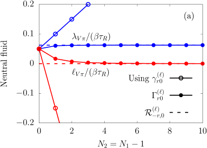
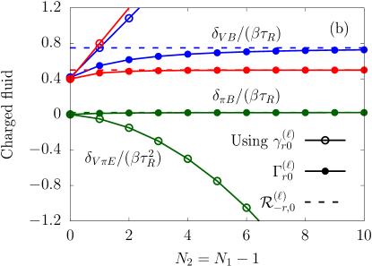
Figure 1: Dependence on $N_{2}=N_{1}-1$ of the coefficients (a) $\ell_{V\pi}=\tau_{V\pi}$, $\lambda_{V\pi}$ for a neutral fluid; and (b) $\delta_{V\pi E}$, $\delta_{VB}$, $\delta_{\pi B}$ for a charged fluid, computed using the approaches shown in Table 1.

.

IV.5 Transport coefficients for the ultrarelativistic ideal gas

We now employ the basis-free results (127),(128) for $\mathcal{R}^{(1)}_{-1,0}$, $\mathcal{R}^{(2)}_{-1,0}$, and $\mathcal{R}^{(2)}_{-2,0}$. The ultrarelativistic limit of the transport coefficients appearing in Eqs. (102)–(107) is then obtained as

$$\kappa =\frac{\beta P}{12}\,\tau_{V}\;,\quad\delta_{VV}=\tau_{V}\;,\quad\lambda_{VV}=\frac{3}{5}\,\tau_{V}\;,$$

$$\ell_{V\pi} =\tau_{V\pi}=0\;,\qquad\lambda_{V\pi}=\frac{\beta}{16}\,\tau_{V}\;.$$ (168)

Equations (108)–(112) reduce to

$$\eta=\frac{4P}{5}\,\tau_{\pi}\;,\quad\delta_{\pi\pi}=\frac{4}{3}\,\tau_{\pi}\;,\quad\tau_{\pi\pi}=\frac{10}{7}\,\tau_{\pi}\;,$$

$$\ell_{\pi V}=\tau_{\pi V}=\lambda_{\pi V}=0\;.$$ (169)

The coefficients in Eqs. (117)-(122) due to the electric and magnetic fields read

$$\delta_{VE} =\frac{\beta^{2}P}{12}\,\tau_{V}\;,\quad\delta_{\pi VE}=\frac{8}{5}\,\tau_{\pi}\;,$$

$$\delta_{\pi B} =\beta\tau_{\pi}\;,\quad\delta_{VB}=\frac{3\beta}{4}\,\tau_{V}\;,\qquad\delta_{V\pi E}=\frac{\beta^{2}}{48}\,\tau_{V}\;.$$ (170)

In the above, the coefficients involving the bulk viscous pressures were omitted.

For the ideal ultrarelativistic gas, Eq. (126) can be employed to show that

$$\frac{\partial\mathcal{R}^{(\ell)}_{r0}}{\partial\alpha}=0\;,\qquad\frac{\partial\mathcal{R}^{(\ell)}_{r0}}{\partial\beta}=-\frac{r}{\beta}\mathcal{R}^{(\ell)}_{r0}\;.$$ (171)

The above relations hold true also when $r<0$ and in particular also when $\mathcal{R}^{(\ell)}_{-r,0}$ is replaced by $\gamma^{(\ell)}_{r0}$ or $\Gamma^{(\ell)}_{r0}$, since their dependence on $\alpha$ and $\beta$ is identical to that of $\mathcal{R}^{(\ell)}_{-r,0}$. Thus, one can conclude that in all approaches mentioned here,

$$\tau_{V\pi}=\ell_{V\pi}\;,\qquad\lambda_{V\pi}=\frac{\tau_{V}}{16}\beta-\frac{\ell_{V\pi}}{4}\;.$$ (172)

Since the coefficients $\ell_{V\pi}$, $\tau_{V\pi}$, $\lambda_{V\pi}$, $\delta_{\pi B}$, $\delta_{VB}$, and $\delta_{V\pi E}$ involve $\mathcal{R}^{(1)}_{-1,0}$, $\mathcal{R}^{(2)}_{-1,0}$, and $\mathcal{R}^{(2)}_{-2,0}$, their values will differ between the various approaches discussed in the present section. All other transport coefficients assume the same values as in the standard DNMR approach. As pointed out in Table 1, when $N_{\ell}\rightarrow\infty$, the approach based on $\Gamma^{(\ell)}_{r0}$ converges to the basis-free one employing $\mathcal{R}^{(\ell)}_{-r,0}$. Conversely, the coefficients computed based on $\gamma^{(\ell)}_{r0}$ diverge with the truncation order $N_{\ell}$. We illustrate these behaviours in Fig. 1 for the coefficients shown in Table 1. Note that in the 14-moment approximation, when $N_{0}=2$, $N_{1}=1$, and $N_{2}=0$, the results obtained using the coefficients $\gamma^{(\ell)}_{r0}$ and $\Gamma^{(\ell)}_{r0}$ are identical and reproduce those reported in Refs. [33, 48].

V Shear-diffusion coupling: Longitudinal waves

In this section, we consider the propagation of longitudinal (sound) waves through an ultrarelativistic, uncharged ideal fluid. The purpose of this section is to compare the prediction of second-order fluid dynamics using the various expressions of the transport coefficients reported in Table 1 with that of kinetic theory in RTA. While the former can be estimated analytically, the latter is obtained numerically using the method described in Ref. [38]. Per definition, a sound wave is an infinitesimal perturbation, such that it is sufficient to consider the linear terms in the equations of motion. In the linearized equations of motion for an ultrarelativistic, uncharged fluid, only the coefficients $\ell_{V\pi},\ell_{\pi V}$ enter (as well as some coefficients in $\mathcal{K}^{\mu}$ and $\mathcal{K}^{\mu\nu}$, which, however, play no role in our investigation, see comment after Eq. (93)). Since $\ell_{\pi V}$ vanishes in all approaches considered here, we will refer only to the coefficient $\ell_{V\pi}$ listed in Table 1, for which we summarize the results below:

Basis-free: $$\ell_{V\pi} =0\;,$$ (173)

DNMR: $$\ell_{V\pi} =\frac{\beta}{20}(1-4N_{2})\tau_{V}\;,$$ (174)

Corrected DNMR: $$\ell_{V\pi} =\frac{6\beta(N_{2}+1)!}{(N_{2}+5)!}\,\tau_{V}\;.$$ (175)

In addition, we recall the result reported in Ref. [35], obtained using a second-order Chapman-Enskog approach:

$$\text{Ref.~{}\cite[cite]{[\@@bibref{Number}{Panda:2020zhr}{}{}]}:}\qquad\ell_{V\pi}=\frac{\beta}{4}\,\tau_{V}\;.$$ (176)

We note that the result $\ell_{V\pi}=0$ was also obtained in Ref. [50] using a Chapman-Enskog–like approach.

Since the corrected DNMR value lies between the DNMR (for $N_{2}=0$) and basis-free (for $N_{2}\rightarrow\infty$) results, we will not consider it explicitly in what follows. Instead, we will contrast the basis-free prediction to predictions due to Ref. [35] and to the DNMR prediction, where for illustrative purposes we choose $N_{2}=2$, leading to $\ell_{V\pi}=-7\beta\tau_{V}/20$.

This section is structured as follows. In Sec. V.1, we derive the equations of motion for sound waves. The resulting dispersion relations are computed in Sec. V.2. The analytical solutions and the numerical results are discussed in Sec. V.3.

V.1 Second-order equations for longitudinal waves

We assume that the background fluid is homogeneous and at rest, while the perturbations travel along the $z$ axis. The velocity of the perturbed fluid is $u^{\mu}=\gamma(1,0,0,\delta v)\simeq(1,0,0,\delta v)$, where $|\delta v|\ll 1$ is assumed to be small. For simplicity, the transverse motion leading to so-called shear waves is not taken into account. The properties of the background fluid are

$$e=e_{0}+\delta e\;,\qquad n=n_{0}+\delta n\;,$$ (177)

where again $|\delta e|/e_{0},|\delta n|/n_{0}\ll 1$. The diffusion vector $V^{\mu}$ and shear-stress tensor $\pi^{\mu\nu}$ can be described in terms of only two scalar quantities, $\delta V$ and $\delta\pi$, as follows:

$$V^{\mu}= \delta V(\delta v,0,0,1)\;,$$ (178)

and

$$\pi^{\mu\nu}= \delta\pi\begin{pmatrix}\delta v^{2}\gamma^{2}&0&0&\delta v\gamma^{2}\\ 0&-\frac{1}{2}&0&0\\ 0&0&-\frac{1}{2}&0\\ \delta v\gamma^{2}&0&0&\gamma^{2}\end{pmatrix}\;,$$ (179)

where the properties $u_{\mu}V^{\mu}=u_{\mu}\pi^{\mu\nu}=\pi^{\mu}{}_{\mu}=0$ were employed. Since both $\delta V$ and $\delta\pi$ are related to gradients of the fluid, they are of the same order of magnitude as the perturbations. In the linearized limit, $V^{\mu}$ and $\pi^{\mu\nu}$ reduce to

$$V^{\mu}\simeq\delta V(0,0,0,1)\;,\ \pi^{\mu\nu}\simeq\delta\pi\ {\rm diag}\left(0,-\frac{1}{2},-\frac{1}{2},1\right)\;.$$ (180)

Noting that the expansion scalar $\theta$ and the shear tensor $\sigma^{\mu\nu}$ reduce to

$$\theta=\partial_{z}\delta v\;,\qquad\sigma^{\mu\nu}={\rm diag}\left(0,\frac{1}{3},\frac{1}{3},-\frac{2}{3}\right)\partial_{z}\delta v\;,$$ (181)

while

$$\Delta^{\lambda}_{\mu}\nabla_{\nu}\pi^{\mu\nu}=\partial_{z}\pi^{\lambda z}=\delta^{\lambda}_{z}\partial_{z}\delta\pi\;,$$ (182)

the conservation equations (25)–(27) become

$$\partial_{t}\delta n+n_{0}\partial_{z}\delta v+\partial_{z}\delta V= 0\;,$$

$$\partial_{t}\delta e+(e_{0}+P_{0})\partial_{z}\delta v= 0\;,$$

$$(e_{0}+P_{0})\partial_{t}\delta v+\partial_{z}\delta P+\partial_{z}\delta\pi= 0\;.$$ (183)

The equations of motion for $\delta V$ and $\delta\pi$ can be obtained from Eqs. (89),(90) and (92),(93) by ignoring terms that are quadratic with respect to the perturbations:

$$\tau_{V}\dot{V}^{\langle\mu\rangle}+V^{\mu}= \kappa\nabla^{\mu}\alpha+\ell_{V\pi}\Delta^{\mu\nu}\nabla_{\lambda}\pi^{\lambda}_{\nu}\;,$$

$$\tau_{\pi}\dot{\pi}^{\langle\mu\nu\rangle}+\pi^{\mu\nu}= 2\eta\sigma^{\mu\nu}+\ell_{\pi V}\nabla^{\langle\mu}V^{\nu\rangle}\;.$$ (184)

Using $\dot{V}^{\langle\mu\rangle}\simeq\delta^{\mu}_{z}\partial_{t}\delta V$, $\dot{\pi}^{\langle zz\rangle}\simeq\partial_{t}\delta\pi$ and noting that $\ell_{\pi V}=0$ by virtue of Eq. (169), we find

$$\tau_{V}\partial_{t}\delta V+\delta V= -\kappa\partial_{z}\delta\alpha+\ell_{V\pi}\partial_{z}\delta\pi\;,$$

$$\tau_{\pi}\partial_{t}\delta\pi+\delta\pi= -\frac{4\eta}{3}\partial_{z}\delta v\;,$$ (185)

where $\delta\alpha=\frac{4}{n_{0}}\delta n-\frac{3}{P_{0}}\delta P$. We shall employ the Knudsen number ${\rm Kn}\sim|k\tau_{V}|,|k\tau_{\pi}|\ll 1$ for power-counting purposes in order to simplify some of the expressions appearing in the following sections.

V.2 Mode analysis

Now we perform the analysis of Eqs. (183) and (185) at the level of the Fourier modes corresponding to $e^{-i(\omega t-kz)}$, introduced for a quantity $A(t,x)$ as

$$A(t,x)=A_{0}+\int_{-\infty}^{\infty}dk\sum_{\omega}e^{-i(\omega t-kz)}\delta A_{\omega}(k)\;,$$ (186)

where $A_{0}$ is the constant background value of $A$, while $|k|=2\pi/\lambda$ is the wavenumber (not to be confused with the particle momentum $k^{\mu}$ from the previous sections) and $\omega\equiv\omega(k)$ is the angular frequency, whose real part gives rise to propagation. A negative imaginary part of $\omega$ leads to damping of the mode. A positive imaginary part would lead to an exponential increase and thus to an instability. Applying the above Fourier expansion leads to the matrix equation

$$\begin{pmatrix}-3\frac{\omega}{k}&4P_{0}&0&0&0\\ 1&-\frac{4\omega}{k}P_{0}&1&0&0\\ 0&\frac{4\eta}{3}&-\frac{i}{k}-\frac{\omega}{k}\tau_{\pi}&0&0\\ 0&n_{0}&0&-\frac{\omega}{k}&1\\ -\frac{3\kappa}{P_{0}}&0&-\ell_{V\pi}&\frac{4\kappa}{n_{0}}&-\frac{i}{k}-\frac{\omega}{k}\tau_{V}\end{pmatrix}\begin{pmatrix}\delta P_{\omega}(k)\\ \delta v_{\omega}(k)\\ \delta\pi_{\omega}(k)\\ \delta n_{\omega}(k)\\ \delta V_{\omega}(k)\end{pmatrix}\\ =0\;.$$ (187)

The modes supported by this system can be found by setting the determinant of the above matrix to $0$. Since $\ell_{\pi V}=0$, the $(\delta P,\delta v,\delta\pi)$ sector decouples from the $(\delta n,\delta V)$ sector and the determinant factorizes as

$$(k^{2}-3\omega^{2})(1-i\omega\tau_{\pi})-\frac{ik^{2}\omega}{P_{0}}\eta= 0\;,$$ (188)

$$\omega(1-i\omega\tau_{V})+\frac{4ik^{2}}{n_{0}}\kappa= 0\;.$$ (189)

The $(\delta P,\delta v,\delta\pi)$ sector contains the two sound or acoustic modes as well as a shear mode, while the $(\delta n,\delta V)$ sector contains a mode associated with particle-number transport (in the non-relativistic context called thermal mode) and a diffusive mode. While the sound modes and the thermal mode are hydrodynamic modes (i.e., the frequency vanishes for zero wavenumber), the shear and the diffusive modes are non-hydrodynamic modes (i.e., the frequency does not vanish for zero wavenumber).

Equations (188) and (189) agree with Eqs. (4.19) and (4.13) of Ref. [38] when identifying $\omega=-i\alpha$ and $\kappa=\lambda/16$. Therefore, the dispersion relations $\omega\equiv\omega(k)$ are identical to those identified in Eqs. (4.14) and (4.20)–(4.22) of Ref. [38]. Labeling the acoustic and shear modes as $\omega_{a}^{\pm}$ and $\omega_{\eta}$, respectively, we have

$$\omega^{\pm}_{a}=\pm|k|c_{s;a}-i\xi_{a},\qquad\omega_{\eta}=-i\xi_{\eta}\;,$$ (190)

where the argument $k$ was omitted for brevity. The quantities appearing above are defined as

$$c_{s;a}= \frac{1}{2|k|\tau_{\pi}\sqrt{3}}\left\{\frac{1}{R_{\eta}}\left[1-k^{2}\tau_{\pi}^{2}\left(1+\frac{\eta}{\tau_{\pi}P_{0}}\right)\right]-R_{\eta}\right\}\;,$$

$$\xi_{a}= \frac{1}{3\tau_{\pi}}\left\{1-\frac{1}{2R_{\eta}}\left[1-k^{2}\tau_{\pi}^{2}\left(1+\frac{\eta}{\tau_{\pi}P_{0}}\right)\right]-\frac{R_{\eta}}{2}\right\}\;,$$

$$\xi_{\eta}= \frac{1}{3\tau_{\pi}}\left\{1+\frac{1}{R_{\eta}}\left[1-k^{2}\tau_{\pi}^{2}\left(1+\frac{\eta}{\tau_{\pi}P_{0}}\right)\right]+R_{\eta}\right\}\;.$$ (191)

Here, the function $R_{\eta}$ is defined as

$$R_{\eta}= \begin{cases}R_{\eta}^{<},&\tau_{\pi}<\tau_{\pi,{\rm lim}}\;,\\ -R_{\eta}^{>},&\tau_{\pi}>\tau_{\pi;{\rm lim}}\;,\end{cases}$$

$$R_{\eta}^{<}= \left[1-3|k|\tau_{\pi}\sqrt{R_{\eta,{\rm aux}}}+3k^{2}\tau_{\pi}^{2}\left(1-\frac{\eta}{2P_{0}\tau_{\pi}}\right)\right]^{1/3}\;,$$

$$R_{\eta}^{>}= \left[-1+3|k|\tau_{\pi}\sqrt{R_{\eta,{\rm aux}}}-3k^{2}\tau_{\pi}^{2}\left(1-\frac{\eta}{2P_{0}\tau_{\pi}}\right)\right]^{1/3}\;,$$ (192)

with

$$R_{\eta,{\rm aux}}=1+\frac{2}{3}k^{2}\tau_{\pi}^{2}\left(1-\frac{5\eta}{2P_{0}\tau_{\pi}}-\frac{\eta^{2}}{8P_{0}^{2}\tau_{\pi}^{2}}\right)\\ +\frac{k^{4}\tau_{\pi}^{4}}{9}\left(1+\frac{\eta}{P_{0}\tau_{\pi}}\right)^{3}\;.$$ (193)

In the above, the value $\tau_{\pi,{\rm lim}}$ discerning between the two branches for $R_{\eta}$ is given by

$$\tau_{\pi,{\rm lim}}=\frac{1}{|k|}\left(1+\frac{\eta}{P_{0}\tau_{\pi}}\right)^{-1/2}\;,$$ (194)

where $\eta/(P_{0}\tau_{\pi})$ is independent of $\tau_{\pi}$ since $\eta\sim\tau_{\pi}$. Applying the power-counting scheme mentioned above, we observe that $c_{s;a}\simeq c_{s}+O({\rm Kn}^{2})$, with $c_{s}=1/\sqrt{3}$ the speed of sound, while $\xi_{a}\simeq\frac{k^{2}\eta}{6P_{0}}+O({\rm Kn}^{3})$, and $\xi_{\eta}\simeq\frac{1}{\tau_{\pi}}-\frac{k^{2}\eta}{3P_{0}}+O({\rm Kn}^{3})$.

The thermal and diffusive modes, $\omega^{-}_{\kappa}$ and $\omega^{+}_{\kappa}$, respectively, are

$$\omega^{\pm}_{\kappa}=-i\xi^{\pm}_{\kappa}\;,\,\,\xi^{\pm}_{\kappa}=\frac{1}{2\tau_{V}}\left(1\pm\sqrt{1-\frac{16k^{2}\kappa\tau_{V}}{n_{0}}}\right)\;,$$ (195)

and agree with Eq. (4.14) of Ref. [38]. A power-counting analysis reveals that $\xi^{-}_{\kappa}\simeq\frac{4k^{2}\kappa}{n_{0}}+O({\rm Kn}^{3})$ and $\xi^{+}_{\kappa}\simeq\frac{1}{\tau_{V}}-\frac{4k^{2}\kappa}{n_{0}}+O({\rm Kn}^{3})$.

With the dispersion relations at hand, we can now compute the mode amplitudes. Focusing first on the thermal and diffusive modes, it is not difficult to see that $\delta P^{\pm}_{\kappa}(k)=\delta v^{\pm}_{\kappa}(k)=\delta\pi^{\pm}_{\kappa}(k)=0$, while the amplitude of the diffusion current can be linked to that of the density fluctuations via

$$\delta V^{\pm}_{\kappa}(k)=-\frac{i\xi^{\pm}_{\kappa}}{k}\delta n^{\pm}_{\kappa}(k)\;.$$ (196)

In the sound and shear sector, the amplitude of the pressure fluctuations can be defined as an independent variable, while the other amplitudes can be expressed as

$$\delta v_{\omega}(k) =\frac{3\omega}{4kP_{0}}\delta P_{\omega}(k)\;,\quad\delta\pi_{\omega}(k)=\left(\frac{3\omega^{2}}{k^{2}}-1\right)\delta P_{\omega}(k)\;,$$

$$\delta n_{\omega}(k) =\left[\frac{3n_{0}}{4P_{0}}+\frac{i\ell_{V\pi}(3\omega^{2}-k^{2})}{\frac{4ik^{2}\kappa}{n_{0}}+\omega(1-i\omega\tau_{V})}\right]\delta P_{\omega}(k)\;,$$

$$\delta V_{\omega}(k) =\frac{i\omega}{k}\frac{\ell_{V\pi}(3\omega^{2}-k^{2})}{\frac{4ik^{2}\kappa}{n_{0}}+\omega(1-i\omega\tau_{V})}\delta P_{\omega}(k)\;,$$ (197)

where $\omega$ is either $\omega_{a}^{\pm}$ or $\omega_{\eta}$. From the above, it is clear that a non-vanishing value of $\ell_{V\pi}$ introduces acoustic and shear modes into the diffusion current, allowing the diffusion current to propagate by means of the sound modes. Thus, the basis-free result $\ell_{V\pi}=0$ can be distinguished from the Chapman-Enskog and DNMR results $\ell_{V\pi}\neq 0$ by considering the propagation of a simple harmonic wave, which we discuss below.

V.3 Numerical results

At initial time $t_{0}=0$, we consider

$$n(t_{0},z)=n_{0}\;,\ P(t_{0},z)=P_{0}+\delta P\cos(kz)\;,$$ (198)

while $\delta v(t_{0},x)=\delta\pi(t_{0},z)=\delta V(t_{0},z)=0$. This initial state can be implemented by setting

$$\delta P_{\omega}(k^{\prime})=\frac{\delta P_{\omega}}{2}[\delta(k^{\prime}-k)+\delta(k^{\prime}+k)],$$ (199)

with $\sum_{\omega}\delta P_{\omega}=\delta P$. This allows the solutions for $\delta P(t,z)$, $v(t,z)$, and $\delta\pi(t,z)$ to be written as

$$\delta P(t,z)= \cos(kz)\sum_{\omega^{\pm}_{a},\omega_{\eta}}\delta P_{\omega}e^{-i\omega t}\;,$$

$$\delta v(t,z)= \frac{3i}{4kP_{0}}\sin(kz)\sum_{\omega^{\pm}_{a},\omega_{\eta}}\omega\delta P_{\omega}e^{-i\omega t}\;,$$

$$\delta\pi(t,z)= \cos(kz)\sum_{\omega^{\pm}_{a},\omega_{\eta}}\left(\frac{3\omega^{2}}{k^{2}}-1\right)\delta P_{\omega}e^{-i\omega t}\;.$$ (200)

Imposing the initial conditions from Eq. (198) leads to

$$\sum_{\omega^{\pm}_{a},\omega_{\eta}}\delta P_{\omega}=\delta P\;,\quad\sum_{\omega^{\pm}_{a},\omega_{\eta}}\omega\delta P_{\omega}=0\;,$$

$$\sum_{\omega^{\pm}_{a},\omega_{\eta}}\omega^{2}\delta P_{\omega}=\frac{k^{2}}{3}\delta P\;,$$ (201)

which admits the solutions

$$\delta P_{a}^{\pm}= \pm\frac{k^{2}+3\omega_{\eta}\omega_{a}^{\mp}}{6|k|c_{s;a}(\omega_{a}^{\pm}-\omega_{\eta})}\delta P\;,$$

$$\delta P_{\eta}= -\frac{k^{2}(1-3c_{s;a}^{2})-3\xi_{a}^{2}}{3[k^{2}c_{s;a}^{2}+(\xi_{a}-\xi_{\eta})^{2}]}\delta P\;.$$ (202)

For small ${\rm Kn}$, we have

$$\delta P_{a}^{\pm}= \frac{\delta P}{2}\pm\frac{i|k|\eta c_{s}}{4P_{0}}\delta P+O({\rm Kn}^{3})\;,$$

$$\delta P_{\eta}= \frac{k^{4}\eta\tau_{\pi}^{3}}{9P_{0}}\delta P+O({\rm Kn}^{6})\;.$$ (203)

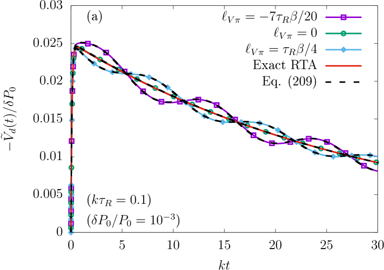
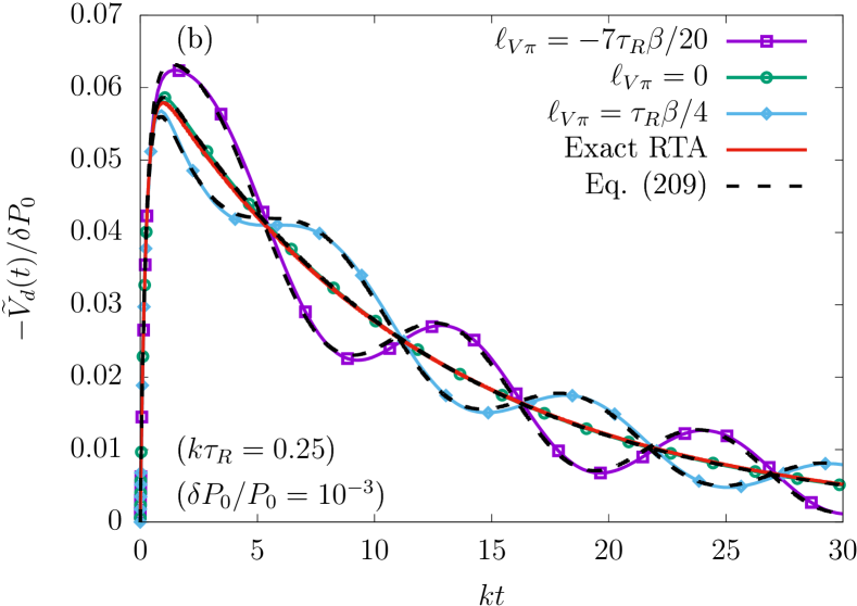
Figure 2: Time evolution of $-\widetilde{V}_{d}(t)/\delta P_{0}$ for the initial conditions in Eq. (198). The numerical solutions of the linearized equations (183) and (185) are shown using lines and symbols for various values of $\ell_{V\pi}$. The dashed black lines show their approximate analytical solution given in Eq. (209). The numerical solution of the Boltzmann equation in RTA is shown with the solid red line. All results are obtained for $k\tau_{R}=0.1$ (a) and $0.25$ (b) and we considered $\delta P_{0}/P_{0}=10^{-3}$.

To correctly assess the role of $\ell_{V\pi}$, we first note that for the shear mode, the factor $1-i\omega_{\eta}\tau_{V}\simeq 1-\frac{\tau_{V}}{\tau_{\pi}}+O({\rm Kn}^{2})$. For $\tau_{V}=\tau_{\pi}=\tau_{R}$, this is of order $O({\rm Kn}^{2})$, while it is of order $O({\rm Kn}^{0})$ when $\tau_{V}\neq\tau_{\pi}$. Focusing now on the particle-number fluctuations, we may write $\delta n_{\omega}(k^{\prime})=\frac{\delta n_{\omega}}{2}[\delta(k^{\prime}-k)+\delta(k^{\prime}+k)]$, where the amplitude of the corresponding acoustic and shear modes are obtained up to second order in ${\rm Kn}$ as

$$\delta n_{a}^{\pm} \simeq\frac{n_{0}}{2P_{0}}\left(\frac{3}{4}\pm\frac{3i|k|c_{s}}{8P_{0}}\eta+\frac{k^{2}}{n_{0}}\ell_{V\pi}\eta\right)\delta P\;,$$

$$\delta n_{\eta} \simeq\frac{k^{2}\tau_{R}n_{0}}{n_{0}\eta-12P_{0}\kappa}\ell_{V\pi}\eta\delta P\;.$$ (204)

For the diffusion current, we write $\delta V_{\omega}(k^{\prime})=-\frac{i\delta V_{\omega}}{2}[\delta(k^{\prime}-k)-\delta(k^{\prime}+k)]$, where

$$\delta V_{a}^{\pm} \simeq\pm\frac{ik^{3}c_{s}\delta P}{2P_{0}|k|}\ell_{V\pi}\eta\;, \delta V_{\eta} \simeq\frac{kn_{0}\delta P}{n_{0}\eta-12P_{0}\kappa}\ell_{V\pi}\eta\;.$$ (205)

The amplitudes of the thermal and diffusive modes $\delta n^{\pm}_{\kappa}$ can be found by noting that

$$\delta n(t_{0},z)\simeq \cos(kz)\left[\frac{3n_{0}\delta P}{4P_{0}}+\delta n^{+}_{\kappa}+\delta n^{-}_{\kappa}\right.$$

$$\left.+\left(1+\frac{\tau_{R}n_{0}P_{0}}{n_{0}\eta-12P_{0}\kappa}\right)\frac{k^{2}}{P_{0}}\ell_{V\pi}\eta\delta P\right]\;,$$

$$\delta V(t_{0},z)\simeq \frac{\sin(kz)}{k}\left(\frac{k^{2}n_{0}\ell_{V\pi}\eta\delta P}{n_{0}\eta-12P_{0}\kappa}+\xi^{+}_{\kappa}\delta n^{+}_{\kappa}+\xi^{-}_{\kappa}\delta n^{-}_{\kappa}\right)\;,$$ (206)

where only terms up to second order with respect to ${\rm Kn}$ were shown. Imposing $\delta n(t_{0},z)=V_{d}(t_{0},z)=0$ gives

$$\delta n_{\kappa}^{\pm}\simeq\pm\frac{n_{0}\xi^{\mp}\delta P}{P_{0}(\xi^{+}_{\kappa}-\xi^{-}_{\kappa})}\left(\frac{3}{4}+\frac{\tau_{R}k^{2}P_{0}\ell_{V\pi}\eta}{n_{0}\eta-12P_{0}\kappa}+\frac{k^{2}}{n_{0}}\ell_{V\pi}\eta\right)\\ \mp\frac{k^{2}n_{0}}{(n_{0}\eta-12P_{0}\kappa)(\xi^{+}_{\kappa}-\xi^{-}_{\kappa})}\ell_{V\pi}\eta\delta P\;,$$ (207)

while $\delta V^{\pm}_{\kappa}=\xi^{\pm}_{\kappa}\delta n^{\pm}_{\kappa}/k$. Noting that

$$\xi^{+}_{\kappa}\xi^{-}_{\kappa}=\frac{4k^{2}\kappa}{n_{0}\tau_{R}}\;,\quad\xi^{+}_{\kappa}-\xi^{-}_{\kappa}=\frac{1}{\tau_{R}}\sqrt{1-\frac{16k^{2}\kappa\tau_{R}}{n_{0}}}\;,$$ (208)

we obtain $\delta V(t,z)$ as

$$\delta V(t,z)\simeq\frac{kn_{0}\delta P}{P_{0}}\sin(kz)\Bigg{[}\frac{|k|}{n_{0}}c_{s}\ell_{V\pi}\eta e^{-\xi_{a}t}\sin(kc_{s;a}t)\\ +\frac{P_{0}\ell_{V\pi}\eta}{n_{0}\eta-12P_{0}\kappa}\left(e^{-\xi_{\eta}t}-\tau_{R}\frac{\xi^{+}_{\kappa}e^{-\xi^{+}_{\kappa}t}-\xi^{-}_{\kappa}e^{-\xi^{-}_{\kappa}t}}{\sqrt{1-\frac{16k^{2}\kappa}{n_{0}}\tau_{R}}}\right)\\ +\frac{\kappa}{n_{0}}\left(3+\frac{4\tau_{R}k^{2}P_{0}\ell_{V\pi}\eta}{n_{0}\eta-12P_{0}\kappa}+\frac{4k^{2}}{n_{0}}\ell_{V\pi}\eta\right)\frac{e^{-\xi^{+}_{\kappa}t}-e^{-\xi^{-}_{\kappa}t}}{\sqrt{1-\frac{16k^{2}\kappa}{n_{0}}\tau_{R}}}\Bigg{]}\;.$$ (209)

It can be seen that $\ell_{V\pi}$ introduces an oscillatory piece in the diffusion current. In order to facilitate the analysis, we introduce the amplitudes $\widetilde{\delta e}$, $\widetilde{\delta v}$, $\widetilde{\delta\pi}$, $\widetilde{\delta n}$, and $\widetilde{\delta V}$ via

$$\begin{pmatrix}\widetilde{\delta e}(t)\\ \widetilde{\delta\pi}(t)\\ \widetilde{\delta n}(t)\end{pmatrix}= \frac{k}{\pi}\int_{0}^{2\pi/k}dz\begin{pmatrix}\delta e(t,z)\\ \delta\pi(t,z)\\ \delta n(t,z)\end{pmatrix}\cos(kz)\;,$$ (210)

$$\begin{pmatrix}\widetilde{\delta v}(t)\\ \widetilde{\delta V}(t)\end{pmatrix}= \frac{k}{\pi}\int_{0}^{2\pi/k}dz\begin{pmatrix}\delta v(t,z)\\ \delta V(t,z)\end{pmatrix}\sin(kz)\;.$$ (211)

The linearized equations (183) and (185) are then solved as a set of ODEs by replacing

$$\partial_{z}\left(\delta e,\delta v,\delta\pi,\delta n,\delta V\right)\rightarrow k\left(-\widetilde{\delta e},\widetilde{\delta v},-\widetilde{\delta\pi},-\widetilde{\delta n},\widetilde{\delta V}\right)\;.$$ (212)

Figure 2 shows the results obtained using the values of $\ell_{V\pi}=-7\beta\tau_{R}/20$, $0$, and $\beta\tau_{R}/4$, as given by the DNMR approach based on $\gamma^{(2)}_{1}$ with $N_{2}=2$ (174), the basis-free approach (173), and in Ref. [35], respectively. The numerical results are compared with the analytical prediction (209), shown with dashed black lines. The small discrepancies seen in panel (b) are due to the approximations made in deriving Eq. (209). Additionally, we also show with the solid red line the numerical solution of the Boltzmann equation (1) with the Anderson-Witting collision model (53), obtained as described in Ref. [38]. The basis-free and RTA results are in excellent agreement, confirming that for the RTA, $\ell_{V\pi}=0$.

VI Conclusions

In this paper, we computed the transport coefficients of second-order relativistic fluid dynamics from the relativistic Boltzmann equation in the relaxation-time approximation (RTA) of the collision term.

Employing the method of moments, the irreducible moments for a negative power of energy, the so-called negative-order moments, are usually expressed in terms of the ones with a non-negative power of energy using a kind of completeness relation, which becomes exact in the limit when the truncation order $N_{\ell}\rightarrow\infty$. Focusing on the 14-dynamical moments approximation, we then considered different approaches to relate the negative-order moments $\rho_{-r}^{\mu_{1}\cdots\mu_{\ell}}$ to the zeroth-order ones: (i) the original DNMR approach [33], which features the coefficients $\gamma^{(\ell)}_{r0}$, cf. Eq. (45), (ii) a corrected DNMR approach [37], which employs the coefficients $\Gamma^{(\ell)}_{r0}$ of Eq. (47), (iii) a so-called shifted-basis approach, which includes a certain set of negative-order moments in the expansion basis, cf. Eq. (52), and (iv) a basis-free approach tailored to the RTA, cf. Eq. (64).

The shifted-basis approach acknowledges the importance of the negative-order moments by including them explicitly in the expansion basis. The magnitude of the shifts $s_{\ell}$ for the irreducible moments of tensor rank $\ell$ are defined by the lowest-order moment $\rho^{\mu_{1}\cdots\mu_{\ell}}_{-s_{\ell}}$, which must be explicitly accounted for in the expansion. Setting $s_{\ell}=2$ for the $m_{0}>0$ case and $s_{\ell}=\ell$ when $m_{0}=0$ leads to perfect agreement with the basis-free approach.

Furthermore, we checked our results for consistency by employing the Chapman-Enskog approach presented in Ref. [18]. Using the properties of the RTA collision model, we showed that the Chapman-Enskog method and the method of moments are equivalent up to second order. We also showed that the discrepancies reported in Ref. [34, 35] are due to the omission of second-order contributions in these latter references.

In the context of an ultrarelativistic ideal gas, we computed $\gamma^{(\ell)}_{r0}$ and $\Gamma^{(\ell)}_{r0}$ explicitly for $\ell=1$, $2$ and $r=1$, $2$. We showed that $\gamma^{(\ell)}_{r0}$ and all transport coefficients that depend on it, i.e., $\ell_{V\pi}$, $\tau_{V\pi}$, $\lambda_{V\pi}$, as well as $\delta_{\pi B}$, $\delta_{VB}$, $\delta_{V\pi E}$, diverge with the truncation order $N_{\ell}$. Even though the coefficients $\Gamma^{(\ell)}_{r0}$ also depend explicitly on $N_{\ell}$, they converge towards the basis-free results when $N_{\ell}\rightarrow\infty$.

Finally, we validated our results in the context of longitudinal waves propagating through an ultrarelativistic ideal gas. Our result $\ell_{V\pi}=0$ for the coefficient responsible for the coupling to the shear-stress tensor in the equation for the diffusion current is in perfect agreement with numerical simulations of the RTA kinetic equation.

Appendix A Second-order Chapman-Enskog method

Recalling the notation introduced in Refs. [34, 35], the distribution function is written as $f_{\mathbf{k}}=f_{0{\mathbf{k}}}+\delta f^{(1)}_{\mathbf{k}}+\delta f^{(2)}_{\mathbf{k}}$. The correction $\delta f^{(i)}$ is obtained as

$$\delta f^{(i)}_{\mathbf{k}}=\left(-\frac{\tau_{R}}{E_{\mathbf{k}}}k^{\mu}\partial_{\mu}\right)^{i}f_{0{\mathbf{k}}}\;.$$ (213)

Due to the expansion of the comoving derivative $D=\sum_{j=0}^{\infty}\varepsilon^{j}D_{j}$ in Eq. (71), it is clear that $\delta f^{(i)}_{\mathbf{k}}$ contains contributions of order $i$, $i+1$, …. This should be contrasted with the expansion in Eq. (69), where $\varepsilon f_{\mathbf{k}}^{(1)}$ and $\varepsilon^{2}f_{\mathbf{k}}^{(2)}$ contain solely terms of first and second order with respect to $\varepsilon$, respectively, see Eqs. (75) and (76).

For example, using Eq. (213) together with Eq. (71) to compute $\delta f^{(1)}_{\mathbf{k}}$, it becomes clear that it can be written in terms of $\varepsilon f_{\mathbf{k}}^{(1)}$ and higher-order contributions as

$$\delta f^{(1)}_{\mathbf{k}} =\varepsilon f^{(1)}_{\mathbf{k}}-\tau_{R}\sum_{i=1}^{\infty}\varepsilon^{i}D_{i}f_{0{\mathbf{k}}}$$

$$=\varepsilon f^{(1)}_{\mathbf{k}}-\varepsilon\tau_{R}D_{1}f_{0{\mathbf{k}}}+O(\varepsilon^{3})\;,$$ (214)

where we recall that $\tau_{R}$ is of the same order as the book-keeping parameter $\varepsilon$. The second-order term $\delta f^{(2)}_{\mathbf{k}}$ can be obtained as

$$\delta f^{(2)}_{{\mathbf{k}}}=\varepsilon^{2}f^{(2)}_{\mathbf{k}}+\varepsilon\tau_{R}D_{1}f_{0{\mathbf{k}}}+O(\varepsilon^{3})\;,$$ (215)

where the second term on the right-hand side makes also a second-order contribution, being explicitly given by

$$D_{1}f_{0{\mathbf{k}}}=f_{0{\mathbf{k}}}\bar{f}_{0{\mathbf{k}}}\left[D_{1}\alpha-E_{\mathbf{k}}D_{1}\beta-\beta k^{\langle\mu\rangle}D_{1}u_{\mu}\right]\;.$$ (216)

The discrepancy between the results derived in the present paper and those reported in Refs. [34, 35] arises because the second-order contribution $-\varepsilon\tau_{R}D_{1}f_{0{\mathbf{k}}}$ to $\delta f^{(1)}_{\mathbf{k}}$ was neglected in these latter references. Due to this omission, the resulting distribution function reads

$$\hat{f}_{\mathbf{k}} \equiv f_{0{\mathbf{k}}}+(\delta f^{(1)}_{\mathbf{k}}+\varepsilon\tau_{R}D_{1}f_{0{\mathbf{k}}})+\delta f^{(2)}_{\mathbf{k}}+O(\varepsilon^{3})$$

$$=f_{\mathbf{k}}+\varepsilon\tau_{R}D_{1}f_{0{\mathbf{k}}}+O(\varepsilon^{3})\;,$$ (217)

where $f_{\mathbf{k}}=f_{0{\mathbf{k}}}+\varepsilon f^{(1)}_{\mathbf{k}}+\varepsilon^{2}f^{(2)}_{\mathbf{k}}$. In the above and henceforth, we use an overhead hat $\hat{f}_{\mathbf{k}}$ to denote quantities that arise when the $-\varepsilon\tau_{R}D_{1}f_{0{\mathbf{k}}}$ term is omitted from $\delta f^{(1)}_{\mathbf{k}}$, as considered in Refs. [34, 35]. Using Eqs. (79)–(80) with $f_{\mathbf{k}}^{(i)}$ and $\hat{f}_{\mathbf{k}}^{(i)}$, we can evaluate the difference $\rho_{r}^{\mu_{1}\cdots\mu_{\ell}}-\hat{\rho}_{r}^{\mu_{1}\cdots\mu_{\ell}}$ at second order as

$$\rho_{r}^{\mu_{1}\cdots\mu_{\ell}}-\hat{\rho}_{r}^{\mu_{1}\cdots\mu_{\ell}}\simeq-\varepsilon\tau_{R}\int dK\,E_{\mathbf{k}}^{r}k^{\langle\mu_{1}}\cdots k^{\mu_{\ell}\rangle}D_{1}f_{0{\mathbf{k}}}\;.$$ (218)

In the case of the scalar moments, we find

$$\rho_{0}-\hat{\rho}_{0} =-\tau_{R}\frac{G_{20}}{D_{20}}(\Pi\theta-\pi^{\mu\nu}\sigma_{\mu\nu})$$

$$-\tau_{R}\frac{G_{30}}{D_{20}}(V^{\mu}\dot{u}_{\mu}-\nabla_{\mu}V^{\mu})+O(\varepsilon^{3})\;,$$ (219)

$$\rho_{1}-\hat{\rho}_{1} =-\tau_{R}(V^{\mu}\dot{u}_{\mu}-\nabla_{\mu}V^{\mu})+O(\varepsilon^{3})\;,$$ (220)

$$\rho_{2}-\hat{\rho}_{2} =\tau_{R}(\Pi\theta-\pi^{\mu\nu}\sigma_{\mu\nu})+O(\varepsilon^{3})\;,$$ (221)

where (74) was employed to replace $D_{1}\alpha$ and $D_{1}\beta$. Since $\rho_{1}=\rho_{2}=0$ according to Eqs. (11)–(12), it can be seen that $\hat{\rho}_{1}$ and $\hat{\rho}_{2}$ will in general not vanish. By the same reason, a non-vanishing energy-momentum flow $W^{\mu}=\rho_{1}^{\mu}$ appears:

$$\rho^{\mu}_{1}-\hat{\rho}^{\mu}_{1}=-\tau_{R}\left(\nabla^{\mu}\Pi-\Delta^{\mu}_{\alpha}\nabla_{\beta}\pi^{\alpha\beta}-\Pi\dot{u}^{\mu}+\pi^{\mu\nu}\dot{u}_{\nu}\right)\\ +O(\varepsilon^{3})\;.$$ (222)

Equations (220)–(222) show that due to second-order inconsistencies, the Landau matching conditions (11), (12) and the Landau frame (10) are no longer satisfied, hence violating the conservation of particle number and energy-momentum in the RTA.

The dissipative quantities also show discrepancies,

$$\Pi-\hat{\Pi} =\frac{\tau_{R}n}{\beta D_{20}}(hJ_{10}-J_{20})(\Pi\theta-\pi^{\mu\nu}\sigma_{\mu\nu})$$ (223)

$$+\frac{\tau_{R}n}{\beta D_{20}}(hJ_{20}-J_{30})(V^{\mu}\dot{u}_{\mu}-\nabla_{\mu}V^{\mu})+O(\varepsilon^{3})\;,$$

$$V^{\mu}-\hat{V}^{\mu} =-\frac{\tau_{R}}{h}\left(\nabla^{\mu}\Pi-\Delta^{\mu}_{\alpha}\nabla_{\beta}\pi^{\alpha\beta}-\Pi\dot{u}^{\mu}+\pi^{\mu\nu}\dot{u}_{\nu}\right)$$

$$+O(\varepsilon^{3})\;,$$ (224)

while $\pi^{\mu\nu}-\hat{\pi}^{\mu\nu}=O(\varepsilon^{3})$. From the above relations, it can be seen that the transport coefficients $\delta_{\Pi\Pi}$, $\lambda_{\Pi\pi}$, $\tau_{\Pi V}$, $\ell_{\Pi V}$, $\ell_{V\Pi}$, $\ell_{V\pi}$, $\tau_{V\Pi}$, and $\tau_{V\pi}$ are modified as follows:

$$\begin{pmatrix}\delta_{\Pi\Pi}\\ \lambda_{\Pi\pi}\end{pmatrix} =\begin{pmatrix}\hat{\delta}_{\Pi\Pi}\\ \hat{\lambda}_{\Pi\pi}\end{pmatrix}-\frac{\tau_{R}n}{\beta D_{20}}(hJ_{10}-J_{20})\;,$$ (225)

$$\begin{pmatrix}\tau_{\Pi V}\\ -\ell_{\Pi V}\end{pmatrix} =\begin{pmatrix}\hat{\tau}_{\Pi V}\\ -\hat{\ell}_{\Pi V}\end{pmatrix}-\frac{\tau_{R}n}{\beta D_{20}}(hJ_{20}-J_{30})\;,$$ (226)

$$\begin{pmatrix}\ell_{V\Pi}\\ \ell_{V\pi}\\ \tau_{V\Pi}\\ \tau_{V\pi}\end{pmatrix} =\begin{pmatrix}\hat{\ell}_{V\Pi}\\ \hat{\ell}_{V\pi}\\ \hat{\tau}_{V\Pi}\\ \hat{\tau}_{V\pi}\end{pmatrix}+\frac{\tau_{R}}{h}\;.$$ (227)

References

- Banyuls et al. [1997] F. Banyuls, J. A. Font, J. M. Ibanez, J. M. Martí, and J. A. Miralles, Numerical general relativistic hydrodynamics: A local characteristic approach, Astrophys. J. 476, 221 (1997).
- Begelman et al. [1984] M. C. Begelman, R. D. Blandford, D. Roger, and M. J. Rees, Theory of extragalactic radio sources, Rev. Mod. Phys. 56 56, 255 (1984).
- Fryer [2004] C. L. Fryer, Stellar Collapse (Springer Dordrecht, 2004).
- Martí and Müller [2015] J. M. Martí and E. Müller, Grid-based methods in relativistic hydrodynamics and magnetohydrodynamics, Living Rev. Comput. Astrophys. 1, 3 (2015).
- Kouveliotou et al. [2012] C. Kouveliotou, R. A. M. Wijers, and S. Woosley, Gamma-ray bursts (Cambridge University Press, New York, NY, 2012).
- Ellis et al. [2012] G. F. R. Ellis, R. Maartens, and M. A. H. MacCallum, Relativistic cosmology (Cambridge University Press, Cambridge, UK, 2012).
- Muronga [2002] A. Muronga, Second order dissipative fluid dynamics for ultrarelativistic nuclear collisions, Phys. Rev. Lett. 88, 062302 (2002), [Erratum: Phys.Rev.Lett. 89, 159901 (2002)], arXiv:nucl-th/0104064 .
- Csernai et al. [2006] L. P. Csernai, J. I. Kapusta, and L. D. McLerran, On the Strongly-Interacting Low-Viscosity Matter Created in Relativistic Nuclear Collisions, Phys. Rev. Lett. 97, 152303 (2006), arXiv:nucl-th/0604032 .
- Romatschke and Romatschke [2007] P. Romatschke and U. Romatschke, Viscosity Information from Relativistic Nuclear Collisions: How Perfect is the Fluid Observed at RHIC?, Phys. Rev. Lett. 99, 172301 (2007), arXiv:0706.1522 [nucl-th] .
- Heinz and Snellings [2013] U. Heinz and R. Snellings, Collective flow and viscosity in relativistic heavy-ion collisions, Ann. Rev. Nucl. Part. Sci. 63, 123 (2013), arXiv:1301.2826 [nucl-th] .
- Bernhard et al. [2019] J. E. Bernhard, J. S. Moreland, and S. A. Bass, Bayesian estimation of the specific shear and bulk viscosity of quark–gluon plasma, Nature Phys. 15, 1113 (2019).
- Auvinen et al. [2020] J. Auvinen, K. J. Eskola, P. Huovinen, H. Niemi, R. Paatelainen, and P. Petreczky, Temperature dependence of of strongly interacting matter: Effects of the equation of state and the parametric form of , Phys. Rev. C 102, 044911 (2020), arXiv:2006.12499 [nucl-th] .
- Müller [1967] I. Müller, Zum paradoxon der wärmeleitungstheorie, Z. Phys. 198, 329 (1967).
- Israel and Stewart [1979] W. Israel and J. M. Stewart, Transient relativistic thermodynamics and kinetic theory, Ann. Phys. 118, 341 (1979).
- de Groot et al. [1980] S. R. de Groot, W. A. van Leeuwen, and C. G. van Weert, Relativistic kinetic theory: Principles and applications (North-Holland Publ. Comp, Amsterdam, 1980).
- Hiscock and Lindblom [1983] W. A. Hiscock and L. Lindblom, Stability and causality in dissipative relativistic fluids, Ann. Phys. 151, 466 (1983).
- Hiscock and Lindblom [1985] W. A. Hiscock and L. Lindblom, Generic instabilities in first-order dissipative relativistic fluid theories, Phys. rev. D 31, 725 (1985).
- Cercignani and Kremer [2002] C. Cercignani and G. M. Kremer, The Relativistic Boltzmann Equation: Theory and Applications (Springer, 2002).
- Rezzolla and Zanotti [2013] L. Rezzolla and O. Zanotti, Relativistic Hydrodynamics (Oxford University Press, Oxford, United Kingdom, 2013).
- Chapman and Cowling [1991] S. Chapman and T. G. Cowling, The mathematical theory of non-uniform gases, 3rd ed. (Cambridge University Press, 1991).
- Chapman and Cowling [1988] S. Chapman and T. G. Cowling, The Boltzmann equation and its applications, 1st ed. (Springer, 1988).
- Struchtrup [2004] H. Struchtrup, Stable transport equations for rarefied gases at high orders in the knudsen number, Phys. Fluids 16, 3921 (2004).
- Grad [1949] H. Grad, On the kinetic theory of rarefied gases, Commun. Pure Appl. Math. 2, 331 (1949).
- Bhatnagar et al. [1954] P. L. Bhatnagar, E. P. Gross, and M. Krook, A model for collision processes in gases. I. Small amplitude processes in charged and neutral one-component systems, Phys. Rev. 94, 511 (1954).
- Marle [1969] C. Marle, Sur l’établissement des équations de l’hydrodynamique des fluides relativistes dissipatifs. I. - L’équation de Boltzmann relativiste, Annales de l’I. H. P. Physique théorique 10, 67 (1969).
- Anderson and Witting [1974] J. L. Anderson and H. R. Witting, A relativistic relaxation-time for the Boltzmann equation, Physica 74, 466 (1974).
- Florkowski et al. [2013] W. Florkowski, R. Ryblewski, and M. Strickland, Testing viscous and anisotropic hydrodynamics in an exactly solvable case, Phys. Rev. C 88, 024903 (2013).
- Florkowski et al. [2014] W. Florkowski, E. Maksymiuk, R. Ryblewski, and M. Strickland, Exact solution of the (0+1)-dimensional Boltzmann equation for a massive gas, Phys. Rev. C 89, 054908 (2014), arXiv:1402.7348 [hep-ph] .
- Denicol et al. [2014] G. S. Denicol, U. Heinz, M. Martinez, J. Noronha, and M. Strickland, New Exact Solution of the Relativistic Boltzmann Equation and its Hydrodynamic Limit, Phys. Rev. Lett. 113, 202301 (2014).
- Bazow et al. [2016] D. Bazow, G. S. Denicol, U. Heinz, M. Martinez, and J. Noronha, Analytic solution of the Boltzmann equation in an expanding system, Phys. Rev. Lett. 116, 022301 (2016).
- Denicol and Noronha [2019] G. S. Denicol and J. Noronha, Hydrodynamic attractor and the fate of perturbative expansions in Gubser flow, Phys. Rev. D 99, 116004 (2019).
- McNelis et al. [2021] M. McNelis, D. Bazow, and U. Heinz, Anisotropic fluid dynamical simulations of heavy-ion collisions, Comput. Phys. Commun. 267, 108077 (2021).
- Denicol et al. [2012] G. S. Denicol, H. Niemi, E. Molnar, and D. H. Rischke, Derivation of transient relativistic fluid dynamics from the boltzmann equation, Phys. Rev. D 85, 114047 (2012).
- Jaiswal [2013] A. Jaiswal, Relativistic dissipative hydrodynamics from kinetic theory with relaxation time approximation, Phys. Rev. C 87, 051901 (2013), arXiv:1302.6311 [nucl-th] .
- Panda et al. [2021a] A. K. Panda, A. Dash, R. Biswas, and V. Roy, Relativistic non-resistive viscous magnetohydrodynamics from the kinetic theory: a relaxation time approach, JHEP 03, 216, arXiv:2011.01606 [nucl-th] .
- Panda et al. [2021b] A. K. Panda, A. Dash, R. Biswas, and V. Roy, Relativistic resistive dissipative magnetohydrodynamics from the relaxation time approximation, Phys. Rev. D 104, 054004 (2021b), arXiv:2104.12179 [nucl-th] .
- Wagner et al. [2022] D. Wagner, A. Palermo, and V. E. Ambruş, Inverse-Reynolds-dominance approach to transient fluid dynamics, Phys. Rev. D 106, 016013 (2022), arXiv:2203.12608 [nucl-th] .
- Ambru\cbs [2018] V. E. Ambru\cbs, Transport coefficients in ultrarelativistic kinetic theory, Phys. Rev. C 97, 024914 (2018).
- Jüttner [1911] F. Jüttner, Das maxwellsche gesetz der geschwindigkeitsverteilung in der relativtheorie, Ann. Phys. 339, 856 (1911).
- Landau and E.M.Lifshitz [1987] L. Landau and E.M.Lifshitz, Fluid Dynamics, 2nd edition (Butterworth-Heinemann, 1987).
- Thorne [1981] K. S. Thorne, Relativistic radiative transfer: moment formalisms, Mon. Not. R. Astron. Soc. 194, 439 (1981).
- Struchtrup [1998] H. Struchtrup, Projected moments in relativistic kinetic theory, Physica A 253, 555 (1998).
- Eu [2016] B. C. Eu, Kinetic Theory of Nonequilibrium Ensembles, Irreversible Thermodynamics, and Generalized Hydrodynamics, Volume 2. Relativistic Theories (Springer, 2016).
- Molnár et al. [2014] E. Molnár, H. Niemi, G. S. Denicol, and D. H. Rischke, On the relative importance of second-order terms in relativistic dissipative fluid dynamics, Phys. Rev. D 89, 074010 (2014).
- Fotakis et al. [2022] J. A. Fotakis, E. Molnár, H. Niemi, C. Greiner, and D. H. Rischke, Multicomponent relativistic dissipative fluid dynamics from the Boltzmann equation, Phys. Rev. D 106, 036009 (2022), arXiv:2203.11549 [nucl-th] .
- Mitra [2021] S. Mitra, Relativistic hydrodynamics with momentum dependent relaxation time, Phys. Rev. C 103, 014905 (2021), arXiv:2009.06320 [nucl-th] .
- Denicol et al. [2018] G. S. Denicol, X.-G. Huang, E. Molnár, G. M. Monteiro, M. Gustavo, H. Niemi, J. Noronha, D. H. Rischke, and Q. Wang, Non-resistive dissipative magnetohydrodynamics from the boltzmann equation in the 14-moment approximation, Phys. Rev. D 98, 076009 (2018).
- Denicol et al. [2019] G. S. Denicol, E. Molnár, H. Niemi, and D. H. Rischke, Resistive dissipative magnetohydrodynamics from the Boltzmann-Vlasov equation, Phys. Rev. D 99, 056017 (2019), arXiv:1902.01699 [nucl-th] .
- Olver et al. [2010] F. W. Olver, D. W. Lozier, R. F. Boisvert, and C. W. Clark, NIST handbook of mathematical functions hardback and CD-ROM (Cambridge university press, 2010).
- Jaiswal et al. [2015] A. Jaiswal, B. Friman, and K. Redlich, Relativistic second-order dissipative hydrodynamics at finite chemical potential, Phys. Lett. B 751, 548 (2015), arXiv:1507.02849 [nucl-th] .