Quantization, Dequantization,
and Distinguished States

Abstract

Geometric quantization is a natural way to construct quantum models starting from classical data. In this work, we start from a symplectic vector space with an inner product and — using techniques of geometric quantization — construct the quantum algebra and equip it with a distinguished state. We compare our result with the construction due to Sorkin — which starts from the same input data — and show that our distinguished state coincides with the Sorkin-Johnson state. Sorkin’s construction was originally applied to the free scalar field over a causal set (locally finite, partially ordered set). Our perspective suggests a natural generalization to less linear examples, such as an interacting field.

Contents

toc

     Introduction

Geometric quantization provides a very elegant and natural way to quantize classical systems using geometrical data. Despite some limitations, it is still a very attractive approach and in this work we apply it in a new and maybe unexpected context, namely in quantum field theory on causal sets.

A few years ago, Afshordi, Aslanbeigi and Sorkin [1] published a construction of a distinguished pure, quasi-free state for quantum field theory in curved spacetimes based on earlier works [17; 31]. It was later shown that this state fails to be Hadamard [13; 14], so its singularity structure does not have some desirable features. Modifications can recover the Hadamard condition but remove the uniqueness of the state [4; 33].

In causal set theory one replaces the spacetime manifold with a locally finite partially ordered set, referred to as the causal set, for which the Hadamard condition is not meaningful and the Sorkin-Johnston state is applicable without modifications. In this work, we want to study the Sorkin-Johnston state on causal sets from the perspective of geometric quantization.

Traditionally, the Sorkin-Johnston state is obtained as the unique state that satisfies certain natural requirements [32], referred to as Sorkin-Johnston axioms. Our construction takes a new perspective (without using the axioms) and delivers the same state through the application of geometric quantization for symplectic manifolds with a Riemannian metric.

For our new perspective, we discuss the quantization methods in Section 2 starting with geometric quantization [34]. We consider Berezin-Toeplitz quantization [12; 21] and define an adjoint operation – called dequantization. Finally, we relate these techniques to deformation quantization [27; 28; 2]. In Section 3, we outline the details of the structure on the given vector space and review the Sorkin-Johnston state and its relation to the set of axioms as given in [18; 32]. In Section 4, we apply the quantization methods to the given structures arising in QFT on causal sets. This leads us to the definition of a state in Section 5, which turns out to be identical to the state prescribed by the Sorkin-Johnston axioms.

     Quantization and Dequantization

Based on [21; 11; 2], we summarize the quantization methods for the general case of a symplectic manifold $(\mathcal{M},\omega)$, which we will apply to the case of a symplectic vector space with inner product $(\mathcal{S},\omega,\left\langle\cdot,\;\!\cdot\right\rangle)$ in Section 4. The symplectic form $\omega$ of a symplectic manifold $(\mathcal{M},\omega)$ determines a Poisson bracket for the algebra of differentiable functions over $\mathcal{M}$.

   Formal Deformation Quantization

Formal deformation quantization is a deformation of the classical pointwise product of the Poisson algebra $\mathrm{C}^{\infty}{}(\mathcal{M},\mathbb{C})$ to a star product (a series expansion in powers of $\hbar$). The additional properties of the definition are as in [30].

Definition 1.

Let $(\mathcal{M},\omega)$ be a symplectic manifold. A star product $\star$ is a product on the space of formal power series $\mathrm{C}^{\infty}{}(\mathcal{M},\mathbb{C})[[\hbar]]$ such that for functions $f_{1},f_{2}\in\mathrm{C}^{\infty}{}(\mathcal{M},\mathbb{C})$:

$$f_{1}\star f_{2} =\sum_{k=0}^{\infty}B_{k}(f_{1},f_{2})\hbar^{k},$$ (1)

where $B_{k}$ are bi-linear maps fulfilling the conditions, $\forall f_{1},f_{2},f_{3}\in\mathrm{C}^{\infty}{}(\mathcal{M},\mathbb{C})$:

associativity: $$(f_{1}\star f_{2})\star f_{3} =f_{1}\star(f_{2}\star f_{3}),\allowdisplaybreaks[3]$$ (2a)

pointwise product: $$B_{0}(f_{1},f_{2}) =f_{1}f_{2}.$$ (2b)

The star product $$\star$$ is

Poisson compatible if $$B_{1}(f_{1},f_{2})-B_{1}(f_{2},f_{1}) =\mathrm{i}\left\{f_{1},\;\!f_{2}\right\}^{\mathrm{}},\allowdisplaybreaks[3]$$ (2c)

unital if $$f_{1}\star 1=1\star f_{1} =f_{1},\allowdisplaybreaks[3]$$ (2d)

self-adjoint if $$\overline{f_{1}\star f_{2}} =\overline{f_{2}}\star\overline{f_{1}},$$ (2e)

and it is differential if all $$B_{k}$$ are bi-differential maps.

In general, such power series do not converge, hence they are called formal. We discuss the strict notion of deformation quantization in the following.

   Strict Deformation Quantization

Strict deformation quantization involves a family of C*-algebras $\mathfrak{A}_{\hbar}$ parametrized by $\hbar\in I$ for some parameter range $I\subseteq\mathbb{R}$ including the classical limit $\hbar=0$. In the following, we will have $I=[0,\infty)$ and denote $I_{*}=I\setminus\{0\}$. For some constructions of geometric quantization, however, we will see that the quantization parameter has to take values in $I_{*}=\left\{\frac{1}{p}\;\middle|\;p\in\mathbb{N}_{*}\right\}$, where the classical limit $\hbar\to 0$ is equivalent to $p\to\infty$.

At the value $\hbar=0$, take a C*-algebra $\mathfrak{A}_{0}$ between functions vanishing at infinity and bounded functions, $\mathrm{C}_{0}{}(\mathcal{M},\mathbb{C})\subseteq\mathfrak{A}_{0}\subseteq\mathrm{C}_{\mathrm{b}}{}(\mathcal{M},\mathbb{C})$ with the supremum norm

$$\|f\| :=\sup_{x\in\mathcal{M}}|f(x)|$$ (3)

for $f\in\mathfrak{A}_{0}$. The symplectic form $\omega$ determines a Poisson bracket on a dense Poisson subalgebra $\mathcal{A}_{0}\subseteq\mathfrak{A}_{0}$, which is closed under complex conjugation.

Quantization is described as a deformation of this Poisson algebra by a family of linear maps.

Definition 2.

A quantization $Q$ is a family of linear maps from the classical algebra $\mathcal{A}_{0}\subseteq\mathfrak{A}_{0}$ to the C*-algebra of quantum observables $\mathfrak{A}_{\hbar}$ parametrized by $\hbar$,

$$Q_{\hbar}:\mathcal{A}_{0} \to\mathfrak{A}_{\hbar}$$ (4)

that respects the involution, $Q_{\hbar}(f)^{*}=Q_{\hbar}(\overline{f})$, and if there exists a unit $1\in\mathcal{A}_{0}$, it is also unital, $Q_{\hbar}(1)=\mathds{1}$.

In the following, we write the commutator of two operators as $\left[A,\;\!B\right]_{-}:=AB-BA$ and we use the little-o notation i.e., a continuous function $f(\hbar)$ is of order $o(\hbar)$ if

$$\lim_{\hbar\to 0}\frac{1}{\hbar}f(\hbar) =0.$$ (5)

For a (strict) quantization, one may require additional conditions on the quantization maps, see [21, ch. II, Def. 1.1.1]. In particular, we would like to have a quantization that is compatible with the Poisson structure, meaning that for all differentiable functions $f_{1},f_{2}\in\mathcal{A}_{0}$:

$$\left[Q_{\hbar}(f_{1}),\;\!Q_{\hbar}(f_{2})\right]_{-} =\mathrm{i}\hbar Q_{\hbar}\bigl{(}\left\{f_{1},\;\!f_{2}\right\}^{\mathrm{}}\bigr{)}+o(\hbar).$$ (6)

For some quantizations, there may also exist a family of maps from the quantum C*-algebras to the C*-algebra of classical observables.

Definition 3.

A dequantization $\varUpsilon$ is a family of linear maps

$$\varUpsilon_{\hbar}:\mathfrak{A}_{\hbar} \to\mathfrak{A}_{0},$$ (7)

that respects involution, $\varUpsilon_{\hbar}(A^{*})=\overline{\varUpsilon_{\hbar}(A)}$, and if there exists a unit $\mathds{1}\in\mathfrak{A}_{\hbar}$, it is also unital, $\varUpsilon_{\hbar}(\mathds{1})=1$.

Note that for a quantization $Q$ and a dequantization $\varUpsilon$, in general $\varUpsilon_{\hbar}\circ Q_{\hbar}$ is not the identity map.

We will consider a continuous field for the family of C*-algebras $(\mathfrak{A}_{\hbar})_{\hbar\in I}$ over the quantization range $I$ as defined in [10; 11].

Definition 4.

Let $I$ be a topological space and let $(\mathfrak{A}_{\hbar})_{\hbar\in I}$ be a family of C*-algebras. A continuous field of C*-algebras is a triple $(I,(\mathfrak{A}_{\hbar})_{\hbar\in I},\varGamma)$ with $\varGamma\subseteq\prod_{\hbar\in I}\mathfrak{A}_{\hbar}$ such that

1. $\varGamma$ is a linear subspace of $\prod_{\hbar\in I}\mathfrak{A}_{\hbar}$, closed under multiplication and involution,

2. for every $\hbar\in I$ the set $\{A(\hbar)\in\mathfrak{A}_{\hbar}|A\in\varGamma\}$ is dense in $\mathfrak{A}_{\hbar}$, and

3. for every element $A\in\varGamma$ the norm function $n_{A}:I\to\mathbb{R}$ defined by

   $$n_{A}(\hbar) :=\|A(\hbar)\|$$ (8)

   is continuous, $n_{A}\in\mathrm{C}(I,\mathbb{R})$, as well as

4. if $A^{\prime}\in\prod_{\hbar\in I}\mathfrak{A}_{\hbar}$ fulfills the condition that for all $\hbar\in I$ and for all real constants $\delta>0$ there exists a neighborhood $N_{\hbar}\subset I$ of $\hbar$ such that

   $$\exists A \in\varGamma:\forall\hbar^{\prime}\in N_{\hbar}: \|A^{\prime}(\hbar^{\prime})-A(\hbar^{\prime})\| \leq\delta,$$ (9)

   then $A^{\prime}$ is also a section, $A^{\prime}\in\varGamma$.

The elements of $\varGamma$ are called (continuous) sections of the field.

Products and the involution of any $A_{1},A_{2}\in\prod_{\hbar\in I}\mathfrak{A}_{\hbar}$ are computed pointwise, $A_{1}A_{2}:\hbar\mapsto A_{1}(\hbar)A_{2}(\hbar)$ and $A_{1}^{*}:\hbar\mapsto A_{1}(\hbar)^{*}$, respectively.

If $I$ is locally compact, then the subset of sections $\mathfrak{A}\subseteq\varGamma$ that have a continuous norm function vanishing at infinity, $n_{A}\in\mathrm{C}_{0}{}(I,\mathbb{R})$, is a C*-algebra with the supremum norm

$$\|A\| :=\sup_{\hbar\in I}\|A(\hbar)\|.$$ (10)

The triple $(I,(\mathfrak{A}_{\hbar})_{\hbar\in I},\mathfrak{A})$ is also referred to as a C*-bundle [20].

As an example for any $f\in\mathcal{A}_{0}$ define

$$Q(f):\hbar \mapsto\begin{cases}f&\hbar=0,\\ Q_{\hbar}(f)&\hbar\in I_{*}.\end{cases}$$ (11)

Our aim is to determine a quantization such that there exists a continuous field of C*-algebras where these are continuous sections, as sketched in Figure 1.

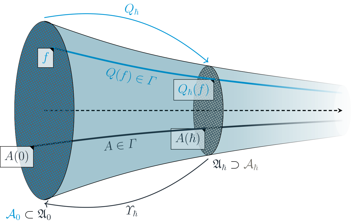
Figure 1: Continuous field of C*-algebras $(I,(\mathfrak{A}_{\hbar})_{\hbar\in I},\varGamma)$ with (continuous) sections $Q(f)$ (upper solid line, blue) and $A$ (lower solid line, black), a family of quantization maps $(Q_{\hbar})_{\hbar\in I}$ and dequantization maps $(\varUpsilon_{\hbar})_{\hbar\in I}$. At each value $\hbar\in I$ (horizontal axis), there is a quantum algebra $\mathfrak{A}_{\hbar}$ (ellipse, black) with a dense Poisson subalgebra $\mathcal{A}_{\hbar}$ (dotted patterns, blue/gray).

Furthermore, we want the quantization to admit a star product in the following sense.

Definition 5.

The quantization star product $\star_{Q}$ of a quantization — if it exists — is the star product (1) with operators $B_{Q,k}:\mathcal{A}_{0}\times\mathcal{A}_{0}\to\mathcal{A}_{0}$, such that for all $k\in\mathbb{N}$ and for all $f_{1},f_{2}\in\mathcal{A}_{0}$, the $k$-th order remainder

$$R_{Q}^{k}(f_{1},f_{2},\hbar) :=\frac{1}{\hbar^{k}}\left\|Q_{\hbar}(f_{1})Q_{\hbar}(f_{2})-\sum_{j=0}^{k}Q_{\hbar}\bigl{(}B_{Q,j}(f_{1},f_{2})\bigr{)}\hbar^{j}\right\|$$ (12)

vanishes in the classical limit,

$$\lim_{\hbar\to 0}R_{Q}^{k}(f_{1},f_{2},\hbar) =0.$$ (13)

Heuristically, the star product of two functions $f_{1}\star_{Q}f_{2}$ of an infinite order quantization $Q$ is an asymptotic expansion of $Q_{\hbar}^{-1}\bigl{(}Q_{\hbar}(f_{1})Q_{\hbar}(f_{2})\bigr{)}$, even though the inverse $Q_{\hbar}^{-1}$ usually does not exist even if the star product exists.

Definition 6.

A quantization $Q$ is an infinite order strict deformation quantization if

1. there exists a continuous field of C*-algebras $(I,(\mathfrak{A}_{\hbar})_{\hbar\in I},\varGamma)$ such that

   $$\forall f \in\mathcal{A}_{0}\subseteq\mathfrak{A}_{0}: Q(f) \in\varGamma,$$ (14)

2. the quantization star product $\star_{Q}$ exists, and

3. the star product is Poisson compatible.

We now consider sections that are well-behaved with respect to quantization and dequantization.

Definition 7.

A section $A\in\varGamma$ of the continuous field of C*-algebras $(I,(\mathfrak{A}_{\hbar})_{\hbar\in I},\varGamma)$ is $Q$-quantization expandable (quantization expandable or $Q$-expandable for short) if for any $k\in\mathbb{N}$

$$\exists f_{0},\dots,f_{k} \in\mathcal{A}_{0}: \lim_{\hbar\to 0}\frac{1}{\hbar^{k}}\left\|A(\hbar)-\sum_{j=0}^{k}Q_{\hbar}(f_{j})\hbar^{j}\right\| =0$$ (15)

and it is $\varUpsilon$-dequantization expandable (dequantization expandable or $\varUpsilon$-expandable for short) if for any $k\in\mathbb{N}$

$$\exists f_{0},\dots,f_{k} \in\mathcal{A}_{0}: \lim_{\hbar\to 0}\frac{1}{\hbar^{k}}\left\|\varUpsilon_{\hbar}(A(\hbar))-\sum_{j=0}^{k}f_{j}\hbar^{j}\right\| =0.$$ (16)

Denote the space of $\varUpsilon$-expandable sections by $\varGamma_{\varUpsilon}\subseteq\varGamma$ and let $\varSigma^{k}_{\varUpsilon}(\cdot,\hbar):\varGamma_{\varUpsilon}\to\mathcal{A}_{0}[[\hbar]]$ map to the expansion of any section $A\in\varGamma_{\varUpsilon}$ by the functions from (16) truncated at order $k$,

$$\varSigma^{k}_{\varUpsilon}(A,\hbar) :=\sum_{j=0}^{k}f_{j}\hbar^{j}.$$ (17)

On the one hand, it is immediately seen that the quantization section $Q(f)\subset\varGamma$ for any $f\in\mathcal{A}_{0}$ is $Q$-expandable with $f_{0}=f$ and $f_{k}=0$ for all $k>0$. On the other hand, if the space of $\varUpsilon$-expandable sections forms a *-subalgebra of $\varGamma$, then dequantization also admits a star product (which is not necessarily Poisson compatible).

Definition 8.

The dequantization star product $\star_{\varUpsilon}$ is the star product (1) with operators $B_{\varUpsilon,k}:\mathcal{A}_{0}\times\mathcal{A}_{0}\to\mathcal{A}_{0}$ such that for all $k\in\mathbb{N}$ and any dequantization expandable sections $A_{1},A_{2}\in\varGamma_{\varUpsilon}\subseteq\varGamma$, the expansion map intertwines $\star_{\varUpsilon}$ with the product on $\varGamma$, meaning

$$\varSigma^{k}_{\varUpsilon}(A_{1}A_{2},\hbar) =\sum_{j=0}^{k}B_{\varUpsilon,j}\bigl{(}\varSigma^{k}_{\varUpsilon}(A_{1},\hbar),\varSigma^{k}_{\varUpsilon}(A_{2},\hbar)\bigr{)}\hbar^{j}\mod\hbar^{k+1}.$$ (18)

Definition 9.

Given a continuous field of C*-algebras $(I,(\mathfrak{A}_{\hbar})_{\hbar\in I},\varGamma)$, a dequantization $\varUpsilon$ is an infinite order strict deformation dequantization if

1. the dequantization of any section $A\in\varGamma$,

   $$\varUpsilon(A):\mathcal{M}\times I \to\mathbb{C}, \varUpsilon(A)(x,\hbar) \mapsto\varUpsilon_{\hbar}(A(\hbar))(x),$$ (19)

   is a continuous function $\varUpsilon(A)\in\mathrm{C}(\mathcal{M}\times I,\mathbb{C})$,

2. the dequantization star product $\star_{\varUpsilon}$ exists, and

3. the star product is Poisson compatible.

The construction of a strict deformation quantization, a corresponding continuous field of C*-algebras $(I,(\mathfrak{A}_{\hbar})_{\hbar\in I},\varGamma)$ and a corresponding strict deformation dequantization can be quite complicated in the general case. We consider the case of a vector space in Section 4.

Given a symplectic manifold $(\mathcal{M},\omega)$ with a symplectic form $\omega$ that fulfills a certain integrality condition, there exists a quantization bundle over $\mathcal{M}$ and we can consider geometric quantization as below.

   Geometric Quantization

Definition 10.

Let $(\mathcal{M},\omega)$ be a real, symplectic manifold. For some $\hbar$, a quantization bundle is a Hermitian line bundle $\mathcal{L}_{\hbar}\to\mathcal{M}$ with connection $\nabla_{\hbar}$ that preserves the inner product, such that its curvature $R^{\mathcal{L}_{\hbar}}$ is proportional to the symplectic form,

$$R^{\mathcal{L}_{\hbar}}:=\left(\nabla_{\hbar}\right)^{2} =-\frac{\mathrm{i}}{\hbar}\omega.$$ (20)

Given a symplectic manifold, a quantization bundle does not necessarily exist and is not necessarily unique. A quantization bundle for $(\mathcal{M},\omega)$ exists if and only if the cohomology class of $\omega/2\text{p}\hbar$ in $H^{2}(\mathcal{M},\mathbb{R})$ is integral. This is known as the prequantization (or integrality) condition, see [2, Sec. 3].

For geometric quantization, it is furthermore necessary to find a “physical” Hilbert space $\mathcal{H}_{\hbar}$ as a subspace of the space of square-integrable sections $\mathrm{L}^{2}{}(\mathcal{M},\mathcal{L}_{\hbar})$ (or valued in $\mathcal{L}_{\hbar}$ tensored with some vector bundle). In some cases, the space $\mathcal{H}_{\hbar}$ is determined by a polarization [2].

Definition 11.

Let $(\mathcal{M},\omega)$ be an $2N$-dimensional real symplectic manifold and $\mathcal{L}_{\hbar}\to\mathcal{M}$ a quantization bundle. A (complex) polarization is a subbundle $P\subset(\mathrm{T}\mathcal{M})^{\mathbb{C}}$ that is involutive, $X,Y\in\varGamma(P)\implies[X,Y]\in\varGamma(P)$, and maximally isotropic (Lagrangian), $\forall X,Y\in\varGamma(P):\omega(X,Y)=0$ and $\forall x\in\mathcal{M}:\dim_{\mathbb{C}}P_{x}=N$. We say that a section $\psi\in\varGamma(\mathcal{M},\mathcal{L}_{\hbar})$ is polarized if $\forall X\in\varGamma(P):\nabla_{\hbar,X}\psi=0$. The physical Hilbert space $\mathcal{H}_{\hbar}$ is constructed from polarized sections of $\mathcal{L}_{\hbar}$.

For a Kähler manifold (a symplectic manifold with a compatible complex structure, $J$), the Kähler polarization is the subbundle on which $J$ has eigenvalue $-\mathrm{i}$, and the polarized sections are precisely the holomorphic sections. Compact Kähler manifolds have been studied before, see [6; 19; 30].

For the more general case of a symplectic manifold without pre-defined complex structure, we will consider an alternative construction of the physical Hilbert space from the spectrum of a Laplace operator in Subsection 2.5.

   (Berezin-)Toeplitz Quantization and Dequantization

For a given symplectic manifold $(\mathcal{M},\omega)$, suppose that a Hilbert subspace $\mathcal{H}_{\hbar}\subset\mathrm{L}^{2}{}(\mathcal{M},\mathcal{L}_{\hbar})$ has been constructed. Let

$$\varPi_{\hbar}:\mathrm{L}^{2}{}(\mathcal{M},\mathcal{L}_{\hbar}) \to\mathcal{H}_{\hbar}$$ (21)

be the projector to this Hilbert space. With the given Hilbert space $\mathcal{H}_{\hbar}$, we also obtain a quantization map [12].

Definition 12.

The (Berezin-)Toeplitz quantization map $T_{\hbar}$ assigns a bounded operator on the Hilbert space $\mathcal{H}_{\hbar}$ to every classical observable,

$$T_{\hbar}:\mathcal{A}_{0} \to\mathcal{B}(\mathcal{H}_{\hbar}),$$ (22)

using the projection $\varPi_{\hbar}$ from the space of square-integrable sections $\mathrm{L}^{2}{}(\mathcal{M},\mathcal{L}_{\hbar})$ such that

$$\forall\psi \in\mathcal{H}_{\hbar}: T_{\hbar}(f)\psi =\varPi_{\hbar}(f\psi).$$ (23)

For each $\hbar\in I$, we also choose an algebra $\mathfrak{A}_{\hbar}\subseteq\mathcal{B}(\mathcal{H}_{\hbar})$ such that it contains the image of $T_{\hbar}$. The Toeplitz quantization map $T_{\hbar}$ is linear and respects involution. Its domain actually extends to all bounded functions $\mathrm{C}_{\mathrm{b}}{}(\mathcal{M},\mathbb{C})$ so that $1\in\mathrm{C}_{\mathrm{b}}{}(\mathcal{M},\mathbb{C})$ is mapped to $\mathds{1}\in\mathcal{B}(\mathcal{H}_{\hbar})$. However, it will be easier to use the C*-algebra of compact operators $\mathfrak{A}_{\hbar}=\mathcal{K}(\mathcal{H}_{\hbar})$ in the construction of a continuous field of C*-algebras. Note that $\mathfrak{A}_{\hbar}$ coincides with $\mathcal{B}(\mathcal{H}_{\hbar})$ if $\dim\mathcal{H}_{\hbar}<\infty$. Furthermore, it will also be necessary to restrict to a dense subalgebra $\mathcal{A}_{0}\subset\mathfrak{A}_{0}$ for the construction of formal deformation quantizations (star products).

If the Toeplitz operators of compactly supported functions $\mathrm{C}_{\mathrm{c}}{}(\mathcal{M},\mathbb{C})$ on the physical Hilbert space $\mathcal{H}_{\hbar}$ are of trace-class, we define a measure $\mu_{\hbar}$ such that

$$\operatorname{Tr}(T_{\hbar}(f)) =\int\limits_{\mathcal{M}}f\;\mathrm{d}\!\!\;{}{\mu_{\hbar}}$$ (24)

holds for all $f\in\mathrm{C}_{\mathrm{c}}{}(\mathcal{M},\mathbb{C})$. When such a measure exists, we have an adjoint operation to Toeplitz quantization.

Definition 13.

Suppose the measure $\mu_{\hbar}$ determined by (24) exists. The (Berezin)-Toeplitz dequantization is a family of linear maps

$$\varXi_{\hbar}:\mathfrak{A}_{\hbar} \to\mathfrak{A}_{0},$$ (25)

such that for all complex-valued, compactly supported functions $f\in\mathrm{C}_{\mathrm{c}}{}(\mathcal{M},\mathbb{C})$ and all operators $A_{\hbar}\in\mathfrak{A}_{\hbar}$

$$\operatorname{Tr}(A_{\hbar}T_{\hbar}(f)) =\int\limits_{\mathcal{M}}\varXi_{\hbar}(A_{\hbar})f\;\mathrm{d}\!\!\;{}{\mu_{\hbar}}.$$ (26)

Consider the case of a symplectic manifold with a physical Hilbert space $\mathcal{H}_{\hbar}$ such that Toeplitz dequantization exists. If the algebras $\mathfrak{A}_{\hbar}$ are unital, then Toeplitz dequantization preserves the unit, $\varXi_{\hbar}(\mathds{1})=1$ since the measure is normalized,

$$\forall f \in\mathrm{C}_{\mathrm{c}}{}(\mathcal{M},\mathbb{C}): \int_{\mathcal{S}}\varXi_{\hbar}(\mathds{1})f\;\mathrm{d}\!\!\;{}{\mu_{\hbar}} =\int_{\mathcal{S}}f\;\mathrm{d}\!\!\;{}{\mu_{\hbar}}.$$ (27)

Applying dequantization to a Toeplitz operator $T_{\hbar}(f)$ yields a “smearing” of the original function.

Definition 14.

The Berezin transform of a classical observable $f\in\mathcal{A}_{0}$ over the symplectic manifold $(\mathcal{M},\omega)$ is the dequantization of its Toeplitz operator, $(\varXi_{\hbar}\circ T_{\hbar})(f)$.

A function $f\in\mathcal{A}_{0}$ is sometimes referred to as the contravariant or lower symbol of the Toeplitz operator $T_{\hbar}(f)$, while the Berezin transform $(\varXi_{\hbar}\circ T_{\hbar})(f)$ is also called the covariant or upper symbol of $T_{\hbar}(f)$ [3].

   Geometric Quantization on a Symplectic Manifold with a Riemannian Metric

Given a symplectic manifold with Riemannian metric, we want to identify the physical Hilbert space as a subspace of quantization bundle sections that correspond to the lowest part of the spectrum of the Laplacian defined with the metric.

Definition 15.

Let $(\mathcal{M},\omega,g)$ be a symplectic manifold with Riemannian metric, $\mathcal{L}_{\hbar}\to\mathcal{M}$ be a quantization bundle for some $\hbar\in I_{*}$. The Bochner Laplacian $\Delta_{\hbar}$ is an unbounded operator on sections $\varGamma(\mathcal{M},\mathcal{L}_{\hbar})$ determined by the connection $\nabla_{\hbar}$ and metric $g$,

$$\Delta_{\hbar} =\nabla_{\hbar}^{*}\nabla_{\hbar}.$$ (28)

In the case of a Kähler manifold, let $\nabla_{i}$ denote the holomorphic and $\nabla_{\bar{\jmath}}$ the anti-holomorphic components of the connection $\nabla_{\hbar}$, with $i\in[1,N]$, $\bar{\jmath}\in[\bar{1},\bar{N}]$. There is another, naturally defined Laplace operator, the Kodaira Laplacian

$$\Delta^{\mathrm{K}}_{\hbar} =-g^{i\bar{\jmath}}\nabla_{i}\nabla_{\bar{\jmath}}$$ (29)

using the summation convention. The Kodaira Laplacian is related to the Bochner Laplacian,

$$2\Delta^{\mathrm{K}}_{\hbar} =\Delta_{\hbar}-\frac{N}{\hbar}.$$ (30)

With the Kähler polarization, the physical Hilbert space is constructed from the space of holomorphically polarized sections with respect to the complex structure of the Kähler manifold. The kernel of the Kodaira Laplacian (29) contains the space of holomorphic sections. In fact, the kernel is precisely the space of holomorphic sections since the holomorphic components $\nabla_{i}$ are adjoint to the anti-holomorphic components $\nabla_{\bar{\imath}}$. We will show this for a symplectic vector space in Section 4. The Kodaira Laplacian is positive, so the space of holomorphic sections is the eigenspace of the Bochner Laplacian corresponding to the lowest eigenvalue $\frac{N}{\hbar}$, see (30). Thus, the physical Hilbert space is equivalently determined from the spectrum of the Bochner Laplacian.

In [15], it was shown how to use a renormalized Bochner Laplacian for a natural generalization to almost Kähler manifolds (with a non-integrable, almost complex structure). The renormalized Bochner Laplacian is a generalization of the expression on the right hand side of (30) and coincides with $2\Delta^{\mathrm{K}}_{\hbar}$ in the Kähler case, see also [7]. A choice of a physical Hilbert space is again given by the eigenspace corresponding to the lowest part of the spectrum, even though the lowest part does not have to be a single eigenvalue anymore.

A further generalization starts with a symplectic manifold with Riemannian metric but without pre-defined complex structure, see [23; 24]. For this, consider a $2N$-dimensional, compact, real, symplectic manifold $(\mathcal{M},\omega)$ with quantization bundle $\mathcal{L}_{\hbar}\to\mathcal{M}$ and Riemannian metric $g$. There exists an anti-self-adjoint linear map $E:\mathrm{T}\mathcal{M}\to\mathrm{T}\mathcal{M}$ such that for all $v_{1},v_{2}\in\mathrm{T}\mathcal{M}$

$$\omega(v_{1},v_{2}) =g(v_{1},E^{-1}v_{2}).$$ (31)

There exists an almost complex structure $J:\mathrm{T}\mathcal{M}\to\mathrm{T}\mathcal{M}$ such that $g(Jv_{1},Jv_{2})=g(v_{1},v_{2})$ and $\omega(Jv_{1},Jv_{2})=\omega(v_{1},v_{2})$ for all $v_{1},v_{2}\in\mathrm{T}\mathcal{M}$. We define a new metric $\eta$ such that for all $v_{1},v_{2}\in\mathrm{T}\mathcal{M}$

$$\eta(v_{1},v_{2}) :=\omega(v_{1},Jv_{2}).$$ (32)

The almost complex structure commutes with $E^{-1}$, so

$$J =-E^{-1}|E|.$$ (33)

At every point $x\in\mathcal{M}$, the operator $E^{-1}_{x}$ is an endomorphism and we denote half the trace of $|E_{x}|^{-1}$ as

$$\lambda(x) :=\frac{1}{2}\operatorname{tr}\bigl{(}J_{x}E^{-1}_{x}\bigr{)}=\frac{1}{2}\operatorname{tr}|E_{x}|^{-1}.$$ (34)

Note that in the special case of a Kähler manifold with a Kähler metric so that $E_{x}=\mathrm{id}$, this trace is $N$, half the real dimension of $\mathcal{M}$.

It was shown that the trace $\lambda(x)$ is positive for all $x\in\mathcal{M}$. A renormalized Bochner Laplacian $\Delta_{\hbar,\varPhi}$ is then defined with $\lambda$ and a smooth Hermitian section $\varPhi$ on a tensor product of the quantization line bundle with a vector bundle, see [22]. They have shown — using $\mathrm{Spin}^{\mathbb{C}}$ Dirac operators — that there exist two positive constants $\kappa$ and $\mu$ that are independent of $\hbar$, such that the spectrum of the renormalized Bochner Laplacian fulfills

$$\operatorname{spec}(\Delta_{\hbar,\varPhi}) \subset[-\kappa,\kappa]\cup\left[\frac{2\mu}{\hbar}-\kappa,\infty\right).$$ (35)

Given the spectrum condition (35) of the renormalized Bochner Laplacian on a symplectic manifold with Riemannian metric $(\mathcal{M},\omega,g)$ with quantization bundle $\mathcal{L}_{\hbar}\to\mathcal{M}$, the physical Hilbert space $\mathcal{H}_{\hbar}\subset\mathrm{L}^{2}{}(\mathcal{M},\mathcal{L}_{\hbar})$ is spanned by the sections corresponding to the lower part of the spectrum i.e., the part contained in $[-\kappa,\kappa]$.

For a symplectic vector space with inner product $(\mathcal{S},\omega,\left\langle\cdot,\;\!\cdot\right\rangle)$ as described in Section 3, we will use the idea of this construction to derive the physical Hilbert space $\mathcal{H}_{\hbar}$ in Section 4. The inner product gives the metric $g$ and we use a basis of holomorphic and anti-holomorphic vectors to express components with indices raised and lowered by $g$. This choice of a complex basis will allow us to write the sections of the Hilbert space as holomorphic sections with respect to the complex structure $J$ given by (33).

     Kähler Vector Space and the Sorkin-Johnston State

In this section, we introduce the symplectic vector space with an inner product that arises naturally in QFT on causal sets.

After the review of algebraic QFT on causal sets [9], we review the original construction of the Sorkin-Johnston state from a set of axioms [32].

   Scalar fields on causal sets

In the algebraic formulation of classical scalar fields on a (finite subset of a) causal set $\mathcal{C}$ as considered in [9], we start with the off-shell configuration space (a vector space) $\mathcal{E}$ of real-valued functions over $\mathcal{C}$ that is equipped with an inner product $\left\langle\cdot,\;\!\cdot\right\rangle$. We are interested in those real-valued functions over $\mathcal{C}$ that obey a discretized version of the Klein-Gordon field equations.

Given the Pauli-Jordan operator $E_{\mathrm{off}}\in\operatorname{End}(\mathcal{E})$ as the difference of the retarded and advanced Green’s operators for the field equations, the space of classical observables $\mathfrak{P}_{\mathrm{off}}$ is the space of complex-valued functions over the configuration space $\mathcal{E}$ with a Poisson structure $\pi_{\mathrm{off}}\in\bigwedge^{2}\mathcal{E}$ so that for all $f_{1},f_{2}\in\mathfrak{P}_{\mathrm{off}}$:

$${\left\{f_{1},\;\!f_{2}\right\}^{\mathrm{}}}_{\mathrm{off}}=\pi_{\mathrm{off}}(\mathrm{d}\!\!\;{}{f_{1}},\mathrm{d}\!\!\;{}{f_{2}}).$$ (36)

Note that this bracket is equivalently expressed as the map $\pi_{\mathrm{off}}^{\sharp}:\mathcal{E}^{*}\to\mathcal{E}$. In general, $\pi_{\mathrm{off}}^{\sharp}$ is degenerate but its image is an even dimensional sub-space $\mathcal{S}=\operatorname{img}(\pi_{\mathrm{off}}^{\sharp})\subset\mathcal{E}$. The on-shell Poisson algebra $\mathfrak{P}$ is then the quotient of $\mathfrak{P}_{\mathrm{off}}$ by the ideal generated by all observables that vanish on $\mathcal{S}$ [9]. We write the Poisson bracket on $\mathfrak{P}$ as $\left\{\cdot,\;\!\cdot\right\}^{\mathrm{}}$ and note that the corresponding map $\pi^{\sharp}:\mathcal{S}^{*}\to\mathcal{S}$ is now non-degenerate. The inner product on $\mathcal{E}$ restricts to an inner product $\left\langle\cdot,\;\!\cdot\right\rangle$ on $\mathcal{S}$ and determines the metric $g^{\flat}:\mathcal{S}\to\mathcal{S}^{*}$. The inverse of the Poisson bracket is a symplectic form $\omega$ on $\mathcal{S}$, which we express with the inverse of the (restricted) Pauli-Jordan operator $E\in\operatorname{End}(\mathcal{S})$,

$$\forall v_{1},v_{2} \in\mathcal{S}: \omega(v_{1},v_{2}) =\left\langle v_{1},\;\!E^{-1}v_{2}\right\rangle.$$ (37)

This structure on the vector space $\mathcal{S}$ is our starting point for the state construction. For a globally hyperbolic spacetime manifold, a symplectic vector space is similarly constructed from the configuration space of smooth functions. In that case, the symplectic vector space is infinite dimensional. However, our main focus in this work lies on the given structure for a finite dimensional vector space.

The operator $E$ is anti-symmetric and anti-self-adjoint, $E^{*}=-E$. As we have constructed a symplectic vector space, the kernel of the Pauli-Jordan operator $E$ (restricted to $\mathcal{S}$) is trivial and we have the polar decomposition

$$E =|E|U^{*},$$ (38a)

$$E^{*} =U|E|.$$ (38b)

where $U$ is a unitary operator and $|E|$ is the strictly positive operator i.e., invertible

$$|E| :=\sqrt{E^{*}E}=\sqrt{-E^{2}}.$$ (39)

We insert this decomposition into (37) to find

$$\forall v_{1},v_{2} \in\mathcal{S}: -\omega(v_{1},Uv_{2}) =\left\langle v_{1},\;\!|E|^{-1}v_{2}\right\rangle.$$ (40)

Since $|E|^{-1}$ is a positive, self-adjoint operator, the right hand side of (40) is also a symmetric, bi-linear form. We denote this form by $\eta$,

$$\forall v_{1},v_{2} \in\mathcal{S}: \eta(v_{1},v_{2}) :=\left\langle v_{1},\;\!|E|^{-1}v_{2}\right\rangle.$$ (41)

The operator $J=-U$ is a complex structure on $\mathcal{S}$ (such that $J^{2}=-\mathds{1}$) and the relation between $\omega$ and $\eta$ is Kähler.

Definition 16.

A Kähler vector space is a quadruple $(\mathcal{S},\omega,\eta,J)$ of a vector space $\mathcal{S}$ with a complex structure $J$, a symmetric bi-linear form $\eta$, and a symplectic form $\omega$ such that

$$\forall v_{1},v_{2} \in\mathcal{S}: \omega(v_{1},Jv_{2}) =\eta(v_{1},v_{2}).$$ (42)

Note that, on the one hand, in the presence of a complex structure $J$, the real vector space $\mathcal{S}$ turns into a complex vector space $\mathcal{S}_{J}$ by

$$\forall v\in\mathcal{S}:\forall a,b \in\mathbb{R}: (a+\mathrm{i}b)v :=av+bJv.$$ (43)

with $\dim_{\mathbb{C}}\mathcal{S}_{J}=\frac{1}{2}\dim_{\mathbb{R}}\mathcal{S}$. On the other hand, the complexification of $\mathcal{S}$ yields a complex vector space $\mathcal{S}^{\mathbb{C}}$ such that $\dim_{\mathbb{C}}\mathcal{S}^{\mathbb{C}}=\dim_{\mathbb{R}}\mathcal{S}$. The complexified vector space has a holomorphic $\mathcal{S}^{\mathbb{C},+}$ and an anti-holomorphic $\mathcal{S}^{\mathbb{C},-}$ subspace,

$$\mathcal{S}^{\mathbb{C},\pm} :=\left\{v\mp\mathrm{i}Jv\;\middle|\;v\in\mathcal{S}\right\}.$$ (44)

In the following, we use the complex vector space $\mathcal{S}_{J}$ (or equivalently the holomorphic subspace $\mathcal{S}^{\mathbb{C},+}$).

   The Sorkin-Johnston State

The main argument for the Sorkin-Johnston state [18; 31; 32] is that there exists a Hermitian operator

$$A_{\mathrm{SJ}} =\frac{1}{2}\bigl{(}|E|+\mathrm{i}E\bigr{)}$$ (45)

that yields the “positive eigenspace” of the operator $E$, and determines a two-point function [18]. We call $A_{\mathrm{SJ}}$ the Sorkin-Johnston operator on $\mathcal{S}_{J}$. By the one-to-one correspondence between two-point functions and quasi-free states, the bi-linear form $\eta$ determines the covariance of a quasi-free state.

Definition 17.

Let $\mathcal{W}_{\hbar}(\mathcal{S}^{*})$ be the Weyl algebra spanned by the Weyl generators $W_{\hbar}(\phi)$ (labelled by linear functionals $\phi\in\mathcal{S}^{*}=\operatorname{Hom}(\mathcal{S},\mathbb{R})$) as defined in Appendix A. The Sorkin-Johnston state $\sigma_{\mathrm{SJ}}:\mathcal{W}_{\hbar}(\mathcal{S}^{*})\to\mathbb{C}$ is the quasi-free (or Gaussian) state with a covariance given by the inverse of the symmetric, bi-linear form $\eta$ as defined in (41), so that for all $\phi\in\mathcal{S}^{*}$

$$\sigma_{\mathrm{SJ}}\bigl{(}W_{\hbar}(\phi)\bigr{)} =\exp\left(-\frac{\hbar}{4}\eta^{-1}(\phi,\phi)\right).$$ (46)

More generally, for a quasi-free state with covariance $\gamma$, the bi-linear form $\eta_{\mathrm{G}}=\gamma^{-1}$ and the symplectic form $\omega$ satisfy the Cauchy-Schwarz inequality, $\forall v_{1},v_{2}\in\mathcal{S}$:

$$\left|\omega(v_{1},v_{2})\right|^{2} \leq\eta_{\mathrm{G}}(v_{1},v_{1})\eta_{\mathrm{G}}(v_{2},v_{2}),$$ (47)

known as the domination condition [13].

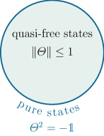
Figure 2: Operator norm of the operator $\varTheta$ determined by the symplectic form and the inner product $\eta_{\mathrm{G}}$ as given in (48). For pure states, the operator norm lies on the boundary of this graphical representation and $\varTheta$ is a complex structure.

Given a relation between the bi-linear forms $\omega$ and $\eta_{\mathrm{G}}$ such that for all $v_{1},v_{2}\in\mathcal{S}$:

$$\omega(v_{1},\varTheta v_{2}) =\eta_{\mathrm{G}}(v_{1},v_{2}),$$ (48)

the domination condition implies that $\|\varTheta\|\leq 1$. Figure 2 illustrates this condition on the operator norm, where the norm is induced by the inner product. For the proofs of the equivalences of the three statements, see [8].

For the structure that determines the Sorkin-Johnston state, the operator $\varTheta=J$ is a complex structure, meaning that $\varTheta^{2}=-\mathds{1}$, so that $\|\varTheta\|=1$ and (47) is saturated. This means that the Sorkin-Johnston state is pure – it cannot be written as a convex combination of two other states. By the one-to-one correspondence between quasi-free states and two-point functions, the Sorkin-Johnston state corresponds to a two-point function determined by the Sorkin-Johnston operator $A_{\mathrm{SJ}}$.

   The Sorkin-Johnston Axioms

Sorkin and Johnston formulated the described properties that yield the unique quasi-free state (46) as a set of axioms. In our notation, these axioms are conditions for the Sorkin-Johnston operator $A_{\mathrm{SJ}}$ and its (element-wise) complex conjugate $\overline{A}_{\mathrm{SJ}}$ acting on the complexified vector space $\mathcal{S}^{\mathbb{C}}$. The Pauli-Jordan operator $E$ is extended to $\mathcal{S}^{\mathbb{C}}$.

Positivity: $$A_{\mathrm{SJ}} \geq 0,\allowdisplaybreaks[3]$$ (49a)

Commutator: $$A_{\mathrm{SJ}}-\overline{A}_{\mathrm{SJ}} =\mathrm{i}E,\allowdisplaybreaks[3]$$ (49b)

Purity: $$A_{\mathrm{SJ}}\overline{A}_{\mathrm{SJ}} =0.$$ (49c)

In order to solve these axioms, we introduce the operator

$$H :=2A_{\mathrm{SJ}}-\mathrm{i}E$$ (50)

and recall that $E$ is real by definition, $\overline{E}=E$. The positivity axiom implies that $H$ is positive semi-definite such that for all $v\in\mathcal{S}^{\mathbb{C}}$

$$0\leq\left\langle v,\;\!Hv\right\rangle+\mathrm{i}\left\langle v,\;\!Ev\right\rangle =\left\langle v,\;\!Hv\right\rangle,$$ (51a)

Second, the commutator axiom states that the operator $$H$$ is real (has real components). So, the third axiom splits into real and imaginary parts,

$$H^{2}+E^{2} =0,\allowdisplaybreaks[3]$$ (51b)

$$EH-HE =0.$$ (51c)

Since $E$ is non-degenerate, use the polar decomposition (38) to find that (51b) gives $H=\pm|E|$. With the positivity axiom, there is only one solution

$$H =|E|.$$ (52)

In summary, the full unique solution for the Sorkin-Johnston operator reads

$$A_{\mathrm{SJ}} =\frac{1}{2}\bigl{(}|E|+\mathrm{i}E\bigr{)}.$$ (53)

This operator is self-adjoint and it determines a two-point function [18; 32].

In this motivating discussion, we reviewed the Sorkin-Johnston axioms that describe a pure, quasi-free state, corresponding to a complex structure $J$ on the vector space $\mathcal{S}$. We will start from the given structure of the symplectic form $\omega$ and the inner product $\left\langle\cdot,\;\!\cdot\right\rangle$ as symmetric bi-linear form over $\mathcal{S}$ to construct a quantum algebra by geometric quantization. Our construction will yield the Sorkin-Johnston state without imposing the Sorkin-Johnston axioms. Throughout the construction, the quantization parameter $\hbar$ is kept explicit to eventually define a field of algebras over all $\hbar\in I$ and discuss the classical limit.

     Quantization and Dequantization for a Symplectic Vector Space with Inner Product

Recall from Section 3 that, in our case, we have a $2N$-dimensional real, symplectic vector space with an inner product $(\mathcal{S},\omega,\left\langle\cdot,\;\!\cdot\right\rangle)$ and a non-degenerate operator $E$ relating the symplectic form to the inner product given by (37).

   Geometric Quantization and the Laplacian

We showed the general idea of geometric quantization in Section 2. For the vector space, $\mathcal{S}$, we want to construct the physical Hilbert space $\mathcal{H}_{\hbar}$ as a subspace of square integrable sections $\mathrm{L}^{2}{}(\mathcal{S},\mathcal{L}_{\hbar})$ on the quantization bundle $\mathcal{L}_{\hbar}\to\mathcal{S}$. We will derive the spectrum of the Bochner Laplacian (28) and then define the Hilbert space $\mathcal{H}_{\hbar}$ from the sections corresponding to the lowest part of the spectrum — which will turn out to be a single eigenvalue as in the Kähler case. For the derivation, we will use the operator $\overline{\mathcal{D}}$ induced by the complex structure $J$ that is derived from the symplectic form $\omega$ and the metric $g$ (corresponding to the inner product $\left\langle\cdot,\;\!\cdot\right\rangle$), see (33). The complex structure will serve merely as a tool in the derivation of the spectrum so that it becomes obvious that the Hilbert space (corresponding to the lowest spectral value of the Laplacian) is the space of holomorphic sections. At some points in the derivation, we will write the elements of $\mathcal{S}$ in complex coordinates $z_{i},\bar{z}_{\bar{\imath}}$ where we denote the holomorphic indices by $i\in[1,N]$ and the anti-holomorphic indices by $\bar{\imath}\in[\bar{1},\bar{N}]$ corresponding to the derived complex structure (33). However, the result of the spectrum will not depend on the choice of coordinates. We are defining the physical Hilbert space from the spectrum of the Laplacian, which will turn out to be equivalent to the holomorphic sections with respect to a complex structure $J$ that is compatible with the symplectic form $\omega$ and the derived metric $\eta$.

Consider an exact symplectic form $\omega=-\mathrm{d}\!\!\;{}\theta$, a trivial line bundle $\mathcal{L}_{\hbar}=\mathcal{S}\times\mathbb{C}$, and the non-trivial connection parametrized by $\hbar$,

$$\nabla_{\hbar} =\mathrm{d}\!\!\;{}+\frac{\mathrm{i}}{\hbar}\theta.$$ (54)

With the complex structure $J$ given as in (33), we turn the real vector space $\mathcal{S}$ into a complex vector space $\mathcal{S}_{J}$ by the assignment (43). The operator $\nabla_{\hbar}$ increases the total degree $p+q$ of complex differential forms $\varOmega^{p,q}$ by 1. We define operators $\mathcal{D}^{+}_{\hbar}:\varOmega^{p,q}\to\varOmega^{p+1,q}$ raising the holomorphic degree and $\overline{\mathcal{D}}{}^{+}_{\hbar}:\varOmega^{p,q}\to\varOmega^{p,q+1}$ raising the anti-holomorphic degree such that

$$\nabla_{\hbar} =\mathcal{D}^{+}_{\hbar}+\overline{\mathcal{D}}{}^{+}_{\hbar}.$$ (55)

Use the Hodge dual operator ${\ast}:\varOmega^{p,q}\to\varOmega^{N-q,N-p}$ to define an inner product for square-integrable sections $\psi,\phi\in\varOmega^{p,q}$

$$\left\langle\psi,\;\!\phi\right\rangle_{\varOmega}:=\int\limits_{\mathcal{S}}\overline{\psi}\wedge{\ast}\phi.$$ (56)

Cauchy complete the space of square-integrable sections (such that the inner product (56) is finite) to a Hilbert space. The respective adjoint operators of the split in (55) are

$$\mathcal{D}^{-}_{\hbar} :=-{\ast}\overline{\mathcal{D}}{}^{+}_{\hbar}{\ast},\allowdisplaybreaks[3]$$ (57a)

$$\overline{\mathcal{D}}{}^{-}_{\hbar} :=-{\ast}\mathcal{D}^{+}_{\hbar}{\ast}.$$ (57b)

We illustrate the domains and codomains of the complex differential operators in Figure 3.

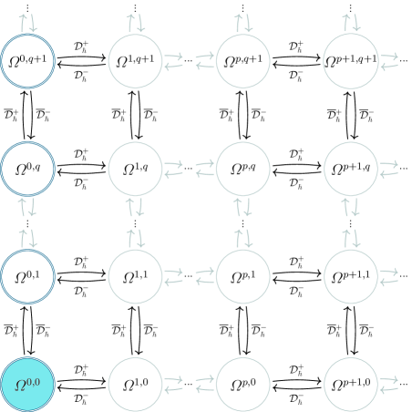
Figure 3: Complex differential operators mapping between the spaces of differential forms valued in $\mathcal{L}_{\hbar}$. For the derivation of the spectrum, our attention lies on the $(0,0)$-forms and anti-holomorphic forms as shown on the left. Note that $\mathcal{D}^{-}_{\hbar}\varOmega^{0,q}=0$ and $\overline{\mathcal{D}}{}^{-}_{\hbar}\varOmega^{p,0}=0$.

In this work, our main focus lies on the forms with $p=q=0$ i.e., the sections of the line bundle $\psi\in\varOmega^{0,0}$ (marked in blue), so that the operators $\mathcal{D}^{-}_{\hbar}$ and $\overline{\mathcal{D}}{}^{-}_{\hbar}$ annihilate them, $\mathcal{D}^{-}_{\hbar}\psi=0,\overline{\mathcal{D}}{}^{-}_{\hbar}\psi=0$, so that they are not shown in Figure 3.

The Bochner Laplacian derived from the connection (55) and its Hodge dual (57) is

$$\Delta_{\hbar} =\mathcal{D}^{-}_{\hbar}\mathcal{D}^{+}_{\hbar}+\mathcal{D}^{-}_{\hbar}\overline{\mathcal{D}}{}^{+}_{\hbar}+\overline{\mathcal{D}}{}^{-}_{\hbar}\mathcal{D}^{+}_{\hbar}+\overline{\mathcal{D}}{}^{-}_{\hbar}\overline{\mathcal{D}}{}^{+}_{\hbar}.$$ (58)

As we show in Figure 3, for sections of the quantization bundle $\mathcal{L}_{\hbar}$, i.e. $(0,0)$-forms, only the left-most and right-most summand remain, because $\mathcal{D}^{-}_{\hbar}\varOmega^{0,0}=0$ and $\overline{\mathcal{D}}{}^{-}_{\hbar}\varOmega^{0,0}=0$.

For the following computation, we choose complex coordinates $z^{i}=x^{i}+\mathrm{i}y^{i}$ (with indices $i\in[1,N]$, $\bar{\imath}\in[\bar{1},\bar{N}]$) in which $|E|^{-1}$ is diagonal with diagonal components $\vartheta_{i}$. The computations for any $(p,q)$-forms using these coordinates are given in Appendix B. The indices are raised with the inverse metric $g^{\bar{\imath}i}$ derived from the inner product on $\mathcal{S}$. Raising an index also changes it from holomorphic to anti-holomorphic and vice versa. For a slightly compacter notation, we omit the $\hbar$ subscript whenever the connection $\nabla_{\hbar}$ is expressed in coordinates.

Following the results in Appendix B, express the difference of the first and last operator pair in (58) as contraction of the quantization bundle curvature,

$$\mathcal{D}^{-}_{\hbar}\mathcal{D}^{+}_{\hbar}-\overline{\mathcal{D}}{}^{-}_{\hbar}\overline{\mathcal{D}}{}^{+}_{\hbar} =g^{\bar{\imath}j}\left[\nabla_{j},\;\!\nabla_{\bar{\imath}}\right]_{-}\allowdisplaybreaks[3]$$ (59a)

$$=-\frac{\mathrm{i}}{\hbar}g^{\bar{\imath}j}\omega_{j\bar{\imath}}=:\lambda_{\hbar}.$$ (59b)

We use this identity to replace the first operator pair of the Bochner Laplacian (28) by the anti-holomorphic operators $\overline{\mathcal{D}}{}^{\pm}_{\hbar}$ along with the positive shift constant $\lambda_{\hbar}$, such that we obtain for $(0,0)$-forms

$$\Delta_{\hbar} =2\overline{\mathcal{D}}{}^{-}_{\hbar}\overline{\mathcal{D}}{}^{+}_{\hbar}+\lambda_{\hbar}\mathds{1}.$$ (60)

The constant $\lambda_{\hbar}$ is (up to the quantization parameter $\hbar$) half the trace of $|E|^{-1}$,

$$\lambda_{\hbar} =\frac{1}{2\hbar}\operatorname{tr}|E|^{-1}.$$ (61)

In our choice of complex coordinates such that $|E|^{-1}$ is diagonal, this constant is half the sum over all the diagonal components divided by $\hbar$.

Combine the operators $\overline{\mathcal{D}}{}^{\pm}_{\hbar}:\varOmega^{0,q}\to\varOmega^{0,q\pm 1}$ that increase and decrease the anti-holomorphic degree to a self-adjoint operator,

$$\overline{\mathcal{D}}_{\hbar} :=\overline{\mathcal{D}}{}^{+}_{\hbar}+\overline{\mathcal{D}}{}^{-}_{\hbar}.$$ (62)

So the Laplacian acting on $(0,0)$-forms $\psi\in\varOmega^{0,0}$ becomes

$$\Delta_{\hbar}\psi =2\overline{\mathcal{D}}_{\hbar}^{2}\psi+\lambda_{\hbar}\psi.$$ (63)

Since by construction the Laplacian and the operator $\overline{\mathcal{D}}_{\hbar}^{2}$ are self-adjoint and positive, $\lambda_{\hbar}$ is the lower bound on the spectrum of the Laplacian. We want to derive the spectrum of the Laplacian operator (related to the spectrum of $\overline{\mathcal{D}}_{\hbar}^{2}$) to identify the lowest eigenvalue and the corresponding space of lowest eigen-sections. This space is the physical Hilbert space for which we can construct an algebra of quantum observables.

In the following section, we derive the spectra of $\overline{\mathcal{D}}_{\hbar}^{2}$ (the operator sequence is shown in Figure 3 on the left) and the Laplacian. We can then use the space spanned by the lowest eigen-sections of the Laplacian as the physical Hilbert space for the construction of the quantum algebra.

For reference, the spectrum of an operator on a Hilbert space is defined in Appendix A. Starting with the spectrum of $\overline{\mathcal{D}}_{\hbar}^{2}$, let $\varOmega^{0,*}$ denote the space of sections of the powers of the anti-holomorphic cotangent bundle i.e., $(0,q)$-forms for any $q$. Let $\mathfrak{H}_{\hbar}^{0,\pm}$ be the Hilbert spaces of $(0,q)$-forms with even ($+$) or odd value ($-$) for the degree $q$. The operators $\overline{\mathcal{D}}{}^{\pm}_{\hbar}$ map between these Hilbert spaces as adjoint operators to each other.

   Spectral Gap of the Laplacian

In order to derive the spectrum, we make use of the decomposition of the symmetric bi-linear form into $N$ components. The operator $\overline{\mathcal{D}}_{\hbar}^{2}$ acts on sections of the quantization line bundle $\mathcal{L}_{\hbar}$ as

$$\overline{\mathcal{D}}_{\hbar}^{2} =\overline{\mathcal{D}}{}^{-}_{\hbar}\overline{\mathcal{D}}{}^{+}_{\hbar}=-g^{i\bar{\jmath}}\nabla_{i}\nabla_{\bar{\jmath}},$$ (64)

which is composed of holomorphic ($\nabla_{i}$) and anti-holomorphic ($\nabla_{\bar{\jmath}}$) derivative components of the covariant derivative, using the summation convention. The operator in (64) is the square of a self-adjoint operator and thus has a real, positive spectrum. We express the components of the symmetric bi-linear form $g^{i\bar{\jmath}}$ (corresponding to the inner product $\left\langle\cdot,\;\!\cdot\right\rangle$) in terms of the diagonal components $\vartheta_{i}$ of $|E|^{-1}$,

$$\bigl{(}g_{i\bar{\jmath}}\bigr{)}_{i\in[1,N],\bar{\jmath}\in[\bar{1},\bar{N}]} =\operatorname{diag}\Bigl{(}\frac{1}{\vartheta_{1}},\frac{1}{\vartheta_{2}},\dotso,\frac{1}{\vartheta_{N}}\Bigr{)},\allowdisplaybreaks[3]$$ (65a)

$$\bigl{(}g^{i\bar{\jmath}}\bigr{)}_{i\in[1,N],\bar{\jmath}\in[\bar{1},\bar{N}]} =\operatorname{diag}\bigl{(}\vartheta_{1},\vartheta_{2},\dotso,\vartheta_{N}\bigr{)}.$$ (65b)

Now, we decompose the operator $\overline{\mathcal{D}}_{\hbar}^{2}$ into a sum over operators $A^{\bar{\imath}}$ and $B^{i}$ such that

$$\overline{\mathcal{D}}_{\hbar}^{2} =(-\nabla_{i})(g^{i\bar{\jmath}}\nabla_{\bar{\jmath}})=:(\text{d}_{i\bar{\imath}}A^{\bar{\imath}})(B^{i}).$$ (66)

The components of the covariant derivative fulfill the commutation relations

$$\left[\nabla_{i},\;\!\nabla_{j}\right]_{-} =0,\allowdisplaybreaks[3]$$ (67a)

$$\left[\nabla_{i},\;\!\nabla_{\bar{\jmath}}\right]_{-} =-\frac{\mathrm{i}}{\hbar}\omega_{i\bar{\jmath}}=\frac{1}{\hbar}\text{d}_{i\bar{\jmath}},\allowdisplaybreaks[3]$$ (67b)

$$\left[\nabla_{\bar{\imath}},\;\!\nabla_{\bar{\jmath}}\right]_{-} =0.$$ (67c)

Thus commuting the operators $A^{\bar{\imath}}$ and $B^{i}$ gives

$$B^{i}A^{\bar{\imath}} =A^{\bar{\imath}}B^{i}+\frac{1}{\hbar}g^{i\bar{\imath}}.$$ (68)

Since both operator orders $B^{i}A^{\bar{\imath}}$ and $A^{\bar{\imath}}B^{i}$ are positive operators the spectrum of $B^{i}A^{\bar{\imath}}$ has the lower bound $g^{i\bar{\imath}}/\hbar$. With the help of the following lemma, the lower bound implies a spectral gap for $A^{\bar{\imath}}B^{i}$.

Lemma 18.

Let $A:\mathfrak{H}_{1}\to\mathfrak{H}_{2}$ and $B:\mathfrak{H}_{2}\to\mathfrak{H}_{1}$ be operators between Hilbert spaces $\mathfrak{H}_{1}$ and $\mathfrak{H}_{2}$; then

$$\{0\}\cup\operatorname{spec}(AB) =\{0\}\cup\operatorname{spec}(BA).$$ (69)

Proof.

To get the idea of the proof, first consider a pair of bounded operators $A\in\mathcal{B}(\mathfrak{H}_{1},\mathfrak{H}_{2})$ and $B\in\mathcal{B}(\mathfrak{H}_{2},\mathfrak{H}_{1})$ between two Hilbert spaces. For every $\lambda\in\operatorname{resol}(AB)\setminus\{0\}$ that is above the operator bound, $|\lambda|>\|AB\|$, there is a Neumann series

$$R =\frac{1}{\lambda}\left(\mathds{1}+\sum_{n=1}^{\infty}\left(\frac{AB}{\lambda}\right)^{n}\right),$$ (70)

which converges in norm. It is the inverse of $(\lambda\mathds{1}-AB)$,

$$(\lambda\mathds{1}-AB)R=\mathds{1}+\sum_{n=1}^{\infty}\left(\frac{AB}{\lambda}\right)^{n}-\frac{AB}{\lambda}-\sum_{n=2}^{\infty}\left(\frac{AB}{\lambda}\right)^{n} =\mathds{1}.$$ (71)

For the bounded operators, the series

$$\sum_{n=1}^{\infty}\left(\frac{BA}{\lambda}\right)^{n} =\frac{1}{\lambda}B\left(\sum_{n=1}^{\infty}\left(\frac{AB}{\lambda}\right)^{n-1}\right)A=\frac{1}{\lambda}BRA$$ (72)

is also well-defined. But the right hand side of equation (72), which does not include a summation anymore, can also be calculated for any resolvent $R$, where $\lambda\neq 0$. Thus we conclude the lemma with the proof for any (unbounded) operator pair $A$ and $B$ as follows.

Let $\lambda\in\operatorname{resol}(AB)\setminus\{0\}$ be any element not in the spectrum and not zero. Let $R$ be the resolvent for $\lambda$ and define

$$\tilde{R} :=\frac{1}{\lambda}\left(\mathds{1}+BRA\right).$$ (73)

Because $R$ exists, so does $\tilde{R}$. The multiplication with $(\lambda\mathds{1}-BA)$ from the left yields

$$(\lambda\mathds{1}-BA)\tilde{R} =\mathds{1}-\frac{1}{\lambda}BA+BRA-\frac{1}{\lambda}BABRA\allowdisplaybreaks[3]$$ (74a)

$$=\mathds{1}-\frac{1}{\lambda}BA+B\frac{1}{\lambda}(\lambda\mathds{1}-AB)RA\allowdisplaybreaks[3]$$ (74b)

$$=\mathds{1}$$ (74c)

and a multiplication from the right is shown similarly. This verifies that $\tilde{R}$ is a resolvent of $BA$, therefore $\lambda\in\operatorname{resol}(BA)$. Considering all $\lambda\in\operatorname{resol}(AB)\setminus\{0\}$, it follows that

$$\operatorname{resol}(AB)\setminus\{0\} \subset\operatorname{resol}(BA).$$ (75)

Repeating this procedure for the operator order $BA$, we also obtain

$$\operatorname{resol}(BA)\setminus\{0\} \subset\operatorname{resol}(AB).$$ (76)

Removing the zero element on the right hand sides of equations (75) and (76), we obtain

$$\operatorname{resol}(AB)\setminus\{0\} =\operatorname{resol}(BA)\setminus\{0\}.$$ (77)

Because the spectrum is the complement of the resolvent set, equation (77) implies that the union of the spectra with zero are identical too. ∎

We apply this lemma to the operator pair $A^{\bar{\imath}}B^{i}$ to prove that its spectrum has a gap.

Lemma 19.

The positive, self-adjoint operator pair $A^{\bar{\imath}}B^{i}$ (with $A^{\bar{\imath}}:\mathfrak{H}_{\hbar}^{0,\pm}\to\mathfrak{H}_{\hbar}^{0,\mp}$ and $B^{i}:\mathfrak{H}_{\hbar}^{0,\mp}\to\mathfrak{H}_{\hbar}^{0,\pm}$) that fulfills the commutation relation (68):

$$B^{i}A^{\bar{\imath}} =A^{\bar{\imath}}B^{i}+\frac{1}{\hbar}g^{i\bar{\imath}},$$

has a spectral gap between the spectral values $0$ and $\vartheta_{i}/\hbar$.

Proof.

Since the operator pairs $A^{\bar{\imath}}B^{i}$ and $B^{i}A^{\bar{\imath}}$ are positive and self-adjoint, we know that

$$\operatorname{spec}(A^{\bar{\imath}}B^{i}) \subset\left[0,\infty\right),\allowdisplaybreaks[3]$$ (78a)

$$\operatorname{spec}(B^{i}A^{\bar{\imath}}) \subset\left[0,\infty\right).$$ (78b)

Because $B^{i}=g^{i\bar{\jmath}}\nabla_{\bar{\jmath}}$, so that $0\in\operatorname{spec}(B^{i})$ and thus $0\in\operatorname{spec}(A^{\bar{\imath}}B^{i})$ with any holomorphic section as eigen-section i.e., the sections $\psi$ that fulfill

$$\nabla_{\bar{\imath}}\psi=\left(\frac{\partial}{{\partial{\overline{z}^{\bar{\imath}}}}}+\frac{\mathrm{i}}{\hbar}\theta_{\bar{\imath}}\right)\psi =0$$ (79)

in complex coordinates $z^{i},\bar{z}^{\bar{\imath}}$.

The spectral values of the operator pair $B^{i}A^{\bar{\imath}}$ are identical to those of $A^{\bar{\imath}}B^{i}$ up to the constant term given in (68), so that

$$0\in\operatorname{spec}(A^{\bar{\imath}}B^{i}) \Rightarrow\min\bigl{(}\operatorname{spec}(B^{i}A^{\bar{\imath}})\bigr{)}=\frac{\vartheta_{i}}{\hbar}.$$ (80)

After applying Lemma 18, we can summarize

$$\left\{0,\frac{1}{\hbar}g^{i\bar{\imath}}\right\} \subset\operatorname{spec}(A^{\bar{\imath}}B^{i}),\allowdisplaybreaks[3]$$ (81a)

$$\left(0,\frac{1}{\hbar}g^{i\bar{\imath}}\right) \not\subset\operatorname{spec}(A^{\bar{\imath}}B^{i}).$$ (81b)

So the only spectral value of $A^{\bar{\imath}}B^{i}$ smaller than $g^{i\bar{\imath}}/\hbar$ is 0. ∎

We choose a gauge for the symplectic potential such that

$$\theta =\frac{\mathrm{i}}{2}\text{d}_{i\bar{\jmath}}\left(\overline{z}^{\bar{\jmath}}\mathrm{d}\!\!\;{}{z^{i}}-z^{i}\mathrm{d}\!\!\;{}{\overline{z}^{\bar{\jmath}}}\right),$$ (82)

and we write

$$|z|^{2} =\text{d}_{i\bar{\imath}}z^{i}\overline{z}^{\bar{\imath}}.$$ (83)

In this gauge, any holomorphic section $\psi$ — as solutions to (79) — has an arbitrary, smooth, holomorphic function $\alpha$ as amplitude, so that for all $z\in\mathcal{S}$

$$\psi(z) =\frac{\alpha(z)}{\sqrt{2\text{p}\hbar}^{N}}\exp\left(-\frac{1}{2\hbar}|z|^{2}\right).$$ (84)

We repeat the application of the these lemmas to determine the spectrum of the Laplacian, so that we obtain the space of holomorphic sections (84) as the physical Hilbert space.

   Full Spectrum of the Laplacian

Any holomorphic section $\psi\in\varOmega^{0,0}$, as given in (84), is also a solution of the differential equation

$$\overline{\mathcal{D}}{}^{-}_{\hbar}\overline{\mathcal{D}}{}^{+}_{\hbar}\psi=-g^{i\bar{\jmath}}\nabla_{i}\nabla_{\bar{\jmath}}\psi =0.$$ (85)

This follows from the fact that $\overline{\mathcal{D}}{}^{-}_{\hbar}$ is the adjoint to $\overline{\mathcal{D}}{}^{+}_{\hbar}$ and thus

$$\left\langle\psi,\;\!\overline{\mathcal{D}}{}^{-}_{\hbar}\overline{\mathcal{D}}{}^{+}_{\hbar}\psi\right\rangle_{\varOmega} =\left\langle\overline{\mathcal{D}}{}^{+}_{\hbar}\psi,\;\!\overline{\mathcal{D}}{}^{+}_{\hbar}\psi\right\rangle_{\varOmega}$$ (86)

implies that $\overline{\mathcal{D}}{}^{+}_{\hbar}\psi$ has to vanish whenever $\overline{\mathcal{D}}{}^{-}_{\hbar}\overline{\mathcal{D}}{}^{+}_{\hbar}\psi$ does. Due to the diagonal form, all components $\nabla_{\bar{\jmath}}\psi$ have to vanish. Consequently, the eigenspace of $\Delta_{\hbar}$ for the eigenvalue (61),

$$\Delta_{\hbar}\psi =\lambda_{\hbar}\psi,$$ (87)

is spanned by the holomorphic sections (84). The following theorem then concludes our derivation of the spectrum.

Theorem 20.

Let $\Delta_{\hbar}$ be the Bochner Laplacian for sections of the quantization bundle $\mathcal{L}_{\hbar}\to\mathcal{S}$ over a real $2N$-dimensional symplectic vector space $(\mathcal{S},\omega,\left\langle\cdot,\;\!\cdot\right\rangle)$ with a non-degenerate symplectic form $\omega$ and an inner product $\left\langle\cdot,\;\!\cdot\right\rangle$. Let $\vartheta_{i}$ be the diagonal components as given in (65). The spectrum of the Laplacian is given by

$$\operatorname{spec}(\Delta_{\hbar}) =\left\{\frac{1}{\hbar}\sum_{i=1}^{N}(2n_{i}+1)\vartheta_{i}\;\middle|\;n_{i}\in\mathbb{N}\right\}.$$ (88)

Proof.

We have determined the spectral shift in (68):

$$\operatorname{spec}(B^{i}A^{\bar{\imath}}) =\operatorname{spec}(A^{\bar{\imath}}B^{i})+\frac{1}{\hbar}g^{i\bar{\imath}}.$$

Applying Lemma 18 to the spectral gap shown in Lemma 18 yields a secondary spectral gap,

$$\left\{\frac{1}{\hbar}g^{i\bar{\imath}},\frac{2}{\hbar}g^{i\bar{\imath}}\right\} \subset\operatorname{spec}(B^{i}A^{\bar{\imath}}),\allowdisplaybreaks[3]$$ (89a)

$$\left(\frac{1}{\hbar}g^{i\bar{\imath}},\frac{2}{\hbar}g^{i\bar{\imath}}\right) \not\subset\operatorname{spec}(B^{i}A^{\bar{\imath}}).$$ (89b)

An iteratively repeated application of Lemma 18 then yields the discrete spectra

$$\operatorname{spec}(B^{i}A^{\bar{\imath}}) =\frac{1}{\hbar}g^{i\bar{\imath}}\mathbb{N}_{*},\allowdisplaybreaks[3]$$ (90a)

$$\operatorname{spec}(A^{\bar{\imath}}B^{i}) =\frac{1}{\hbar}g^{i\bar{\imath}}\mathbb{N},$$ (90b)

where only the latter one includes zero.

Recombining the operators for all the $N$ components as defined in (65) and (66) gives

$$\operatorname{spec}\bigl{(}\overline{\mathcal{D}}{}^{-}_{\hbar}\overline{\mathcal{D}}{}^{+}_{\hbar}\bigr{)} =\sum_{i=1}^{N}\frac{\vartheta_{i}}{\hbar}\mathbb{N}$$ (91)

such that (88) follows by a scaling with 2 and shifting by $\lambda_{\hbar}$ according to (60). ∎

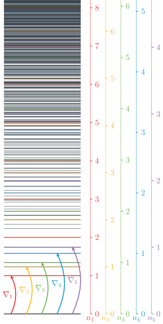
Figure 4: Illustration of the spectrum of the Bochner Laplacian $\Delta_{\hbar}=\nabla_{\hbar}^{*}\nabla_{\hbar}$ obtained with the holomorphic components of the covariant derivative $\nabla_{i}$ for five dimensions ($N=5$) weighted by distinct scaling factors $\vartheta_{i}$. All dark lines represent a value in the spectrum of the Laplacian, while the five colours highlight the levels reached by powers of the respective derivative components only. The lowest level (black) is the solution (84).

Figure 4 depicts the spectrum, which gets denser towards infinity. Note that the spectrum (88) does not depend on the complex structure $J$. We use the space of eigen-sections at the lowest spectral value as the physical Hilbert space $\mathcal{H}_{\hbar}$ on which bounded operators act as quantized observables. The complex structure $J$ is determined by the operator $E^{-1}$ in (33) such that the eigenspace of the lowest spectral value corresponds to the holomorphic sections (84).

   The Physical Hilbert Space

Following the general construction from Subsection 2.5, we define the physical Hilbert space $\mathcal{H}_{\hbar}\subset\mathrm{L}^{2}{}(\mathcal{S},\mathcal{L}_{\hbar})$ as the part corresponding to the lowest part of the spectrum. As we have seen in Section 4, the lowest part of the spectrum is given by the single eigenvalue $\lambda_{\hbar}$ and the Hilbert space is the space spanned by holomorphic sections (84) of the quantization bundle $\mathcal{L}_{\hbar}$. The Hilbert space has the inner product

$$\left\langle\psi_{1}\>\!\middle|\>\!\psi_{2}\right\rangle_{\hbar} =\int\limits_{\mathcal{S}}\overline{\psi_{1}}\psi_{2}\;\mathrm{d}\!\!\;{}{\mathrm{vol}},\allowdisplaybreaks[3]$$ (92a)

$$\mathrm{d}\!\!\;{}{\mathrm{vol}} =(-1)^{\frac{1}{2}N(N-1)}\frac{1}{N!}\bigwedge_{i=1}^{N}\omega.$$ (92b)

Let $\mathfrak{A}_{0}$ be the C*-algebra $\mathrm{C}_{0}{}(\mathcal{S},\mathbb{C})$ and $\mathfrak{A}_{\hbar}$ be the C*-algebra of compact operators $\mathcal{K}(\mathcal{H}_{\hbar})$. Define Toeplitz quantization $T_{\hbar}:\mathrm{C}^{\infty}_{\mathrm{S}}(\mathcal{S},\mathbb{C})\to\mathfrak{A}_{\hbar}$ as in Definition 12 with the projector $\varPi_{\hbar}$ as defined in (21). Note that Toeplitz quantization actually extends to a map from bounded functions to bounded operators, $\mathrm{C}_{\mathrm{b}}{}(\mathcal{S},\mathbb{C})\to\mathcal{B}(\mathcal{H}_{\hbar})$, but we will restrict to Schwartz functions to construct a continuous field of C*-algebras later on.

For any two holomorphic sections $\psi_{1,2}$ as in (84) with smooth, holomorphic functions $\alpha_{1,2}$ as amplitudes, the inner product reads

$$\left\langle\psi_{1}\>\!\middle|\>\!\psi_{2}\right\rangle_{\hbar} =\frac{1}{(2\text{p}\hbar)^{N}}\int\limits_{\mathcal{S}}\overline{\alpha_{1}}\alpha_{2}\exp\left(-\frac{1}{\hbar}|z|^{2}\right)\;\mathrm{d}\!\!\;{}{\mathrm{vol}}.$$ (93)

Use the section basis given in ket-notation for any $n_{1},\dots,n_{N}\in\mathbb{N}$

$$\left\lvert\>\!n_{1},\dots,n_{N}\right\rangle_{\hbar} :=\left\lvert\>\!\frac{1}{\sqrt{2\text{p}\hbar}^{N}}\left(\prod_{i=1}^{N}\frac{1}{\sqrt{n_{i}!}}\left(\frac{z^{i}}{\sqrt{\hbar}}\right)^{n_{i}}\right)\exp\left(-\frac{1}{2\hbar}|z|^{2}\right)\right\rangle_{\hbar}.$$ (94)

This basis is orthonormal,

$$\left\langle m_{1},\dots,m_{N}\>\!\middle|\>\!n_{1},\dots,n_{N}\right\rangle_{\hbar} =\prod_{i=1}^{N}\text{d}_{m_{i}n_{i}}.$$ (95)

We may now define unbounded ladder operators (in the summation convention)

$$a^{+}_{\bar{\imath}} :=\frac{1}{\sqrt{\hbar}}\text{d}_{\bar{\imath}i}z^{i}-\sqrt{\hbar}\nabla_{\bar{\imath}}$$ (96a)

$$a^{-}_{i} :=\frac{1}{\sqrt{\hbar}}\text{d}_{i\bar{\imath}}\overline{z}^{\bar{\imath}}+\sqrt{\hbar}\nabla_{i},$$ (96b)

which are adjoint to each other for each index pair $i=\bar{\imath}$. Using the commutators of the quantization bundle connection (67), we find the commutators for the ladder operators to be those known from an $N$-dimensional quantum mechanical harmonic oscillator,

$$\left[a^{\pm}_{i},\;\!a^{\pm}_{j}\right]_{-} =0,\allowdisplaybreaks[3]$$ (97a)

$$\left[a^{-}_{i},\;\!a^{+}_{\bar{\jmath}}\right]_{-} =\text{d}_{i\bar{\jmath}}\mathds{1}.$$ (97b)

The action of the ladder operators on the Hilbert space basis yields

$$a^{+}_{i}\left\lvert\>\!n_{1},\dots,n_{i},\dots,n_{N}\right\rangle_{\hbar} =\sqrt{n_{i}+1}\left\lvert\>\!n_{1},\dots,n_{i}+1,\dots,n_{N}\right\rangle_{\hbar},\allowdisplaybreaks[3]$$ (98a)

$$a^{-}_{i}\left\lvert\>\!n_{1},\dots,n_{i},\dots,n_{N}\right\rangle_{\hbar} =\sqrt{n_{i}}\left\lvert\>\!n_{1},\dots,n_{i}-1,\dots,n_{N}\right\rangle_{\hbar}.$$ (98b)

The heuristic relation between the Toeplitz operators of the (unbounded) coordinate functions $z^{i}$ and $\overline{z}^{\bar{\imath}}$ with the ladder operators as well as examples for anti-normal ordering of Toeplitz quantization are given in Appendix C.

Before we come to the construction of a continuous field of C*-algebras from the family of Hilbert spaces parametrized in $\hbar$, we use dequantization to determine the explicit form of the Berezin transform in the following. Dequantization is the operation that leads us to the definition of a state – the Sorkin-Johnston state.

   Dequantization and the Berezin Transform

We defined the adjoint map $\varXi_{\hbar}:\mathfrak{A}_{\hbar}\to\mathfrak{A}_{0}$ to Toeplitz quantization by the relation (26), which becomes

$$\operatorname{Tr}(A_{\hbar}T_{\hbar}(f)) =\frac{1}{(2\text{p}\hbar)^{N}}\int\limits_{\mathcal{S}}\varXi_{\hbar}(A_{\hbar})f\;\mathrm{d}\!\!\;{}{\mathrm{vol}}.$$ (99)

for the $2N$-dimensional vector space $\mathcal{S}$. Similarly to Toeplitz quantization, we may extend the domain of Berezin-Toeplitz dequantization to all bounded operators, however, the trace is only partially defined. For all trace-class operators $A_{\hbar}$ and all complex-valued Schwartz functions $f\in\mathrm{C}^{\infty}_{\mathrm{S}}(\mathcal{S},\mathbb{C})$, the trace on the left hand side written in the section basis (94) becomes

$$\operatorname{Tr}(A_{\hbar}T_{\hbar}(f)) =\sum_{n_{1},\dots,n_{N}=0}^{\infty}\left\langle n_{1},\dots,n_{N}\>\!\right\rvert_{\hbar}A_{\hbar}T_{\hbar}(f)\left\lvert\>\!n_{1},\dots,n_{N}\right\rangle_{\hbar}.$$ (100)

Dequantizing a projector $\left\lvert\>\!j_{1},\dots,j_{N}\right\rangle_{\hbar}\left\langle j_{1},\dots,j_{N}\>\!\right\rvert_{\hbar}$ for any $j_{1},\dots,j_{N}\in\mathbb{N}$ yields

$$\varXi_{\hbar}\bigl{(}\left\lvert\>\!j_{1},\dots,j_{N}\right\rangle_{\hbar}\left\langle j_{1},\dots,j_{N}\>\!\right\rvert_{\hbar}\bigr{)}(z) =\exp\left(-\frac{1}{\hbar}|z|^{2}\right)\prod_{k=1}^{N}\frac{1}{j_{k}!}\left(\frac{|z^{k}|^{2}}{\hbar}\right)^{j_{k}}.$$ (101)

We use this as a consistency check and notice that the identity operator $\mathds{1}\in\mathcal{B}(\mathcal{H}_{\hbar})$ dequantizes to the constant function $1$ when we extend the dequantization map to the domain of bounded operators and codomain of bounded functions.

We define the Berezin transform kernel $b_{\hbar}$ from the exponential factor in (101) such that for any $z\in\mathcal{S}$:

$$b_{\hbar}(z) :=\frac{1}{(2\text{p}\hbar)^{N}}\exp\left(-\frac{1}{\hbar}|z|^{2}\right).$$ (102)

Let $\circledast$ denote the convolution product between any pair of functions $f_{1},f_{2}\in\mathrm{L}^{1}{}(\mathcal{S},\mathbb{C})$ such that

$$(f_{1}\circledast f_{2})(z) =\int\limits_{\mathcal{S}}f_{1}(z-z^{\prime})f_{2}(z^{\prime})\;\mathrm{d}\!\!\;{}{\mathrm{vol}}(z^{\prime}).$$ (103)

By expanding Toeplitz operators in terms of the projectors $\left\lvert\>\!j_{1},\dots,j_{N}\right\rangle_{\hbar}\left\langle j_{1},\dots,j_{N}\>\!\right\rvert_{\hbar}$, we derive the explicit expression for the Berezin transform of any Schwartz function $f\in\mathrm{C}^{\infty}_{\mathrm{S}}(\mathcal{S},\mathbb{C})$ (or even any bounded function) as a convolution with the Berezin kernel (102),

$$(\varXi_{\hbar}\circ T_{\hbar})(f) =b_{\hbar}\circledast f,$$ (104)

which is also an element of $\mathrm{C}^{\infty}_{\mathrm{b}}{}(\mathcal{S},\mathbb{C})$. There is an example for a Berezin transform given in Appendix C. Note that in the classical limit $\hbar\to 0$, the Gaussian function (102) converges to a delta distribution – the identity with respect to convolution, thus

$$\lim_{\hbar\to 0}(\varXi_{\hbar}\circ T_{\hbar})(f) =f.$$ (105)

These observations are useful for the construction of a continuous field of C*-algebras (including the classical limit $\hbar=0$) further below.

   The Weyl Algebra and Its Relation to (Berezin-)Toeplitz (De)Quantization

In this section we introduce the Weyl generators that span a Weyl algebra as defined in Appendix A for the finite dimensional symplectic vector space $\mathcal{S}$. Weyl generators are useful to prove continuity of the field of C*-algebras below and to analyse the properties of a state derived from dequantization.

Lemma 21.

For $\phi\in\mathcal{S}^{*}=\operatorname{Hom}(\mathcal{S},\mathbb{R})$, denote the complex components as $\phi_{i}\in\mathbb{C}$ such that (in the summation convention)

$$\phi(z) =\phi_{i}z^{i}+\overline{\phi}_{\bar{\imath}}\overline{z}^{\bar{\imath}}.$$ (106)

With this notation, denote a corresponding linear combination of the creation $a^{+}_{\bar{\jmath}}$ and annihilation operators $a^{-}_{j}$ by

$$\varPhi_{\hbar}(\phi) :=\sqrt{\hbar}\;\text{d}^{i\bar{\imath}}\left(\phi_{i}a^{+}_{\bar{\imath}}+\overline{\phi}_{\bar{\imath}}a^{-}_{i}\right).$$ (107)

Define a function $W_{\hbar}:\mathcal{S}^{*}\to\mathcal{B}(\mathcal{H}_{\hbar})$ by

$$W_{\hbar}(\phi) :=\exp\bigl{(}\mathrm{i}\varPhi_{\hbar}(\phi)\bigr{)}.$$ (108)

These operators $W_{\hbar}(\phi)$ fulfill the Weyl relations given in Definition 29, Appendix A.

Proof.

We need to show that the generators (108) fulfill the Weyl relations (158). The unit of the Weyl algebra (158c) is obviously given by $W_{\hbar}(0)$. For the involution (158b), note that $(a^{\pm}_{j})^{*}=a^{\mp}_{j}$ and thus (107) is self-adjoint. Hence

$$W_{\hbar}(\phi)^{*} =W_{\hbar}(-\phi).$$ (109)

For the product of two generators (158a), compute the commutator

$$\left[\varPhi_{\hbar}(\phi),\;\!\varPhi_{\hbar}(\phi^{\prime})\right]_{-} =\hbar\text{d}^{i\bar{\imath}}\text{d}^{j\bar{\jmath}}\left[\phi_{i}a^{+}_{\bar{\imath}}+\overline{\phi}_{\bar{\imath}}a^{-}_{i},\;\!\phi^{\prime}_{j}a^{+}_{\bar{\jmath}}+\overline{\phi}^{\prime}_{\bar{\jmath}}a^{-}_{j}\right]_{-}\allowdisplaybreaks[3]$$ (110a)

$$=-\hbar\text{d}^{i\bar{\imath}}\text{d}^{j\bar{\jmath}}\left(\phi_{i}\overline{\phi}^{\prime}_{\bar{\jmath}}-\overline{\phi}_{\bar{\imath}}\phi^{\prime}_{j}\right)\text{d}_{\bar{\imath}j}\mathds{1}\allowdisplaybreaks[3]$$ (110b)

$$=\mathrm{i}\hbar\left\{\phi,\;\!\phi^{\prime}\right\}^{\mathrm{}}\mathds{1}.$$ (110c)

It is seen that the commutator of this expression with $\varPhi_{\hbar}(\phi)$ vanishes so that the Baker-Campbell-Hausdorff formula yields

$$\exp\bigl{(}\mathrm{i}\varPhi_{\hbar}(\phi)\bigr{)}\exp\bigl{(}\mathrm{i}\varPhi_{\hbar}(\phi^{\prime})\bigr{)} =\exp\left(-\frac{1}{2}\left[\varPhi_{\hbar}(\phi),\;\!\varPhi_{\hbar}(\phi^{\prime})\right]_{-}\right)\exp\bigl{(}\mathrm{i}\varPhi_{\hbar}(\phi+\phi^{\prime})\bigr{)}.$$ (111)

Replace the commutator in (111) with expression (110c) to show that the generators (108) also fulfill (158a), and thus all Weyl relations (158). ∎

The Berezin-Toeplitz quantization respects anti-normal ordering and dequantization respects normal ordering (see also Appendix C). To reorder the terms in the series expansion of a Weyl generator (108), we use the commutation relations (97) and derive commutators for powers of ladder operators in anti-normal or normal order. For an index pair $(i,\bar{\imath})\in\{(1,\bar{1}),(2,\bar{2}),\dotso,(N,\bar{N})\}$, the two orders of the commutators are, respectively,

$$\left[(a^{-}_{i})^{m},\;\!(a^{+}_{\bar{\imath}})^{n}\right]_{-} =\sum_{l=1}^{\min(m,n)}(-1)^{l+1}l!\binom{m}{l}\binom{n}{l}(a^{-}_{i})^{m-l}(a^{+}_{\bar{\imath}})^{n-l},\allowdisplaybreaks[3]$$ (112a)

$$\left[(a^{-}_{i})^{m},\;\!(a^{+}_{\bar{\imath}})^{n}\right]_{-} =\sum_{l=1}^{\min(m,n)}l!\binom{m}{l}\binom{n}{l}(a^{+}_{\bar{\imath}})^{n-l}(a^{-}_{i})^{m-l},$$ (112b)

while for all index pairs $(i,\bar{\imath})\notin\{(1,\bar{1}),(2,\bar{2}),\dotso,(N,\bar{N})\}$ these commutators vanish. For the second order term, for example, the reorder yields one extra term that is the same for quantization and dequantization but with opposite sign,

$$\bigl{(}\mathrm{i}\varPhi_{\hbar}(\phi)\bigr{)}^{2} =-\hbar\text{d}^{i\bar{\imath}}\text{d}^{j\bar{\jmath}}\bigl{(}\underbrace{\phi_{i}\phi_{j}a^{+}_{\bar{\imath}}a^{+}_{\bar{\jmath}}+2\overline{\phi}_{\bar{\imath}}\phi_{j}a^{-}_{i}a^{+}_{\bar{\jmath}}+\overline{\phi}_{\bar{\imath}}\overline{\phi}_{\bar{\jmath}}a^{-}_{i}a^{-}_{j}}_{\text{anti-normal ordered, by $T$-quantization}}{}-\overline{\phi}_{\bar{\imath}}\phi_{j}\text{d}_{i\bar{\jmath}}\mathds{1}\bigr{)}\allowdisplaybreaks[3]$$ (113a)

$$=-\hbar\text{d}^{i\bar{\imath}}\text{d}^{j\bar{\jmath}}\bigl{(}\underbrace{\phi_{i}\phi_{j}a^{+}_{\bar{\imath}}a^{+}_{\bar{\jmath}}+2\phi_{i}\overline{\phi}_{\bar{\jmath}}a^{+}_{\bar{\imath}}a^{-}_{j}+\overline{\phi}_{\bar{\imath}}\overline{\phi}_{\bar{\jmath}}a^{-}_{i}a^{-}_{j}}_{\text{normal ordered, for $\varXi$-dequantization}}{}+\phi_{i}\overline{\phi}_{\bar{\jmath}}\text{d}_{i\bar{\jmath}}\mathds{1}\bigr{)}.$$ (113b)

The extra terms of all orders yield an exponential amplitude factor depending on $\hbar$ and $|\phi|^{2}=\sum_{i=1}^{N}|\phi_{i}|^{2}$,

$$W_{\hbar}(\phi) =\exp\left(\frac{\hbar}{2}|\phi|^{2}\right)T_{\hbar}\left(\mathrm{e}^{\mathrm{i}\phi}\right).$$ (114)

Similarly, dequantization of the Weyl generators gives

$$\varXi_{\hbar}\bigl{(}W_{\hbar}(\phi)\bigr{)} =\exp\left(-\frac{\hbar}{2}|\phi|^{2}\right)\mathrm{e}^{\mathrm{i}\phi}.$$ (115)

Like the Toeplitz sections given in (11), every Weyl generator forms a vector field in $\prod_{\hbar\in I}\mathcal{A}_{\hbar}$.

Definition 22.

The Weyl section of a covector $\phi\in\mathcal{S}^{*}=\operatorname{Hom}(\mathcal{S},\mathbb{R})$ is

$$W(\phi):\hbar \mapsto\begin{cases}\mathrm{e}^{\mathrm{i}\phi}&\hbar=0,\\ W_{\hbar}(\phi)&\hbar>0.\end{cases}$$ (116)

In the limit $\hbar\to 0$, the quantization (114) and dequantization (115) coincide with $\exp(\mathrm{i}\phi)$, which is used in showing that the Weyl map is a strict deformation quantization and also continuous in the classical limit.

Any Toeplitz operator of a Schwartz function $f\in\mathrm{C}^{\infty}_{\mathrm{S}}(\mathcal{S},\mathbb{C})$ can also be written in terms of Weyl generators. For this, consider the Fourier transform, which is an automorphism on $\mathrm{C}^{\infty}_{\mathrm{S}}(\mathcal{S},\mathbb{C})$,

$$\hat{f}(\phi) =\frac{1}{(2\text{p})^{2N}}\int\limits_{\mathcal{S}}f(z)\mathrm{e}^{-\mathrm{i}\phi(z)}\;\mathrm{d}\!\!\;{}{\mathrm{vol}}(z),$$ (117)

and its inverse transform (with the volume form $\mathrm{d}\!\!\;{}{\mathrm{vol}^{*}}$ on $\mathcal{S}^{*}$),

$$f(z) =\int\limits_{\mathcal{S}^{*}}\hat{f}(\phi)\mathrm{e}^{\mathrm{i}\phi(z)}\;\mathrm{d}\!\!\;{}{\mathrm{vol}^{*}}(\phi).$$ (118)

Recall that the result (115) is related to (114) by a Berezin transform. The Weyl quantization is related to “half” a Berezin transform, so consider

$$\sqrt{\widehat{b_{\hbar}}}(\phi) =\frac{1}{(2\text{p})^{N}}\exp\left(-\frac{\hbar}{2}|\phi|^{2}\right).$$ (119)

Note that the exponential function here is exactly the same as in the dequantization (115). The Toeplitz operator of $f$ is then

$$T_{\hbar}(f) =\int\limits_{\mathcal{S}^{*}}\hat{f}(\phi)T_{\hbar}\left(\mathrm{e}^{\mathrm{i}\phi}\right)\;\mathrm{d}\!\!\;{}{\mathrm{vol}^{*}}(\phi)$$ (120a)

$$=(2\text{p})^{N}\int\limits_{\mathcal{S}^{*}}\hat{f}(\phi)\sqrt{\widehat{b_{\hbar}}}(\phi)W_{\hbar}(\phi)\;\mathrm{d}\!\!\;{}{\mathrm{vol}^{*}}(\phi).$$ (120b)

Note that in the classical limit $\hbar\to 0$, $f_{\hbar}\to f$ similarly to the limit of the Berezin transform, the left hand side of (120) becomes $f$, and the right hand side of (120) becomes the inverse Fourier transform (118). More details on the Weyl algebra and its relation to Toeplitz operators are given in [21, ch. II].

   Infinite Order Strict Deformation (De)Quantization

Let $(\mathfrak{A}_{\hbar})_{\hbar\in I}$ be the family of C*-algebras with $\mathfrak{A}_{0}=\mathrm{C}_{0}{}(\mathcal{S},\mathbb{C})$ — as the closure of $\mathcal{A}_{0}=\mathrm{C}^{\infty}_{\mathrm{S}}(\mathcal{S},\mathbb{C})$ — and compact operators $\mathfrak{A}_{\hbar}=\mathcal{K}(\mathcal{H}_{\hbar})$ for $\hbar\in I_{*}$. There exists a continuous field of C*-algebras $(I,(\mathfrak{A}_{\hbar})_{\hbar\in I},\varGamma)$ equivalently determined by the Weyl sections and the Toeplitz sections [21, Ch. II, Sec. 2.6]. As an instance of our general discussion of dequantization-expandibility in Definition 7, we will show that Toeplitz sections of Schwartz functions are $\varXi$-dequantization expandable sections.

In the proofs below, we have to bound $k$-th order remainders $\mathrm{er}_{k}\in\mathrm{C}^{\infty}{}(\mathbb{C},\mathbb{C})$ for the Taylor expansion of the exponential function,

$$\mathrm{er}_{k}(\zeta) =\mathrm{e}^{\zeta}-\sum_{i=0}^{k}\frac{\zeta^{j}}{j!}.$$ (121)

Lemma 23.

For every $k\in\mathbb{N}$, there exists a real constant $C_{k}>0$ such that for all $\zeta\in\mathbb{C}$

$$\bigl{|}\mathrm{er}_{k}(\zeta)\bigr{|} \leq C_{k}\left(1+\mathrm{e}^{\operatorname{Re}\zeta}\right)|\zeta|^{k+1}.$$ (122)

Proof.

Taylor’s theorem states that

$$\bigl{|}\mathrm{er}_{k}(\zeta)\bigr{|} =\mathcal{O}\left(|\zeta|^{k+1}\right)$$ (123)

as $|\zeta|$ becomes small. To find a bound for $|\zeta|\to\infty$, use the triangle inequality,

$$\bigl{|}\mathrm{er}_{k}(\zeta)\bigr{|} \leq\mathrm{e}^{\operatorname{Re}\zeta}+\sum_{j=0}^{k}\frac{|\zeta|^{k}}{j!}.$$ (124)

We add the two bounds (123) and (124) together to obtain (122). ∎

Proposition 24.

Given any Schwartz function $f\in\mathrm{C}^{\infty}_{\mathrm{S}}(\mathcal{S},\mathbb{C})$, the corresponding Toeplitz section $T(f)$ is $\varXi$-expandable.

Proof.

Use the Toeplitz section $A=T(f)$ in (16) — setting the dequantization $\varUpsilon=\varXi$ — to obtain a condition for the Berezin transform of $f$,

$$\lim_{\hbar\to 0}\frac{1}{\hbar^{k}}\left\|(\varXi_{\hbar}\circ T_{\hbar})(f)-\sum_{j=0}^{k}f_{j}\hbar^{j}\right\| =0.$$ (125)

This condition is fulfilled by the functions

$$f_{j}(z) =\frac{1}{j!}\left(\text{d}^{i\bar{\imath}}\frac{\partial}{{\partial{z^{i}}}}\frac{\partial}{{\partial{\overline{z}^{i}}}}\right)^{j}f(z)$$ (126)

for all orders $j,k\in\mathbb{N}$. To show that the functions $f_{j}$ indeed fulfill the condition, first consider a Schwartz function $f\in\mathrm{C}^{\infty}_{\mathrm{S}}(\mathcal{S},\mathbb{C})$, use the Fourier transforms $\hat{f}$ and $\hat{b}_{\hbar}(\phi)=(2\text{p})^{2N}\exp(-\hbar|\phi|^{2})$ with the convolution theorem. The derivatives in (126) become $\mathrm{i}\phi_{i}$ and $\mathrm{i}\overline{\phi}_{\bar{\imath}}$, respectively, so

$$\left\|(\varXi_{\hbar}\circ T_{\hbar})(f)-\sum_{j=0}^{k}f_{j}\hbar^{j}\right\| =\left\|\;\int\limits_{\mathcal{S}^{*}}\mathrm{er}_{k}\left(-\hbar|\phi|^{2}\right)\hat{f}(\phi)\mathrm{e}^{\mathrm{i}\phi}\;\mathrm{d}\!\!\;{}{\mathrm{vol}^{*}}(\phi)\right\|$$ (127a)

$$\leq\int\limits_{\mathcal{S}^{*}}\left|\mathrm{er}_{k}\left(-\hbar|\phi|^{2}\right)\right|\left|\hat{f}(\phi)\right|\;\mathrm{d}\!\!\;{}{\mathrm{vol}^{*}}(\phi).$$ (127b)

Now apply Lemma 23 and note that here the argument $\zeta$ is non-positive, such that

$$\left\|(\varXi_{\hbar}\circ T_{\hbar})(f)-\sum_{j=0}^{k}f_{j}\hbar^{j}\right\| \leq 2C_{k}\hbar^{k+1}\int\limits_{\mathcal{S}^{*}}|\phi|^{2(k+1)}\left|\hat{f}(\phi)\right|\;\mathrm{d}\!\!\;{}{\mathrm{vol}^{*}}(\phi).$$ (128)

When $f$ is Schwartz, then $\hat{f}$ is Schwartz, the integral is finite, and we obtain an upper bound given by some finite constant times $\hbar^{k+1}$. So the limit expression (125) vanishes for all $k\in\mathbb{N}$. ∎

The Toeplitz quantization star product $\star_{T}$ for Schwartz functions $f_{1},f_{2}\in\mathrm{C}^{\infty}_{\mathrm{S}}(\mathcal{S},\mathbb{C})$ is determined by the conditions (13). It has an exponential expression with directed derivatives that act only on the function to the left or right as indicated with an arrow,

$$f_{1}\star_{T}f_{2} =f_{1}\exp\left(-\hbar\overset{\leftarrow}{\frac{\partial}{{\partial{z^{i}}}}}\text{d}^{i\bar{\imath}}\overset{\rightarrow}{\frac{\partial}{{\partial{\overline{z}^{\bar{\imath}}}}}}\right)f_{2}.$$ (129)

Similarly, the dequantization star product $\star_{\varXi}$ determined by the conditions (18) is a star product for functions $f_{1},f_{2}\in\mathrm{C}^{\infty}_{\mathrm{S}}(\mathcal{S},\mathbb{C})$ with the exponential expression

$$f_{1}\star_{\varXi}f_{2} =f_{1}\exp\left(\hbar\overset{\leftarrow}{\frac{\partial}{{\partial{\overline{z}^{\bar{\imath}}}}}}\text{d}^{\bar{\imath}i}\overset{\rightarrow}{\frac{\partial}{{\partial{z^{i}}}}}\right)f_{2}.$$ (130)

Note that the holomorphic and anti-holomorphic derivatives act in different directions and the exponentials have opposite sign.

Proposition 25.

Toeplitz quantization with the star product (129) is an infinite order strict deformation quantization over the algebra of Schwartz functions $\mathcal{A}_{0}=\mathrm{C}^{\infty}_{\mathrm{S}}(\mathcal{S},\mathbb{C})$.

Proof.

In [21, Ch. II, Sec. 2.6], it was shown that there exists a continuous field of C*-algebras $(I,(\mathfrak{A}_{\hbar})_{\hbar\in I},\varGamma)$ including the Toeplitz sections $T(f)$ for $f\in\mathfrak{A}_{0}=\mathrm{C}_{0}{}(\mathcal{S},\mathbb{C})$ as sections, $T(f)\in\varGamma$. It remains to show that the star product (129) fulfills the conditions (13) in all orders $k\in\mathbb{N}$.

Recall the Fourier decomposition (120) of the Toeplitz operators $T_{\hbar}(f)$ and $T_{\hbar}(f^{\prime})$ for any functions $f,f^{\prime}\in\mathrm{C}^{\infty}_{\mathrm{S}}(\mathcal{S},\mathbb{C})$ into Toeplitz operators $T_{\hbar}(\mathrm{e}^{\mathrm{i}\phi})$ and $T_{\hbar}(\mathrm{e}^{\mathrm{i}\phi^{\prime}})$ (or Weyl generators). The $k$-th remainder (12) is then bounded from above by the double integral

$$R_{T}^{k}(f,f^{\prime},\hbar) \leq\iint\limits_{\mathcal{S}^{*}}\left|\hat{f}(\phi)\right|\left|\hat{f}^{\prime}(\phi^{\prime})\right|R_{T}^{k}\left(\mathrm{e}^{\mathrm{i}\phi},\mathrm{e}^{\mathrm{i}\phi^{\prime}},\hbar\right)\;\mathrm{d}\!\!\;{}{\mathrm{vol}^{*}}(\phi)\;\mathrm{d}\!\!\;{}{\mathrm{vol}^{*}}(\phi^{\prime}).$$ (131)

The norm inside the integral is given by

$$R_{T}^{k}\left(\mathrm{e}^{\mathrm{i}\phi},\mathrm{e}^{\mathrm{i}\phi^{\prime}},\hbar\right) =\frac{1}{\hbar^{k}}\left\|T_{\hbar}\left(\mathrm{e}^{\mathrm{i}\phi}\right)T_{\hbar}\left(\mathrm{e}^{\mathrm{i}\phi^{\prime}}\right)-\sum_{j=0}^{k}\frac{\hbar^{j}}{j!}\left(\text{d}^{i\bar{\imath}}\phi_{i}\overline{\phi}^{\prime}_{\bar{\imath}}\right)^{j}T_{\hbar}\left(\mathrm{e}^{\mathrm{i}(\phi+\phi^{\prime})}\right)\right\|,$$ (132)

where the Weyl relations imply

$$T_{\hbar}\left(\mathrm{e}^{\mathrm{i}\phi}\right)T_{\hbar}\left(\mathrm{e}^{\mathrm{i}\phi^{\prime}}\right) =\exp\left(\hbar\text{d}^{i\bar{\imath}}\phi_{i}\overline{\phi}^{\prime}_{\bar{\imath}}\right)T_{\hbar}\left(\mathrm{e}^{\mathrm{i}(\phi+\phi^{\prime})}\right).$$ (133)

To apply Lemma 23, set $\zeta\in\mathbb{C}$ as

$$\zeta =\hbar\text{d}^{i\bar{\imath}}\phi_{i}\overline{\phi}^{\prime}_{\bar{\imath}},$$ (134a)

$$\operatorname{Re}\zeta =\frac{\hbar}{2}\text{d}^{i\bar{\imath}}\left(\phi_{i}\overline{\phi}^{\prime}_{\bar{\imath}}+\overline{\phi}_{\bar{\imath}}\phi^{\prime}_{i}\right).$$ (134b)

Thus, we have

$$R_{T}^{k}\left(\mathrm{e}^{\mathrm{i}\phi},\mathrm{e}^{\mathrm{i}\phi^{\prime}},\hbar\right) =\frac{1}{\hbar^{k}}\left|\mathrm{er}_{k}(\zeta)\right|\left\|T_{\hbar}\left(\mathrm{e}^{\mathrm{i}(\phi+\phi^{\prime})}\right)\right\|$$ (135a)

$$\leq C_{k}\hbar\left|\text{d}^{i\bar{\imath}}\phi_{i}\overline{\phi}^{\prime}_{\bar{\imath}}\right|^{k+1}\Bigl{(}\left\|T_{\hbar}\left(\mathrm{e}^{\mathrm{i}(\phi+\phi^{\prime})}\right)\right\|+\mathrm{e}^{\operatorname{Re}\zeta}\left\|T_{\hbar}\left(\mathrm{e}^{\mathrm{i}(\phi+\phi^{\prime})}\right)\right\|\Bigr{)}.$$ (135b)

The two terms with the operator norm follow from (114) and $\|W_{\hbar}(\phi)\|=1$ (for any $\phi\in\mathcal{S}^{*}$), implying that the Toeplitz map is norm contracting,

$$\left\|T_{\hbar}\left(\mathrm{e}^{\mathrm{i}(\phi+\phi^{\prime})}\right)\right\| =\exp\left(-\frac{\hbar}{2}|\phi+\phi^{\prime}|^{2}\right),$$ (136a)

$$\mathrm{e}^{\operatorname{Re}\zeta}\left\|T_{\hbar}\left(\mathrm{e}^{\mathrm{i}(\phi+\phi^{\prime})}\right)\right\| =\exp\left(-\frac{\hbar}{2}|\phi|^{2}-\frac{\hbar}{2}|\phi^{\prime}|^{2}\right).$$ (136b)

Both of these exponentials are bounded by 1. So (135) is bounded by

$$R_{T}^{k}\left(\mathrm{e}^{\mathrm{i}\phi},\mathrm{e}^{\mathrm{i}\phi^{\prime}},\hbar\right) \leq 2C_{k}\hbar\left|\text{d}^{i\bar{\imath}}\phi_{i}\overline{\phi}^{\prime}_{\bar{\imath}}\right|^{k+1}.$$ (137a)

The modulus in the $(k+1)$ order polynomial is bounded from above by the sum of $|\phi_{i}|$ and $|\phi^{\prime}_{i}|$ all to the power of $k+1$. Inserted back into the integration (131) yields

$$R_{T}^{k}(f,f^{\prime},\hbar) \leq 2C_{k}\hbar\iint\limits_{\mathcal{S}^{*}}\left(\sum_{i=1}^{N}\left|\phi_{i}\right|\left|\phi^{\prime}_{i}\right|\right)^{k+1}\left|\hat{f}(\phi)\right|\left|\hat{f}^{\prime}(\phi^{\prime})\right|\;\mathrm{d}\!\!\;{}{\mathrm{vol}^{*}}(\phi)\;\mathrm{d}\!\!\;{}{\mathrm{vol}^{*}}(\phi^{\prime}).$$ (138)

The factor with the sum is a polynomial in $\phi$ and $\phi^{\prime}$ and the integration with the Schwartz functions $\hat{f}$ and $\hat{f}^{\prime}$ is finite. Therefore, the remainder $R_{T}^{k}(f,f^{\prime},\hbar)$ is bounded by a constant (independent of $\hbar$) times $\hbar$, which vanishes in the limit $\hbar\to 0$ for all $k\in\mathbb{N}$.

Poisson compatibility of this star product follows from the first order terms

$$f\star_{T}f^{\prime}-f^{\prime}\star_{T}f =-\hbar\sum_{i=1}^{N}\left(\frac{\partial f}{{\partial{z^{i}}}}\frac{\partial f^{\prime}}{{\partial{\overline{z}^{i}}}}-\frac{\partial f^{\prime}}{{\partial{z^{i}}}}\frac{\partial f}{{\partial{\overline{z}^{i}}}}\right)+\mathcal{O}\left(\hbar^{2}\right)$$ (139a)

$$=\mathrm{i}\hbar\left\{f,\;\!f^{\prime}\right\}^{\mathrm{}}+\mathcal{O}\left(\hbar^{2}\right).$$ (139b)

Notice that the star product is also self-adjoint and differential, which follows immediately from the differential form (129). ∎

Proposition 26.

Berezin-Toeplitz dequantization with the star product (130) is a strict deformation dequantization of the algebra of Schwartz functions $\mathcal{A}_{0}=\mathrm{C}^{\infty}_{\mathrm{S}}(\mathcal{S},\mathbb{C})$.

Proof.

According to [21, Ch. II, Thm. 2.6.5], the continuous fields of the Weyl quantization and Berezin-Töplitz quantization coincide.

Even though the Weyl operators $W_{\hbar}(\phi)$ are not elements of $\mathfrak{A}_{\hbar}=\mathcal{K}(\mathcal{H}_{\hbar})$, they are $\varXi$-expandable following a similar argument as in Proposition 24 with the coefficients

$$w^{\phi}_{j} =\frac{1}{j!}\left(-\frac{1}{2}|\phi|^{2}\right)^{j}\mathrm{e}^{\mathrm{i}\phi}.$$ (140)

So, we write a $\varXi$-expandable section $A_{f}\in\varGamma$ as

$$A_{f}(\hbar) =\int\limits_{\mathcal{S}^{*}}\hat{f}(\phi,\hbar)W_{\hbar}(\phi)\;\mathrm{d}\!\!\;{}{\mathrm{vol}^{*}}(\phi)$$ (141)

with a continuous amplitude function $\hat{f}\in\mathrm{C}(\mathcal{S}^{*}\times I,\mathbb{C})$ such that $f(\cdot,\hbar)\in\mathcal{A}_{0}$ for all $\hbar\in I$. The conditions of the continuous field of C*-algebras $(I,(\mathfrak{A}_{\hbar})_{\hbar\in I},\varGamma)$ in Definition 4 imply that all sections of the form $A_{f}$ span a total subspace of $\varGamma$. This means that for any section $A\in\varGamma$ there exists such a $\varXi$-expandable section $A_{f}\in\varGamma$ such that for all $\delta>0$ there exists a neighborhood $N_{0}\subset\mathbb{R}_{+}$ around $\hbar=0$ such that for all $\hbar^{\prime}\in N_{0}:\|A(\hbar^{\prime})-A_{f}(\hbar^{\prime})\|\leq\delta$.

Taking the dequantization yields the smooth function

$$\varXi_{\hbar}\bigl{(}A_{f}(\hbar)\bigr{)} =\int\limits_{\mathcal{S}^{*}}\hat{f}(\phi,\hbar)\exp\left(-\frac{\hbar}{2}|\phi|^{2}\right)\mathrm{e}^{\mathrm{i}\phi}\;\mathrm{d}\!\!\;{}{\mathrm{vol}}(\phi),$$ (142)

which is the convolution of the pointwise Fourier transformed function $f(\cdot,\hbar)$ with “half” the Berezin kernel.

Now consider the dequantization of a product $A_{f}A_{f^{\prime}}$ of two such sections. With the same identification of $\zeta$ as in (134), rewrite the Weyl relations in terms of the complex conjugated value $\overline{\zeta}=\hbar\text{d}^{i\bar{\imath}}\overline{\phi}_{\bar{\imath}}\phi^{\prime}_{i}$,

$$W_{\hbar}(\phi)W_{\hbar}(\phi^{\prime}) =\mathrm{e}^{-\mathrm{i}\operatorname{Im}\overline{\zeta}}W_{\hbar}(\phi+\phi^{\prime}).$$ (143)

Similar to the previous proof, notice that

$$\varXi_{\hbar}\bigl{(}W_{\hbar}(\phi+\phi^{\prime})\bigr{)} =\exp\left(-\frac{\hbar}{2}|\phi+\phi^{\prime}|^{2}\right)\mathrm{e}^{\mathrm{i}(\phi+\phi^{\prime})},\allowdisplaybreaks[3]$$ (144a)

$$\mathrm{e}^{\operatorname{Re}\overline{\zeta}}\varXi_{\hbar}\bigl{(}W_{\hbar}(\phi+\phi^{\prime})\bigr{)} =\exp\left(-\frac{\hbar}{2}|\phi|^{2}-\frac{\hbar}{2}|\phi^{\prime}|^{2}\right)\mathrm{e}^{\mathrm{i}(\phi+\phi^{\prime})}\allowdisplaybreaks[3]$$ (144b)

$$=\varXi_{\hbar}\bigl{(}W_{\hbar}(\phi)\bigr{)}\varXi_{\hbar}\bigl{(}W_{\hbar}(\phi^{\prime})\bigr{)}.$$ (144c)

We combine the exponentials as $\overline{\zeta}=\operatorname{Re}\overline{\zeta}+\mathrm{i}\operatorname{Im}\overline{\zeta}$, so that the dequantization of the product (143) reads

$$\varXi_{\hbar}\bigl{(}W_{\hbar}(\phi)W_{\hbar}(\phi^{\prime})\bigr{)} =\varXi_{\hbar}\bigl{(}W_{\hbar}(\phi)\bigr{)}\mathrm{e}^{-\overline{\zeta}}\varXi_{\hbar}\bigl{(}W_{\hbar}(\phi^{\prime})\bigr{)}.$$ (145)

Thus the dequantization of the product of sections becomes

$$(A_{f}A_{f^{\prime}})(\hbar) =\iint\limits_{\mathcal{S}^{*}}\hat{f}(\phi,\hbar)\hat{f}^{\prime}(\phi^{\prime},\hbar)W_{\hbar}(\phi)W_{\hbar}(\phi^{\prime})\;\mathrm{d}^{2}\!\!\;{}{\mathrm{vol}^{*}},\allowdisplaybreaks[3]$$ (146a)

$$\varXi_{\hbar}\bigl{(}(A_{f}A_{f^{\prime}})(\hbar)\bigr{)} =\iint\limits_{\mathcal{S}^{*}}\hat{f}(\phi,\hbar)\hat{f}^{\prime}(\phi^{\prime},\hbar)\varXi_{\hbar}\bigl{(}W_{\hbar}(\phi)\bigr{)}\mathrm{e}^{-\overline{\zeta}}\varXi_{\hbar}\bigl{(}W_{\hbar}(\phi^{\prime})\bigr{)}\;\mathrm{d}^{2}\!\!\;{}{\mathrm{vol}^{*}}.$$ (146b)

The exponential $\mathrm{e}^{-\overline{\zeta}}$ is the Fourier transform of the derivatives that act on the $\mathrm{e}^{\mathrm{i}\phi}$ and $\mathrm{e}^{\mathrm{i}\phi^{\prime}}$ functions of the Weyl generator dequantizations,

$$\mathrm{e}^{\mathrm{i}\phi}\mathrm{e}^{-\overline{\zeta}}\mathrm{e}^{\mathrm{i}\phi^{\prime}} =\mathrm{e}^{\mathrm{i}\phi}\left(\sum_{j=0}^{\infty}\frac{1}{j!}\left(\overset{\leftarrow}{\frac{\partial}{{\partial{\overline{z}^{\bar{\imath}}}}}}\text{d}^{\bar{\imath}i}\overset{\rightarrow}{\frac{\partial}{{\partial{z^{i}}}}}\right)^{j}\hbar^{j}\right)\mathrm{e}^{\mathrm{i}\phi^{\prime}}.$$ (147)

Hence, the integration in (146b) separates into the integrals for the sections $A_{f}$ and $A_{g}$. From the assumptions, we know that these sections are $\varXi$-expandable such that for any $k\in\mathbb{N}$:

$$\varSigma^{k}_{\varXi}(A_{f},\hbar) =\sum_{j=0}^{k}f_{j}\hbar^{j}$$ (148)

and similarly for $A_{f^{\prime}}$. We express the dequantization (142) for both $A_{f}$ and $A_{f^{\prime}}$ by the respective expansions (148) leading to

$$\varSigma^{\infty}_{\varXi}(A_{f},\hbar)\exp\left(\hbar\overset{\leftarrow}{\frac{\partial}{{\partial{\overline{z}^{\bar{\imath}}}}}}\text{d}^{\bar{\imath}i}\overset{\rightarrow}{\frac{\partial}{{\partial{z^{i}}}}}\right)\varSigma^{\infty}_{\varXi}(A_{f^{\prime}},\hbar) =\varSigma^{\infty}_{\varXi}(A_{f},\hbar)\star_{\varXi}\varSigma^{\infty}_{\varXi}(A_{f^{\prime}},\hbar).$$ (149)

The dequantization star product is again Poisson compatible, self-adjoint and differential, which is analogously shown as in the previous proposition for the quantization star product. ∎

The “gauge transformation” that relates the quantization star product $\star_{T}$ to the dequantization star product $\star_{\varXi}$, $\forall f_{1},f_{2}\in\mathrm{C}^{\infty}_{\mathrm{S}}(\mathcal{S},\mathbb{C})$:

$$(\varXi_{\hbar}\circ T_{\hbar})\bigl{(}f_{1}\star_{T}f_{2}\bigr{)} =\bigl{(}(\varXi_{\hbar}\circ T_{\hbar})(f_{1})\bigr{)}\star_{\varXi}\bigl{(}(\varXi_{\hbar}\circ T_{\hbar})(f_{2})\bigr{)},$$ (150)

is the series expansion with the coefficients (126), determined by the expansion terms of the Berezin transform.

In the final step of our investigations, we use dequantization to define a state and compare its properties to the Sorkin-Johnston state using the Weyl algebra.

     The Sorkin-Johnston State from Dequantization

For reference, the definition of states and quasi-free states can be found in introductory literature to algebraic quantum field theory, e.g. [26], and are included in Appendix A.

Theorem 27.

The linear map $\sigma_{\hbar}:\mathfrak{A}_{\hbar}\to\mathbb{C}$ given by

$$\sigma_{\hbar}(A) :=\varXi_{\hbar}(A)(0)$$ (151)

is the Sorkin-Johnston state.

Proof.

In order to show that this map is the Sorkin-Johnston state (46), we need to evaluate it on Weyl generators. Recall the result (115) when dequantizing the Weyl generator $W_{\hbar}(\phi)$ of any covector $\phi\in\mathcal{S}^{*}=\operatorname{Hom}(\mathcal{S},\mathbb{R})$. Evaluation at $0\in\mathcal{S}$ yields

$$\sigma_{\hbar}\bigl{(}W_{\hbar}(\phi)\bigr{)} =\exp\left(-\frac{\hbar}{2}|\phi|^{2}\right).$$ (152)

In order to compare it with (46), notice that

$$\eta^{-1}(\phi,\phi) =\text{d}^{i\bar{\imath}}\phi_{i}\overline{\phi}_{\bar{\imath}}+\text{d}^{\bar{\imath}i}\overline{\phi}_{\bar{\imath}}\phi_{i}=2|\phi|^{2}$$ (153)

so that

$$|\phi|^{2} =\frac{1}{2}\eta^{-1}(\phi,\phi).$$ (154)

We obtain the inverse of the bi-linear form $\eta$ on $\mathcal{S}$, which is identical to the covariance of the Sorkin-Johnston state (46). The form $\eta$ is compatible with the complex structure $J$ yielding a Kähler vector space $\smash{(}\mathcal{S},\omega,\eta,J)$. ∎

For any Toeplitz operator $T_{\hbar}(f)\in\mathfrak{A}_{\hbar}$, the Sorkin-Johnston state $\sigma_{\hbar}$ is the Berezin transform of $f\in\mathcal{A}_{0}$ evaluated at 0,

$$\sigma_{\hbar}\bigl{(}T_{\hbar}(f)\bigr{)} =\int\limits_{\mathcal{S}}b_{\hbar}(z)f(z)\;\mathrm{d}\!\!\;{}{\mathrm{vol}}(z).$$ (155)

Note that the dequantization state is parametrized by $\hbar$, so $(\sigma_{\hbar})_{\hbar\in I}$ is a family of states with the classical limit $\sigma_{0}(f):=f(0)$. For any section $A$ of the continuous field of C*-algebras $(I,(\mathfrak{A}_{\hbar})_{\hbar\in I},\varGamma)$, the map $\sigma(A):I\to\mathbb{C}$ given by

$$\sigma(A)(\hbar) :=\sigma_{\hbar}\bigl{(}A(\hbar)\bigr{)}$$ (156)

is continuous since $\varXi(A):\mathcal{M}\times I\to\mathbb{C}$ defined as in (19) is continuous.

     Conclusion

We considered the method of geometric quantization for a symplectic manifold with Riemannian metric [23]. When this method is applied to a symplectic vector space with an inner product, as is the case in QFT on causal sets, it naturally yields the Sorkin-Johnston state.

For our case of a real, finite-dimensional vector space $\mathcal{S}$, we analysed the spectrum of the Bochner Laplacian of the quantization bundle to find the eigenspace of the lowest spectral value in Section 4. This eigenspace is spanned by the holomorphic sections (84) with respect to some complex structure $J$. We choose this subspace of square-integrable sections as the physical Hilbert space $\mathcal{H}_{\hbar}$. We showed that Toeplitz quantization gives a strict deformation quantization, which induces a star product (129). The adjoint operation to Toeplitz quantization, referred to as dequantization, induces another star product (130). Dequantization maps quantum observables to classical observables, and by evaluation at $0$, this defines a state; we showed that this is precisely the Sorkin-Johnston state.

The above construction was done for a finite-dimensional symplectic vector space. Such a finite dimensional system appears as the space of on-shell fields for the Klein-Gordon equation over a (subset) of a causal set (locally finite, partial ordered set) in causal set theory [5]. We hope that our results will find applications in quantum field theory on causal sets, as well as in generalizations to symplectic manifolds, at least in those cases where the construction of quantum observables via geometric quantization is suitable.

Our construction also suggests a generalization to interacting theories, for which the phase space is no longer naturally described as a symplectic vector space. If a Riemannian metric is available on the phase space, then geometric quantization may be applied. Berezin-Toeplitz dequantization and evaluation at 0, would then give a state that generalizes the Sorkin-Johnston state.

Appendix A Definitions

In this appendix, we recall some definitions from the theory of *-algebras and functional analysis.

   States

Definition 28.

A linear functional $\sigma:\mathcal{A}\to\mathbb{C}$ on an involutive algebra (*-algebra) $\mathcal{A}$ is a state if and only if it is positive,

$$\forall A \in\mathcal{A}: \sigma(A^{*}A) \geq 0,$$ (157)

and has unit norm.

Definition 29.

The Weyl algebra $\mathfrak{W}_{\hbar}$ over the real vector space $\mathcal{S}$ with a Poisson structure $\left\{\cdot,\;\!\cdot\right\}^{\mathrm{}}$ and the dual vector space $\mathcal{S}^{*}=\operatorname{Hom}(\mathcal{S},\mathbb{R})$ is a C*-algebra of bounded operators $\mathfrak{W}_{\hbar}\subset\mathcal{B}(\mathcal{H})$ on a Hilbert space $\mathcal{H}$. It is generated by the image of the map $W_{\hbar}:\mathcal{S}^{*}\to\mathcal{B}(\mathcal{H})$ that fulfills the Weyl relations:

$$\forall\phi_{1},\phi_{2} \in\mathcal{S}^{*}: W_{\hbar}(\phi_{1})W_{\hbar}(\phi_{2}) =\exp\left(-\frac{\mathrm{i}\hbar}{2}\left\{\phi_{1},\;\!\phi_{2}\right\}^{\mathrm{}}\right)W_{\hbar}(\phi_{1}+\phi_{2}),\allowdisplaybreaks[3]$$ (158a)

$$\forall\phi \in\mathcal{S}^{*}: W_{\hbar}(\phi)^{*} =W_{\hbar}(-\phi),\allowdisplaybreaks[3]$$ (158b)

$$W_{\hbar}(0) =\mathds{1}.$$ (158c)

All generators $W_{\hbar}(\phi)$ are of norm one [25].

Definition 30.

Let $\mathcal{W}_{\hbar}$ be the Weyl algebra over the real vector space $\mathcal{S}^{*}$. A state $\sigma$ on $\mathcal{W}_{\hbar}$ is called quasi-free (or Gaussian) if there exists a symmetric, bi-linear form $\gamma$ (called covariance of the state) on $\mathcal{S}^{*}$ such that

$$\sigma(W_{\hbar}(\phi)) =\exp\left(-\frac{\hbar}{4}\gamma(\phi,\phi)\right)$$ (159)

holds for the Weyl generator $W_{\hbar}(\phi)$ of every element $\phi\in\mathcal{S}^{*}$.

   Resolvent Set and Spectrum

We recall the definitions for the resolvent set and the spectrum of an (unbounded) operator $D$ on a Hilbert space [29].

Definition 31.

The resolvent set $\operatorname{resol}(D)$ of an (unbounded) operator $D\in\operatorname{End}(\mathcal{H})$ on a Hilbert space $\mathcal{H}$ with identity operator $\mathds{1}\in\operatorname{End}(\mathcal{H})$ is the set of all complex numbers for which $\lambda\mathds{1}-D$ has a bounded (left and right) inverse $R\in\mathcal{B}(\mathcal{H})$,

$$\operatorname{resol}(D) :=\left\{\lambda\in\mathbb{C}\;\middle|\;\exists R\in\mathcal{B}(\mathcal{H}):(\lambda\mathds{1}-D)R=R(\lambda\mathds{1}-D)=\mathds{1}\right\}.$$ (160)

The spectrum of the operator $\operatorname{spec}(D)$ is the set of all complex numbers that are not in the resolvent set,

$$\operatorname{spec}(D) :=\left\{\lambda\in\mathbb{C}\;\middle|\;\lambda\notin\operatorname{resol}(D)\right\}.$$ (161)

When linearly transforming such an operator $D$ with some $c_{1}\in\mathbb{C}\setminus\{0\}$ and $c_{0}\in\mathbb{C}$,

$$\tilde{D} =c_{1}D+c_{0}\mathds{1},$$ (162)

the resolvent set transforms to

$$\operatorname{resol}(\tilde{D}) =\left\{\tilde{\lambda}\in\mathbb{C}\;\middle|\;\exists\tilde{R}\in\mathcal{B}(\mathcal{H}):\left(\tilde{\lambda}\mathds{1}-\tilde{D}\right)\tilde{R}=\mathds{1}\right\}\allowdisplaybreaks[3]$$ (163a)

$$=\left\{\tilde{\lambda}=c_{1}\lambda+c_{0}\in\mathbb{C}\;\middle|\;\exists\tilde{R}\in\mathcal{B}(\mathcal{H}):\left(\frac{\tilde{\lambda}-c_{0}}{c_{1}}\mathds{1}-D\right)c_{1}\tilde{R}=\mathds{1}\right\}\allowdisplaybreaks[3]$$ (163b)

$$=c_{1}\operatorname{resol}(D)+c_{0},$$ (163c)

where only the right inverses are printed here (but the linear transformation is also valid for the left inverses). Consequently, also the spectrum is scaled and shifted by the values of $c_{1}\in\mathbb{C}\setminus\{0\}$ and $c_{0}\in\mathbb{C}$, respectively.

Appendix B Differential Forms on the Quantization Bundle

The following computations for differential forms on the symplectic vector space use complex coordinates

$$\left(z^{1},\dots,z^{i},\dots,z^{N},\bar{z}^{1},\dots,\bar{z}^{\bar{\imath}},\dots,\bar{z}^{N}\right).$$ (164)

We denote an index corresponding to an anti-holomorphic component by a bar. The symbol $g^{\bar{\imath}j}$ is the constant metric corresponding to the given inner product $\left\langle\cdot,\;\!\cdot\right\rangle$ on the vector space $\mathcal{S}$ raises indices.

Let $\psi\in\varOmega^{p,q}$ be $(p,q)$-form with coefficients in the quantization bundle $\mathcal{L}_{\hbar}$, which we write in the complex coordinates

$$\psi =\frac{1}{p!q!}\psi_{i_{1}\dots i_{p}\bar{\imath}_{1}\dots\bar{\imath}_{q}}\bigwedge_{a=1}^{p}\mathrm{d}\!\!\;{}{z^{i_{a}}}\wedge\bigwedge_{b=1}^{q}\mathrm{d}\!\!\;{}{\bar{z}^{\bar{\imath}_{b}}}.$$ (165)

The actions of the operators $\mathcal{D}^{\pm}_{\hbar}$, $\overline{\mathcal{D}}{}^{\pm}_{\hbar}$ turns the $(p,q)$-form into an $(p+1,q)$- or $(p,q+1)$-form, respectively, as shown in Figure 3,

$$\mathcal{D}^{+}_{\hbar}\psi =\frac{(-1)^{p}}{p!q!}\nabla_{m}\psi_{i_{1}i_{2}\dots i_{p}\bar{\imath}_{1}\bar{\imath}_{2}\dots\bar{\imath}_{q}}\bigwedge_{a=1}^{p}\mathrm{d}\!\!\;{}{z^{i_{a}}}\wedge\mathrm{d}\!\!\;{}{z^{m}}\wedge\bigwedge_{b=1}^{q}\mathrm{d}\!\!\;{}{\overline{z}^{\bar{\imath}_{b}}},\allowdisplaybreaks[3]$$ (166a)

$$\overline{\mathcal{D}}{}^{+}_{\hbar}\psi =\frac{(-1)^{p+q}}{p!q!}\nabla_{\bar{m}}\psi_{i_{1}i_{2}\dots i_{p}\bar{\imath}_{1}\bar{\imath}_{2}\dots\bar{\imath}_{q}}\bigwedge_{a=1}^{p}\mathrm{d}\!\!\;{}{z^{i_{a}}}\wedge\bigwedge_{b=1}^{q}\mathrm{d}\!\!\;{}{\overline{z}^{\bar{\imath}_{b}}}\wedge\mathrm{d}\!\!\;{}{\overline{z}^{\bar{m}}},\allowdisplaybreaks[3]$$ (166b)

$$\mathcal{D}^{-}_{\hbar}\psi =\frac{(-1)^{p}}{(p-1)!q!}g^{\bar{m}m}\nabla_{\bar{m}}\psi_{i_{1}\dots i_{p-1}m\bar{\imath}_{1}\dots\bar{\imath}_{q-1}}\bigwedge_{a=1}^{p-1}\mathrm{d}\!\!\;{}{z^{i_{a}}}\wedge\bigwedge_{b=1}^{q}\mathrm{d}\!\!\;{}{\overline{z}^{\bar{\imath}_{b}}},\allowdisplaybreaks[3]$$ (166c)

$$\overline{\mathcal{D}}{}^{-}_{\hbar}\psi =\frac{(-1)^{p+q}}{p!(q-1)!}g^{m\bar{m}}\nabla_{m}\psi_{i_{1}\dots i_{p}\bar{\imath}_{1}\dots\bar{\imath}_{q-1}\bar{m}}\bigwedge_{a=1}^{p}\mathrm{d}\!\!\;{}{z^{i_{a}}}\wedge\bigwedge_{b=1}^{q-1}\mathrm{d}\!\!\;{}{\overline{z}^{\bar{\imath}_{b}}}.$$ (166d)

For the derivation of the spectrum of the Laplacian (63) discussed in Section 4, we focused on the $(0,q)$-forms. We compute the following second order derivatives,

$$\mathcal{D}^{-}_{\hbar}\mathcal{D}^{+}_{\hbar}\psi =-\frac{1}{q!}g^{\bar{m}n}\nabla_{\bar{m}}\nabla_{n}\psi_{\bar{\imath}_{1}\dots\bar{\imath}_{q}}\bigwedge_{b=1}^{q}\mathrm{d}\!\!\;{}{\overline{z}^{\bar{\imath}_{b}}},\allowdisplaybreaks[3]$$ (167a)

$$\overline{\mathcal{D}}{}^{-}_{\hbar}\overline{\mathcal{D}}{}^{+}_{\hbar}\psi =-\frac{1}{q!}g^{m\bar{n}}\nabla_{m}\nabla_{\bar{n}}\psi_{\bar{\imath}_{1}\dots\bar{\imath}_{q}}\bigwedge_{b=1}^{q}\mathrm{d}\!\!\;{}{\overline{z}^{\bar{\imath}_{b}}}+\frac{q}{q!}g^{m\bar{n}}\nabla_{m}\nabla_{\bar{\imath}_{1}}\psi_{\bar{n}\bar{\imath}_{2}\dots\bar{\imath}_{q}}\bigwedge_{b=1}^{q}\mathrm{d}\!\!\;{}{\overline{z}^{\bar{\imath}_{b}}},\allowdisplaybreaks[3]$$ (167b)

$$\overline{\mathcal{D}}{}^{+}_{\hbar}\overline{\mathcal{D}}{}^{-}_{\hbar}\psi =-\frac{q}{q!}g^{m\bar{n}}\left(\nabla_{m}\nabla_{\bar{\imath}_{1}}-\left[\nabla_{m},\;\!\nabla_{\bar{\imath}_{1}}\right]_{-}\right)\psi_{\bar{n}\bar{\imath}_{2}\dots\bar{\imath}_{q}}\bigwedge_{b=1}^{q}\mathrm{d}\!\!\;{}{\overline{z}^{\bar{\imath}_{b}}}.$$ (167c)

First, note that the difference of the first two expression is

$$\left(\mathcal{D}^{-}_{\hbar}\mathcal{D}^{+}_{\hbar}-\overline{\mathcal{D}}{}^{-}_{\hbar}\overline{\mathcal{D}}{}^{+}_{\hbar}\right)\psi =\frac{1}{q!}g^{m\bar{n}}\left(\left[\nabla_{m},\;\!\nabla_{\bar{n}}\right]_{-}\psi_{\bar{\imath}_{1}\dots\bar{\imath}_{q}}-\frac{q}{q!}\nabla_{m}\nabla_{\bar{\imath}_{1}}\psi_{\bar{n}\bar{\imath}_{2}\dots\bar{\imath}_{q}}\right)\bigwedge_{b=1}^{q}\mathrm{d}\!\!\;{}{\overline{z}^{\bar{\imath}_{b}}}.$$ (168)

For $(0,0)$-forms, the last term vanishes and we obtain the contraction of the quantization bundle curvature, see (59).

Second, consider the derivative $\overline{\mathcal{D}}_{\hbar}^{2}$ which splits into the sum of the two expression (167c) and (167b),

$$\left(\overline{\mathcal{D}}{}^{-}_{\hbar}\overline{\mathcal{D}}{}^{+}_{\hbar}+\overline{\mathcal{D}}{}^{+}_{\hbar}\overline{\mathcal{D}}{}^{-}_{\hbar}\right)\psi =\frac{1}{q!}\left(-g^{m\bar{n}}\nabla_{m}\nabla_{\bar{n}}\psi_{\bar{\imath}_{1}\dots\bar{\imath}_{q}}+qg^{m\bar{n}}\left[\nabla_{m},\;\!\nabla_{\bar{\imath}_{1}}\right]_{-}\psi_{\bar{n}\bar{\imath}_{2}\dots\bar{\imath}_{q}}\right)\bigwedge_{b=1}^{q}\mathrm{d}\!\!\;{}{\overline{z}^{\bar{\imath}_{b}}}.$$ (169)

The second term on the right hand side simplifies similarly to (59) in terms of the symplectic form i.e., the component $\omega_{m\bar{\imath}_{1}}/\mathrm{i}\hbar$. However, for the case of $(0,0)$-forms, the second term here does not contribute and we obtain the Kodaira Laplacian (29) acting on $\psi\in\varOmega^{0,0}$ as we used in (64).

Appendix C Normal and Anti-Normal Ordering, and the Berezin Transform

In this appendix, we want to demonstrate how the Berezin-Toeplitz quantization and dequantization relate to anti-normal and normal ordering, respectively. Heuristically, we may extend the Toeplitz quantization map (22) from continuous, unbounded functions to unbounded operators. In particular for the coordinate functions (with any $i\in[1,N]$), we may write

$$T_{\hbar}\bigl{(}\text{d}_{i\bar{\imath}}z^{i}\bigr{)} =\sqrt{\hbar}a^{+}_{\bar{\imath}} T_{\hbar}\bigl{(}\text{d}_{i\bar{\imath}}\overline{z}^{\bar{\imath}}\bigr{)} =\sqrt{\hbar}a^{-}_{i}.$$ (170)

The dequantization map $\varXi$ may be extended in a similar way, giving

$$\varXi_{\hbar}\left(\sqrt{\hbar}a^{+}_{\bar{\imath}}\right) =\text{d}_{i\bar{\imath}}z^{i} \varXi_{\hbar}\left(\sqrt{\hbar}a^{-}_{i}\right) =\text{d}_{i\bar{\imath}}\overline{z}^{\bar{\imath}}.$$ (171)

For a monomial, we have

$$T_{\hbar}\Bigl{(}\left(\text{d}_{i\bar{\imath}}z^{i}\right)^{m}\left(\text{d}_{j\bar{\jmath}}\overline{z}^{j}\right)^{n}\Bigr{)} =\hbar^{\frac{m+n}{2}}\left(a^{-}_{j}\right)^{n}\left(a^{+}_{\bar{\imath}}\right)^{m}$$ (172)

and

$$\varXi_{\hbar}\Bigl{(}\hbar^{\frac{m+n}{2}}\left(a^{+}_{\bar{\imath}}\right)^{m}\left(a^{-}_{j}\right)^{n}\Bigr{)} =\left(\text{d}_{i\bar{\imath}}z^{i}\right)^{m}\left(\text{d}_{j\bar{\jmath}}\overline{z}^{\bar{\jmath}}\right)^{n},$$ (173)

both extending to any polynomials by linearity. Notice the correspondence of quantization with anti-normal ordering and dequantization with normal ordering, respectively.

As a less heuristic example, consider a Schwartz function $f\in\mathrm{C}^{\infty}_{\mathrm{S}}(\mathcal{S},\mathbb{C})$ that is an $N$-fold product of Gaussian functions with variances $\beta_{i}>\hbar$ for all $i\in[1,N]$, given by

$$f(z) :=\prod_{i=1}^{N}\frac{1}{2\text{p}\beta_{i}}\exp\left(-\frac{(x^{i})^{2}+(y^{i})^{2}}{\beta_{i}}\right)$$ (174a)

$$=\prod_{i=1}^{N}\frac{1}{2\text{p}\beta_{i}}\exp\left(-\frac{|z^{i}|^{2}}{\beta_{i}}\right).$$ (174b)

It expands as a product of Taylor series

$$f(z) =\prod_{i=1}^{N}\frac{1}{2\text{p}\beta_{i}}\sum_{k=0}^{\infty}\frac{1}{k!}\left(-\frac{1}{\beta_{i}}\right)^{k}\left(z^{i}\right)^{k}\left(\overline{z}^{i}\right)^{k}$$ (175)

and its Toeplitz operator may be expanded similarly in terms of the unbounded ladder operators,

$$T_{\hbar}(f) =\prod_{i=1}^{N}\frac{1}{2\text{p}\beta_{i}}\sum_{k=0}^{\infty}\frac{1}{k!}\left(-\frac{\hbar}{\beta_{i}}\right)^{k}\left(a^{-}_{i}\right)^{k}\left(a^{+}_{i}\right)^{k}.$$ (176)

Note that the $k$-th power of the lowering operator appears to the left of the $k$-th power of the raising operator. Thus the function $f$ is the anti-normal ordering corresponding to the Toeplitz operator $T_{\hbar}(f)$.

Now consider an observable $A$ with a similar expansion as (176), but with the opposite ordering of the ladder operators,

$$A :=\prod_{i=1}^{N}\frac{1}{2\text{p}\beta_{i}}\sum_{k=0}^{\infty}\frac{1}{k!}\left(-\frac{\hbar}{\beta_{i}}\right)^{k}\left(a^{+}_{i}\right)^{k}\left(a^{-}_{i}\right)^{k}.$$ (177)

In contrast to (176), here the $k$-th power of the creation operator $(a^{+}_{i})^{k}$ appear to the left of the $k$-th power of the annihilation operator $(a^{-}_{i})^{k}$. The $\varXi$-dequantization of the operator $A$ is

$$\varXi_{\hbar}(A) =f.$$ (178)

Thus the operator $A$ corresponds to the function $f$ by normal-ordering. This example shows the correspondence of Toeplitz quantization to anti-normal, and Toeplitz dequantization to normal ordered expressions.

Taking the dequantization of the Toeplitz operator $T_{\hbar}(f)$, we obtain the Berezin transform, here written with the convolution $\circledast$ as defined in (103),

$$(\varXi_{\hbar}\circ T_{\hbar})(f)(z) =\frac{1}{(2\text{p}\hbar)^{N}}\exp\left(-\frac{1}{\hbar}|z|^{2}\right)\circledast f(z)\allowdisplaybreaks[3]$$ (179a)

$$=\frac{1}{(2\text{p}\hbar)^{N}}\int\limits_{\mathcal{S}}\exp\left(-\frac{1}{\hbar}|\zeta|^{2}\right)$$

$$\hphantom{{}{}={}{}}{}\qquad\quad\times\prod_{i=1}^{N}\frac{1}{2\text{p}\beta_{i}}\exp\left(-\frac{1}{\beta_{i}}\left|z^{i}-\zeta^{i}\right|^{2}\right)\;\mathrm{d}\!\!\;{}{\mathrm{vol}}(\zeta).$$ (179b)

Because our Gaussian function $f$ is a product of independent Gaussian functions, the $2N$-fold integration splits into $N$ double-integrals which are solved by completing the square in the exponents,

$$(\varXi_{\hbar}\circ T_{\hbar})(f)(z) =\prod_{i=1}^{N}\frac{1}{(2\text{p}\beta_{i})(2\text{p}\hbar)}\iint\limits\exp\left(-\frac{1}{\hbar}\left|\zeta^{i}\right|^{2}-\frac{1}{\beta_{i}}\left|z^{i}-\zeta^{i}\right|^{2}\right)\mathrm{i}\;\mathrm{d}\!\!\;{}{\zeta}^{i}\mathrm{d}\!\!\;{}\overline{\zeta}^{i}\allowdisplaybreaks[3]$$ (180a)

$$=\prod_{i=1}^{N}\frac{2\text{p}\frac{\beta_{i}\hbar}{\beta_{i}+\hbar}}{(2\text{p}\beta_{i})(2\text{p}\hbar)}\exp\left(-\frac{|z^{i}|^{2}}{\beta_{i}+\hbar}\right)$$

$$\hphantom{{}{}={}{}}{}\qquad\quad\times\underbrace{\iint\limits\frac{1}{2\text{p}\frac{\beta_{i}\hbar}{\beta_{i}+\hbar}}\exp\left(-\frac{\beta_{i}+\hbar}{\beta_{i}\hbar}\left|\zeta^{i}-\frac{\hbar}{\beta_{i}+\hbar}z^{i}\right|^{2}\right)\mathrm{i}\;\mathrm{d}\!\!\;{}{\zeta}^{i}\mathrm{d}\!\!\;{}\overline{\zeta}^{i}}_{=1}\allowdisplaybreaks[3]$$ (180b)

$$=\prod_{i=1}^{N}\frac{1}{2\text{p}(\beta_{i}+\hbar)}\exp\left(-\frac{|z^{i}|^{2}}{\beta_{i}+\hbar}\right).$$ (180c)

The Berezin transform of the Gaussian function $f$ is again a Gaussian function with variances increased by $\hbar$.

References

• AAS [12] Niayesh Afshordi, Siavash Aslanbeigi, and Rafael D. Sorkin. A Distinguished Vacuum State for a Quantum Field in a Curved Spacetime: Formalism, Features, and Cosmology. Journal of High Energy Physics, 2012(8), 2012.
• AE [05] S. Twareque Ali and Miroslav Engliš. Quantization Methods: A Guide for Physicists and Analysts. Reviews in Mathematical Physics, 17(04):391–490, 2005.
• Ber [72] Felix A. Berezin. Covariant and Contravariant Symbols of Operators. Mathematics of the USSR-Izvestiya, 6(5):1117, 1972. Translated by L. W. Longdon.
• BF [14] Marcos Brum and Klaus Fredenhagen. ‘Vacuum-like’ Hadamard States for Quantum Fields on Curved Spacetimes. Classical and Quantum Gravity, 31(2), 2014.
• BLMS [87] Luca Bombelli, Joohan Lee, David Meyer, and Rafael D. Sorkin. Space-Time as a Causal Set. Physical Review Letters, 59(5):521, 1987.
• BMS [94] Martin Bordemann, Eckhard Meinrenken, and Martin Schlichenmaier. Toeplitz Quantization of Kähler Manifolds and $gl(N)$, $N\to\infty$ Limits. Communications in Mathematical Physics, 165(2):281–296, 1994.
• BU [96] David Borthwick and Alejandro Uribe. Almost Complex Structures and Geometric Quantization. Mathematical Research Letters, 3(6):845–861, 1996.
• DG [13] Jan Dereziński and Christian Gérard. Mathematics of Quantization and Quantum Fields. Cambridge University Press, 2013.
• DHFRW [20] Edmund Dable-Heath, Christopher J Fewster, Kasia Rejzner, and Nick Woods. Algebraic Classical and Quantum Field Theory on Causal Sets. Physical Review D, 101(6):065013, 2020.
• Dix [64] Jacques Dixmier. Les C*-algèbres et leurs représentations. Cahiers scientifiques, fasc. 29. Gauthier-Villars, Paris, 1964.
• Dix [77] Jacques Dixmier. C*-Algebras, volume 15. North-Holland, 1977. Translation of Les C*-algèbres et leurs repésentations by Francis Jellett.
• DMG [81] L. Boutet De Monvel and Victor Guillemin. The Spectral Theory of Toeplitz Operators, volume 99 of Annals of Mathematics Studies. Princeton University Press, 1981.
• FV [12] Christopher J. Fewster and Rainer Verch. On a Recent Construction of Vacuum-like Quantum Field States in Curved Spacetime. Classical and Quantum Gravity, 29(20), 2012.
• FV [13] Christopher J. Fewster and Rainer Verch. The Necessity of the Hadamard Condition. Classical and Quantum Gravity, 30(23), 2013.
• GU [88] Victor Guillemin and Alejandro Uribe. The Laplace Operator on the $N$-th Tensor Power of a Line Bundle: Eigenvalues Which Are Uniformly Bounded in $N$. Asymptotic Analysis, 1(2):105–113, 1988.
• Haw [08] Eli Hawkins. An Obstruction to Quantization of the Sphere. Communications in Mathematical Physics, 283(3):675–699, 2008.
• Joh [09] Steven Johnston. Feynman Propagator for a Free Scalar Field on a Causal Set. Physical Review Letters, 103(18):1–4, 2009.
• Joh [10] Steven Johnston. Quantum Fields on Causal Sets. PhD thesis, Imperial College London, September 2010.
• KS [01] Alexander V. Karabegov and Martin Schlichenmaier. Identification of Berezin-Toeplitz Deformation Quantization. Journal für die reine und angewandte Mathematik (Crelle’s Journal), 2001(540):49–76, 2001.
• KW [95] Eberhard Kirchberg and Simon Wassermann. Operations on Continuous Bundles of C*-Algebras. Mathematische Annalen, 303(1):677–697, 1995.
• Lan [98] Nicholas P. Landsman. Mathematical Topics between Classical and Quantum Mechanics. Springer Science & Business Media, 1998.
• MM [02] Xiaonan Ma and George Marinescu. The Spin${}^{\text{c}}$ Dirac Operator on High Tensor Powers of a Line Bundle. Mathematische Zeitschrift, 240(3):651–664, 2002.
• [23] Xiaonan Ma and George Marinescu. Generalized Bergman Kernels on Symplectic Manifolds. Advances in Mathematics, 217(4):1756–1815, 2008.
• [24] Xiaonan Ma and George Marinescu. Toeplitz Operators on Symplectic Manifolds. Journal of Geometric Analysis, 18(2):565–611, 2008.
• Mor [13] Valter Moretti. Spectral Theory and Quantum Mechanics: With an Introduction to the Algebraic Formulation, volume 64. Springer Science, 2013.
• Rej [16] Kasia Rejzner. Perturbative Algebraic Quantum Field Theory - An Introduction for Mathematicians. Mathematical Physics Studies. Springer, 2016.
• Rie [94] Marc A. Rieffel. Quantization and C*-algebras. Contemporary Mathematics, 167:67–97, 1994.
• Rie [98] Marc A. Rieffel. Questions on Quantization. Contemporary Mathematics, 228:315–326, 1998.
• RS [80] Michael Reed and Barry Simon. Methods of Modern Mathematical Physics, I: Functional Analysis, volume 1. Academic Press, 1980.
• Sch [10] Martin Schlichenmaier. Berezin-Toeplitz Quantization for Compact Kähler Manifolds. A Review of Results. Advances in Mathematical Physics, 2010, 2010.
• Sor [11] Rafael D. Sorkin. Scalar Field Theory on a Causal Set in Histories Form. In Journal of Physics: Conference Series, volume 306, 2011.
• Sor [17] Rafael D. Sorkin. From Green Function to Quantum Field. International Journal of Geometric Methods in Modern Physics, 14(08):1740007, 2017.
• Win [19] Francis L. Wingham. Generalised Sorkin-Johnston and Brum-Fredenhagen States for Quantum Fields on Curved Spacetimes. PhD thesis, University of York, 2019.
• Woo [80] Nicholas Woodhouse. Geometric Quantization. Oxford University Press, 1980.