The superiorization method with restarted perturbations for split minimization problems with an application to radiotherapy treatment planning

Abstract

In this paper we study the split minimization problem that consists of two constrained minimization problems in two separate spaces that are connected via a linear operator that maps one space into the other. To handle the data of such a problem we develop a superiorization approach that can reach a feasible point with reduced (not necessarily minimal) objective function values. The superiorization methodology is based on interlacing the iterative steps of two separate and independent iterative processes by perturbing the iterates of one process according to the steps dictated by the other process. We include in our developed method two novel elements. The first one is the permission to restart the perturbations in the superiorized algorithm which results in a significant acceleration and increases the computational efficiency. The second element is the ability to independently superiorize subvectors. This caters to the needs of real-world applications, as demonstrated here for a problem in intensity-modulated radiation therapy treatment planning.

Key words: Superiorization, bounded perturbation resilience, split minimization problem, subvectors, intensity-modulated radiation therapy, basic algorithm, restart.
MSC2010: 47N10 · 49M37 · 65B99 · 65K10 · 90C25 · 92C50 · 92C55

1 Introduction

In a fair number of applications the nature and size of the arising constrained optimization problems make it computationally difficult, or sometimes even impossible, to obtain exact solutions and alternative ways of handling the data of the optimization problem should be considered. A common approach is the regularization technique that replaces the constrained optimization problem by an unconstrained optimization problem wherein the objective function is a linear combination of the original objective and a regularizing term that “measures” in some way the constraints violations.

This approach is used for constrained minimization problems appearing in image processing, where the celebrated Fast Iterative Shrinkage-Thresholding Algorithm (FISTA) method was pioneered by Beck and Teboulle [1]. In situations when there are some constraints whose satisfaction is imperative (“hard constraints”) the problem can be considered as being composed of two goals: A major goal of satisfying the constraints and a secondary, but desirable, goal of target (a.k.a. objective, merit, cost) function reduction, not necessarily minimization.

In this setting, the superiorization methodology (SM) has proven capable of efficiently handling the data of very large constrained optimization problems. The idea behind superiorization is to apply a feasibility-seeking algorithm and introduce in each of its iterations a certain change, referred to as a perturbation, whose aim is to reduce the value of the target function. When the feasibility-seeking iterative algorithm is bounded perturbation resilient (see Definition 3 below), the superiorized version of the feasibility-seeking algorithm will converge to a feasible solution which is expected to have a reduced, not necessarily minimal, target function value.

We elaborate on the SM in Section 2 below. The reader might find the online bibliography [2], which is an updated snapshot of current work in this field, useful. In particular, [3, 4, 5], to name but a few, and the references therein, contain relevant introductions to the SM.

Superiorization has successfully found multiple applications, in some cases outperforming other state-of-the-art algorithms, such as computed tomography [6, 7], inverse treatment planning in radiation therapy [8], bioluminiscence tomography [9] and linear optimization [10]. Many more are documented in [2].

Regarding the question how SM-based algorithms compare with exact constrained optimization algorithms, it should be noted that the SM is not intended to solve exactly constrained optimization problems, in spite of that such comparisons have been reported. There is an extensive comparison between superiorization methods and regularization methods in [7], see also [11]. In [6] a comparison of SM with the projected subgradient method shows, surprisingly, the advantages of SM within the computed tomography application discussed there.

The paper [10] compares the performance of a linear superiorized method (LinSup) and the Simplex algorithm built-in Matlab’s linprog solver, for linear optimization problems. The numerical experiments there show that for large-scale problems, the use of LinSup can be advantageous to the employment of the Simplex algorithm.

In this paper we propose a novel superiorized algorithm for dealing with the data of the following split minimization problem:

Problem 1.

The split minimization problem (SMP). Given two nonempty, closed and convex subsets $C\subseteq\mathbb{R}^{n}$ and $Q\subseteq\mathbb{R}^{m}$ of two Euclidean spaces of dimensions $n$ and $m$, respectively, an $m\times n$ real matrix $A$, and convex functions $f:\mathbb{R}^{n}\to\mathbb{R}$ and $g:\mathbb{R}^{m}\to\mathbb{R},$ find

$$\begin{aligned} x^{*}\in C\;\text{such that}\;x^{*}\in\operatorname*{argmin}\{f(x)\mid x\in C\}\end{aligned},\;\text{ and such that}\;$$ (1)

$$y^{*}:=Ax^{*}\in Q\;\text{and}\;y^{*}\in\operatorname*{argmin}\{g(y)\mid y\in Q\}.$$ (2)

It is important to observe that the two objective functions $f$ and $g$ in (1) and (2) may conflict with each other, and thus the existence of a solution to Problem 1 is not guaranteed even if $Ax\in Q$ for all $x\in C$. This is a new genre of problems which are not considered as multi-objective but rather split between two spaces. Problem 1 is a particular instance of the split variational inequality problem (SVIP), which employs, instead of the minimization problems in (1) and (2), variational inequalities. The SVIP, see [12], entails finding a solution of one variational inequality problem (VIP), the image of which under a given bounded linear transformation is a solution of another VIP. The SVIP, see [12], entails finding a solution of one variational inequality problem (VIP), the image of which under a given bounded linear transformation is a solution of another VIP. Algorithms for solving the SVIP require computing the projections onto the corresponding constraint sets at every step, see [12]. In the case when $C$ and $Q$ are each given by an intersection of nonempty, closed and convex sets, auxiliary algorithms, such as Dykstra’s algorithm [13] (see also [14, Subsection 30.2]), the Halpern–Lions–Wittmann–Bauschke (HLWB) algorithm [15] (see also [14, Subsection 30.1]) or the averaged alternating modified reflections method [16] are needed for computing/approximating these projections, which will considerably increase the running time and the numerical errors of the algorithms. In this work, we do not aim to find an exact solution of the SMP, but rather obtain a feasible solution with reduced values of the objective functions $f$ and $g$. This allows us to drop the usual assumption on the existence of a solution to the minimization problem, and instead we will only require that the set of solutions to the associated feasibility problem (see, Problem 8) is nonempty.

Two novel elements are included here in our superiorized algorithm for the SMP. The first is a permission to restart the perturbations in the superiorized algorithm which increases the computational efficiency. The second is the ability to superiorize independently over subvectors. This caters to real-world situations, as we demonstrate here for a problem in intensity-modulated radiation therapy (IMRT) treatment planning.

The remainder of the paper is structured as follows. In Section 2 we briefly present the superiorization methodology and in Section 3, we introduce a new technique for setting up the step-sizes in the perturbations, which results in a new version of the general structure of the superiorized algorithm. This new structure increases the efficiency of the superiorized algorithm by allowing restarts of step-sizes. Our new algorithm for dealing with the data of the split minimization problem is developed in Section 4. Finally, in Section 5 we present some numerical experiments on three demonstrative examples of the performance of the algorithms. The last example is a nontrivial realistic problem arising in IMRT.

2 The superiorization methodology

In this section we present a brief introduction to the superiorization methodology (SM), which is a simplified version of the presentation in [22]. The SM has been shown to be a useful tool for handling the data of difficult constrained minimization problems of the form

$$\min\{\phi(x)\mid x\in C\},$$ (3)

where $\phi:\mathbb{R}^{n}\to\mathbb{R}$ is a target function and $C\subseteq\mathbb{R}^{n}$ is a nonempty feasible set, generally presented as an intersection of a finite family of constraint sets $C:=\cap_{s=1}^{p}C_{s}$. When $\{C_{s}\}_{s=1}^{p}$ is a family of nonempty, closed and convex sets in $\mathbb{R}^{n}$, there is a wide range of projection methods (see, e.g., [14, 23]) that can be employed for solving the convex feasibility-seeking problem

$$\text{find}\;x^{*}\in C:=\cap_{s=1}^{p}C_{s}.$$ (4)

The first building brick of the SM is an iterative feasibility-seeking algorithm, often a projection method, which is referred to as the basic algorithm, capable of finding (asymptotically) a solution to (4). This algorithm employs an algorithmic operator $\mathbf{T}_{C}:\mathbb{R}^{n}\to\mathbb{R}^{n}$ in the following iterative process.

1Initialization: Choose an arbitrary initialization point $x^{0}\in\mathbb{R}^{n}$;

Iterative Step: Given the current iterate $x^{k}$, calculate the next iterate $x^{k+1}$ by

$$x^{k+1}=\mathbf{T}_{C}(x^{k}).$$ (5)

Algorithm 1 The Basic Algorithm

Example 2.

A well-known feasibility-seeking algorithm for the set $C$ given in (4) is the method of sequential alternating projections, whose algorithmic operator is given by

$$\mathbf{T}_{C}:=P_{C_{p}}P_{C_{p-1}}\cdots P_{C_{2}}P_{C_{1}},$$ (6)

where $P_{C_{s}}$ denotes the orthogonal projection onto the set $C_{s}$, i.e.,

$$P_{C_{s}}(x):=\operatorname*{argmin}\{\|x-c\|\mid c\in C_{s}\}.$$ (7)

Many other iterative feasibility-seeking projection methods are available, see, e.g., the excellent review paper of Bauschke and Borwein [24] and [25]. Such methods have general algorithmic structures of block-iterative projection (BIP), see, e.g., [26, 27] or string-averaging projections (SAP), see, e.g., [28, 29, 30].

In the SM one constructs from the basic algorithm a “superiorized version of the basic algorithm” which includes perturbations of the iterates of the basic algorithm. This requires the basic algorithm to be resilient to certain perturbations. The definition is given next with respect to the feasibility-seeking operator (6), but is phrased in the literature with algorithmic operators of any basic algorithm.

Definition 3.

Bounded perturbation resilience. Let $\left\{C_{s}\right\}_{s=1}^{p}$ be a family of closed and convex sets in $\mathbb{R}^{n}$ such that $C=\bigcap_{s=1}^{p}C_{s}$ is nonempty. An algorithmic operator $\mathbf{T}_{C}:\mathbb{R}^{n}\to\mathbb{R}^{n}$ for solving the feasibility-seeking problem associated with $C$ is said to be bounded perturbation resilient if the following holds: for all $x^{0}\in\mathbb{R}^{n}$, if the sequence $\{x^{k}\}_{k=0}^{\infty}$ generated by Algorithm 1 converges to a solution of the feasibility-seeking problem, then any sequence $\{y^{k}\}_{k=0}^{\infty}$ generated by

$$y^{k+1}=\mathbf{T}_{C}\left(y^{k}+\eta_{k}v^{k}\right),\quad\text{for all }k\geq 0,$$ (8)

for any $y^{0}\in\mathbb{R}^{n},$ where the vector sequence $\{v^{k}\}_{k=0}^{\infty}$ is bounded and the scalars $\{\eta_{k}\}_{k=0}^{\infty}$ are nonnegative and summable, i.e., ${\textstyle\sum_{k=0}^{\infty}\eta_{k}<\infty,}$ also converges to a solution of the feasibility-seeking problem.

The property of bounded perturbation resilience has been validated for two major prototypical algorithmic operators that give rise to the string averaging projections method and the block iterative projections method mentioned above, see [17] and [18], respectively. These schemes include many well-known projection algorithms, such as the method of alternating projections and Cimmino’s algorithm. The convexity and closedness of the sets $C_{s}$ is present in the results proving the bounded perturbation resilience of the BIP algorithms and the SAP methods.

The importance of bounded perturbation resilience for the SM stems from the fact that it allows to include perturbations in the iterative steps of the basic algorithm without compromising its convergence to a feasible solution, while steering the algorithm toward a feasible point with a reduced (not necessarily minimal) value of the target function.

The fundamental idea underlying the SM is to use the bounded perturbations in (8) in order to induce convergence to a feasible point which is superior, meaning that the value of the target function $\phi$ is smaller or equal than that of a point obtained by applying the basic algorithm alone without perturbations. To achieve this aim, the bounded perturbations in (8) should imply that

$$\phi(y^{k}+\eta_{k}v^{k})\leq\phi(y^{k}),\quad\text{for all }k\geq 0.$$ (9)

To do so, the sequence $\{v^{k}\}_{k=0}^{\infty}$ is chosen according to the next definition, which is closely related to the concept of descent direction.

Definition 4.

Given a function $\phi:\mathbb{R}^{n}\to\mathbb{R}$ and a point $y\in\mathbb{R}^{n}$, we say that a direction $v\in\mathbb{R}^{n}$ is nonascending for $\phi$ at $y$ if $\|v\|\leq 1$ and there is some $\delta>0$ such that

$$\phi(y+\lambda v)\leq\phi(y),\quad\text{for all }\lambda\in{[0,\delta]}.$$ (10)

Obviously, the zero vector is a nonascending direction. However, it would not provide any perturbation of the sequence in (8). Denoting by $\frac{\partial\phi}{\partial x_{i}}(x)$ the partial derivatives, the next result provides a formula for obtaining nonascending vectors of convex functions.

Theorem 5.

[31, Theorem 2]. Let $\phi:\mathbb{R}^{n}\to\mathbb{R}$ be a convex function and let $x\in\mathbb{R}^{n}$. Let $u=(u_{i})_{i=1}^{n}\in\mathbb{R}^{n}$ be defined, by

$$u_{i}:=\left\{\begin{array}[]{ll}\frac{\partial\phi}{\partial x_{i}}(x),&\text{if }\frac{\partial\phi}{\partial x_{i}}(x)\text{ exists},\\ 0,&\text{otherwise},\end{array}\right.$$ (11)

and define

$$v:=\left\{\begin{array}[]{ll}0,&\text{if }\|u\|=0,\\ -u/\|u\|,&\text{otherwise}.\end{array}\right.$$ (12)

Then $v$ is a nonascending vector for $\phi$ at the point $x$.

Next we present the pseudo-code of the iterative process governing the superiorized version of the basic algorithm.

1Initialization: Choose an arbitrary initialization point $y^{0}\in\mathbb{R}^{n}$, a summable nonnegative sequence $\{\eta_{\ell}\}_{\ell=0}^{\infty}$ and a positive integer $N$;

2 set $k=0$ and $\ell=-1$;

3 repeat

4      set $y^{k,0}=y^{k}$;

5      for $j=0$ to $N-1$ do

6           set $v^{k,j}$ to be a nonascending vector for $\phi$ at $y^{k,j}$;

7          set $\ell=\ell+1$;

8           while $\phi(y^{k,j}+\eta_{\ell}v^{k,j})>\phi(y^{k})$ do

9                set $\ell=\ell+1$;

10               

11                end while

12               set $y^{k,j+1}=y^{k,j}+\eta_{\ell}v^{k,j}$;

13               

14                end for

15               set $y^{k+1}=\mathbf{T}_{C}\left(y^{k,N}\right)$ and $k=k+1$;

16               

17               

18               

Algorithm 2 The Superiorized Version of the Basic Algorithm

The choice of nonascending vectors guarantees that the while loop in lines 8–10 is finite (see [31] for a complete proof on the termination of the algorithm). When a bounded perturbation resilient operator $\mathbf{T}_{C}$ is chosen as the basic algorithm, Algorithm 2 will converge to a solution of the feasibility-seeking problem. Moreover, it is expected that the perturbations in line 11, which reduce at each inner-loop step the value of the target function $\phi$ (line 8), will drive the iterates of Algorithm 2 to an output which will be superior (from the point of view of its $\phi$ value) to the output that would have been obtained by the original unperturbed basic algorithm.

2.1 The guarantee problem of the SM

Proving mathematically a guarantee of global function reduction of the SM will probably require some additional assumptions on the feasible set, the target function, the parameters involved, or even on the initialization points. We present here a simple example where the performance of the SM depends on the choice of the initialization point.

Consider the problem of finding the minimum norm point in the intersection of two half-spaces $A:=\left\{x\in\mathbb{R}^{2}\mid x_{1}+x_{2}\geq 1\right\}$ and $B:=\left\{x\in\mathbb{R}^{2}\mid x_{1}-x_{2}\leq 0\right\}$. If we use the method of alternating projections as the basic algorithm with starting point $y^{0}:=(3/10,0)^{T}$, one obtains $y^{1}=(1/2,1/2)^{T}$, which is the solution to the problem. In Figure 1 (left) we show 50 iterations of its superiorized version for the same starting point with $\phi(y):=\|y\|^{2}$, step-sizes in the sequence $\left\{2^{-\ell}\right\}_{\ell=1}^{\infty}$, $N=1$ and taking as nonascending direction $v^{k}:=-\frac{\nabla\phi(y^{k})}{\|\nabla\phi(y^{k})\|}=-\frac{y^{k}}{\|y^{k}\|}$.

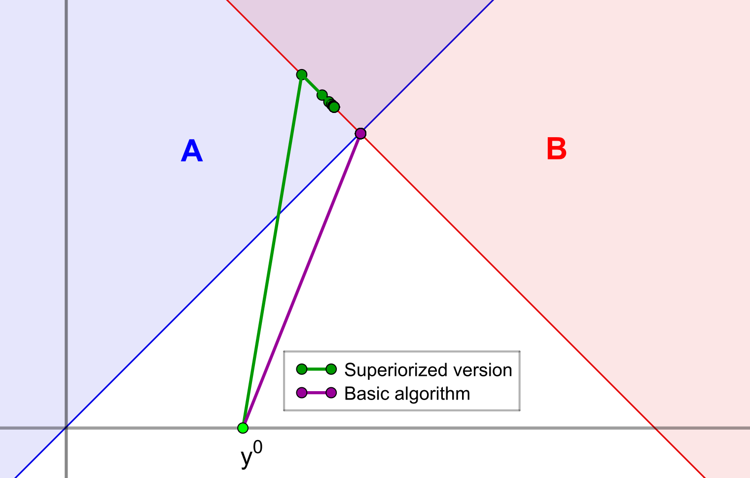
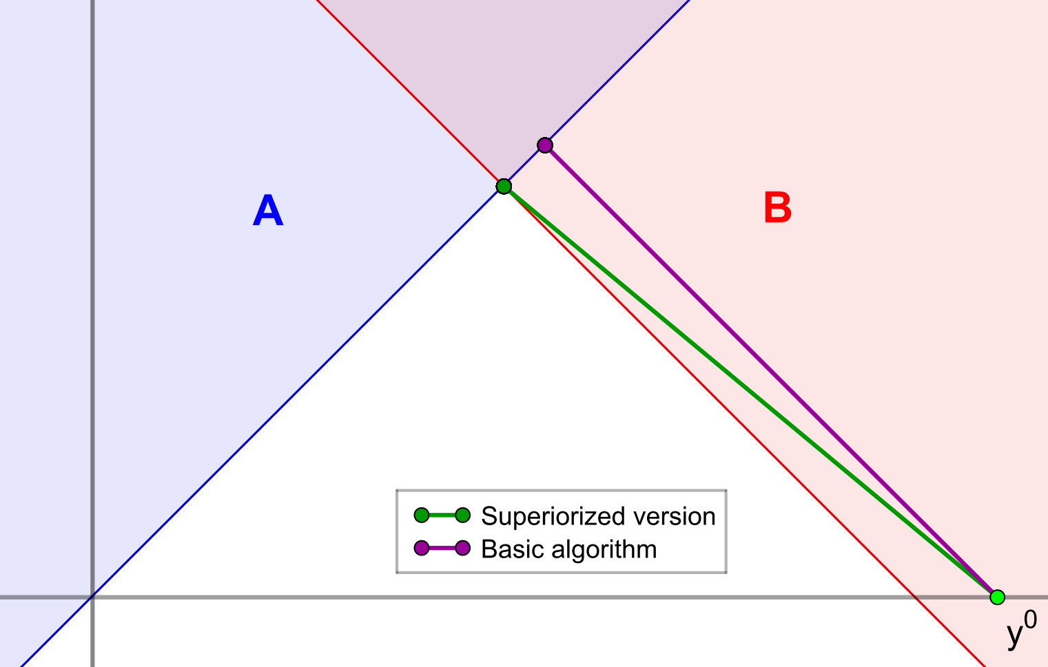
Figure 1: (Left) Taking $y^{0}=(3/10,0)^{T}$ as starting point, the alternating projection method converges in one iteration to the minimum norm point in the intersection of two half-spaces, while its superiorized version remains far from the solution after 50 iterations. (Right) If we take $y^{0}=(11/10,0)^{T},$ in one iteration, the superiorized version converges to the minimum norm point while the alternating projection method converges to a feasible point which is not the solution.

From this starting point the basic algorithm for feasibility-seeking alone without perturbations (i.e., the alternating projection method) converges in one iteration to the minimum norm point in the intersection of the two half-spaces, while its superiorized version remains far from the solution after 50 iterations. This happens because the first perturbation applied to this $y^{0}$ results in a point on the horizontal axis inside the set $A.$ If we were to choose another $y^{0}$ on the $x$-axis, but far enough to the right inside the set $B$, then after one perturbation the next point will be outside both sets $A$ and $B$ on the positive $x$-axis and this would lead, following a single iteration of feasibility-seeking, to the minimum norm point whereas the feasibility-seeking-only from that $y^{0}$ onward would lead to a less “superior” feasible point, as shown in Figure 1 (right).

Observe that we only computed 50 iterations because after them the norm of the perturbations is smaller than $2^{-50}\approx 8.9\cdot 10^{-16}$. Hence, the effect of the perturbations steering the basic algorithm to a superiorized solution vanishes, having no real effect on it after even less than 100 iterations. This phenomenon is inherent in the SM and the purpose of the restarts, proposed in the next section, is to improve this unwanted behavior.

In [32, Section 3] we gave a precise definition of the “guarantee problem” of the SM. We wrote there: “The SM interlaces into a feasibility-seeking basic algorithm target function reduction steps. These steps cause the target function to reach lower values locally, prior to performing the next feasibility-seeking iterations. A mathematical guarantee has not been found to date that the overall process of the superiorized version of the basic algorithm will not only retain its feasibility-seeking nature but also accumulate and preserve globally the target function reductions. We call this fundamental question of the SM “the guarantee problem of the SM” which is: under which conditions one can guarantee that a superiorized version of a bounded perturbation resilient feasibility-seeking algorithm converges to a feasible point that has target function value smaller or equal to that of a point to which this algorithm would have converged if no perturbations were applied – everything else being equal.”

Numerous works that are cited in [2] show that this global function reduction of the SM occurs in practice in many real-world applications. In addition to a partial answer in [32] with the aid of the “concentration of measure” principle there is also the partial result of [33, Theorem 4.1] about strict Fejér monotonicity of sequences generated by an SM algorithm.

3 First development: The superiorization method with perturbations restarts

We offer here a modification of the SM, applied to the superiorized version of the basic algorithm in Algorithm 2, by setting the perturbations step-sizes in a manner that allows restarts. Commonly, the summable sequence $\{\eta_{\ell}\}_{\ell=0}^{\infty}$ employed in Algorithm 2 is being generated by taking a real number $\alpha\in{]0,1[}$, referred to as kernel, and setting $\eta_{\ell}:=\alpha^{\ell}$, for $\ell\geq 0$. This strategy works well in practice, as witnessed by many works cited in [2], but it has though the inconvenience that, as the iterations progress, the step-sizes in (8) decrease toward zero quite fast, yielding insignificant perturbations.

In some applications, various methods have been studied for controlling the step-sizes, see, e.g., [10, 35, 36], see also the software package SNARK14 [37] which is an updated version of [38]. We propose here a new strategy which allows restarting the sequence of step-sizes to a previous value while maintaining the summability of the series of step-sizes. The restarting of step-sizes is a useful approach that allows to improve an algorithm’s performance, see, e.g. [39, 40], where this technique is applied to the stochastic gradient descent and FISTA, respectively.

Our proposed scheme for restarting the step-sizes is controlled by a sequence of positive integers $\{W_{r}\}_{r=0}^{\infty}$ and we call the indices $r=1,2,\ldots$ restart indices. Bearing some similarity to a backtracking scheme, the initial step-size at the beginning of a new loop of perturbations is reduced after each restart. Specifically, let $\alpha\in{]0,1[}$ be any fixed kernel, assume that $r$ restarts have been already performed and let $W_{r}$ denote the number of consecutive step-sizes which must be taken before allowing the next restart.

The algorithm begins with $r=0$ and takes $W_{0}$ decreasing step-sizes in the sequence $\{1,\alpha,\alpha^{2},\ldots\}$. After these $W_{0}$ step-sizes, the algorithm performs a restart in the step-sizes by setting $r=1$ and taking anew $W_{1}$ decreasing step-sizes in the sequence $\{\alpha,\alpha^{2},\alpha^{3},\ldots\}$. Then the algorithm performs another restart with $r=2$ and uses step-sizes in the sequence $\{\alpha^{2},\alpha^{3},\alpha^{4},\ldots\}$, and so on.

This is accurately described in the pseudo-code of the Superiorized Version of the Basic Algorithm with Restarts presented below. Observe that there are no restrictions on how the sequence $\{W_{r}\}_{r=0}^{\infty}$ is chosen. A simple possible choice is to take a positive constant value $W_{r}:=W$, for all $r\geq 0$.

Note that, since the kernel $\alpha$ needs to lie in the interval $]0,1[$, despite performing restarts, the perturbations may happen to yield an insignificant decrease in the objective value, specially if the norm of the nonascending vectors is close to zero. This can be controlled by considering a positive real number $c$ and performing the restarts to the sequence $\{c\,\alpha^{\ell}\}_{\ell=0}^{\infty}$ rather than to $\{\alpha^{\ell}\}_{\ell=0}^{\infty}$. This parameter is also included in the pseudo-code of Algorithm 3.

1 Initialization: Choose an arbitrary initialization point $y^{0}\in\mathbb{R}^{n}$, $\alpha\in{]0,1[}$, a positive number $c$, a positive integer $N$ and a sequence of positive integers $\{W_{r}\}_{r=0}^{\infty}$ ;

2 set $k=0$, $\ell=-1$, $w=0$ and $r=0$;

3 repeat

4     set $y^{k,0}=y^{k}$;

5      for $j=0$ to $N-1$ do

6           set $v^{k,j}$ to be a nonascending vector for $\phi$ at $y^{k,j}$;

7          set $\ell=\ell+1$;

8           while $\phi(y^{k,j}+c\,\alpha^{\ell}v^{k,j})>\phi(y^{k})$ do

9                set $\ell=\ell+1$;

10               

11                end while

12               set $y^{k,j+1}=y^{k,j}+c\,\alpha^{\ell}v^{k,j}$;

13               

14                end for

15               set $w=w+1$;

16                if $w=W_{r}$ then

17                     set $r=r+1$, $\ell=r$ and $w=0$;

18                    

19                     end if

20                    set $y^{k+1}=\mathbf{T}_{C}\left(y^{k,N}\right)$ and $k=k+1$;

21                    

22                    

23                    

Algorithm 3 The Superiorized Version of the Basic Algorithm with Restarts

Fact 6.

The strategy of restarts in Algorithm 3 preserves the summability of the overall series of step-sizes. This is so because even if during the iterative process, the largest step-sizes allowed in each of the sets $W_{r}$ were taken, then the infinite sequence of all step-sizes

$$\left(\left(\alpha^{r+\ell}\right)_{\ell=0}^{W_{r}-1}\right)_{r=0}^{\infty},$$ (13)

forms a bounded series. We have, since $\alpha\in{]0,1[}$,

$$\sum_{r=0}^{\infty}\sum_{\ell=0}^{W_{r}-1}\alpha^{r+\ell}\leq\sum_{r=0}^{\infty}\alpha^{r}\sum_{\ell=0}^{\infty}\alpha^{\ell}=\frac{1}{(1-\alpha)^{2}}.$$ (14)

Hence, since only step-sizes leading to expected superior values of the target function are allowed by (9) (line 8 of Algorithm 3), each of the step-sizes taken will be smaller than the corresponding one in the sequence (13), so its sum will always be smaller than $1/(1-\alpha)^{2}$ and will, thus, define bounded perturbations.

For some applications, the SM with restarts is very useful, notably outperforming the current SM without restarts (see Section 5.3).

4 Second development: A superiorized algorithm for subvectors in the split minimization problem

We develop here a superiorized algorithm for tackling the data of the SMP in Problem 1 when $C:=\bigcap_{s=1}^{p}C_{s}$ and $Q:=\bigcap_{t=1}^{q}Q_{t},$ where $p$ and $q$ are two integers and $\{C_{s}\}_{s=1}^{p}$ and $\{Q_{t}\}_{t=1}^{q}$ are two families of closed and convex sets with nonempty intersections in $\mathbb{R}^{n}$ and $\mathbb{R}^{m}$, respectively. To ease the discussion we will refer here to $\mathbb{R}^{n}$ and $\mathbb{R}^{m},$ as the “$x$-space” and the “$y$-space”, respectively.

4.1 The SMP with subvectors

In some situations of practical interest, the minimization problem in (2) should be independently applied to subvectors of the $y$-space. We discuss an instance in the field of radiation therapy treatment planning where this is significant in Section 5 below.

For simplicity and without loss of generality, we assume that the subvectors are in consecutive order. The $m\times n$ real matrix $A$ is divided into $B$ blocks and is represented by

$$A:=\left(\begin{array}[]{c}A_{1}\\ A_{2}\\ \vdots\\ A_{B}\end{array}\right)$$ (15)

where, for each $b\in B,$ $A_{b}\in\mathbb{R}^{m_{b}\times n}$ are blocks of rows of the matrix $A$, with $\sum_{b=1}^{B}m_{b}=m$. Thus, any vector $y:=Ax$ is of the form

$$y=\left(\begin{array}[]{c}y^{1}\\ y^{2}\\ \vdots\\ y^{B}\end{array}\right)=\left(\begin{array}[]{c}A_{1}\\ A_{2}\\ \vdots\\ A_{B}\end{array}\right)x$$ (16)

where $y^{b}\in\mathbb{R}^{m_{b}}$ are subvectors of $y\in\mathbb{R}^{m}.$

Problem 7.

The SMP with subvectors. Given two families of closed and convex sets $\{C_{s}\}_{s=1}^{p}\subseteq\mathbb{R}^{n}$ and $\{Q_{t}\}_{t=1}^{q}\subseteq\mathbb{R}^{m}$ such that $C:=\bigcap_{s=1}^{p}C_{s}\neq\emptyset$ and $Q:=\bigcap_{t=1}^{q}Q_{t}\neq\emptyset$, an $m\times n$ real matrix $A$ in the form (15) for a given integer $B$, a convex function $f:\mathbb{R}^{n}\to\mathbb{R}$ and convex functions and $\phi_{b}:\mathbb{R}^{m_{b}}\to\mathbb{R}$, for $b=1,2,\ldots,B$, find

$$x\in C\;\text{such that }x^{*}\in\operatorname*{argmin}\{f(x)\mid x\in C\},\;\text{ and such that}$$ (17)

$$y^{*}:=Ax^{*}\in Q\;\text{and}\;y^{b*}\in\operatorname*{argmin}\{\phi_{b}(y^{b})\mid y\in Q\}\;\text{ for all }\;b\in{\{1,2,\ldots,B\}}.$$ (18)

Our algorithm, presented below, can also handle subvectors in the $x$-space, but for simplicity we restrict ourselves here to subvectors in the $y$-space.

4.2 Reformulation in the product space

To work out a superiorization method for the data of the SMP with subvectors in Problem 7 we look at a multiple sets split feasibility problem (MSSFP), see, e.g., [41], as follows.

Problem 8.

The multiple sets split feasibility problem (MSSFP). Given $C:=\bigcap_{s=1}^{p}C_{s}$and $Q:=\bigcap_{t=1}^{q}Q_{t},$ where $p$ and $q$ are two integers, and $\{C_{s}\}_{s=1}^{p}$ and $\{Q_{t}\}_{t=1}^{q}$ are two families of closed and convex sets with nonempty intersections each in $\mathbb{R}^{n}$ and $\mathbb{R}^{m}$, respectively, and an $m\times n$ real matrix $A$, find

$$x^{*}\in C=\bigcap_{s=1}^{p}C_{s}\;\text{such that\;}y^{*}:=Ax^{*}\in Q=\bigcap_{t=1}^{q}Q_{t}.$$ (19)

This is a generalization of the split feasibility problem (SFP) that occurs when $p=q=1$ in the MSSFP. The SFP, which plays an important role in signal processing, in medical image reconstruction and in many other applications, was introduced by Censor and Elfving [42] in order to model certain inverse problems. Since then, many iterative algorithms for solving the SFP have been proposed and analyzed. See, for instance, the references given in [43] or consult the section “A brief review of ’split problems’ formulations and solution methods” in [44].

Our proposed algorithm deals with an equivalent reformulation of Problem 8 in the product space $\mathbb{R}^{n}$$\times$$\mathbb{R}^{m}$. Adopting the notation that quantities in the product space are denoted by boldface symbols, we define the sets

$$\mathbf{C}:=\left(\bigcap_{s=1}^{p}C_{s}\right)\times\left(\bigcap_{t=1}^{q}Q_{t}\right)\quad\text{and}\quad\mathbf{V}:=\{\mathbf{z}=(x,y)\in\mathbb{R}^{n}\times\mathbb{R}^{m}\mid Ax=y\}.$$ (20)

Note that the projection onto $\mathbf{V}$ is given by $P_{\mathbf{{V}}}=Z^{T}(ZZ^{T})^{-1}Z$, with $Z:=[A,-I]$, where $I$ denotes the $m\times m$ identity matrix. Then, Problem 8 is equivalent to the problem:

$$\text{find a point}\;\mathbf{z}^{*}\in\mathbf{C}\cap\mathbf{V}.$$ (21)

Without loss of generality, we assume that $p=q,$ since otherwise the whole space (or one particular set) could be added repeatedly as a constraint until both indices are equal. Since the projection of a Cartesian product is the Cartesian product of the projections [45, Lemma 1.1], the following implementation of the method of alternating projections can be employed to solve (21). We consider this as our basic algorithm for the superiorization method for subvectors.

1Initialization: Choose an arbitrary initialization point $x^{0}\in\mathbb{R}^{n}$. Set $y^{0}=Ax^{0}$;

Iterative Step: Given the current iterate $\mathbf{z}^{k}=(x^{k},y^{k})$, calculate the next iterate $\mathbf{z}^{k+1}$ by

$$\mathbf{z}^{k+1}=P_{\mathbf{V}}\left(\left(P_{C_{p}}\times P_{Q_{p}}\right)\cdots\left(P_{C_{1}}\times P_{Q_{1}}\right)(\mathbf{z}^{k})\right).$$ (22)

Algorithm 4 Basic Algorithm for the MSSFP.

In order to construct a superiorized version of Algorithm 4 that can cope with the data of the SMP with subvectors in Problem 7, we need to establish at each iteration some appropriate perturbations that will steer the algorithm to a superiorized solution. For this, we note that the vector $y^{k}$ inside $\mathbf{z}^{k}$ in (22) is expressed as

$$y^{k}=\left(\begin{array}[]{c}y^{1,k}\\ y^{2,k}\\ \vdots\\ y^{B,k}\end{array}\right)=\left(\begin{array}[]{c}A_{1}x^{k}\\ A_{2}x^{k}\\ \vdots\\ A_{B}x^{k}\end{array}\right).$$ (23)

Thus, we declare our perturbation vector to be

$$\left(\begin{array}[]{c}x^{k}\\ y^{k}\end{array}\right)+\eta_{k}\left(\begin{array}[]{c}u^{k}\\ v^{k}\end{array}\right),\quad\text{for all}\;k=0,1,2,\ldots,$$ (24)

where $\{\eta_{k}\}_{k=0}^{\infty}$ is a nonnegative summable sequence, $u^{k}$ is a nonascending vector for $f$ at $x^{k}$ and

$$v^{k}=\left(\begin{array}[]{c}v^{1,k}\\ v^{2,k}\\ \vdots\\ v^{B,k}\end{array}\right),$$ (25)

with each $v^{b,k}$ being a nonascending vector for $\phi_{b}$ at the point $A_{b}x^{k}$, for all $b\in{\{1,2,\ldots,B\}}$. The complete pseudo-code of the superiorized version of the basic Algorithm 4 with perturbations of the form given by (24) is shown in Algorithm 5.

1Initialization: Choose $x^{0}\in\mathbb{R}^{n}$, a summable nonnegative sequence $\{\eta_{\ell}\}_{\ell=0}^{\infty}$ and a positive integer $N$;

2 set $y^{b,0}=A_{b}x^{0}$ for $b\in{\{1,2\text{,}\ldots,B\}}$; set $k=0$ and $\ell=-1$;

3 repeat

4      set $x^{k,0}=x^{k}$;

5      set $y^{b,k,0}=y^{b,k}$ for $b\in{\{1,2\text{,}\ldots,B\}}$;

6      for $j=0$ to $N-1$ do

7           set $v_{x}^{k,j}$ to be a nonascending vector for $f$ at $x^{k,j}$;

8           set $v_{y}^{b,k,j}$ to be a nonascending vector for $\phi_{b}$ at the point $y^{b,k,j}$ for all $b$ ;

9           set $\ell=\ell+1$;

10           while $f(x^{k,j}+\eta_{\ell}v_{x}^{k,j})>f(x^{k})$ or there exists $b$ with $\phi_{b}(y^{b,k,j}+\eta_{\ell}v_{y}^{b,k,j})>\phi_{b}(y^{b,k})$ do

11                set $\ell=\ell+1$;

12               

13                end while

14               set $x^{k,j+1}=x^{k,j}+\eta_{\ell}v_{x}^{k,j}$;

15                set $y^{b,k,j+1}=y^{b,k,j}+\eta_{\ell}v_{y}^{b,k,j}$;

16               

17                end for

18               set $(x^{k+1},y^{1,k+1},\ldots,y^{B,k+1})=P_{\mathbf{V}}\left(\left(P_{C_{p}}\times P_{Q_{p}}\right)\cdots\left(P_{C_{1}}\times P_{Q_{1}}\right)\left(x^{k,N},y^{1,k,N},\ldots,y^{B,k,N}\right)\right)$ ;

19                set $k=k+1$;

20               

21               

22               

Algorithm 5 Superiorized Algorithm for the data of the SMP with subvectors

Since the method of alternating projections is bounded perturbation resilient [18], Algorithm 5 will converge to a solution of the feasibility problem (21). Moreover, by the nature of the SM, the algorithm is expected to converge to a point $\mathbf{z}^{*}=(x^{*},y^{*})$ which will be superior with respect to $f$ for the component $x$ in the $x$-space, and with respect to $\phi_{b}$ for the $b$-th subvector in the $y$-space, for $b=1,2,\ldots,B$.

5 Numerical experiments

Our aim in this paper is not to compare the superiorization method with constrained optimization methods, moreover, the SM is not a method intended to solve exact constrained optimization problems. Such comparisons were done elsewhere, see, e.g., [7] or [6]. Our goal is to show how the SM can be improved and this is achieved by comparing the SM with and without restarts and with and without perturbations. We present our results of numerical experiments performed on three different problems. The first two problems are simple illustrative examples. The computational performance of the SM with restart algorithms, proposed here, can be substantiated with exhaustive testing of the possible specific variants permitted by the general framework and their various user-chosen parameters. This should be done on larger problems, preferably within the context of a significant real-world application. Therefore, our third problem addresses an actual situation arising in the real-world application of intensity-modulated radiation therapy (IMRT) treatment planning.

The purpose of the first example is to illustrate the potential benefits of superiorization with restarts for finding a point with reduced norm in the intersection of two convex sets. We first consider the case of two balls and then explore the case of two half-spaces presented in Remark 2.1, in which superiorization did not achieve its purpose for a particular setting.

In the second example we illustrate the behavior of Algorithm 5 in a simple setting with $C,Q\subset\mathbb{R}^{2}$, where each of the sets is an intersections of three half-spaces.

Finally, the last experiment demonstrates the benefits of superiorization with restarts in a difficult realistic setting in IMRT, where a large-scale multiobjective optimization problem arises. All tests were run on a desktop of Intel Core i7-4770 CPU 3.40GHz with 32GB RAM, under Windows 10 (64-bit).

5.1 The benefits of superiorization with restarts

Consider the problem of finding the minimum norm point in the intersection of two balls $A$ and $B$ in the Euclidean 2-dimensional space, so $\phi:\mathbb{R}^{2}\to\mathbb{R}$ is given by $\phi(x):=\frac{1}{2}\|x\|^{2}$ for $x\in\mathbb{R}^{2}$. The underlying feasibility problem can be solved by the method of alternating projections, which we chose as the basic algorithm. Hence, the feasibility-seeking algorithmic operator used in our computations is

$$\mathbf{T}=P_{B}P_{A},$$ (26)

where $P_{A}$ and $P_{B}$ denote the projection operators onto the balls $A$ and $B,$ respectively. We tested the method of alternating projections, its superiorized version (with two different kernels $\alpha=0.6$ and $\alpha=0.999$) and its superiorized version with restarts (with $\alpha=0.6$ and $W_{r}=50$, for all $r\geq 0$). We set $N=1$ in all the superiorized algorithms. The nonascending directions were taken as $v^{k}:=-\frac{\nabla\phi(y^{k})}{\|\nabla\phi(y^{k})\|}=-\frac{y^{k}}{\|y^{k}\|}$.

The behavior of these algorithms is shown in Figure 2. On the left we represent 500 iterations generated by each algorithm. On the right, we plot the sequence of perturbations obtained before applying the algorithmic operator, that is, we draw the points $\left\{y^{k,N}\right\}_{k=0}^{500}$. This sequence coincides with the sequence of iterates $\left\{y^{k}\right\}_{k=0}^{500}$ in the case when no perturbations are performed at all and only the basic algorithm works, while it coincides with the sequence $\left\{y^{k}+\eta_{k}v^{k}\right\}_{k=0}^{500}$ for the superiorized algorithms.

As expected, the method of alternating projections converges to a point in the intersection which is not desirable according to the task of reducing the target function value (the squared norm). Superiorization with kernel $\alpha=0.6$ reaches a better point than the output of the basic algorithm, but is yet far from the solution to the problem. This might well be due to the step-sizes not being big enough for the perturbations to steer the algorithm to a proper function reduction.

Taking $\alpha=0.999$ in the standard superiorized version of the algorithm results in a very slow convergence of the algorithm, as can be observed on the right figure in Figure 2. These deficiencies are resolved by considering superiorization with restarts, which achieves fast convergence to a solution with reduced norm in the intersection.

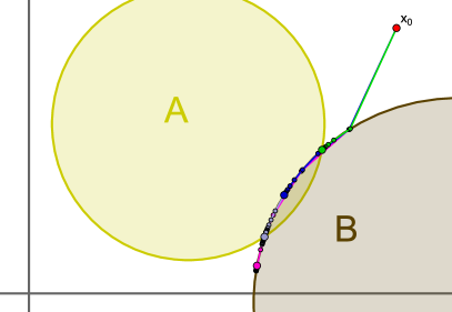
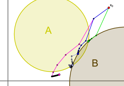
Figure 2: Behavior of the different algorithms considered applied to the data of the problem of finding the minimum norm point in the intersection of the balls $A$ and $B$. The figures show the first 500 points in the sequence of iterates $\{y^{k}\}_{k=0}^{500}$ (left) and the sequence of perturbed iterations before applying the algorithmic operator $\{y^{k,N}\}_{k=0}^{500}$ (right) of each algorithm.

The example presented in Section 2.1 is artificial in the sense that the vectors defining the half-spaces are orthogonal and the starting point was chosen in a particular region of the plane which was less favorable to the superiorized algorithm. Also, the value of the kernel was chosen to be small ($\alpha=0.5$), to aggravate the vanishing effect of the perturbations.

To investigate what happens with random data, we ran an experiment generating $1\,000\,000$ pairs of half-spaces of the form $A:=\left\{x\in\mathbb{R}^{2}\mid\left\langle c_{A},x\right\rangle\leq b_{A}\right\}$ and $B:=\left\{x\in\mathbb{R}^{2}\mid\left\langle c_{B},x\right\rangle\leq b_{B}\right\}$ where the vectors $c_{A},c_{B}\in\mathbb{R}^{2}$ were randomly chosen and then normalized, and $b_{A},b_{B}\in(-1,0)$ (to ensure that $(0,0)^{T}\not\in A\cap B$). For each pair of half-spaces, we generated a random starting point $y^{0}\in[-1,1]^{2}$ such that $y^{0}\not\in A\cap B$.

Then, we ran from $y^{0}$ the basic algorithm (feasibility-seeking alternating projections), its superiorized version with kernel $\alpha\in\left\{0.5,0.6,0.7,0.8,0.9\right\}$ and its superiorized version with restarts with $W_{r}=20$ and $N=1$. The results are summarized in Table 1. In this table AP stands for “alternating projections”, Sup stands for “the superiorized version”, and Sup. Res. stands for “the superiorized version with restarts”. We count that one method is better than the other when the norm of its solution is smaller than the norm of the second method’s output minus $10^{-3}$. With kernel $\alpha=0.5$, the superiorized algorithm failed to obtain a solution with lower norm than the basic algorithm in $12\,931$ of the $1\,000\,000$ instances; with kernel $\alpha=0.9$, this number was reduced to 122. The superiorized algorithm with restarts with kernel $\alpha=0.7$ only failed to get a better solution than the basic algorithm in 21 instances. Remarkably, when the kernels $\alpha\in\left\{0.8,0.9\right\}$ were used, superiorization with restarts always reached the same or a better solution than both the basic and the superiorized algorithms without restarts.

	AP vs Sup.		AP vs Sup. Res.			Sup. vs Sup. Res.
Kernel	AP	Sup.	AP	Sup.	Res.	Sup.	Sup.	Res.
$\alpha=0.5$	1.29%	56.17%	0.08%	57.	2%	0.01%	16.	9%
$\alpha=0.6$	0.73%	56.63%	0.02%	57.	26%	0.001%	10.	78%
$\alpha=0.7$	0.32%	56.96%	0.002%	57.	28%	0%	6.	1%
$\alpha=0.8$	0.10%	57.17%	0%	57.	29%	0%	2.	86%
$\alpha=0.9$	0.01%	57.27%	0%	57.	3%	0%	0.	68%

Table 1: For each pair-wise comparative of methods and kernel choice, the numbers inside the table are the percentage of the $1\,000\,000$ runs in which each method obtains a solution with lower norm than the other one with which it is compared.

5.2 Behavior of the superiorized algorithm for the data of the SMP

In this section we present another illustrative example of the performance of Algorithm 5. To be able to display the iterates, we let both the $x$-space and the $y$-space in Problem (17)-(18) be the Euclidean 2-dimensional spaces. We take $C$ as the intersection of the three half-spaces given by $C_{1}:=\left\{(x_{1},x_{2})\in\mathbb{R}^{2}\mid x_{1}+x_{2}\leq 10\right\}$, $C_{2}:=\left\{(x_{1},x_{2})\in\mathbb{R}^{2}\mid-13x_{1}+3x_{2}\leq-26\right\}$ and $C_{3}:=\left\{(x_{1},x_{2})\in\mathbb{R}^{2}\mid x_{2}\geq 1\right\}$.

We let $A$ be the rotation matrix by an angle of $\pi/2$ and $Q$ be the image of $C$ under $A$ (i.e., the intersection of the half-spaces $Q_{1}:=\left\{(y_{1},y_{2})\in\mathbb{R}^{2}\mid y_{1}-y_{2}\leq-10\right\}$, $Q_{2}:=\left\{(y_{1},y_{2})\in\mathbb{R}^{2}\mid-3y_{1}-13y_{2}\leq-26\right\}$ and $Q_{3}:=\left\{(y_{1},y_{2})\in\mathbb{R}^{2}\mid y_{1}\leq-1\right\}$). The function to be reduced in the $x$-space is the value of the second component $f(x_{1},x_{2}):=x_{2}$, whereas in the $y$-space, we aim to find a point with increased first and second components (that is, $B:=2$, $\phi_{1}(y_{1}):=-y_{1}$ and $\phi_{2}(y_{2}):=-y_{2}$).

In other words, we want to tackle with the SM the data of the split minimization problem given by

$$\text{find }x^{*}=\left(\begin{array}[]{c}x_{1}^{*}\\ x_{2}^{*}\end{array}\right)\in C\text{ such that }x^{*}\in\operatorname*{argmin}{\left\{x_{2}\;\Bigl{|}\;\left(\begin{array}[]{c}x_{1}\\ x_{2}\end{array}\right)\in C\right\}}$$ (27)

$$\textup{and such that }\left(\begin{array}[]{c}-x_{2}^{*}\\ x_{1}^{*}\end{array}\right)\in Q,\quad-x_{2}^{*}\geq y_{1}\text{ and }x_{1}^{*}\geq y_{2}\text{ for all }\left(\begin{array}[]{c}y_{1}\\ y_{2}\end{array}\right)\in Q,$$ (28)

with $C:=\bigcap_{i=1}^{3}C_{i}$ and $Q:=\bigcap_{j=1}^{3}Q_{j.}$

By looking at Figure 3, one easily identifies that the point $(9,1)^{T}$, obtained as the intersection of the lines $x_{1}+x_{2}=10$ and $x_{2}=1$, is the unique solution to the SMP with the above described data.

Again, for the SM we choose the method of alternating projections as the basic algorithm. Consequently, the algorithmic operator that we use is

$$\mathbf{T}:=P_{\textbf{V}}\circ\left(P_{C_{3}}\times P_{Q_{3}}\right)\circ\left(P_{C_{2}}\times P_{Q_{2}}\right)\circ\left(P_{C_{1}}\times P_{Q_{1}}\right),$$ (29)

where we recall that $\mathbf{V}:=\left\{(x,y)\in\mathbb{R}^{2}\times\mathbb{R}^{2}\mid Ax=y\right\}$. In our experiment, we performed 50 iterations of both the basic algorithm and its superiorized version, taking $\alpha=0.9$ as the kernel for generating the step-sizes of the perturbations and $N=1$. The nonascending vectors were taken as $v_{x}^{k}:=(0,1)^{T}$ for the perturbations in the $x$-space, and $v_{y}^{1,k}:=1$ and $v_{y}^{2,k}:=1$ in the $y$-space.

Figure 3 shows that, while the method of alternating projection converges to the closest point to the starting point in the intersection in each of the spaces, the superiorized algorithm converges to the solution of the SMP.

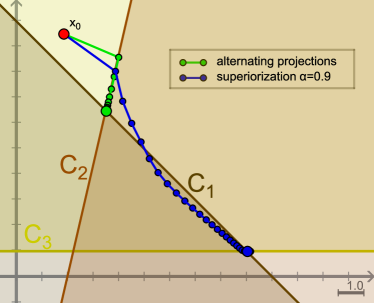
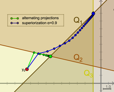
Figure 3: Performance of the method of alternating projections and its superiorized version applied in the setting of problem (27)-(28). The left image displays the iterates in the $x$-space, while the right one shows the iterates in the $y$-space.

5.3 A demonstrative example in IMRT

In this section, we test our SM with restarts algorithm in a sophisticated multiobjective setting motivated from a split minimization problem in the field of intensity-modulated radiation therapy (IMRT) treatment planning. IMRT is a radiation therapy that manipulates particle beams (protons or photons or others) of varying directions and intensities that are directed toward a human patient to achieve a goal of eradicating tumorous tissues, henceforth called “tumor structures”, while keeping healthy tissues, called “organs-at-risk” below certain thresholds of absorbed dose of radiation. The beams are projected onto the region of interest from different angles.

Many review papers in this field are available, see, e.g., [46, 47, 48, 49, 50] and references therein.

5.3.1 The fully-discretized model of the inverse problem of IMRT

In the fully-discretized model of the inverse problem of IMRT each external radiation beam is discretized into a finite number of “beamlets” (also called “pencil-beams” or “rays”) along which the particles (i.e., their energies) are transmitted. Let all beamlets from all directions be indexed by $i=1,2,\ldots,n,$ and denote the “intensity” irradiated along the $i$-th beamlet by $x_{i}$. The vector $x=(x_{i})_{i=1}^{n}\in\mathbb{R}^{n}$ is called the “intensities vector”.

The 2-dimensional (2D) cross-section of the irradiated body is discretized. Assume that the cross-section is covered by a square that is discretized into a finite number of square pixels. This creates an $M\times M$ array of pixels. Let all pixels be indexed by $j=1,2,\ldots,m,$ with $m=M^{2}$ and let $y_{j}$ denote the “dose” of radiation absorbed in the $j$-th pixel. The vector $y=(y_{j})_{j=1}^{m}\in\mathbb{R}^{m}$ is called the “dose vector”.

The “intensities space” $\mathbb{R}^{n}$ and the “dose space” $\mathbb{R}^{m},$ defined above are the “$x$-space” and the “$y$-space”, respectively, mentioned at the beginning of Section 4. The physics of the model assumes that there exists an $m\times n$ real matrix $A=(a_{ij})_{i=1,j=1}^{n,m}$(sometimes called “the dose matrix”) through which the intensities of the beamlets and the absorbed doses in pixels are related via the equation

$$Ax=y.$$ (30)

Each element $a_{ij}$ in $A$ is the dose absorbed in pixel $j$ due to a unit of intensity along the $i$-th beamlet. This means that

$$\sum_{i=1}^{n}a_{ij}x_{i}$$ (31)

is the total dose absorbed in pixel $j$ due to an intensity vector $x$. With these notions in mind we consider the following feasibility-seeking problem of the fully-discretized inverse problem of IMRT.

Problem 9.

The feasibility-seeking problem of the fully-discretized inverse problem of IMRT. Let $\mathbb{R}^{n}$ and $\mathbb{R}^{m}$ be the “intensities space” and the “dose space” (henceforth called the “$x$-space” and the “$y$-space”) respectively. Let $A=(a_{ij})_{i=1,j=1}^{n,m}$ be the dose matrix mapping the $x$-space onto the $y$-space. For $\ell=1,2,\ldots,L$, denote by $T_{\ell}\subseteq\{1,2,\ldots,m\}$ the set of pixels corresponding to the $\ell$-th tumor structure in the region of interest. For $r=1,2,\ldots,R$, denote by $S_{r}\subseteq\{1,2,\ldots,m\}$ the set of pixels corresponding to the $r$-th organ-at-risk. Set $\underline{e}$ and $\overline{e}$ the lower and upper bounds for the available beamlets intensities. Let $\underline{d}_{r}$ and $\overline{d}_{r}$, and $\underline{c}_{\ell}$ and $\overline{c}_{\ell}$ be the lower and upper bounds for the dose deposited in each pixel of the $r$-th organ at risk and of the $\ell$-th tumor, respectively.

The task is to find an intensities vector $x$ such that

$$\underline{c}_{\ell}\leq\sum_{i=1}^{n}a_{ij}x_{i}\leq\overline{c}_{\ell}, \quad\text{ for all }j\in T_{\ell},\quad\ell\in{\{1,2,\ldots,L\}},$$ (32)

$$\underline{d}_{r}\leq\sum_{i=1}^{n}a_{ij}x_{i}\leq\overline{d}_{r}, \quad\text{ for all }j\in S_{r},\quad r\in{\{1,2,\ldots,R\}},$$

$$\underline{e}\leq x_{i}\leq\overline{e}, \quad\text{ for all }i\in{\{1,2,\ldots,n\}}.$$

Problem 9 is a linear feasibility problem. Usually, $\underline{e}=\underline{d}_{r}=0$ and the significant bounds are $\underline{c}_{\ell}$ for tumor structures and $\overline{d}_{r}$ for organs-at-risk. A pair $(x^{*},y^{*})$ such that $x^{*}$ is a solution of Problem 9 and $y^{*}=Ax^{*}$ will be henceforth called “a treatment plan” for the IMRT inverse planning problem.

5.3.2 The quest for smoothness and uniformness

In the IMRT inverse planning problem there is an advantage to generating treatment plans with intensity vectors $x^{*}$ whose subvectors, related to parallel beamlets from the same beam, will be as “smooth” as possible and with dose vectors $y^{*}$ whose subvectors, related to specific organs (a.k.a. “structures”), that will be as “uniform” as possible.

For the intensity vectors $x^{*},$ “smoothness” of subvectors, related to parallel beamlets from the same beam, means that the real numbers that are the individual intensities $x_{i}^{*}$, in each subvector separately, would be as close to each other as possible, subject to the constraints of Problem 9. Such smoothness will allow for less extreme movements of the “multileaf collimator” (MLC) that modulates the parallel beamlets from the same beam.

For the dose vectors $y^{*},$ “uniformness” of subvectors, related to specific organs means that the real numbers that are the individual doses $y_{j}^{*}$, in each pixel of the subvector would be as close to each other as possible, subject to the constraints of Problem 9. Such uniformness will guarantee uniformness of the dose deposited within each organ separately and help to avoid the presence of hot- and cold-spots in the dose distribution in each organ. See, e.g., [52].

Each of these aims can be achieved by attempting to minimize or just reduce the total variation (TV)-norm of the associated subvectors, see, e.g., [53] for a general work on the $TV$-norm. For an $M\times M$ array $z=(z_{s,t})_{s=1,t=1}^{M,M}$ the $TV$-norm is defined as the convex function $TV:\mathbb{R}^{M\times M}\to\mathbb{R}$ given by

$$TV(z):=\sum_{s=1}^{M-1}\sum_{t=1}^{M-1} \sqrt{(z_{s,t}-z_{s+1,t})^{2}+(z_{s,t}-z_{s,t+1})^{2}}$$ (33)

$$\quad+\sum_{s=1}^{M-1}|z_{s,M}-z_{s+1,M}|+\sum_{t=1}^{M-1}|z_{M,t}-z_{M,t+1}|.$$

Choosing the $TV$-norm as the objective function in the “$x$-space” or the “$y$-space”, or both, and associating it with the feasibility-seeking problem of the fully-discretized inverse problem of IMRT (Problem 9) leads naturally to formulations of the SMP in Problem 1.

5.3.3 The experimental setup

For the purpose of our numerical experiment we confine ourselves specifically to a case of the feasibility-seeking problem of the fully-discretized inverse problem of IMRT (Problem 9) where there are $L$ tumor structures and the whole rest of the cross-section is considered as one single organ-at-risk, i.e., we let $S_{r}=S\subseteq\{1,2,\ldots,m\}$ for all $r=1,2,\ldots,R.$ This leads to the next split problem of minimizing the $TV$-norm of the dose subvectors so that uniformity of dose distribution will be achieved for each tumor structure separately.

Problem 10.

Let $\mathbb{R}^{n}$ be the $x$-space of intensity vectors, let $\mathbb{R}^{m}$ be the $y$-space of dose vectors, and $A$ be the dose matrix relating them to each other. For $\ell=1,2,\ldots,L$ denote by $T_{\ell}\subseteq\{1,2,\ldots,m\}$ the sets of pixels corresponding to the $\ell$-th tumor structure and let $S\subseteq\{1,2,\ldots,m\}$ be the complementary set of pixels that do not belong to any of the target structures and represent all organs at risk. Set $0$ and $\overline{e}$ the lower and upper bounds for the beamlets intensities. Let $\underline{d}$ and $\overline{d}$, and $\underline{c}_{\ell}$ and $\overline{c}_{\ell}$ be the dose bounds for pixels in an organ-at-risk and at the tumor structures, respectively. We further assume that the dose vector $y=Ax$ consists of $L+1$ subvectors $y=(y^{\ell})_{\ell=1}^{L+1}$such that the first $L$ subvectors consists of the doses absorbed in pixels of the $L$ tumor structures and $y^{L+1}$ is the dose absorbed in the complementary tissue $S.$

The task is to find an intensities vector $x$ such that

$$\underline{c}_{\ell}\leq y_{j}^{\ell}=\sum_{i=1}^{n}a_{ij}x_{i}\leq\overline{c}_{\ell}, \quad\text{ for all }j\in T_{\ell},\quad\ell\in{\{1,2,\ldots,L\}},$$ (34)

$$\underline{d}\leq y_{j}^{L+1}=\sum_{i=1}^{n}a_{ij}x_{i}\leq\overline{d}, \quad\text{ for all }j\in S,$$

$$\underline{e}\leq x_{i}\leq\overline{e}, \quad\text{ for all }i\in{\{1,2,\ldots,n\}},$$

$$\text{ and }y^{\ell}\in\operatorname*{argmin}\{TV(u)\>|\>u\in[\underline{c}_{\ell},\overline{c}_{\ell}]^{|T_{\ell}|}\}\text{ for all }\ell\in{\{1,2,\ldots,L\}},$$ (35)

where, for every $\ell\in{\{1,2,\ldots,L\}}$, $y^{\ell}$ denotes the subvector of the vector $y$ associated with the $\ell$-th tumor, and $|T_{\ell}|$ is the cardinality of the set $T_{\ell}$.

This is the problem we worked on in our experiment. We do not use real data but replicate a realistic situation. In particular, we consider a cross-section of $50\times 50$ square pixels, which translates into the dose vector in the $y$-space $\mathbb{R}^{2500}$. The number of external radiation beamlets is $n=2840$, meaning that the $x$-space is $\mathbb{R}^{2840}$. In the cross-section we have two tumor structures of irregular shapes, whose location appears in Figure 4. In order to guarantee the existence of a feasible solution for Problem 10, we generated the data as follows.

• We generate a vector $\overline{y}\in\mathbb{R}^{2500}$ with components randomly distributed in the interval $[0,15]$ for the pixels corresponding to organs-at-risk, and in the interval $[10,40]$ for pixels of tumor structures.

• We randomly generated a matrix $V\in\mathbb{R}^{2840\times 2500}$ with entries in the interval $[0,1]$ and defined the dose matrix $A\in\mathbb{R}^{2500\times 2840}$, mapping the $x$-space onto the $y$-space, as the generalized left inverse of $V$, i.e., we took $A:=(V^{T}V)^{-1}V^{T}$.

• We defined $\overline{x}:=V\overline{y}$, which implies that $\overline{y}=A\overline{x}$.

• We set the bounds for the constraints of Problem 10 as

  $$\left\{\begin{array}[]{l}\underline{d}=0,\,\overline{d}=\max\{\overline{y}_{j}\mid j\in S\}+5\varepsilon_{1},\\ \underline{c}_{1}=\min\{\overline{y}_{j}\mid j\in T_{1}\}-5\varepsilon_{2},\,\overline{c}_{1}=\max\{\overline{y}_{j}\mid j\in T_{1}\}+5\varepsilon_{3},\\ \underline{c}_{2}=\min\{\overline{y}_{j}\mid j\in T_{2}\}-5\varepsilon_{4},\,\overline{c}_{2}=\max\{\overline{y}_{j}\mid j\in T_{2}\}+5\varepsilon_{5},\\ \underline{e}=(\varepsilon_{6}+1)/2\min\{\overline{x}_{i}\mid i\in{\{1,2,\ldots,n\}}\},\\ \overline{e}=(1+\varepsilon_{7}/2)\max\{\overline{x}_{i}\mid i\in{\{1,2,\ldots,n\}}\},\end{array}\right.$$ (36)

  where the sub-indices in $\overline{c}$ and $\underline{c}$ refer to the first and second tumor structures and, for $i\in{\{1,2,\ldots,7\}}$, $\varepsilon_{i}$ are randomly picked real numbers in the interval $(0,1]$.

These choices during the data generation guarantee that there exists a feasible solution for Problem 10 with these data, namely $\overline{x}$.

In our experimental work, we ran the basic algorithm (Algorithm 4) and the superiorized version of the basic algorithm (Algorithm 5) with and without restarts. For all of them we took the algorithmic operator as

$$\mathbf{T}:=P_{\textbf{V}}\circ\left(P_{[\underline{e},\overline{e}]}\times P_{Q}\right),$$ (37)

with $\mathbf{V}:=\left\{(x,y)\in\mathbb{R}^{n}\times\mathbb{R}^{m}\mid Ax=y\right\}$ and $P_{Q}:\mathbb{R}^{m}\rightarrow\mathbb{R}^{m}$ defined component-wise as

$$P_{Q}(y_{j}):=\left\{\begin{array}[]{l}P_{[\underline{d},\overline{d}]},\text{ if }j\in S,\\ P_{[\underline{c}_{1},\overline{c}_{1}]},\text{ if }j\in T_{1},\\ P_{[\underline{c}_{2},\overline{c}_{2}]},\text{ if }j\in T_{2}.\end{array}\right.$$ (38)

We tested the three algorithms with different choices of the parameters and present here the most advantageous for each one. Specifically, in Algorithm 5 with or without restart the step-sizes were taken in the sequence $\{c\,\alpha^{\ell}\}_{\ell=0}^{\infty}$ with a constant kernel $\alpha$ and a positive number $c$, and we took $N=5$. We performed some experiments in order to determine the best choice of $\alpha$ and $c$ for each method. The results are shown in Table 2. We chose $\alpha=0.999$ and $c=100\,000$ for the superiorized algorithm, since these parameters provide the best reduction in $TV$-norm values while performing the fastest. For the superiorization with restarts, all of the combinations of parameters, except of the first one, provide a great reduction in the $TV$-norm values with respect to superiorization with no restarts. Among these combinations, $\alpha=0.99$ and $c=100$ was the fastest, so we opted for it.

The target functions $\phi_{b}$ were always the appropriate $TV$-norms. Since no smoothing of the intensities vectors is included in the experiment, we took $v_{x}^{k,j}=0,$ for all $k$ and $j$. The final parameters of the two methods are the following:

• Superiorization: We took $\alpha=0.999$, $c=100\,000$ and $N=5$, and $v_{y}^{k,b,j}$ was defined as the nonascending direction given by Theorem 5.

• Superiorization with restarts: We took $\alpha=0.99$, $c=100$, $W_{r}=20$ for all $r$ and $N=5$, and $v_{y}^{k,b,j}$ was defined as the nonascending direction given by Theorem 5.

		$\alpha=0.99$					$\alpha=0.999$
		$c=10$	$c=100$	$c=1000$	$c=10\,000$	$c=100\,000$	$c=10$	$c=100$	$c=1000$	$c=10\,000$	$c=100\,000$
Sup.	$TV1$	2433.38	2433.36	2432.93	2430.40	2430.40	2432.26	2423.20	2300.88	2167.01	2166.97
	$TV2$	3056.41	3056.34	3055.51	3052.28	3052.28	3054.67	3039.15	2899.47	2714.62	2714.58
	Time	204.34	202.87	203.46	201.12	208.12	202.69	201.84	199.67	199.33	196.57
Sup. Restarts	$TV1$	2078.81	368.81	397.35	381.65	371.03	249.96	361.70	386.13	381.51	382.51
	$TV2$	2689.98	707.2	598.24	579.47	568.02	585.33	583.39	534.21	528.54	528.56
	Time	367.65	453.47	598.55	779.16	950.63	2362.15	3560.19	4426.75	6181.23	7174.09

Table 2: Average $TV$-norm values for the first and second subvectors and average time (in seconds) obtained by running the Superiorized and Superiorized with restarts algorithm with different choices of parameters for 10 random initial points. The algorithms were stopped when a proximity of 0.01 was reached.

We performed multiple runs of the three algorithms. At each run, each of the algorithms was initialized at the same starting point which was randomly generated in the interval $[\underline{e},\overline{e}]$. We define the proximity of an iterate as the distance to the feasible region, i.e., for an iterate pair $(x^{k},y^{k})$, we define its proximity as

$${\rm prox}(x^{k},y^{k}):=\|x^{k}-P_{[\underline{e},\bar{e}]}(x^{k})\|+\|y^{k}-P_{Q}(y^{k})\|.$$ (39)

Note that, due to the definition of the algorithmic operator $\mathbf{T}$, the distance of $(x^{k},y^{k})$ to $\mathbf{V}$ is $0$. All three algorithms were terminated once the proximity became less than $0.01$. The obtained results for all different runs are summarized in Table 3. Our numerical experiments showed that superiorization with restarts was considerably the best performing algorithm regarding the target function reduction, while superiorization alone, without restarts, did not achieve a significant reduction with respect to the basic algorithm.

This fact can be graphically observed in the heat maps of Figure 4, where we represent the dose in the pixels of the cross-section at the last iteration of each algorithm. The uniformity of the heat distribution in a tumor structure represents the dose distribution in that structure. Clearly, superiorization with restarts provided a more homogeneous dose distribution in the tumorous pixels. We observed the increased uniformity of dose distributions in the tumors in all our algorithmic runs of the superiorization with restarts method. However, depending on the datasets and the allowable parameters the level of the uniformity may vary.

The evolution along the iterations of the proximity and the total variation of the algorithms is shown in Figure 5 with “proximity-target function curves” (which were introduced in [54]), where the iteration indices $k$ increase from right to left in each of the plots. Finally, we note that superiorization with restarts needed more time and a larger number of iterations to reach the desired proximity.

In our experiments we have observed that other choices of parameters for the superiorization with restarts runs can be employed to reduce its running times and make them comparable to those of the superiorized algorithm without restarts and, at the same time, still achieve a significant reduction of the target function when compared to the other algorithms.

Run		1		2		3		4		5
$TV$ for subvector 1	Basic	2405.	3	2498.	4	2289.	3	2624.	74	2474.	9
	Superiorized	2072.	8	2230.	1	2089.	6	2362.	7	227.	2
	Sup. Restarts	421.	9	315.	6	404.	3	349.	3	301.	1
$TV$ for subvector 2	Basic	3019.	1	3252.	8	3002.	5	3076.	6	3096.	3
	Superiorized	2703.	3	2837.	4	2558.	9	2744.	3	2848.	2
	Sup. Restarts	817.	7	759.	7	688.	1	709.	2	531.	2
Run time (sec.)	Basic	96.	1	94.	6	91.	6	93.	6	95.	4
	Superiorized	261.	6	263.	3	253.	8	269.	4	267.	3
	Sup. Restarts	577.	5	588.	0	630.	9	580.	3	582.	7
No. of iterations	Basic	7352		7265		7117		7400		7505
	Superiorized	7327		7195		7095		7382		7478
	Sup. Restarts	14880		14819		17140		15275		14778

Table 3: $TV$-norm values for the first and second subvector, run times and number of iterations resulting from running the Basic, Superiorized and Superiorized with restarts algorithms (for runs with 5 different random initial points) until a proximity of $0.01$ was reached.

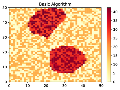
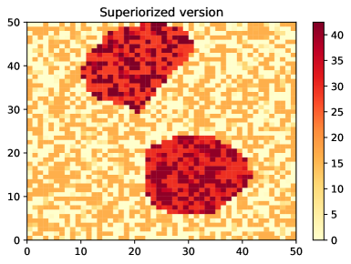
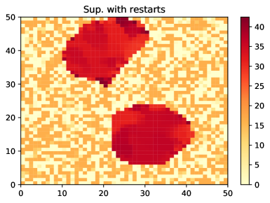
Figure 4: Heat maps of the solutions in the $y$-space of pixel doses for the first run of each one of the studied algorithms. Represented is a $50\times 50$ square grid of pixels, where the color indicates the dose absorbed in each pixel.

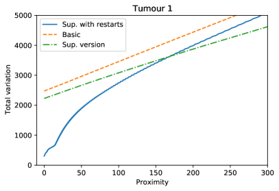
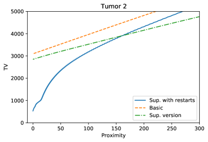
Figure 5: The evolution of the total variation and the proximity of the iterations of the first run of each of the algorithms for the subvector associated to the first tumor (left) and the second tumor (right). In these “proximity-target function curves” the iteration indices $k$ increase from right to left in each of the plots.

References

- [1] A. Beck, M. Teboulle, A fast iterative shrinkage-tresholding algorithm for linear inverse problems, SIAM J. Imaging Sci. 2 (2009), 138–202.
-
[2]
Y. Censor,
Superiorization and
perturbation resilience of algorithms: A bibliography compiled and
continuously updated.
Online at:
http://math.haifa.ac.il/yair/bib-superiorization-censor.html (last updated: July 28, 2022.) - [3] Y. Censor, Weak and strong superiorization: Between feasibility-seeking and minimization, Analele Stiint. ale Univ. Ovidius Constanta Ser. Mat., 23 (2015), 41–54.
- [4] T. Humphries, J. Winn, A. Faridani, Superiorized algorithm for reconstruction of CT images from sparse-view and limited-angle polyenergetic data, Phys. Med. Biol. 62 (2017), 6762.
- [5] G.T. Herman, Problem structures in the theory and practice of superiorization, J. Appl. Num. Optim. 2 (2020), 71–76.
- [6] Y. Censor, R. Davidi, G.T. Herman, R.W. Schulte, L. Tetruashvili, Projected subgradient minimization versus superiorization, J. Optim. Theory Appl. 160 (2014), 730–747.
- [7] M. Guenter, S. Collins, A. Ogilvy, W. Hare, A. Jirasek, Superiorization versus regularization: A comparison of algorithms for solving image reconstruction problems with applications in computed tomography, Med. Phys. 49 (2022), 1065–1082.
- [8] R. Davidi, Y. Censor, R.W. Schulte, S. Geneser, L. Xing, Feasibility-seeking and superiorization algorithms applied to inverse treatment planning in radiation therapy, Contemp. Math. 636 (2015), 83–92.
- [9] W. Jin, Y. Censor, M. Jiang, A heuristic superiorization-like approach to bioluminescence, International Federation for Medical and Biological Engineering (IFMBE) Proceedings 39 (2013), 1026–1029.
- [10] Y. Censor, Can linear superiorization be useful for linear optimization problems?, Inverse Probl. 33 (2017), 044006.
- [11] Y. Censor, S. Petra and C. Schnörr, Superiorization vs. accelerated convex optimization: The superiorized/regularized least-squares case, J. Appl. Math. Optim. 2 (2020), 15–62.
- [12] Y. Censor, A. Gibali, S. Reich, Algorithms for the split variational inequality problem, Numer. Algorithms 59 (2012), 301–323.
- [13] J.P. Boyle, R.L. Dykstra, A method for finding projections onto the intersection of convex sets in Hilbert spaces, in: R. Dykstra, T. Robertson, F.T. Wright (Eds.), Advances in Order Restricted Statistical Inference, Lecture Notes in Statistics, vol. 37. Springer, New York, 1986, pp. 28–47.
- [14] H.H. Bauschke, P.L. Combettes, Convex Analysis and Monotone Operator Theory in Hilbert Spaces, second edition. Springer, Berlin, 2017.
- [15] H.H. Bauschke, The approximation of fixed points of compositions of nonexpansive mappings in Hilbert space, J. Math. Anal. Appl. 202 (1996), 150–159.
- [16] F.J. Aragón Artacho, R. Campoy, A new projection method for finding the closest point in the intersection of convex sets, Comput. Optim. Appl. 69 (2018), 99–132.
- [17] R. Davidi, G.T. Herman, Y. Censor, Perturbation-resilient block iterative projection methods with application to image reconstruction from projections, Int. Trans. Oper. Res. 16 (2009), 505–524.
- [18] D. Butnariu, R. Davidi, G.T Herman, I.G. Kazantsev, Stable convergence behavior under summable perturbations of a class of projection methods for convex feasibility and optimization problems, IEEE J. Sel. Topics Signal Process. 1 (2007), 540–547.
- [19] D. Butnariu, S. Reich, A.J. Zaslavski, Convergence to fixed points of inexact orbits of Bregman-monotone and of nonexpansive operators in Banach spaces, in: H.F. Nathansky, B.G. de Buen, K. Goebel, W.A. Kirk, B. Sims (Eds.), Fixed Point Theory and its Applications, (Conference Proceedings, Guanajuato, Mexico, 2005), Yokahama Publishers, Yokahama, Japan, 2096, pp. 11–32.
- [20] D. Butnariu, S. Reich, A.J. Zaslavski, Stable convergence theorems for infinite products and powers of nonexpansive mappings, Numer. Funct. Anal. Optim. 29 (2008), 304–323.
- [21] R. Davidi, Algorithms for Superiorization and their Applications to Image Reconstruction, Ph.D. dissertation, Department of Computer Science, The City University of New York, NY, USA, 2010. Link to thesis.
- [22] Y. Censor, R. Davidi, G.T Herman, Perturbation resilience and superiorization of iterative algorithms, Inverse Probl. 26 (2010), 065008.
- [23] A. Cegielski, Iterative Methods for Fixed Point Problems in Hilbert Spaces, Lecture Notes in Mathematics 2057, Springer-Verlag, Berlin, Heidelberg, Germany, 2012.
- [24] H.H. Bauschke, J.M. Borwein, On projection algorithms for solving convex feasibility problems. SIAM Review 38 (1996), 367–426.
- [25] R. Escalante, M. Raydan, Alternating Projection Methods, Society for Industrial and Applied Mathematics (SIAM), Philadelphia, PA, USA, 2011.
- [26] R. Aharoni, Y. Censor, Block-iterative projection methods for parallel computation of solutions to convex feasibility problems. Linear Algebra Appl. 120 (1989), 165–175.
- [27] A. Aleyner, S. Reich, Block-iterative algorithms for solving convex feasibility problems in Hilbert and in Banach spaces. J. Math. Anal. Appl. 343 (2008), 427–435.
- [28] Y. Censor, T. Elfving, G.T. Herman, Averaging strings of sequential iterations for convex feasibility problems, in: D. Butnariu, Y. Censor and S. Reich (Eds.), Inherently Parallel Algorithms in Feasibility and Optimization and Their Applications, Elsevier Science Publishers, Amsterdam, The Netherlands, 2001, pp. 10–114.
- [29] Y. Censor, A. Nisenbaum, String-averaging methods for best approximation to common fixed point sets of operators: the finite and infinite cases, Fixed Point Theory Algorithms Sci. Eng. 2021:9, (2021).
- [30] T. Nikazad, M. Abbasi, M. Mirzapour, Convergence of string-averaging method for a class of operators, Optim. Methods Softw. 31 (2016), 1189–1208.
- [31] G.T. Herman, E. Garduño, R. Davidi, Y. Censor, Superiorization: An optimization heuristic for medical physics, Med. Phys. 39 (2012), 5532–5546.
- [32] Y. Censor, E. Levy, An analysis of the superiorization method via the principle of concentration of measure, Appl. Math. Optim. 83 (2021), 2273–2301.
- [33] Y. Censor, A. Zaslavski, Strict Fejér monotonicity by superiorization of feasibility-seeking projection methods, J. Optim. Theory Appl., 165 (2015), 172–187.
- [34] Cinderella. The Interactive Geometry Software. https://cinderella.de/tiki-index.php.
- [35] O. Langthaler, Incorporation of the Superiorization Methodology into Biomedical Imaging Software, Marshall Plan Scholarship Report, Salzburg University of Applied Sciences, Salzburg, Austria, and The Graduate Center of the City University of New York, NY, USA, September 2014, (76 pages). https://www.marshallplan.at/images/All-Papers/MP-2014/Langthaler.pdf.
- [36] B. Prommegger, Verification and Evaluation of Superiorized Algorithms Used in Biomedical Imaging: Comparison of Iterative Algorithms With and Without Superiorization for Image Reconstruction from Projections, Marshall Plan Scholarship Report, Salzburg University of Applied Sciences, Salzburg, Austria, and The Graduate Center of the City University of New York, NY, USA, October 2014, (84 pages). https://www.marshallplan.at/images/All-Papers/MP-2014/Prommegger.pdf.
- [37] SNARK14, A programming system for the reconstruction of 2D images from 1D projections. Released: 2015. Available at: https://turing.iimas.unam.mx/SNARK14M/index.php.
- [38] J. Klukowska, R. Davidi, G.T. Herman, SNARK09 – A software package for reconstruction of 2D images from 1D projections, Comput. Methods Programs Biomed. 110 (2013), 424–440.
- [39] I. Loshchilov, F. Hutter, SGDR: Stochastic gradient descent with warm restarts, 5th International Conference on Learning Representations, ICLR - Conference Track Proceedings, Toulon, France (2017), 149804. https://ml.informatik.uni-freiburg.de/wp-content/uploads/papers/17-ICLR-SGDR.pdf.
- [40] B. O’ Donogue, E. Candès, Adaptative restart for accelerated gradient schemes, Found. Comput. Math. 15 (2015) , 715–732.
- [41] E. Masad, S. Reich, A note on the multiple-set split convex feasibility problem in Hilbert space, J. Nonlinear Convex Anal. 8 (2007), 367–371.
- [42] Y. Censor and T. Elfving, A multiprojection algorithm using Bregman projections in a product space, Numer. Algorithms 8 (1994), 221–239.
- [43] S. Reich, T.M. Tuyen, Projection algorithms for solving the split feasibility problem with multiple output sets, J. Optim. Theory Appl. 190 (2021), 861–878.
-
[44]
M. Brooke, Y. Censor, A. Gibali, Dynamic string-averaging
CQ-methods for the split feasibility problem with percentage violation
constraints arising in radiation therapy treatment planning,
Int. Trans. Oper. Res., accepted for publication, (2020).
https://doi.org/10.1111/itor.12929 - [45] G. Pierra, Descomposition through formalization in a product space, Math. Program. 28 (1984), 96–115.
- [46] P.S. Cho, R.J. Marks 2nd, Hardware-sensitive optimization for intensity modulated radiotherapy, Phys. Med. Biol. 45, (2000), 429–440.
- [47] Y. Censor, J. Unkelbach, From analytic inversion to contemporary IMRT optimization: Radiation therapy planning revisited from a mathematical perspective, Phys. Med. 28 (2012), 109–118.
- [48] J. ur Rehman, Zahra, N. Ahmad, M. Khalid, H.M. Noor ul H.K. Asghar, Z.A. Gilani, I. Ullah, G. Nasar, M.M. Akhtar, M.N. Usmani, Intensity modulated radiation therapy: A review of current practice and future outlooks, J. Radiat. Res. Appl. Sci. 11 (2018), 361–367.
- [49] K. Maass, M. Kim, A. Aravkin, A nonconvex optimization approach to IMRT planning with dose-volume constraints, August 2021, https://arxiv.org/abs/1907.10712. Published Online: 28 Jan 2022. https://doi.org/10.1287/ijoc.2021.1129.
- [50] Y. Censor, K.E. Schubert, R.W. Schulte, Developments in mathematical algorithms and computational tools for proton CT and particle therapy treatment planning, IEEE Trans. Radiat. Plasma Med. Sci. 6 (2022), 313–324.
- [51] M. Jeraj, V. Robar, Multileaf collimator in radiotherapy, Radiol. Oncol. 38 (2004), 235–240.
- [52] J.T. Cook, M. Tobler, D.D. Leavitt, G. Watson, IMRT fluence map editing to control hot and cold spots, Med. Dosim. 30 (2005), 201–204.
- [53] A. Chambolle, V. Caselles, D. Cremers, M. Novaga, T. Pock, An introduction to total variation for image analysis, in: M. Fornasier (Eds.), Theoretical Foundations and Numerical Methods for Sparse Recovery, De Gruyter, Berlin, New York, 2010, pp. 263–340.
- [54] Y. Censor, E. Garduño, E.S. Helou, G.T. Herman, Derivative-free superiorization: principle and algorithm, Numer. Algorithms 88 (2021), 227–248.