Resonant Multilevel Amplitude Damping Channels
Abstract
We introduce a new set of quantum channels: resonant multilevel amplitude damping (ReMAD) channels. Among other instances, they can describe energy dissipation effects in multilevel atomic systems induced by the interaction with a zero-temperature bosonic environment. At variance with the already known class of multilevel amplitude damping (MAD) channels, this new class of maps allows the presence of an environment unable to discriminate transitions with identical energy gaps. After characterizing the algebra of their composition rules, by analyzing the qutrit case, we show that this new set of channels can exhibit degradability and antidegradability in vast regions of the allowed parameter space. There we compute their quantum capacity and private classical capacity. We show that these capacities can be computed exactly also in regions of the parameter space where the channels aren’t degradable nor antidegradable.
1 Intro
While two-level quantum systems (qubit) represent the fundamental building block for any Quantum Information processing, there are indications that working with qudits (i.e. quantum systems with an Hilbert space of dimension ) may bring in some advantages, both in terms of communication and cryptography (see e.g. [1] and references therein) and of computation (see e.g. [2] and references therein), with qutrits that recently made their first appearance on commercial quantum devices [3]. Despite this fact the landscape of mathematical models describing the physical noises affecting these systems is still relatively unexplored especially in terms of their associated information capacities, see [4, 5, 6, 7, 8, 9, 10, 11, 12] for results on basic noise models in higher dimensions. Capacities are figures of merit developed in the context of Quantum Shannon Theory [13, 14, 15, 16, 17, 18, 19, 20], which allow one to quantitatively measure the level of deterioration that a given noise process induces on the quantum system it acts upon. A formal definition of such quantities is properly constructed in a specific communication scenario. There one describes the effect of the noise as an information loss during a signaling process that connects a sender (Alice) who is controlling the state of the system before the action of the noise, and a receiver (Bob), who instead has access to the deteriorated version of the qudit. In this context, depending on the type of messages one is considering (e.g. classical, private classical, or quantum) and on the type of side resources one allocates to the task (e.g. shared entanglement, two-way communication), the capacity of the noise channel is defined. Formally it corresponds to the optimal rate which gauges the maximum number of bits, secret bits, or qubtis that Alice can reliably transfer to Bob per use of the channel in the communication setting. Unfortunately for the vast majority of models such optimal rates are not computable neither analytically nor algorithmically [21, 22, 23] due to superadditivity and superactivation effects [24, 25, 26, 27, 28]. In this sense the literature has evolved to find capacities bounds and to find channel properties to be leveraged in order to overcome the hurdles of the direct computation or at least provide meaningful upper bounds. Among others, concerning the unassisted quantum and private classical capacities, we find: degradability [6], antidegradability [29], weak degradability [29], additive extensions [30], conjugate degradability [31], less noisy or more capable channels [32], partial degradability [33], approximate degradability [34], teleportation-covariant channels [35], unital channels [36], low noise approximations [37]. In this sense a corpus of literature is being built with the aim to produce efficiently computable bounds and approximations of these capacities, see e.g. [38, 39, 40, 41, 42, 43, 44, 45]. From this perspective, this paper approaches the evaluation of the quantum capacity and the private classical capacity of a new class of qudit channels, providing their exact expression for a wide range of noise parameters.
Specifically, we introduce a family of noisy transformations that mimic energy loss in a multilevel quantum system S (e.g. an atom or a molecule coupled with a low temperature e.m. field).
Our construction builds up from the Multilevel Amplitude Damping (MAD) proposal of [8] where a -dimensional generalization of the qubit Amplitude Damping Channel (ADC) [17] is modeled as a collection of independent two-level processes that induce transitions from higher energy levels of the system to the lower ones. These transitions are mediated by an exchange interaction of the type between S and its environment E ( representing raising and lowering operators for the system X).
The major difference between the transformations we discuss here and the ones analyzed in [8], is that we now allow for the possibility that the transitions of S involving identical energy gaps will couple with the same type of excitations in the environment.
We dub this class of the processes Resonant Multilevel Amplitude Damping (ReMAD) channels:
they behave as usual MAD channels on the populations of each energy level of S, but exhibit different effects on the coherence terms of the system.
Specifically due to the peculiar nature of the selected coupling,
under the action of a ReMAD channel the system S will be typically slightly
less prone to dephasing than under the action of a MAD channel characterized by the same
transition probabilities. At the mathematical level this corresponds to a net reduction of the minimal number of Kraus operators [13] required to describe the effect of the associated noise. This leads to some simplification in the characterization of their quantum capacities.
What makes this noise model interesting is its simplicity and the fact that it can emerge in a variety of scenarios. To enumerate some of the ones relevant in quantum information processing and quantum communications we can mention: atomic systems in quantum memories and quantum repeaters [46, 47, 48], optical qudits transmitted through lines such as optical fibers with polarization dependent losses [49], optical qudits interacting with beamsplitters and qudits encoded in harmonic oscillators [50, 51], see [52, 53] and references therein for applications and implementations of bosonic codes, quantum computation and simulation with molecular spins [54] and references therein.
The article is structured as follows: in Sec. 2 we introduce ReMAD channels, their complementary channels and their composition rules; in Sec. 3 we briefly review the issues of degradability, antidegradability and the computation of quantum and private classical capacities and ; in Sec. 4 we provide an analysis of and for qutrit ReMAD channels; conclusions are drawn in Sec. 5.
2 Definitions
Let be the Hilbert space associated with a -dimensional quantum system S characterized by an energetically ordered canonical basis. This basis is represented by a collection of orthonormal levels with , being the energy associated with the -th level. In this context we can formally describe energy damping processes by specifying a lower-triangular transition matrix
| (1) |
whose elements for are positive semidefinite quantities that define the transition probabilities, i.e. the probability for the energy level to be mapped into the lower energy level . Consistency requirements are such that
| (2) |
that for identify as the survival probability of the level (notice that by construction , being a fixed point of the channels model). The MAD channels introduced in Ref. [8] assign to each matrix a special Linear, Completely Positive, Trace Preserving (LCPTP) transformation that, at the level of Stinespring representation [55], can be seen as a coupling with a zero-temperature external bath B absorbing each individual energy jump into a distinct (orthogonal) degree of freedom (see left panel of Fig. 1).
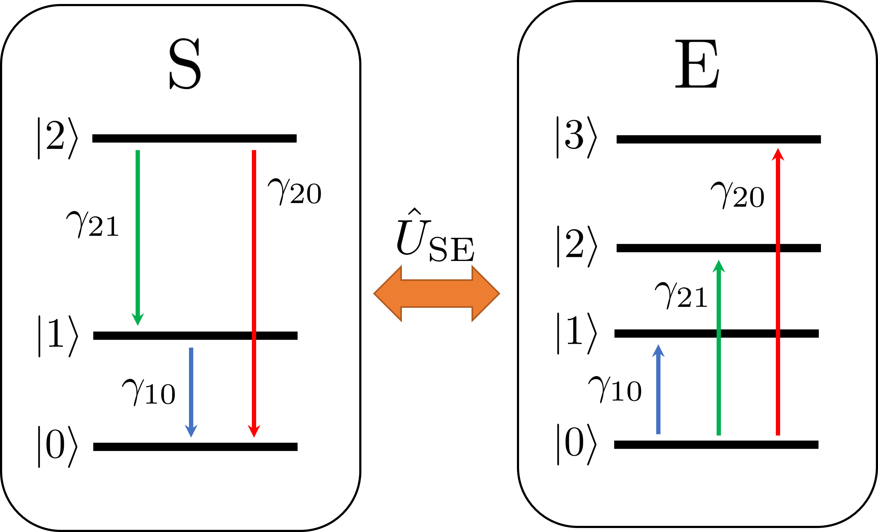
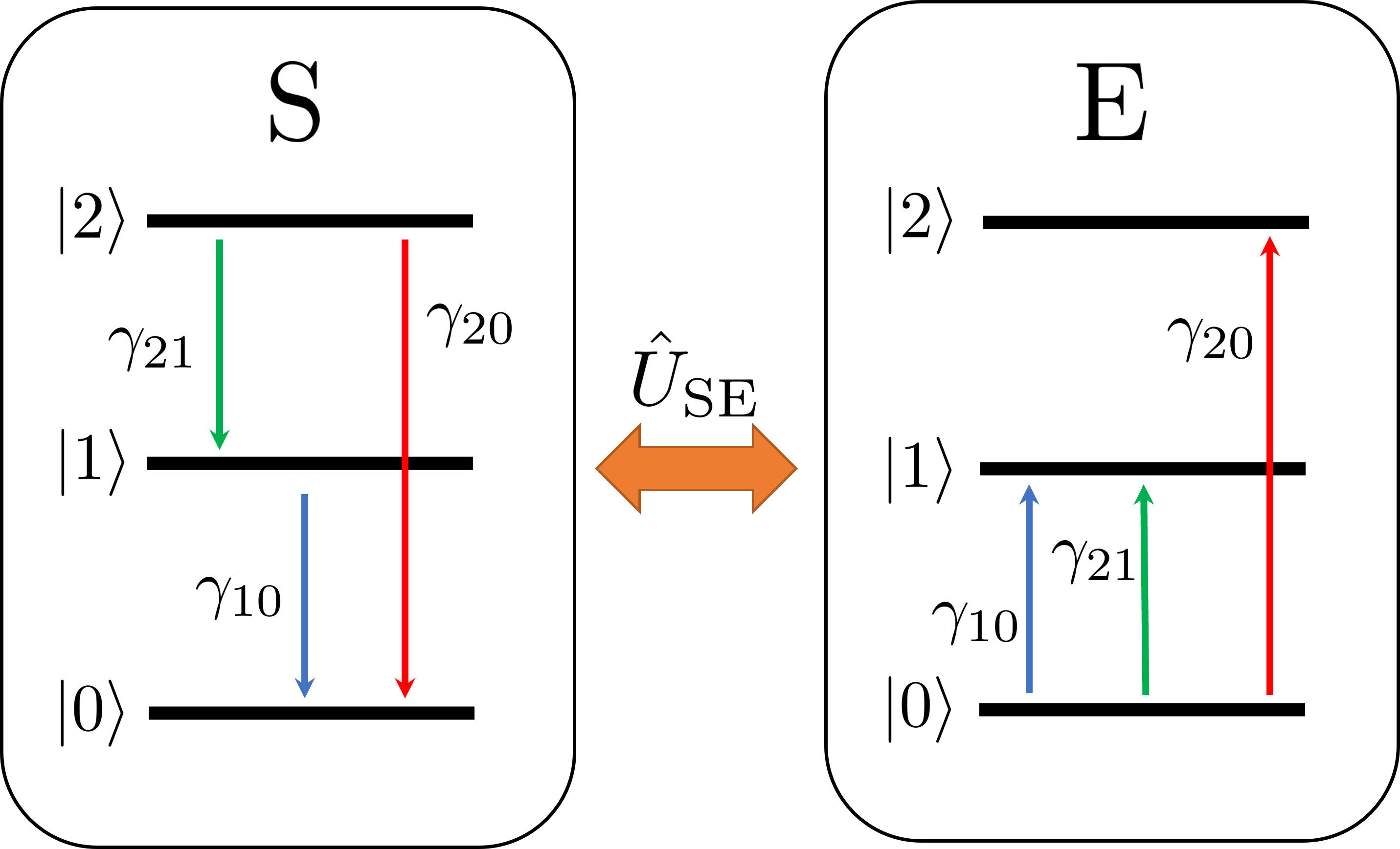
Specifically, given a generic density operator of S, we express its evolution under the action of as,
| (3) |
with being the ground state of the bath, the partial trace over the environment, and the unitary transformation that induces the mappings
| (4) |
In the above expression for and , kets describe a collection of vectors that are mutually orthogonal and orthogonal with as well. Since they represent the states where the environment stores the energy lost by S when moving from level to level , the construction in Eq. (4) implicitly assumes that the environment of the model is capable to discriminate among the different energy jumps. This condition is physically realized e.g. when the energy spectrum of S is composed by incommensurable levels. Notice also that this construction fixes the dimension of the Hilbert space of B, as well as the minimum number of Kraus operators needed to represent in the operator-sum representation [56] equal to , i.e.
| (5) |
with
| (6) |
By introducing ReMAD channels we now allow for the possibility that some of the transition events of S will excite the same internal degrees of freedom of the bath, a condition which can be achieved e.g. when the energy levels of the system are equally spaced, i.e. for all . In this case we can replace the unitary coupling in Eq. (4) with the new interaction
| (7) |
where are a (possibly energetically ordered) orthonormal basis of the environment E. The resulting LCPTP transformation is hence obtained by replacing Eqs. (3) and (5) with
| (8) |
where
| (9) |
is a Kraus set characterized by at most non-zero elements. It is easy to check that wile for , the ReMAD channel coincides with its corresponding MAD counterpart (indeed both reduce to the conventional qubit ADC). Also one can easily verify that for arbitrary , both and produce the same diagonal output states per diagonal input states , indeed
| (10) |
However for the two sets of transformations have rather different impact on the off-diagonal term of the input state. Consider for instance the qutrit () scenario where, thanks to the constraint (2) the transition matrix can be parametrized by 3 non-negative terms, e.g. , , and , forming a 3-dimensional vector spanning the domain
| (11) |
represented in Fig. 2 by the green rectangular right wedge delimited by the vertexes , , , , , and . In this case Eq. (7) reduces to
| (12) |
while, identifying the canonical basis states , , and with the column vectors , , and , we can express the associated Kraus operators in Eq. (9) as
| (13) |
Accordingly the action of on a generic density matrix of S produces the output state of the form
| (14) |
to be compared with the associated transformation induced by the MAD counterpart
| (15) |
with . As one can observe, while on the diagonal elements in both cases we have the usual decay of populations predicted by Eq. (10), the ReMAD output state in Eq. (14) exhibits a transfer of coherence that mixes the terms and which is not contemplated in the MAD output of Eq. (15). It is also worth noticing that in case either or the qutrit map and the qutrit map describe the same physical process.
As a final remark we notice that a particular example of ReMAD channel is provided by the so called beamsplitter type ADC introduced in Ref. [57]. This subclass of ReMAD channels describes the evolution of a qudit encoded in the first states of the Fock basis of an harmonic oscillator passing through a beamsplitter of transmittance . It’s straightforward to verify that such mappings are a special instance of the ReMAD class characterized by a transition matrix whose elements can be parametrized by the formula
| (16) |
so that . For this corresponds to having , , and : a plot of the parameter region spanned by beamsplitter type ADC for is reported in Fig. 2 .
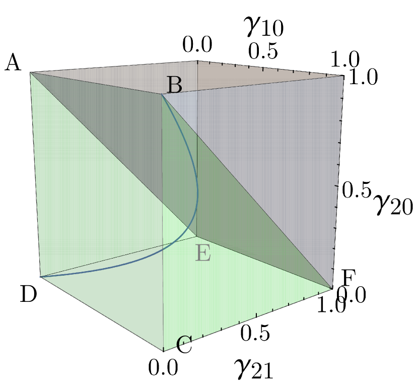
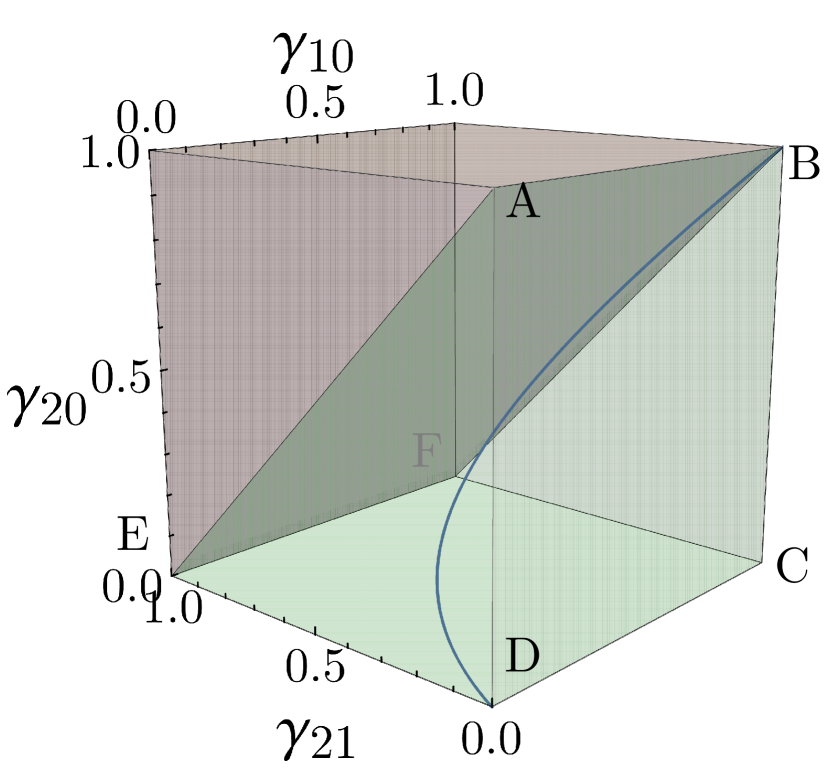
2.1 Complementary maps
At variance with what happens with MAD channels, the complementary map [13] of a generic ReMAD transformation is also a ReMAD channel (up to an isometry). This can be seen by recalling that can be obtained from Eq. (8) by replacing the partial trace over E with a partial trace over S, i.e.
| (17) |
where now are the operators
| (18) |
Notice next that up to an isometry mapping the energy levels of E into the corresponding levels of S (i.e. , ), has exactly the same form of the operators in Eq. (9) computed with a new lower-triangular transition matrix . The non-zero elements of , row by row, are obtained by a simple reordering of those of , i.e.
| (19) |
Specifically we can write
| (20) |
and hence
| (21) |
Again, as an example we provide the explicit form of the complementary channel of the qutrit ReMAD map of Eq. (14), i.e.
| (22) |
Notice finally that, as a consequence of Eq. (19), it follows that in the case of a beamsplitter type ADC defined by Eq. (16), one gets . This, thanks to Eq. (21), allows us to recover the well known fact that the complementary map of is isometrically equivalent to .
2.2 Composition rules
In Ref. [8] it was shown that MAD channels are closed under composition rules, a property that proves useful in studying their information capacities. In this section we investigate whether ReMAD channels behave similarly. Maybe surprisingly, it turns out that it’s not always the case. To begin with, let’s observe that from the composition rules of beamsplitters one can easily verify that the following identity holds true
| (23) |
(the symbol “” represents channel composition). Apart from this special case, the analysis is slightly convoluted. We therefore focus on the simplest, nontrivial case of qutrit systems defined by the input-output relations of Eq. (14). By explicit computation it follows that being and two transition matrices as in Eq. (1) we have
| (24) |
plus the Hermitian conjugate of off-diagonal elements. We are interested in understanding under which conditions a new transition matrix of elements exists such that
| (25) |
Among the equations above, those referring to elements 00, 02, 11, 12, 22 are all consistent with setting
| (26) |
(observe that such definitions are compatible with the request that , as well as with the normalization constraint for all ). Element 01 instead forces an additional constraint, i.e.
| (27) |
which is not necessarily granted. As a matter of fact by substituting in Eq. (27) the values for and obtained in Eq. (2.2) we get that in order to satisfy it we need
| (28) |
This identifies a specific region for the parameters and where the composition corresponds to a ReMAD channel. Notice in particular that, in agreement with Eq. (23), the identity in Eq. (28) is always fulfilled for beamsplitter type ADC, i.e. for and . Furthermore we observe that if is such that either or , then Eq. (28) is always satisfied for all the choices of . Of particular interest for our analysis is the first of these two configurations: here describes a ReMAD channel where the first two levels of S are untouched by the noise, while the third level gets mapped into the ground state with probability . Looking at Eq. (2.2) we notice that the transition probabilities and of the ReMAD channel , which emerge by the concatenation, coincide with those of (i.e. and ), while the transition probability increases with respect to . Specifically . Observing this, by varying , the last quantity can span over the entire interval . We can use this observation to claim that being and two qutrits ReMAD channels having the same transition probabilities connecting level 2 to level 1 and level 1 to level 0, but with larger than or equal to , then they can be connected via a third ReMAD channel as in Eq. (25).
2.3 Covariance
The ReMAD channels exhibit a covariance property under suitable unitary transformations. Specifically consider the set of unitary gates
| (29) | |||
| (30) |
with real. It then follows that
| (31) |
and similarly for the complementary channel we get
| (32) |
As we’ll see in the following the identities above turn out to be extremely useful in the computation of the capacities of our channels.
3 Review of quantum and private classical capacities
This section is dedicated to reviewing some basic notions about channel capacities for those readers who may be not familiar with these quantities. While the plethora of capacities for quantum channels includes a large collection of different functionals, our analysis will be focused on the quantum capacity and the private classical capacity .
3.1 Quantum Capacity and Private Classical Capacity
The quantum capacity of a quantum channel defines the maximum rate of transmitted quantum information achievable per channel use, assuming to act in the regime of i.i.d. noise [13, 14, 15, 16, 19, 17, 18, 20]. Intuitively it tells you how faithfully a quantum state, possibly correlated with an external system, can be sent and received by two communication parties if the communication line is noisy. Recently has also been showed to provide a lower bound to the space overhead necessary for fault tolerant quantum computation in presence of noise [58]. The formal definition of relies on the coherent information [59]. Assuming uses of the channel and a generic state we have
| (33) |
with the von Neumann entropy of the state , and the complementary channel of . Maximizing over we get the maximized coherent information for instances of the channel
| (34) |
and by regularization of this expression we get the maximized coherent information per channel use, that is the quantum capacity [60, 61, 62]
| (35) |
The private classical capacity quantifies the maximum rate of classical information achievable per channel use assuming also the privacy of communication (where privacy is intended as limiting to arbitrarily small the amount of information that an eavesdropper can extract from the environment during the communication). The fundamental tool needed to compute is the Holevo information functional [63]. Being an ensemble of quantum states , we have
| (36) |
Through the Holevo information we define next the private information for uses , that involves a maximization over all ensembles
| (37) |
from which finally can be computed via regularization over , i.e. [62, 64]:
| (38) |
We conclude our brief review by recalling that and obey data processing inequalities [14]. This means that, for (any) channel that can be expressed as a composition of other two LCPTP maps and (i.e. ) it follows
| (39) | |||
| (40) |
3.2 Degradability and antidegradability
The need of regularization in the evaluation of and poses a well known problem which ultimately is the underlying reason of our efforts here. An exception to this predicament is given by degradable [6] and antidegradable [29] channels, whose definitions and properties are reviewed here. A quantum channel is said degradable if a LCPTP map exists s.t.
| (41) |
while it’s said antidegradable if it exists a LCPTP map s.t.
| (42) |
In case is mathematically invertible, a simple direct way to determine whether it is degradable or not is to formally invert the composition in Eq. (41). This is done (if possible) by constructing the super-operator and by checking whether such object is LCPTP [65, 66]. The check can be performed by studying the positivity of its associated Choi matrix , i.e.
| (43) |
where given we set (see App. A for details). A completely similar argument can be made for antidegradability: in this case we can claim
| (44) |
where now is the Choi operator of the map .
As already mentioned the evaluation of the quantum a private classical capacity simplifies for degradable channels. To begin with, in this case and result to be additive, so the regularization over in Eq. (35) isn’t needed, leading to the single-letter formula [67]
| (45) |
Another important simplification arises from the fact that under degradability conditions the coherent information functional is concave w.r.t. the input state [68]. Accordingly if and turn out to be covariant under the action of some unitary group, the maximization in Eq. (45) can be further simplified. In the case of ReMAD channels where the properties (31) and (32) hold true, under degradability conditions we can write
| (46) | |||||
where in the last equality we made use of the invariance of von Neumann entropy under unitary transformations. Observing then that
| (47) |
we can conclude that for degradable ReMAD channels the maximization over of (45) can be restricted on the set of states which are diagonal in the canonical basis, i.e.
| (48) |
For antidegradable channels instead, due to a no-cloning argument [69], . Similarly, : the environment can reconstruct the channel output simply by applying the antidegrading channel, so no private information can be transmitted. Therefore for channels exhibiting antidegradability no maximizations are needed.
4 Degradability and antidegradability regions for ReMAD channels
In this section we study the degradability/antidegradability properties for qutrits ReMAD channels. Mimicking the approach used for other amplitude damping channels, we tackle the problem working under the heuristic assumption that if a degrading (or antidegrading) channel of a ReMAD channel exists, it is itself a ReMAD channel. While this choice is potentially suboptimal, numerical tests based on the more rigorous (but analytically impractical) matrix inversion method discussed in Sec. 3.2, reveals that this is not the case.
Reminding the isometric connection given in Eq. (21), we hence translate the degradability condition on into the problem of identifying a transition matrix s.t.
| (49) |
With a procedure similar to the one employed in Sec. 2.2 such equation can be mapped into the following constraints
| (50) |
which using the connection as in Eq. (19) to replace , , and , leads to
| (51) |
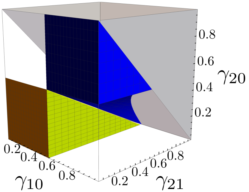
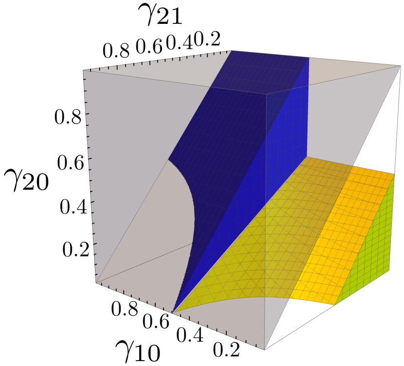
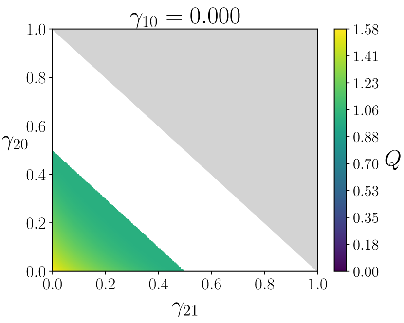
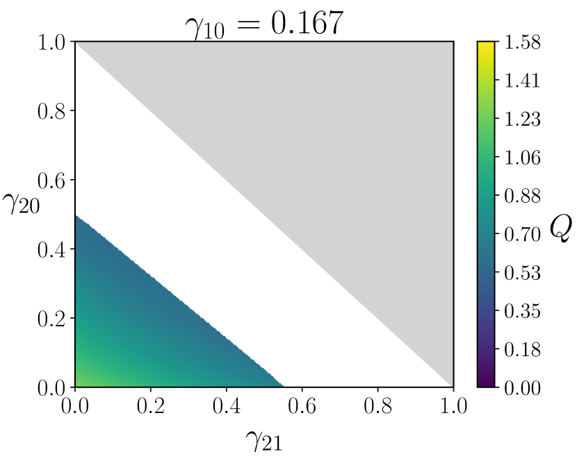
Imposing now the vector to belong to the domain of Eq. (11) we get the degradability region which we depict as the yellow region of Fig. 3. In such region we can compute exactly the value of and using the single-letter formula in Eq. (48) only involving diagonal input matrices. Results of such optimization are reported in Fig. 4 for different values of the parameters and . In the cases of and the obtained values were already known in the whole resulting parameter space (including some non-degradable regions), since there ReMAD channels reduce to double decay MAD channels, already studied in [8].
To check antidegradability of a ReMAD channel we follow the same path, looking for a that fulfills the identity
| (52) |
leading to a constraint that can be obtained from the one in Eq. (4) by exchanging with . This leads finally to
| (53) |
Imposing to have in brings us to the antidegradability region depicted in blue in Fig. 3.
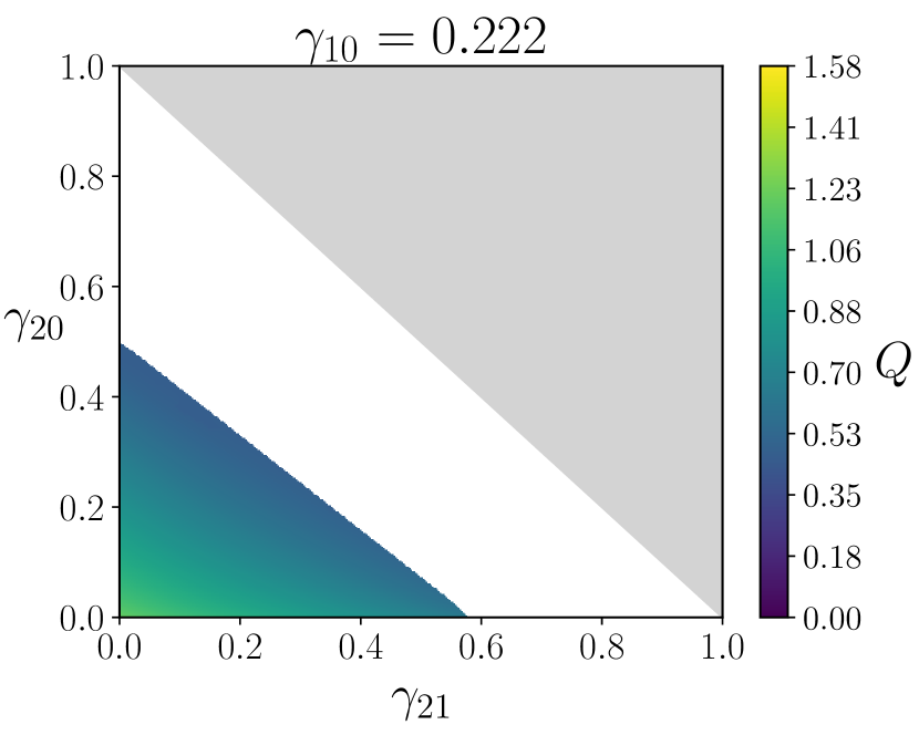
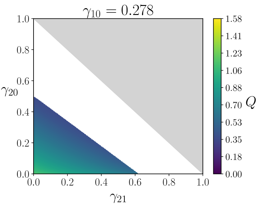
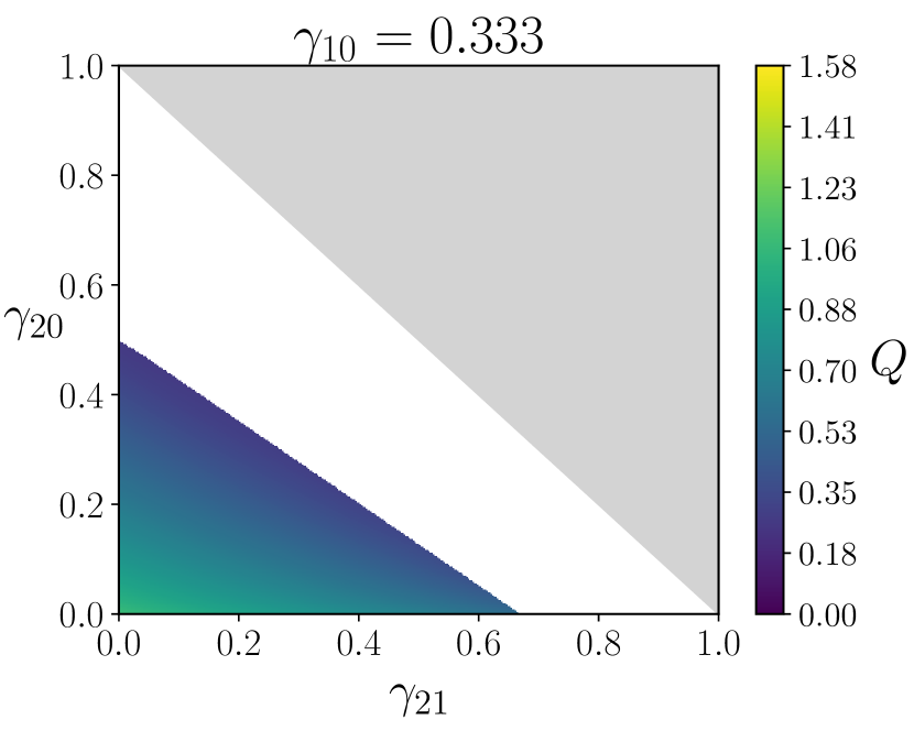
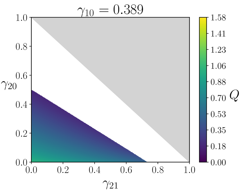
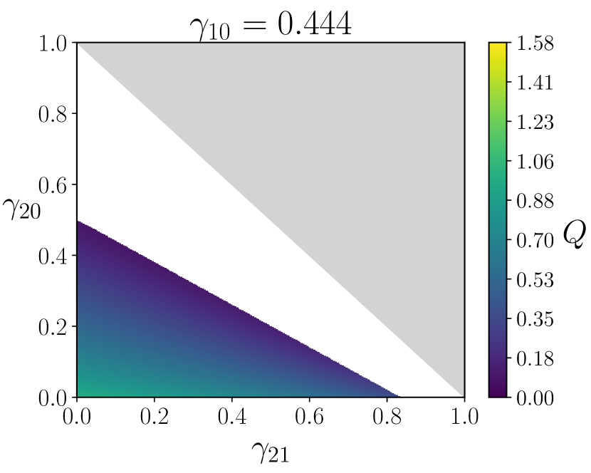
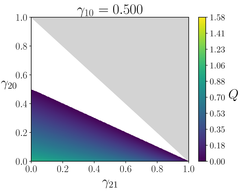
4.1 Capacities in non-degradable and non-antidegradable regions
In those regions of parameters for which degradability or antidegradability are not achieved a closed accessible expression for and is lacking. A notable exception is provided by the two planar regions identified respectively by (triangular surface of Fig. 2, identified by the vertexes ) and (rectangular region ). As one can observe from Fig. 3 they overlap only partially with the degradable and antidegradable regions: yet, thanks to the fact that there and coincide (see comments in Sec. 2), we can use the same techniques of [8], see Appendix C, to compute the quantum capacity of the associated ReMAD channels. Even for those points that aren’t explicitly degradable (or antidegradable), specifically:
- •
-
•
Planar region : here the channel is neither degradable nor antidegradable for all points which verify the conditions (right-lower quadrant in Fig. 5, right panel) or (left-upper quadrant in Fig. 5, right panel), see Appendix A.1. Applying techniques of [8], see Appendix C.2, we can conclude that in these regions the capacities assume symmetric values, i.e. give , we have
(55) with
(56) see right panel of Fig. 5. In the first expression the maximization is performed over the populations of the input state with respect to levels and under the consistency constraint ; the second identity instead follows from the observation that for fixed, the maximum of the r.h.s. term is always achieved by (no population assigned to the second excited level). Observe that the final expression in Eq. (61) exactly matches the quantum capacity of a qubit ADC channel with damping probability equal to [70].
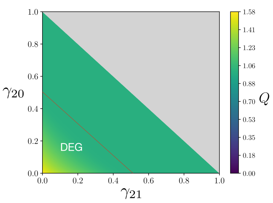
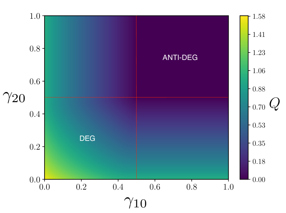
Figure 5: Left: (and ) for . The capacities are known also in the region that is not degradable nor antidegradable. Right: (and ) for . The capacities are known also in two regions that are not degradable nor antidegradable, see left-top panel () of Fig. 4 -
•
With a little additional effort we can also determine the exact value of for the elements on the boundary of the region identified by the constraints
(57) (notice that while for the points belong to the antidegradable region, for they are neither degradable nor antidegradable, see Appendix A.1). For these values Eq. (14) becomes
(58) which bears a close resemblance to the MAD channel with values , , i.e.
(59) for which capacities and have been computed for all values of [8], see Appendix C.3. The explicit connection between Eq. (58) and Eq. (59) follows by observing that, setting we can map the former into the latter via a unitary transformation on the input of the channel via the identity
(60) being the unitary operator reordering the canonical basis , , , into , , . Accordingly using Eq. (C.2) of Appendix C.2, in the region we can write
(61) in the region instead, as the channel is antidegradable. The overall profile of the capacities in this case reduces then to that of a qubit ADC with damping parameter [70]. We report its evaluation in Fig. 6, left panel. Notice that in the first expression the maximization is performed over the populations of the input state with respect to levels and under the consistency constraint . The second identity then follows by noticing that, similarly to what happens in Eq. (56), for fixed the maximum of the r.h.s. term is always achieved by (no population assigned to the first excited level). Comparing Eq. (61) with Eq. (55) we observe that on the edges and , that bound on the plane , the capacity of the channel takes the same values as those for fixed . Indeed we get
(62) which again is the capacity profile of a qubit ADC with damping parameter . See 6, right panel.
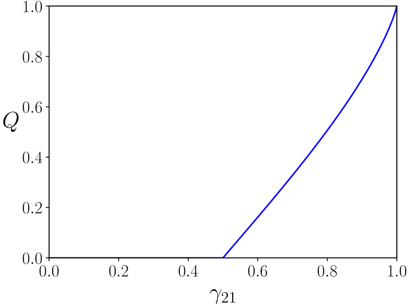
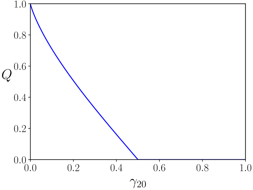
Figure 6: Left: as in Eq. (61), in the region the capacity is found for provably not degradable nor antidegradable channels. Right: as in Eq. (62), in the region the capacity is found for provably not degradable nor antidegradable channels. -
•
In the other sectors of the parameter space it is still possible to exploit some information theoretic properties to obtain computationally efficient upper bounds. For instance exploiting the considerations underlined in the final paragraphs of Sec. 2.2 and the data processing inequality (39) we can claim that, for fixed values of and , both and are non-increasing functions of , e.g.
(63)
5 Conclusions
We introduced and characterized a new class of physically relevant noise models for high-dimensional quantum systems. ReMAD channels enlarge the limited class of quantum channels for which an exact analytical or numerical approach in terms of quantum and private classical capacities is feasible. This has been shown by focusing on the simplest, yet nontrivial, case in which the system of interest is a qutrit. In such case we have shown the existence of a substantial region of the noise parameter space where the channels are degradable/antidegradable, allowing hence the direct expression of the associated quantum and private classical capacities. Also, by resorting to formal mapping to the case of MAD channels discussed in [8], we computed the value of these capacities in regions where is provably neither degradable nor antidegradable.
The full characterization in terms of information capacities, such as for instance classical capacity and two-way capacities, is still missing for ReMAD channels and will require further investigations. A semi-analytical treatment is instead achievable for the characterization of entanglement assisted quantum and classical capacities and of ReMAD channels, see Appendix B.
We acknowledge financial support by MIUR (Ministero dell’ Istruzione, dell’ Universitá e della Ricerca) by PRIN 2017 Taming complexity via Quantum Strategies: a Hybrid Integrated Photonic approach (QUSHIP) Id. 2017SRN- BRK, and via project PRO3 Quantum Pathfinder.
Appendix A Channel inversion
To compute we need to identify the inverse of the channel . Concretely the inversion of can be done by exploiting the fact that quantum channels are linear maps connecting vector spaces of linear operators. They can in turn be represented as matrices acting on vector spaces. This through the following “vectorization” isomorphism, also called Liouville representation:
where now is a matrix connecting and ( and being respectively the dimensions of and ). Given a Kraus set for , can be explicitly expressed as
| (65) |
Following Eq. (41) we have hence that for a degradable channel the following identity must apply
| (66) |
with the matrix representation of the LCPTP degrading channel , implying that the super-operator is now represented by
| (67) |
In the case of the qutrits ReMAD channel of (14), the inverse channel can also be expressed in the form
| (68) |
as one can check by direct computation.
A.1 Uniqueness of the degrading channel
In the most general case, even when the inverse of the channel considered exists, degrading maps may not be unique [71]. We show here how in the case of qutrit ReMAD channels, if these are degradable, the degrading channel must be unique and in the form of Eq. (67). For our analysis this is also equivalent to say that if the degrading channel can be found as in Eq. (67) but it’s not LCPTP, then the channel is not degradable. A proof of can be derived from [71, Theorem 3]:
Theorem 4 ([71]).
Let be a quantum channel and its complementary channel and let the corresponding super-operator of be full rank: . Then, if a degrading map exists, it is unique iff .
In our case and the ‘superoperator’ is always full rank except when or , since
is upper triangular and full rank, where we ordered the ‘basis’ as . So, whenever and we have that is full rank (hence invertible) and if doesn’t represent a LCPTP map then is not degradable.
Now the cases and remain, but it’s straightforward to show that these channels can’t degradable. Specifically we just need to show that , see [11, Sec. 2.1]. Looking at the expressions of the channels and their complementaries
| (72) | |||||
| (76) |
| (80) | |||
| (84) |
we see that the element and that the element . Therefore both cannot be degradable.
In synthesis, for ReMAD channels the degrading map can be uniquely found via the inverse matrix of the channel. If it doesn’t exist or the derived degrading map is not LCPTP then the channel is not degradable.
A similar analysis can be applied to antidegradability but typically we don’t need it in our discussion: where we can’t prove degradability, in those parameter regions we consider, ReMAD channels have positive capacity and hence cannot be antidegradable.
Appendix B Entanglement assisted quantum and classical capacities
The discovery of protocols such as quantum teleportation [72] and superdense coding [73] showed how entanglement could be leveraged as an additional resource in order to boost the communication performance between two communicating parties. The formalization of these entanglement-assisted protocols in Shannon-theoretic terms was given in [74, 75], where the entanglement-assisted classical capacity and entanglement-assisted quantum capacity were introduced. The peculiarity and the advantage with the definition of these capacities is that they are additive quantities and don’t need a regularization. Specifically, recalling the definition of the quantum mutual information
| (85) |
we have:
| (86) |
where the definition of is justified by the fact that in presence of entanglement a qudit quantum state can be teleported ‘spending’ two classical its (quantum teleportation) and viceversa two classical its can be communicated by sending a single qudit (superdense coding).
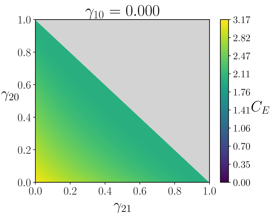
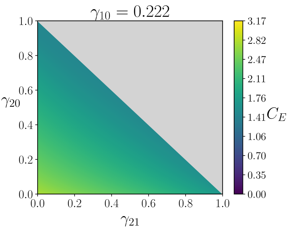
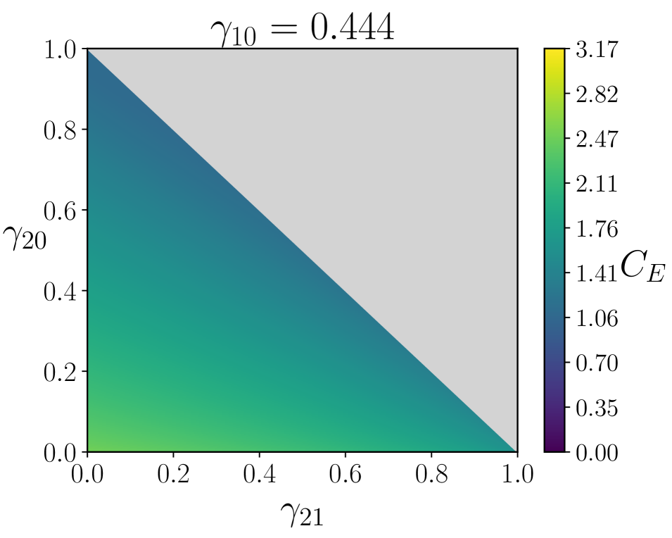
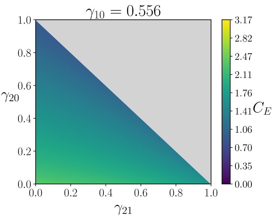
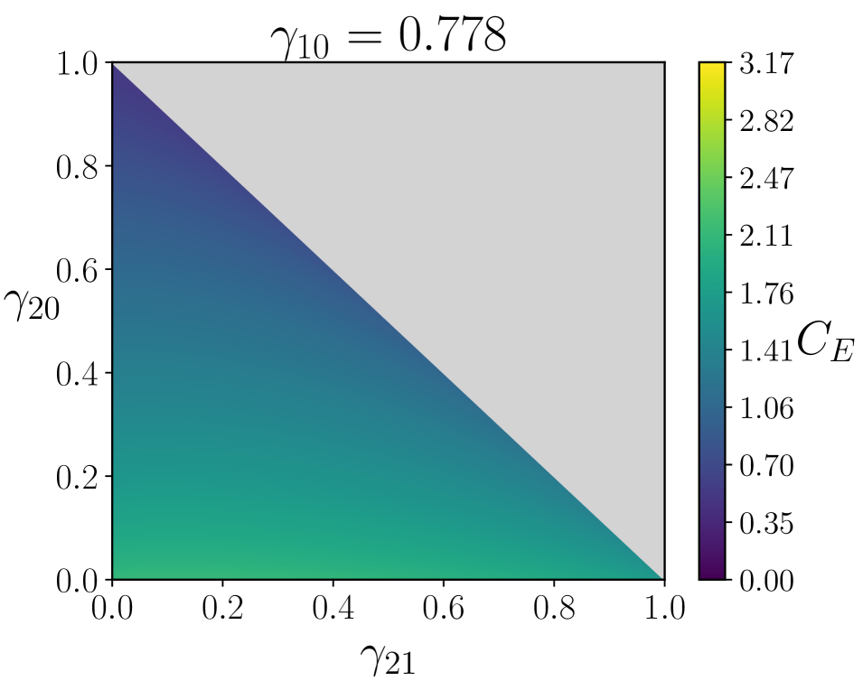
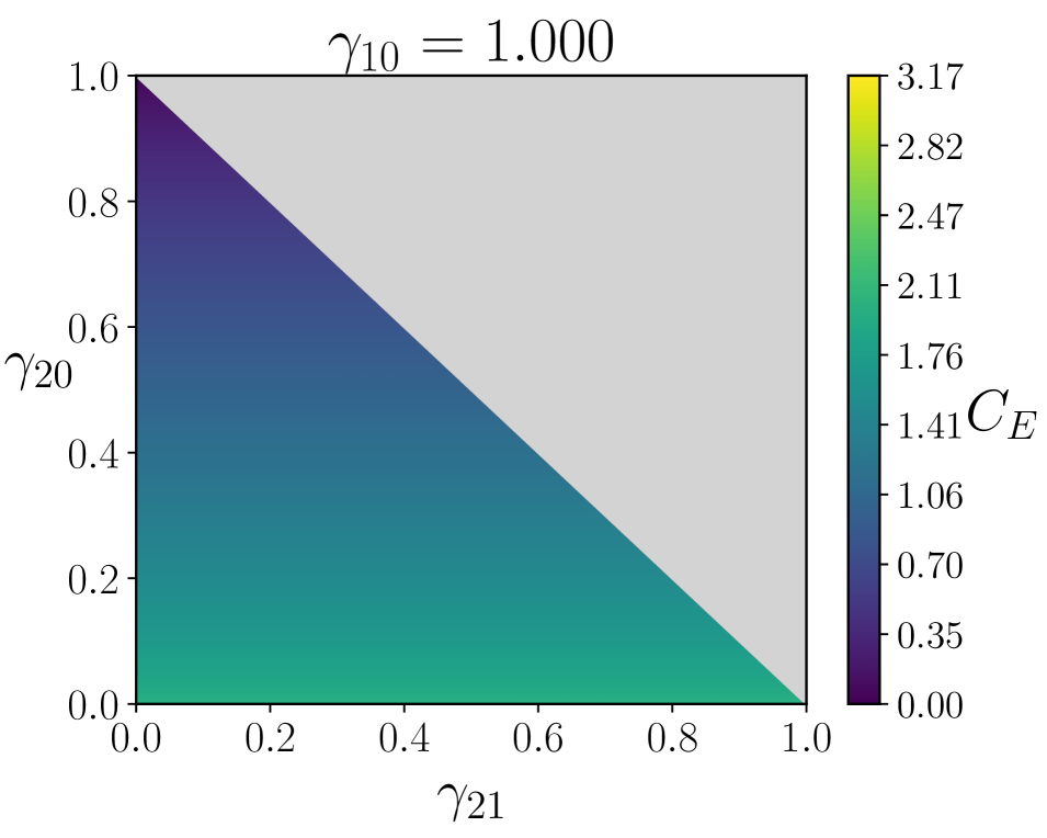
To effectively compute these quantities we notice that the Shannon entropy is always concave w.r.t. the input state but, as we saw before, the coherent information can be proved concave only when the channel is degradable. Nevertheless the quantum mutual information is always concave in the input state [14, chapter 13.4.2]. Therefore also can be maximized just over diagonal states if is a covariant channel by following steps as in Eq. (46). We report then in Fig. 7 the evaluation of for a qutrit ReMAD channel at varying and for some instances of values.
Appendix C and in non-degradable regions
C.1 and for
In case the actions of a generic qutrit ReMAD channel and of its complementary channel on a generic density matrix reduce to
| (87) | |||
| (91) |
It’s immediate to notice that has a noiseless subspace given by and consequently can establish the following lower bound:
| (92) |
This implies that can’t be antidegradable (we can reach the same conclusion by noticing that has a kernel that is not included into the kernel of [11]. For instance the former
contains while the latter doesn’t).
To compute the capacities we follow the channel inversion method described in Appendix A. We find that can be inverted when , and that is LCPTP when , identifying then the region of degradability for the channel. There, exploiting the channel covariance described in Sec. 2.3, we can compute and as (93)
We are therefore able to evaluate numerically the value of and on the boundary of the degradability region , where we are able to showing that there it’s equal to the lower bound in Eq. (92). This, together with the closure under composition of channels and data processing inequalities, allows us to conclude that in the entire parameter region .
C.2 and for
In the case of ReMAD channels with we have that channels and complementary channels actions reduce to
| (94) | |||
| (98) |
To compute the capacities we follow the channel inversion method described in Appendix A. We find that is invertible when , while is LCPTP when . From this follows that in this range of parameters the channels are degradable. Comparing Eqs. (94) with (98) we can also see that
| (99) |
Therefore, by the same argument above, we have that is antidegradable for and that for that range of values. To compute and in the degradable region we exploit the channels covariance described in Sec. 2.3 to maximize only over diagonal inputs, getting
| (100) |
The capacities are also known on the boundaries of the parameters space, since when one of the remaining damping parameters is 0 reduces to a single-decay qutrit MAD, for which and are known [8]. When one of the damping parameters is instead 1 we reduce to the MAD channel discussed in Appendix C.3, for which is already available. More precisely in Appendix. C.3 we compute , verifying that it coincides with the capacity of a qubit ADC.
Since the value of is known also on the boundaries of the degradable region, we can compare at and , for all . We find that the two are the same, i.e. , Accordingly, invoking the data-processing inequality and closure under composition, we can finally conclude that
| (101) |
that allows us to evaluate the and over the entire parameters region.
C.3 and for
We work here under the assumption of qutrit ReMAD channels with , for which the expression of channels and their complementary becomes
| (102) | |||
| (106) |
for such that . The channel cannot be degradable since has a kernel that is not included into the kernel of [11]. We are still able though to express exactly the value of its quantum capacity. Specifically we are able to state that
| (107) |
with defined as
| (108) | |||||
where we are able to restrict the maximization to diagonal density matrices of form of associated with the subspace . We plot in Fig. 8: we notice that when we have , coherently with the fact that in that parameter region the channel has zero capacity, i.e.
| (109) |
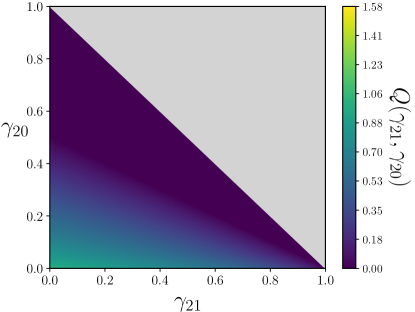
To prove Eq. (107) let us start by observing that provides a natural lower bound for and hence for :
We need now to show that can also upper bound . To do this we construct a new channel with larger capacity than , i.e.
| (110) | |||||
| (111) |
and for which we can show that
| (112) |
For this purpose notice that, since the population of level completely depleted, the output produced by can be reproduced by the channel operating on the two-levels Hilbert space , and producing qutrit states of A as outputs. In particular, calling a generic density matrix on we have
| (113) |
with associated complementary channel
| (114) |
where for we set .
fulfills the inequality (110) because , while producing the same output of , is also ‘wasting’ resources in the useless level . Explicitly, notice that we can write
| (115) |
being is the LCPTP map bringing the input state of the qutrit A to the qubit by transfer of the population of the level to followed by the erasure of , i.e.
| (116) |
where with . Equation (110) can then be derived as a consequence of the data processing inequality applied to (and ). The second part of the argument, i.e. Eq. (112), can instead be proved by noticing that, differently of the original channel that is not degradable, is degradable if
| (117) |
and antidegradable otherwise, i.e. for . This can be shown by observing that in the region identified by the inequality (117) the quantity
| (118) |
belongs to and can be used to build a single-decay qutrit MAD channel . Furthermore by direct calculation we get
| (119) |
which shows that acts as the degrading channel of . From Eqs. (113) and (114) it is also evident that can be recovered from by the substitution . Consequently, using the same construction of Eq. (119), we can conclude that is antidegradable when .
Finally, to derive Eq. (112) we observe that as the original channel also is covariant and accordingly we can express its capacity as
| (120) |
where the last identity follows from the fact that coincides with and by the fact that the positive component of the spectrum of coincides with the one of (strictly speaking the above derivation holds true only in the degradable region (117) of : still since nullifies for , we can apply (120) also in the antidegradability region of the channel where ).
Finally, we notice that for the effective channel in Eq. (113) can be replaced by the channel
| (121) |
mapping the two-level system into itself via a qubit ADC with damping parameter . Accordingly, following the same analysis done above it follows that and coincide with the respective capacities of a qubit ADC, computed in Ref. [70].
References
- Cozzolino et al. [2019] D. Cozzolino, B. Da Lio, D. Bacco, and L. K. Oxenløwe, Advanced Quantum Technologies 2, 1900038 (2019), URL https://doi.org/10.1002/qute.201900038.
- Wang et al. [2020] Y. Wang, Z. Hu, B. C. Sanders, and S. Kais, Frontiers in Physics 8, 479 (2020), ISSN 2296-424X, URL https://doi.org/10.3389/fphy.2020.589504.
- Hill [2021] A. Hill, Beyond qubits: Unlocking the third state in quantum processors (2021), URL https://medium.com/rigetti/beyond-qubits-unlocking-the-third-state-in-quantum-processors-12d2f84133c4.
- Fanizza et al. [2020] M. Fanizza, F. Kianvash, and V. Giovannetti, Phys. Rev. Lett. 125, 020503 (2020), URL https://doi.org/10.1103/PhysRevLett.125.020503.
- Kianvash et al. [2022] F. Kianvash, M. Fanizza, and V. Giovannetti, Quantum 6, 647 (2022), ISSN 2521-327X, URL https://doi.org/10.22331/q-2022-02-09-647.
- Devetak and Shor [2005] I. Devetak and P. W. Shor, Communications in Mathematical Physics 256, 287 (2005), URL https://doi.org/10.1007/s00220-005-1317-6.
- D'Arrigo et al. [2007] A. D'Arrigo, G. Benenti, and G. Falci, New Journal of Physics 9, 310 (2007), URL https://doi.org/10.1088/1367-2630/9/9/310.
- Chessa and Giovannetti [2021a] S. Chessa and V. Giovannetti, Communications Physics 4, 22 (2021a), ISSN 2399-3650, URL https://doi.org/10.1038/s42005-021-00524-4.
- Chessa and Giovannetti [2021b] S. Chessa and V. Giovannetti, Quantum 5, 504 (2021b), ISSN 2521-327X, URL https://doi.org/10.22331/q-2021-07-15-504.
- Leditzky et al. [2022] F. Leditzky, D. Leung, V. Siddhu, G. Smith, and J. Smolin, The platypus of the quantum channel zoo (2022), arXiv:2202.08380, URL https://doi.org/10.48550/arXiv.2202.08380.
- Cubitt et al. [2008] T. S. Cubitt, M. B. Ruskai, and G. Smith, Journal of Mathematical Physics 49, 102104 (2008), URL https://doi.org/10.1063/1.2953685.
- Singh and Datta [2022] S. Singh and N. Datta, npj Quantum Information 8, 50 (2022), ISSN 2056-6387, URL https://doi.org/10.1038/s41534-022-00550-2.
- Holevo [2019] A. S. Holevo, Quantum Systems, Channels, Information (De Gruyter, 2019), URL https://doi.org/10.1515/9783110642490.
- Wilde [2017] M. M. Wilde, Quantum Information Theory (Cambridge University Press, Cambridge, 2017), 2nd ed., ISBN 9781107176164, URL https://doi.org/10.1017/9781316809976.
- Watrous [2018] J. Watrous, The Theory of Quantum Information (Cambridge University Press, Cambridge, 2018), ISBN 9781107180567, URL https://doi.org/10.1017/9781316848142.
- Hayashi [2017] M. Hayashi, Quantum information theory (Springer, 2017), 2nd ed., ISBN 9783662497234, URL https://doi.org/10.1007/978-3-662-49725-8.
- Nielsen and Chuang [2010] M. A. Nielsen and I. L. Chuang, Quantum Computation and Quantum Information: 10th Anniversary Edition (Cambridge University Press, Cambridge, 2010), ISBN 9781107002173, URL https://doi.org/10.1017/CBO9780511976667.
- Imre and Gyongyosi [2012] S. Imre and L. Gyongyosi, Advanced Quantum Communications: An Engineering Approach (Wiley-IEEE Press, 2012), 1st ed., ISBN 1118002369, URL https://doi.org/10.1002/9781118337462.
- Holevo and Giovannetti [2012] A. S. Holevo and V. Giovannetti, Reports on Progress in Physics 75, 046001 (2012), URL https://doi.org/10.1088/0034-4885/75/4/046001.
- Gyongyosi et al. [2018] L. Gyongyosi, S. Imre, and H. V. Nguyen, IEEE Communications Surveys Tutorials 20, 1149 (2018), URL https://doi.org/10.1109/COMST.2017.2786748.
- Huang [2014] Y. Huang, New Journal of Physics 16, 033027 (2014), URL https://doi.org/10.1088/1367-2630/16/3/033027.
- Cubitt et al. [2015] T. Cubitt, D. Elkouss, W. Matthews, M. Ozols, D. Pérez-García, and S. Strelchuk, Nature Communications 6, 6739 (2015), ISSN 2041-1723, URL https://doi.org/10.1038/ncomms7739.
- Elkouss and Pérez-García [2018] D. Elkouss and D. Pérez-García, Nature Communications 9, 1149 (2018), ISSN 2041-1723, URL https://doi.org/10.1038/s41467-018-03428-0.
- Hastings [2009] M. B. Hastings, Nature Physics 5, 255 (2009), ISSN 1745-2481, URL https://doi.org/10.1038/nphys1224.
- Smith and Yard [2008] G. Smith and J. Yard, Science 321, 1812 (2008), URL https://doi.org/10.1126/science.1162242.
- Li et al. [2009] K. Li, A. Winter, X. Zou, and G. Guo, Phys. Rev. Lett. 103, 120501 (2009), URL https://doi.org/10.1103/PhysRevLett.103.120501.
- Zhu et al. [2019] E. Y. Zhu, Q. Zhuang, M.-H. Hsieh, and P. W. Shor, IEEE Transactions on Information Theory 65, 3973 (2019), URL https://doi.org/10.1109/TIT.2018.2889082.
- Zhu et al. [2017] E. Y. Zhu, Q. Zhuang, and P. W. Shor, Phys. Rev. Lett. 119, 040503 (2017), URL https://doi.org/10.1103/PhysRevLett.119.040503.
- Caruso and Giovannetti [2006] F. Caruso and V. Giovannetti, Phys. Rev. A 74, 062307 (2006), URL https://doi.org/10.1103/PhysRevA.74.062307.
- Smith and Smolin [2008] G. Smith and J. A. Smolin, in 2008 IEEE Information Theory Workshop (2008), pp. 368–372, URL https://doi.org/10.1109/ITW.2008.4578688.
- Brádler et al. [2010] K. Brádler, N. Dutil, P. Hayden, and A. Muhammad, Journal of Mathematical Physics 51, 072201 (2010), URL https://doi.org/10.1063/1.3449555.
- Watanabe [2012] S. Watanabe, Phys. Rev. A 85, 012326 (2012), URL https://doi.org/10.1103/PhysRevA.85.012326.
- Gyongyosi [2014] L. Gyongyosi, IEEE Access 2, 333 (2014), URL https://doi.org/10.1109/ACCESS.2014.2317652.
- Sutter et al. [2017] D. Sutter, V. B. Scholz, A. Winter, and R. Renner, IEEE Transactions on Information Theory 63, 7832 (2017), URL https://doi.org/10.1109/TIT.2017.2754268.
- Pirandola et al. [2017] S. Pirandola, R. Laurenza, C. Ottaviani, and L. Banchi, Nature Communications 8, 15043 (2017), ISSN 2041-1723, URL https://doi.org/10.1038/ncomms15043.
- Anshu [2017] A. Anshu, in 2017 IEEE Information Theory Workshop (ITW) (2017), pp. 214–218, URL https://doi.org/10.1109/ITW.2017.8277947.
- Leditzky et al. [2018] F. Leditzky, D. Leung, and G. Smith, Phys. Rev. Lett. 120, 160503 (2018), URL https://doi.org/10.1103/PhysRevLett.120.160503.
- Tomamichel et al. [2017] M. Tomamichel, M. M. Wilde, and A. Winter, IEEE Transactions on Information Theory 63, 715 (2017), URL https://doi.org/10.1109/TIT.2016.2615847.
- Wilde et al. [2017] M. M. Wilde, M. Tomamichel, and M. Berta, IEEE Transactions on Information Theory 63, 1792 (2017), URL https://doi.org/10.1109/TIT.2017.2648825.
- Christandl and Müller-Hermes [2017] M. Christandl and A. Müller-Hermes, Communications in Mathematical Physics 353, 821 (2017), ISSN 1432-0916, URL https://doi.org/10.1007/s00220-017-2885-y.
- Wang et al. [2019] X. Wang, K. Fang, and R. Duan, IEEE Transactions on Information Theory 65, 2583 (2019), URL https://doi.org/10.1109/TIT.2018.2874031.
- Hirche et al. [2022] C. Hirche, C. Rouzé, and D. Stilck França, Quantum 6, 862 (2022), ISSN 2521-327X, URL https://doi.org/10.22331/q-2022-11-28-862.
- Fang and Fawzi [2021] K. Fang and H. Fawzi, Communications in Mathematical Physics 384, 1615 (2021), ISSN 1432-0916, URL https://doi.org/10.1007/s00220-021-04064-4.
- Hirche and Leditzky [2022] C. Hirche and F. Leditzky, Bounding quantum capacities via partial orders and complementarity (2022), arXiv:2202.11688, URL https://doi.org/10.48550/arXiv.2202.11688.
- Fawzi et al. [2021] O. Fawzi, A. Shayeghi, and H. Ta, in 2021 IEEE International Symposium on Information Theory (ISIT) (2021), pp. 272–277, URL https://doi.org/10.1109/ISIT45174.2021.9517913.
- Hammerer et al. [2010] K. Hammerer, A. S. Sørensen, and E. S. Polzik, Rev. Mod. Phys. 82, 1041 (2010), URL https://doi.org/10.1103/RevModPhys.82.1041.
- Sangouard et al. [2011] N. Sangouard, C. Simon, H. de Riedmatten, and N. Gisin, Rev. Mod. Phys. 83, 33 (2011), URL https://doi.org/10.1103/RevModPhys.83.33.
- Reiserer and Rempe [2015] A. Reiserer and G. Rempe, Rev. Mod. Phys. 87, 1379 (2015), URL https://doi.org/10.1103/RevModPhys.87.1379.
- Damask [2005] J. N. Damask, Polarization optics in telecommunications (Springer Series in Optical Sciences, 2005), 1st ed., ISBN 978-0-387-26302-1, URL https://doi.org/10.1007/b137386.
- Gottesman et al. [2001] D. Gottesman, A. Kitaev, and J. Preskill, Phys. Rev. A 64, 012310 (2001), URL https://doi.org/10.1103/PhysRevA.64.012310.
- Bartlett et al. [2002] S. D. Bartlett, H. de Guise, and B. C. Sanders, Phys. Rev. A 65, 052316 (2002), URL https://doi.org/10.1103/PhysRevA.65.052316.
- Terhal et al. [2020] B. M. Terhal, J. Conrad, and C. Vuillot, Quantum Science and Technology 5, 043001 (2020), URL https://doi.org/10.1088/2058-9565/ab98a5.
- Cai et al. [2021] W. Cai, Y. Ma, W. Wang, C.-L. Zou, and L. Sun, Fundamental Research 1, 50 (2021), ISSN 2667-3258, URL https://doi.org/10.1016/j.fmre.2020.12.006.
- Carretta et al. [2021] S. Carretta, D. Zueco, A. Chiesa, Á. Gómez-León, and F. Luis, Applied Physics Letters 118, 240501 (2021), URL https://doi.org/10.1063/5.0053378.
- Stinespring [1955] W. F. Stinespring, Proceedings of the American Mathematical Society 6, 211 (1955), URL https://doi.org/10.2307/2032342.
- Kraus [1971] K. Kraus, Annals of Physics 64, 311 (1971), ISSN 0003-4916, URL https://doi.org/10.1016/0003-4916(71)90108-4.
- Ouyang [2014] Y. Ouyang, Quantum Information and Computation 14, 917 (2014), URL https://doi.org/10.26421/QIC14.11-12-2.
- Fawzi et al. [2022] O. Fawzi, A. Müller-Hermes, and A. Shayeghi, in 13th Innovations in Theoretical Computer Science Conference (ITCS 2022), edited by M. Braverman (Schloss Dagstuhl – Leibniz-Zentrum für Informatik, Dagstuhl, Germany, 2022), vol. 215 of Leibniz International Proceedings in Informatics (LIPIcs), pp. 68:1–68:20, ISBN 978-3-95977-217-4, ISSN 1868-8969, URL https://doi.org/10.4230/LIPIcs.ITCS.2022.68.
- Schumacher and Nielsen [1996] B. Schumacher and M. A. Nielsen, Phys. Rev. A 54, 2629 (1996), URL https://doi.org/10.1103/PhysRevA.54.2629.
- Lloyd [1997] S. Lloyd, Phys. Rev. A 55, 1613 (1997), URL https://doi.org/10.1103/PhysRevA.55.1613.
- Shor [2002] P. W. Shor, in Lecture notes, MSRI Workshop on Quantum Computation (Quantum Information and Cryptography) (2002), URL https://www.msri.org/workshops/203/schedules/1181.
- Devetak [2005] I. Devetak, IEEE Transactions on Information Theory 51, 44 (2005), URL https://doi.org/10.1109/TIT.2004.839515.
- Holevo [1973] A. S. Holevo, Problemy Peredachi Informatsii 9, 3 (1973), URL http://www.mathnet.ru/eng/ppi903.
- Cai et al. [2004] N. Cai, A. Winter, and R. W. Yeung, Problems of Information Transmission 40, 318 (2004), URL https://doi.org/10.1007/s11122-005-0002-x.
- Wolf and Perez-Garcia [2007] M. M. Wolf and D. Perez-Garcia, Physical Review A 75, 012303 (2007), URL https://doi.org/10.1103/PhysRevA.75.012303.
- Smith and Smolin [2007] G. Smith and J. A. Smolin, Physical review letters 98, 030501 (2007), URL https://doi.org/10.1103/PhysRevLett.98.030501.
- Smith [2008] G. Smith, Physical Review A 78, 022306 (2008), URL https://doi.org/10.1103/PhysRevA.78.022306.
- Yard et al. [2008] J. Yard, P. Hayden, and I. Devetak, IEEE Transactions on Information Theory 54, 3091 (2008), URL https://doi.org/10.1109/TIT.2008.924665.
- Bennett et al. [1997] C. H. Bennett, D. P. DiVincenzo, and J. A. Smolin, Phys. Rev. Lett. 78, 3217 (1997), URL https://doi.org/10.1103/PhysRevLett.78.3217.
- Giovannetti and Fazio [2005] V. Giovannetti and R. Fazio, Phys. Rev. A 71, 032314 (2005), URL https://doi.org/10.1103/PhysRevA.71.032314.
- Brádler [2015] K. Brádler, Open Systems & Information Dynamics 22, 1550026 (2015), URL https://doi.org/10.1142/S1230161215500262.
- Bennett et al. [1993] C. H. Bennett, G. Brassard, C. Crépeau, R. Jozsa, A. Peres, and W. K. Wootters, Phys. Rev. Lett. 70, 1895 (1993), URL https://doi.org/10.1103/PhysRevLett.70.1895.
- Bennett and Wiesner [1992] C. H. Bennett and S. J. Wiesner, Phys. Rev. Lett. 69, 2881 (1992), URL https://doi.org/10.1103/PhysRevLett.69.2881.
- Bennett et al. [1999] C. H. Bennett, P. W. Shor, J. A. Smolin, and A. V. Thapliyal, Phys. Rev. Lett. 83, 3081 (1999), URL https://doi.org/10.1103/PhysRevLett.83.3081.
- Bennett et al. [2002] C. Bennett, P. Shor, J. Smolin, and A. Thapliyal, IEEE Transactions on Information Theory 48, 2637 (2002), URL https://doi.org/10.1109/TIT.2002.802612.
