A density-matrix renormalization group algorithm for simulating quantum circuits with a finite fidelity
Abstract
We develop a density-matrix renormalization group (DMRG) algorithm for the simulation of quantum circuits. This algorithm can be seen as the extension of time-dependent DMRG from the usual situation of hermitian Hamiltonian matrices to quantum circuits defined by unitary matrices. For small circuit depths, the technique is exact and equivalent to other matrix product state (MPS) based techniques. For larger depths, it becomes approximate in exchange for an exponential speed up in computational time. Like an actual quantum computer, the quality of the DMRG results is characterized by a finite fidelity. However, unlike a quantum computer, the fidelity depends strongly on the quantum circuit considered. For the most difficult possible circuit for this technique, the so-called “quantum supremacy” benchmark of Google Inc. Arute et al. (2019), we find that the DMRG algorithm can generate bit strings of the same quality as the seminal Google experiment on a single computing core. For a more structured circuit used for combinatorial optimization (Quantum Approximate Optimization Algorithm or QAOA), we find a drastic improvement of the DMRG results with error rates dropping by a factor of compared with random quantum circuits. Our results suggest that the current bottleneck of quantum computers is their fidelities rather than the number of qubits.
I Introduction
Quantum computers and the quantum many-body problem are intimately connected. On the one hand, a quantum computer is essentially an instance of the quantum many-body problem on which one has a high level of control. On the other hand, the most promising applications that are foreseen for quantum computers correspond to solving other instances of the quantum many-body problem such as calculating the properties of new materials Bauer et al. (2020), of new molecules for medicine, or of new catalysts for important chemical reactions Reiher et al. (2017).
A common misconception of the field of quantum computing is that all quantum many-body problems are exponentially difficult to solve by classical computers because the size of the Hilbert space grows exponentially as when the system size increases. This supposedly dooms many-body simulations on classical computers to failure, and therefore calls for computers with quantum physics inside. This “large Hilbert space fallacy” is however contradicted by the success of classical many-body methods for tackling many of these hard problems. At heart, these methods use the fact that physical problems are structured. Physicists take advantage of the separation of time, energy or length scales, of statistical (mean field) behavior, or of symmetries, to design methods to solve seemingly exponentially hard problems. Even for genuine strongly correlated systems, there exist very powerful many-body techniques that can solve them in a variety of situations, taking advantage of an underlying feature. Without these features—namely had the physical world been a random point in the Hilbert space—there would indeed be nothing to understand and the problem would be exponentially difficult. However, since the physical world actually makes sense, one can argue that simulating a many-body physical problem is not as hopeless as one could naively think.
The subject of this article is to discuss the problem of simulability in the context of quantum computers that use quantum circuits, that is discrete sequences of quantum gates. This questioning is at the core of the possibility for a “quantum advantage”, for if a quantum computer can be easily simulated, one might as well use the (classical) simulator instead of developing a genuine quantum computer. The quantum circuit model of quantum computing ignores many structures of the underlying many-body problem. For instance, it does not contain the basic concepts of space, time or energy. Nor does it contain the concept of fermionic or bosonic statistics nor the representation of symmetries (spin, relativity). As a result, it might seem that such a quantum computer must be much harder to simulate than a physics-based many-body problem. An extreme version of a quantum circuit designed to be as featureless as possible is the seminal “quantum supremacy experiment” Arute et al. (2019) of Google Inc. Google initially claimed that simulating their supremacy experiment would require 10,000 years on the largest existing supercomputer. Subsequent studies (that we shall review in Section II) Gray and Kourtis (2021); Pan and Zhang (2021); Pan et al. (2022) showed that this initial surmise was exaggerated and that the task could be executed in a few hundred seconds. This progress in classical simulations could be obtained through a precise analysis of the structure of the quantum circuit. Yet, the computational cost of these simulations remains exponential in the number of qubits.
In this article, we use a different class of algorithms, borrowed from quantum many-body theory, whose complexity increases only as a power of , making the simulation of hundreds of qubits possible. This exponential gain in computational complexity is obtained in exchange for a quantum state compression that implies a finite fidelity of the calculation. In this sense, these algorithms share some characteristics with actual quantum computers, which also suffer from a finite fidelity. A first step in that direction was taken in Zhou et al. (2020), where some of us developed a quantum circuit version of the time-evolving bond decimation Daley et al. (2004); Vidal (2004); White and Feiguin (2004) (TEBD) algorithm. It was found that surprisingly good fidelities could be obained at a relatively low computational cost. Here, we develop a generalization of the density-matrix renormalization group White (1993); Schollwöck (2011) (DMRG) algorithm to quantum circuits. Although technically more complex, DMRG allows one to improve on the TEBD algorithm in a systematic way.
We benchmark our quantum-circuit-DMRG algorithm on three different quantum circuits: The “quantum supremacy” sequence of Arute et al. (2019)—optimized to be as difficult to simulate as possible, another slightly easier random circuit and a “useful” circuit used in the Quantum Approximate Optimization Algorithm (QAOA) Edward et al. (2014) for combinatorial optimization. We find that even with the most difficult “quantum supremacy” sequence, DMRG can produce bitstrings that have the same quality as the one demonstrated in Arute et al. (2019) on a single computing core. More importantly, we find that for the QAOA sequence, we reach a fidelity per gate much higher than the one found in the Sycamore processor. Our numerical experiments provide important benchmarks of the fidelities that can be reached on a classical computer, and therefore of what the quantum hardware must fulfill to claim genuine quantum supremacy or advantage. Since our DMRG algorithm scales only polynomially with , it implies that quantum computers must improve their fidelities to access regimes that cannot be simulated.
This article is organized as follows: in section II, we review the current status of quantum supremacy and of quantum circuit simulation techniques. Section III contains a summary of the main findings of this article. The DMRG technique is developed in section IV. Section V showcases how DMRG works in practice and discusses some implementation details. Section VI discusses in which regime the DMRG algorithm provides an optimum solution. Section VII shows the relation between the fidelity and the cross-entropy benchmarking obtained in our simulations. Finally, we conclude in section VIII. This articles relies heavily on tensor network techniques. Appendix A contains a short self-contained introduction to tensor networks for readers unfamiliar with these techniques.
II A critical review of quantum supremacy
Almost three years ago, the annoucement by Google of having reached the milestone of “quantum supremacy” dazzled both the academic community and the general public Arute et al. (2019). Google managed to control transmon qubits and to perform a circuit comprising two-qubit gates. They obtained a quantum state that had a small (), yet measurable overlap with the ideal state that they were supposed to get. While this state did not permit any useful computation, Google surmised that producing something similar using classical simulations would be prohibitive (10,000 years on the largest supercomputer) and hence claimed to have reached quantum supremacy.
Since Ref. Arute et al. (2019), another group has produced an almost identical experiment using a very similar technology Wu et al. (2021). There has also been other claims of quantum supremacy, most notably using “boson sampling” Zhong et al. (2020). Here, we shall not discuss these more recent claims for two reasons. First, the hardness of these tasks is strongly debated Popova and Rubtsov (2021); Villalonga et al. (2021); Oh et al. (2022). Second, and more importantly: while the Google experiment represents a milestone on the path towards building a quantum computer, these most recent claims corresponds to very specific tasks and the devices are not programmable.
Here, we review the status of the classical simulation challenges to these “quantum supremacy” claims, namely we review the various works that have attempted to simulate the experiments in a reasonable classical computing time Gray and Kourtis (2021); Pan and Zhang (2021); Pan et al. (2022); Yong et al. . In particular, we shall try to explain in simple terms why the initial claim of “10,000 years” was challenged a few days later to be only two days and why it has eventually been shown that a simulation of quantum supremacy could be performed in a few hundred seconds.
II.1 An exponentially difficult experiment
A quantum computer with qubits has an internal state that can be written as
| (1) |
where , ,, correspond to the different qubits. The vector , whose components are the complex numbers , can be considered as a large vector of dimension . One initializes the state in (typically all qubits in state , i.e. ) and then applies a sequence of unitary gates. Formally, these gates transform the state of the quantum computer into
| (2) |
where the are unitary matrices (two-qubit gates or combination thereof). A direct simulation of Eq. (2) by a series of (sparse) matrix-vector multiplications is referred to as a “Schrödinger approach”. In an experiment, however, one does not have access to the many-qubit wavefunction. Instead, one measures the different qubits and obtains a bitstring with probability .
In Ref. Arute et al. (2019), the authors used qubits and a highly unstructured set of two-qubit gates spread over layers. The experiment was repeated times to produce a sequence of bitstrings . Since the quantum sequence was highly unstructured, the distribution was expected to be fairly chaotic so that all bitstrings would have a probability to be obtained of order , i.e. the experiment essentially outputs random bitstrings. Ref. Arute et al. (2019) is primarily a global system validation experiment. The authors performed exact numerical simulations of Eq. (2) to obtain the exact distribution that should have been obtained from the experiment. By estimating how the perfect distribution correlates with the distribution obtained experimentally, one is able to assert to which degree the quantum computer has performed the requested task. The metric used to analyse this correlation is the “cross-entropy benchmarking”
| (3) |
which can be estimated experimentally as
| (4) |
It is expected theoretically, and observed experimentally, that due to decoherence and imprecisions in the gates and measurements, the cross-entropy benchmarking shall decay exponentially:
| (5) |
with an error rate . Ref. Arute et al. (2019) was able to verify Eq. (5) with an error . For the largest depth where the exact distribution was too computationally costly to be calculated, they extrapolated that . The “quantum supremacy” claim was that obtaining a set of bitstrings with the same fidelity by simulations would require 10,000 years on the largest supercomputer.
It should be noted that this experiment is exponentially difficult. Indeed, in order for the set of bitstrings to be distinguishable from just plain random bitstrings distributed uniformly, one needs the statistical error in the estimation of Eq. (4) to be smaller than what is estimated, i.e. . Since the statistical error decreases as , it implies an exponentially large number of samples,
| (6) |
Ref. Arute et al. (2019) pushed the quantum chip to the extreme limit where there remained just enough fidelity for the signal to be measured. For instance going to would have implied an increase of the measurement time by a factor . The authors also had to give up a little on the universality or programmability of the chip to maintain a low enough error rate : they chose, for each pair of qubit, the two-qubit gate that had the best fidelity by optimizing the microwave pulses. Subsequent experiments that used the same chip but focused on “useful” quantum circuits used only 10-20 qubits to retain accurate enough results Arute et al. (2020).
II.2 Exchanging a smaller memory footprint for an exponential increase of computational time
Immediately following Google’s supremacy claim, a team from IBM proposed an algorithm that, according to their estimation, would require only days to complete the supremacy task instead of years Pednault et al. (2019). Such a speed up (a factor ) begs for an explanation. A direct naive “Schrödinger” evaluation of Eq. (2) would require of the order of floating operations by holding the vector in memory and applying the two-qubit gates one by one. Such an algorithm would require operations. Hence, since large supercomputers can perform more than floating operations per second, the supremacy task could, according to this naive estimation, be performed in at most a few minutes, not thousands of years. This however requires one to hold a vector of size in memory, i.e. TBytes of RAM which is more than what supercomputers have (typically by more than a factor 10). To get around this difficulty, one designs algorithms that require exponentially more operations in exchange for a smaller memory footprint.
To illustrate how the tradeoff between memory footprint and computational time can be implemented in practice, imagine that we group the qubits into 2 groups of and qubits (). A first index labels the first group and a second index labels the second group . An arbitrary gate has matrix elements . Such a tensor can be considered as a matrix where the two indices are considered as a meta-index that index the lines and the two other indices index the columns. Using singular value decomposition, such a matrix can be factorized into a sum of terms of the form
| (7) |
where and act separately on the first and second group of qubits, respectively (see Appendix A for details on the SVD operation). Since the wave function initially factorizes, , one can rewrite Eq. (2) as,
| (8) |
with
| (9) | |||||
| (10) |
Now, we need only to perform matrix vector products of much smaller sizes, and . In return for this much smaller memory footprint, and depend explicitly on . One has to repeat the calculation for each to perform the sum, which has an exponential computational cost . Simulations that use Eqs. (8,9,10) are known as ”Schrödinger-Feynman” simulations. In a Schrödinger-Feynman simulation, the only problematic gates are the two-qubit gates that couple the two groups. These gates have (Control-NOT or Control-Z) or at most (arbitrary two-qubit gates). For all the gates that do not couple the two groups of qubits, and there is no increase of computational time. Another aspect is that one can calculate the amplitude for as many configurations as needed with no additional cost except for the one of storing these amplitudes in memory. The initial statement of Google of 10,000 years was associated with an estimation of the computational cost of a Schrödinger-Feynman simulation. We see that this computational estimation is strongly tied to the available memory. More memory would allow one to perform an optimized splitting of the qubits into two groups or no splitting at all, resulting in a much smaller computational cost. The IBM proposal Pednault et al. (2019), which was not implemented, was to take advantage of the hard drives of the supercomputer as temporary storage so that the full qubit wave-function could be held in memory, thereby considerably reducing the computational time. The drawback of this approach, besides the obvious difficulty of performing an actual implementation, is the fact that adding just one extra qubit would require a doubling of the memory footprint hence making the simulation out of reach.
II.3 The hierarchy of “open” versus “closed” versus “weak” simulations
The final blow on the supremacy claim came from a combination of works Refs Gray and Kourtis, 2021; Pan and Zhang, 2021; Pan et al., 2022; Yong et al., , in which the authors found a route to perform the simulation of the “quantum supremacy” experiment in a few hundred of seconds and demonstrated that the solution could be implemented in an actual very large supercomputer. This series of works essentially closed the gap between the simulations and the experiments. This corresponds to a drop by a factor with respect to the initial estimate of 10,000 years. This new gain comes from the combination of two new ingredients.
The first important point is that there are several simulation modes of decreasing power. The Schrödinger (Schrödinger-Feynman) simulation provides the full -qubit wavefunction (as many amplitudes as one can store). We refer to this simulation mode as “open” in the sense that they do not target a specific bitstring . Open simulations produce much more information than what the experiment outputs. Another simulation mode, that we refer to as a “closed” simulation, targets a single bitstring and computes the amplitude
| (11) |
Closed simulations are generically much easier than open ones. A last type of simulation, “weak” simulations, would produce the same output as an actual quantum computer, namely random bitstrings distributed according to the probability . There exists a clear hierarchy between these different simulation modes: an open simulation provides more information than a closed one which in turn provides more information than a weak simulation (or an actual quantum computer). One of the key steps in speeding up our simulations was to go from the open mode to the closed one.
The fact that closed simulations are superior to weak ones is not totally obvious. It follows from a simple algorithm recently proposed in Ref. Bravyi et al. (2021) that allows one to sample from the calculation of a polynomial number of individual amplitudes at smaller depth . The algorithm of Ref. Bravyi et al. (2021) constructs a bitstring iteratively, starting from the initial bitstring and taking into account the two-qubit gates one by one. is identical to except for the two qubits that are affected by the two-qubit gate. There are only four such bitstrings . One computes the four probabilities and samples from this conditional distribution, i.e. with probability . It is straightfoward to verify that this scheme indeed provides a bitstring distributed according to . Note that in the context of the supremacy experiment where all have similar orders of magnitude, this algorithm is not necessary and a simple Metropolis-Hastings sampling could be used instead (see the discussion in Appendix C).
II.4 Optimized contraction strategies of tensor networks
In the closed simulation mode, the challenge of the calculation lies in the summation over all the internal indices of the tensors in Eq. (11). Finding the optimum order for these summation is a hard (NP complete) problem, but there exist good heuristic algorithms for finding close to optimum contraction strategies Gray and Kourtis (2021). These optimum orders are in general very different from a simple summation from right to left, i.e. from the contraction done in a Schrödinger or Schrödinger-Feynman simulation. The memory/CPU tradeoff is implemented using a “slicing” approach: one carefully selects a few indices that are frozen in order to lower the cost of contracting the tensor network. The different values taken by these indices (the equivalent of the in the Schrödinger-Feynman simulations) are distributed over different computing nodes or GPU cards as these tasks are embarrassingly parallel. For the reader not familiar with the concept of tensor contractions and slicing, a small introduction is given in appendix A.
Using these techniques (i.e. closed simulations and good contraction strategies), the authors in Ref. Gray and Kourtis (2021) estimated that the time to compute a single amplitude on a graphics card (GPU) could be reduced down to years with perfect fidelity. The same authors estimated that it would take days to match the supremacy experiment, i.e. produce one million samples with the cross-entropy benchmarking fidelity. To arrive at this estimate, they took advantage of (i) the computing ressources of the large supercomputer “Summit”, (ii) the fact that the computing time to compute a few amplitudes that differ only by the value of a few qubits is not significantly higher than computing a single amplitude and (iii) that a fidelity of can be obtained by mixing a few () high amplitude (large ) samples with bitstrings sampled from a uniform random distribution.
A few months later, the estimated time to sample one million bitstrings with fidelity was further reduced to days Huang et al. (2020), based on similar ideas and refinements by a team at Alibaba. These authors estimated the time to compute one perfect sample on Summit to seconds. Like the previously mentioned study Gray and Kourtis (2021), they proposed to sample Sycamore by computing batches of amplitudes at no significant cost increase in a partly “closed”, partly “open” mode.
The approach was further optimized by Pan and Zhang Pan and Zhang (2021) in the so-called “big-batch method” that optimized the choice of the qubits left in open mode. They managed to compute two million bitstrings with a large cross-entropy benchmarking in 5 days on a small cluster of 60 GPUs Pan and Zhang (2021). However these bitstrings had many qubits in common, hence were strongly correlated. In a second study Pan et al. (2022), they have proposed a new ”sparse state method” that lowers the contraction cost of the supremacy circuit tensor network by cleverly introducing a few errors at specific locations. They have produced independent batches of correlated bitstrings in hours on a cluster of GPUs, and via importance sampling finally obtained one million uncorrelated samples with fidelity. In the same work, they estimated that the sampling time for Sycamore could be reduced to a few dozen of seconds on a large supercomputer.
Ref. Yong et al. produced two million correlated bitstrings from Sycamore with cross-entropy benchmarking fidelity in seconds. This calculation was performed on the Sunway TaihuLight supercomputer with 42 million effective cores, with an algorithm inspired by the work of Pan and Zhang (2021), and taking advantage of a new heuristic for slicing and contraction path optimization. It demonstrated that the parallelization of these algorithms could be effectively implemented on a very large supercomputer. Together Ref.Pan et al. (2022) and Ref.Yong et al. convincingly show that a supercomputer can match the Sycamore chip, even for a task whose only interest lies in having been optimized to be difficult to simulate.
Hence, the initial claim of “quantum supremacy” has been, to a large extent, deflated. However, the classical simulations reviewed above required colossal resources to achieve this goal. Since the problem is exponentially hard, a marginal improvement of the qubit fidelity (which would allow the experiment to go to larger depth) would have made the problem inaccessible to simulations. A second aspect is that problems that are impossible to simulate are easy to find, and the quantum supremacy experiment is to a large extent an artificial problem constructed for the sole purpose of being difficult to simulate. The question remains of what the quantum supremacy experiment taught us in terms of where one stands in the route to building genuine quantum computing capabilities for useful problems. In this article, we also use tensor network simulations to benchmark the performance of quantum computers. However, our focus is very different from the above high-performance computing calculations. While previous simulations are essentially exact with a small linear speed-up coming from the finite targeted fidelity, we borrow quantum state compression techniques from many-body theory that exchange a finite fidelity for an exponential gain in computing time. As we shall see, these complementary techniques provide strong insights in the influence of a finite fidelity on computing capabilities and what it would take for a quantum computer to reach a regime that is both interesting and out of reach of simulations.
III Summary of the main results
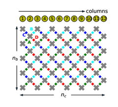
In this article, we develop an approximate DMRG algorithm for the simulation of quantum circuits. Before going into the mathematical details of how the technique works, we report on the results of our simulations for a few relevant circuits. Denoting by the perfect state that one should obtain and by the actual approximate state obtained in the simulation, the main quantity of interest in this article is the fidelity of the simulation, defined as
| (12) |
Since decreases exponentially with the number of two-qubit gates () in these simulations, we define the error rate per two-qubit gate as
| (13) |
This quantity can be directly compared to experiments. For instance, assuming , then the of the quantum supremacy experiment translates into an error per two-qubit gate, for each of the two-qubit gates. This effective value accounts for the actual two-qubit gate errors (around ), the one-qubit gate errors (around ) and the measurement errors (around ).
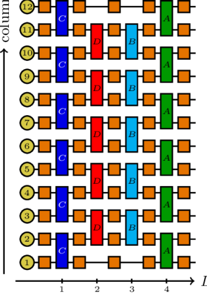
We perform most of our simulations on a qubit system very close to the -qubit Sycamore chip of Ref. Arute et al., 2019, see Fig. 1. All the simulations presented here have been performed with limited computational ressources: one to few computing processes (fewer than 12) that have lasted at most a few hours. We will consider three different quantum circuits.
Sequence I is essentially the quantum supremacy sequence of Google. layers are applied. For each layer, one applies a random one-qubit gate on each qubit, followed by the so-called fsim gate on all pairs of qubits according to the pattern ABCD-CDBA-ABCD-… (see Fig. 1). Sequence I has been designed to entangle the qubits as quickly as possible and therefore be as hard to simulate as possible.
Sequence II is identical to sequence I but with a pattern rotated by 90 degrees, i.e. the sequence is CDBA-BACD-CDBA…
Sequence III is, in contrast to sequence I and II, designed to perform a supposedly useful task. It implements the Quantum Approximate Optimization Algorithm (QAOA). QAOA is attracting a lot of attraction as a candidate algorithm to solve combinatorial optimization problems on a (noisy) quantum computer Harrigan et al. (2021). It can be viewed as a discrete variational version of the adiabatic quantum computing paradigm.
Our main findings are summarized in the next three subsections.
III.1 Simulating the supremacy sequence
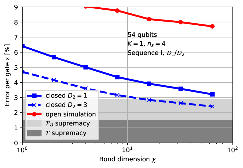
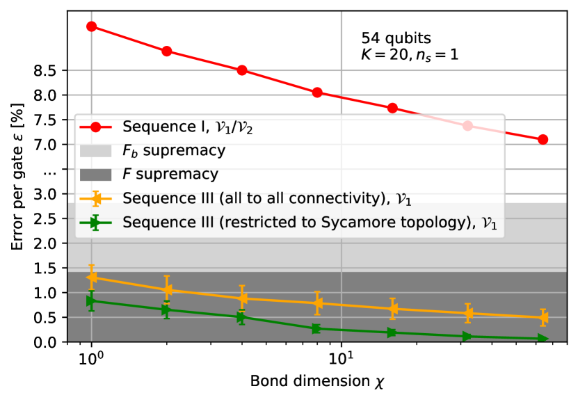
Fig 2(a) shows the error obtained in our simulations for the quantum supremacy sequence I with a system of qubits. The -axis is the “bond dimension” that controls the level of compression of the quantum state, hence the accuracy. The computational cost of the simulation scales polynomially as with a memory footprint . An exact simulation would correspond, at large depth, to an exponentially large , but we are here very far from this regime.
The red curve shows the results in the “open” mode. We find that the error rate for the largest studied is fairly high, around , much higher than in state-of-the-art experiments. Going to “closed” mode provides an important gain in error rate, typically by more than a factor two with our technique, enabling one to reach . By optimizing the closed mode (curve , the details of the closed mode will be explained later), one reaches at a computational cost that is still moderate.
To compare this error rate with the experimental one, we need to know the error rate associated with the experimentally measured cross-entropy benchmarking, i.e. , not . The authors of Ref. Arute et al. (2019) have argued that for their experiment for large enough depths. While this statement can be proven for certain classes of noise, it is not universal. For instance, it cannot hold at small depth since while . Nor does it hold for systems consisting of disjoint pieces, for which fidelity composes multiplicatively while composes additively when small Gao et al. (2021).
For our simulation technique, a very different relation holds:
| (14) |
We shall provide strong evidence, both numerical and analytical, to support Eq. (14). It follows that the obtained in our simulations corresponds to (light gray zone). Hence the bitstrings provided by these simulations have a higher cross-entropy benchmarking fidelity than those provided by Ref. Arute et al. (2019) and in that sense, our technique can be considered as another breach in the claim of quantum supremacy. Note that since the relation between and is highly non-universal, the fact that Eq. (14) holds in our simulation does not imply a similar relation in the experiments.
III.2 Scaling with the number of qubits
A very important difference between the present work and previous attempts at bridging the quantum supremacy gap is the scaling of the simulations with the number of qubits. Indeed, in our simulations, the exponential difficulty lies in increasing the fidelity, not the number of qubits.
In our present implementation, the computational cost of a simulation scales as , where is the number of qubits in the first column and the number of columns (see Fig. 1). The memory required scales as . The parameter depends on the precise mode of calculation. Algorithms using Projected Entangled Pair States (PEPS) should provide a computational cost linear in both and Pang et al. (2020); Lin et al. (2021).
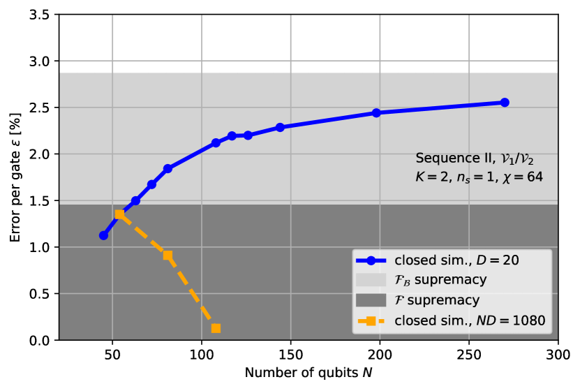
The scaling with is illustrated in Fig. 2(c), where we show a calculation as a function of (by varying ) at fixed for sequence II. We perform simulations with more than qubits, while the error shows a limited increase before saturating (see the discussion in Zhou et al. (2020)). Such simulations would be totally out of the scope of standard simulation approaches. We emphasize again that the experiment corresponding to the blue curve in Fig. 2(c) would be exponentially difficult: one cannot increase at fixed experimentally (even assuming that so many qubits would be available) because the cross-entropy benchmarking would become too small to be measurable in a reasonable time. Working at fixed experimental measurement time, i.e. fixed or equivalently keeping the product constant corresponds to the orange curve in Fig. 2(c). We see here a first difference of behavior between our compression algorithms and actual experiments: our error rate actually drastically drops with in the orange curve, as our algorithm becomes essentially exact at small depth. This indicates that in order to beat compression algorithms, quantum hardware must improve in fidelity and/or connectivity: a mere increase of the number of qubit is not sufficient.
III.3 Influence of the quantum circuit on the fidelity
A second important difference between actual experiments and our compression algorithm appears upon considering different quantum circuits. One of the chief results of Arute et al. (2019) is that the fidelity of the experiment depends only on the number and type of gates applied and should to a large extent be agnostic to the type of circuit ran. In practice, however, random circuits such as sequence I or II are experimentally easier than more structured circuits. This is due to several factors: these random circuits are optimally parallel without any idle time that could lead to further decoherence; there is a compensation of errors due the random choice of gates; and in the case of Ref. Arute et al. (2019), a pair-by-pair optimization of the fidelity of the two-qubit gates that could not have been performed had these gates corresponded to the prescription of an algorithm. This increased difficulty—for experimental hardware—of running structured circuits is well known in the field of quantum benchmarking, see e.g Proctor et al. (2022).
In our compression algorithm, we find, in sharp contrast with the above observations, that more structured quantum circuits are much easier to compress than random ones. While this result is not surprising on a qualitative level, the magnitude of the improvement in error rate that we observe is very high, with an error rate for open simulation dropping by a factor from for random circuits down to for QAOA circuits with the same and .
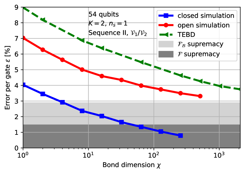
Fig. 2(b) shows a result for sequence II, which is only a slight modification of sequence I. We observe that this slight modification of the sequence provides a twofold gain in , bringing the open simulation almost down to the gray region and the closed simulations deep into the dark gray region. Fig. 2(b) also shows the result of the TEBD algorithm of Ref. Zhou et al., 2020 (green curve), showing that the DMRG algorithm presented in this article is a clear improvement over TEBD.
Fig. 2(d) contrasts the results between sequence I and the QAOA sequence III. The results for the QAOA sequence correspond to the same number of qubits and same two-qubit gate count , i.e. such that experimentally one would expect a fidelity lower than the observed for sequence I, for the reasons mentioned above. In contrast, the results of the compression algorithm are drastically better for sequence III than for sequence I. Two plots are presented in Fig. 2(d). In the orange curve, we have simulated the QAOA sequence supposing that the chip had perfect connectivity (a two-qubit gate can be applied between any pair of qubits). We find that the error rate in an open simulation is reduced by a factor compared to sequence I, with at . The green curve corresponds to a circuit that respects the nearest-neighbor topology of the Sycamore chip. This topology puts additional constraints on the graphs that can be optimized with a given “budget” of two-qubit gates. It results in simpler graphs being simulated, and a further drop of the error rate down to for in the hardest open simulation mode. We note that two recent works Dupont et al. (2022); Sreedhar et al. (2022) considered a related problem (performance of a TEBD approach similar to Zhou et al. (2020) for a QAOA optimization) and arrived to conclusions that are, at least qualitatively, consistent with ours. The simulation of QAOA circuits with up to 54 qubits was also tackled in a recent work Medvidović and Carleo (2021) using an alternative representation of the quantum state based on neural networks, the Restricted Boltzmann Machine Jónsson et al. (2018), with similar conclusions.
While it is difficult to draw general conclusions from specific experiments, we conjecture that “useful” quantum circuits, structured by nature, are generically much easier to simulate than random ones. It follows that in order for a quantum computer to show a genuine quantum advantage (i.e. quantum supremacy but for a useful task), far better fidelities will need to be demonstrated by the hardware.
IV A Density-Matrix Renormalization Group algorithm for simulating quantum circuits

We now describe the quantum state compression algorithm used in this article. This algorithm is inspired by the Density-Matrix Renormalization Group (DMRG) algorithm that has been highly instrumental for solving 1D quantum many-body problems White (1992); Schollwöck (2011). Our algorithm can be considered as a “unitary” version of the original “Hermitian” DMRG algorithm.
Our method combines a Schrödinger-type of simulation with compression steps where we approximate the quantum state with a Matrix Product State ansatz. This compression is performed every few layers of gates and requires one to find optimum contraction strategies for small tensor networks. The main new ingredient of this algorithm is the compression step. We emphasize that, although we introduce it in the context of Schrödinger-type of simulations, this step is in fact very general and could in principle be combined with other tensor-network simulations approaches.
Since this article relies heavily on the tensor networks naturally associated to quantum circuits, the reader not familiar with these concepts may read the short introduction in Appendix A.
IV.1 The Matrix Product State ansatz
An arbitrary state with qubits
| (15) |
is described by a very large tensor . A matrix product state (MPS) factorizes and compresses this tensor by writing it as a product of tensors contracted in a chain-like geometry. See Fig. 3 for a schematic. Each tensor contains the information on qubits:
| (16) | |||||
The “virtual” indices take at most values, where is known as the bond dimension. If is exponentially large, then a MPS can in fact describe any quantum state. Here, however, we restrict ourselves to rather small values of , in which case the MPS can only be an approximation of the entangled state that one aims at describing. There exists an important literature on many-body problems that can be successfully addressed by MPS variational ansatz Schollwöck (2011). The unentangled initial product state is naturally a MPS with .
Note that in contrast to the approach of Ref. Zhou et al. (2020), grouping the qubits is not, in principle, necessary: one could use instead the conventional grouping and larger values of to obtain a variational ansatz as expressive as the one used with our non trivial grouping . We found however that, in practice, some groupings can be advantageous for some circuits, e.g. in the case where some qubits inside one group are highly entangled. Since the first and last tensors only have virtual index instead of , it is computationally advantageous to have more qubits in the corresponding groups.
IV.2 The main building block of the algorithm: the compression step
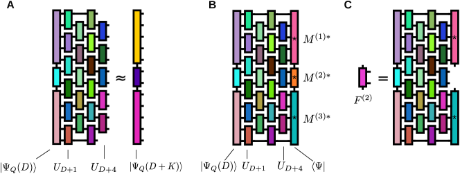
The central part of the algorithm performs the following task: One starts from a MPS , supposedly a good approximation of the exact state . The problem is to find the best MPS that approximates the state after one has applied layers of gates of the circuit, as illustrated on Fig. 4A. Namely, we want to determine
| (17) |
To perform this optimization, we optimize one given tensor of at a time while the remaining tensors are kept fixed. This optimization can be performed exactly using the simple formula Eq. (20) derived below. It amounts to the contraction of a small tensor network. To obtain the global optimum, we sweep over the choice of the tensor as in the single-site DMRG algorithm. Typically, a small number of sweeps is needed to obtained convergence towards . Note that we have also tried variants of this algorithm analogous to original two-site DMRG algorithm (where two consecutive tensors are optimized simultaneously) but did not observe any significant improvement with respect to the simpler single-site version.
IV.2.1 Optimization of a single tensor
Once we fix all the tensors of the MPS except for the tensor , the scalar product to be optimized takes the form
| (18) |
where the trace means summation over all indices. Very importantly, this scalar product is a linear function of . The tensor network for the left-hand side of Eq. (18) is shown in Fig. 4B. It follows that is defined by the contraction of the tensor network shown in Fig. 4C. In other words, simply corresponds to the tensor network for the full scalar product to which the tensor has been removed. Note that in Fig. 4C, the two tensors on the right (corresponding to ) are complex conjugated.
Before doing the optimization, we need to enforce the fact that the MPS is a normalized state, i.e. . This is best done by performing a series of factorizations on the tensors for to bring the MPS in the so-called “orthogonal form”, see Schollwöck (2011). In this form, the norm of the MPS is simply given by
| (19) |
Introducing the Lagrange multiplier , the optimization over with the constraint boils down to maximizing the function
i.e. we are maximizing a simple quadratic form. The optimum tensor is easily found, and is related to the “fitting” approach used in the MPS literature Saberi et al. (2009); Stoudenmire and White (2010). It reads
| (20) |
with . Eq. (20) is the central equation around which all this article is constructed. In addition, using Eqs (18), (20), one finds that the scalar is also the partial fidelity of the calculation
| (21) |
which allows one to keep track of the progress of the optimization inside a sweep over or over different sweeps.
For each calculation of , one obtains the local maximum of the partial fidelity with respect to , hence can only increase as we sweep over the different tensors . We can then repeat the sweep over all tensors several times, yielding monotonically increasing fidelities . The final value that we obtain after several sweeps over the different tensors is the partial fidelity that will enter our estimate of the fidelity , see Eq. (27), where indexes the number of compression steps.
IV.2.2 Contraction strategy for the tensor networks
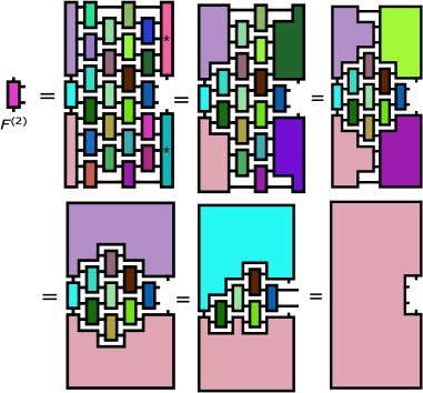
To complete the single tensor optimization, we need to perform the actual computation of the tensor , i.e. we need a strategy for contracting the tensor network of Fig. 4C.
The order in which the contractions are performed has a large impact on the final computation cost. In the case of a deep circuit with few qubits, a “horizontal” contraction order (e.g. from left to right) will save computation cost. The horizontal contraction order corresponds to what is done in Schrödinger-like simulations. Its cost is prohibitive for a large number of qubits due to its exponential memory footprint . Here, however, we consider only a shallow circuit of only a few layers at a time, so it is advantageous to perform the contraction in “vertical” order (e.g. from top to bottom) since the exponential cost is with respect to instead of . This contraction algorithm is a direct adaptation of the well-known algorithm for calculating the scalar product between two MPS’s Schollwöck (2011).
An example of contraction path for is shown in Fig. 5. We first perform trivial contractions such as contracting one-qubit gates with nearby two-qubit gates. Then, we contract the first top line of tensors and move down until we have reached the (missing) tensor that is being optimized. We repeat the same procedure from the bottom of the network upwards up to the missing . Last, we merge the bottom part with the top part. Through out the tensor network contraction, the largest tensors have physical indices (corresponding to the horizontal edges) and virtual indices (corresponding to the vertical edges). Each physical index represents qubits, and thus has dimension ; each virtual index has dimension . The typical maximum memory footprint for large thus scales as . This is much smaller than the scaling that one would be facing with a naive horizontal contraction path.
Note that all the tensor network techniques discussed in Section II (heuristics for contraction paths, slicing…) could be used here to optimize and/or parallelize the calculation of .
IV.3 Open versus closed simulation mode
The algorithm can be used in two modes, open or closed, as discussed in section II. The open, “Schrödinger-like” mode provides the full quantum state after the layers of the circuit. One simply adds layers at a time using the compression step until one has added all the layers.
In the closed simulation mode, we seek to calculate an amplitude
| (22) |
for a fixed output bitstring . A closed simulation calculation corresponds to the overlap of two MPS’s, namely and , which can be calculated with two separate open calculations whose circuit depths are halved compared to the open simulation mode. Since calculations at small depths give much better fidelities with our technique (there is less entanglement at small depth) the overall error rate is much lower.
In practice, we first partition the circuit into three subcircuits with respectively , and layers,
| (23) |
Then, we perform an open simulation with the first layers of the circuit (the forward part),
| (24) |
Then, we perform a second open simulation starting from the product state with the last layers of the circuit (the backward part):
| (25) |
Last, we add the remaining layers and compute the remaining scalar product without approximation, using a contraction strategy analogous to the one used for the calculation of the :
| (26) |
The last calculation is performed exactly at the same cost as a compression step for . It may be advantageous to use and/or the corresponding bond dimensions if one wishes to calculate many different amplitudes . Indeed, the forward calculation needs to be done only once, while the backward and final calculations must be repeated for each bitstring . On the other hand, if one seeks the best possible fidelity, one should increase as much as possible in order to reduce the depth of the approximate parts of the calculation.
V Details on the numerical experiments
V.1 Three quantum circuits
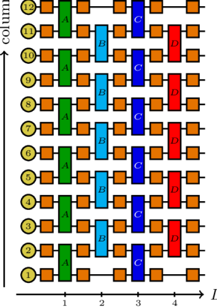
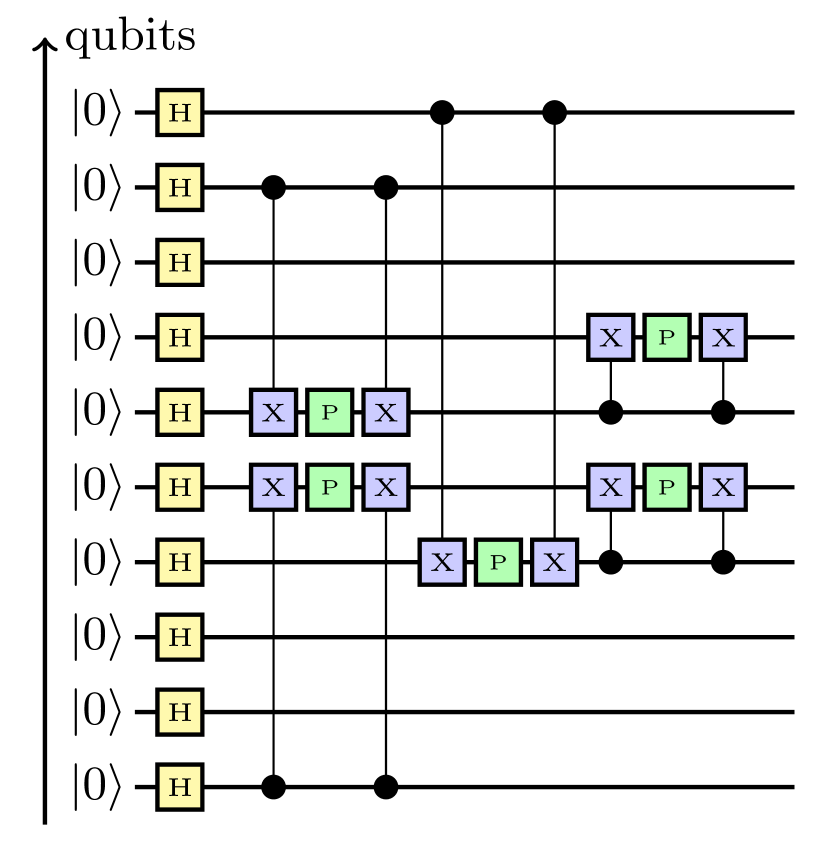
In this article, we performed numerical experiments with three different quantum circuits, labeled sequence I, II and III as discussed in section III. A schematic of the three sequences is shown in Fig. 6(a), Fig. 6(b) and Fig. 6(c) respectively.
Sequence I corresponds to the circuit of the quantum supremacy experiment, as shown on Fig. 6(a). It is designed to create a state as entangled as possible in as few steps as possible given the available nearest-neighbor connectivity. Each of the layers (where denotes the depth of the circuit, in the experiment) alternates between a one-qubit gate applied on all qubits (orange squares, drawn randomly from the , and gates) and a two-qubit gate applied on a set of pairs of qubits, with four possible sets denoted by the letters A, B, C and D as shown in Fig. 1 (A: green, B: light blue, C: dark blue and D: red rectangles). The two-qubit gate is the gate defined in Ref. Arute et al. (2019). In the actual experiment, the values of and have been optimized for each pair of qubits to reach the best fidelity. Here we choose a constant value , that is close to the average experimental one, and deep in the difficult regime where the fsim gate has four different singular values. We also use the same sequence ABCD-CDAB-ABCD-… as Arute et al. (2019) in the supremacy regime.
The alternative sequence II is a variation on the quantum supremacy sequence where we have changed the order of the gates applied. Sequence II is rotated by 90 degrees compared to sequence I and reads CDBA-BACD-CDBA-… This alternative sequence is just as useless but slightly “less random” than the supremacy sequence, since we have not designed it to be optimally random. This slight modification of the ordering has a strong impact of the fidelity found in the simulations.
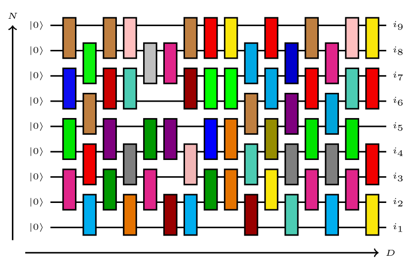
Finally, we benchmarked our DMRG algorithm on a useful task, sequence III. Sequence III is actually not a specific sequence of gates but a protocol for generating circuits implementing the Quantum Approximate Optimization Algorithm (QAOA)Edward et al. (2014) for solving MaxCut problems of combinatorial optimization. We generated many such problems for the “Sycamore” chip and selected instances where the associated QAOA circuit had a two-qubit gate count similar to the gate count of sequence I and II. Fig. 6(c) shows an example of such a circuit for a small number of qubits ().
More specifically, we solve the MaxCut problem on Erdos-Renyi graphs , a particular class of random graphs with vertices and a probability for creating an edge between two vertices. The QAOA ansatz circuit Edward et al. (2014) is of the form , with and , with the set of edges of the graph. Here, we are not interested in the result of the optimization itself. Hence, we set the variational parameters and to random values. For the same reason, we set the number of QAOA layers to 1. The edge density in the Erdos-Renyi graphs is adjusted so that the final two-qubit gate count is close to 430. We consider two different cases: without and with compilation. In the absence of compilation, the QAOA circuits do not necessarily comply with the grid connectivity of Sycamore (Fig. 1). To get a number of gates of about 430, we pick . In the second case, we compile the QAOA circuit to comply with the connectivity of Sycamore. The compilation uses SWAP insertion methods Hirata et al. (2009) to create a circuit that uses only the nearest neighbor two qubit gates available in Sycamore. As this procedure increases the depth of the circuit, we lower the edge probability down to to keep the final two-qubit gate count to 430.
V.2 Estimating the fidelity of a DMRG simulation
A very interesting feature of the DMRG algorithm is that the fidelity of the calculation can be easily estimated, even though we do not necessarily have access to the actual perfect state . Inside a simulation, we estimate the fidelity with
| (27) |
where the partial fidelities are the final fidelities of compression step
| (28) |
at the end of the different optimization sweeps. is simply given by the norm of the last tensor calculated during the compression step. It follows that our estimate of the error rate reads
| (29) |
It was shown in Ref. Zhou et al. (2020) through a combination of analytical and numerical arguments, that to very good approximation, one has
| (30) |
and the arguments and numerics given there remain valid for this article. However, since we have used a different compression algorithm here, we have performed an additional extensive numerical study of the validity of the multiplicative law [Eq. (30)] for up to a maximum of qubits for which we can obtain the exact state , hence the exact fidelity . The multiplicative law Eq. (27) has a very important role, as it allows us to perform estimations of the fidelities in regimes where the exact calculation is out of reach and only can be obtained. We have found that Eq. (30) indeed holds in all regimes of interest.
Fig. 10 shows the comparison between the exact fidelity (blue line) and our estimate (dashed blue line) for a large choice of values of and up to qubits (beyond that, we do not have access to the exact state ). We find a perfect match between the two curves in the relevant regime. For very large depth saturates at an exponentially small value while continues to decrease exponentially. The exponentially small asymptotic value corresponds to the overlap between two independent Porter-Thomas chaotic vectors, see the derivation around Eq. (38). It is essentially the lowest fidelity that can be reached in a random circuit.
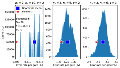
Interestingly, Eq. (27) provides an estimate of the error even in the closed mode where we calculate a single amplitude . To check this assertion, we have computed the histogram of the error rates per gate in the closed mode for small systems where we could calculate all the amplitudes exactly. Typical results are shown in Figure 8(b) for three different configurations. We find that our estimated fidelity closely matches the actual value with a precision of a few percent (typically less than ) for all the points in the histogram. Note that in all regimes we have so that underestimates the actual fidelity.
V.3 Different groupings of the qubits
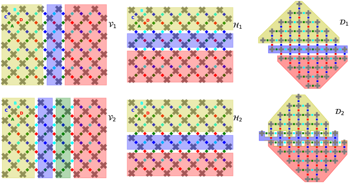
Our DMRG algorithm gives us the freedom to define how we group the different qubits that correspond to each tensor , . The different groupings that we have used are shown in Fig. 7, where each color corresponds to one tensor .
Different groupings may have some advantage depending on the actual circuit ran. The vertical groupings and group the qubits by columns. For instance contains three tensors with respectively (), () and () columns (qubits). Layers B and D are “trivial” for grouping , i.e. they are internal to one tensor hence have a perfect fidelity for any value of the bond dimension . Likewise, layers A and C are trivial for grouping . For the larger systems of Fig. 2(c) with more than qubits, we have used an extension of and by adding additional tensors of two columns to obtain qubits with tensors having respectively and qubits. We find that the vertical groupings are optimum for sequence II.
Another possibility is to group the qubits horizontally in rows as in (for which A and D are trivial), or (for which B and C are trivial). Last, we may group the qubits diagonally as in and . In some calculations, we may try and alternate between two groupings e.g. and to optimize the number of trivial gates.
V.4 Benchmark of the algorithm
Let us now see how the algorithm performs in practice. All the simulations are carried out on a Sycamore-like architecture with columns where each column has (odd) or (even) qubits, as shown in Fig. 1. The real Sycamore chip corresponds to qubits arranged in columns with qubits in the first column. We also performed simulations on smaller systems where we could obtain the exact state (up to qubits) using Atos QLM’s Schrödinger-style “qat-linalg” simulator.
V.4.1 Convergence of the DMRG compression step
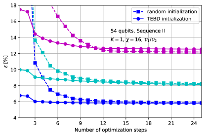
Fig. 8(a) shows the convergence of the optimized MPS during the DMRG sweeps. We plot the error per gate as a function of the number of optimization steps. Here is the number of two-qubit gates in the newly added layers and is the fidelity obtained upon optimizing tensor in sweep . Since the corresponding MPS contains tensors, optimization steps correspond to one full sweep. Since each step provides a full optimization over one tensor, the error rates decreases monotonically, as expected.
Fig. 8(a) shows two types of initialization of the MPS that is being optimized: either an arbitrary random MPS (squares and dashed lines) or an already partially optimized MPS obtained from the TEBD algorithm of Ref. Zhou et al. (2020) (disks and solid lines). By construction, the DMRG error can only be lower than the TEBD error. Unsurprisingly, we find that the convergence is much faster when starting from TEBD (typically sweeps) than when starting from a random guess (typically sweeps). However, the final error found shows weak dependence on the initial starting point (in Fig. 8(a) we show one case (pink curves) where there is a visible difference between the TEBD initialization and the random ones, but it is seldom observed). We have also repeated the simulation with different random initializations and the error always converges to the same value. Since we optimize only one tensor at a time, we cannot dismiss the possibility to be trapped in a local minimum but these observations indicate that the DMRG algorithm gets at least very close to the global optimum MPS. Note that this is the global optimum MPS for a given compression step. In section VI, we shall discuss how the algorithm manages to track the global optimum for the full circuit after several compression steps.
V.4.2 Role of the number of layers per step and number of sweeps
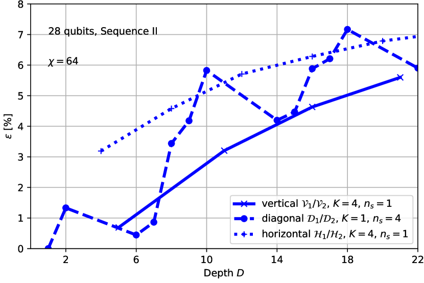
In most of the numerical experiments shown in this article, we have used the vertical ordering with , or the diagonal ordering with , . In the grouping, “even” layers of type B and D (see Fig. 7) can be absorbed trivially in the MPS without increasing the bond dimension. It follows that the fidelity for and is actually the same. We have performed a few simulations in the grouping with . They present a small, typically gain with respect to in return for -fold increase in computing time. Note that this gain reflects our ability to find the MPS closest to , not the ability of the MPS to capture the exact state. Indeed, the and calculations share the same bond dimension, and hence the same maximum level of possible entanglement.
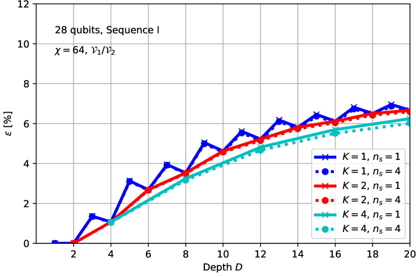
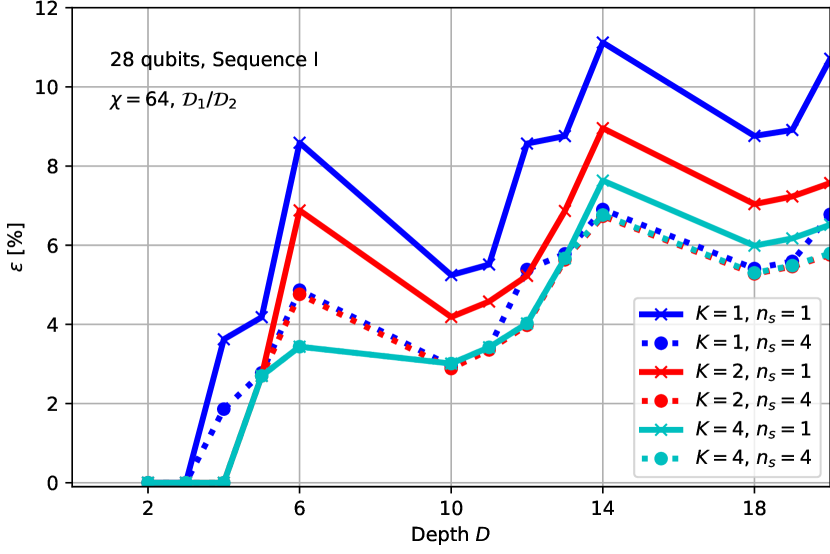
Fig. 8(c) shows the error rate as a function of the depth for different values of the number of layers added inside the compression step, for the vertical grouping . The error rate for depth is zero as our MPS has a bond dimension large enough to accomodate the corresponding entanglement exactly. As one increases further, one starts to feel the approximation and the error rate increases. As mentioned above, the error rates for and are identical with additional oscillations for the intermediate points for . This increase in the error rate for intermediate points for corresponds to the fact that these depths do not benefit from an upcoming trivial layer, hence the average error rate is higher. For , we observe a small gain at large depths, but since the corresponding computational time increases significantly, we have not used in practice. Similar calculations for the diagonal grouping are shown in Fig. 8(d). The error rate shows oscillations due to the fact that, in this configuration, the gate is very costly. Overall, we find that for a large enough number of sweeps , the dependence of the error rate is small. This is already a strong indication that the algorithm provides a MPS not far from optimum, even though we are carrying out multiple compression steps. Increasing the number of layers provides a small gain of in the error rate at . However the computational cost increases exponentially with . Calculations with 54 qubits and are beyond the scope of the present article for the diagonal grouping.
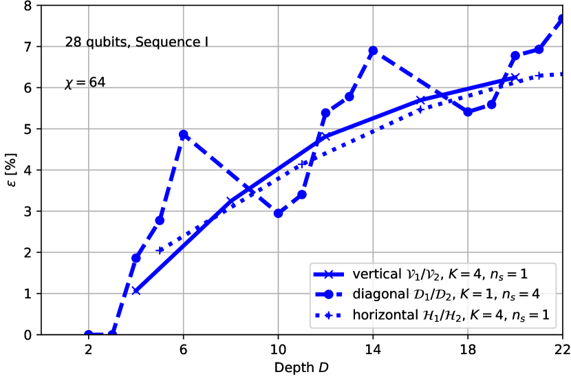
V.4.3 Role of the qubit grouping
Figs. 8(e) and 8(f) show the error rate versus depth for three different groupings, vertical, diagonal and horizontal. We observe important variations of the error rate with the grouping as well as with the circuit (sequence I versus sequence II). Note that for this small system of qubits (, ), sequence II is only marginally easier than sequence I because the system is almost like a square (as opposed to a rectangle for the Sycamore case , ). This difference between different groupings is in itself not surprising: different circuits tend to entangle some qubits more than others. Since the choice of the grouping amounts to choosing the position of “entanglement bottleneck”, there must be an optimum grouping for each circuit.
VI Does DMRG provide the optimal MPS?
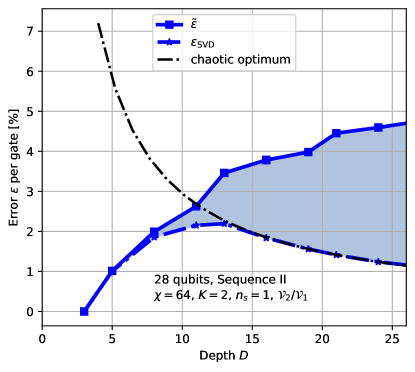
In this section, we discuss whether the MPS obtained by the DMRG algorithm corresponds to the best possible MPS. Indeed, two possible causes may prevent the final MPS obtained to be optimal: the fact that the optimization is broken into different compression steps, and the fact that within a compression step the optimization is performed tensor by tensor, not globally. We analyze this problem in the context of the random circuit of sequence II.
To assess this point, Fig. 9 shows three different errors versus depth curves:
-
•
The blue squares (continuous line) show the error obtained within the DMRG algorithm
-
•
The blue stars (dashed line) show the error corresponding to best possible approximation of the exact state with a MPS, as explained below. This reference curve can only be obtained for a small number of qubits and is not available in general.
-
•
The black dot-dashed line shows the error , the best possible approximation of a purely chaotic state with a MPS, as given by
(31) (see the analytical derivation below, appendix B). We refer to Eq. (31) as the “chaotic optimum error”. The fact that the chaotic optimum error decreases with stems from the simple fact that the best fidelity that one may obtain when approximating a chaotic state with a MPS is a finite number so that the error per gate must decrease.
VI.1 Best possible MPS calculation
To obtain the blue stars (dashed line) “best possible MPS” curve of Fig. 9, we performed an exact “Schrödinger-like” simulation of the small -qubit system and obtained the exact state .
In a second step, we split the qubits into two groups A and B of equal size, so that reads
| (32) |
where the states ( ) form an orthonormal basis of A (B). We perform a singular value decomposition of the matrix, , from which we get the Schmidt decomposition of :
| (33) |
with (and a similar expression for ). Sorting the singular values in decreasing order, we can obtain the best approximate MPS by truncating the above expression and keeping the largest singular values.
VI.2 Analytical calculation of the chaotic optimum Eq. (31)
The computation of the chaotic optimum Eq. (31) follows the same procedure as for the “best possible MPS” discussed above with a small modification: instead of starting with the exact state , we start with a fully chaotic state distributed according to the Porter-Thomas distribution, i.e.
| (34) |
where and the Porter-Thomas vector corresponds to one column of a unitary matrix distributed according to the Haar (uniform) measure of .
The derivation of the “chaotic optimum” error formula follows from the properties of the singular values of random Gaussian matrices. It is performed in Appendix B.
VI.3 Numerical results
We find in Fig. 9 that the best possible error first increases as the system gets more and more entangled; reaches a maximum at ; and then starts to decrease following closely the chaotic optimum. The maximum error at hence corresponds to the depth beyond which the state of the system is chaotic.
In contrast, in our DMRG simulations the error can, by construction, only increase. It eventually saturates to a finite value when the MPS becomes made of random tensors (see an in-depth discussion of this last point in Zhou et al. (2020)). Hence, it must deviate from the best possible approximation at some point. Fig. 9 shows that this deviation appears around when the system becomes chaotic. At small depths, the DMRG results are indeed very close to the best possible approximation. From Fig. 9 data, we conjecture that the intersection between the DMRG error and the chaotic optimum can be used to estimate when the quantum state becomes chaotic. Before one reaches the chaotic regime, the DMRG algorithm is close to optimum. Conversely, Fig. 9 can be seen as a strong indication that for non-chaotic states, DMRG will perform significantly better than for chaotic ones.
VII Relation between fidelity and cross-entropy benchmarking
The relation between the actual fidelity and the cross-entropy benchmarking is far from trivial. Ref. Arute et al. (2019) has argued that in their experiment and in the large-depth chaotic regime both quantities are equivalent , see also Zhou et al. (2020) for a discussion.
Here we show that in our numerics we have a very different relation
| (35) |
which implies that (since ). We give two kinds of evidence for Eq. (35):
-
•
A large body of numerical caculations for systems up to qubits where we can simulate the exact state , hence calculate both the left and right-hand side of Eq. (35)
-
•
An analytical calculation in the very large limit. In this limit, and converge to two independent random chaotic states and one can calculate the two fidelities exactly and show that Eq. (35) holds. It follows that the type of errors present in an experiment plays an important role to know which relation holds: assuming that one only makes precision errors experimentally (such as over rotations during a gate), one would retain a pure state at large depth and Eq. (35) would hold.
These two bodies of evidence are presented in the rest of this section.
VII.1 Numerical evidence for
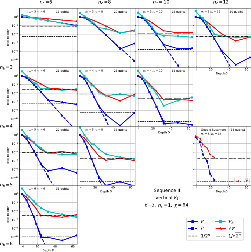
Fig. 10 shows (blue) and (green) for several values of and for which , so that the exact state could be obtained using the large random access memory (RAM) of the Atos Quantum Learning Machine. Also shown is (red), which is close to the green curve as well as the two exact asymptotic values for and for . As one gets closer to the Sycamore chip regime (, ), for which no exact statement can be made, we find that the relation becomes increasingly valid.
VII.2 Fidelity and cross-entropy benchmarking in the chaotic limit
In this subsection, we calculate and analytically in the limit. In this limit, the two states and become essentially independent and distributed according to a Porter-Thomas distribution. Let us denote and and two matrices distributed according to the Haar (uniform) measure of the group. With these notations, the two states are, for very large depths, the first column of the matrices and : and . We further denote the average over these ensembles. We will make use of two integrals that can be found in Brouwer and Beenakker (1996): for any matrices and , one has
| (36) |
and
Using the first of these two integrals, we obtain
| (38) |
and
| (39) |
Since vanishes in average, we need to calculate its variance to estimate its typical value. We get
| (40) |
After some straightforward algebra, we get
| (41) |
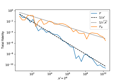
It follows that at very large depths, . Fig. 11 shows a numerical calculation of and for two independent Porter-Thomas vectors together with the analytical expressions derived above.
VIII Conclusions
We have presented an algorithm to efficiently simulate quantum circuits with finite fidelity. This algorithm extends Ref. Zhou et al. (2020), where some of us adapted the time-evolving bond-decimation (TEBD) technique from many-body physics to the context of quantum circuits. Here we have introduced a generalization of the density-matrix renormalization group (DMRG) algorithm to quantum circuits. This new algorithm also has a simulation cost that scales polynomially with the number of qubits and the depth of the circuit . In addition, it is more general and more efficient than the previous TEBD-like algorithm. From the simulation point of view, we emphasize that the main building block of our DMRG algorithm, the “compression step”, is completely general and could be used in other contexts. In particular, it may be combined with other tensor network techniques such as slicing or contraction heuristics as in Refs. Pan and Zhang (2021); Gray and Kourtis (2021). These generalisations have not been attempted yet.
We have benchmarked our algorithm on the supremacy sequence designed by Google and found that we can produce amplitudes (hence bitstrings) of quality as good as in the quantum supremacy experiment Arute et al. (2019). More importantly, for QAOA sequences, representative of useful applications of quantum computers, we obtain much better fidelities than the supremacy threshold set by Google. Our results provide strong evidence that quantum advantage (the ability for a quantum computer to perform a useful task better than a classical computer) might be much harder than reaching quantum supremacy (the ability for a quantum computer to perform a given, not necessarily useful, task that no classical computer can perform), despite what the words seem to indicate. In particular, since our algorithm scales polynomially with the number of qubits, an improvement in the experimental fidelity is needed in order for the experiments to reach better results than the DMRG algorithm for useful tasks.
Our work emphasizes the need for benchmarks of quantum computers that test the actual usefulness of quantum processors, rather than their ability to perform a relatively contrived task, in order to incentivize hardware and software efforts towards concrete applications. Such benchmarks should strive to be application-centric, hardware-agnostic and scalable. Some of us recently proposed a protocol fulfilling these criteria Martiel et al. (2021).
Acknowledgments
We thank Giuseppe Carleo, Lei Wang, and Pan Zhang for helpful feedback about prior work in simulating quantum circuits and for pointing out several errors in the literature discussion. XW acknowledges funding from the French ANR QCONTROL as wel as the Plan France 2030 ANR-22-PETQ-0007. TL, XW and TA acknowledge funding from ANR QPEG. XW acknowledges funding from the European Union’s Horizon 2020 research and innovation programme under grant agreement No. 862683 (UltraFastNano). EMS acknowledges helpful discussions with Soonwon Choi on the topic of cross-entropy benchmarking and fidelity. The Flatiron Institute is a division of the Simons Foundation. The computations were performed on the Atos Quantum Learning Machine.
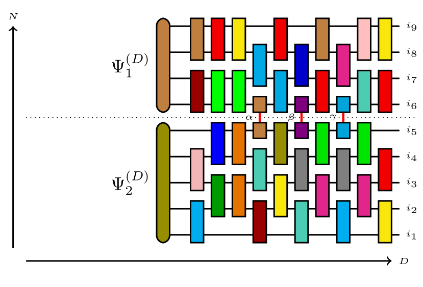
Appendix A A short introduction to tensor networks for simulating quantum circuits
In this appendix, we briefly review the main aspects of tensor networks in the context of quantum circuit simulation.
A.1 Basic definitions and actions: contracting and splitting
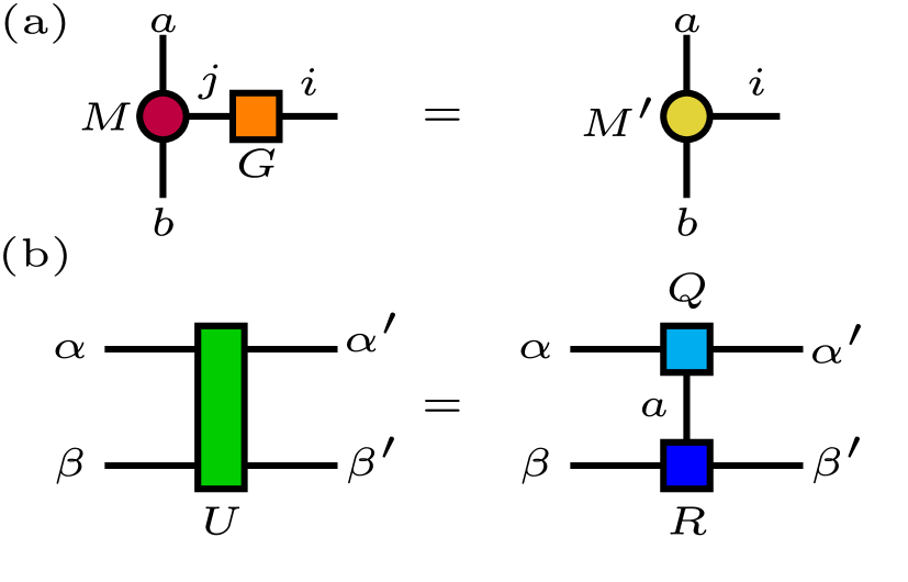
A tensor is simply an array of complex numbers that generalizes the concepts of vectors (1D array) and matrices (2D arrays) to an arbitray number of indices. A tensor with one index (that takes a finite number of values) is simply a vector; a tensor with two indices is a matrix; a tensor () is a 3D (4D) array of numbers. A tensor is represented graphically by a box (here a rectangle or a circle) with as many legs (outgoing lines) as there are indices, see examples in Fig. S1.
There are two basic operations that one can do with tensors: contracting and splitting. Contractions of two tensors is the generalization of matrix-matrix multiplication. An example is shown in Fig. S1b for the contraction of with . The resulting tensor is simply given by
| (42) |
i.e. one performs a summation over the index that links the two tensors.
The second operation, splitting of e.g. a tensor , is illustrated in Fig. S1c. It consists of three steps. First, one constructs two meta-indices and that group several indices together. For instance, one may choose and where and are the number of different values that the indices and take, respectively. This allows us to define a one-to-one mapping between the tensor and a matrix defined as
| (43) |
Second, we may use any result known from linear algebra on the matrix , for instance a QR decomposition, a SVD decomposition or any other decomposition. Let us suppose we use a QR decomposition and write . Third, we use the mapping Eq. (43) backward to go back to the original indices and obtain
| (44) |
i.e. we have split the tensor in terms of the contraction of two tensors and .
A.2 Tensor networks for quantum circuits
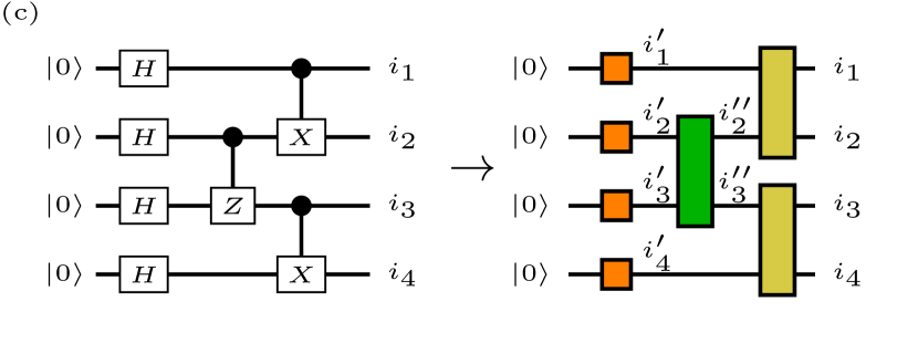
There is a natural correspondence between the usual representation for quantum circuits and tensor networks. The left-hand side of Fig. S1c shows a small quantum circuit for four qubits that uses the standard Hadamard gate , the control-NOT gate and the control-Z gate . The system wave-function is a tensor whose explicit form is given by
| (45) | |||||
i.e. it corresponds to the contraction of the tensor network shown on the right-hand side of Fig. S1c. The problem of computing the wave-function is reduced to the problem of performing the summation over the internal indices, i.e. the contraction of the tensor network Markov and Shi (2008). Finding the best order to perform the contraction is in general a difficult (NP hard) problem for which there nevertheless exists good heuristics.
A.3 Schrödinger versus Schrödinger-Feynman-like simulations
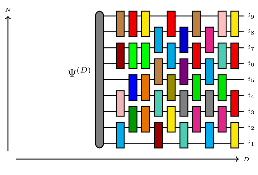
There are several possible different strategies to contract the tensor network associated with a quantum circuit. Fig. S2 shows two examples for the Schrödinger and the Schrödinger-Feynman approaches discussed in section II. In the Schrödinger approach, the contraction of the network is performed from left to right, as shown in Fig. 2(b). In the Schrödinger-Feynman approach, shown in Fig. 2(c), one divides the qubits into two groups and splits the two-qubit gates that connect the two groups. For a given value of the indices cut by the dotted line, one may propagate the two sub states and independently, see (9) and (10) from the main text. Thus instead of one complex simulation of the whole circuit, we perform easier simulations, where is the number of values taken by the extra bond indices.
Appendix B Derivation of the chaotic optimum error (Eq. (31))
In this appendix, we prove that for a chaotic state distributed according to the Porter-Thomas distribution, the best possible fidelity that one may obtain by approximating it with a MPS is
| (46) |
To establish this result, the wavefunction is considered as a matrix where index labels half of the qubits and labels the other half. Performing a singular value decomposition of the matrix to obtain its singular values , the fidelity for a bond dimension is given by the largest singular values
| (47) |
The proof contains two parts:
-
•
establish that the matrix is, in the large limit, a complex Gaussian random matrix;
-
•
use known results from random matrix theory to obtain the distribution of singular values from which one can obtain Eq. (46) after a little algebra.
We perform these tasks below.
B.1 Construction of a Porter-Thomas state from random Gaussian variables
We want to establish that a Porter-Thomas state can be constructed from random Gaussian variables. We recall that the sum of the squares of random normal variables follows a (generalized) distribution with mean and variance
| (48) | ||||
| (49) |
Its probability density function is
| (50) |
Let us construct a wavefunction with complex amplitudes
| (51) |
and choose the real and imaginary components to be normally distributed:
| (52) | ||||
| (53) |
Let us first consider the probability
| (54) |
This random variable is a sum of normal variables. Applying formula (50) with and , we find
| (55) |
i.e the Porter-Thomas distribution, as expected.
Let us now check that is normalized in the large limit. Let us consider its norm
| (56) |
This random variable is also a sum of normal variables. We can apply formulae (48-49) with and , we find
| (57) | ||||
| (58) |
We have constructed a wavefunction whose norm is 1 on average, with a deviation to the average that vanishes exponentially fast as the number of qubits increases.
As a result, the matrix is a random complex Gaussian matrix, up to exponentially small corrections. Let us note that the Gaussian probability distribution that we have used,
| (59) |
obviously respects the Haar invariance
| (60) |
for any unitary rotation with and for all . It is only the constraint which is enforced only in average with an exponentially small variance.
B.2 Scaling law for the singular values of a Porter-Thomas state
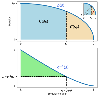

In this subsection, our goal is to understand how the Schmidt coefficients of the Porter-Thomas state constructed in the previous subsection decrease as a function of the index : a fast decrease will be synonymous of a high MPS quality.
For this purpose, we make use of known results from random matrix theory. More specifically, we use the fact that, in the large- limit, the average density of the singular values of a random complex Gaussian matrix (with matrix elements , ), as discussed in the previous subsection) follows a quadrant law (see e.g Shen (2001)):
| (61) |
In the large- limit, the number of singular values above a given threshold is given by
| (62) |
Inverting the above function provides the sought-after scaling of the singular values, . Introducing the rescaled singular value , we get
| (63) |
with
| (64) |
It follows that follows a scaling law
| (65) |
where the function is the inverse of , as illustrated in the lower panel of Fig. S3. The function corresponds to the area of a portion of a (distorted) circle and can be computed using a simple geometrical argument. Introducing the angle (see inset of Fig. S3), one obtains
| (66) |
with . We therefore obtain
| (67) |
In particular, one has and .
This scaling law can be used to derive the behavior of the error rate in the chaotic limit, Eq. (31). Truncating the original wave vector (Eq. (33)) to its first eigenvalues () yields the fidelity . Thus, using Eq. (65),
| (68) |
and in the limit we obtain the advertised chaotic limit:
| (69) |
and the associated value for the error rate . Interestingly, plateaus at for large .
We note that if all the singular values were equal (), then we would have and hence (following Eq. (68)), namely one fourth of the leading term of Eq. (69). In other terms, the fidelity in the chaotic limit is only times larger than in the worst possible situation where all the singular values are of equal importance.
We check in Fig. S4 that this scaling law of the singular values can indeed be observed. We perform a SVD decomposition of the random vector obtained by the procedure described in the previous subsection, and plot the corresponding function properly rescaled. The result is almost indistinguishable from the analytical function calculated above.
Appendix C Metropolis sampling for closed simulations
To produce the same output as a quantum computer within the framework of closed simulations, one must be able to sample from the distribution . This means not only computing amplitudes for a given bitstring but producing bitstrings distributed following . A simple general algorithm for this task has been proposed in Bravyi et al. (2021) (see also the discussion in section II). The algorithm of Bravyi et al. (2021) requires the calculations of amplitudes per bitstring. In the case of random circuits such as sequence I and II, this is far from optimum. A possible strategy is to use the Metropolis algorithm to construct a Markov chain of bitstrings : one picks at random and accepts the proposed value with the probability (acceptance ratio). If the proposed move is refused then . In the random circuit of quantum supremacy, one quickly reaches a Porter-Thomas distribution, i.e. the amplitudes are themselves distributed according to an exponential law . It follows that the average acceptance ratio is fairly large:
| (70) |
i.e. in average bitstrings must be calculated in order to get a new accepted bitstring.
If one wanted to pretend that the bitstrings came from an actual quantum computer, one would want to be almost certain that a given bitstring could not appear twice consecutively. In that case, one would want to keep only one bitstring every Metropolis update, hence lowering the probability of repetition to about . For , this would give a very low repetition probability of . However, this precaution can probably be skipped as the cross-entropy benchmarking fidelity can easily be spoofed: simply ignoring the repeated values would create a bias in the distribution that would probably be very hard if not impossible to detect. Hence one or two amplitudes per bitstring should be enough in practice.
References
- Arute et al. (2019) Frank Arute, Kunal Arya, Ryan Babbush, Dave Bacon, Joseph C. Bardin, Rami Barends, Rupak Biswas, Sergio Boixo, Fernando G. S. L. Brandao, David A. Buell, and et al., “Quantum supremacy using a programmable superconducting processor,” Nature 574, 505–510 (2019).
- Bauer et al. (2020) Bela Bauer, Sergey Bravyi, Mario Motta, and Garnet Kin-Lic Chan, “Quantum Algorithms for Quantum Chemistry and Quantum Materials Science,” Chemical Reviews 120, 12685–12717 (2020), arXiv:2001.03685 .
- Reiher et al. (2017) Markus Reiher, Nathan Wiebe, Krysta M Svore, Dave Wecker, and Matthias Troyer, “Elucidating reaction mechanisms on quantum computers,” Proceedings of the National Academy of Sciences 114, 7555–7560 (2017), arXiv:1605.03590 .
- Gray and Kourtis (2021) Johnnie Gray and Stefanos Kourtis, “Hyper-optimized tensor network contraction,” Quantum 5, 410 (2021).
- Pan and Zhang (2021) Feng Pan and Pan Zhang, “Simulating the sycamore quantum supremacy circuits,” (2021), arXiv:2103.03074 [quant-ph] .
- Pan et al. (2022) Feng Pan, Keyang Chen, and Pan Zhang, “Solving the sampling problem of the sycamore quantum circuits,” Phys. Rev. Lett. 129, 090502 (2022).
- Zhou et al. (2020) Yiqing Zhou, E. Miles Stoudenmire, and Xavier Waintal, “What limits the simulation of quantum computers?” Phys. Rev. X 10, 041038 (2020).
- Daley et al. (2004) A J Daley, C Kollath, U Schollwöck, and G Vidal, “Time-dependent density-matrix renormalization-group using adaptive effective hilbert spaces,” Journal of Statistical Mechanics: Theory and Experiment 2004, P04005 (2004).
- Vidal (2004) Guifré Vidal, “Efficient simulation of one-dimensional quantum many-body systems,” Phys. Rev. Lett. 93, 040502 (2004).
- White and Feiguin (2004) Steven R. White and Adrian E. Feiguin, “Real-time evolution using the density matrix renormalization group,” Phys. Rev. Lett. 93, 076401 (2004).
- White (1993) Steven R. White, “Density-matrix algorithms for quantum renormalization groups,” Phys. Rev. B 48, 10345–10356 (1993).
- Schollwöck (2011) U. Schollwöck, “The density-matrix renormalization group in the age of matrix product states,” Annals of Physics 326, 96–192 (2011).
- Edward et al. (2014) Farhi Edward, Goldstone Jeffrey, and Gutmann Sam, “A Quantum Approximate Optimization Algorithm,” (2014), arXiv:1411.4028 .
- Wu et al. (2021) Yulin Wu, Wan-su Bao, Sirui Cao, Fusheng Chen, Ming-Cheng Chen, Xiawei Chen, Tung-Hsun Chung, Hui Deng, Yajie Du, Daojin Fan, Ming Gong, Cheng Guo, Chu Guo, Shaojun Guo, Lianchen Han, Linyin Hong, He-liang Huang, Yong-heng Huo, Liping Li, Na Li, Shaowei Li, Yuan Li, Futian Liang, Chun Lin, Jin Lin, Haoran Qian, Dan Qiao, Hao Rong, Hong Su, Lihua Sun, Liangyuan Wang, Shiyu Wang, Dachao Wu, Yu Xu, Kai Yan, Weifeng Yang, Yang Yang, Yangsen Ye, Jianghan Yin, Chong Ying, Jiale Yu, Chen Zha, Cha Zhang, Haibin Zhang, Kaili Zhang, Yiming Zhang, Han Zhao, Youwei Zhao, Liang Zhou, Qingling Zhu, Chao-yang Lu, Cheng-zhi Peng, Xiaobo Zhu, and Jian-wei Pan, “Strong Quantum Computational Advantage Using a Superconducting Quantum Processor,” Physical Review Letters 127, 180501 (2021), arXiv:2106.14734 .
- Zhong et al. (2020) Han-Sen Zhong, Hui Wang, Yu-Hao Deng, Ming-Cheng Chen, Li-Chao Peng, Yi-Han Luo, Jian Qin, Dian Wu, Xing Ding, Yi Hu, Peng Hu, Xiao-Yan Yang, Wei-Jun Zhang, Hao Li, Yuxuan Li, Xiao Jiang, Lin Gan, Guangwen Yang, Lixing You, Zhen Wang, Li Li, Nai-Le Liu, Chao-Yang Lu, and Jian-Wei Pan, “Quantum computational advantage using photons,” Science 370, 1460–1463 (2020), https://science.sciencemag.org/content/370/6523/1460.full.pdf .
- Popova and Rubtsov (2021) A. S. Popova and A. N. Rubtsov, “Cracking the quantum advantage threshold for gaussian boson sampling,” (2021).
- Villalonga et al. (2021) Benjamin Villalonga, Murphy Yuezhen Niu, Li Li, Hartmut Neven, John C. Platt, Vadim N. Smelyanskiy, and Sergio Boixo, “Efficient approximation of experimental gaussian boson sampling,” (2021).
- Oh et al. (2022) Changhun Oh, Youngrong Lim, Bill Fefferman, and Liang Jiang, “Classical simulation of boson sampling based on graph structure,” Phys. Rev. Lett. 128, 190501 (2022).
- (19) Yong, Liu, Xin, Liu, Fang, Li, Haohuan Fu, Yuling Yang, Jiawei Song, Pengpeng Zhao, Zhen Wang, Dajia Peng, Huarong Chen, Chu Guo, Heliang Huang, Wenzhao Wu, and Dexun Chen, “Closing the ”quantum supremacy” gap: Achieving real-time simulation of a random quantum circuit using a new sunway supercomputer,” 10.1145/3458817.3487399, 2110.14502v2 .
- Arute et al. (2020) Frank Arute, Kunal Arya, Ryan Babbush, Dave Bacon, Joseph C. Bardin, Rami Barends, Sergio Boixo, Michael Broughton, Bob B. Buckley, David A. Buell, Brian Burkett, Nicholas Bushnell, Yu Chen, Zijun Chen, Benjamin Chiaro, Roberto Collins, William Courtney, Sean Demura, Andrew Dunsworth, Edward Farhi, Austin Fowler, Brooks Foxen, Craig Gidney, Marissa Giustina, Rob Graff, Steve Habegger, Matthew P. Harrigan, Alan Ho, Sabrina Hong, Trent Huang, William J. Huggins, Lev Ioffe, Sergei V. Isakov, Evan Jeffrey, Zhang Jiang, Cody Jones, Dvir Kafri, Kostyantyn Kechedzhi, Julian Kelly, Seon Kim, Paul V. Klimov, Alexander Korotkov, Fedor Kostritsa, David Landhuis, Pavel Laptev, Mike Lindmark, Erik Lucero, Orion Martin, John M. Martinis, Jarrod R. McClean, Matt McEwen, Anthony Megrant, Xiao Mi, Masoud Mohseni, Wojciech Mruczkiewicz, Josh Mutus, Ofer Naaman, Matthew Neeley, Charles Neill, Hartmut Neven, Murphy Yuezhen Niu, Thomas E. O’Brien, Eric Ostby, Andre Petukhov, Harald Putterman, Chris Quintana, Pedram Roushan, Nicholas C. Rubin, Daniel Sank, Kevin J. Satzinger, Vadim Smelyanskiy, Doug Strain, Kevin J. Sung, Marco Szalay, Tyler Y. Takeshita, Amit Vainsencher, Theodore White, Nathan Wiebe, Z. Jamie Yao, Ping Yeh, and Adam Zalcman, “Hartree-Fock on a superconducting qubit quantum computer,” (2020), arXiv:2004.04174 .
- Pednault et al. (2019) Edwin Pednault, John A. Gunnels, Giacomo Nannicini, Lior Horesh, and Robert Wisnieff, “Leveraging secondary storage to simulate deep 54-qubit sycamore circuits,” (2019), arXiv:1910.09534 .
- Bravyi et al. (2021) Sergey Bravyi, David Gosset, and Yinchen Liu, “How to simulate quantum measurement without computing marginals,” (2021), 2112.08499v2 .
- Huang et al. (2020) Cupjin Huang, Fang Zhang, Michael Newman, Junjie Cai, Xun Gao, Zhengxiong Tian, Junyin Wu, Haihong Xu, Huanjun Yu, Bo Yuan, Mario Szegedy, Yaoyun Shi, and Jianxin Chen, “Classical simulation of quantum supremacy circuits,” (2020), 2005.06787v1 .
- Harrigan et al. (2021) Matthew P. Harrigan, Kevin J. Sung, Matthew Neeley, Kevin J. Satzinger, Frank Arute, Kunal Arya, Juan Atalaya, Joseph C. Bardin, Rami Barends, Sergio Boixo, Michael Broughton, Bob B. Buckley, David A. Buell, Brian Burkett, Nicholas Bushnell, Yu Chen, Zijun Chen, Ben Chiaro, Roberto Collins, William Courtney, Sean Demura, Andrew Dunsworth, Daniel Eppens, Austin Fowler, Brooks Foxen, Craig Gidney, Marissa Giustina, Rob Graff, Steve Habegger, Alan Ho, Sabrina Hong, Trent Huang, L. B. Ioffe, Sergei V. Isakov, Evan Jeffrey, Zhang Jiang, Cody Jones, Dvir Kafri, Kostyantyn Kechedzhi, Julian Kelly, Seon Kim, Paul V. Klimov, Alexander N. Korotkov, Fedor Kostritsa, David Landhuis, Pavel Laptev, Mike Lindmark, Martin Leib, Orion Martin, John M. Martinis, Jarrod R. McClean, Matt McEwen, Anthony Megrant, Xiao Mi, Masoud Mohseni, Wojciech Mruczkiewicz, Josh Mutus, Ofer Naaman, Charles Neill, Florian Neukart, Murphy Yuezhen Niu, Thomas E. O’Brien, Bryan O’Gorman, Eric Ostby, Andre Petukhov, Harald Putterman, Chris Quintana, Pedram Roushan, Nicholas C. Rubin, Daniel Sank, Andrea Skolik, Vadim Smelyanskiy, Doug Strain, Michael Streif, Marco Szalay, Amit Vainsencher, Theodore White, Z. Jamie Yao, Ping Yeh, Adam Zalcman, Leo Zhou, Hartmut Neven, Dave Bacon, Erik Lucero, Edward Farhi, and Ryan Babbush, “Quantum approximate optimization of non-planar graph problems on a planar superconducting processor,” Nature Physics 17, 332–336 (2021), arXiv:2004.04197 .
- Gao et al. (2021) Xun Gao, Marcin Kalinowski, Chi-Ning Chou, Mikhail D. Lukin, Boaz Barak, and Soonwon Choi, “Limitations of linear cross-entropy as a measure for quantum advantage,” (2021).
- Pang et al. (2020) Yuchen Pang, Tianyi Hao, Annika Dugad, Yiqing Zhou, and Edgar Solomonik, “Efficient 2d tensor network simulation of quantum systems,” in SC20: International Conference for High Performance Computing, Networking, Storage and Analysis (2020) pp. 1–14.
- Lin et al. (2021) Sheng-Hsuan Lin, Michael Zaletel, and Frank Pollmann, “Efficient simulation of dynamics in two-dimensional quantum spin systems with isometric tensor networks,” (2021), 2112.08394 .
- Proctor et al. (2022) Timothy Proctor, Kenneth Rudinger, Kevin Young, Erik Nielsen, and Robin Blume-Kohout, “Measuring the capabilities of quantum computers,” Nature Physics 18, 75–79 (2022), arXiv:2008.11294 .
- Dupont et al. (2022) Maxime Dupont, Nicolas Didier, Mark J. Hodson, Joel E. Moore, and Matthew J. Reagor, “Calibrating the classical hardness of the quantum approximate optimization algorithm,” (2022).
- Sreedhar et al. (2022) Rishi Sreedhar, Pontus Vikstål, Marika Svensson, Andreas Ask, Göran Johansson, and Laura García-Álvarez, “The quantum approximate optimization algorithm performance with low entanglement and high circuit depth,” (2022).
- Medvidović and Carleo (2021) Matija Medvidović and Giuseppe Carleo, “Classical variational simulation of the Quantum Approximate Optimization Algorithm,” npj Quantum Information 7, 101 (2021).
- Jónsson et al. (2018) Bjarni Jónsson, Bela Bauer, and Giuseppe Carleo, “Neural-network states for the classical simulation of quantum computing,” (2018), arXiv:1808.05232 [quant-ph] .
- White (1992) Steven R. White, “Density matrix formulation for quantum renormalization groups,” Phys. Rev. Lett. 69, 2863–2866 (1992).
- Saberi et al. (2009) Hamed Saberi, Andreas Weichselbaum, Lucas Lamata, David Pérez-García, Jan von Delft, and Enrique Solano, “Constrained optimization of sequentially generated entangled multiqubit states,” Phys. Rev. A 80, 022334 (2009).
- Stoudenmire and White (2010) E M Stoudenmire and Steven R White, “Minimally entangled typical thermal state algorithms,” New Journal of Physics 12, 055026 (2010).
- Hirata et al. (2009) Yuichi Hirata, Masaki Nakanishi, Shigeru Yamashita, and Yasuhiko Nakashima, “An Efficient Method to Convert Arbitrary Quantum Circuits to Ones on a Linear Nearest Neighbor Architecture,” in 2009 Third International Conference on Quantum, Nano and Micro Technologies (IEEE, 2009) pp. 26–33.
- Brouwer and Beenakker (1996) P. W. Brouwer and C. W. J. Beenakker, “Diagrammatic method of integration over the unitary group, with applications to quantum transport in mesoscopic systems,” Journal of Mathematical Physics 37, 4904–4934 (1996).
- Martiel et al. (2021) Simon Martiel, Thomas Ayral, and Cyril Allouche, “Benchmarking quantum co-processors in an application-centric, hardware-agnostic and scalable way,” 4 (2021), arXiv:2102.12973 .
- Markov and Shi (2008) Igor L. Markov and Yaoyun. Shi, “Simulating quantum computation by contracting tensor networks,” SIAM Journal on Computing 38, 963–981 (2008), https://doi.org/10.1137/050644756 .
- Shen (2001) Jianhong Shen, “On the singular values of Gaussian random matrices,” Linear Algebra and its Applications 326, 1–14 (2001).