Lower bounds for eigenfunction restrictions in lacunary regions

Abstract.

Let $(M,g)$ be a compact, smooth Riemannian manifold and $\{u_{h}\}$ be a sequence of $L^{2}$-normalized Laplace eigenfunctions that has a localized defect measure $\mu$ in the sense that $M\setminus{\operatorname{supp\,}}\!(\pi_{*}\mu)\neq\emptyset$ where $\pi:T^{*}M\to M$ is the canonical projection. Using Carleman estimates we prove that for any real-smooth closed hypersurface $H\subset(M\setminus{\operatorname{supp\,}}\!(\pi_{*}\mu))$ sufficiently close to ${\operatorname{supp\,}}\!(\pi_{*}\mu),$ and for all $\delta>0,$

$$\int_{H}|u_{h}|^{2}d\sigma_{{}_{\!H}}\geq C_{\delta}e^{-[\,d(H,{\operatorname{supp\,}}\!(\pi_{*}\mu))+\delta\,]/h}$$

as $h\to 0^{+}$. We also show that the result holds for eigenfunctions of Schrödinger operators and give applications to eigenfunctions on warped products and joint eigenfunctions of quantum completely integrable (QCI) systems.

1. Introduction

Let $(M,g)$ be a compact, $C^{\infty}$ Riemannian manifold, with or without boundary. Let $\Delta_{g}$ be the Laplace operator, and consider $L^{2}$-normalized Laplace eigenfunctions $u_{h}\in C^{\infty}(M)$,

$$(-h^{2}\Delta_{g}-1)u_{h}=0,\qquad\qquad\|u_{h}\|_{{}_{\!L^{2}}}=1.$$ (1)

In the case where $\partial M\neq\emptyset$, we ask that the boundary be smooth and we impose that the $u_{h}$ satisfy either Dirichlet or Neumann boundary conditions on $\partial\Omega$. That is, we ask that either $u_{h}=0$ on $\partial M$ or $\partial_{\nu}u_{h}=0$ on $\partial M$, where $\partial_{\nu}$ is the normal derivative along the boundary.

Let $H\subset M$ be a smooth hypersurface. Quantitative unique continuation for eigenfunction restrictions $u_{h}|_{H}$ is an important property with applications to the study of eigenfunction nodal sets and has received a lot of attention in the literature over the past decade, e.g., [DF88, TZ09, BR15, ET15, CT18, GRS13, Jun14, JZ16, TZ21]. Specifically, let $\{u_{h_{j}}\}_{j}$ be a sequence of eigenfunctions. Then, the question of whether there exist constants $C_{{}_{\!H}}>0$ and $h_{0}>0$ such that

$$\int_{H}|u_{h_{j}}|^{2}d\sigma_{{}_{\!H}}\geq e^{-C_{{}_{\!H}}/h_{j}}$$ (2)

for all $h_{j}\in(0,h_{0}]$ is, in general, an open question. Here, $d\sigma_{{}_{\!H}}$ denotes the measure on $H$ induced by the Riemannian metric.

In principle, the validity of (2) depends on both the particular eigenfunction sequence and the geometry of the hypersurface $H.$ In the terminology of [TZ09], hypersurfaces $H$ for which (2) is satisfied are said to be good for the eigenfunction sequence $\{u_{h_{j}}\}_{j=1}^{\infty}.$ It is a much more subtle problem than the analogue for submanifolds $U\subset M$ with $\dim U=\dim M$; indeed, in the latter case, the estimate $\|u_{h}\|_{{}_{\!L^{2}(U)}}\geq e^{-C_{U}/h}$ follows by a well-known argument with Carleman estimates [Zw]. For the hypersurface analogue in (2), there are comparatively few cases where (2) has been proved [BR15, ET15, CT18, GRS13, Jun14].

Our first result in Theorem 1 deals with the case where the $u_{h}$’s have a defect measure, $\mu$, that is well-localized in the sense that ${\operatorname{supp\,}}\!(\pi_{*}\mu)\neq M$, where $\pi:T^{*}M\to M$ is the natural projection. See [Zw, Chapter 5] for background on defect measures. Roughly speaking, under this condition, our main result, Theorem 1, shows that (2) is satisfied for a wide class of real-smooth separating hypersurfaces $H\subset M\backslash{\operatorname{supp\,}}\!(\pi_{*}\mu)$ that lie near ${\operatorname{supp\,}}(\pi_{*}\mu)$.

Before stating our first result, we introduce the notion of a lacunary region. Throughout the paper, we write $\mathcal{U}_{{}_{\!H}}(\tau)$ for a Fermi collar neighbourhood of a hypersurface $H\subset M$ of width $\tau>0$ (see (19)). In the following, we work with $h$-pseudodifferential operators in $\Psi_{h}^{0}(\mathcal{U}_{{}_{\!H}}(\tau))$ that are properly-supported in the Fermi tube $\mathcal{U}_{{}_{\!H}}(\tau)$ (see Subsection 3.1 for the definition). In addition, given cutoffs $\chi_{1},\chi_{{}_{\!\,2}}\in C^{\infty}_{0}(\mathcal{U}_{{}_{\!H}}(\tau)),$ the notation $\chi_{{}_{\!\,2}}\Subset\chi_{{}_{\!\,1}}$ means that $\chi_{{}_{\!\,1}}\equiv 1$ on ${\operatorname{supp\,}}\chi_{{}_{\!\,2}}$

Definition 1.1 ($H$-lacunary region).

Let $M$ be a $C^{\infty}$ manifold, $H\subset M$ a closed $C^{\infty}$-hypersurface, and $\tau>0$ such that $\mathcal{U}_{{}_{\!H}}(\tau)$ is a Fermi collar neighborhood of $H$. An $h$-pseudodifferential operator $Q(h)\in\Psi_{h}^{0}(\mathcal{U}_{{}_{\!H}}(\tau))$ that is properly-supported in the Fermi tube $\mathcal{U}_{{}_{\!H}}(\tau)$ is said to be a lacunary operator for the sequence $\{u_{h}\}$ if:

(i) $Q(h)$ is $h$-elliptic on $T^{*}\mathcal{U}_{{}_{\!H}}(\tau)$ (see Definition 3.1),

(ii) for every $\chi_{{}_{\!\,1}},\chi_{{}_{\!\,2}}\in C^{\infty}_{0}(\mathcal{U}_{{}_{\!H}}(\tau),[0,1])$ with $\chi_{{}_{\!\,2}}\Subset\chi_{{}_{\!\,1}},$ there exists a constant $C>0$, depending only on the sequence $\{u_{h}\}$, such that

$$\|\chi_{{}_{\!\,2}}Q(h)\chi_{{}_{\!\,1}}\,\,u_{h}\|_{{}_{\!L^{2}(\mathcal{U}_{{}_{\!H}}(\tau))}}=O(e^{-C/h}),\qquad h\to 0^{+}.$$ (3)

We say that there is an $H$-lacunary region for the sequence $\{u_{h}\}$ provided there exist $\tau>0$ and a lacunary operator $Q(h)\in\Psi_{h}^{0}(\mathcal{U}_{{}_{\!H}}(\tau))$ for $\{u_{h}\}$.

Remark 1.2.

Since one can always replace $Q(h)$ with $Q(h)^{*}Q(h)$ in (3) above, without loss of generality, we also assume that the principal symbol $q_{0}$ is real-valued. Also, we note that in the case where $Q(h)$ is $h$-differential, since it is then local, one can replace (3) with the condition that $\|\chi_{{}_{\!\,2}}Q(h)\,u_{h}\|_{L^{2}}\leq C_{0}\,e^{-C/h}\|u_{h}\|_{L^{2}}.$

Remark 1.3.

We note that if the eigenfunction sequence $\{u_{h}\}$ has a defect measure $\mu$ associated to it, then $Q(h)\in\Psi_{h}^{0}(\mathcal{U}_{{}_{\!H}}(\tau))$ can only be a lacunary operator for $\{u_{h}\}$ provided ${\operatorname{supp\,}}\!(\pi_{*}\mu)\cap\mathcal{U}_{{}_{\!H}}(\tau)=\emptyset$.

Remark 1.4.

The requirement that the order of the lacunary operator $Q(h)$ be zero is not necessary and is only made for convenience. We note that there is no loss of generality in making this assumption. For example, if $Q(h)$ is an $h$-elliptic differential operator of order $k\geq 1$ and $L(h)$ is a left-parametrix for $Q(h),$ then one can simply replace $Q(h)$ with $L(h)Q(h)\in\Psi_{h}^{0}(\mathcal{U}_{{}_{\!H}}(\tau))$ as the new lacunary operator since by $L^{2}$-boundedness,

$$\|L(h)Q(h)u_{h}\|_{L^{2}}=O(e^{-C/h}).$$

In Section 5 we discuss the existence of lacunary operators in several examples. In the following, $d(H,K)$ denotes the Riemannian distance between the hypersurfaces $H$ and $K$.

The main result of the paper is the following theorem.

Theorem 1.

Let $(M,g)$ be a compact $C^{\infty}$ Riemannian manifold. Let $\{u_{h}\}$ be a sequence of eigenfunctions satisfying (1) with an associated defect measure $\mu$ such that

$$K:={\operatorname{supp\,}}\!(\pi_{*}\mu)\nsubseteq M.$$

Let $H\subset K^{c}$ be a closed $C^{\infty}$-hypersurface or an open submanifold of a closed hypersurface and suppose that $\mathcal{U}_{{}_{\!H}}(\tau)\subset K^{c}$ is an $H$-lacunary region for $\{u_{h}\}$. Then, there exists $\tau_{0}>0$ such that if $0<d(H,K)<\tau_{0}$, it follows that for any $\varepsilon>0,$ there are constants $C_{0}(\varepsilon)>0$ and $h_{0}(\varepsilon)>0$ with

$$\|u_{h}\|_{{}_{\!L^{2}({H})}}\geq C_{0}(\varepsilon)e^{-[d(H,K)+\varepsilon]/h},$$

for $h\in(0,h_{0}(\varepsilon)].$

The proof of Theorem 1 involves two main ideas: First, in Theorem 2 we prove a Carleman type estimate adapted to $H$ to obtain an exponential lower bound for $\|u_{h}\|_{{}_{\!L^{2}(\mathcal{U}_{{}_{\!H}}(\varepsilon))}}$. This estimate shows that if ${\operatorname{supp\,}}\!(\pi_{*}\mu)$ is close enough to $H$, then the positive mass detected by $\mu$ yields the lower bound on the $L^{2}$-tubular mass $\|u_{h}\|_{{}_{\!L^{2}(\mathcal{U}_{{}_{\!H}}(\varepsilon))}}$. Second, we show that the ellipticity of $Q(h)$ allows us to factorize $Q(h)$ in the form $A(h)(hD_{x_{n}}-iB_{0})$ where $A(h)$ is an $h$-elliptic operator, $B_{0}$ is a positive constant, and $x_{n}$ denotes the normal direction to $H$ (see Section 3.2). Then, a further refinement of the factorization argument (see Proposition 3.4 for a precise statement) roughly speaking allows us to show that, since $Q(h)$ is lacunary for $\{u_{h}\}$, we can work as if $(hD_{x_{n}}-iB_{0})u_{h}=O(e^{-C/h})$ in the Fermi tube $\mathcal{U}_{{}_{\!H}}(\varepsilon)$. We then use this observation together with a simple integration argument over the tube to obtain a lower bound on $\|u_{h}\|_{{}_{\!L^{2}(H)}}$ from the lower bound on $\|u_{h}\|_{{}_{\!L^{2}(\mathcal{U}_{{}_{\!H}}(\varepsilon))}}$.

The following Carleman estimate adapted to $H$ is crucial to the proof of Theorem 1 and is of independent interest.

Theorem 2.

Let $(M,g)$ be a compact $C^{\infty}$ Riemannian manifold. Let $\{u_{h}\}$ be a sequence of eigenfunctions satisfying (1) and let $\mu$ be a defect measure associated to it. Let $H\subset M$ be a closed $C^{\infty}$-hypersurface (or any proper, open submanifold of a closed hypersurface) with $d(K,H)>0$, where $K:={\operatorname{supp\,}}\!(\pi_{*}\mu)\nsubseteq M.$ Then, there exists $\tau_{0}>0$ such that if $d(H,K)<\tau_{0},$ it follows that for any $\varepsilon>0$ there are constants $C_{0}(\varepsilon)>0$ and $h_{0}(\varepsilon)>0$ with

$$\|u_{h}\|_{{}_{\!L^{2}(\mathcal{U}_{{}_{\!H}}(\varepsilon))}}\geq C_{0}(\varepsilon)e^{-(d(H,K)+\varepsilon)/h}$$

for all $h\in(0,h_{0}(\varepsilon)].$

Remark 1.5.

We note that since we allow $H$ to have possibly non-empty boundary, that both Theorems 1 and 2 are local results. For example, when $\dim M=2,$ Theorem 1 gives exponential lower bounds for eigenfunction restrictions along lacunary $H$, where $H$ can be a curve segment of arbitrarily small length fixed independent of $h$.

Our results also hold for eigenfunctions of a Schrödinger operator $P(h)=-h^{2}\Delta_{g}+V-E$ where $V\in C^{\infty}(M;{\mathbb{R}})$ is a real smooth potential and $E$ is a regular value for it:

$$(-h^{2}\Delta_{g}+V-E)u_{h}=0,\qquad\qquad\|u_{h}\|_{{}_{\!L^{2}}}=1.$$ (4)

We indicate the fairly minor changes to the proofs in Section 4.

Theorem 3.

Let $(M,g)$ be a compact $C^{\infty}$ Riemannian manifold. Let $\{u_{h}\}$ be a sequence of eigenfunctions satisfying (4) with an associated defect measure $\mu$ such that $K:={\operatorname{supp\,}}\!(\pi_{*}\mu)\nsubseteq M.$ Let $H\subset K^{c}$ be a lacunary $C^{\infty}$-hypersurface. Then, there exists $\tau_{0}>0$ such that if $0<d(H,K)<\tau_{0},$ then for all $\varepsilon>0$ there are constants $C_{0}(\varepsilon)>0$ and $h_{0}(\varepsilon)>0$ such that for all $\beta>\max_{x\in M}|V(x)-E|^{1/2}$,

$$\|u_{h}\|_{{}_{\!L^{2}(H)}}\geq C_{0}(\varepsilon)e^{-\beta\,[d(H,K)+\varepsilon]/h},$$

for all $h\in(0,h_{0}(\varepsilon)].$

1.1. Outline of the paper.

The Carleman estimates required for the proof of Theorem 2 are proved in Section 2. In Section 3 we combine the result in Theorem 2 with the operator factorization argument in Proposition 3.4 to prove Theorem 1. In Section 4, we indicate the relatively minor changes needed to handle the case of Schrödinger operators. Finally, in Section 5 we present several examples to which our results apply.

1.2. Acknowledgements.

Y.C. was supported by the Alfred P. Sloan Foundation, NSF CAREER Grant DMS-2045494, and NSF Grant DMS-1900519. J.T. was partially supported by NSERC Discovery Grant # OGP0170280 and by the French National Research Agency project Gerasic-ANR- 13-BS01-0007-0.

2. Carleman estimates: Proof of Theorem 2

This section is devoted to the proof of Theorem 2. In Section 2.1 we construct a Carleman weight and in Section 2.2 we introduce the relevant regions we will use in the proof of Theorem 2 to infer the lower bound on the eigenfunction $L^{2}$-mass near $H$ using the assumption on the support of the defect measure $\mu$. The actual proof of Theorem 2 is given in Section 2.3.

2.1. Carleman weight

Given a hypersurface $H\subset K^{c},$ using the fact that $K$ is closed, we choose $q_{0}\in K$ and a corresponding point $q_{{}_{\!H}}\in H$ with the property that

$$d(q_{0},q_{{}_{\!H}})=d(K,H)>0.$$

Given $q_{0}\in K$ we let $Y=Y_{q_{0}}\subset M$ be a geodesic sphere containing $q_{0}$ with center $q_{{}_{\!H}},$ so that the line segment $\overline{q_{0}q_{{}_{\!H}}}$ is a radial geodesic (see Figure 1).

Let $(y^{\prime},y_{n})$ be geodesic normal coordinates adapted to $Y,$ so that

$$Y=\{y_{n}=0\},\qquad q_{0}=(0,0),$$ (5)

and with $\{y_{n}>0\}$ corresponding to points in the interior of the ball whose boundary is $Y$ (see [H0̈7, Corollary C.5.3]). Let $\tau_{{}_{\!Y}}>0$ be chosen so that the $y_{n}$-coordinates are defined for $-2\tau_{{}_{\!Y}}\leq y_{n}\leq 2\tau_{{}_{\!Y}}$ and let $c_{{}_{\!Y}}>0$, be chosen so that the remaining tangential coordinates $y^{\prime}$ along $Y$ are defined for $|y^{\prime}|<c_{{}_{\!Y}}$ . We also fix an arbitrarily small constant $\varepsilon_{{}_{\!Y}}>0$ which will be specified later on (see (15)).

For $0<\tau\leq\tau_{{}_{\!Y}}$ and $0<\varepsilon\leq\varepsilon_{{}_{\!Y}}$ we will carry out a Carleman argument in the rectangular domain (see Figure 1)

$$\mathcal{W}_{{}_{\!Y}}(\tau,\varepsilon):=\{(y^{\prime},y_{n}):\;|y^{\prime}|<c_{{}_{\!Y}},\;\;-2\varepsilon<y_{n}<\tau+2\varepsilon\},$$ (6)

We also introduce a tangential cutoff $\rho_{\varepsilon}=\rho_{\varepsilon}(y^{\prime})\in C^{\infty}_{0}(\{|y^{\prime}|<c_{{}_{\!Y}}\})$ along the geodesic sphere $Y$ satisfying

1. ${\operatorname{supp\,}}\,\rho_{\varepsilon}\subset\{|y^{\prime}|>3\varepsilon\},$

2. $\rho_{\varepsilon}\leq 0$,

3. $\rho_{\varepsilon}(y)\equiv-1$ on $\{\tfrac{1}{3}c_{{}_{\!Y}}<|y^{\prime}|<c_{{}_{\!Y}}\}$,

4. there exists $c>0$, independent of $\varepsilon$, such that

   $$|\partial_{y^{\prime}}\rho_{\varepsilon}(y^{\prime})|\leq c,\qquad|y^{\prime}|<c_{{}_{\!Y}},\qquad 0<\varepsilon<\varepsilon_{{}_{\!Y}}.$$ (7)

For $0<\tau<\tau_{{}_{\!Y}}$ and $0<\varepsilon\leq\varepsilon_{{}_{\!Y}}$, we consider the putative weight function, $\psi=\psi_{\varepsilon,\tau}$,

$$\psi\in C^{\infty}(\mathcal{W}_{{}_{\!Y}}(\tau,\varepsilon_{{}_{\!Y}})),\qquad\psi(y^{\prime},y_{n}):=y_{n}+2\tau\rho_{\varepsilon}(y^{\prime}),$$ (8)

and form the conjugated operator

$$P_{\psi}(h):=e^{\psi/h}P(h)e^{-\psi/h}:C^{\infty}_{0}(\mathcal{W}_{{}_{\!Y}}(\tau,\varepsilon_{{}_{\!Y}}))\to C^{\infty}_{0}(\mathcal{W}_{{}_{\!Y}}(\tau,\varepsilon_{{}_{\!Y}}))$$ (9)

with principal symbol

$$p_{\psi}(y,\xi):=p(y,\xi+i\partial_{y}\psi),$$ (10)

where $p(y,\xi)=|\xi|_{g(y)}^{2}-1.$ We note for future reference that from (8), the weight function $\psi$ implicitly depends on the parameters $\varepsilon$ and $\tau.$

Lemma 2.1.

There exists $\tau_{{}_{\!Y}}>0$, depending only on the principal curvatures of $Y$, such that for all $0<\tau\leq\tau_{{}_{\!Y}}$ and all $0<\varepsilon<\varepsilon_{{}_{\!Y}}$ the function $\psi\in C^{\infty}(\mathcal{W}_{{}_{\!Y}}(\tau,\varepsilon_{{}_{\!Y}}))$ in (8) is a Carleman weight with

$$\{{\operatorname{Re}\,}p_{\psi},{\operatorname{Im}\,}p_{\psi}\}>0\qquad\text{on}\;\;\{p_{\psi}=0\}.$$ (11)

Proof.

To prove the claim in (11) note that (see e.g. [SZ95, Lemma 2.1]) the principal symbol of $P(h)=-h^{2}\Delta_{g}-I$ in the $(y^{\prime},y_{n})$ coordinates, with dual variables $(\xi^{\prime},\xi_{n})$, takes the form

$$p(y,\xi)=\xi_{n}^{2}+a(y^{\prime},\xi^{\prime})-2y_{n}b(y^{\prime},\xi^{\prime})+R(y,\xi^{\prime})-1,$$ (12)

with $R(y,\xi^{\prime})=O(y_{n}^{2}|\xi^{\prime}|^{2})$. The expansion in (12) holds near $Y$ for $y_{n}$ small. Here, $a$ is the quadratic form dual to the induced metric on $Y$ and $b$ is the quadratic form dual to the second fundamental form for $Y$. In particular, since $Y$ is strictly convex, and the eigenvalues of $b(y^{\prime},\xi^{\prime})$ with respect to $a(y^{\prime},\xi^{\prime})$ are the principal curvatures of $Y$, the eigenvalues are strictly positive.

Note that by (12), with $p_{\psi}$ as in (10), we have

$${\operatorname{Im}\,}p_{\psi}=2\xi_{n}+O(\tau_{{}_{\!Y}}),\qquad{\operatorname{Re}\,}p_{\psi}=p(x,\xi)-1+O(\tau_{{}_{\!Y}}^{2}),$$

and so, ${\operatorname{Re}\,}p_{\psi}=a(y^{\prime},\xi^{\prime})-2+O(\tau_{{}_{\!Y}})$ on $p_{\psi}=0.$ Consequently,

$$\{p_{\psi}=0\} =\big{\{}(y,\xi)\in T^{*}(\mathcal{W}_{{}_{\!Y}}(\tau,\varepsilon_{{}_{\!Y}})):\;a(y^{\prime},\xi^{\prime})=2+O(\tau_{{}_{\!Y}}),\;\;\;\xi_{n}=O(\tau_{{}_{\!Y}})\big{\}}.$$ (13)

A direct computation shows that there is $C_{{}_{\!Y}}>0$ such that for $(y,\xi)\in\{p_{\psi}=0\},$

$$\{{\operatorname{Re}\,}p_{\psi},{\operatorname{Im}\,}p_{\psi}\}(y,\xi) =4b(y^{\prime},\xi^{\prime})+O(\tau_{{}_{\!Y}})$$ (14)

$$\geq C_{{}_{\!Y}}a(y^{\prime},\xi^{\prime})+O(\tau_{{}_{\!Y}})\geq 2C_{{}_{\!Y}}+O(\tau_{{}_{\!Y}}).$$

In (14) we have used that the eigenvalues of $b(y^{\prime},\xi^{\prime})$ are strictly positive and that we are restricting $b$ to co-vectors with norm bounded below since $a(y^{\prime},\xi^{\prime})=2+O(\tau_{{}_{\!Y}})$ on $\{p_{\psi}=0\}$. Note that the $O(\tau_{{}_{\!Y}})$ errors above depend only on the principal curvatures of $Y$. Therefore, there is a sufficiently small $\tau_{{}_{\!Y}}>0$, depending only on the curvature of $Y$, such that the RHS of (14) is positive and consequently, (11) holds for $0<\tau<\tau_{{}_{\!Y}}$. ∎

For concreteness, in the following we will assume that with $\tau_{{}_{\!Y}}>0$ as in Lemma 2.1,

$$\varepsilon_{{}_{\!Y}}<\min(\tfrac{1}{10}\tau_{{}_{\!Y}},\tfrac{1}{10}c_{{}_{\!Y}}).$$ (15)

2.2. Control, transition, and black-box regions

Given $H\subset K^{c}$ a smooth hypersurface, we choose points $q_{0}\in K={\operatorname{supp\,}}\!(\pi_{*}\mu)$ and $q_{{}_{\!H}}\in H$ as in Subsection 2.1 and let $\tau_{{}_{\!Y}}>0$ be as in Lemma 2.1. In the following, we also assume that $\tau_{{}_{\!Y}}<r_{q_{0}},$ where $r_{q_{0}}>0$ is the maximal radius for which the exponential map $\exp_{q_{0}}$ is a diffeomorphism on $B(q_{0},2r_{q_{0}}),$ and set

$$\tau_{{}_{\!H}}:=d(q_{0},q_{{}_{\!H}})={d(K,H),}\qquad 0<\tau_{{}_{\!H}}<\tau_{{}_{\!Y}}<r_{q_{0}}.$$ (16)

In addition, by possibly shrinking $\varepsilon_{{}_{\!Y}}>0$ further in (15), we assume from now on that

$$\tau_{{}_{\!H}}+2\varepsilon_{{}_{\!Y}}<\tau_{{}_{\!Y}}.$$ (17)

Let $\gamma$ be a unit speed geodesic joining $q_{0}=\gamma(0)$ with $q_{{}_{\!H}}=\gamma(\tau_{{}_{\!H}})$. To fix the reference geodesic sphere $Y$ once and for all, we let $q=\gamma(r_{q_{0}})$ and set

$$Y:=\partial B(q,r_{q_{0}}).$$ (18)

As in (5), we continue to work in geodesic normal coordinates $(y^{\prime},y_{n}):\mathcal{U}_{{}_{\!Y}}(\tau_{{}_{\!Y}})\to{\mathbb{R}}^{n}$ adapted to $Y$ with

$$Y=\{y_{n}=0\},\qquad q_{0}=(0,0),$$ (19)

and with $\{y_{n}>0\}$ corresponding to points in the interior of $B(q,r_{q_{0}})$. In these coordinates, $\mathcal{U}_{{}_{\!Y}}(\tau_{{}_{\!Y}})=\{(y^{\prime},y_{n}):\;|y_{n}|<\tau_{{}_{\!Y}}\}$.

In the following, we assume that $\tau_{{}_{\!H}}$, $\varepsilon_{{}_{\!Y}}$, and $c_{{}_{\!Y}}$ satisfy (15), (17) and assume

$$0<\varepsilon<\min(\varepsilon_{{}_{\!Y}},\tfrac{1}{10}\tau_{{}_{\!H}}).$$ (20)

We carry out the Carleman argument in the rectangular domain $\mathcal{W}_{{}_{\!Y}}(\tau_{{}_{\!H}},\varepsilon)$ defined in (6), where $\tau_{{}_{\!H}}=d(q_{0},H).$ Within this set, we identify three key regions:   the control region $U_{\!cn}(\varepsilon)$,   the transition region $U_{tr}(\varepsilon)$, and the black-box region $U_{bb}(\varepsilon)$. Here, $U_{\!cn}(\varepsilon)$ refers to an $\varepsilon$-tube near $Y$, $U_{bb}(\varepsilon)$ is the region where we wish to prove lower bounds, and $U_{tr}(\varepsilon)$ are the transitional regions connecting the two former regions (see Figure 1). To define these we need the following cut-off functions.

Let $\varepsilon>0$ be a small constant satisfying the bound in (20). We define $\chi_{\varepsilon,_{Y}}\in C^{\infty}({\mathbb{R}};[0,1])$ with

$$\begin{cases}\chi_{\varepsilon,_{Y}}(y_{n})=1&\;\;y_{n}>-\tfrac{1}{2}\varepsilon,\\ \chi_{\varepsilon,_{Y}}(y_{n})=0&\;\;y_{n}<-2\varepsilon,\end{cases}\qquad\qquad{\operatorname{supp\,}}\,\partial\chi_{\varepsilon,_{Y}}\subset\{-2\varepsilon<y_{n}<-\varepsilon\}.$$

Let $\chi_{\varepsilon,_{H}}\in C^{\infty}({\mathbb{R}};[0,1])$ be a cutoff localized around $\{y_{n}=\tau_{{}_{\!H}}\}$ with

$$\begin{cases}\chi_{\varepsilon,_{H}}(y_{n})=0&\quad y_{n}>\tau_{{}_{\!H}}+2\varepsilon,\\ \chi_{\varepsilon,_{H}}(y_{n})=1&\quad y_{n}<\tau_{{}_{\!H}}-2\varepsilon,\end{cases}\qquad\qquad{\operatorname{supp\,}}\,\partial\chi_{\varepsilon,_{H}}\subset\{|y_{n}-\tau_{{}_{\!H}}|<\varepsilon\}.$$

Let $\chi_{\varepsilon,tr}\in C^{\infty}_{0}({\mathbb{R}}^{n-1};[0,1])$ be a transitional cutoff with

$$\begin{cases}\chi_{\varepsilon,tr}(y^{\prime})=0&\quad|y^{\prime}|>c_{{}_{\!Y}},\\ \chi_{\varepsilon,tr}(y^{\prime})=1&\quad|y^{\prime}|<4\varepsilon,\end{cases}\qquad\qquad{\operatorname{supp\,}}\,\partial\chi_{\varepsilon,tr}\subset\{\tfrac{1}{3}c_{{}_{\!Y}}<|y^{\prime}|<c_{{}_{\!Y}}\}.$$

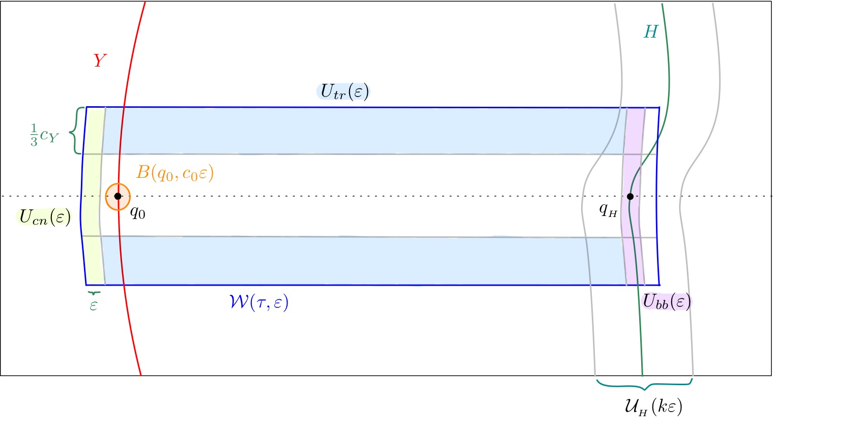
Figure 1.

Finally, we define the cutoff function $\chi_{\varepsilon}\in C^{\infty}_{0}(\mathcal{W}_{{}_{\!Y}}(\tau_{{}_{\!H}},\varepsilon_{{}_{\!Y}}))$ with

$$\chi_{\varepsilon}(y^{\prime},y_{n}):=\chi_{\varepsilon,_{Y}}(y_{n})\cdot\chi_{\varepsilon,_{H}}(y_{n})\cdot\chi_{\varepsilon,tr}(y^{\prime}).$$ (21)

By the Leibniz rule it follows that

$${\operatorname{supp\,}}\,\partial\chi_{\varepsilon}\subset U_{\!cn}(\varepsilon)\cup U_{bb}(\varepsilon)\cup U_{tr}(\varepsilon),$$ (22)

where, as shown in Figure 1,

$$U_{\!cn}(\varepsilon) :={\operatorname{supp\,}}\,\partial\chi_{\varepsilon,_{Y}}\times{\operatorname{supp\,}}\chi_{\varepsilon,tr}\subset\{-2\varepsilon<y_{n}<-\varepsilon,\;|y^{\prime}|<c_{{}_{\!Y}}\}$$

$$U_{bb}(\varepsilon) :={\operatorname{supp\,}}\,\partial\chi_{\varepsilon,_{H}}\times{\operatorname{supp\,}}\,\chi_{\varepsilon,tr}\subset\{|y_{n}-\tau_{{}_{\!H}}|<\varepsilon,\;|y^{\prime}|<c_{{}_{\!Y}}\}$$

$$U_{tr}(\varepsilon) :={\operatorname{supp\,}}(\chi_{\varepsilon,_{Y}}\chi_{\varepsilon,_{H}})\times{\operatorname{supp\,}}\,\partial\chi_{\varepsilon,tr}\subset\{-2\varepsilon<y_{n}<\tau_{{}_{\!H}}+\varepsilon,\;\tfrac{1}{3}c_{{}_{\!Y}}<|y^{\prime}|<c_{{}_{\!Y}}\}.$$

We note that one can refine the containment in (22) slightly by setting

$$\tilde{U}_{tr}(\varepsilon):=U_{tr}(\varepsilon)\setminus\big{(}U_{bb}(\varepsilon)\cup U_{\!cn}(\varepsilon)\big{)},$$

and noting that Leibniz rule actually gives

$${\operatorname{supp\,}}\,\partial\chi_{\varepsilon}\subset\tilde{U}_{tr}(\varepsilon)\cup U_{bb}(\varepsilon)\cup U_{\!cn}(\varepsilon).$$ (23)

2.3. Proof of Theorem 2

Let $q_{0}\in{\operatorname{supp\,}}(\pi_{*}\mu)$, $\tau_{{}_{\!Y}}>0$ be as in Lemma 2.1, and $q_{{}_{\!H}}\in H$ be chosen so that $\tau_{{}_{\!H}}=d(q_{0},q_{{}_{\!H}})=d(K,H).$ We continue to let $Y$ be the geodesic sphere defined in (18) with $(y^{\prime},y_{n}):\mathcal{U}_{{}_{\!Y}}(\tau_{{}_{\!Y}})\to{\mathbb{R}}^{n}$ geodesic normal coordinates adapted to $Y$ as in (19). For $\varepsilon_{{}_{\!Y}}$ satisfying (15) let

$$\mathcal{W}:=\mathcal{W}_{{}_{\!Y}}(\tau_{{}_{\!H}},\varepsilon_{{}_{\!Y}}).$$

After possibly shrinking $\varepsilon_{{}_{\!Y}}>0$ further, depending only on $(H,Y)$, there exists $k>2$ such that for $0<\varepsilon<\varepsilon_{{}_{\!Y}}$ (see Fig 1)

$$\{(y^{\prime},y_{n}):\;\,\,|y_{n}-\tau_{{}_{\!H}}|<\varepsilon,\,\,|y^{\prime}|\leq 4\varepsilon\}\subset\mathcal{U}_{{}_{\!H}}(k\varepsilon).$$ (24)

We also choose $c_{0}>0$ so that for $0<\varepsilon<\varepsilon_{{}_{\!Y}}$ (see Fig 1), the control ball

$$B(q_{0},c_{0}\varepsilon)\subset\{(y^{\prime},y_{n}):\;|(y^{\prime},y_{n})|<\tfrac{1}{5}\varepsilon\},$$ (25)

and continue to assume that (17) holds; that is, $\tau_{{}_{\!H}}+2\varepsilon_{{}_{\!Y}}<\tau_{{}_{\!Y}}$.

We now carry out the Carleman argument. With $\varepsilon$ as in (20) and $\chi_{\varepsilon}\in C^{\infty}_{0}(\mathcal{W})$ as defined in (21), set

$$v_{h}:=\chi_{\varepsilon}e^{\psi/h}u_{h},\qquad\psi(y^{\prime},y_{n})=y_{n}+2\tau_{{}_{\!H}}\rho_{\varepsilon}(y^{\prime}),$$ (26)

with $\psi$ as in (8) with $\tau_{{}_{\!H}}$ in place of $\tau$. By Lemma 8, since $0<\tau_{{}_{\!H}}<\tau_{{}_{\!Y}},$ $\psi\in C^{\infty}(\mathcal{W})$ is a Carleman weight. Thus, by the subelliptic Carleman estimates [Zw, Theorem 7.5], there exists $C>0$ so that, with $P_{\psi}(h)$ as in (9),

$$\|P_{\psi}(h)v_{h}\|^{2}_{{}_{\!L^{2}(\mathcal{W})}}\geq Ch\,\|v_{h}\|_{{}_{\!L^{2}(\mathcal{W})}}^{2}.$$ (27)

Note that $\chi_{\varepsilon}=1$ on $B(q_{0},c_{0}\varepsilon)$ by (25) and $B(q_{0},c_{0}\varepsilon)\subset\mathcal{W}.$ In addition, since $\rho_{\varepsilon}=0$ on $B(q_{0},c_{0}\varepsilon)$, we have

$$\psi(y)=y_{n}\geq-\tfrac{1}{2}\varepsilon,\qquad(y^{\prime},y_{n})\in B(q_{0},c_{0}\varepsilon).$$ (28)

Also, since $q_{0}\in{\operatorname{supp\,}}\!(\pi_{*}\mu),$ it follows that for all $r>0$ there is $C(r)>0$ such that

$$\pi_{*}\mu(B(q_{0},r))\geq C(r)>0.$$

In particular, there exist constants $C(\varepsilon)>0$ and $h_{0}(\varepsilon)>0$ such that for $h\in(0,h_{0}(\varepsilon)],$

$$\int_{B(q_{0},c_{0}\varepsilon)}|u_{h}|^{2}\,dv_{g}\geq C(\varepsilon).$$ (29)

Thus, from (26), (28) and (29) it follows that there exist $C(\varepsilon)>0$ and $h_{0}(\varepsilon)>0$ such that

$$\|v_{h}\|_{L^{2}(\mathcal{W})}^{2}\geq e^{-\varepsilon/h}\int_{B(q_{0},c_{0}\varepsilon)}|u_{h}|^{2}\,dv_{g}\geq C(\varepsilon)e^{-\varepsilon/h},$$ (30)

for $h\in(0,h_{0}(\varepsilon)].$ Here, (30) gives the required lower bound for the RHS in (27).

Next, since $P(h)u_{h}=0,$ we will use that

$$P_{\psi}(h)v_{h}=e^{\psi/h}[P(h),\chi_{\varepsilon}]u_{h}.$$ (31)

Also, since $[P(h),\chi_{\varepsilon}]$ is an $h$-differential operator of order one supported in ${\operatorname{supp\,}}\partial\chi_{\varepsilon}\subset\tilde{U}_{tr}(\varepsilon)\cup U_{bb}(\varepsilon)\cup U_{\!cn}(\varepsilon),$ where the inclusion was derived in (23). Thus, from (27) and (30) it follows that, after possibly shrinking $C(\varepsilon),$

$$\|P_{\psi}(h)v_{h}\|^{2}_{L^{2}(U_{bb}(\varepsilon))}+\|P_{\psi}(h)v_{h}\|^{2}_{L^{2}(U_{\!cn}(\varepsilon))}+\|P_{\psi}(h)v_{h}\|^{2}_{L^{2}(\tilde{U}_{tr}(\varepsilon))}\geq C(\varepsilon)he^{-\varepsilon/h}.$$ (32)

We proceed to find upper bounds for each term in the LHS of (32). On the control set $U_{\!cn}(\varepsilon)$ we have that $-2\varepsilon<y_{n}<-\varepsilon$ and so, since $\rho_{\varepsilon}\leq 0,$

$$\psi(y)\leq y_{n},\qquad y\in U_{\!cn}(\varepsilon).$$ (33)

From (31) and (33), it follows by $L^{2}$-boundedness that there are constants $\tilde{C}>0$ and $\tilde{h}_{0}>0$ such that

$$\|P_{\psi}(h)v_{h}\|^{2}_{L^{2}(U_{\!cn}(\varepsilon))}\leq\|e^{y_{n}/h}[P(h),\chi_{\varepsilon}]u_{h}\|^{2}_{L^{2}(U_{\!cn}(\varepsilon))}\leq\tilde{C}h^{2}e^{-2\varepsilon/h},$$ (34)

for all $0<h<\tilde{h}_{0}$.

On the transition set $\tilde{U}_{tr}(\varepsilon)$ we have $\rho_{\varepsilon}(y^{\prime})=-1$ and so from (20) it follows that

$$\psi(y)=y_{n}+2\tau_{{}_{\!H}}\rho_{\varepsilon}(y^{\prime})=y_{n}-2\tau_{{}_{\!H}}\leq\tau_{{}_{\!H}}+\varepsilon-2\tau_{{}_{\!H}}\leq-\tfrac{9}{10}\tau_{{}_{\!H}}<-9\varepsilon,\,\qquad y\in U_{tr}(\varepsilon).$$

Therefore, after possibly adjusting $\tilde{C}$ and $\tilde{h}_{0}$, and recalling (15) and (31),

$$\|P_{\psi}(h)v_{h}\|^{2}_{L^{2}(U_{tr}(\varepsilon))}\leq\tilde{C}h^{2}e^{-{18}\varepsilon/h},$$ (35)

for all $0<h<\tilde{h}_{0}(\varepsilon)$.

In view of (34) and (35), both the transition and control terms on the LHS of (32) can be absorbed into the RHS for $h>0$ small. The result is that there are constants $C(\varepsilon)>0$ and $h_{0}(\varepsilon)>0$ such that for all $0<h<h_{0}(\varepsilon)$

$$\|e^{\psi/h}[P(h),\chi_{\varepsilon}]u_{h}\|^{2}_{L^{2}(U_{bb}(\varepsilon))}=\|P_{\psi}(h)v_{h}\|^{2}_{L^{2}(U_{bb}(\varepsilon))}\geq C(\varepsilon)he^{-\varepsilon/h}.$$ (36)

Next, on the black-box set ${U}_{bb}(\varepsilon)$ we have $y_{n}<\tau_{{}_{\!H}}+\varepsilon$ and so,

$$\psi(y)\leq\tau_{{}_{\!H}}+\varepsilon,\quad y\in{U}_{bb}(\varepsilon),$$

since $\rho_{\varepsilon}\leq 0.$ So, (36) implies that

$$\tilde{C}h^{2}\|u_{h}\|_{L^{2}(U_{bb}(\varepsilon))}^{2}\geq\|[P(h),\chi_{\varepsilon}]u_{h}\|^{2}_{L^{2}(U_{bb}(\varepsilon))}\geq Che^{-(2\tau_{{}_{\!H}}+3\varepsilon)/h},$$ (37)

for some $\tilde{C}>0$.

From (24), it is clear that for all $0<\varepsilon<\varepsilon_{{}_{\!Y}}$

$$U_{bb}(\varepsilon)\subset\{(y^{\prime},y_{n}):\,\,|y_{n}-\tau_{{}_{\!H}}|<\varepsilon,\,\,|y^{\prime}|\leq 3\varepsilon\}\subset\mathcal{U}_{{}_{\!H}}(k\varepsilon).$$

Then, by (37), there are $C(\varepsilon)>0$ and $h_{0}(\varepsilon)>0$ such that

$$\|u_{h}\|_{L^{2}(\mathcal{U}_{{}_{\!H}}(k\varepsilon))}^{2}\geq C(\varepsilon)h^{-1}e^{-(2\tau_{{}_{\!H}}+3\varepsilon)/h},\qquad 0<h<h_{0}.$$

Since by assumption $k>2,$ we have $\tfrac{3}{2}\varepsilon<k\varepsilon$ and by setting $\tilde{\varepsilon}=k\varepsilon$, it follows that $\|u_{h}\|_{L^{2}(\mathcal{U}_{{}_{\!H}}({\tilde{\varepsilon}}))}\geq Ch^{-{1}/{2}}e^{-(\tau_{{}_{\!H}}+\tilde{\varepsilon})/h}$ for all $0<\tilde{\varepsilon}<k\varepsilon_{0}$ and $0<h<h_{0}$. The theorem then follows since $\tau_{{}_{\!H}}=d(q_{0},H)$. ∎

3. Goodness estimates in lacunary regions: Proof of Theorem 1

In this section, we prove Theorem 1. Before carrying out the proof, we briefly recall some background material.

3.1. Semiclassical pseudodifferential operators (h-pseudos)

Let $U\subset M$ be open. We say that $a\in S^{m}_{h}(U)$ provided $a\sim h^{-m}(a_{0}+ha_{1}+\dots)$ in the sense that for all $\ell\geq 0$

$$\begin{gathered}a-h^{-m}\sum_{0\leq j\leq\ell}h^{j}a_{j}\;\;\in h^{-m+\ell+1}S^{0}(U),\end{gathered}$$ (38)

where (see [Zw, Section 14.2.2])

$$S^{0}(U)=\Big{\{}a\in C^{\infty}(T^{*}U):\;\partial_{x}^{\alpha}\partial_{\xi}^{\beta}a(x,\xi)=O_{\alpha,\beta}(1)\;\text{for all }\,\alpha,\beta\in\mathbb{N}^{n},\,\,(x,\xi)\in T^{*}U\Big{\}}.$$

Consider now the special case where $H\subset M$ is a closed hypersurface and $\mathcal{U}_{{}_{\!H}}(\tau)$ is an open Fermi tube about H of width $\tau>0.$ In the following, we let $x=(x^{\prime},x_{n}):\mathcal{U}_{{}_{\!H}}(\tau)\to{\mathbb{R}}^{n}$ be Fermi coordinates centered on the hypersurface $H=\{x_{n}=0\}.$ We say that that $P(h)$ is an $h$-pseudodifferential operator ($h$-pseudo) on the tube $\mathcal{U}_{{}_{\!H}}(\tau)$ if its kernel can be written in the form

$$P(x,y;h)=K_{a}(x,y;h)+R(x,y;h)$$

where

$$K_{a}(x,y;h)=\frac{1}{(2\pi h)^{m}}\int_{{\mathbb{R}}^{n}}e^{\frac{i}{h}\left\langle x-y,\xi\right\rangle}\tilde{\chi}_{{}_{\!\,1}}(x_{n})\,a(x,\xi;h)\,\tilde{\chi}_{{}_{\!\,2}}(y_{n})d\xi,$$ (39)

and for all $\alpha,\beta\in\mathbb{N}^{n}$,

$$|\partial_{x}^{\alpha}\partial_{y}^{\beta}R(x,y)|={\mathcal{O}}_{\alpha,\beta}(h^{\infty}).$$

Here, $\tilde{\chi}_{{}_{\!\,1}},\tilde{\chi}_{{}_{\!\,2}}\in C^{\infty}_{0}(\mathcal{U}_{{}_{\!H}}(\tau))$ are tubular cutoffs with $\tilde{\chi}_{{}_{\!\,1}}\Subset\tilde{\chi}_{{}_{\!\,2}}$ and $a\in S^{m}_{h}(\mathcal{U}_{{}_{\!H}}(\tau))$. As for the corresponding operator, we write $P(h)\in\Psi^{m}_{h}(\mathcal{U}_{{}_{\!H}}(\tau)).$

In the following it will also be useful to introduce two other cutoffs $\chi_{{}_{\!\,1}},\chi_{{}_{\!\,2}}\in C^{\infty}_{0}(\mathcal{U}_{{}_{\!H}}(\tau))$ with $\chi_{{}_{\!\,2}}\Subset\tilde{\chi_{2}}\Subset\chi_{{}_{\!\,1}}\Subset\tilde{\chi}_{{}_{\!\,1}}.$ For concreteness, choosing $\varepsilon\in(0,\varepsilon_{{}_{\!Y}})$ we assume that

• $\tilde{\chi}_{{}_{\!\,1}}\in C^{\infty}_{0}([-2\varepsilon,2\varepsilon])$ with $\chi_{{}_{\!\,1}}(x_{n})=1$ when $|x_{n}|\leq\varepsilon$,

• $\chi_{{}_{\!\,1}}\in C^{\infty}_{0}([-\varepsilon,\varepsilon])$ with $\chi_{{}_{\!\,1}}(x_{n})=1$ when $|x_{n}|\leq\varepsilon/2$,

• $\tilde{\chi}_{{}_{\!\,2}}\in C^{\infty}_{0}([-\varepsilon/2,\varepsilon/2])$ with $\tilde{\chi}_{{}_{\!\,1}}(x_{n})=1$ when $|x_{n}|\leq\varepsilon/4,$

• $\chi_{{}_{\!\,2}}\in C^{\infty}_{0}((-\varepsilon/4,\varepsilon/4))$ with $\chi_{{}_{\!\,2}}(x_{n})=1$ when $|x_{n}|\leq\varepsilon/8$.

For convenience, in the following we will use Fermi coordinates $x=(x^{\prime},x_{n})$, with $H=\{x_{n}=0\}$, to represent the $h$-pseudo’s without further comment. Given a symbol $a\in S^{m}_{h}(\mathcal{U}_{{}_{\!H}}(\tau))$ we write $a(x,hD_{x})$ for the operator whose kernel is given by (39). In what follows, we will say that $a\in S^{m}_{h}({\mathcal{U}_{{}_{\!H}}(\tau)})$ is a tangential symbol if $a=a(x,\xi^{\prime})$ does not depend on the geodesic conormal variable $\xi_{n}$. In this case we also say that $a(x,hD_{x^{\prime}})$ is a tangential operator.

For future reference, we also recall the following basic definition.

Definition 3.1.

We say that $A\in\Psi_{h}^{m}(\mathcal{U}_{{}_{\!H}}(\tau))$ is $h$-elliptic if there exists $C_{0}>0$ such that the principal symbol $\sigma(A):=a_{0}$ satisfies

$$|a_{0}(x,\xi)|\geq C_{0}h^{-m},\qquad(x,\xi)\in T^{*}(\mathcal{U}_{{}_{\!H}}(\tau)).$$

For more detail on the calculus of h-pseudos, we refer the reader to [Zw, Mar02].

3.2. Operator factorization

In this section we carry out a factorization of an $h$-elliptic pseudo $Q(h)\in\Psi_{h}^{0}(\mathcal{U}_{{}_{\!H}}(\tau))$ over a Fermi tube $\mathcal{U}_{{}_{\!H}}(\tau)$ in terms of the diffusion operator $hD_{x_{n}}-iB(x,hD_{x^{\prime}})$, where $B(x,\xi^{\prime})\gtrapprox 1$ is a tangential symbol.

Proposition 3.2.

Let $\tau\in(0,\tau_{{}_{\!H}}]$, $Q(h)\in\Psi_{h}^{0}(\mathcal{U}_{{}_{\!H}}(\tau))$ be an $h$-elliptic operator and $\chi_{{}_{\!\,1}},\chi_{{}_{\!\,2}}\in C^{\infty}_{0}(\mathcal{U}_{{}_{\!H}}(\tau),[0,1])$ be the tubular cutoffs defined above with $\chi_{{}_{\!\,1}}\Subset\chi_{{}_{\!\,2}}.$ Let $B\in S^{0}({\mathcal{U}_{{}_{\!H}}(\tau)})$ be a real valued tangential symbol and $c_{0}>0$ such that $B(x,\xi^{\prime})\geq c_{0}$ when $(x,\xi)\in T^{*}\mathcal{U}_{{}_{\!H}}(\tau)$.

Then, there exists an $h$-elliptic operator $A(h)\in\Psi_{h}^{0}(\mathcal{U}_{{}_{\!H}}(\tau))$ such that

$$\big{\|}\chi_{{}_{\!\,2}}\,\Big{(}Q(h)-A(h)\,\big{(}hD_{x_{n}}-iB(x,hD_{x^{\prime}})\big{)}\,\Big{)}\,\chi_{{}_{\!\,1}}\big{\|}_{{}_{\!L^{2}\to L^{2}}}={{\mathcal{O}}(h^{\infty})}.$$ (40)

Proof.

Let $q\sim\sum_{j=0}^{\infty}q_{-j}h^{j}$ be the symbol of $Q(h).$ First, note that

$$|\xi_{n}-iB(x,\xi^{\prime})|^{2}=\xi_{n}^{2}+|B(x,\xi^{\prime})|^{2}\geq c_{0}^{2},\quad(x,\xi)\in T^{*}\mathcal{U}_{{}_{\!H}}(\tau),$$

and since by assumption $Q(h)$ is $h$-elliptic, we have that

$$a_{0}(x,\xi):=\frac{q_{0}(x,\xi)}{\xi_{n}-iB(x,\xi^{\prime})}\in S^{0}(T^{*}\mathcal{U}_{{}_{\!H}}(\tau)),\qquad a_{0}(x,\xi)\geq C>0.$$

Our objective is to obtain an operator factorization of the form

$$\chi_{{}_{\!\,2}}Q(h)\chi_{{}_{\!\,1}}=\chi_{{}_{\!\,2}}A(x,hD_{x})\,\big{(}hD_{x_{n}}-iB(x,hD_{x}^{\prime})\big{)}\chi_{{}_{\!\,1}}+R(h),$$

$$\|R(h)\|_{L^{2}\to L^{2}}={\mathcal{O}}(h^{\infty}).$$ (41)

To achieve (41), our ansatz is to use the factorization at the level of principal symbols

$$q_{0}(x,\xi)=a_{0}(x,\xi)(\xi_{n}-iB(x,\xi^{\prime})),$$ (42)

to iteratively construct an $h$-smooth symbol $a\in S^{0}_{h}(T^{*}\mathcal{U}_{{}_{\!H}}(\tau))$ satisfying

$$q(x,\xi,h)\sim a(x,\xi,h)\,\#\Big{(}\xi_{n}-iB(x,\xi^{\prime})\Big{)},$$ (43)

where $q\sim\sum_{j=0}^{\infty}q_{-j}h^{j}$ is the total symbol of $Q(h).$ Since the elliptic symbol $\xi_{n}-iB(x,\xi^{\prime})$ is already in the desired form, we perturb the $a_{0}$-term only by adding lower order corrections in $h$ to match the total symbol of $q_{0}$. The first term $a_{0}$ already satisfies the desired equation in (43):

$$q_{0}=a_{0}(\xi_{n}-iB),\qquad a_{0}\in{S^{0}(\mathcal{U}_{{}_{\!H}}(\tau))}.$$

For the second term $a_{-1}$ one must solve an equation of the form

$$q_{-1}=a_{-1}(\xi_{n}-iB)+r_{-1},$$ (44)

where $r_{-1}=-\partial_{\xi}a_{0}\cdot\partial_{x}B:=-\sum_{j=1}^{n}\partial_{\xi_{j}}a_{0}\,\partial_{x_{j}}B\in S^{0}(\mathcal{U}_{{}_{\!H}}(\tau))$. Since $\xi_{n}-iB\neq 0,$ we just solve for $a_{-1}$ in (44) and get

$$a_{-1}=(\xi_{n}-iB)^{-1}\,(q_{-1}-r_{-1})=(\xi_{n}-iB)^{-1}\,(q_{-1}+\partial_{\xi}a_{0}\partial_{x}B),$$ (45)

where we note that $a_{-1}\in S^{0}(T^{*}\mathcal{U}_{{}_{\!H}}(\tau)).$ For the subsequent terms $a_{-m}$ with $m\geq 2,$ we have

$$a_{-m}:=(\xi_{n}-iB)^{-1}{\Big{(}q_{-m}+i\sum_{1\leq\ell\leq m}(-i)^{\ell}\sum_{|\alpha|=\ell}\frac{1}{\alpha!}(\partial_{\xi}^{\alpha}a_{\ell-m}\,\partial_{x}^{\alpha}B)}\Big{)}.$$ (46)

It follows that the decomposition (43) holds for

$$a\sim\sum_{j=0}^{\infty}a_{-j}h^{j}\in S_{h}^{0}(\mathcal{U}_{{}_{\!H}}(\tau)).$$

Setting $A(h):=a(x,hD_{x})$ and noting $hD_{x_{n}}=Op_{h}(\xi_{n})$, it follows that the remainder

$$R(h):=\chi_{{}_{\!\,2}}\,\big{(}\,Q(h)-A(h)(hD_{x_{n}}-iB(x,hD_{x^{\prime}})\,\big{)}\,\chi_{{}_{\!\,1}}$$

satisfies $\|R(h)\|_{L^{2}\to L^{2}}=O(h^{\infty}).$ ∎

Remark 3.3.

Since $Q(h)$ is $h$-elliptic in the Fermi tube about $H$, the factorization in Proposition 3.2 is by no means unique; indeed, one can factorize $Q$ over the Fermi tube in terms of any reference $h$-elliptic operator. As we will see in Proposition 3.4, the factorization corresponding to the specific choice of the reference diffusion operator $hD_{n}-iB_{0}$, where $B_{0}>0$ is constant, is particularly convenient in converting the lower bound for $L^{2}$ eigenfunction mass $\|u_{h}\|_{{}_{\!\mathcal{U}_{H}(\varepsilon)}}^{2}$ into an actual lower bound for the $L^{2}$ restrictions, $\|\gamma_{{}_{\!H}}u_{h}\|_{L^{2}(H)}$

3.3. Exploiting the lacunary condition

In this section, we explain how to combine Proposition 3.2 with the lacunary condition on $Q(h)$ for the eigenfunction sequence $\{u_{h}\}$ to essentially allow us to work as if $(hD_{x_{n}}-iB_{0})u_{h}=O(e^{-C/h})$ on $\mathcal{U}_{{}_{\!H}}(\varepsilon)$, where $B_{0}$ is a positive constant.

In the following, it will be useful to define truncated cutoff functions. Given any cutoff $\chi\in C^{\infty}_{0}(\varepsilon),$ we set

$$\chi^{+}:=\chi\cdot{\bf 1}_{x_{n}\geq 0},\qquad\mathcal{U}_{{}_{\!H}}^{+}(\varepsilon):=\{x\in\mathcal{U}_{{}_{\!H}}(\varepsilon),\,x_{n}\geq 0\}.$$

In addition, given an open submanifold $\tilde{H}\subset H$ and $\varepsilon>0$ sufficiently small, we let $\psi(x^{\prime})\in C^{\infty}_{0}(\tilde{H};[0,1])$ with the property that there exists a proper open submanifold $\tilde{H}_{\varepsilon}\subset\tilde{H}$ with $\max_{x\in\tilde{H}}d(\tilde{H}_{\varepsilon},x)<\varepsilon$ such that

$$\psi|_{\tilde{H}_{\varepsilon}}=1.$$ (47)

Finally, in the following, $\gamma_{{}_{\!H}}:M\to H$ denotes the restriction operator to $H$.

The proof of Theorem 1 hinges on the following factorization result.

Proposition 3.4.

Let $\{u_{h}\}$ be a sequence of eigenfunctions satisfying (1), $H\subset M$ be a closed $C^{\infty}$-hypersurface, and suppose there exists an $H$-lacunary region for $\{u_{h}\}$ containing the Fermi tube $\mathcal{U}_{{}_{\!H}}(2\varepsilon)$. Then, if $B_{0}>0$ is any positive constant, $\tilde{H}\subset H$ is any open submanifold of $H$ and $\psi\in C^{\infty}_{0}(\tilde{H})$ is a tangential cutoff satisfying (47), there exist operators $E(h):C_{0}^{\infty}(\mathcal{U}_{{}_{\!H}}(\varepsilon))\to C^{\infty}(\mathcal{U}_{{}_{\!H}}^{+}(\varepsilon))$ such that for some $C>0$,

$$\big{\|}\chi_{{}_{\!\,2}}^{+}\,\big{(}hD_{x_{n}}-iB_{0}\big{)}\,\psi\big{(}I+E(h)\big{)}\,\chi_{{}_{\!\,1}}u_{h}\big{\|}_{{}_{\!L^{2}}}=O(e^{-C/h}),$$ (48)

where $\|\chi_{{}_{\!\,2}}^{+}E(h)\chi_{{}_{\!\,1}}\|_{L^{2}\to L^{2}}=O(h^{\infty})$ and $\gamma_{{}_{\!H}}E(h)=0.$

Proof.

We apply Proposition 3.2 with $B(x,\xi^{\prime}):=B_{0},$ so that $B(x^{\prime},hD_{x^{\prime}})=B_{0}\,I$ is simply the multiplication operator by $B_{0}>0.$

Since the operator $A(h)\in\Psi^{0}_{h}(\mathcal{U}_{{}_{\!H}}(2\varepsilon))$ from Proposition 3.2 is $h$-elliptic over $\mathcal{U}_{{}_{\!H}}(2\varepsilon)$, there exists a local parametrix $L(h)\in{\Psi_{h}^{0}(\mathcal{U}_{{}_{\!H}}(2\varepsilon))}$ such that

$$\|\chi_{{}_{\!\,1}}\big{(}\,L(h)A(h)-I\,\big{)}\chi_{{}_{\!\,1}}\|_{L^{2}\to L^{2}}=O(h^{\infty}).$$ (49)

Since $Q(h)$ is lacunary for $u_{h}$, there exists $C>0$, depending only on $\{u_{h}\}$, such that

$$\|\chi_{{}_{\!\,2}}Q(h)\chi_{{}_{\!\,1}}u_{h}\|_{L^{2}}=O(e^{-C/h}).$$

Therefore, since $\|\chi_{{}_{\!\,1}}[L(h),\chi_{{}_{\!\,2}}]\|_{L^{2}\to{L^{2}}}=O(h^{\infty}),$ it follows from Proposition 3.2 (49) that

$$\chi_{{}_{\!\,2}}\big{(}hD_{x_{n}}-iB(x,hD_{x^{\prime}})\big{)}\chi_{{}_{\!\,1}}u_{h}=\chi_{{}_{\!\,2}}R^{\prime}(h)\chi_{{}_{\!\,1}}u_{h}+O(e^{-C/h}),$$ (50)

where

$$\|\chi_{{}_{\!\,2}}R^{\prime}(h)\chi_{{}_{\!\,1}}\|_{L^{2}\to L^{2}}=O(h^{\infty}).$$ (51)

It follows from (50) that

$$\chi_{{}_{\!\,2}}^{+}\psi\big{(}hD_{x_{n}}-iB_{0}\big{)}\chi_{{}_{\!\,1}}u_{h}=\chi_{{}_{\!\,2}}^{+}\psi R^{\prime}(h)\chi_{{}_{\!\,1}}u_{h}+O(e^{-C/h}).$$ (52)

Moreover, by variation of constants, with $E(h):C_{0}^{\infty}(\mathcal{U}_{{}_{\!H}}(\varepsilon))\to C^{\infty}(\mathcal{U}_{{}_{\!H}}^{+}(\varepsilon))$ given by

$$E(h)f(x^{\prime},x_{n})=-\frac{i}{h}\int_{0}^{x_{n}}e^{-(x_{n}-\tau)B_{0}/h}\,R^{\prime}(h)f(x^{\prime},\tau)\,d\tau,\quad x_{n}\in[0,\varepsilon],$$ (53)

we obtain that $\gamma_{{}_{\!H}}E(h)=0$ and

$$\big{(}hD_{x_{n}}-iB_{0}\big{)}E(h)\chi_{{}_{\!\,1}}=-R^{\prime}(h)\chi_{{}_{\!\,1}},\quad x_{n}\in[0,\varepsilon].$$ (54)

Thus, from (52) it follows that

$$\chi_{{}_{\!\,2}}^{+}\psi\big{(}hD_{x_{n}}-iB_{0}\big{)}\chi_{{}_{\!\,1}}u_{h}=-\chi_{{}_{\!\,2}}^{+}\psi\big{(}hD_{x_{n}}-iB_{0}\big{)}E(h)\chi_{{}_{\!\,1}}u_{h}+O(e^{-C/h}).$$ (55)

Since

$${[hD_{x_{n}}-iB_{0},\psi]=0,}$$ (56)

the bound in (48) follows from (55). Also, by (51) and the fact that $B_{0}>0$,

$$\|E(h)\|_{L^{2}(\mathcal{U}_{{}_{\!H}}(\varepsilon))\to L^{2}(\mathcal{U}_{{}_{\!H}}^{+}(\varepsilon))}=O(h^{\infty}).$$

∎

Remark 3.5.

We note that the final crucial step in the proof of Proposition 3.4 involves showing that the error term $R^{\prime}(h)$ in (51) can also be factorized as in (52). Proposition 3.4 implies that $(hD_{x_{n}}-iB_{0}\big{)}v_{h}=O(e^{-C/h})$ with $v_{h}=\psi(I+E(h))\chi_{{}_{\!\,1}}u_{h}$, where we note that $v_{h}=\psi u_{h}$ on $H$ since $\gamma_{{}_{\!H}}E(h)=0$. We will also use that the $L^{2}$-mass of $v_{h}$ is comparable to that of $\psi u_{h}$ since $\|\chi_{{}_{\!\,2}}^{+}E(h)\chi_{{}_{\!\,1}}\|_{L^{\infty}\to L^{\infty}}=O(h^{\infty})$.

Remark 3.6.

A key step in the proof of Proposition 3.4 that allows us to localize the eigenfunction restriction bounds to an open submanifold $\tilde{H}\subset H$ involves the commutator condition $[hD_{x_{n}}-iB(x,hD_{x^{\prime}}),\psi]=0$ in (56) where $\psi=\psi(x^{\prime})\in C^{\infty}_{0}(\tilde{H})$ is a tangential cutoff satisfying (47). Since trivially $[hD_{x_{n}},\psi]=0,$ (56) is equivalent to $[B(x,hD^{\prime}),\psi]=0$ and the latter requirement forces us to choose the tangential $h$-psdo to be a constant multiplication operator; that is, $B(x,hD^{\prime})=B_{0}$ with $B_{0}>0.$

3.4. Proof of Theorem 1

Let $\tilde{H}\subset H$ be an open submanifold and choose $q_{0}\in K={\operatorname{supp\,}}\!(\pi_{*}\mu)$ and $q_{{}_{\!H}}\in\tilde{H}$ so that

$$0<d(q_{0},q_{{}_{\!H}})=d(K,\tilde{H})<\tau_{0},$$

where $\tau_{0}$ is as in Theorem 2.

In the following we let $(x^{\prime},x_{n})$ be Fermi coordinates adapted to $H$,

$$H=\{x_{n}=0\},\qquad q_{{}_{\!H}}=(0,0),$$

and we assume they are well defined for $(x^{\prime},x_{n})\in\mathcal{U}_{{}_{\!H}}(2\varepsilon).$

We continue to let $\chi_{j}\in C^{\infty}_{0}(\mathcal{U}_{{}_{\!H}}(2\varepsilon))$, for $j=1,2,$ be the nested cutoff functions in Section 3.3. In general, for each $0\leq\tau<2\varepsilon$ we define the level hypersurface

$$H_{\tau}:=\{(x^{\prime},x_{n}):\;x_{n}=\tau\},\qquad H_{0}=H.$$

We note that for $0<x_{n}<2\varepsilon$ there is a natural diffeomorphism $\kappa_{\tau}:H\to H_{x_{n}}$ that in Fermi coordinates takes the form $\kappa_{\tau}(x^{\prime})=(x^{\prime},\tau).$ Consequently, using $\kappa_{\tau}$ to parametrize $H_{x_{n}}$ by $H$ together with the fact that $({\kappa_{\tau}})_{*}(d\sigma_{{}_{\!\!H}})=d\sigma_{{}_{\!\!H_{\tau}}}$, for every $v\in L^{2}(\mathcal{U}_{{}_{\!H}}(2\varepsilon))$

$$\|\gamma_{{}_{\!H_{\tau}}}v\|_{{}_{\!L^{2}(H_{\tau})}}^{2}=\int_{H}|v(x^{\prime},\tau)|^{2}\,d\sigma_{{}_{\!H}}(x^{\prime})=\|\kappa_{\tau}^{*}\gamma_{{}_{\!H_{\tau}}}v\|^{2}_{{}_{\!L^{2}(H)}}.$$ (57)

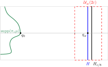
Figure 2.

Let $\psi\in C^{\infty}_{0}(\tilde{H})$ be a tangential cutoff satisfying (47) and $E(h):C_{0}^{\infty}(\mathcal{U}_{{}_{\!H}}(\varepsilon))\to C^{\infty}(\mathcal{U}_{{}_{\!H}}^{+}(\varepsilon))$ as in Proposition 3.4. Set

$$v_{h}:=\psi(I+E(h))\chi_{{}_{\!\,1}}u_{h},\qquad{on}\;\;\mathcal{U}_{{}_{\!H}}^{+}(2\varepsilon)\cap\text{supp}\,\psi,$$

where we note that since $\gamma_{{}_{\!H}}\psi E(h)\chi_{{}_{\!\,1}}u=\psi\gamma_{{}_{\!H}}E(h)\chi_{{}_{\!\,1}}u=0$ and $\chi_{{}_{\!\,1}}|_{H}=1$, it follows that

$$\gamma_{{}_{\!H}}v_{h}=\gamma_{{}_{\!H}}\psi\chi_{{}_{\!\,1}}u_{h}=\psi\gamma_{{}_{\!H}}\chi_{{}_{\!\,1}}u_{h}=\psi\gamma_{{}_{\!H}}u_{h}.$$

Note that from Proposition 3.4, there is $C>0$ depending only on $\{u_{h}\}$ such that

$$\big{\|}\chi_{{}_{\!\,2}}^{+}\,\big{(}hD_{x_{n}}-iB_{0}\big{)}v_{h}\big{\|}_{{}_{\!{L^{2}}}}=O(e^{-C/h}).$$

Since $\chi_{{}_{\!\,2}}^{+}(x_{n})=1$ for $x_{n}\in[0,\frac{\varepsilon}{8}]$, it follows that

$$\tfrac{1}{2}h\partial_{x_{n}}\int_{H}|v_{h}(x^{\prime},x_{n})|^{2}d\sigma_{{}_{\!H}}(x^{\prime})=-\int_{H}B_{0}v_{h}(x^{\prime},x_{n})\overline{v_{h}(x^{\prime},x_{n})}\,d\sigma_{{}_{\!H}}(x^{\prime})+O(e^{-\tilde{C}/h}).$$ (58)

In view of (57) one can rewrite (58) in the form

$$\tfrac{1}{2}h\partial_{x_{n}}\,\|\gamma_{{}_{\!H_{x_{n}}}}v_{h}\|_{L^{2}(H_{x_{n}})}^{2}=-B_{0}\|\gamma_{{}_{\!H_{x_{n}}}}v_{h}\|^{2}_{L^{2}(H_{x_{n}})}+O(e^{-\tilde{C}/h}),\qquad x_{n}\in[0,\tfrac{\varepsilon}{8}].$$ (59)

Integration of (59) over $0\leq x_{n}\leq\frac{\varepsilon}{8}$ and multiplication by $-1$ gives

$${h}\|\gamma_{{}_{\!H}}v_{h}\|_{{}_{\!L^{2}(H)}}^{2}-{h}\|\gamma_{{}_{\!H_{\varepsilon/8}}}v_{h}\|_{{}_{\!L^{2}(H_{\varepsilon/8})}}^{2}=2B_{0}\big{\|}v_{h}\big{\|}_{{}_{\!L^{2}(\mathcal{U}_{{}_{\!H}}(\varepsilon/8))}}^{2}+O(e^{-\tilde{C}/h}),$$ (60)

and consequently,

$${h}\|\gamma_{{}_{\!H}}v_{h}\|_{{}_{\!L^{2}(H)}}^{2}\geq 2B_{0}\big{\|}v_{h}\big{\|}_{{}_{\!L^{2}(\mathcal{U}_{{}_{\!H}}(\varepsilon/8))}}^{2}+O(e^{-\tilde{C}/h}).$$ (61)

We also note that, by Proposition 3.4, we have $\|\chi_{{}_{\!\,2}}^{+}E(h)\chi_{{}_{\!\,1}}\|_{L^{2}\to L^{2}}=O(h^{\infty})$ and so,

$$\big{\|}v_{h}\big{\|}_{{}_{\!L^{2}(\mathcal{U}_{{}_{\!H}}(\varepsilon/8))}}=(1+O(h^{\infty}))\,\big{\|}\psi u_{h}\big{\|}_{{}_{\!L^{2}(\mathcal{U}_{{}_{\!H}}(\varepsilon/8))}}\geq\tfrac{1}{2}\big{\|}\psi u_{h}\big{\|}_{{}_{\!L^{2}(\mathcal{U}_{{}_{\!H}}(\varepsilon/8))}}.$$

Since $\psi|_{\tilde{H}_{\varepsilon}}=1$ on the open submanifold $\tilde{H}_{\varepsilon}\subset\tilde{H}$ with $\max_{x\in\tilde{H}}d(\tilde{H}_{\varepsilon},x)<\varepsilon$ (see (47)), it follows that

$$\big{\|}v_{h}\big{\|}_{{}_{\!L^{2}(\mathcal{U}_{{}_{\!H}}(\varepsilon/8))}}^{2}\geq\tfrac{1}{4}\,\big{\|}u_{h}\big{\|}_{{}_{\!L^{2}(\mathcal{U}_{{}_{\!\tilde{H}_{\varepsilon}}}(\varepsilon/8))}}^{2}.$$ (62)

We next find a lower bound for the RHS of (62) by applying Theorem 2. Indeed, Theorem 2 yields that for $\varepsilon>0$ arbitrarily small, we have

$$\big{\|}v_{h}\big{\|}_{{}_{\!L^{2}(\mathcal{U}_{{}_{\!H}}(\varepsilon/8))}}^{2}\geq\tfrac{1}{2}\,\big{\|}u_{h}\big{\|}_{{}_{\!L^{2}(\mathcal{U}_{{}_{\!\tilde{H}_{\varepsilon}}}(\varepsilon/8))}}^{2}\geq C_{\varepsilon}e^{-{2\,(d(\tilde{H_{\varepsilon}},K)+\varepsilon)/}{h}}\geq C_{\varepsilon}e^{-{2\,(d(\tilde{H},K)+2\varepsilon)/}{h}}.$$ (63)

In the last estimate in (63), we use (47) and the fact that $\max_{x\in\tilde{H}}d(\tilde{H}_{\varepsilon},x)<\varepsilon$ where $\varepsilon>0$ is arbitrarily small but fixed independent of $h$.

Combining (61) and (63), and recalling that $\gamma_{{}_{\!H}}v_{h}=\psi\gamma_{{}_{\!H}}u_{h}$, implies that for any $\varepsilon>0$ and $h\in(0,h_{0}(\varepsilon)]$ there are constants $C_{\varepsilon}>0$ and $C_{\varepsilon}^{\prime}>0$ such that

$$h\|\psi\gamma_{{}_{\!H}}u_{h}\|_{{}_{\!L^{2}(H)}}^{2} \geq C_{\varepsilon}e^{{-2(d(\tilde{H},K)+2\varepsilon)/}{h}}-C_{\varepsilon}^{\prime}e^{-\tilde{C}/h}.$$ (64)

To complete the proof of Theorem 1, we note that, since the second term on the RHS of (64) depends only on the eigenfunction sequence (and not on ${\tilde{H}}$), it is clear that it can be absorbed in the first term provided one chooses $\tilde{H}$ sufficiently close to $K$, with $2\,d(\tilde{H},K)<\tilde{C}.$ Thus, for such $\tilde{H}$ it follows from (64), and the fact that $\psi\in C^{\infty}_{0}(\tilde{H})$, that

$$h\int_{\tilde{H}}|u_{h}|^{2}\,d\sigma_{{}_{\!\tilde{H}}}\geq C_{\varepsilon}^{\prime}e^{{-2(d(\tilde{H},K)+2\varepsilon)/}{h}}.$$

Since $\varepsilon>0$ is arbitrarily small, this concludes the proof of Theorem 1. ∎

4. The case of Schrödinger operators

Let $(M,g)$ be a compact $C^{\infty}$ Riemannian manifold, $V\in C^{\infty}(M,{\mathbb{R}})$. Consider the classical Schrödinger operator

$$P(h)=-h^{2}\Delta_{g}+V-E,$$

where $E$ is a regular value for $V.$ In the classically forbidden region $\{V>E\},$ the eigenfunctions $u_{h}$ satisfy the Agmon-Lithner estimates [Zw]: for all $\delta>0$ there is $C(\delta)>0$ such that

$$|u_{h}(x)|\leq C(\delta)e^{-[d_{E}(x)-\delta]/h},\qquad x\in\{V>E\},$$ (65)

where $d_{E}(x)$ is the distance from $x$ to $\{V=E\}$ in the Agmon metric $g_{E}=(V-E)_{+}|dx|^{2}.$ As a immediate consequence of (65), it follows that if $\mu$ is a defect measure associated to a sequence $\{u_{h}\}$ of $L^{2}$-normalized Schrödinger eigenfunctions, $P(h)u_{h}=0$, then its support is localized in the allowable region; that is,

$${\operatorname{supp\,}}\!(\pi_{*}\mu)\subset\{x\in M:\;V(x)\leq E\}.$$ (66)

We show that if $H$ lies inside the forbidden region $\{V>E\}$ but it is such that a Fermi neighborhood of it reaches the support ${\operatorname{supp\,}}\!(\pi_{*}\mu)$, then $H$ is a good curve for $\{u_{h}\}$ in the sense of (2).

The proof of Theorem 3 follows the same outline as in the homogeneous case in Theorem 1. Here, we explain the relatively minor changes required to prove the analogue of the Carleman estimates in Theorem 2 and refer to the previous sections for further details.

Theorem 4.

Let $(M,g)$ be a compact $C^{\infty}$ Riemannian manifold. Let $\{u_{h}\}$ be a sequence of eigenfunctions satisfying (4) and let $\mu$ be a defect measure associated to it. Let $H\subset M$ be a $C^{\infty}$-hypersurface (possibly with boundary $\partial H$) and suppose there exist $q_{0}\in{\operatorname{supp\,}}\!(\pi_{*}\mu)$ and $q_{{}_{\!H}}\in H\backslash\partial H$ such that $d(q_{0},q_{{}_{\!H}})=d(q_{0},H)$.

For all $\beta>\max_{x\in M}|V(x)-E|^{1/2}$ there exists $\tau_{0}>0$ such that if

$$0<d(q_{0},H)<\tau_{0},$$

then there are constants $C_{0}>0$ and $h_{0}>0$ such that

$$\|u_{h}\|_{{}_{\!L^{2}(\mathcal{U}_{{}_{\!H}}^{\varepsilon})}}\geq C_{0}e^{-\beta d(q_{0},H)/h}$$

for all $h\in(0,h_{0}].$

Proof.

To prove the Carleman analogue of Theorem 2, we need to adapt the argument slightly by constructing a modified weight function. Let

$$\beta^{2}>\max_{y\in M}|V(y)-E|,\qquad\delta_{0}:=\beta^{2}-\max_{y\in M}|V(y)-E|.$$

Given a geodesic sphere $Y_{q,r}:=\partial B(q,r)$, let $a_{{}_{\!\,Y_{q,r}}}$ be the quadratic form dual to the induced metric on $Y_{q,r}$ and $b_{{}_{\!\,Y_{q,r}}}$ be the quadratic form dual to the second fundamental form for $Y_{q,r}$. In particular, for all $y^{\prime}\in Y_{q,r}$, the eigenvalues of $b_{{}_{\!\,Y_{q,r}}}(y^{\prime})$ with respect to $a_{{}_{\!\,Y_{q,r}}}(y^{\prime})$ are the principal curvatures of $Y_{q,r}$ and are are strictly positive. Since the principal curvature of $Y_{q,r}$ grows to infinity as $r\to 0^{+}$, there exists $r_{0}>0$ such that

$$\min_{q\in M}\min_{r\leq r_{0}}\min_{y^{\prime}\in Y_{q,r}}\{2b_{{}_{\!\,Y_{q,r}}}(y^{\prime},\xi^{\prime}):\;a_{{}_{\!\,Y_{q,r}}}(y^{\prime},\xi^{\prime})\geq\tfrac{1}{2}\delta_{0}\}>\max_{y\in M}|\nabla V(y)|.$$ (67)

Condition (67) implies that the principal curvatures of any geodesic sphere $Y_{q,r}$ with $0<r\leq r_{0}$ are bounded below by $\tfrac{1}{2}\max_{y\in M}|\nabla V(y)|$. This will be used to prove that $\psi$ as defined below is a Carleman weight.

Next, let $q_{0}\in{\operatorname{supp\,}}\!(\pi_{*}\mu)$. Let $r_{q_{0}}$ be the maximal radius for which the exponential map $\exp_{q_{0}}$ is a diffeomorphism on $B(q_{0},2r_{q_{0}})$. Let $s_{q_{0}}=\min\{r_{q_{0}},r_{0}\}$ and work with $\tau_{0}<\tfrac{1}{4}s_{q_{0}}$ to be chosen later. Then, let $H\subset M$ be a $C^{\infty}$-hypersurface and $q_{{}_{\!H}}\in H\backslash\partial H$ such that

$$\tau_{{}_{\!H}}:=d(q_{0},q_{{}_{\!H}})=d(q_{0},H),\qquad 0<\tau_{{}_{\!H}}<\tau_{0}.$$ (68)

Let $\gamma$ be a unit speed geodesic joining $q_{0}=\gamma(0)$ with $q_{{}_{\!H}}=\gamma(\tau_{{}_{\!H}})$. Let $q=\gamma(s_{q_{0}})$ and set $Y:=\partial B(q,s_{q_{0}}).$ As before, we work with $(y^{\prime},y_{n})$ being geodesic normal coordinates adapted to $Y$, in which $Y=\{y_{n}=0\},$ and $q_{0}=(0,0),$ and with $\{y_{n}>0\}$ corresponding to points in the interior of $B(q,s_{q_{0}})$.

Note that these coordinates are well defined for $|y_{n}|<2\tau_{{}_{\!Y}}:=s_{q_{0}}$ and $|y^{\prime}|<c_{{}_{\!Y}}$ for some $c_{{}_{\!Y}}>0$, since $\exp_{q}$ is a diffeomorphism on $B(q,2r_{q_{0}})\supset B(q,2s_{q_{0}})$. Furthermore, since $\tau_{0}<\tfrac{1}{4}s_{q_{0}}$, by (68) we also have $\tau_{{}_{\!H}}<\tau_{0}<\tau_{{}_{\!Y}}$. In particular, with $\varepsilon_{{}_{\!Y}}$ as in (15), the Fermi coordinates with respect to $Y$ are well defined on $\mathcal{W}_{{}_{\!Y}}(\tau_{{}_{\!H}},\varepsilon_{{}_{\!Y}})$ as in (6).

In analogy with (8) and (26), for $\varepsilon>0$ we set

$$\psi(y^{\prime},y_{n}):=\beta y_{n}+2\tau_{{}_{\!H}}\rho_{\varepsilon}(y^{\prime}).$$ (69)

Note that, as in (12),

$$p(y,\xi)=\xi_{n}^{2}+a_{{}_{\!\,Y}}(y^{\prime},\xi^{\prime})-2y_{n}b_{{}_{\!\,Y}}(y^{\prime},\xi^{\prime})+R(y,\xi^{\prime})+V(y)-E,$$ (70)

with $R(y,\xi^{\prime})=O(y_{n}^{2}|\xi^{\prime}|^{2})$. Next, note that provided $|y_{n}|\leq\tau_{0},$

$${\operatorname{Re}\,}p_{\psi}=\xi_{n}^{2}+a_{{}_{\!\,Y}}(y^{\prime},\xi^{\prime})-2y_{n}b_{{}_{\!\,Y}}(y^{\prime},\xi^{\prime})+V(y)-E-\beta^{2}+O(\tau_{0}^{2}|\xi^{\prime}|^{2}),$$

$${\operatorname{Im}\,}p_{\psi}=2\beta\xi_{n}+O(\tau_{0}|\xi^{\prime}|).\hskip 202.35622pt$$ (71)

Therefore,

$$\{p_{\psi}=0\}\!\!=\!\!\big{\{}(y,\xi)\in T^{*}(\mathcal{W}_{{}_{\!Y}}(\tau_{{}_{\!H}},\varepsilon_{{}_{\!Y}})):a_{{}_{\!\,Y}}(y^{\prime},\xi^{\prime})=\beta^{2}+E-\!V(y)+O(\tau_{0}),\,\xi_{n}=O(\tau_{0})\big{\}},$$

and so

$$\{{\operatorname{Re}\,}p_{\psi},{\operatorname{Im}\,}p_{\psi}\}(y,\xi) =4{\beta}b_{{}_{\!\,Y}}(y^{\prime},\xi^{\prime}){-2\beta}\partial_{y_{n}}V(y)+O(\tau_{0}),\quad(y,\xi)\in\{p_{\psi}=0\}.$$ (72)

Next, let $\tau_{0}$ be small enough so that on $\{p_{\psi}=0\}$ we have $a_{{}_{\!\,Y}}(y^{\prime},\xi^{\prime})\geq\tfrac{1}{2}\delta_{0}$. Then, the lower bound in (67) together with (72) yield $\{{\operatorname{Re}\,}p_{\psi},{\operatorname{Im}\,}p_{\psi}\}(y,\xi)>0$ on $\{p_{\psi}=0\}$. This shows that $\psi$ is a Carleman weight on $\mathcal{W}_{{}_{\!Y}}(\tau_{{}_{\!H}},\varepsilon_{{}_{\!Y}})$.

One then proceeds exactly as in the proof of Theorem 2 to show that

$$\|u_{h}\|_{L^{2}(\mathcal{U}_{H}(\varepsilon))}\geq C(\varepsilon)e^{-(\beta d(q_{0},H)+\varepsilon)/h}.$$ (73)

∎

The proof of Theorem 4 then follows exactly as for Theorem 2 after noting the following. Let $\{u_{h}\}$ be a sequence of $L^{2}$-normalized eigenfunctions of a Schrödinger operator $P(h)=-h^{2}\Delta_{g}+V-E$. Choose $0<\tau_{1}<\tau_{0}$ such that

$$\mathcal{U}_{{}_{\!H}}(\tau_{1})\subset\{x\in M:\;V(x)>E\}.$$

We recall that in this case, by (66), $K={\operatorname{supp\,}}(\pi_{*}\mu)\subset\{V\leq E\}.$ Since $P(h)$ is elliptic on $\mathcal{U}_{{}_{\!H}}(\tau_{1})$, it has a left parametrix $L(h)$. Thus,

$$Q(h):=L(h)P(h)\in\Psi^{0}_{h}(\mathcal{U}_{{}_{\!H}}(\tau_{1}))$$

is $h$-elliptic over the set $\{V>E\}$ and $Q(h)u_{h}=0$ since the $u_{h}$ are eigenfunctions. We conclude from Remark 1.2 that $Q(h)$ is a lacunary operator for $\{u_{h}\}$.

5. Examples

In this section we present several examples to which our results apply.

5.1. Warped products

Let $(M,g_{{}_{\!M}})$ and $(N,g_{{}_{\!N}})$ be two compact $C^{\infty}$ Riemannian manifolds. We work on the warp product manifold $M\times_{f}N$ endowed with the metric $g=g_{{}_{\!M}}\oplus f^{2}g_{{}_{\!N}}$, for some function $f\in C^{\infty}(M,{\mathbb{R}}\backslash\{0\})$.

Let $\{\varphi_{h}\}_{h}\in C^{\infty}(N)$ be a sequence of normalized eigenfunctions

$$-h^{2}\Delta_{g_{{}_{\!N}}}\varphi_{h}=\varphi_{h},\qquad\|\varphi_{h}\|_{{}_{\!L^{2}(N)}}=1,$$ (74)

and for each $\varphi_{h}$ consider the subspace

$$\mathcal{F}_{h}=\{v\otimes\varphi_{h}:\;v\in L^{2}(M)\}\subset L^{2}(M\times_{f}N).$$

Since $g=g_{{}_{\!M}}\oplus f^{2}g_{{}_{\!N}}$, with $V:=f^{-2}>0$ we have

$$-h^{2}\Delta_{g}=-h^{2}\Delta_{g_{M}}-Vh^{2}\Delta_{g_{{}_{\!N}}}+hL(h),$$

where

$$W(h)=-{n}f^{-1}\,h\nabla_{g_{M}}f,\qquad\qquad n=\dim N.$$

Note that $W(h)$ is a first order differential operator on $L^{2}(M\times N)$ which acts by differentiating in the $M$ variables only.

In particular, $\mathcal{F}_{h}\subset L^{2}(M\times_{f}N)$ is invariant under $-h^{2}\Delta_{g}$ and

$$P(h):=-h^{2}\Delta_{g}\big{|}_{\mathcal{F}_{h}}=-h^{2}\Delta_{g_{M}}+V+hW(h).$$

Using that $-h^{2}\Delta_{g}$ is self-adjoint on $L^{2}(M\times_{f}N)$, it is immediate to see that $P(h)$ is self-adjoint when viewed as an operator acting on $(M,\langle\cdot\,,\,\cdot\rangle_{\tilde{g}_{M}})$ where $\langle v_{1},v_{2}\rangle_{\tilde{g}_{M}}=\int_{M}v_{1}\,\overline{v_{2}}\,f^{n}dv_{g_{M}}$.

Lemma 5.1.

Let $E$ be a regular value for $V$ and let $\{v_{h}\}$ be a sequence of eigenfunctions, $(P(h)-E)v_{h}=0$, with defect measure $\mu$. Let $u_{h}=v_{h}\otimes\varphi_{h}$ be the sequence of eigenfunctions $(-h^{2}\Delta_{g}-E)u_{h}=0$ with $\varphi_{h}$ as in (74).

Let $H\subset\{x\in M:\,V(x)>E\}$ be a closed $C^{\infty}$ hypersurface. Then, there exists $\tau_{0}>0$ such that the following holds. If there exists $q_{0}\in{\operatorname{supp\,}}\!(\pi_{*}\mu)$ with $0<d(q_{0},H)<\tau_{0},$ then for all $\varepsilon>0$ there are $C_{0}(\varepsilon)>0$ and $h_{0}(\varepsilon)>0$ such that

$$\|u_{h}\|_{{}_{\!L^{2}(H\times N)}}\geq C_{0}e^{-(d(q_{0},H)+\varepsilon)/h},$$

for all $h\in(0,h_{0}(\varepsilon)].$

Proof.

The operator $Q(h)=P(h)^{-1}(P(h)-E)\in\Psi_{h}^{0}(M)$ acts on $M$ and

$$Q(h)v_{h}=0.$$ (75)

Let $(x^{\prime},x_{n})$ be Fermi coordinates on $M$ adapted to $H=\{x_{n}=0\}$. Then, $Q(h)=Op_{h}(q)$ with

$$q_{0}(x,\xi)=(\xi_{n}^{2}+r(x,\xi^{\prime})+V(x))^{-1}(\xi_{n}^{2}+r(x,\xi^{\prime})+V(x)-E).$$

It follows that $Q(h)$ is $h$-elliptic, and hence Remark 1.2 and (75) yield that $Q(h)$ is a lacunary operator for $\{v_{h}\}$ in a Fermi neighborhood of $H\subset\{x\in M:\,V(x)>E\}$. The result then follows from Theorem 3 and the fact that since $M$ is compact there exists $C>0$ such that $f\geq C$ and so $\|u_{h}\|_{{}_{\!L^{2}(H\times N)}}\geq C\|v_{h}\|_{{}_{\!L^{2}(H)}}$. ∎

5.2. Eigenfunctions of quantum completely integrable (QCI) systems

Let $(M,g)$ be a compact $C^{\infty}$ Riemannian manifold of dimension $n$ and let $\{P_{j}(h)\}_{j=1}^{n}$ be a QCI system of $n$ real-smooth, self-adjoint $h$-partial differential operators with

$$[P_{i}(h),P_{j}(h)]=0,\qquad i\neq j,$$

and such that $\sum_{j=1}^{n}P_{j}(h)^{*}P_{j}(h)$ is $h$-elliptic with left parametrix $L(h)$. We apply our results to studying restrictions of appropriate subsequences $\{u_{h}\}$ of joint eigenfunctions of the $P_{j}(h)$ for $j=1,\dots,n$. Examples include joint eigenfunctions on spheres and tori of revolution, eigenfunctions on hyperellipsoids with distinct axes, eigenfunctions of Neumann oscillators, Lagrange and Kowalevsky tops and spherical pendulum (see [HW95] for further examples).

Without loss of generality, we assume that $P_{j}\in\Psi_{h}^{2}(M)$ for $j=1,..,n.$ and also assume that

$$P_{1}(h)=-h^{2}\Delta_{g},\quad\text{or}\quad P_{1}(h)=-h^{2}\Delta_{g}+V.$$

All QCI systems on compact manifolds that we are aware of satisfy these properties.

Let

$${\mathcal{P}}=(p_{1},...,p_{n}):T^{*}M\to{\mathbb{R}}^{n}$$

be the associated moment map where $p_{j}=\sigma(P_{j}(h))$, and suppose $E=(E_{1},...,E_{n})\in{\mathcal{P}}(T^{*}M)$ is a regular value of the moment map. By Liouville-Arnold, the level set

$$\Lambda_{{}_{\!E}}:=\{(x,\xi)\in T^{*}M:\,\,p_{j}(x,\xi)=E_{j},\,\,j=1,...,n\}$$

is a finite union of ${\mathbb{R}}$-Lagrangian tori. To simplify the writing somewhat we assume here that $\Lambda_{E}$ is connected. Let $\pi:T^{*}M\to M$ be the canonical projection and $\pi_{\Lambda_{E}}$ be its restriction to $\Lambda_{{}_{\!E}}$.

Let $u_{E,h}\in C^{\infty}(M)$ be joint eigenfunctions of the $P_{j}(h)$’s with joint eigenvalues $E_{j}(h)=E_{j}+o(1).$ Then, since

$$Q(h)u_{h,E}=0,\qquad Q(h):=L(h)W_{{}_{\!E}}(h)\in\Psi^{0}_{h}(M),$$

$$W_{{}_{\!E}}(h):=\sum_{j=1}^{n}(P_{j}(h)-E_{j}(h))^{*}(P_{j}(h)-E_{j}(h)),$$

it follows that if $\mu$ is a defect measure for $\{u_{h,E}\}$, then it concentrates on the torus $\Lambda_{{}_{\!E}}$. Indeed, it follows from the quantum Birkhoff normal form expansion for $Q(h)$ near $\Lambda_{E}$ [TZ03] that

$$\mu=(2\pi)^{-n}|d\theta_{1}\cdots d\theta_{n}|$$

where $\theta$’s are the angle variables on the tori $\Lambda_{E}$ and so,

$$K={\operatorname{supp\,}}(\pi_{*}\mu)=\pi(\Lambda_{{}_{\!E}}).$$ (76)

Let $\tilde{K}\Supset K$ with a closed hypersurface $H\subset(M\setminus\tilde{K})$ that is is sufficiently close to $K$. Then, if $\mathcal{U}_{{}_{\!H}}(\tau_{1})\subset M\setminus\tilde{K}$, it is not difficult to show that ([GT20] Lemma 3.5)

$$\sigma(W_{{}_{\!E}}(h))(x,\xi)=\sum_{j=1}^{n}(p_{j}(x,\xi)-E_{j})^{2}\geq C\langle\xi\rangle^{4},\qquad(x,\xi)\in T^{*}(M\setminus\tilde{K}),$$

and so, since $C^{\prime\prime}\langle\xi\rangle^{4}\leq\sum_{j}|p_{j}(x,\xi)|^{2}\leq C^{\prime}\langle\xi\rangle^{4},$ it follows that $Q(h)\in\Psi^{0}_{h}(\mathcal{U}_{{}_{\!H}}(\tau_{1}))$ is $h$-elliptic. Also, since $Q(h)u_{E,h}=0,$ the operator $Q(h)$ is lacunary for the subsequence $\{u_{E,h}\}$ in the Fermi tube $\mathcal{U}_{{}_{\!H}}(\tau_{1}).$

An application of Theorem 1 (resp. Theorem 3) in the case where $P_{1}(h)$ is a Laplacian (resp. Schrödinger operator) yields the following result.

Theorem 5.

Let $\{u_{E,h}\}$ be a sequence of joint eigenfunctions of the $P_{j}(h)$’s with joint eigenvalues $E_{j}(h)=E_{j}+o(1)$, and let $\mu$ be the associated defect measure. There exists $\tau_{0}>0$ such that if $H\subset M\setminus\pi(\Lambda_{{}_{\!E}})$ is a closed $C^{\infty}$ hypersurface with

$$d(H,\pi(\Lambda_{{}_{\!E}}))<\tau_{0},$$

then for any $\varepsilon>0$ there are constants $C_{0}(\varepsilon)>0$ and $h_{0}(\varepsilon)>0$ such that

$$\|u_{h}\|_{{}_{\!L^{2}(H)}}\geq C_{0}(\varepsilon)e^{-[d(H,\pi(\Lambda_{{}_{\!E}}))+\varepsilon]/h},$$

for all $h\in(0,h_{0}(\varepsilon)].$

References

- [BGT07] Nicolas Burq, Patrick Gérard, and Nikolay Tzvetkov. Restrictions of the Laplace-Beltrami eigenfunctions to submanifolds. Duke Math. J., 138(3):445–486, 2007.
- [BR15] Jean Bourgain and Zeév Rudnick. Nodal intersections and Lp restriction theorems on the torus. Israel Journal of Mathematics, 207(1), pp.479–505, 2015.
- [CT18] Yaiza Canzani and John A. Toth. Intersection bounds for nodal sets of Laplace eigenfunctions In: M. Hitrik, D. Tamarkin, B. Tsygan, S. Zelditch (Eds.). Algebraic and Analytic Microlocal Analysis. AAMA 2013. Springer Proceedings in Mathematics & Statistics, Springer. 269, 421–436, 2018.
- [DF88] Harold Donnelly and Charles Fefferman. Nodal sets of eigenfunctions on Riemannian manifolds. Inventiones mathematicae, 93(1), 161–183, 1988.
- [ET15] Layan El-Hajj and John A. Toth Intersection bounds for nodal sets of planar Neumann eigenfunctions with interior analytic curves. J. Differential Geom. 100(1) 1–53, 2015.
- [GRS13] Amit Gosh, Andre Reznikov and Peter Sarnak. Nodal domains of Maass forms I. Geom. and Func. Analysis. 23 (5), 1515–1568, 2013.
- [GT20] Jeffrey Galkowski and John A. Toth. Pointwise bounds for joint eigenfunctions of quantum completely integrable systems. Comm. Math. Phys., 375(2), pp.915–947, 2020
- [H0̈7] Lars Hörmander. The analysis of linear partial differential operators. III. Classics in Mathematics. Springer, Berlin, 2007. Pseudo-differential operators, Reprint of the 1994 edition.
- [HW95] John Harnad and Pavel Winternitz. Classical and quantum integrable systems in and separation of variables. Comm. Math. Phys., 172(2):263–285, 1995.
- [Jun14] Jung Junehyuk Sharp bounds for the intersection of nodal lines with certain curves J. Eur. Math. Soc. 16(2):273–288, 2014.
- [JZ16] Jung Junehyuk and Steve Zelditch. Number of nodal domains and singular points of eigenfunctions of negatively curved surfaces with an isometric involution. J. Differential Geom. 102(1):37–66, 2016.
- [Mar02] André Martinez. An introduction to semiclassical and microlocal analysis. Universitext. Springer-Verlag, New York, 2002.
- [SZ95] Johannes Sjöstrand a Maciej Zworski. The complex scaling method for scattering by strictly convex obstacles. Arkiv för Matematik. 33(1), pp.135–172, 1995.
- [TZ03] John A. Toth and Steve Zelditch. -norms of eigenfunctions in the completely integrable case. Annales Henri Poincaré 4, 343–368, 2003.
- [TZ09] John A. Toth and Steve Zelditch. Counting nodal lines which touch the boundary of an smooth domain. J. Differential Geom., 81(3):649–686, 2009.
- [TZ21] John A. Toth and Steve Zelditch. Nodal intersections and geometric control. J. Differential Geom., 117: 345–393, 2021.
- [Zw] M. Zworski, Semiclassical Analysis, Graduate Studies in Mathematics, vol. 138. American Mathematical Society, Providence, RI (2012).