Square Root Compression and Noise Effects in Digitally Transformed Images

Abstract

We report on a particular example of noise and data representation interacting to introduce systematic error. Many instruments collect integer digitized values and apply nonlinear coding, in particular square-root coding, to compress the data for transfer or downlink; this can introduce surprising systematic errors when they are decoded for analysis. Square root coding and subsequent decoding typically introduces a variable, $\pm 1$ count value-dependent systematic bias in the data after reconstitution. This is significant when large numbers of measurements (e.g., image pixels) are averaged together. Using direct modeling of the probability distribution of particular coded values in the presence of instrument noise, one may apply Bayes’ Theorem to construct a decoding table that reduces this error source to a very small fraction of a digitizer step; in our example, systematic error from square root coding is reduced by a factor of 20 from 0.23 count RMS to 0.013 count RMS. The method is suitable both for new experiments such as the upcoming PUNCH mission, and also for post facto application to existing data sets – even if the instrument noise properties are only loosely known. Further, the method does not depend on the specifics of the coding formula, and may be applied to other forms of nonlinear coding or representation of data values.

1 Introduction

Scientific measurement generally includes both “noise”, which is frequently treated as a zero-mean normally distributed random variable, uncorrelated across measurements; and systematic “error”, which is typically correlated across samples, and/or has a nonzero mean value. Systematic error is typically minimized by instrument calibration, and would ideally be zero in a perfectly calibrated instrument. Uncorrelated normally-distributed noise therefore drives the sensitivity of most astronomical and heliophysical remote sensing: essentially every telescopic or spectroscopic measurement includes Poisson-distributed noise associated with photon counting in each sample; and the Poisson distribution is very well approximated by a normal distribution for large numbers of photons (e.g., Feller, 1971). This property is important because many post-processing techniques, from commonly-used averaging or smoothing to more sophisticated Fourier-domain (e.g., Yaroslavsky, 1996; de Boer, 1996; DeForest, 2017) or AI-based (e.g., Park et al., 2020) methods can reduce noise effects well below the nominal noise floor of a single measurement, provided that the noise itself is well behaved in the data products being processed.

Under linear transformations of data values, including data vectors comprising several independent measurements, normally distributed (“Gaussian”) noise is indeed well behaved. Its properties as a random variable may be treated with conventional rules of thumb, such as addition in quadrature to combine multiple noise sources and/or “beat down” noise through averaging. However, under nonlinear transformation, normally distributed noise is not in general well behaved, and can transform to different statistical distributions or even develop a nonzero mean value (becoming a source of systematic error), depending on the specific transformation. A salient example is the recent insightful analysis by Inhester et al. (2021), in which a common angle-free derived measure of polarized brightness in solar coronal measurements (${}^{\circ}pB\equiv\sqrt{Q^{2}+U^{2}}$ for Stokes parameters $Q$ and $U$) is shown to respond counter-intuitively to noise because the measure is nonlinearly related to the primary brightness values and/or Stokes parameters that are used in its construction.

In developing the Polarimeter to UNify the Corona and Heliosphere (PUNCH; DeForest et al., 2018a) we sought to reduce data volume being downlinked from orbit, by square-root coding the data. Square root coding reduces downlink volume by reducing the number of bits in photometric data, without significant loss; it does this by matching the digital transition size to the corresponding photon-counting noise level across the dynamic range of the instrument (e.g., Gowen & Smith, 2003). It has been used or considered for many data-constrained instruments on the ground and in space, including Yohkoh/SXT (Acton et al., 1992), SOHO/MDI (Scherrer et al., 1995), GONG (Goodrich et al., 2004), Hinode/XRT (Golub et al., 2007), PROBA2/SWAP (which uses a custom recoding function similar to the square root; Seaton et al., 2013), and JWST (nee NGST; Nieto-Santisteban et al., 1999). The PUNCH application pushes the limits of the technique, because PUNCH specifically requires averaging many individual, independent brightness measurements to meet its driving science requirements for photometric sensitivity.

As a polarimetric mission to study the extended solar corona against the much brighter zodiacal light and background stars, PUNCH has quite stringent requirements of order $10^{-4}$ precision in relative photometric sensitivity across patches of image. This level of precision requires averaging photometric values across many pixels in both space and time, and therefore requires reducing any systematic errors well below the noise level in any one pixel.

In this article, we describe: the PUNCH square root coding system (Section 2); a systematic error intrinsic to direct arithmetic square root coding/decoding (Section 3); and a better square root decoder produced via Bayesian analysis (Section 4). We close by discussing the results, relating them to other prior work (e.g., Bernstein et al., 2010) and generalizing to other instruments and applications – including post-facto improvement of existing data from prior instruments or observations (Section 5).

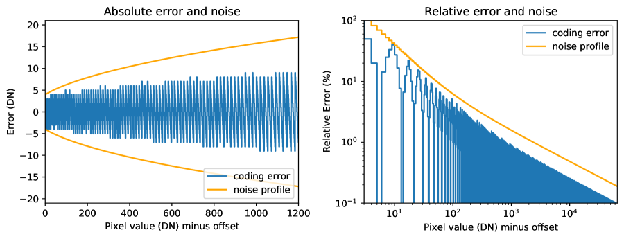
Figure 1: Square root coding is lossy and therefore induces value-specific error when decoded. Properly tuned coding schemes keep the coding error slightly below the other existing noise sources, saving bits and reducing unnecessary signal entropy. Coding 16 bits to 10 bits as shown maintains the coding error a factor of 2-3 under the calculated existing noise level, throughout the dynamic range, for a particular noise model that includes both Poisson statistics and camera dark/read noise (see text).

2 Square Root Coding

Square root coding is a simple lossy digital compression scheme that works by matching the digital transition scale to anticipated photon noise level across the dynamic range of an instrument (Gowen & Smith, 2003). Taking the direct square root of an (unsigned integer) data value reduces the number of bits by a factor of two. In a system with one quantum (e.g., photon) count per digitizer number (DN), and no detector offset, this matches the transition step size to the value-dependent variance of the quantum (“shot”) noise in each measurement. Gowen & Smith (2003) discuss the development of a modified square-root law that takes offset values into account: both digitizer gain and digitizer offset in a typical detector. PUNCH has a digitizer gain of 1 DN per 4.3 detected photons, dark/read noise that is modeled as normally distributed with $\sigma=5$ DN, and a programmable camera offset intended to operate near 100-200 counts out of a digitizer range of $2^{16}$ counts. We adopted the in-flight coding scheme

$$c=\sqrt{aP}\,,$$ (1)

where integer (rounded) arithmetic is assumed at each step (because it takes place onboard the spacecraft), $P$ is the pixel value direct from the camera or summed across multiple exposures up to 19 bits, and $c$ is the coded pixel value. The constant $a$ is programmable to generate values of $c$ with between 9-14 bits of dynamic range. In typical single-exposure operation, 16-bit camera values are square-root coded to 10-bit depth; this is accomplished by setting $a=16$. The values are then decoded on the ground to recover values approximating $P$. We began with the simple integer-arithmetic decoding scheme

$$B=(c\times c)\,/\,a\,,$$ (2)

where the division is rounded to the nearest integer.

Figure 1 shows the distribution of quantization error, vs. Poisson noise, over a typical dynamic range for the PUNCH camera. The quantization error is always well inside the Poisson noise envelope, so that quantization is dithered by 1-4 steps across the entire dynamic range, retaining smooth representation of the dynamic range, compared to the square root step size, when averaged across pixels. Information about each particular sample of the Poisson noise is lost, reducing the entropy of the remaining bits and improving the compression ratio for any subsequent compression.

3 Initial results

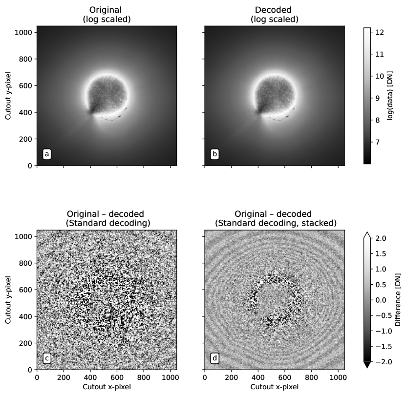
Figure 2: A visual comparison of an original dataset (a) and the encoded / decoded version (b) yields no immediately perceptible difference. However, when taking a difference map (c) and scaling to ±2 DN, a visual banding pattern appears. Beating down the noise by averaging 10 copies of the image, each with a different noise field, reduces the noise and reveals the systematic banding pattern (d).

We tested the encoding scheme in Section 2 against existing data from the STEREO/COR2 instrument (Howard et al., 2008). We summed 32 images of floating-point COR2 data from a deep-field campaign (DeForest et al., 2018b), scaled the result to PUNCH-like 16 bit values, added normally-distributed photon noise to match the PUNCH single-exposure characteristics, square-root coded the data, and then decoded them. Figure 2 shows the original data in panel (a) and a reconstituted version, coded with Equation  1 and decoded with Equation 2, in panel (b). A difference image between the original (a) and reconstituted (b) images is also displayed in panel (c), which is is scaled to a dynamic range of $\pm$2 DN. Despite the fact that the digital transitions are below the constructed noise floor of the dynamic range, square root coding produced visible artifacts in the smooth gradient of the F corona. This is a residual effect that is present under correct transition levels that are fully dithered by the Poisson noise, and is distinct from artifacts that are to be expected when the coded digital steps are comparable to (or larger than) the Poisson noise variance at a given pixel value. The peak amplitude of the artifacts can be seen in Figure 3 and is approximately $\pm$0.5 DN, much smaller than the quantization errors would be in the absence of dithering. (Quantization error on any one sample is roughly $\sqrt{P}/4$, or 10-80 DN in this dynamic range). To further illustrate the artifacts, we generated 10 copies of the source image, each with an individual sample of the noise field. We averaged all the copies together to “beat down” the noise after decoding, revealing more clearly the banding artifacts in panel (d).

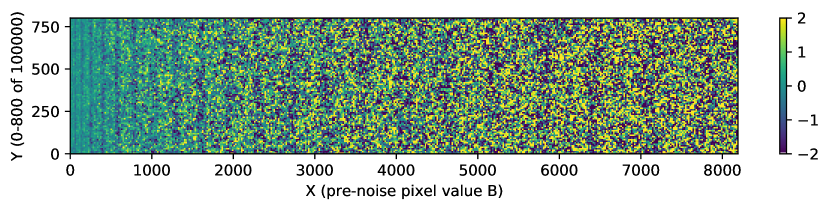
Figure 3: Difference between original and noisy, square-root coded versions of a simple gradient image shows vertical artifacts. The original image is 8192 pixels wide, and the value of each pixel is the X coordinate. The image was degraded with modeled photon noise based on the CCD model in the text, then square-root coded from 16 to 10 bits and decoded again. The figure shows the difference between the processed image and the original gradient image. Vertical stripes occur at values that the decoding systematically over- or under-estimates, revealing the source of the artifacts in Figure 2(c-d).

To understand the artifacts in Figure 2, we analyzed a simple horizontal gradient image whose value (in DN) was equal to the $x$ coordinate (in pixels), over a horizontal range of 0–8192 (0–$2^{13}$), with 100,000 samples of each input value. We added modeled Poisson and dark noise to the image, to mimic a modeled PUNCH detector; then coded and decoded the noisy gradient image as in Figure 2.

Figure 3 is a difference image between the original clean gradient and the noisy, processed version. Vertical dark artifacts in the processed image reveal a value-dependent systematic error in the square-root-processed data. Figure 4 plots the column-average difference between the original and decoded gradient images. The systematic offsets have an RMS amplitude of 0.24 DN; they are therefore strongly statistically significant toward the lower end of the gradient (left side of plot), and remain significant at the upper end of the range we considered. This is true even though the systematic offsets are small compared to the photometric noise or (smaller) square-root coding error in any one pixel; the imposed coding errors are only revealed upon deep averaging to reduce noise and determine the mean value of a large ensemble of pixels – in this case, $10^{5}$ pixels for each integer value between 0-8192.

We attribute the systematic pattern in the offsets to the fact that the square root operation is performed with both an integer domain and integer range. This means that the interval of photometric values supported by any one coded value varies slightly from the analytic ideal, yielding local nonlinear features in the square root mapping. These variations are larger than the overall nonlinearity of the analytic square root function, and have a correspondingly larger effect on the mean of an applied normal distribution of noise.

4 A Bayesian Square Root Decoder

To produce a better square root decoder than directly squaring coded values, we used a Bayesian inversion to determine better decoded values.

Each possible coded value $i$ corresponds to a range of ideal photometric input brightnesses. Taking $B_{i}$ to be the naïve decoded value corresponding to $c=i$, one may calculate the probability distribution of values for a noisy measurement $\hat{B}_{i}$ of a pixel with ideal (noise free value) $P$ that happens to be equal to $B_{i}$. In the presence of noise, the actual pixel value will be

$$\hat{P}\equiv P+N(\sigma_{i})$$ (3)

where $N(\sigma_{i})$ is a normally distributed random variable with sigma corresponding to the pixel value $B_{i}$. The normal distribution has mean zero, so that the expected value of $\hat{P}$, given the noise-free value of $P$, is just

$$\left\{\,\left<\hat{P}\right>\,|\,(P=B_{i})\,\right\}=P=B_{i}\,.$$ (4)

However, what’s available after coding/decoding is not $\hat{P}$ but $\hat{B}$. For each $B_{i}$ value (corresponding to coded value $i$), we therefore define a $P_{i}\equiv B_{i}$, apply noise to determine $\hat{P}_{i}$, and consider the noisy value $\hat{B}_{i}$ associated with each value $\hat{P}_{i}$:

$$\hat{B}_{i}\equiv D\left(C\left(\hat{P}_{i}\right)\right)\,,$$ (5)

where $C()$ represents coding and $D()$ represents decoding (in this case via Equations 1 and 2, respectively). The problem illustrated in Figure 3 is that decoding and coding are not well behaved, so that

$$\Delta B_{i}\equiv\left\{\,\left<\hat{B}_{i}\right>\,|\,(P=B_{i})\,\right\}-B_{i}\neq 0\,.$$ (6)

$\Delta B_{i}$ is the systematic offset of the expected value $\left<\hat{B}_{i}\right>$ of the decoded pixel value $\hat{B}_{i}$, given an a priori “ideal” measurement of value $B_{i}$, the coding scheme, and an a priori known noise distribution.

One may use $\Delta B_{i}$ to estimate, via the Bayesian inversion, the expected value $\left<P_{i}\right>$ of the noise-free photometric brightness, given a measured brightness value $\hat{B}_{i}$ produced by coding and then decoding a noisy photometric value. With the assumption that both the noise characteristics and $\Delta B_{i}$ vary slowly with respect to the coded-value index $i$ (as observed in Figure 3), we can immediately write a first-order approximation:

$$\left\{\,\left<P\right>\,|\,(\hat{B}=B_{i})\,\right\}\approx B_{i}-\Delta B_{i}\,,$$ (7)

where again $B_{i}$ is the naïvely decoded value corresponding to $c=i$. Equation 7 follows from Equation 6 using Bayes’ Theorem (e.g., Feller, 1968, p. 124) to reverse the roles of measured and inferred values, as detailed in an Appendix to this article.

The assumption that $\Delta B_{i}$ varies slowly with respect to $i$ (or, equivalently, $P$) is robust over small changes in $P$ between values of $i$, provided that the coded bit count is set correctly for the a priori known noise width $\sigma_{i}$. That is because $\left<\hat{P}_{i}\right>$ is an ensemble average across the entire noise distribution $N(\sigma_{i})$, centered on the interval represented by the coded value $i$. In the example case shown in Figure 1, $\sigma_{i}$ spans an interval of $\pm 4$ coded values over nearly all of the original 16-bit dynamic range; this averaging attenuates variations at the $\Delta i=1$ scale by a factor of order 10, and smaller variations (e.g., between adjacent P values) by a factor that grows as the inverse square of the scale.

With modern computers it is no challenge to assemble a complete decoding table, explicitly calculating $\Delta B_{i}$ for every possible value of $i$, for a complete code table as many as 20 bits deep. We carried out the calculation explicitly for each possible coded pixel value for a 10-bit-deep square root coding scheme operating on 16 bit data, using the modeled noise levels and camera performance used in Figure 3. These camera effects include modeled dark-current and digitizer offset values, to simulate the actual noise performance of a typical CCD camera; but these features of the noise model are negligible compared to Poisson noise over most of the coded dynamic range. For each $i$ we calculated $B_{i}$ and enumerated the probability distribution for $\hat{P}_{i}$ across $\pm 4\sigma$ of the modeled Poisson-plus-dark noise for the PUNCH detectors, sampling the distribution at 10,000 individual points. We then coded and decoded each of the 10,000 resulting $\hat{P}_{i}$ values and explicitly evaluated $\left<\hat{P}_{i}\right>$ to determine $\Delta B_{i}$ for each value of $i$ and thereby construct a first-order corrected decoding table.

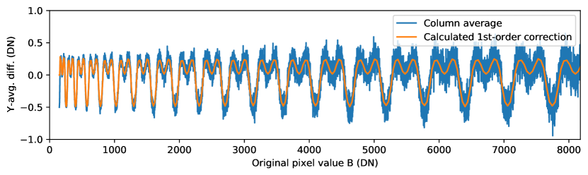
Figure 4: Column-averaged value of all 100,000 rows of the image in Figure 3 reveals systematic error from naïve square root coding of each possible pixel value, in the presence of noise. First-order correction via Equation 7 visually matches the offsets.

We used lookup into the corrected decoding table as a first-order Bayesian square-root decoder. Applying that Bayesian decoder to the same data as used in Figure 3 reduced the systematic offsets by approximately a factor of four, as shown in Figure 5; residual systematic fluctuations in the column averages in Figure 5 are below, but comparable to, the reduced noise floor after averaging.

The blue difference curve in Figure 5 retains obvious low-frequency residuals that follow the slope of the first-order correction. Fortunately, second-order correction is also available. Equation 7 relies on the constancy of the slope $d(\Delta B_{i})/d(P_{i})$; including the second-order term of the Taylor expansion (based on observing Figure 5) yields

$$\left\{\,\left<\hat{P}_{i}\right>\,|\,(c=c_{i})\,\right\}\approx B_{i}-\Delta B_{i}-\frac{1}{2}\frac{d\Delta B_{i}}{di}\,,$$ (8)

where the derivative nomenclature is used to emphasize that $\Delta B_{i}$ and its rate of change are assumed to vary slowly compared to the (integer) steps in $i$. The orange curve in Figure 5 shows this second-order term, calculated from the discrete numeric derivative of the $\Delta B_{i}$ curve in Figure 3.

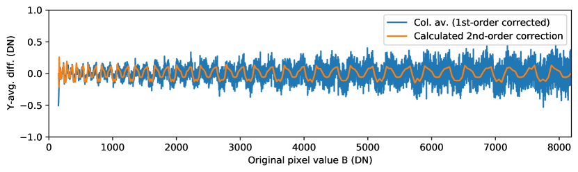
Figure 5: Column-averaged values of the image in Figure 3, with the first-order correction applied, reveal greatly reduced systematic error. A second-order correction, allowing for the rate of change of $\Delta B_{i}$ with respect to $i$, visually matches the residuals from first-order correction.

We used Equation 8 to assemble a second-order correction table and square root decoder. Figure 6 shows the result of second-order decoding. The overlain curves show the 49-value running mean of the offset, further beating down the noise intrinsic to the image and revealing the systematic variation. We found the RMS value of the uncorrected systematic curve, between CCD pixel values of 500 and 4000, to be 0.23 DN. The RMS value of the second-order corrected systematic curve over the same range is 0.012 DN, corresponding to a $20\times$ improvement in systematics; this enables meaningful averaging of up to roughly $10^{6}$-$10^{7}$ CCD readout values over this portion of the dynamic range, provided that other systematics are eliminated to the same degree of precision.

To test how robust the Bayesian offset estimation might be against errors in the noise model itself, we regenerated the analysis of Figures 4-6, using noise models a factor of two higher or lower than the actual simulated CCD noise level, to identify how sensitive the correction might be to exact determination of the noise level in the original measurements. Shrinking or expanding the variance of the table noise model by a factor of two yielded RMS residuals of 0.014 DN and 0.013 DN respectively over the 500-4000 DN domain. We conclude that the inversion method is robust against factor-of-two discrepancies between the specific noise model used to calculate the correction table, and the corresponding noise characteristics of the original measurement, provided that the dithering condition holds for both the actual and modeled noise level.

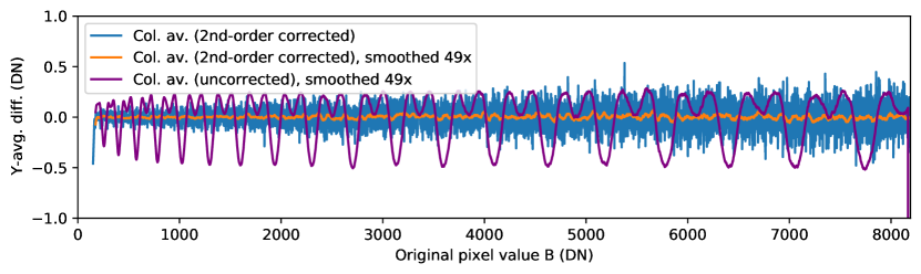
Figure 6: Column-averaged values of the image in Figure 3, with the second-order correction applied, reveal still further reduced systematic error. The blue curve is a direct column average across all 100,000 samples per value; the orange curve is further averaged across 49 pixel values, beating down noise still further to reveal the systematic offsets. The uncorrected systematic error is also plotted, for comparison. The 2nd order corrected systematic decoding error is reduced roughly $20\times$ compared to the systematic decoding error from the naïve decoding scheme.

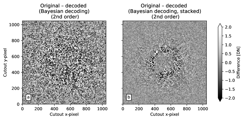
Figure 7: Copy of Figure 2 panels (c) and (d), using the second-order Bayesian decoder instead of direct square-root decoding, eliminates the visual artifacts seen with direct analytic square-root decoding..

To return to the initial dataset, Figure 7 provides a comparison similar to Figure 2, but using the second order Bayesian decoder. In both the difference map in panel (a) and the stacked version in panel (b), the visible banding artifacts have been visually eliminated.

5 Discussion & Conclusions

We have demonstrated an improved method for square-root decoding that greatly reduces systematic coding error compared to direct methods. The algorithm is implemented in a Jupyter notebook that has been released via Zenodo (DeForest et al., 2022).

The improved Bayesian square root decoder we describe is immediately applicable to the PUNCH mission, which requires averaging over many individual pixels in space and time to achieve the photometric precision required by that mission; but it is also applicable to other instruments and other post-processing schemes that require high photometric precision relative to the photometric noise in a single measurement. Square root coding is a common technique in data-volume-constrained applications with photon-limited imaging; Bayesian analysis is important for this and other coding schemes, to ensure that photometry is fully preserved in the resultant reconstituted images.

The method we described uses only post-facto analysis to produce a new decoding table without reference to the actual data being produced, and only moderate (factor-of-two) agreement is required between the actual noise characteristics of the instrument and the noise model used to assemble the table. Consequently, the method is applicable not only to new instruments but also to existing missions or observatories and even to archival data from instruments that no longer exist, provided that the coding scheme is known. Further, because the method uses direct numerical inversion, rather than analytic calculation, to determine corrected decoding values, it is applicable to other nonlinear coding schemes than the scaled square root, provided only that the $\Delta B_{i}$ from noise-affected ensembles of measurements varies slowly with respect to the ideal noise-free pixel value P or, equivalently, the coded-value index $i$. In this respect, our method is more general, though potentially less precise under ideal conditions, than direct analytic treatments (e.g., Bernstein et al., 2010) optimized to a particular observing scenario and coding scheme.

In our particular case, the important nonlinearity did not arise from the square root operator itself, but rather from the interaction between the integers and the locations, in the decoded representation, of digital transitions in the coded values. In other cases, such as the polarimetric measurements explored by Inhester et al. (2021), a mathematical transformation itself, even without integer transitions, may produce counter-intuitive behavior in the presence of normally distributed noise. In both our case and the study by Inhester et al., the most important effect is that a zero-mean noise distribution can produce nonzero-mean distributions in transformed data products. Other higher-order effects on probability distributions exist, and could in principle cause confusion between, for example, significant and insignificant features in a noisy data set.

More generally, careful thought is necessary, in order to preserve the greatest possible utility of the data, when making compromises in representation or compression. While first-order effects (such as direct digital transition errors) are easy to mitigate (for example through dithering), careful thought in advance of implementation can also mitigate or remove second order effects (such as the coding error we identified here), greatly enhancing the data’s utility.

Even more broadly, nonlinear systems interact with noise in counter-intuitive ways. Bayesian analysis is a valuable tool to understand the interaction between nonlinear analysis steps and noise properties of any data product (including reconstituted “raw” data), even if the noise sources in the original data are well-behaved.

6 Appendix

In stepping from Equation 6 to Equation 7 we breezily invoked Bayes’ Theorem. Here we demonstrate through analysis how that step follows from the theorem. The inference is ultimately tested, and even refined, in the main text through numerical treatment rather than direct analysis (e.g., Figures 5 and 6); but it is a useful exercise to trace the logic back to the general theorem.

Bayes’ Theorem converts between conditional probabilities. It is just

$$\mathbb{P}(A|B)=\mathbb{P}(B|A)\frac{\mathbb{P}(A)}{\mathbb{P}(B)}\,,$$ (9)

where $\mathbb{P}$ represents probability of an outcome. In this case, the two variables of interest are the true (noise-free) pixel value $P$ and the coded/decoded, noisy pixel value ${\hat{B}}$. $P$ has a uniform prior distribution; and in the absence of information about $P$, so does $\hat{B}$ (neglecting edge effects at the top and bottom of the dynamic range and the very small effect of noise level variation across the width of the noise distribution itself), although the two quantities are related by the normal random variable $N$. Therefore, to very good approximation,

$$\mathbb{P}\left(P=j|{\hat{B}}=B_{i}\right)=\ N_{i}^{-1}\,\mathbb{P}\left({\hat{B}}=B_{i}|P=j\right)\,,$$ (10)

where $N_{i}$ is the number of discrete values of $j$ that convert to the coded value $i$. Multiplying each term of Equation 10 by $j$ and summing over all values of $j$ yields:

$$\left\{\left<P\right>|({\hat{B}}=B_{i})\right\}=\ \sum_{j}\left\{\frac{j}{N_{i}}\mathbb{N}\left((j-B_{i})/\sigma(B_{i})\right)\right\}\approx\sum_{k}\left\{B_{k}\frac{N_{k}}{N_{i}}\mathbb{N}((B_{k}-B_{i})/\sigma(B_{i}))\right\}\,,$$ (11)

where $k$ runs over the same values as $i$, and $N_{k}$ is the number of discrete values of $j$ that convert to the coded value $k$. The second step involves grouping all values of $j$ that lead to a single coded value $k$. The approximation arises from ignoring variation of $\mathbb{N}$ across those values, which is equivalent to treating $\mathbb{N}$ as piecewise linear across each coded interval. That egregious sin sidesteps integrating the Gaussian for this approximate analysis. Extracting $B_{i}$ from the sum gives

$$\left\{\left<P\right>|({\hat{B}}=B_{i})\right\}\approx B_{i}-\sum_{k}\left\{B_{k}(\frac{N_{i}-N_{k}}{N_{i}})\mathbb{N}((B_{k}-B_{i})/\sigma(B_{i}))\right\}\,,$$ (12)

which matches the form of Equation 7. In particular, the summation term in Equation 12 is the $\Delta B_{i}$ described in Equation 6; and the $(N_{i}-N_{k})$ coefficient inside the sum embodies the discrete-step perturbation described in the main text.

Contrariwise, choosing $j=B_{k}$ for some $k$, multiplying by $N_{k}B_{i}$, and summing over all values of $i$ yields:

$$\left\{\left<{\hat{B}}\right>|P=B_{k}\right\}\approx\sum_{i}\left\{\frac{N_{k}}{N_{i}}B_{i}\mathbb{N}\left((B_{i}-B_{k})/\sigma(B_{k})\right)\right\}\,,$$ (13)

where the equation is only approximate because the same linearization of $\mathbb{N}$ is used as in Equation 11. Extracting $B_{k}$ from the sum as above, and then swapping the labels of the $i$ and $k$ indices, yields

$$\left\{\left<{\hat{B}}\right>|P=B_{i}\right\}\approx B_{i}+\sum_{k}\left\{B_{k}(\frac{N_{i}-N_{k}}{N_{i}})\mathbb{N}\left((B_{k}-B_{i})/\sigma(B_{i})\right)\right\}\,,$$ (14)

which matches the form of Equation 6. The difference between Equation 12 and 14 arises because the sums are being carried out over different quantities: Equation 12 is summed over $j$ while Equation 14 is summed (with weighting) over $i$, although both arise from Equation 10. The step from Equation 6 to 7 thus follows analytically from Bayes’ Theorem and the approximation given; this supports the intuition that, to linear order, small-offset perturbations can be inverted by merely reversing the direction of the perturbation. The piecewise-linear approximation used here is somewhat aggressive, and highlights the importance of higher order correction (described and carried out numerically in the main text).

References

- Acton et al. (1992) Acton, L., Tsuneta, S., Ogawara, Y., et al. 1992, Science, 258, 618, doi: 10.1126/science.258.5082.618
- Bernstein et al. (2010) Bernstein, G. M., Bebek, C., Rhodes, J., et al. 2010, PASP, 122, 336, doi: 10.1086/651281
- de Boer (1996) de Boer, C. R. 1996, A&AS, 120, 195
- DeForest (2017) DeForest, C. E. 2017, ApJ, 838, 155, doi: 10.3847/1538-4357/aa67f1
- DeForest et al. (2018a) DeForest, C. E., Gibson, S. E., Killough, R. L., & Henry, A. 2018a, in AGU Fall Meeting Abstracts, Vol. 2018, SH43B–3703
- DeForest et al. (2018b) DeForest, C. E., Howard, R. A., Velli, M., Viall, N., & Vourlidas, A. 2018b, ApJ, 862, 18, doi: 10.3847/1538-4357/aac8e3
- DeForest et al. (2022) DeForest, C. E., Lowder, C., Seaton, D. B., & West, M. J. 2022, Bayesian analysis of square-rooted values, Zenodo, doi: 10.5281/zenodo.6672640
- Feller (1968) Feller, W. 1968, An Introduction to Probability Theory and Its Applications, Vol. 1 (Wiley). http://www.amazon.ca/exec/obidos/redirect?tag=citeulike04-20{&}path=ASIN/0471257087
- Feller (1971) Feller, W. 1971, An introduction to probability theory and its applications, Vol. 1 (John Wiley & Sons), pp. 190ff
- Golub et al. (2007) Golub, L., Deluca, E., Austin, G., et al. 2007, Sol. Phys., 243, 63, doi: 10.1007/s11207-007-0182-1
- Goodrich et al. (2004) Goodrich, J. N., Kholikov, S., Lindsey, C., et al. 2004, in Society of Photo-Optical Instrumentation Engineers (SPIE) Conference Series, Vol. 5493, Optimizing Scientific Return for Astronomy through Information Technologies, ed. P. J. Quinn & A. Bridger, 538–546, doi: 10.1117/12.552085
- Gowen & Smith (2003) Gowen, R. A., & Smith, A. 2003, Review of Scientific Instruments, 74, 3853, doi: 10.1063/1.1593811
- Howard et al. (2008) Howard, R. A., Moses, J. D., Vourlidas, A., et al. 2008, Space Sci. Rev., 136, 67, doi: 10.1007/s11214-008-9341-4
- Inhester et al. (2021) Inhester, B., Mierla, M., Shestov, S., & Zhukov, A. N. 2021, Sol. Phys., 296, 72, doi: 10.1007/s11207-021-01815-3
- Nieto-Santisteban et al. (1999) Nieto-Santisteban, M. A., Fixsen, D. J., Offenberg, J. D., Hanisch, R. J., & Stockman, H. S. P. 1999, in Astronomical Society of the Pacific Conference Series, Vol. 172, Astronomical Data Analysis Software and Systems VIII, ed. D. M. Mehringer, R. L. Plante, & D. A. Roberts, 137
- Park et al. (2020) Park, E., Moon, Y.-J., Lim, D., & Lee, H. 2020, ApJ, 891, L4, doi: 10.3847/2041-8213/ab74d2
- Scherrer et al. (1995) Scherrer, P. H., Bogart, R. S., Bush, R. I., et al. 1995, Sol. Phys., 162, 129, doi: 10.1007/BF00733429
- Seaton et al. (2013) Seaton, D. B., Berghmans, D., Nicula, B., et al. 2013, Sol. Phys., 286, 43, doi: 10.1007/s11207-012-0114-6
- Yaroslavsky (1996) Yaroslavsky, L. P. 1996, in Society of Photo-Optical Instrumentation Engineers (SPIE) Conference Series, Vol. 2825, Wavelet Applications in Signal and Image Processing IV, ed. M. A. Unser, A. Aldroubi, & A. F. Laine, 2–13, doi: 10.1117/12.255218