Statistics of the interaural parameters for dichotic tones in diotic noise ($\textup{N}_{0}\textup{S}_{\psi}$)

Abstract

Stimuli consisting of an interaurally phase-shifted tone in diotic noise - often referred to as $\textup{N}_{0}\textup{S}_{\psi}$ - are commonly used in the field of binaural hearing. As a consequence of mixing diotic noise with a dichotic tone, this type of stimulus contains random fluctuations in both interaural phase- and level-difference. This study reports the joint probability density functions of the two interaural differences as a function of amplitude and interaural phase of the tone. Furthermore, a second joint probability density function for interaural phase differences and the instantaneous power of the stimulus is derived.

1 Introduction

Tone in noise detection thresholds improve when the interaural configuration of tone and noise differ compared to the diotic case. A rich literature reports on the influence of virtually every parameter of acoustic stimuli on this binaural unmasking [see e.g. 1, for a review]. Amongst these parameters the phase difference $\psi$ introduced between the target tones of the two ear-signals is fundamental and was explored already in the first study of dichotic tone in noise detection by Hirsh1948 [2]. Such a signal is commonly referred to as $\textup{N}_{0}\textup{S}_{\psi}$ where the subscripts indicate the interaural phase difference (IPD) of the noise (N) or signal (S). The difference between the detection threshold for the purely diotic $\textup{N}_{0}\textup{S}_{0}$ and the $\textup{N}_{0}\textup{S}_{\psi}$ signal is referred to as the binaural masking level difference (BMLD) and is largest for the case where $\psi=\pi$ [2].

Adding a dichotic $S_{\psi}$ tone to diotic $N_{0}$ noise introduces an incoherence between the left and right signals – which in turn results in random fluctuations of the interaural phase and level differences (IPD, ILD) (visualized in Fig. 1(a)). The incoherence increases with the tone level so that binaural unmasking and incoherence detection are often treated synonymously [3]. The value of interaural coherence itself however was found to be an insufficient predictor for incoherence detection performance. Instead, detection performance correlated with the amount of IPD and ILD fluctuations as measured by the standard deviation [4]. Knowledge about the statistical processes that underlay these fluctuations can thus be instrumental for binaural modeling as well as stimulus design. Only relatively few studies, however, have previously treated these statistics. The probability density function (PDF) underlying the statistical distribution of IPDs in incoherent noise has been derived in the frame of optical interferometry [5]. Henning1973 [6] derived the PDF for IPDs in the special case of $\textup{N}_{0}\textup{S}_{\pi}$ and using a very similar approach for the same stimulus condition, Zurek1991 [7] additionally derived marginal PDFs for ILDs. Other studies seemed to also have worked on stimuli where the tone IPD did not equal $\pi$ but his work seemed to have remained unpublished [8]. This study closes this gap by deriving a closed form expression for the joint PDF of IPDs and ILDs in the general case of a $N_{0}S_{\psi}$ stimulus. From this distribution, the marginal PDFs can also be calculated by means of numerical integration.

If fluctuations of the IPD are indeed a cue used to detect the tone in an $\textup{N}_{0}\textup{S}_{\psi}$ stimulus, then the stimulus energy at which these fluctuation occurred might also affect performance. The product of the left and right ear stimulus envelope, here called $P^{\prime}$, can be interpreted as a measure of instantaneous stimulus power. Consequently, this study also drives the joint PDF for $P^{\prime}$ and IPD.

2 Deriving the probability density functions

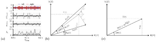
Figure 1: (a) Visualization of the random fluctuations in IPD $\Delta\Phi(t)$ and ILD $\Delta L(t)$ and $P^{\prime}$ due to mixing an antiphasic 500Hz tone with a $500\text{\,}\mathrm{Hz}$ wide band of diotic noise (SNR=$-10\text{\,}\mathrm{dB}$). (b) Complex-plane representation of the components in a $\textup{N}_{0}\textup{S}_{\psi}$ stimulus. The left-ear-signal is constructed by adding a “tone”-vector with length $C$ and angle $+\nicefrac{{\psi}}{{2}}$ to the noise vector $X(t)+iY(t)$. The right-ear-signal is constructed by adding a “tone”-vector with an angle of $-\nicefrac{{\psi}}{{2}}$ to the same noise. (c) Complex-plane representation of the interaural-baseband $Z(t)=\Xi(t)+i\Upsilon(t)$ which is gained by dividing the left-ears-baseband by the right-ears-baseband. The absolute value of the baseband equals the interaural amplitude ratio $R$ while the phase equals the interaural phase difference $\Delta\Phi$.

If $N$ is a Gaussian bandpass noise process with a mean value of zero, the process can be represented using its in-phase and quadrature components $X$ and $Y$:

$$N(t)=X(t)\cos(\omega_{0}t)-Y(t)sin(\omega_{0}t),$$ (1)

where $X$ and $Y$ are orthogonal noise processes with the same variance and mean as $N$. The reference frequency $\omega_{0}$ is conveniently chosen to equal the frequency of the tone $S(t)=C\cos(\omega_{0}t+\psi)$ which is added with the amplitude $C$ and phase $\psi$. The resulting stimulus can then be expressed as:

$$W(t)= \left[X(t)+C\cos(\psi)\right]\cos(\omega_{0}t)$$

$$-[Y(t)+C\sin(\psi)]\sin(\omega_{0}t).$$ (2)

Or alternatively, employing the signals complex baseband $Z(t)$:

$$W(t) =\Re\left\{Z(t)\textup{e}^{i\omega_{0}t}\right\}$$ (3)

$$Z(t) =\left[X(t)+C\cos(\psi)\right]+i\left[Y(t)+C\sin(\psi)\right]$$

$$=A(t)\textup{e}^{i\Phi(t)}$$ (4)

where $\Re(x)$ extracts the real part, $i=\sqrt{-1}$ is the imaginary unit and $A(t)$, $\Phi(t)$ are the instantaneous amplitude and phase of the baseband.

In case of the $\textup{N}_{0}\textup{S}_{\psi}$ stimulus, a cosine with phase $\nicefrac{{\psi}}{{2}}$ is added to the noise in the left-ear signal while the phase of the cosine in the right-ear signal is $\nicefrac{{-\psi}}{{2}}$. This process is shown in Fig. 1(b) where the individual components are visualized as vectors in the complex plane. Applying Eq. (4) results in the complex basebands for the left- and right-ear signals $Z_{L}(t)$ and $Z_{R}(t)$.

Based on these expressions, PDFs for the interaural parameters will be derived using two separate approaches. In the first approach, the baseband of the left-ear signal $Z_{L}(t)$ is divided by the baseband of the right-ear signal $Z_{R}(t)$ resulting in the interaural baseband $Z_{1}(t)$:

$$Z_{1}(t) =\frac{Z_{R}(t)}{Z_{L}(t)}=\frac{A_{R}(t)}{A_{L}(t)}\textup{e}^{i[\Phi_{R}(t)-\Phi_{L}(t)]}$$

$$=R(t)\textup{e}^{i\Delta\Phi(t)},$$ (5)

where $\Delta\Phi(t)$ and $R(t)$ are the instantaneous IPDs and the interaural amplitudes ratios (IARs) respectively. Instantaneous ILDs can then be calculated as: $\Delta L(t)=20\log_{10}R(t)$. To derive the PDF for IPDs and the product of the left and right-ear envelope $P^{\prime}$, $Z_{L}(t)$ is multiplied with the complex conjugate of $Z_{R}(t)$ resulting in

$$Z_{2}(t) =Z_{R}(t)Z^{*}_{L}(t)=A_{R}(t)A_{L}(t)\textup{e}^{i[\Phi_{R}(t)-\Phi_{L}(t)]}$$

$$=P^{\prime}(t)\textup{e}^{i\Delta\Phi(t)},$$ (6)

The process of deriving the PDFs from Eq. (5) and Eq. (6) follows the exact same rational so that the process will only be detailed for Eq. (5) the results for the second approach will then be stated without further detail.

For the interaural baseband, $Z_{L}$ and $Z_{R}$ as resulting form Eq. (2) are inserted into Eq. (5) resulting in:

$$Z_{1}(t) =\Xi(t)+i\Upsilon(t)$$

$$=\frac{C\cos{\left(\nicefrac{{\psi}}{{2}}\right)}+i\left[C\sin{\left(\nicefrac{{\psi}}{{2}}\right)}+Y{\left(t\right)}\right]+X{\left(t\right)}}{C\cos{\left(\nicefrac{{\psi}}{{2}}\right)}-i\left[C\sin{\left(\nicefrac{{\psi}}{{2}}\right)}-Y{\left(t\right)}\right]+X{\left(t\right)}}$$ (7)

$$\Xi(t) =\frac{Y^{2}{\left(t\right)}+\left[C\cos{\left(\nicefrac{{\psi}}{{2}}\right)}+X{\left(t\right)}\right]^{2}-C^{2}\sin^{2}{\left(\nicefrac{{\psi}}{{2}}\right)}}{\left[C\sin{\left(\nicefrac{{\psi}}{{2}}\right)}-Y{\left(t\right)}\right]^{2}+\left[C\cos{\left(\nicefrac{{\psi}}{{2}}\right)}+X{\left(t\right)}\right]^{2}}$$ (8)

$$\Upsilon(t) =\frac{2C\left[C\cos{\left(\nicefrac{{\psi}}{{2}}\right)}+X{\left(t\right)}\right]\sin{\left(\nicefrac{{\psi}}{{2}}\right)}}{\left[C\sin{\left(\nicefrac{{\psi}}{{2}}\right)}-Y{\left(t\right)}\right]^{2}+\left[C\cos{\left(\nicefrac{{\psi}}{{2}}\right)}+X{\left(t\right)}\right]^{2}},$$ (9)

where $\Xi(t)$ and $\Upsilon(t)$ are the in-phase and quadrature components. As visualized in Fig. 1(b), the instantaneous IPDs and IARs can be calculated as $\Delta\Phi(t)=\operatorname{arctan2}\left(\Upsilon(t),~{}\Xi(t)\right)$ and $R(t)=\sqrt{\Upsilon(t)^{2}+\Xi(t)^{2}}$. Here, $\operatorname{arctan2}$ is the two-argument arctangent which returns the angle in the euclidean plane.

Both Random Processes $R$ and $\Delta\Phi$ are functions of $X$ and $Y$ which are uncorrelated Gaussian noise processes with the variance $\sigma^{2}$. The joint PDF $f_{X,Y}(x,y)$ of $X$ and $Y$ is thus that of a bivariate Gaussian distribution:

$$f_{X,Y}(x,y)=\frac{1}{2\pi\sigma^{2}}\textup{e}^{-\frac{1}{2\sigma^{2}}\left(x^{2}+y^{2}\right)},$$

$$1=\iint\limits^{\infty}_{-\infty}\frac{1}{2\pi\sigma^{2}}\textup{e}^{-\frac{1}{2\sigma^{2}}\left(x^{2}+y^{2}\right)}\textup{d}x\,\textup{d}y,$$ (10)

to derive Eq. (10) as a function of $\xi$ and $\upsilon$ which are instances of the processes $\Xi$ and $\Upsilon$, Eqs. (8) and (9) are rearranged to gain $x$ and $y$ as functions of $\xi$ and $\upsilon$:

$$x(\xi,\upsilon) =C\left[\frac{2\upsilon\sin{\left(\nicefrac{{\psi}}{{2}}\right)}}{\upsilon^{2}+\left(\xi-1\right)^{2}}-\cos{\left(\nicefrac{{\psi}}{{2}}\right)}\right],$$

$$y(\xi,\upsilon) =\frac{C\left(\upsilon^{2}+\xi^{2}-1\right)\sin{\left(\nicefrac{{\psi}}{{2}}\right)}}{\upsilon^{2}+\xi^{2}-2\xi+1}$$ (11)

Furthermore, by using the Jacobian determinant $\left|J(x,y)\right|$:

$$\textup{d}x\,\textup{d}y=\left|J(x,y)\right|\textup{d}\xi\,\textup{d}\upsilon=\frac{4C^{2}\sin^{2}{\left(\nicefrac{{\psi}}{{2}}\right)}}{\left[\upsilon^{2}+\left(\xi-1\right)^{2}\right]^{2}}\textup{d}\xi\,\textup{d}\upsilon.$$ (12)

Applying the transformations in Eqs. (11) and (12) to change the variables of Eq. (10) results in:

$$1 =\frac{2C^{2}\sin^{2}\left(\nicefrac{{\psi}}{{2}}\right)}{\pi\sigma^{2}}$$

$$\times\iint\limits^{\infty}_{-\infty}\frac{\textup{e}^{-\frac{C^{2}\left[\upsilon^{2}-2\upsilon\sin{\left(\psi\right)}+\xi^{2}-2\xi\cos{\left(\psi\right)}+1\right]}{2\sigma^{2}\left[\upsilon^{2}+\left(\xi-1\right)^{2}\right]}}}{\left[\upsilon^{2}+\left(\xi-1\right)^{2}\right]^{2}}\textup{d}\xi\,\textup{d}\upsilon.$$ (13)

To derive the joint PDF $f_{R,\Delta\Phi}(r,\Delta\varphi)$ which generates the IARs $r$ and IPDs $\Delta\varphi$. Eq. (13) is transformed from rectangular to polar coordinates by using the transforms: $\xi=r\cos{\Delta\varphi}$, $\upsilon=r\sin{\Delta\varphi}$, $\textup{d}\xi\,\textup{d}\upsilon=r\,\textup{d}r\,\textup{d}\Delta\varphi$ resulting in:

$$f_{R,\Delta\Phi}(r,\Delta\varphi)=\frac{C^{2}2r\sin^{2}\left(\nicefrac{{\psi}}{{2}}\right)}{\sigma^{2}\pi h(0)^{2}}\textup{e}^{-\frac{C^{2}h(\psi)}{\sigma^{2}2h(0)}}$$ (14)

where $h(\psi)=r^{2}-2r\cos(\Delta\varphi-\psi)+1$ and $r\in[0,\infty],~{}\Delta\varphi\in[-\pi,\pi]$

This equation can be interpreted as the distribution of all possible values of the interaural baseband $z_{1}=r\textup{e}^{i\Delta\varphi}$ and thus the distribution of all possible combinations of IPDs $\Delta\varphi$ and IARs $r$. It is also apparent from Eq. (14) that equal ratios of $\nicefrac{{C^{2}}}{{\sigma^{2}}}$ result in the same PDF so that PDFs will be referenced using the signal to noise ratio $SNR=\nicefrac{{C^{2}}}{{2\sigma^{2}}}$ instead of $\sigma^{2}$ and $C$. Some examples of these functions are shown in Fig. 2(a-c). Deriving the joint PDF of $\Delta\varphi$ and ILD $\Delta l$ instead of IAR $r$ is easily done by using transforms $a=10^{\nicefrac{{\Delta l}}{{20}}}$ and $dr=\nicefrac{{a}}{{20}}\ln(10)d\Delta l$.

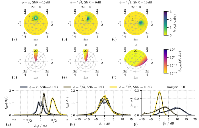
Figure 2: (a-c) Some examples of the joint PDF $f_{R,\Delta\Phi}$ given in Eq. (14). Angles in the polar plot are the IPDs $\Delta\varphi$ while the radial variable is $r$, brightness/colors indicate the probability density. (d-f) Joint PDF $f_{P^{\prime},\Delta\Phi}$ for the same parameters as in (a-c). As in the first row of plots, angles indicate the IPD $\Delta\varphi$ and brightness/colors the probability density. The radial variable however is $P^{\prime}$. PDF were calculated for a noise variance of $\sigma^{2}=1$. A logarithmically-scaled colormap was used due to the large dynamic range of the PDF. White areas indicate undefined combinations of $P^{\prime}$ and $\Delta\varphi$ (d, e) Marginal PDF for $\Delta\Phi$ and $\Delta L$ and $P^{\prime}$ compared to PDF that were estimated from the matching signal waveform.

To derive the joint PDF of $\Delta\Phi$ and $P^{\prime}$ The process detailed above is repeated based on the interaural baseband $Z_{2}$ as defined in Eq. (6) resulting in the PDF:

$$f_{P^{\prime},\Delta\Phi}(p^{\prime},\Delta\varphi) =\frac{e^{-\frac{C^{2}}{2\sigma^{2}}-\frac{p^{\prime}\left[\cos(\Delta\varphi)-\cos(\Delta\varphi-\psi)\right]}{2\sigma^{2}\left[\cos(\psi)-1\right]}}p^{\prime}}{2\pi\sigma^{2}\sqrt{g}}$$ (15)

where $g$ is given by:

$$g= 2C^{2}\sin^{2}{\left(\nicefrac{{\psi}}{{2}}\right)}\left[2p^{\prime}\cos{\left(\Delta\varphi\right)}-C^{2}\left(\cos{\left(\psi\right)}-1\right)\right]$$

$$-p^{\prime 2}\sin^{2}{\left(\Delta\varphi\right)}.$$ (16)

and the range of values is defined by:

$$p^{\prime} \in[0,\hat{p^{\prime}}(\Delta\varphi)],~{}\Delta\varphi\in[-\hat{\Delta\varphi}(p^{\prime}),+\hat{\Delta\varphi}(p^{\prime})]$$ (17)

where

$$\hat{p^{\prime}}(\Delta\varphi) =C^{2}\frac{\cos(\psi)-1}{\cos{(\Delta\varphi)}-1}.$$ (18)

The function $\hat{\Delta\varphi}(p^{\prime})$ can be gained by solving Eq. (18) for $\Delta\varphi$.

Similar to Eq. (14) which defined the distribution of all possible values of $\Delta\varphi$ and $r$, this function can be interpreted as the distribution of all possible combinations of $\Delta\varphi$ and $p^{\prime}$. The range of these combinations, however, is limited by Eq. (18) so that large areas of the exemplary PDFs shown Fig. 2(d–f) are undefined. This limitation will be treated further in the discussion.

The marginal PDFs of the IAR $R$, the IPD $\Delta\Phi$ and the product of the left and right stimulus envelope $P^{\prime}$ can be calculated from the two joint PDFs defined in Eq. (14) and Eq. (15) by integrating over the other variable.

$$f_{\Delta\Phi}(\Delta\varphi) =\int_{0}^{\infty}f_{R,\Delta\Phi}(r,\Delta\varphi)\textup{d}r$$

$$=\int_{0}^{\hat{p^{\prime}}(\Delta\varphi)}f_{P^{\prime},\Delta\Phi}(p^{\prime},\Delta\varphi)\textup{d}p^{\prime}$$ (19)

$$f_{R}(r) =\int_{-\pi}^{\pi}f_{R,\Delta\Phi}(r,\Delta\varphi)\textup{d}\Delta\varphi$$ (20)

$$f_{P^{\prime}}(p^{\prime}) =\int_{-\hat{\Delta\varphi}(p^{\prime})}^{\hat{\Delta\varphi}(p^{\prime})}f_{P^{\prime},\Delta\Phi}(p^{\prime},\Delta\varphi)\textup{d}\Delta\varphi$$ (21)

The marginal PDF for ILDs can be derived by using the transform $r=10^{\nicefrac{{\Delta l}}{{20}}}$:

$$f_{\Delta L}(\Delta l) =\frac{10^{\nicefrac{{\Delta l}}{{20}}}\log(10)}{20}\int_{-\pi}^{\pi}f_{R,\Delta\Phi}(10^{\nicefrac{{\Delta l}}{{20}}},\Delta\varphi)\textup{d}\Delta\varphi$$ (22)

As previously discussed, the PDFs of $\Delta\varphi$ as well as $\Delta l$ (and thus $r$) only depend on the SNR and not on the absolute stimulus power. $P^{\prime}$ however, is the product of the left and right stimulus envelope and must thus also depend on stimulus power. For this reason, PDFs for $P^{\prime}$ will always be shown normalized by $C^{2}$ so that PDFs only depend on the SNR and are independent of overall stimulus power.

No closed-form solution for Eq. (19)–(22) could be found so that numeric integration was used to evaluate them (QUADPACK algorithms QAGS/QAGI [9]). Figs. 2(g)–(i) show some examples of the PDF of $\Delta\Phi$, $\Delta L$, $P^{\prime}$ and verifies the results by comparing Eq.(19)–(20) to PDFs that were numerically estimated from signal waveforms.

3 Discussion

All PDFs derived above show discontinuities for $\Delta\varphi\in\{0,\pm\pi\}$ for which the probability densities approach zero. Or in other words, a $\textup{N}_{0}\textup{S}_{\psi}$ stimulus will never contain IPDs that are exactly zero or $\pi$. Both discontinuities can be understood when keeping in mind that the IPD is defined by $\Delta\varphi=\operatorname{arctan2}\left(\upsilon,~{}\xi\right)$. Which can only result in a value of $0$ or $\pm\pi$ if $\upsilon=0$. This is only the case when $x=-C\cos\left(\nicefrac{{\psi}}{{2}}\right)$. As the probability of $x$ to take this exact value approaches zero, the joint PDFs will also approach zero. For further discussion of the PDFs however, this discontinuity will not be shown explicitly in plots as it’s implication in practice is limited.

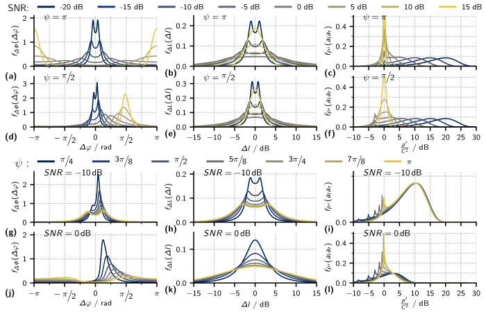
Figure 3: Exemplary marginal PDFs (a)–(f) Calculated for two fixed signal phases $\psi$ at different SNRs (color/brightness-coded) and (g)–(l) calculated at two fixed SNR for different signal phases (color/brightness coded).

Figure 3(a) and (d) show examples of the marginal IPD PDFs for $\psi=\pi$ and $\psi=\nicefrac{{\pi}}{{2}}$ while varying the SNR. The instantaneous IPD $\Delta\varphi$ can be interpreted as a result of the mixture of zero IPD due to the diotic noise and the IPD $\psi$ of the tone. The weighting of the two IPDs is determined by the instantaneous power of the noise relative to the power of the tone. Thus, at large negative SNRs where the stimulus is dominated by noise, IPD PDFs show a mean value close to zero and only little variance. With increasing SNR, the IPDs are increasingly influenced by the tone-IPD so that the distributions mean moves towards $\psi$ and variance increases. At larger positive SNRs, where the noise power is small compared to the tone, the IPDs are dominated by the tone-IPD $\psi$ so that the variance decreases again. In the two extreme cases where the SNR would either be $-\infty$ or $+\infty$, the signal consists of only the noise or the tone so that neither IPD nor ILD fluctuates - both PDFs are then $\delta$-distributions. For the IPD, this distribution is either be located at zero (SNR=$-\infty$) or at $\psi$ (SNR=$+\infty$) while the ILD distribution is always centered at $0\text{\,}\mathrm{dB}$. ILD PDFs for the same parameters as used for the IPD PDFs in Fig. 3(a),(d) are shown in the panels (b) and (e) of the same Figure. Instantanious ILDs $\Delta l$, are a direct result of the relative energy of the instantanious noise and the tone. As a result, ILD PDFs exhibit the same change of variance as discussed for the IPDs, low variance at both high or low SNR where the stimulus is either dominated by the tone or noise and an increase of variance at intermediate SNRs. Figure 3(c) and (f) show distributions for the remaining parameter $P^{\prime}$ plotted in decibel relative to the squared amplitude of the tone. For large SNRs, the signal is dominated by the tone, $\nicefrac{{p^{\prime}}}{{C^{2}}}$ is thus narrowly distributed around $0\text{\,}\mathrm{dB}$. With decreasing SNR, the noise power increases relative to $C^{2}$ so that the peak of the distribution shifts towards larger values of $\nicefrac{{p^{\prime}}}{{C^{2}}}$ with the overall shape of the distribution remaining largely unchanged.

Figures 3(g)–(l) additionally show IPD, ILD and $P^{\prime}$ PDFs for cases where the SNR was fixed while varying $\psi$. From the vector summation shown in Fig. 1(b), it is intuitive that, at the same tone amplitude $C$, a smaller value of $\psi$ also results in smaller IPDs. As a direct consequence, IPD and ILD PDFs also show less variance for smaller values of $\psi$. The PDFs for P’, however, are largely uninfluenced by $\psi$ - with the notable exception of a sharp peak located at $\nicefrac{{p^{\prime}}}{{C^{2}}}=\sin^{2}(\nicefrac{{\psi}}{{2}})$. This peak is a consequence of Eq. (18) which limit’s the possible combinations of IPDs and $P^{\prime}$.

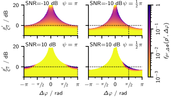
Figure 4: Joint probability functions of $P^{\prime}$ and IPD as defined in Eq. (15). The panels show functions for different SNRs and Tone-IPDs $\psi$. The horizontal dashed black lines indicate the location where $p^{\prime}=C^{2}$, the vertical black lines indicate where $\Delta\varphi=\psi$. Note that the color-map is logarithmically-scaled and that the changes in the scale were limited to values between 1 and below $10^{-3}$.

Figure 4 shows some exemplary joint PDFs of IPD and $P^{\prime}$ with the undefined region shown in white. It is notable that the probabilities are heavily clustered close to the limit defined by Eq. (18). The density in these functions decreases so quickly that a logarithmically-scaled color map had to be chosen in order to visualize the function. The limit itself is a consequence of the vector summation visualized in Fig. 1(b) and is best discussed for $\Delta\varphi=\psi$. This is obviously true for any point in time where the noise energy is zero so that the signal only contains the tone and $p^{\prime}=C^{2}$. Using geometry it can then be shown that $p^{\prime}<C^{2}$ for any other case where $\Delta\varphi=\psi$. Thus follows that $\hat{p}^{\prime}(\Delta\varphi=\pm\psi)=C^{2}$, a relation that is also visualized in form of the dotted black lines in Fig. 4. The large probability density close to the limit defined by Eq. (18) also explains the sharp peak in the marginal PDF of $P^{\prime}$ as visible in Fig. 3. From Eq. (18) follows that $\hat{p}^{\prime}(\Delta\varphi=\pm\pi)=C^{2}\sin^{2}(\nicefrac{{\psi}}{{2}})$ thus resulting in a peak around this location.

All PDFs derived in this study are independent of the noise spectrum. The spectral properties and especially the bandwidth does, however, influence the frequency of IPD, ILD and $P^{\prime}$ fluctuations. Larger bandwidths result in faster fluctuations. Further, the tone does not need to be spectrally centered in the noise. It does not even have to be within the noise spectrum. With auditory processing, especially peripheral filtering, the spectrum is of course going to influence the SNR at the level of binaural interaction and thus the PDFs of the encoded binaural cues.

While all PDFs were derived for the diotic noise case $\textup{N}_{0}\textup{S}_{\psi}$, they can easily be generalized to cases where an additional phase delay $\psi_{2}$ is applied to the whole stimulus. Such a signal could then be referred to as $(\textup{N}_{0}\textup{S}_{\psi})_{\psi_{2}}$ and would result in the same IPD distributions as in the $\textup{N}_{0}\textup{S}_{\psi}$ case but shifted by $\psi_{2}$ with ILD and $P^{\prime}$ distributions remaining unchanged.

4 Summary

Goal of this study was to derive the joint PDF for ILDs (IARs) and IPDs as well as IPDs and $P^{\prime}$. The two functions are given by the Eqs. (14) and (15). They are a key component for understanding how the SNR and $\psi$ influence the magnitude of binaural unmasking.

References

- [1] JF Culling, M Lavandier, Binaural Unmasking and Spatial Release from Masking. (Springer International Publishing), pp. 209–241 (2021).
- [2] IJ Hirsh, The influence of interaural phase on interaural summation and inhibition. The J. Acoustical Society America 20, 536–544 (1948). doi:10.1121/1.1906407.
- [3] NI Durlach, KJ Gabriel, HS Colburn, C Trahiotis, Interaural correlation discrimination: Ii. relation to binaural unmasking. The J. Acoustical Society America 79, 1548–1557 (1986). doi:10.1121/1.393681.
- [4] MJ Goupell, WM Hartmann, Interaural fluctuations and the detection of interaural incoherence: Bandwidth effects. The J. Acoustical Society America 119, 3971–3986 (2006). doi:10.1121/1.2200147.
- [5] D Just, R Bamler, Phase statistics of interferograms with applications to synthetic aperture radar. Appl.Optics 33, 4361 (1994). doi:10.1364/ao.33.004361.
- [6] GB Henning, Effect of interaural phase on frequency and amplitude discrimination. The J. Acoustical Society America 54, 1160–1178 (1973). doi:10.1121/1.1914363.
- [7] PM Zurek, Probability distributions of interaural phase and level differences in binaural detection stimuli. The J. Acoustical Society America 90, 1927–1932 (1991). doi:10.1121/1.401672.
- [8] H Levitt, EA Lundry, Binaural vector model: Relative interaural time differences. The J. Acoustical Society America 40, 1251–1251 (1966). doi:10.1121/1.1943044.
- [9] R Piessens, E de Doncker-Kapenga, CW Überhuber, DK Kahaner, Quadpack. (Springer Berlin Heidelberg), (1983).