The Last-Success Stopping Problem with Random Observation Times
Abstract
Suppose independent Bernoulli trials are observed sequentially at random times of a mixed binomial process. The task is to maximise, by using a nonanticipating stopping strategy, the probability of stopping at the last success. We focus on the version of the problem where the trial is a success with probability and the prior distribution of is negative binomial with shape parameter . Exploring properties of the Gaussian hypergeometric function, we find that the myopic stopping strategy is optimal if and only if . We derive formulas to assess the winning probability and discuss limit forms of the problem for large .
1 Introduction
Given sequentially observed independent Bernoulli trials with success probability for the trial, the last-success problem asks one to find a stopping strategy maximising the probability of stopping at the last success. The instance corresponds to the famous best-choice problem, in which the observer compares rankable items arriving in random order with the goal to stop at the best [44]. If , is a fixed number known to the observer, then the optimal strategy has a particular simple form: there exists a critical index , such that one should always skip the initial trials then stop at the first consequent success [11, 33, 32]. In this paper we will consider an instance of the following more complex setting, which generalises some previously studied best-choice problems with random and random observation times [6, 9, 10, 14, 15, 20, 26, 36, 46, 47].
Let the number of trials be governed by the distribution , called in the sequel prior, and let be a profile of success probabilities. Suppose the trials are paced randomly in time according to a mixed binomial point process with some continuous base distribution. That is to say, conditionally on the epochs of the trials are allocated like order statistics from the base distribution. The trial at the epoch is a success with probability , independently of the outcomes and epochs of all other trials. The base distribution, and are assumed to be known to the observer, who learns the times and outcomes of the trials online, aiming to stop, by means of a nonanticipating stopping strategy, at the moment of the last success. The form of the base distribution is not important, and without losing generality in the sequel we shall assume it to be -uniform.
In the best-choice problem with random observation times, a distinguished role is played by the so-called -strategy, which prescribes to skip all trials before time then stop at the first success. Bruss [8] observed that for the -strategy guarantees winning probability and that this bound is asymptotically sharp for large. However, for any fixed prior the -strategy is not optimal [29].
The analogy with many other problems of optimal stopping [24] suggests in search for the optimum to examine the myopic strategy. This strategy, denoted here , prescribes to stop as soon as the probability to win by stopping at the current trial is at least as great as the probability to win by stopping at the next success (if available). Concretely, if the trial observed at time is a success, this stopping condition holds whenever for certain cutoff . Optimality of the myopic strategy is ensured whenever the sequence of cutoffs is nonincreasing. Here is a summary of what has been known to date about the optimality of in the context of the best-choice problem:
- –
-
–
Tamaki and Wang [47] did this for the discrete uniform distribution.
- –
-
–
The problem for the negative binomial prior with integer shape parameter was first stated in [9] in terms of a mixed Poisson representation of the pacing process. The optimality of was claimed in an unpublished paper by Browne [6], but the crucial monotonicity property of the cutoffs was left without proof. The latter was settled independently in an analytic tour de force by Kurushima and Ano [36], who also used the mixed Poisson representation.
-
–
For the logarithmic series prior we have shown recently that the cutoffs are increasing, and that is not optimal and can be improved by some explicitly constructed strategies [30]. In different terms, this instance of the problem had been introduced in Bruss and Yor [16] as a way to model the observer with complete ignorance about . Bruss and Rogers [13] identified the structure of the observation process and disproved the conjecture about optimality of the -strategy.
A central theme in this paper is the last-success problem in the setting where is a negative binomial distribution with arbitrary shape parameter , and where the profile of success probabilities is
| (1) |
with another parameter . The case corresponds to the best-choice problem studied in [9] for and in [6, 36] for integer . The more general profile (1) appears in connection with a nonstationary model of the theory of records [37, 41], so from this perspective the paper falls in the area of random record models; see [7, 26, 38, 39] and Section 9.3 of this paper. For integer , the last-success problem can be interpreted as the best-choice problem with batch observations [31, 34]. Our main motivation, however, stems from connections to the broad circle of questions around the famous Ewens sampling formula [1, 22]. The latter suggests a species sampling metaphor for the following problem: given a time limit, how to stop exploring a population comprised of distinct unknown species at the very moment when the last new species is discovered?
We will show that the myopic strategy is optimal for and not optimal for , where the edge case corresponds to the logarithmic series prior. The direction of monotonicity of the cutoffs sequence changes at . The approach taken relies on properties of the Gaussian hypergeometric function (summarised in Section 9.1) that appear to be of independent interest. In the watershed case , the success epochs comprise a Poisson process and all cutoffs are equal, similarly to the instance from [9]. A counterpart of the best-choice problem treated in [6, 36] is the special case , where the relevant hypergeometric series are polynomials.
To assess the strategies with nonincreasing cutoffs, we derive a formula for the winning probability, very much in spirit of the formulas known for the full information best-choice problem [28, 43]. We also discuss some asymptotic theory for large . For the profile (1), the limit winning probability is still , achieved by a strategy with single cutoff . A more delicate limit model exploits the idea of an infinite prior, as appeared under different guises in the work on the best-choice problem [9, 10, 12, 13, 14, 30, 45, 46].
2 The problem with fixed
In this section we sketch the last-success problem where the number of trials is fixed and known to the observer [11, 30, 33, 32]. Consider first the general profile of success probabilities, with and for . The number of successes among trials has the Poisson-binomial distribution with probability generating function
In particular, the probability of zero successes is
| (2) |
and the probability of one success is
| (3) |
where and . Since the sum decreases in there exists a threshold such that the inequality
holds for . It follows as in the classic best-choice problem [23] that the optimal strategy of the observer knowing is to stop at the first success among trials (or to not stop at all if none of these trials is a success). The function is unimodal in , with maximum achieved at the threshold value , see [11, 30, 33, 41, 32] for more details including asymptotics and bounds.
It is also useful to inspect the dependence on . As grows, both and the maximum value are nonincreasing, provided (this condition certainly holds if ), see [30]. Moreover, we have:
Lemma 1.
The function is unimodal in the variable .
Proof.
Using (3) and manipulating the sums gives
Since the expression in brackets decreases in , the left-hand side has at most one change of sign from to . ∎
Now, we specialise the success profile to (1). The distribution of the number of successes among trials has a nice probability generating function
| (4) |
where denotes the Pochhammer factorial. The instance is sometimes called the Karamata-Stirling law [5]. From (4), for the probability of zero and one successes becomes, respectively,
The threshold is found from the double inequality
| (5) |
in full analogy with the classic case [23].
As , the logarithmic approximation to the harmonic series yields via (5) the limits
| (6) |
Thus the limiting winning probability is regardless of , but the proportion of trials skipped before being willing to stop on a success depends on the parameter.
3 Myopic and other strategies in the general setting
Consider the general prior and profile . Let be independent random variables, with ’s being uniform- and . Define a mixed binomial process
with chronologically ordered epochs . That is, given (for ) the epochs coincide with the order statistics of . With each we associate a Bernoulli trial resulting in success with probability , independently of anything else. We let undefined on the event .
We speak of state to designate the event . Similarly, under state (for ) we mean that the time of trial with index is and that the trial is a success. Being a subsequence of , the bivariate sequence of success trials increases in both components. The generic success trial can also be denoted as , meaning that is some unspecified and the observed trial is a success.
Using the term ‘state’ is justified by the fact that the sequence of success trials is Markovian, because is all what we need to know to make inference about the number of trials after time and their outcomes. Formally, let be the natural filtration, where the -algebra embraces all the information about epochs and outcomes of the trials on . Then by independence of the trials and the Markov property of mixed binomial processes [35], the distribution of the point process of epochs and outcomes of the trials on both depend on only through .
The posterior distribution of the number of trials factors as
| (7) |
where is a normalisation function. By (7) the conditional probability that there are no successes following state can be written as
| (8) |
and the probability that there is exactly one success as
| (9) |
where and are defined by (2) and (3), respectively. The adapted reward from stopping at is the conditional winning probability equal to . Likewise, the adapted reward from stopping at the next success is the probability .
Lemma 2.
For fixed , suppose . Then
-
(i)
,
-
(ii)
is nondecreasing in , and is strictly increasing if ,
-
(iii)
there exists such that for .
Proof.
Part (i) follows by checking that as .
For (ii) we first show that conditioned on stochastically increases with . To that end, consider two dependent copies of the same Markov counting process. Start at and at and let them run independently until random time , defined to be the time when the processes hit the same value, so , or if this does not occur. In the event let the processes get coupled from time on. Since both processes have only unit upward jumps, in the event , while in the event , so in any case . For this obviously gives
which is the desired stochastic monotonicity. Next, since is nondecreasing and Markovian, for the distribution of given dominates stochastically the distribution of given . Let have the first of these two distributions and the second. As is stochastically larger than , the number of successes among trials is stochastically larger than the number of successes among trials . In particular, the probability of zero successes is smaller for trials than for trials , which is . The inequality is strict if the distributions of and are distinct, which is ensured by the condition .
We define a stopping strategy to be a random variable which takes values in the random set of times and is adapted in the sense that for . The event is interpreted as not stopping at all. We shall restrict consideration to the strategies that only stop at successes . Under stopping in state we mean and that is a success epoch. For stopping at is regarded as a win if is the last success epoch.
With every ‘stopping set’ we associate a Markovian stopping strategy which stops at the first success trial with falling in . The optimal strategy exists for arbitrary and , and is Markovian by a theorem on exclusion of randomised stopping strategies (see [18], Theorem 5.3).
The myopic strategy is defined as the strategy stopping at the first state satisfying . This strategy is Markovian, with the stopping set being
| (10) |
where the cutoff is defined in Lemma 2; this is the earliest time when can accept success trial with index . If then it is not optimal to stop in the state ; but the converse is not true in general.
The so-called monotone case of the optimal stopping theory holds if is ‘closed’, meaning that after entering , the sequence of successes does not exit the set [18, 24]. This condition is necessary and sufficient for the optimality of . Since the sequence of successes is increasing in both components, this property of is equivalent to the condition , which is characteristic for the optimality of .
4 Power series priors
A distribution of can be treated within a family of power series priors
| (11) |
which share the same shape and have scale parameter varying within the radius of convergence of . A rationale for such extension is that the last-success problems are consistent for different , since the posterior distribution of in state depends on through the variable
| (12) |
Explicitly, (7) becomes
where is a normalisation function. Casting (8) and (9) as power series in , the cutoffs can be defined in terms of a sole sequence of critical roots not depending on via the formula
| (13) |
The myopic strategy is optimal for all if and only if , that is the roots are nondecreasing with .
5 The problem under the negative binomial prior
We proceed with the last-success problem for the success probabilities (1) and following the negative binomial prior with shape parameter and scale parameter .
| (14) |
The distribution increases stochastically in both and , as the formula for the mean suggests.
The pacing process has a nice structure:
Proposition 3.
Under the negative binomial prior it holds that
-
(i)
the distribution of is ,
-
(ii)
the posterior of given is ,
-
(iii)
is a Pólya-Lundberg birth process with jump rate
(15) in state ,
-
(iv)
is a mixed Poisson process with random rate distributed according to .
Proof.
Part (ii) follows from (7), (14) and the identity
The posterior mean of the number of trials on is thus
and the formula for the rate in part (ii) follows since the epochs of the trials are spread by the -uniform distribution. Part (iv) follows from the mixture representation of . Other assertions are straightforward. ∎
See [40] for summary of properties and applications of the Pólya-Lundberg process.
Let be the Gaussian hypergeometric function (commonly denoted ). The properties we need to analyse are collected in Section 9.1. It will be convenient to use interchangeably the variables and
From (4) the probability generating function of the number of successes following state becomes
where the second representation follows from the identity (26). Thus the probability of zero, respectively one successes is given by
where stands for the derivative in the first parameter of .
Complementing the general Lemma 2 we have specifically for the setting in focus:
Lemma 4.
-
(i)
is increasing in for , and decreasing in for ,
-
(ii)
is unimodal in .
Proof.
We introduce the notation and to stress that these two probabilities do not really depend on .
For , equation
becomes
| (17) |
Define to be the (unique) root of the equation on the unit interval.
Denote
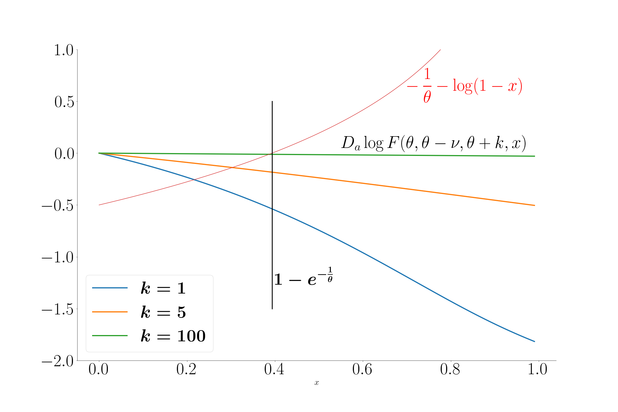
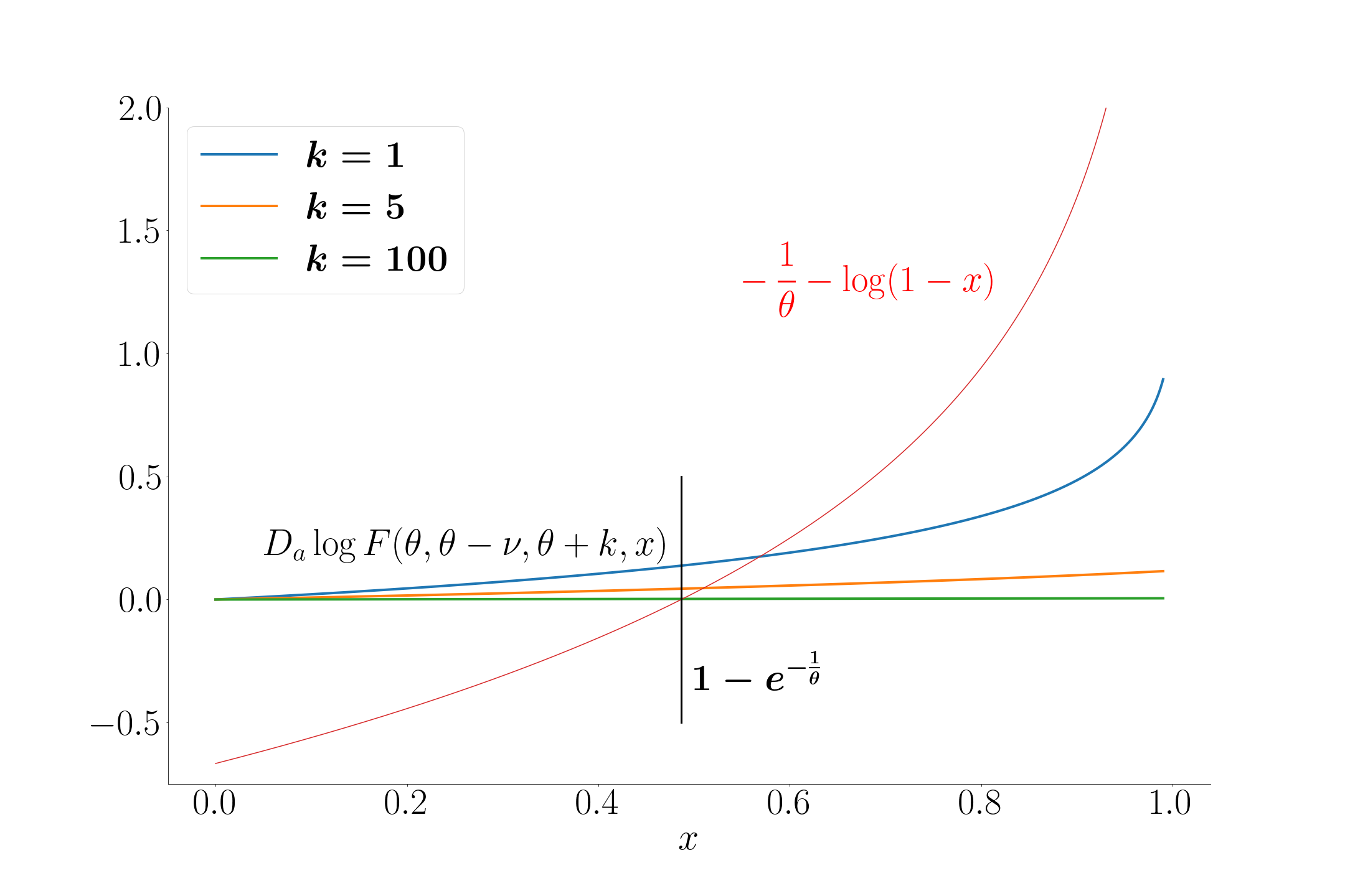
Theorem 5.
The roots satisfy
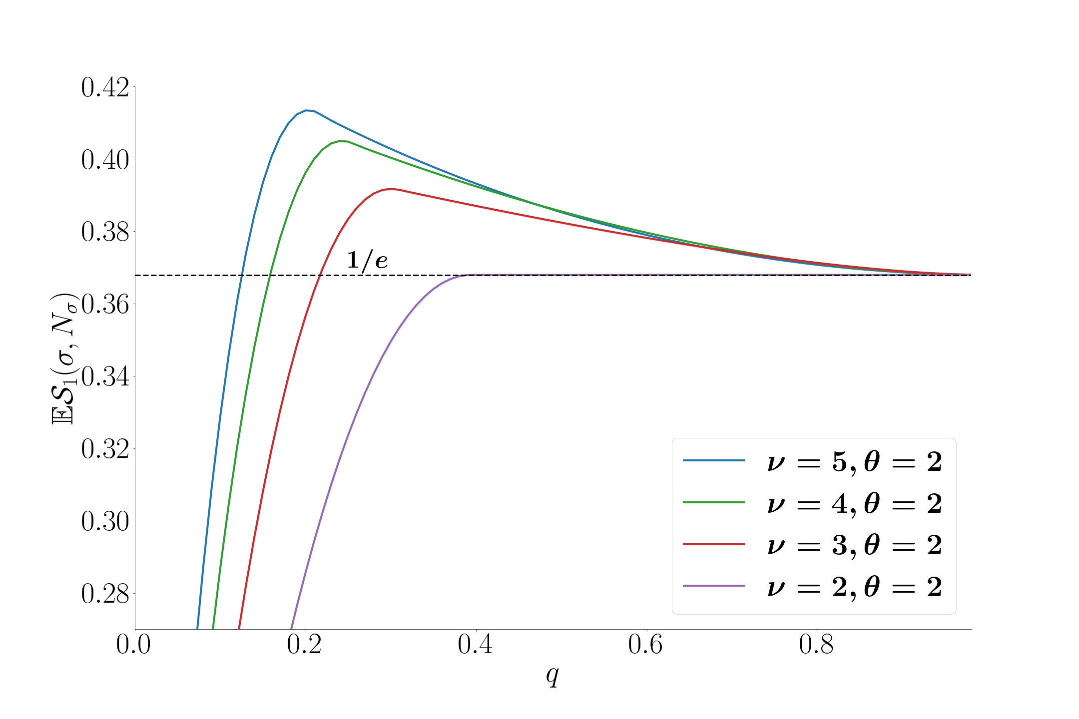
Therefore is optimal if , and not optimal if .
Proof.
Straight from the definition of by the power series (24),
This immediately implies the assertion in the case and the convergence in general.
Suppose . To justify , it is sufficient to show that
which by monotonicity of the logarithm is equivalent to
But this holds by Lemma 13.
The case is completely analogous.∎
Since the cutoffs of are related to the roots via (13), we have that ’s converge to the value . For , the myopic strategy never stops before time . For , the optimal strategy (which is not ) would stop at any success after time regardless of the index.
To contrast this result with another setting, we recall that for the best-choice problem with the Poisson prior , there are only finitely many nonzero cutoffs for each , because the analogues of ’s do not accumulate, rather grow about linearly with (see [4, 9, 20] and Section 8).
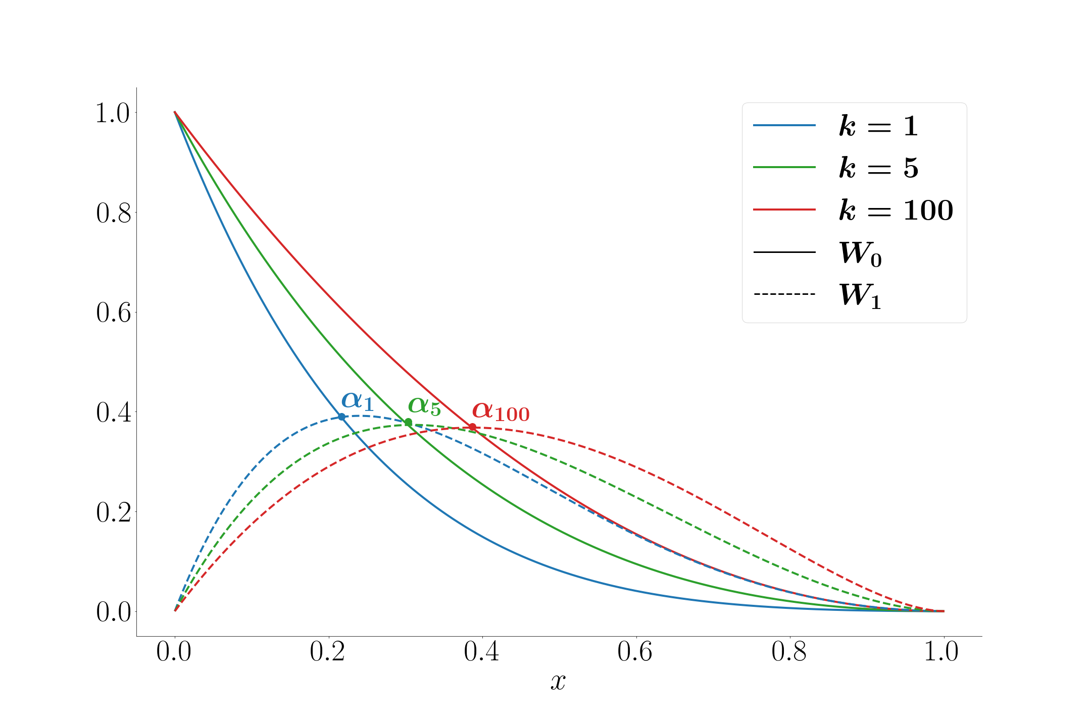
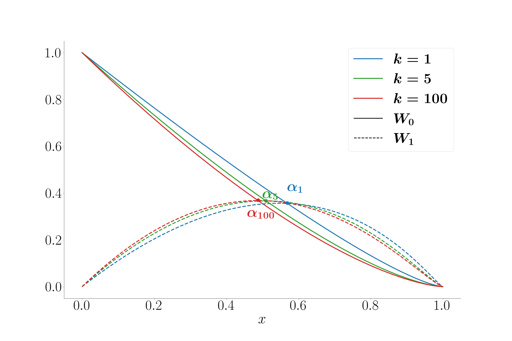
| 1 | 0.216390 | 0.568837 |
|---|---|---|
| 2 | 0.249979 | 0.537613 |
| 3 | 0.273297 | 0.523253 |
| 4 | 0.290259 | 0.515103 |
| 5 | 0.303095 | 0.50988 |
| 6 | 0.313126 | 0.506259 |
| 7 | 0.321171 | 0.503604 |
| 8 | 0.327761 | 0.501577 |
| 9 | 0.333257 | 0.499979 |
| 10 | 0.337909 | 0.498687 |
| 20 | 0.362155 | 0.492737 |
| 50 | 0.379922 | 0.489067 |
| 100 | 0.386508 | 0.487829 |
| 1000 | 0.392755 | 0.486708 |
| 10000 | 0.393398 | 0.486595 |
| 100000 | 0.393462 | 0.486584 |
| 0.393469 | 0.486583 |
The case : a Poisson process of success epochs.
In the case there is much simplification, as (LABEL:PGF1) for every becomes which is the probability generating function of the Poisson distribution with mean . All roots in this case coincide with , hence is a single cutoff strategy which skips all trials before then stops at the first success. The optimal winning probability is
hence equal to for sufficiently large (more precisely, in the range ). This generalises the result from [14] for the geometric prior.
A probabilistic reason for such simple solution is the following. From Proposition 3 (ii) and (1), the rate function for the point process of success epochs does not depend on index .
Thus, the counting process of success epochs has deterministic infinitesimal compensator, therefore the process is Poisson by Watanabe’s martingale characterisation. So the last-success problem in this case is equivalent to the elementary problem of maximising the probability of stopping at the last epoch of a Poisson process.
The polynomial case: .
If for some positive integer , the hypergeometric series (LABEL:PGF1) is a polynomial in of degree . Similarly to Jacobi polynomials ( with positive parameters) the function is representable via Rodrigues’ formula as
where denotes the th derivative in .
Showing that the roots increase in this polynomial case can be concluded by a shorter argument based on the parameter derivative formula due to Fröhlich (see Lemma 14 below),
and applying the third part of Lemma 12 to check that the right-hand side is increasing in .
The left-hand side of equation (17) for becomes increasingly more complicated with growing degree . To illustrate:
The case .
The edge case corresponds to the logarithmic series prior
| (18) |
with . Formula (LABEL:PGF1) is still valid, along with the argument for , hence is not optimal. The instance was studied in much detail in [30].
6 The winning probability
We first assume arbitrary success profile and prior . Let be a strategy with a stopping set where the cutoffs satisfy . By the monotonicity, once the process enters it stays there all the remaining time. We define the precursor associated with to be the random time
| (19) |
Clearly, and . The rationale behind this definition is that starting from time , the strategy acts greedily, by stopping at the first available success. Hence the winning probability with can be expressed as .
Both and are stopping times adapted to the filtration but, as the next lemma shows, takes values in a larger set .
Lemma 6.
for holds iff either
-
(i)
, in which case ,
or
-
(ii)
, in which case .
Also, is equivalent to .
Proof.
In the case (i) we have , and for it holds that hence . Thus .
In the case (ii) we have , so . On the other hand, for we have hence . Thus .
Note that the condition ‘(i) or (ii)’ means that for some . This condition is also necessary for . Indeed, if then together with would imply and ; a contradiction with (19). Likewise, if then would imply , hence choosing in the range we have , which in the view of contradicts the minimal property in (19).
In the case , only option (i) can occur. ∎
Remark
On the event the precursor is
This has a nice combinatorial interpretation. The cutoffs split into compartments, where the points are allocated. The sequence of cluster sizes can be written in stars and bars notation, like for instance for . The precursor corresponds to the symbol (star or bar) in this sequence.
The winning probability can be computed by conditioning on the number of trials as
| (20) |
The formula is valid for arbitrary and . To apply (20) one needs to find the distribution of given trials.
Lemma 7.
For , we have
where .
Proof.
The case is easy: . For , by Lemma 6, the event occurs if either or falls in , hence
and the asserted formula follows. ∎
Formula (20) resembles known formulas for the winning probability in the full-information best-choice problem [28, 43]. Alternatively, a direct application of Lemma 6 yields
| (21) |
7 Asymptotics and limit forms of the problem
7.1 Asymptotic optimality
For profile (1), there is a universal asymptotics valid under the sole assumption that the number of trials becomes large.
Proposition 8.
As (in probability), the strategy with single cutoff stops at the last success with probability approaching , which is the asymptotically optimal winning probability.
Proof.
Condition on , with large. By the second limit relation in (6) the winning probability cannot exceed , even if the observer knows apriori. Hence is an asymptotic upper bound.
On the other hand, it is still true that for converging in probability to , as . By the law of large numbers, this holds for , the count of trials before time . Therefore the strategy with single cutoff has the winning probability converging to . ∎
In fact, there are many Markovian asymptotically optimal strategies.
Proposition 9.
Let be a strategy with cutoffs . If and then is asymptotically optimal as (in probability).
Proof.
Let be the strategy with cutoff . We argue that the equality holds with probability approaching one. Indeed, the least cutoff is strictly positive. Fix small and choose such that for . If then unless there is a success epoch in the -vicinity of . As also and the probability that there exists such is of the order (see the next proposition). ∎
7.2 A Poisson limit problem
More insight in the asymptotics is gained by looking at the temporal pattern of success trials. Let be a nonhomogeneous Poisson point process with rate function , . This is the familiar selfsimilar Poisson process [42] restricted to the unit interval. Note that has infinitely many points and these accumulate near .
Proposition 10.
As (in probability), the point process of success epochs converges weakly to .
Proof.
Condition on , for large. The approximation of the point process of success epochs by works for trials occurring at fixed times since and , see [41]. This is readily extended to the mixed binomial process by noting that by the law of large numbers the process converges weakly to the identity function. ∎
The following last-arrival problem can be seen as a limit form of the last-sucess problem. Suppose the points of are revealed in their natural order with the objective to stop at the last point before time . The optimal strategy is then to stop at the first point after time . The optimality is justified by a standard monotone case argument, with the cutoff found by equating the probability of zero Poisson points on and the probability of exactly one such point. For , this limit form is a special case of the Gianini and Samuels [27] infinite secretary problem.
7.3 Infinite priors
By the virtue of Proposition 3, the last-success problem with negative binomial prior can be formulated straight in terms of the Pólya-Lundberg process starting from , that is with the initial state . The optimal strategy is characterised by some stopping set of states . If we consider the pacing process starting from any other initial state , the optimal strategy will be to stop at the first subsequent success with . In this sense the optimal strategy does not depend on the initial state. This follows from the optimality principle and the fact that every state is reachable from . Likewise, the myopic strategy is determined by the stopping set as in (10) regardless of the initial state of the pacing process.
Let be the strategy with cutoffs . By Proposition 9 this strategy is asymptotically optimal. In particular, is asymptotically optimal under the negative binomial prior as . We aim to confer to yet another sense of optimality in the case .
To that end, note that for initial state with the Pólya-Lundberg process with rates formula (15) is well defined also for . The case must be excluded because the rate function has a pole at . In this setting, is the myopic strategy whose winning probability depends on and converges to as . If , strategy is optimal in the last-success problem with any such initial state.
The setting can be interpreted as the last-success problem with infinite prior
| (22) |
Although this is not a probability distribution, a formal Bayes calculation of the posterior for given (with ) yields the proper negative binomial distribution , in accord with part (ii) of Proposition 3. Exactly this distribution of emerges under the Pólya-Lundberg process with parameter and initial state .
For the best-choice problem () with the idea of formal Bayes optimality was introduced by Stewart [46], who proved the optimality of the -strategy (which coincides with in this case). For , (22) is the uniform distribution on nonnegative integers, regarded in the statistical literature as ‘noninformative prior’ to address the situation of complete ignorance about the value of . Bruss [20] considered the best-choice problem with mixed Poisson pacing process whose rate was assumed to follow the infinite uniform distribution on positive reals, however it is not hard to see that this setting is equivalent to that of [46]. Thus the -strategy is both Bayes optimal under the infinite uniform prior and optimal in the limit model of Section 7.2 (see discussion in [14], p. 829). But note that in our two parameter framework the latter applies to only if .
The edge case of (22) corresponds to the infinite logarithmic series prior , which is the analogue of (18). In different terms, the model was proposed in [16] as yet another way to model the complete ignorance about . Bruss and Rogers [13] observed that the pacing process is a birth process and showed that the -strategy is not optimal in the best-choice problem with initial state , . To this we can add that the monotone case of optimal stopping fails for every , thus neither myopic nor any single cutoff strategy is optimal for initial states .
8 A unified Markovian approach
A simple time change allows us to embed the last-success problems with different in a unified framework of a single Markov process. Parameter will assume the role of the initial state. Consider the general power series prior (11), and let be the maximal convergence interval of . If for some then there exists an improper prior . The latter does not apply, for instance, to the shapes like or .
The associated mixed binomial process has the property that the conditional distribution of given depends on and through . Thus the process , with the temporal variable decreasing from to , has a jump rate not depending on . Let be a Markov process with the state space and the transition kernel defined by
The process starting from has the same distribution as . Suppose state of is marked as success with probability , independently of anything else. The last-sucess problem with parameter translates as the optimal stopping of starting from state .
A Markovian stopping strategy in this setting is determined by a subset of . Denote the maximum winning probability achievable by proceeding from state , the probability of no successes following the state and let . The optimal strategy by starting from any given is to stop at the first state in which is marked as success. This very set corresponds to the Bayes optimal strategy whenever the infinite prior exists.
Specialising to the negative binomial prior (14) (with fixed) we have , ,
| (23) |
Similarly to [30], the value function satisfies the optimality equation
with the initial condition . Conditioning on the time of the first subsequent trial yields an equivalent integro-differential equation
The role of the boundary condition at ‘’ is played by the asymptotics
which follows from Proposition 10.
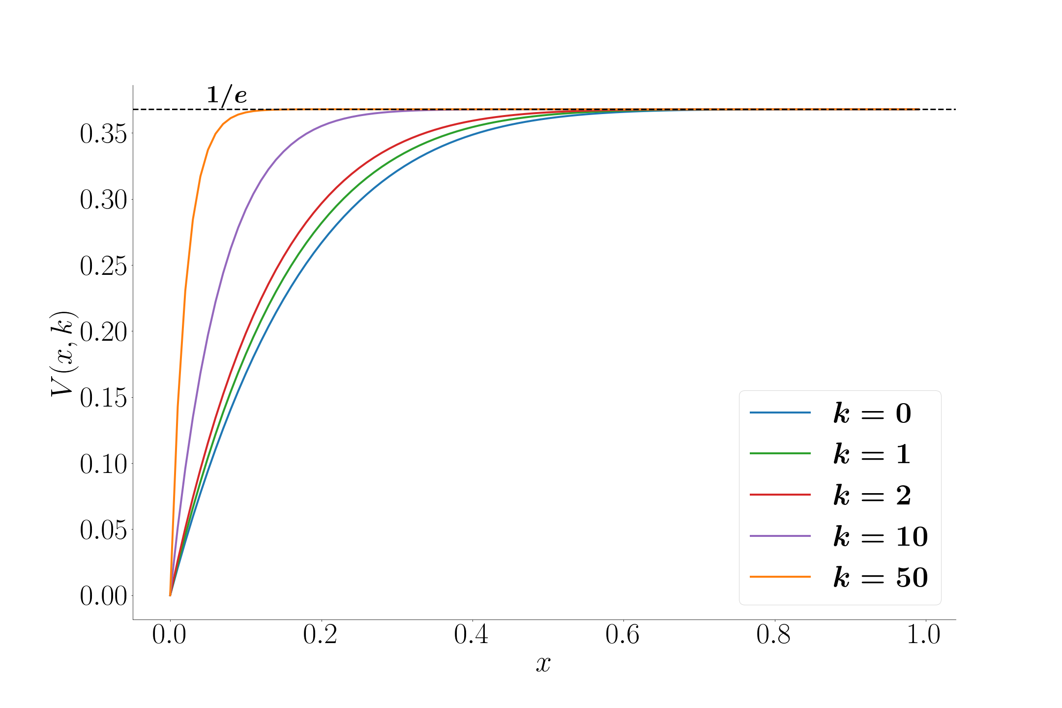
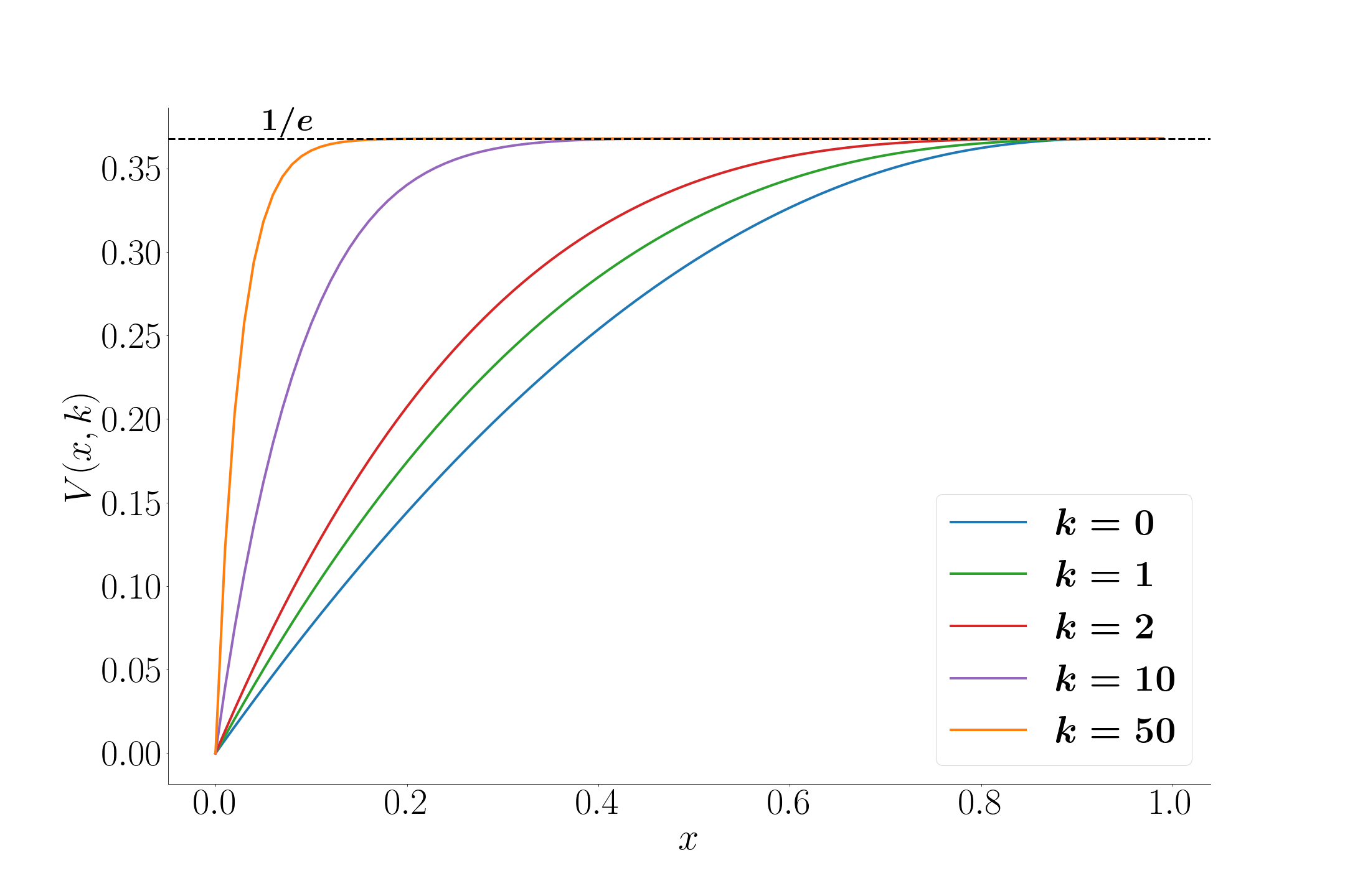
Some conclusions about the value function can be drawn from what we know about the optimal strategy. For , we have hence the optimal strategy stops greedily for and in this range we have . For , from Theorem 5 we have if ; and since it is never optimal to stop for we have a relation
where ’s are the masses of .
Remark
To revisit another known example, suppose and , so is the Poisson process with rate . In this case the rate function for is constant . From [20] we know that the optimal stopping set is of the form (23), where is the positive root of the equation
and that the sequence of roots is strictly increasing. Therefore the optimal strategy coincides with the myopic strategy. Unlike the negative binomial case, the roots do not converge, rather have asymptotics which was observed in [19]. The convergence interval of is and the ‘infinite Poisson prior’ does not exist.
9 Appendix
9.1 The hypergeometric function
This section collects monotonicity properties of the Gaussian hypergeometric series
| (24) |
viewed as a function of real parameters and . We shall use standard formulas
| (25) | |||||
| (26) | |||||
| (27) |
and Euler’s integral representation
| (28) |
Lemma 11.
For positive and
Proof.
For the assertion is obvious from the monotonicity of and the series formula of the hypergeometric function.
Lemma 12.
For , we have the sign identities:
and
Lemma 13.
For and
Proof.
If the second parameter is a negative integer, is a polynomial. In this case there is a formula for due to Fröhlich [25]:
Lemma 14.
For a positive integer,
9.2 Baskakov’s operator
The operator associating with sequence the function
is one of Baskakov’s operator from the interpolation theory, see Equation (6) in [2].
Lemma 15.
If is unimodal then is unimodal too.
Proof.
A lengthy calculation yields the derivative
By unimodality of , the coefficients of the power series have at most one variation of sign, By Descarte’s rule of signs [21] has at most one positive root, hence is unimodal on .
∎
9.3 Nevzorov’s model for records
This section gives some motivation for (1) by way of the theory of records. Recall the following well known fact. For i.i.d. random variables with continuous distribution, the indicators of maximal records are independent and satisfy . Nevzorov’s model is a generalisation to the nonstationary case.
For continuous distribution function , let be independent with
where are given positive constants. Then the indicators are independent with
see [37] (Lecture 25). A special choice of constants yields the profile (1).
Proposition 16.
The profile of indicators is (1) for
and this is the only choice of ’s up to a constant positive multiple.
Proof.
This is shown by induction with the aid of the mean-value recursion
∎
For integer, is integer too. In that case the last-success problem has interpretation as the best-choice problem with ‘group interviewing’, where at stage the choice can be made from items sampled without replacement from a population of rankable individuals. For large number of groups this model is asymptotically simiar to the case considered in [41].
Hofman in [48] applied Nevzorov’s model for records to the best choice problem where arrivals are Poissonian with unknown intensity. However, monotonicity has been stated without proof.
References
- [1] Arratia, R., Barbour, A.D. and Tavaré, S. Logarithmic combinatorial structures: a probabilistic approach, Eur. Math. Soc., 2003.
- [2] Baskakov, V. A. (1957) An example of a sequence of linear positive operators in the space of continuous functions. Doklady Akademii Nauk SSSR 113 249–251.
- [3] Bateman, H. and Erdelyi, A. Higher transcendental functions, vol. 1, Mc Graw-Hill, NY, 1953.
- [4] Berezovsky, B.A. and Gnedin, A. V. The best choice problem, Moscow, Nauka, 1984.
- [5] Bingham, N.H. Tauberian theorems for Jakimovski and Karamata-Stirling methods. Mathematika 35(2), 1988.
- [6] Browne, S. (1993) Records, mixed Poisson processes and optimal selection: an intensity approach, Columbia University, preprint.
- [7] Browne, S. and Bunge, J. (1995) Random record processes and state dependent thinning. Stochastic Process. Appl. 55, 131–142.
- [8] Bruss, F.T. (1984) A unified approach to a class of best choice problems with an unknown number of options. Ann. Probab. 12, 882–889.
- [9] Bruss, F. T. (1987) On an optimal selection problem of Cowan and Zabczyk. J. Appl. Probab. 24, 918–928.
- [10] Bruss, F. T. (1988) Invariant record processes and applications to best choice modelling. Stochastic Process. Appl. 30, 303–316.
- [11] Bruss, F. T. (2000) Sum the odds to one and stop. Ann. Probab. 28, 1384–1391.
- [12] Bruss, F. T. and Rogers , L. C. G. (1991) Embedding optimal selection problems in a Poisson process. Stochastic Process. Appl. 38, 267–278.
- [13] Bruss, F. T. and Rogers , L. C. G. (2021) The -strategy is sub-optimal for the problem of best choice under no information. Stoch. Process. Appl.
- [14] Bruss, F. T. and Samuels, S. M. (1987) A unified approach to a class of optimal selection problems with an unknown number of options. Ann. Probab. 15, 824–830.
- [15] Bruss, F. T. and Samuels, S. M. (1990) Conditions for quasi-stationarity of the Bayes rule in selection problems with an unknown number of rankable options. Ann. Probab. 18, 877–886.
- [16] Bruss, F. T. and Yor, M. (2012) Stochastic processes with proportional increments and the last-arrival problem. Stochastic Process. Appl. 122, 3239–3261.
- [17] Bunge, G. and Goldie, C.M. (2001) Record sequences and their applications, in: Handbook of Statistics, D.N. Shanbhag and C.R.Rao eds. 19, 277–308.
- [18] Chow, Y.S., Robbins, H. and Siegmund, D. The theory of optimal stopping, Dover, 1991.
- [19] Ciecielski, Z. and Zabszyk, J. (1979). A note on a selection problem. Probability Theory, Banach Center Publications 5 47–51.
- [20] Cowan, R. and Zabczyk, J. (1978) An optimal selection problem associated with the Poisson process. Theory Probab. Appl. 23, 584–592.
- [21] Curtiss, D. R. (1918) Recent extensions of Descartes’ rule of signs, Ann. Math. 19, 251–278.
- [22] Crane, H. (2016) The ubiquitous Ewens sampling formula. Statist. Sci. 31, 1–19.
- [23] Dynkin, E.B. and Yushkevich, A.A., Markov Processes: theorems and problems, Plenum Press, 1969.
- [24] Ferguson, T.S. (2008) Optimal stopping and applications, https://www.math.ucla.edu/ tom/Stopping/Contents.html
- [25] J. Fröhlich (1994), Parameter derivatives of the Jacobi polynomial and the Gaussian hypergeometric function, Integral Transforms and Special Functions 2, 253–266.
- [26] Gaver, D. P. (1976) Random record models. J. Appl. Probability 13, 538–547.
- [27] Gianini, J. and Samuels, S. (1976) The infinite secretary problem. Ann. Probab. 4, 418–432.
- [28] Gilbert, E. and Mosteller, F. (1966) Recognizing the maximum of the sequence. J. Am. Statist. Assoc. 61, 35–73.
- [29] Gnedin, A. (2022) The random arrivals problem: how to beat the -strategy of the best choice, Stochastic Process. Appl. 145, 226–240.
- [30] Gnedin, A. and Derbazi, Z. (2022) Trapping the ultimate success, Mathematics 10, doi.org/10.3390/math10010158
- [31] Govindarajulu, Z. (1992) The secretary problem with batch interviewing and cost, RAIRO-Operations Research 26 (4), 391–407.
- [32] Grau Ribas, J.M. (2020) A note on last-success-problem, Theory Probab. Math. Stat. 103, 155–165.
- [33] Hill, T.P. and Krengel, U. (1992) A prophet inequality related to the secretary problem, Contemporary Mathematics 125, AMS, pp. 209-216.
- [34] Hsiau, S.-R. and Yang, J.-R. (2000) A natural variation of the standard secretary problem, Statistica Sinica 10, 639–646.
- [35] Kallenberg, O. Random measures, Springer 2017.
- [36] Kurushima, A. and Ano, K. (2003). A Poisson arrival selection problem for Gamma prior intensity with natural number parameter. Sci. Math. Japon. 57, 217–231.
- [37] Nevzorov, V. Records: mathematical theory (Lecture 25), Translation of Mathematical Monographs 194, AMS, 2001.
- [38] Orsingher, E. (1980) Extreme values of a sequence of random variables associated with the linear birth and Pólya process. Biom. Praxim. 2, 47–58.
- [39] Orsingher, E. and Battaglia, F. (1979). Record values in Poisson and randomized Poisson models, Publ. Inst. Stat. Univ. Paris 24, fasc. 3-4, 69–78.
- [40] Pfeifer, D. Pólya-Lundberg process, In: Kotz, S. et al (eds) Encyclopedia of statistical sciences vol. 1, Wiley 2006.
- [41] Pfeifer, D. (1989) Extremal processes, secretary problems and the law, J. Appl. Probab. 26 722–733.
- [42] Pitman, J. and You, Z. (2021) The range of a self-similar additive gamma process is a scale invariant Poisson point process, arxiv.org/abs/2111.09409
- [43] Porosiński, Z. (1987) The full-information best choice problem with a random number of observations, Stat. Prob. Letters 56, 419–423.
- [44] Samuels, S.M. Secretary problems. in: Handbook of Sequential Analysis (B.K. Ghosh and P.K. Sen eds), 381–402, Statist. Textbooks Monogr., 118, Dekker, New York, 1991.
- [45] Sakaguchi, M. (1989) Some infinite problems in classical scretary problems. Math. Jap. 34, 307–318.
- [46] Stewart, T. J. (1981) The secretary problem with an unknown number of options. Oper. Res. 29, 130–145.
- [47] Tamaki, M. and Wang, Q. A random arrival time best-choice problem with uniform prior on the number of arrivals. In:Optimization and Optimal Control, Chinchuluun, A., et al. eds, pp. 499–510. Springer Optim. Appl. 39, 2010.
- [48] Hofmann, G. , A Family of General Record Models, Doctoral dissertation, The Ohio State University, 1997