Topological Theory of Phase Transitions

Abstract

The investigation of the Hamiltonian dynamical counterpart of phase transitions, combined with the Riemannian geometrization of Hamiltonian dynamics, has led to a preliminary formulation of a differential-topological theory of phase transitions. In fact, in correspondence of a phase transition there are peculiar geometrical changes of the mechanical manifolds that are found to stem from changes of their topology. These findings, together with two theorems, have suggested that a topological theory of phase transitions can be formulated to go beyond the limits of the existing theories. Among other advantages, the new theory applies to phase transitions in small $\displaystyle N$ systems (that is, at nanoscopic and mesoscopic scales), and in the absence of symmetry-breaking. However, the preliminary version of the theory was incomplete and still falsifiable by counterexamples. The present work provides a relevant leap forward leading to an accomplished development of the topological theory of phase transitions paving the way to further developments and applications of the theory that can be no longer hampered.

I Introduction

Phase transitions phenomena are ubiquitous in nature at very different scales in space and in energy. Therefore, from the theoretical viewpoint, understanding their origin, and the way of classifying them, is of central interest. In spite of a huge literature on this topic, a general theory is still lacking. In the framework of Landau’s phenomenological theory, phase transitions are generally related to the mechanism of spontaneous symmetry breaking. However, Landau’s theory is not all-encompassing. Indeed, many systems do not fit in this theory and undergo a phase transition lacking spontaneous symmetry breaking and lacking an order parameter. Some notable examples are : Kosterlitz-Thouless transitions after Mermin-Wagner theorem, systems with local gauge symmetries after Elitzur’s theorem, liquid-gas transitions, transitions in supercooled glasses and liquids, transitions in amorphous and disordered systems, folding transitions in homopolymers and proteins. Furthermore, to account for the loss of analyticity of thermodynamic observables, the mathematical description of phase transitions requires the limit of an infinite number of particles (thermodynamic limit) as is the case of the Yang-Lee theory YL and of the Dobrushin-Lanford-Ruelle theory DLR . However, the contemporary research on nanoscopic and mesoscopic systems, on the biophysics of polymers bachmann ; PRL-Bachmann , on Bose-Einstein condensation, Dicke superradiance in microlaser, superconducting transitions in small metallic objects, tackles transition phenomena in systems of finite - and often very small - number of particles.

Within all the hitherto developed theoretical frameworks, also including the monumental theory of Renormalization Group and critical phenomena, it is assumed that the primitive object at the grounds of a theory is a given statistical measure; schematically: the gran-canonical measure in the old Yang-Lee theory, the canonical measure in the Dobrushin-Lanford-Ruelle theory, and the microcanonical measure in a still somewhat open and more recent approach gross ; bachmann ; PRL-Bachmann . However, there are several general results suggesting that the possibility for a system to undergo a phase transition depends on some measure-independent properties, as is its spatial dimension, the dimensionality of its order parameter, the range of its interactions, the symmetry group (discrete or continuous) of its Hamiltonian. This hints at the possibility that the same information might be encoded already at a more fundamental level completely determined by the internal interactions of a system, interactions described by their potential function.

Therefore, looking for generalisations of the existing theories is a well motivated and timely purpose. The present paper puts forward a new starting point for a line of thought initiated several years ago and based on a variety of results which hitherto did not appear to fit in a coherent theoretical framework. The central idea of this line of thought is that the singular energy dependence of the thermodynamic observables at a phase transition is the ”shadow” of some adequate change of topology of the energy level sets in phase space (or of the potential level sets in configuration space, as well).

I.1 Why topology

Recently, the study of equilibrium phase transitions in the microcanonical ensemble has attracted increasing interest, being very important in presence of ensemble inequivalence, when only the microcanonical ensemble gives the correct results. Two complementary approaches have been undertaken. One of these is of a statistical kind gross ; bachmann , recently summarized in a very interesting, powerful and rich classification of microcanonical phase transitions by M.Bachmann in Ref.PRL-Bachmann . On another side, as the ergodic invariant measure of nonintegrable Hamiltonian systems is the microcanonical measure, the other approach resorts to the study of Hamiltonian dynamics of systems undergoing phase transitions. This dynamical approach brings about interesting novelties with respect to the standard studies of phase transitions, eventually leading to the Topological Hypothesis (TH) through the following logical chain. The dynamics of a generic system of $\displaystyle N$ degrees of freedom described by a Hamiltonian $\displaystyle H=\frac{1}{2}\sum_{i=1}^{N}p_{i}^{2}+V(q_{1},\ldots,q_{N})\leavevmode\nobreak\ ,$ or equivalently by the corresponding Lagrangian function $\displaystyle L=\frac{1}{2}\sum_{i=1}^{N}{\dot{q}}_{i}^{2}-V(q_{1},\ldots,q_{N})\leavevmode\nobreak\ ,$ is chaotic. The degree of chaoticity of the dynamics is measured by the largest Lyapunov exponent, a new observable that has been proven useful to characterize phase transitions from a dynamical viewpoint book . Then, the explanation of the origin of Hamiltonian chaos - encompassing the computation of the largest Lyapunov exponent - proceeds by identifying a Hamiltonian flow with a geodesic flow of an appropriate Riemannian differentiable manifold. This differential geometric framework is given by configuration space endowed with the non-Euclidean metric of components marco $\displaystyle g_{ij}=2[E-V(q)]\delta_{ij}$, whence the infinitesimal arc element $\displaystyle ds^{2}=2[E-V(q)]^{2}dq_{i}\ dq^{i}$; then Newton equations are retrieved from the geodesic equations

$$\frac{d^{2}q^{i}}{ds^{2}}+\Gamma^{i}_{jk}\frac{dq^{j}}{ds}\frac{dq^{k}}{ds}=0\ ,$$

where $\displaystyle\Gamma^{i}_{jk}$ are the Christoffel connection coefficients of the manifold. The degree of instability of the dynamics is described by means of the Jacobi–Levi-Civita equation for the geodesic spread

$$\frac{\nabla^{2}J}{ds^{2}}+R(J,\dot{\gamma})\dot{\gamma}=0\ ,$$

where the vector field $\displaystyle J$ locally measures the distance between nearby geodesics, $\displaystyle\frac{\nabla}{ds}$ is the covariant derivative along the configuration space geodesic $\displaystyle{\dot{\gamma}}$, and $\displaystyle R(\cdot,\cdot)$ is the Riemann curvature tensor. The largest Lyapunov exponent for high dimensional Hamiltonian flows is found to depend on the curvature “landscape” of the configuration space manifold book . Hence, a natural consequence has been to investigate whether the occurrence of phase transitions has some peculiar counterpart in geometrical changes of the manifolds underlying the flows. And it has been discovered that this is actually the case. Moreover, the peculiar geometrical changes associated with phase transitions were discovered to be the effects of deeper topological changes of the potential level sets $\displaystyle\Sigma_{v}^{V_{N}}:=\{V_{N}(q_{1},\dots,q_{N})=v\in{\mathbb{R}}\}$ in configurations space, and, equivalently, of the balls $\displaystyle\{M_{v}^{V_{N}}=V_{N}^{-1}((-\infty,v])\}_{v\in{\mathbb{R}}}$ bounded by the $\displaystyle\Sigma_{v}^{V_{N}}$.

A topological approach to the study of phase transitions has been considered for a variety of systems, ranging from those undergoing entropy driven transitions carlsson1 ; barish (having also applications to robotics), and hard spheres systems mason , to quantum phase transitions brody ; BFS ; volovik , glasses and supercooled liquids angelani ; stillinger , classical models in statistical mechanics risau ; schilling ; fernando , discrete spin models cimasoni , DNA denaturation grinza , peptide structure becker , to quote just a few of them. In fact, in many contexts, well before an explicit formulation of the TH CCCP ; CCCPPG , topological concepts were implicitly entering the study of phase transitions while talking of energy landscapes brooks ; wales and of saddle points for disordered systems, glasses angelani ; stillinger , spin glasses: saddle points being critical points in the language of Morse theory of differential topology.

On a completely different field, more recently, handling Big Data - outsourcing from complex systems - through methods referred to as Topological Data Analysis (TDA) it happens to highlight the existence of phase transition-like phenomena in the absence of a statistical measure. Here the concept of phase transition is intended as the emergence of qualitatively new properties when a control parameter crosses a critical value (the prototype can be dated back to the Erdös-Renyi giant component appearance in random graphs). To quote a fascinating example in this field, in Ref.brain the discovery is reported of topological phase transitions in functional brain networks by merging concepts from TDA, topology, geometry, physics, and network theory.

The present paper is organized as follows: in Section II the basic definitions and concepts of extrinsic geometry of hypersurfaces is recalled for the sake of self-containedness, and the definition of asymptotic diffeomorphicity is also therein introduced. In Section III the Main theorem is formulated and proved; this theorem states that a topological change of the potential level sets of a physical system is a necessary condition for the appearance of a phase transition. Finally, in Section IV the problem raised by the counterexample to a preceding formulation of the Main theorem is fixed. Section V is devoted to some concluding remarks, two appendices contain computational details, and a third appendix addresses some past controversial points.

II Topological origin of phase transitions

On the one side the study of the Hamiltonian dynamical counterpart of phase transitions, combined with the geometrization of Hamiltonian dynamics, has led to find out the crucial role of topology at the grounds of these transition phenomena, on the other side a mathematical relationship exists between macroscopic thermodynamics and topological properties of the manifolds $\displaystyle M_{v}^{V_{N}}$, as expressed by book

$$S_{N}(v)=({k_{B}}/{N})\log\left[\int_{M_{v}^{V_{N}}}\ d^{N}q\right]=\frac{k_{B}}{N}\log\left[vol[{M_{v}^{V_{N}}\setminus\bigcup_{i=1}^{{\cal N}(v)}\Gamma(x^{(i)}_{c})}]\ +\sum_{i=0}^{N}w_{i}\ \mu_{i}(M_{v}^{V_{N}})+{\cal R}\right],$$ (1)

where $\displaystyle S_{N}$ is the configurational entropy, $\displaystyle v$ is the potential energy, and the $\displaystyle\mu_{i}(M_{v}^{V_{N}})$ are the Morse indexes (in one-to-one correspondence with topology) of the manifolds $\displaystyle M_{v}^{V_{N}}$; in square brackets: the first term is the result of the excision of certain neighborhoods of the critical points of the interaction potential from $\displaystyle M_{v}^{V_{N}}$; the second term is a weighed sum of the Morse indexes, and the third term is a smooth function of $\displaystyle N$ and $\displaystyle v$.

Figure 1: Low-dimensional pictorial representation of the transition between complex topologies as a metaphor of the origin of a phase transition. From the ground level up to the crossover level $\displaystyle v_{c}$, the manifolds $\displaystyle M_{v}$ have a genus which increases with $\displaystyle v$. Above the crossover level $\displaystyle v_{c}$, the manifolds $\displaystyle M_{v}$ have also a nonvanishing linking number which increases with $\displaystyle v$.

As a consequence, major topology changes with $\displaystyle v$ of the submanifolds $\displaystyle M_{v}^{V_{N}}$ - bringing about sharp changes of the potential energy pattern of at least some of the $\displaystyle\mu_{i}(M_{v}^{V_{N}})$ - can affect the $\displaystyle v$-dependence of $\displaystyle S_{N}(v)$ and of its derivatives.

Hence, it has been surmised book that, at least for a broad class of physical systems, phase transitions stem from a suitable change of the topology of the potential level sets $\displaystyle\Sigma_{v}^{V_{N}}$ and, equivalently, of the manifolds $\displaystyle M_{v}^{V_{N}}$, when $\displaystyle v$, playing the role of the control parameter, takes a critical value $\displaystyle v_{c}$. This hypothesis has turned into the start of a new theory by putting together several studies on specific models book ; physrep and two theorems prl1 ; NPB1 ; NPB2 . These theorems state that an equilibrium phase transition - is necessarily due to appropriate topological transitions in configuration space. However, a counterexample to these theorems has been found in Ref.kastner thus undermining this version of the topological theory of phase transitions. The counterexample is provided by the second order phase transition of the $\displaystyle 2D$ lattice $\displaystyle\phi^{4}$-model that occurs at a critical value $\displaystyle v_{c}$ of the potential energy density which belongs to a broad interval of $\displaystyle v$-values void of critical points of the potential function. The difficulty raised by this counterexample has stimulated a deeper investigation of the transition of the $\displaystyle\phi^{4}$-model which led to figure out a crucial point associated with the breaking of the $\displaystyle\mathbb{Z}_{2}$ symmetry (and possibly with the breaking of discrete symmetries in general), that is, the possibility of a phase transition to stem from an asymptotic loss of diffeomorphicity of the relevant manifolds vaff . In what follows this fact is formalized into a new and more consistent version of the theory. Other alleged difficulties of the theory are briefly discussed in Appendix C.

II.1 Basic definitions and concepts

Consider now an open set of $\displaystyle v$-values $\displaystyle I\subseteq\mathbb{R}$ such that the cylindrical subset of configuration space $\displaystyle\Gamma_{I}^{N}=\bigcup_{{v}\in{I}}\Sigma^{V_{N}}_{v}$ contains only non-singular level sets, that is, $\displaystyle\nabla V_{N}(q)\neq 0$ for any $\displaystyle q\in\Gamma^{N}_{I}$, meaning that $\displaystyle V_{N}$ has no critical points for any $\displaystyle{v}\in{I}$.

For any $\displaystyle{v}_{0},{v}_{1}\in{I}$, the two level sets $\displaystyle\Sigma^{V_{N}}_{v_{0}}\subset\Gamma^{N}_{{I}}$ and $\displaystyle\Sigma^{V_{N}}_{v_{1}}\subset\Gamma^{N}_{{I}}$ are diffeomorphic under the action of an explicitly known diffeomorphism given by the integral lines of the vector field $\displaystyle\boldsymbol{\xi}_{N}={\nabla{V}_{N}}/{\|\nabla{V}_{N}\|^{2}}$, that is, any initial condition $\displaystyle\textit{{q}}_{\alpha}\in\Sigma^{V_{N}}_{v_{0}}$ is diffeomorphically mapped onto a point $\displaystyle\textit{{q}}_{\beta}\in\Sigma^{V_{N}}_{v_{1}}$ by the equation hirsch

$$\frac{d{\textit{{q}}}}{dv}=\dfrac{\nabla{V}_{N}}{\|\nabla{V}_{N}\|^{2}}\qquad.$$ (2)

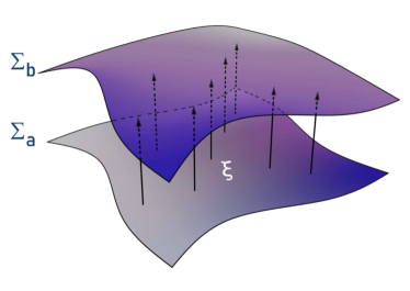
Figure 2: Pictorial representation of the action of the vector field $\displaystyle\boldsymbol{\xi}$ in Eq.(2) diffeomorphically mapping each point of the level set $\displaystyle\Sigma_{a}$ onto each point of the level set $\displaystyle\Sigma_{b}$.

II.2 Extrinsic geometry of hypersurfaces

In this section some basic definitions and concepts are given about the extrinsic geometry of hypersurfaces of a Euclidean space. The basic tool consists in measuring the way of changing from point to point on the surface of the normal direction in order to describe how the $\displaystyle n$-surface $\displaystyle\Sigma$ curves around in $\displaystyle{\mathbb{R}}^{N}$. The rate of change of the normal vector $\displaystyle{\cal N}$ at a point $\displaystyle x\in\Sigma$ in a given direction u is described by the shape operator (also known as Weingarten’s map) $\displaystyle L_{x}(\textit{{u}})=-\nabla_{\textit{{u}}}\ {\cal N}=-({\textit{{u}}}\cdot\nabla){\cal N}$, where u is a tangent vector at $\displaystyle x$ and $\displaystyle\nabla_{\textit{{u}}}$ is the directional derivative; gradients and vectors are represented in $\displaystyle{\mathbb{R}}^{N}$.

Figure 3: Illustration of the items entering the construction of the shape operator of a surface.

The constant-energy hypersurfaces in the phase space of Hamiltonian systems or of the equipotential hypersurfaces in configuration space, are the level sets of regular functions and, for the level sets defined via a regular real-valued function $\displaystyle f$ as $\displaystyle\Sigma_{a}:=f^{-1}(a)$, the normal vector is $\displaystyle{\cal N}=\nabla f/\|\nabla f\|$. Let $\displaystyle\{{\bf e}_{\mu}\}_{\mu=1,\dots,N}=\{{{\bf e}_{1},\dots,{\bf e}_{n}},{\cal N}\}$, with $\displaystyle{\bf e}_{\alpha}\cdot{\bf e}_{\beta}=\delta_{\alpha,\beta}$ and denote with Greek subscripts, $\displaystyle\alpha=1,\dots,N$, the components in the embedding space $\displaystyle{\mathbb{R}}^{N}$, and with Latin subscripts, $\displaystyle i=1,\dots,n$, the components on a generic tangent space $\displaystyle T_{x}\Sigma_{a}$ at $\displaystyle x\in\Sigma_{a}$. We consider the case of codimension one, that is, $\displaystyle N=n+1$.

From $\displaystyle\partial_{\mu}{\cal N}_{\alpha}{\cal N}_{\alpha}=0=2{\cal N}_{\alpha}\partial_{\mu}{\cal N}_{\alpha}$ we see that for any u, we have $\displaystyle{\cal N}\cdot L_{x}(\textit{{u}})=-{\cal N}_{\alpha}\textit{{u}}_{\mu}\partial_{\mu}{\cal N}_{\alpha}=0$, which means that $\displaystyle L_{x}(\textit{{u}})$ projects on the tangent space $\displaystyle T_{x}\Sigma_{a}$.

Now the principal curvatures $\displaystyle\kappa_{1},\dots,\kappa_{n}$ of $\displaystyle\Sigma_{a}$ at $\displaystyle x$ are the eigenvalues of the shape operator restricted to $\displaystyle T_{x}\Sigma_{a}$. Considering the matrix $\displaystyle{\cal L}_{x}$ to be the restriction of $\displaystyle L_{x}$ to $\displaystyle T_{x}\Sigma_{a}$

$${\cal L}_{ij}(x)={\bf e}_{i}\cdot L_{x}({\bf e}_{j})=-({\bf e}_{i})_{\alpha}({\bf e}_{j})_{\beta}\partial_{\beta}{\cal N}_{\alpha}\ ,$$

then the mean curvature is defined as

$$H(x)=\frac{1}{n}{\rm Tr}^{(n)}{\cal L}_{ij}(x)=\frac{1}{n}\sum_{i=1}^{n}\kappa_{i}\ .$$ (3)

The computation of the analytic expression of the mean curvature $\displaystyle H$ proceeds from

$$H(x)=\frac{1}{n}{\rm Tr}^{(n)}{\cal L}_{ij}(x)=-\frac{1}{n}\sum_{i=1}^{n}({\bf e}_{i})_{\alpha}({\bf e}_{i})_{\beta}\partial_{\beta}{\cal N}_{\alpha}\leavevmode\nobreak\ .$$ (4)

Defining $\displaystyle A_{\mu\nu}=({\bf e}_{\mu})_{\nu}$, so that $\displaystyle AA^{T}={\mathbb{I}}$, we have

$$\sum_{i=1}^{n}({\bf e}_{i})_{\alpha}({\bf e}_{i})_{\beta}=\delta_{\alpha\beta}-{\cal N}_{\alpha}{\cal N}_{\beta}$$

and thus

$$\displaystyle H(x)=-\frac{1}{n}(\delta_{\alpha\beta}-{\cal N}_{\alpha}{\cal N}_{\beta})\partial_{\beta}{\cal N}_{\alpha}=-\frac{1}{n}\partial_{\alpha}{\cal N}_{\alpha}=-\frac{1}{n}\nabla\cdot\left(\frac{\nabla f}{\|\nabla f\|}\right)\leavevmode\nobreak\ .$$ (5)

II.3 Asymptotic diffeomorphicity

In Ref.vaff it has been numerically found that the phase transition undergone by the $\displaystyle 2D$ lattice $\displaystyle\phi^{4}$ model actually corresponds to a major topological change of the potential level sets of the model, also in absence of critical points of the potential. This topological change corresponds to an asymptotic breaking of the topological transitivity of the potential level sets, what can be formalised as an asymptotic loss of diffeomorphicity of the same manifolds in the broken symmetry phase. Hence a crucial hint to fix the problem stemming from the counterexample given by the $\displaystyle\phi^{4}$ model that has been hitherto considered fatal.

The first step to fix the problem thus consists in defining asymptotic diffeomorphicity, what is easily done by observing that a vector valued function of several variables, $\displaystyle f:\mathbb{R}^{n}\rightarrow\mathbb{R}^{n}$, is of differentiability class $\displaystyle{\cal{C}}^{l}$ if all the partial derivatives $\displaystyle(\partial^{l}f/\partial x_{i_{1}}^{l_{1}}\dots\partial x_{i_{k}}^{l_{k}})$ exist and are continuous, where each of $\displaystyle i_{1},\dots,i_{k}$ is an integer between $\displaystyle 1$ and $\displaystyle n$ and each $\displaystyle l_{1},\dots,l_{k}$ is an integer between $\displaystyle 0$ and $\displaystyle l$, and $\displaystyle l_{1}+\dots+l_{k}=l$. Then, by taking advantage of the explicit analytic representation of the vector field generating the diffeomorphism $\displaystyle\boldsymbol{\xi}_{N}:\Gamma_{I}^{N}\rightarrow T\Gamma_{I}^{N}$ previously given, uniform convergence in $\displaystyle N$ of the sequence $\displaystyle\{\boldsymbol{\xi}_{N}\}_{N\in\mathbb{N}}$ - and thus asymptotic diffeomorphicity in some class $\displaystyle{\cal{C}}^{l}$ - can be defined after the introduction of an appropriate norm containing all the derivatives up to $\displaystyle(\partial^{l}\boldsymbol{\xi}_{N}/\partial q_{i_{1}}^{l_{1}}\dots\partial q_{i_{k}}^{l_{k}})$. At any fixed $\displaystyle N\in\mathbb{N}$, in the absence of critical points of a confining potential $\displaystyle V_{N}$, the level sets $\displaystyle\Sigma_{v}^{V_{N}}$ are non singular $\displaystyle(N-1)$-dimensional hypersurfaces in $\displaystyle\mathbb{R}^{N}$. Let us consider the already defined cylindrical subset of configuration space $\displaystyle\Gamma_{I}^{N}=\bigcup_{{v}\in{I}}\Sigma^{V_{N}}_{v}$ containing only non-singular level sets.

The lack of asymptotic breaking of diffeomorphicity is defined by introducing a norm for the $\displaystyle\boldsymbol{\xi}_{N}$ that allows to compare the diffeomorphisms at different dimensions

$$\|\boldsymbol{\xi}_{N}\|_{C^{k}(\Gamma^{N}_{{I}_{0}})}=\sup_{\textit{{q}}_{0}\in\Gamma^{N}_{{I}_{0}}}\|\boldsymbol{\xi}_{N}\|+\sum_{l=1}^{k}\sum_{\{i_{k}\}}\sum_{j=1}^{N}\|{\nabla^{l}_{\{i_{k}\}}}{\xi}_{j}\|_{\Gamma^{N}_{{I}_{0}}}$$ (6)

where $\displaystyle\{i_{k}\}$ stands for a multi-index and $\displaystyle\|{\nabla^{l}_{\{i_{k}\}}}{\xi}_{j}\|_{\Gamma^{N}_{{I}_{0}}}$ is the norm of the $\displaystyle l$-th differential operator with $\displaystyle l_{1}+\dots+l_{k}=l$

$$\|{\nabla^{l}_{\{i_{k}\}}}{\xi}_{j}\|_{\Gamma^{N}_{{I}_{0}}}=\sup_{\textit{{q}}_{0}\in\Gamma^{N}_{{I}_{0}}}\left|\dfrac{\partial^{l}{\xi}_{j}}{\partial q_{i_{1}}^{l_{1}}\dots\partial q_{i_{k}}^{l_{k}}}\right|\ .$$ (7)

The sequence of families of manifolds $\displaystyle\left\{\Gamma^{N}_{{I}_{0}}\right\}_{N\in\mathbb{N}}$ is said to asymptotically preserve the $\displaystyle C^{k}$-diffeomorphicity among the hypersurfaces $\displaystyle\Sigma_{v}^{V_{N}}$ - foliating each family - if there exists $\displaystyle B\in\mathbb{R}^{+}$ such that

$$\|\boldsymbol{\xi}_{N}\|_{C^{k}\left(\Gamma^{N}_{{I}_{0}}\right)}\leq B<+\infty\qquad\forall N\in\mathbb{N}.$$ (8)

As a consequence, from this condition we get $\displaystyle\|\nabla{V}_{N}\|=\|{\boldsymbol{\xi}}_{N}\|^{-1}\geq 1/B=C>0$ for each $\displaystyle\textit{q}_{0}\in\Gamma_{{I}_{0}}^{N}$ and all $\displaystyle N\in\mathbb{N}$, ruling out the existence of asymptotic critical points (i.e. $\displaystyle\|\nabla{V}_{N}\|\rightarrow 0$ for $\displaystyle N\rightarrow\infty$).

The analytic condition (8) entails remarkable consequences on the extrinsic geometry of the potential level sets. In fact, using $\displaystyle\sum_{i}\|X_{i}\|\geq\|\sum_{i}X_{i}\|$, from Eq. (7) at the lowest order with the aid of a normalised vector u tangent at $\displaystyle\textit{q}_{0}$ to a $\displaystyle\Sigma_{v}^{n}\subset\Gamma^{N}_{{I}_{0}}$, that is, $\displaystyle\textit{{u}}\in T_{\textit{q}_{0}}\Sigma_{v}^{n}$, we can build the quadratic forms

$$\sum_{i,j=1}^{N}\|(\partial_{i}\xi_{j})u_{i}u_{j}\|\geq\left\|\sum_{i,j=1}^{N}\left(\partial_{i}\dfrac{\partial_{j}V_{N}}{\|\nabla V_{N}\|^{2}}\right)u_{i}u_{j}\right\|$$ (9)

where $\displaystyle\partial_{i}=\partial/\partial q^{i}$. With implicit summation on repeated indices the r.h.s. of Eq.(9) is rewritten as

$$\displaystyle\left\|\left[\dfrac{1}{\|\nabla V_{N}\|}\left(\partial_{i}\dfrac{\partial_{j}V_{N}}{\|\nabla V_{N}\|}\right)+\dfrac{\partial_{j}V_{N}}{\|\nabla V_{N}\|}\partial_{i}\left(\dfrac{1}{\|\nabla V_{N}\|}\right)\right]u_{i}u_{j}\right\|$$ (10)

$$\displaystyle= \displaystyle\left\|\dfrac{1}{\|\nabla V_{N}\|}\left(\partial_{i}\dfrac{\partial_{j}V_{N}}{\|\nabla V_{N}\|}\right)u_{i}u_{j}\right\|$$

where the orthogonality, at any point $\displaystyle\textit{q}_{0}$, between the vectors u and

$\displaystyle{\cal N}=(\partial_{1}V_{N}/\|\nabla V_{N}\|,\dots,\partial_{N}V_{N}/\|\nabla V_{N}\|)$ tangent and normal to $\displaystyle\Sigma_{v}^{V_{N}}$, respectively, has been used. Through the shape operator (Weingarten map) of $\displaystyle\Sigma_{v}^{V_{N}}$ thorpe at $\displaystyle\textit{q}_{0}$

$$L_{\textit{q}_{0}}(\textit{{u}})=-L_{\textit{{u}}}{\cal N}=-(\nabla{\cal N}_{1}\cdot\textit{{u}}\ ,\dots,\nabla{\cal N}_{N}\cdot\textit{{u}})$$ (11)

the quadratic form $\displaystyle\kappa(\textit{{u}},\textit{q}_{0})=\langle\textit{{u}},L_{\textit{q}_{0}}(\textit{{u}})\rangle$ is found to coincide with the one given in Eq.(10) (last term). The quantity $\displaystyle\kappa(\textit{{u}},\textit{q}_{0})$ is known as the normal curvature of the level set $\displaystyle\Sigma_{v}^{V_{N}}$ at $\displaystyle\textit{q}_{0}$. Let $\displaystyle\{\kappa_{1}(\textit{q}_{0}),\dots,\kappa_{N}(\textit{q}_{0})\}$ denote the principal curvatures of $\displaystyle\Sigma_{v}^{V_{N}}$ at $\displaystyle\textit{q}_{0}$, with the corresponding orthogonal principal curvature directions $\displaystyle\{\textit{{v}}_{1},\dots,\textit{{v}}_{N}\}$, then the normal curvature in the direction $\displaystyle\textit{{u}}\in T_{\textit{q}_{0}}\Sigma_{v}^{N}$ is given by

$$\kappa(\textit{{u}},\textit{q}_{0})=\sum_{i=1}^{N}\kappa_{i}(\textit{q}_{0})\langle\textit{{u}},\textit{{v}}_{i}\rangle=\sum_{i=1}^{N}\kappa_{i}(\textit{q}_{0})\cos^{2}\theta_{i}$$ (12)

By choosing $\displaystyle\tilde{\textit{{u}}}\in T_{\textit{q}_{0}}\Sigma_{v}^{N}$ such that $\displaystyle\|\tilde{\textit{{u}}}\|=1$ and all the angles $\displaystyle\theta_{i}$ between $\displaystyle\tilde{\textit{{u}}}$ and $\displaystyle\textit{{v}}_{i}$ are equal to some $\displaystyle\tilde{\theta}$, we get

$$\kappa(\tilde{\textit{{u}}},\textit{q}_{0})=(\cos^{2}{\tilde{\theta}})\ \sum_{i=1}^{N}\kappa_{i}(\textit{q}_{0})=(\cos^{2}{\tilde{\theta}})\ N\ H(\textit{q}_{0})$$ (13)

where $\displaystyle H(\textit{q}_{0})$ is the mean curvature (the trace of the Weingarten map) at $\displaystyle\textit{q}_{0}$. Thus from Eqs.(10),(13) and (8)

$$\left\|\dfrac{1}{\|\nabla V_{N}\|}(\cos^{2}{\tilde{\theta}})\ N\,H(\textit{q})\right\|\leq B<+\infty\qquad\forall N\in\mathbb{N}$$ (14)

everywhere on $\displaystyle\Sigma_{v}^{V_{N}}$. Since $\displaystyle\|\nabla V_{N}\|\sim{\cal{O}}(N^{1/2})$ it follows that $\displaystyle H(\textit{q})\sim{\cal{O}}(N^{-1/2})$ everywhere on $\displaystyle\Sigma_{v}^{V_{N}}$ and uniformly in $\displaystyle N$. Therefore, the first remarkable consequence of asymptotic diffeomorphicity among the potential level sets is that their mean curvature

$$H(\textit{q})=\frac{1}{N}\sum_{i=1}^{N}\kappa_{i}(\textit{q})$$ (15)

is everywhere uniformly bounded in $\displaystyle N$. However, this does not ensure the boundedness of each principal curvature (whose sign is not definite). A-priori two or more principal curvatures of the same value but of opposite sign could diverge and mutually compensate leaving $\displaystyle H(\textit{q})$ finite. In order to get this missing information about the asymptotic boundedness of all the principal curvatures, let us consider the scalar curvature $\displaystyle{\mathscr{R}}$ of a level set $\displaystyle V(\textit{q})=v$, embedded in an Euclidean space of arbitrary dimension, which reads Zhou

$${\mathscr{R}}(\textit{q})=\frac{1}{N(N-1)}\sum_{i\leq j}^{1\dots N}\kappa_{i}(\textit{q})\kappa_{j}(\textit{q})=\frac{1}{N(N-1)}\left\{-\triangle\log\|\nabla V_{N}(\textit{q})\|+\nabla\cdot\left[\triangle V_{N}(\textit{q})\frac{\nabla V_{N}(\textit{q})}{\|\nabla V_{N}(\textit{q})\|^{2}}\right]\right\}$$ (16)

let us notice that $\displaystyle{\mathscr{R}}$ is singular at the critical points of the potential, where $\displaystyle\nabla V_{N}(\textit{q})=0$, and can be arbitrarily large in their neighborhoods; then, using $\displaystyle\|\boldsymbol{\xi}\|=\|\nabla V_{N}(\textit{q})\|^{-1}$, this can be rewritten as

$${\mathscr{R}}=\frac{1}{N(N-1)}\left\{-\triangle\log\frac{1}{\|\boldsymbol{\xi}\|}+\nabla\cdot\left[\triangle V_{N}(\textit{q})\ \boldsymbol{\xi}\right]\right\}\ ,$$ (17)

then, trivial computations (sketched in Appendix A) of the r.h.s. of this equation under the assumption of asymptotic diffeomorphicity [Eqs.(6),(7) and (8)] yield uniform boundedness also of $\displaystyle{\mathscr{R}}(\textit{q})$ entailing uniform boundedness in $\displaystyle N$ of each $\displaystyle\kappa_{i}(\textit{q})$ everywhere on each potential level set.

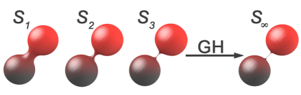
Figure 4: Sequence of diffeomorphic manifolds (of the same dimension) with a limit manifold which is not diffeomorphic to the members of the sequence. The infinitely tiny bridge between the two spheres of $\displaystyle S_{\infty}$ has infinite mean curvature.

To help intuition to get a hold of the relationship between boundedness of mean and scalar curvatures and asymptotic diffeomorphicity, we qualitatively illustrate in Figure 4 the opposite situation, known as Gromov-Hausdorff limit sormani , where a sequence of diffeomorphic manifolds of fixed dimension have a limit manifold which is not diffeomorphic to the other members of the sequence. The handles of these dumbbell shaped manifolds shrink to an asymptotic infinitely tiny cylinder of vanishing radius and thus of diverging transversal principal curvature, that is, of divergent mean curvature.

Remark 1

. Summarizing, the assumption of asymptotic diffeomorphicity means that, for any pair of densities $\displaystyle\bar{v}$ and $\displaystyle\bar{v}^{\prime}$ in some assigned interval $\displaystyle I_{\bar{v}}=[\bar{v}_{0},\bar{v}_{1}]$ and $\displaystyle N$ arbitrarily large, the corresponding manifolds $\displaystyle\Sigma_{N\bar{v}}^{V_{N}}$ are diffeomorphic under the action of the diffeomorphism-generating vector fields $\displaystyle\boldsymbol{\xi}_{N_{k}}$

$$\displaystyle\Sigma_{N_{1}\bar{v}}^{V_{N_{1}}}\quad\overset{\boldsymbol{\xi}_{N_{1}}}{\longrightarrow}\quad\Sigma_{N_{1}\bar{v}^{\prime}}^{V_{N_{1}}}$$

$$\displaystyle\Sigma_{N_{2}\bar{v}}^{V_{N_{2}}}\quad\overset{\boldsymbol{\xi}_{N_{2}}}{\longrightarrow}\quad\Sigma_{N_{1}\bar{v}^{\prime}}^{V_{N_{2}}}$$

$$\displaystyle\vdots\quad\quad\quad\quad\quad\quad\quad\quad\quad\quad\quad\quad\bar{v},\bar{v}^{\prime}\in[\bar{v}_{0},\bar{v}_{1} ],\quad k\in{\mathbb{N}}$$ (18)

$$\displaystyle\Sigma_{N_{k}\bar{v}}^{V_{N_{k}}}\quad\overset{\boldsymbol{\xi}_{N_{k}}}{\longrightarrow}\quad\Sigma_{N_{k}\bar{v}^{\prime}}^{V_{N_{k}}}$$

$$\displaystyle\vdots$$

provided that the norm of the vector fields $\displaystyle\boldsymbol{\xi}_{N_{k}}$ is uniformly bounded according to Eq.(6). Under this condition, all the principal curvatures $\displaystyle\kappa_{i}(\textit{q})$ of every manifold in the above diagram are uniformly bounded with $\displaystyle N$. Moreover, after the Non-critical neck Theorem palais all the above manifolds $\displaystyle\Sigma_{N_{k}\bar{v}}^{V_{N_{k}}}$ for any $\displaystyle\bar{v}\in[\bar{v}_{0},\bar{v}_{1}]$ are free of critical points of the potential functions $\displaystyle V_{N}$, that is of points where $\displaystyle\nabla V_{N}=0$.

III A necessity theorem

In its original formulation, given in Refs.prl1 ; NPB1 , the theorem establishing the necessary topological origin of a phase transition was lacking a fundamental hypothesis that has led to the paradoxical situation of being falsified kastner through the example of a phase transition still related with a change of topology in configuration space, though asymptotic in the number of degrees of freedom vaff , and in the absence of critical points of the potential.

The missing hypothesis suggested by the study of Ref. vaff is to require also asymptotic diffeomorphicity of the potential level sets in order to correspondingly get uniform convergence of the Helmholtz free energy in a differentiability class that rules out first and second order phase transitions.

Remark 2

.The notation $\displaystyle N\in\mathbb{N}^{\#}$ means that $\displaystyle N\rightarrow\infty$ is included.

Main Theorem

Theorem 1 (Absence of phase transitions under diffeomorphicity)

Let $\displaystyle V_{N}(q_{1},\dots,q_{N}):{\mathbb{R}}^{N}\rightarrow{\mathbb{R}}$, be a smooth, nonsingular, finite-range potential. Denote by $\displaystyle\Sigma_{v}^{V_{N}}:=V_{N}^{-1}(v)$, $\displaystyle v\in{\mathbb{R}}$, its level sets, or equipotential hypersurfaces, in configuration space.
Then let $\displaystyle\bar{v}=v/N$ be the potential energy per degree of freedom.
If for any pair of values $\displaystyle\bar{v}$ and $\displaystyle\bar{v}^{\prime}$ belonging to a given interval $\displaystyle I_{\bar{v}}=[\bar{v}_{0},\bar{v}_{1}]$ and for any $\displaystyle N>N_{0}$ with $\displaystyle N\in\mathbb{N}^{\#}$ we have

$\displaystyle\Sigma_{N\bar{v}}^{V_{N}}\approx\Sigma_{N\bar{v}^{\prime}}^{V_{N}}$ ,

that is, $\displaystyle\Sigma_{N\bar{v}}^{V_{N}}$ is diffeomorphic to $\displaystyle\Sigma_{N\bar{v}^{\prime}}^{V_{N}}$, including asymptotically diffeomorphic, then the sequence of the Helmholtz free energies $\displaystyle\{F_{N}(\beta)\}_{N\in{\mathbb{N}}}$—where $\displaystyle\beta=1/T$ ($\displaystyle T$ is the temperature) and $\displaystyle\beta\in I_{\beta}=(\beta(\bar{v}_{0}),\beta(\bar{v}_{1}))$—is uniformly convergent at least in $\displaystyle{\mathscr{C}}^{2}(I_{\beta}\subset{\mathbb{R}})$, so that $\displaystyle F_{\infty}\in{\mathscr{C}}^{2}(I_{\beta}\subset{\mathbb{R}})$ and neither first- nor second-order phase transitions can occur in the (inverse) temperature interval $\displaystyle(\beta(\bar{v}_{0}),\beta(\bar{v}_{1}))$.

Remark 3

. The configurational entropy $\displaystyle S_{N}(\bar{v})$ is related to the configurational canonical free energy, $\displaystyle f_{N}$ in (20), for any $\displaystyle N\in{\mathbb{N}}$, $\displaystyle\bar{v}\in{\mathbb{R}}$, and $\displaystyle\beta\in{\mathbb{R}}$ through the Legendre transform

$$\displaystyle-f_{N}(\beta)=\beta\cdot\bar{v}_{N}-S_{N}(\bar{v}_{N})$$ (19)

where the inverse of the configurational temperature $\displaystyle T(v)$ is given by $\displaystyle\beta_{N}(\bar{v})={\partial S_{N}(\bar{v})}/{\partial\bar{v}}$. By following Ref.dualising , let us consider the function $\displaystyle\phi(\bar{v})=f_{N}[\beta(\bar{v})]$, from $\displaystyle\phi^{\prime}(\bar{v})=-\bar{v}\ [d\beta_{N}(\bar{v})/d\bar{v}]$ it is evident that if $\displaystyle\beta_{N}(\bar{v})\in{\cal C}^{k}(\mathbb{R})$ then also $\displaystyle\phi(\bar{v})\in{\cal C}^{k}(\mathbb{R})$ and thus $\displaystyle S_{N}(\bar{v})\in{\cal C}^{k+1}(\mathbb{R})$ while $\displaystyle f_{N}(\beta)\in{\cal C}^{k}(\mathbb{R})$. First and second order phase transitions are associated with a discontinuity in the first or second derivatives of $\displaystyle f_{\infty}(\beta)$, that is with $\displaystyle f_{\infty}(\beta)\in{\cal C}^{0}(\mathbb{R})$ or $\displaystyle f_{\infty}(\beta)\in{\cal C}^{1}(\mathbb{R})$, respectively. Hence a first order phase transition corresponds to a discontinuity of the second derivative of the entropy $\displaystyle S_{\infty}(\bar{v})$, and a second order phase transition corresponds to a discontinuity of the third derivative of the entropy $\displaystyle S_{\infty}(\bar{v})$.

Remark 4

. The proof of the Main Theorem follows the same conceptual path given in Refs.prl1 ; NPB1 : a topological change of the equipotential hypersurfaces $\displaystyle\Sigma_{v}^{V_{N}}$ of configuration space is a necessary condition for the occurrence of a thermodynamic phase transition if we prove the equivalent proposition that if any two hypersurfaces $\displaystyle\Sigma_{v}^{V_{N}}$ and $\displaystyle{\Sigma_{v^{\prime}}}^{V_{N}}$ with $\displaystyle v(N),v^{\prime}(N)\in(v_{0}(N),v_{1}(N))$ are diffeomorphic for all $\displaystyle N\in\mathbb{N}^{\#}$, then no phase transition can occur in the (inverse) temperature interval $\displaystyle[\lim_{N\rightarrow\infty}\beta(\bar{v}_{0}(N)),\lim_{N\rightarrow\infty}\beta(\bar{v}_{1}(N))]$.

Proof. For standard Hamiltonian systems (i.e. quadratic in the momenta) the relevant information is carried by the configurational microcanonical ensemble, where the configurational canonical free energy is

$$f_{N}(\beta)\equiv f_{N}(\beta;V_{N})=\frac{1}{N}\log\int_{(\Lambda^{d})^{\times n}}dq_{1}\dots dq_{N}\ \exp[-\beta V_{N}(q_{1},\dots,q_{N})]$$ (20)

with and the configurational microcanonical entropy (in units s.t. $\displaystyle k_{B}=1$) is

$$S_{N}(\bar{v})\equiv S_{N}(\bar{v};V_{N})=\frac{1}{N}\log{\int_{(\Lambda^{d})^{\times n}}dq_{1}\cdots dq_{N}\ \delta[V_{N}(q_{1},\dots,q_{N})-v]\leavevmode\nobreak\ }\,.$$

Then $\displaystyle S_{N}(\bar{v})$ is related to the configurational canonical free energy, $\displaystyle f_{N}$, for any $\displaystyle N\in{\mathbb{N}}$, $\displaystyle\bar{v}\in{\mathbb{R}}$, and $\displaystyle\beta\in{\mathbb{R}}$ through the Legendre transform in Eq.(19).

From Lemma 1, proved after Lemmas 2 to 9, we have that in the limit $\displaystyle N\rightarrow\infty$ and at constant particle density, $\displaystyle{\rm vol}(\Lambda^{d})^{\times n}/N\ =\ {\rm const}$, in the interval $\displaystyle I_{\bar{v}}=[\bar{v}_{0},\bar{v}_{1}]$ the sequence $\displaystyle\{S_{N}\}_{N\in{\mathbb{N}}^{\#}}$ is uniformly convergent in $\displaystyle{\mathscr{C}}^{3}(I_{\bar{v}}\subset{\mathbb{R}})$ so that $\displaystyle S_{\infty}\in{\mathscr{C}}^{3}(I_{\bar{v}}\subset{\mathbb{R}})$ that is, the thermodynamic limit of the entropy is three times differentiable, with continuous third-order derivative, in $\displaystyle I_{\bar{v}}=[\bar{v}_{0},\bar{v}_{1}]$. Hence in the interval $\displaystyle I_{\beta}=[\lim_{N\rightarrow\infty}\beta(\bar{v}_{0}(N)),\lim_{N\rightarrow\infty}\beta(\bar{v}_{1}(N))]$ the sequence of configurational free energies $\displaystyle\{f_{N}(T)\}_{N\in\mathbb{N}^{\#}}$ is uniformly convergent at least in $\displaystyle{\mathscr{C}}^{2}(I_{\beta}\subset{\mathbb{R}})$, so that we have

$$-f_{\infty}(\beta)=\beta(\bar{v})\cdot\bar{v}-S_{\infty}(\bar{v})$$

that is $\displaystyle\{f_{\infty}(T)\}\in{\mathscr{C}}^{2}(I_{\beta}\subset{\mathbb{R}})$.

Since a quadratic kinetic energy term of a standard Hamiltonian gives only a smooth contribution to the total Helmholtz free energy $\displaystyle F_{N}(\beta)$, also the asymptotic function $\displaystyle F_{\infty}(\beta)$ has differentiability class $\displaystyle{\mathscr{C}}^{2}(I_{\beta}\subset{\mathbb{R}})$ so that we conclude that the corresponding physical system does not undergo neither first- nor second-order phase transitions in the inverse-temperature interval $\displaystyle\beta\in I_{\beta}$.  $\displaystyle\square$

Lemmas

Lemma 1 (Uniform upper bounds)

Let $\displaystyle V_{N}$ be a standard, short-range, stable, and confining potential function bounded below. Let $\displaystyle\left\{\Sigma_{v}^{V_{N}}\right\}_{v\in{\mathbb{R}}}$ be the family of $\displaystyle(N-1)$-dimensional equipotential hypersurfaces $\displaystyle\Sigma_{v}^{V_{N}}:=V_{N}^{-1}(v)$, $\displaystyle v\in{\mathbb{R}}$, of $\displaystyle{\mathbb{R}}^{N}$. If

$$\displaystyle\forall N\in\mathbb{N}^{\#}\leavevmode\nobreak\ \leavevmode\nobreak\ \leavevmode\nobreak\ and\leavevmode\nobreak\ \bar{v},\bar{v}^{\prime}\in{I_{\bar{v}}}=[\bar{v}_{0},\bar{v}_{1}],\leavevmode\nobreak\ \leavevmode\nobreak\ we\leavevmode\nobreak\ have\leavevmode\nobreak\ \leavevmode\nobreak\ \Sigma_{N\bar{v}}^{V_{N}}\leavevmode\nobreak\ \approx\leavevmode\nobreak\ \Sigma_{N\bar{v}^{\prime}}^{V_{N}}\ ,$$

then

$$\displaystyle\sup_{N,\bar{v}\in I_{\bar{v}}}\left|S_{N}({\bar{v}})\right|<\infty\leavevmode\nobreak\ \leavevmode\nobreak\ \leavevmode\nobreak\ {\it and}\leavevmode\nobreak\ \leavevmode\nobreak\ \leavevmode\nobreak\ \sup_{N,\bar{v}\in I_{\bar{v}}}\left|\frac{\partial^{k}S_{N}}{\partial{\bar{v}}^{k}}({\bar{v}})\right|<\infty,\leavevmode\nobreak\ \leavevmode\nobreak\ k=1,2,3,4.$$

Proof. The proof of this Lemma amounts to proving the Main Theorem and proceeds as follows. After Remark 2, the derivatives of the entropy are expressed in terms of the derivatives of the microcanonical configurational volume which, in turn, after Lemma 2 can be expressed as surface integrals of functions of $\displaystyle\overline{\zeta}_{N}={\rm div}(\overline{\boldsymbol{\xi}}_{N})$ and its Lie derivatives, where $\displaystyle\overline{\boldsymbol{\xi}}_{N}$ is the vector field generating the diffeomorphisms among the specific potential energy level sets. Then these integrals are replaced by averages along Monte Carlo Markov Chains (MCMC) that can be defined to have as invariant measure the microcanonical configurational measure (Lemma 3 and Remark 3). After Lemmas 4 and 5, $\displaystyle\overline{\zeta}_{N}$ is proved to behave as a random gaussian process along the mentioned MCMCs, hence, after Remark 5 and Lemmas 6 to 9 the uniform bounds are derived of the derivatives of the entropy up to the fourth one. $\displaystyle\square$

Lemma 2 (Derivation of integrals over regular level sets (federer laurence ))

Let $\displaystyle O\subset\mathbb{R}^{p}$ be a bounded open set. Let $\displaystyle\psi\in{\mathscr{C}}^{n+1}(\overline{O})$ be constant on each connected component of the boundary $\displaystyle\partial O$ and $\displaystyle f\in{\mathscr{C}}^{n}(O)$. Define $\displaystyle O_{t,t^{\prime}}=\{x\in O\mid t<\psi(x)<t^{\prime}\}$ and

$$F(v)=\int_{\{\psi=v\}}f\leavevmode\nobreak\ \mathrm{d}\sigma^{p-1}$$ (21)

where $\displaystyle d\sigma^{p-1}$ represents the Lebesgue measure of dimension $\displaystyle p-1$. If $\displaystyle\leavevmode\nobreak\ C>0$ exists such that for any $\displaystyle x\in O_{t,t^{\prime}},\|\nabla\psi(x)\|\geq C$, then for any $\displaystyle k$ such that $\displaystyle 0\leq k\leq n$, for any $\displaystyle v\in]t,t^{\prime}[$, one has

$$\frac{\mathrm{d}^{k}F}{\mathrm{d}v^{k}}(v)=\int_{\{\psi=v\}}A_{\psi}^{k}f\leavevmode\nobreak\ \mathrm{d}\sigma^{p-1}\ .$$ (22)

with

$$A_{\psi}f=\nabla\left(\dfrac{\nabla\psi}{\|\nabla\psi\|}f\right)\dfrac{1}{\|\nabla\psi\|}$$ (23)

This Lemma allows to compute higher order derivatives of the microcanonical volume $\displaystyle\Omega_{n}(\bar{v})$, and thus of the entropy, at any order by identifying $\displaystyle\psi$ with the potential $\displaystyle\overline{V}_{N}(\textit{{q}})=V(\textit{{q}})/N$. Let us introduce the following notations: $\displaystyle\overline{\zeta}_{N}={\rm div}(\overline{\boldsymbol{\xi}}_{N})$,

$$\overline{\chi}_{N}=\|\overline{\boldsymbol{\xi}}_{N}\|=\dfrac{1}{\|\nabla\overline{V}_{N}\|}\,\,,$$ (24)

for the norm of $\displaystyle\overline{\boldsymbol{\xi}}_{N}$, and

$$\mathrm{d}\mu^{N-1}_{\bar{v}}=\overline{\chi}_{N}\mathrm{d}\sigma_{\Sigma_{\bar{v}}^{\overline{V}_{N}}}$$ (25)

for the microcanonical area $\displaystyle(N-1)$-form of non critical energy level sets, and

$$\mathcal{L}_{\overline{\boldsymbol{\xi}}}(\cdot)=(\overline{\boldsymbol{\xi}}\cdot\nabla)(\cdot)=\sum_{i=1}^{N}\dfrac{\partial^{i}\overline{V}}{\|\nabla\overline{V}\|^{2}}\partial_{i}(\cdot)$$ (26)

for the Lie derivative along the flow of $\displaystyle\overline{\boldsymbol{\xi}}_{N}$. Then, given the microcanonical configurational volume

$$\Omega_{N}(\bar{v})=\int_{\Sigma^{\bar{v}}_{N}}\,\mathrm{d}\mu_{\bar{v}}^{N-1}$$ (27)

its derivatives are computed through the formula

$$\dfrac{\mathrm{d}^{k}\Omega_{N}}{\mathrm{d}\overline{v}^{k}}(\bar{v})=\int_{\Sigma^{\bar{v}}_{N}}\,\dfrac{1}{\overline{\chi}}A^{k}_{V}(\overline{\chi})\,\mathrm{d}\mu_{\bar{v}}^{N-1}$$ (28)

where $\displaystyle A^{k}_{V}(\overline{\chi})$ stands for a $\displaystyle k$-times repeated application of the operator

$$A_{V}(f)=f\overline{\zeta}_{N}+\mathcal{L}_{\overline{\boldsymbol{\xi}}_{N}}(f)\ .$$ (29)

Remark 5

(Derivatives of the entropy) The configurational microcanonical entropy density is given by

$$\overline{S}_{N}(\overline{v})=\dfrac{1}{N}\log\Omega_{N}(\overline{v})=\dfrac{1}{N}\log\int_{\Sigma^{\bar{v}}_{\overline{V}_{N}}}\,\mathrm{d}\mu^{N-1}_{\overline{v}}$$ (30)

and its derivatives are

$$\begin{split}&\dfrac{\mathrm{d}\overline{S}_{N}}{\mathrm{d}\overline{v}}(\overline{v})=\dfrac{1}{N}\dfrac{\Omega^{{}^{\prime}}_{N}(\overline{v})}{\Omega_{N}(\overline{v})}\\ &\dfrac{\mathrm{d}^{2}\overline{S}_{N}}{\mathrm{d}\overline{v}^{2}}(\overline{v})=\dfrac{1}{N}\,\left[\dfrac{\Omega^{{}^{\prime\prime}}_{N}(\overline{v})}{\Omega_{N}(\overline{v})}-\left(\dfrac{\Omega^{{}^{\prime}}_{N}(\overline{v})}{\Omega_{N}(\overline{v})}\right)^{2}\right]\\ &\dfrac{\mathrm{d}^{3}\overline{S}_{N}}{\mathrm{d}\overline{v}^{3}}(\overline{v})=\dfrac{1}{N}\left[\dfrac{\Omega^{{}^{\prime\prime\prime}}_{N}(\overline{v})}{\Omega_{N}(\overline{v})}-3\dfrac{\Omega_{N}^{{}^{\prime\prime}}(\overline{v})}{\Omega_{N}(\overline{v})}\dfrac{\Omega_{N}^{{}^{\prime}}(\overline{v})}{\Omega_{N}(\overline{v})}+2\left(\dfrac{\Omega_{N}^{{}^{\prime}}(\overline{v})}{\Omega_{N}(\overline{v})}\right)^{3}\right]\\ &\dfrac{\mathrm{d}^{4}\overline{S}_{N}}{\mathrm{d}\overline{v}^{4}}(\overline{v})=\dfrac{1}{N}\left[\dfrac{\Omega^{(iv)}_{N}(\overline{v})}{\Omega_{N}(\overline{v})}-4\dfrac{\Omega^{{}^{\prime\prime\prime}}_{N}(\overline{v})\Omega^{{}^{\prime}}_{N}(\overline{v})}{\Omega_{N}^{2}(\overline{v})}+12\dfrac{\Omega^{{}^{\prime}2}_{N}(\overline{v})\Omega^{{}^{\prime\prime}}_{N}(\overline{v})}{\Omega_{N}^{3}(\overline{v})}-3\left(\dfrac{\Omega^{{}^{\prime\prime}}_{N}(\overline{v})}{\Omega_{N}(\overline{v})}\right)^{2}-6\left(\dfrac{\Omega^{{}^{\prime}}_{N}(\overline{v})}{\Omega_{N}(\overline{v})}\right)^{4}\right]\,.\end{split}$$ (31)

where, after Lemma 2, the derivatives of configurational microcanonical volume $\displaystyle\Omega_{N}(\bar{v})$ up to the fourth order with respect to $\displaystyle\bar{v}$ are found to be

$$\begin{split}&\dfrac{\mathrm{d}\Omega_{N}}{\mathrm{d}\bar{v}}(\bar{v})=\int_{\Sigma^{\bar{v}}_{\overline{V}_{N}}}\overline{\zeta}_{N}\,\mathrm{d}\mu^{N-1}_{\bar{v}}\\ &\dfrac{\mathrm{d}^{2}\Omega_{N}}{\mathrm{d}\bar{v}^{2}}(\bar{v})=\int_{\Sigma^{\bar{v}}_{\overline{V}_{N}}}\left[\overline{\zeta}_{N}^{2}+\mathcal{L}_{\overline{\boldsymbol{\xi}}_{N}}(\overline{\zeta}_{N})\right]\mathrm{d}\mu^{N-1}_{N\bar{v}}\\ &\dfrac{\mathrm{d}^{3}\Omega_{N}}{\mathrm{d}\bar{v}^{3}}(\bar{v})=\int_{\Sigma^{\bar{v}}_{\overline{V}_{N}}}\left[\overline{\zeta}_{N}^{3}+3\overline{\zeta}_{N}\mathcal{L}_{\overline{\boldsymbol{\xi}}_{N}}\left(\overline{\zeta}_{N}\right)+\mathcal{L}^{(ii)}_{\overline{\boldsymbol{\xi}}_{N}}(\overline{\zeta}_{N})\right]\mathrm{d}\mu^{N-1}_{\bar{v}}\\ &\dfrac{\mathrm{d}^{4}\Omega_{N}}{\mathrm{d}\overline{v}^{4}}(\overline{v})=\int_{\Sigma^{\bar{v}}_{\overline{V}_{N}}}\left[\overline{\zeta}_{N}^{4}+6\overline{\zeta}_{N}^{2}\mathcal{L}_{\overline{\boldsymbol{\xi}}_{N}}(\overline{\zeta}_{N})+4\overline{\zeta}_{N}\mathcal{L}^{(ii)}_{\overline{\xi}_{N}}(\overline{\zeta}_{N})+3\left(\mathcal{L}_{\overline{\boldsymbol{\xi}}_{N}}(\overline{\zeta}_{N})\right)^{2}+\mathcal{L}^{(iii)}_{\overline{\boldsymbol{\xi}}_{N}}(\overline{\zeta}_{N})\right]\mathrm{d}\mu^{N-1}_{\bar{v}}\end{split}$$ (32)

On any $\displaystyle(N-1)$-dimensional hypersurface $\displaystyle\Sigma_{N\bar{v}}^{V_{N}}=V^{-1}_{N}(N\bar{v})=\{X\in{\mathbb{R}}^{N}\ |\ V_{N}(X)=N\bar{v}\}$ of $\displaystyle{\mathbb{R}}^{N}$, we can define a homogeneous nonperiodic random Markov chain whose probability measure is the configurational microcanonical measure book , namely $\displaystyle d\sigma/\|\nabla V_{N}\|$. We call this Markov chain a microcanonical-Monte Carlo Markov Chain (MCMC). In so doing, all the integrals giving configurational microcanonical averages are replaced by asymptotic averages along these MCMCs. Dropping the suffix $\displaystyle N$ of $\displaystyle V_{N}$ we have the following Lemma:

Lemma 3 (Monte Carlo Markov Chains over regular level sets)

On each finite-dimensional level set $\displaystyle\Sigma_{N\bar{v}}=V^{-1}(N\bar{v})$ of a standard, smooth, confining, short-range potential $\displaystyle V$ bounded below, and in the absence of critical points, there exists a random Markov chain of points $\displaystyle\{X_{i}\in{\mathbb{R}}^{N}\}_{i\in{\mathbb{N}_{+}}}$, constrained by the condition $\displaystyle V(X_{i})=N{\bar{v}}$, which has

$$d\mu=\frac{d\sigma}{\|\nabla V\|}\left(\int_{\Sigma_{N\bar{v}}}\frac{d\sigma}{\|\nabla V\|}\right)^{-1}$$ (33)

as its probability measure, so that for a smooth function $\displaystyle F:{\mathbb{R}}^{N}\rightarrow{\mathbb{R}}$ we have

$$\left(\int_{\Sigma_{N\bar{v}}}\frac{d\sigma}{\|\nabla V\|}\right)^{-1}\int_{\Sigma_{N\bar{v}}}\frac{d\sigma}{\|\nabla V\|}\ F=\lim_{n\rightarrow\infty}\frac{1}{n}\sum_{i=1}^{n}F(X_{i})\leavevmode\nobreak\ .$$ (34)

Proof. The level sets $\displaystyle\{\Sigma_{N\bar{v}}\}_{\bar{v}\in{\mathbb{R}}}$ are compact hypersurfaces of $\displaystyle{\mathbb{R}}^{N}$, therefore a partition of unity thorpe can be defined on each hypersurface. Then, let $\displaystyle\{U_{i}\}$, $\displaystyle 1\leq i\leq m$ be an arbitrary finite covering of $\displaystyle\Sigma_{N\bar{v}}$ by means of domains of coordinates (for example open balls), at any point of $\displaystyle\Sigma_{N\bar{v}}$ an ensemble of smooth functions $\displaystyle\{\varphi_{i}\}$ exists, such that $\displaystyle 1\geq\varphi_{i}\geq 0$ and $\displaystyle\sum_{i}\varphi_{i}=1$.

By means of the partition of unity $\displaystyle\{\varphi_{i}\}$ on $\displaystyle\Sigma_{N\bar{v}}$, associated to a collection $\displaystyle\{U_{i}\}$ of one-to-one local parametrizations of the compact and oriented hypersurfaces $\displaystyle\Sigma_{N\bar{v}}$, the integral of a given smooth $\displaystyle(N-1)$-form $\displaystyle\omega$ is given by:

$$\int_{\Sigma_{N\bar{v}}}\omega^{(N-1)}=\int_{\Sigma_{N\bar{v}}}\left(\sum_{i=1}^{m}\varphi_{i}(x)\right)\omega^{(N-1)}(x)=\sum_{i=1}^{m}\int_{U_{i}}\varphi_{i}\omega^{(N-1)}(x)\leavevmode\nobreak\ .$$

The existence of a Monte Carlo Markov chain (MCMC) of assigned probability measure (33) on a given $\displaystyle\Sigma_{N\bar{v}}$ is constructively proved as follows. Let us consider sequences of random values $\displaystyle\{x_{i}:i\in\Lambda\}$, where $\displaystyle\Lambda$ is the finite set of indexes of the elements of the partition of unity on $\displaystyle\Sigma_{N\bar{v}}$, and where $\displaystyle x_{i}=(x^{1}_{i},\dots,x^{N-1}_{i})$ are local coordinates with respect to $\displaystyle U_{i}$ of an arbitrary representative point of the set $\displaystyle U_{i}$ itself. The weight $\displaystyle\pi(i)$ of the $\displaystyle i$th element of the partition is then defined by

$$\pi(i)=\left(\sum_{k=1}^{m}\int_{U_{k}}\varphi_{k}\ \frac{d\sigma}{\|\nabla V\|}\right)^{-1}\int_{U_{i}}\varphi_{i}\ \frac{d\sigma}{\|\nabla V\|}$$ (35)

and the transition matrix elements mcmc are given by

$$p_{ij}=\min\left[1,\frac{\pi(j)}{\pi(i)}\right]$$ (36)

satisfyinng the detailed balance equation $\displaystyle\pi(i)p_{ij}=\pi(j)p_{ji}$. A random Markov chain $\displaystyle\{i_{0},i_{1}\dots,i_{k},\dots\}$ of indexes induces a random Markov chain of corresponding elements of the partition, that is of points $\displaystyle\{x_{i_{0}},x_{i_{1}},\dots,x_{i_{k}},\dots\}$ on the hypersurface $\displaystyle\Sigma_{N\bar{v}}$. Denote by $\displaystyle(x^{1}_{P},\dots,x^{N-1}_{P})$ the local coordinates of a point $\displaystyle P$ on $\displaystyle\Sigma_{N\bar{v}}$ and define a local reference frame as $\displaystyle\{\partial/\partial x^{1}_{P},\dots,\partial/\partial x^{N-1}_{P},n(P)\}$, with $\displaystyle n(P)$ the outward unit normal vector at $\displaystyle P$; by means of the matrix that operates a point-dependent change from this reference frame to the canonical basis $\displaystyle\{e_{1},\dots,e_{N}\}$ of $\displaystyle{\mathbb{R}}^{N}$ it is possible to associate to the Markov chain $\displaystyle\{x_{i_{0}},x_{i_{1}},\dots,x_{i_{k}},\dots\}$ an equivalent chain $\displaystyle\{X_{i_{0}},X_{i_{1}},\dots,X_{i_{k}},\dots\}$ of points specified through their coordinates in $\displaystyle{\mathbb{R}}^{N}$ but still constrained to belong to the subset $\displaystyle V(X)=v$, that is, to $\displaystyle\Sigma_{N\bar{v}}$. Consequently, the invariant probability measure mcmc of the Markov chain so constructed is the probability density (33). Moreover, in the absence of critical points, for smooth functions $\displaystyle F$ and smooth potentials $\displaystyle V$, the variation on each set $\displaystyle U_{i}$ of $\displaystyle F/\|\nabla V\|$ is limited. Therefore, by keeping it finite the partition of unity can be refined as needed to make Lebesgue integration convergent; hence equation (34) follows.$\displaystyle\quad\quad\square$

Remark 6

By introducing the following notation for the average of a generic measurable function $\displaystyle f:M^{N}\to\mathbb{R}$ over the hypersurface $\displaystyle\Sigma_{\bar{v}}^{\overline{V}_{N}}$ endowed with the measure $\displaystyle\mathrm{d}\mu^{N-1}_{\bar{v}}$

$$\left\langle f\right\rangle_{\overline{v},\mu}=\dfrac{\displaystyle{\int_{\Sigma^{\bar{v}}_{\overline{V}_{N}}}\,f\mathrm{d}\mu_{\overline{v}}^{N-1}}}{\displaystyle{\int_{\Sigma^{\bar{v}}_{\overline{V}_{N}}}\,\mathrm{d}\mu_{\overline{v}}^{N-1}}}=\dfrac{\displaystyle{\int_{\Sigma^{\bar{v}}_{\overline{V}_{N}}}\,f\mathrm{d}\mu_{\overline{v}}^{N-1}}}{\Omega_{N}(\overline{v})}\,\,,$$ (37)

the quantities

$$\begin{split}&\mathrm{Var}_{\overline{v},\mu}(f)=\mathrm{Cuml}^{(2)}_{\overline{v},\mu}(f)=\left\langle f^{2}\right\rangle_{\overline{v},\mu}-\left\langle f\right\rangle_{\overline{v},\mu}^{2}\\ &\mathrm{Cov}_{\overline{v},\mu}(f;g)=\left\langle fg\right\rangle_{\overline{v},\mu}-\left\langle f\right\rangle_{\overline{v},\mu}\left\langle g\right\rangle_{\overline{v},\mu}\\ &\mathrm{Cuml}^{(3)}_{\overline{v},\mu}(f)=\left\langle f^{3}\right\rangle_{\overline{v},\mu}-3\left\langle f\right\rangle_{\overline{v},\mu}\left\langle f^{2}\right\rangle_{\overline{v},\mu}+2\left\langle f\right\rangle_{\overline{v},\mu}^{3}\\ &\mathrm{Cuml}^{(4)}_{\overline{v},\mu}(f)=\left\langle f^{4}\right\rangle_{\overline{v},\mu}-4\left\langle f^{3}\right\rangle_{\overline{v},\mu}\left\langle f\right\rangle_{\overline{v},\mu}+12\left\langle f^{2}\right\rangle_{\overline{v},\mu}\left\langle f\right\rangle_{\overline{v},\mu}^{2}-3\left\langle f^{2}\right\rangle_{\overline{v},\mu}^{2}-6\left\langle f\right\rangle_{\overline{v},\mu}^{4}\\ \end{split}$$ (38)

represent the variance, the correlation function, and the 3rd and 4th order cumulants on the hypersurface $\displaystyle\Sigma_{\bar{v}}^{\overline{V}_{N}}$ with measure $\displaystyle\mathrm{d}\mu^{N-1}_{\bar{v}}$, respectively.

With this notation, and substituting Eqs.(32) in Eqs.(31), the derivatives of the microcanonical entropy at a non critical value $\displaystyle\bar{v}$, and at fixed $\displaystyle N$ are worked out as averages of functions of $\displaystyle\overline{\zeta}_{N}={\rm div}(\overline{\boldsymbol{\xi}}_{N})$, where the vector field $\displaystyle\overline{\boldsymbol{\xi}}_{N}$ generates the diffeomorphisms among the equipotential level sets, as follows

$$\begin{split}&\dfrac{\mathrm{d}\overline{S}_{N}}{\mathrm{d}\overline{v}}(\overline{v})=\dfrac{1}{N}\left\langle\overline{\zeta}_{N}\right\rangle_{\overline{v},\mu}\\ &\dfrac{\mathrm{d}^{2}\overline{S}_{N}}{\mathrm{d}\overline{v}^{2}}(\overline{v})=\dfrac{1}{N}\left[\mathrm{Var}_{\overline{v},\mu}(\overline{\zeta}_{N})+\left\langle\mathcal{L}_{\overline{\boldsymbol{\xi}}_{N}}(\overline{\zeta}_{N})\right\rangle_{N\bar{v},\mu}\right]\\ &\dfrac{\mathrm{d}^{3}\overline{S}_{N}}{\mathrm{d}\overline{v}^{3}}(\bar{v})=\dfrac{1}{N}\left[\mathrm{Cuml}^{(3)}_{\overline{v},\mu}(\overline{\zeta}_{N})+3\mathrm{Cov}_{\overline{v},\mu}\left(\overline{\zeta}_{N};\mathcal{L}_{\overline{\boldsymbol{\xi}}_{N}}(\overline{\zeta}_{N})\right)+\left\langle\mathcal{L}_{\overline{\boldsymbol{\xi}}_{N}}^{(ii)}\left(\overline{\zeta}_{N}\right)\right\rangle_{\overline{v},\mu}\right]\\ &\dfrac{\mathrm{d}^{4}\overline{S}_{N}}{\mathrm{d}\overline{v}^{4}}(\bar{v})=\dfrac{1}{N}\Biggr{[}\mathrm{Cuml}^{(4)}_{\overline{v},\mu}(\overline{\zeta}_{N})+6\mathrm{Cov}_{\overline{v},\mu}\left(\overline{\zeta}_{N}^{2};\mathcal{L}_{\overline{\boldsymbol{\boldsymbol{\xi}}}_{N}}(\overline{\zeta}_{N})\right)+3\mathrm{Var}_{\overline{v},\mu}\left(\mathcal{L}_{\overline{\boldsymbol{\boldsymbol{\xi}}}_{N}}(\overline{\zeta}_{N})\right)+\\ &+4\mathrm{Cov}_{\overline{v},\mu}\left(\overline{\zeta}_{N};\mathcal{L}_{\overline{\boldsymbol{\boldsymbol{\xi}}}_{N}}^{(ii)}(\overline{\zeta}_{N})\right)-12\left\langle\overline{\zeta}_{N}\right\rangle_{\overline{v},\mu}\mathrm{Cov}_{N\overline{v},\mu}\left(\overline{\zeta}_{N};\mathcal{L}_{\overline{\boldsymbol{\boldsymbol{\xi}}}_{N}}(\overline{\zeta}_{N})\right)+\left\langle\mathcal{L}_{\overline{\boldsymbol{\boldsymbol{\xi}}}_{N}}^{(iii)}\left(\overline{\zeta}_{N}\right)\right\rangle_{\overline{v},\mu}\Biggr{]}=\\ &=\dfrac{1}{N}\Biggr{[}\mathrm{Cuml}^{(4)}_{\overline{v},\mu}(\overline{\zeta}_{N})+4\mathrm{Cov}_{\overline{v},\mu}\left(\overline{\zeta}_{N};\mathcal{L}_{\overline{\boldsymbol{\boldsymbol{\xi}}}_{N}}^{(ii)}(\overline{\zeta}_{N})\right)+3\mathrm{Var}_{\overline{v},\mu}\left(\mathcal{L}_{\overline{\boldsymbol{\boldsymbol{\xi}}}_{N}}(\overline{\zeta}_{N})\right)+\\ &+6\left\langle\overline{\zeta}_{N}\right\rangle_{\overline{v},\mu}\left(\mathrm{Cov}_{\overline{v},\mu}\left(\Delta\overline{\zeta}_{N};\mathcal{L}_{\overline{\boldsymbol{\boldsymbol{\xi}}}_{N}}(\overline{\zeta}_{N})\right)\right)+\left\langle\mathcal{L}_{\overline{\boldsymbol{\boldsymbol{\xi}}}_{N}}^{(iii)}\left(\overline{\zeta}_{N}\right)\right\rangle_{\overline{v},\mu}\Biggr{]}\end{split}$$ (39)

where for sake of simplicity we have introduced the quantity

$$\Delta\overline{\zeta}_{N}=\dfrac{\overline{\zeta}_{N}^{2}}{\left\langle\overline{\zeta}_{N}\right\rangle_{\overline{v},\mu}}-2\overline{\zeta}_{N}\,\,\,.$$ (40)

Now the crucial step is to show that, under the hypothesis of diffeomorphicity that now includes asymptotic diffeomorphicity, the function $\displaystyle\overline{\zeta}_{N}$ - considered along a MCMC spanning any given $\displaystyle\Sigma_{v}^{V_{N}}$ - is a Gaussian random process. This is achieved through an intermediate step to show that the mean curvature $\displaystyle H$ - also considered along the same MCMC - is a Gaussian random process. For the sake of notation in what follows we shall omit the suffix $\displaystyle N$ of $\displaystyle V_{N}$.

Lemma 4 (Mean curvature along a MCMC on a level set)

The pointwise mean curvature of an $\displaystyle N$-dimensional manifold $\displaystyle\Sigma_{N\bar{v}}^{V}$

$$H(\textit{{q}})=\frac{1}{N}\sum_{i=1}^{N}\kappa_{i}(\textit{{q}})=-\frac{1}{N}\left[\frac{\Delta V}{\|\nabla V\|}-\frac{\partial^{i}V\partial^{2}_{ij}V\partial^{j}V}{\|\nabla V\|^{3}}\right]$$ (41)

computed along a Monte Carlo Markov Chain $\displaystyle\{\textit{{q}}_{k}\}_{k\in{\mathbb{N}}}\in\Sigma_{N\bar{v}}^{V}$ such that the stationary invariant density of the MCMC is the microcanonical configurational measure, where $\displaystyle\Sigma_{N\bar{v}}^{V}$ is free of critical points of $\displaystyle V$, is a Gaussian random process.

Proof. Along a MCMC, the principal curvatures $\displaystyle\kappa_{i}(\textit{{q}})$ behave as independent random variables with probability densities $\displaystyle u_{i}(\kappa_{i})$ which we do not need to know explicitly. Statistical independence means that $\displaystyle\left\langle\kappa_{i}(\textit{{q}})\kappa_{j}(\textit{{q}})\right\rangle^{\mu c}_{N,v}=\left\langle\kappa_{i}(\textit{{q}})\right\rangle^{\mu c}_{N,v}\left\langle\kappa_{j}(\textit{{q}})\right\rangle^{\mu c}_{N,v}$ and this can be understood as follows. Let $\displaystyle(M^{n},g)$ be an $\displaystyle n$-dimensional Riemannian manifold and $\displaystyle m$-codimensional submanifold of a Riemannian manifold $\displaystyle(\overline{M}^{m+n},\overline{g})$, let $\displaystyle R$ and $\displaystyle\overline{R}$ denote the Riemann curvature tensors of $\displaystyle M^{n}$ and $\displaystyle\overline{M}^{m+n}$, respectively, and denote by $\displaystyle h(\cdot,\cdot)$ the second fundamental form, then the Gauss equation reads

$$\overline{g}(\overline{R}(X,Y)Z,W))=g(R(X,Y)Z,W))+\overline{g}(h(X,Z),h(Y,W))-\overline{g}(h(X,W),h(Y,Z))$$ (42)

which, for sectional curvatures, obviously reads as

$$\overline{g}(\overline{R}(X,Y)X,Y))=g(R(X,Y)X,Y))+\overline{g}(h(X,X),h(Y,Y))-\overline{g}(h(X,Y),h(Y,X))\ .$$ (43)

Now, for any point $\displaystyle p\in M$ and basis $\displaystyle\{\textit{{e}}_{1},\dots,\textit{{e}}_{n}\}$ of $\displaystyle T_{p}M$, it is possible to choose coordinates $\displaystyle(y^{1},\dots,y^{n+1})$ in $\displaystyle\overline{M}$ such that the tangent vectors $\displaystyle\textbf{Y}^{1},\dots,\textbf{Y}^{n}$ coincide with $\displaystyle\{\textit{{e}}_{1},\dots,\textit{{e}}_{n}\}$ and $\displaystyle\textit{{n}}=\textbf{Y}^{n+1}\in N_{p}M$ is orthogonal to $\displaystyle T_{p}M$. Then $\displaystyle M$ is locally given as a graph manifold: $\displaystyle y^{1}=x^{1},\dots,y^{n}=x^{n},y^{n+1}=f(\textit{{x}})$ so that the second fundamental form has the components secondaforma ; thorpe

$$h(\textit{{e}}_{i},\textit{{e}}_{j})=\frac{\partial^{2}f}{\partial x^{i}\partial x^{j}}\textit{{n}}$$ (44)

where $\displaystyle\textit{{e}}_{i}=\partial/\partial x^{i}$. Considering the potential level sets $\displaystyle\Sigma_{N\bar{v}}^{V}$ as hypersurfaces of $\displaystyle\mathbb{R}^{N+1}$, identifying $\displaystyle f(x^{1},\dots,x^{N})$ with $\displaystyle V(q^{1},\dots,q^{N})$, taking $\displaystyle\textit{{n}}=\nabla V/\|\nabla V\|$, from Eqs.(42),(43),(44) we obtain

$$K(\textit{{e}}_{i},\textit{{e}}_{j})=\kappa_{i}\kappa_{j}=-\left(\frac{\partial^{2}V}{\partial q_{i}^{2}}\right)\left(\frac{\partial^{2}V}{\partial q_{j}^{2}}\right)\langle\textit{{n}},\textit{{n}}\rangle+\left(\frac{\partial^{2}V}{\partial q_{i}\partial q_{j}}\right)^{2}\langle\textit{{n}},\textit{{n}}\rangle$$ (45)

hence

$$\left\langle\kappa_{i}(\textit{{q}})\kappa_{j}(\textit{{q}})\right\rangle^{\mu c}_{N,v}=\left\langle\frac{1}{\|\nabla V\|}\left[\left(\frac{\partial^{2}V}{\partial q_{i}\partial q_{j}}\right)^{2}-\left(\frac{\partial^{2}V}{\partial q_{i}^{2}}\right)\left(\frac{\partial^{2}V}{\partial q_{j}^{2}}\right)\right]\right\rangle^{\mu c}_{N,v}\ .$$ (46)

For short-range interactions with coordination number $\displaystyle n_{0}$, meaning that - with a suitable labelling of the variables - $\displaystyle q_{i}$ and $\displaystyle q_{j}$ do not interact if $\displaystyle|i-j|>n_{0}$, the entries of the Hessian of $\displaystyle V$ vanish if $\displaystyle|i-j|>n_{0}$. Thus, locally, for $\displaystyle n>n_{0}$, we have

$$\left\langle\kappa_{i}(\textit{{q}})\kappa_{j=i+n}(\textit{{q}})\right\rangle^{\mu c}_{N,v}=\left\langle-\left[\frac{1}{\|\nabla V\|^{1/2}}\left(\frac{\partial^{2}V}{\partial q_{i}^{2}}\right)\right]\left[\frac{1}{\|\nabla V\|^{1/2}}\left(\frac{\partial^{2}V}{\partial q_{j}^{2}}\right)\right]\right\rangle^{\mu c}_{N,v}\ .$$ (47)

with evident notation, we can write

$$\left\langle\kappa_{i}(\textit{{q}})\kappa_{j=i+n}(\textit{{q}})\right\rangle^{\mu c}_{N,v}=\left\langle\left[\left\langle\kappa_{i}(\textit{{q}})\right\rangle^{\mu c}_{N,v}+\delta\kappa_{i}(\textit{{q}})\right]\left[\left\langle\kappa_{j=i+n}(\textit{{q}})\right\rangle^{\mu c}_{N,v}+\delta\kappa_{j=i+n}(\textit{{q}})\right]\right\rangle^{\mu c}_{N,v}\ .$$ (48)

As we shall see in the following, $\displaystyle 1/\|\nabla V\|^{1/2}$ tends to a constant value at increasing $\displaystyle N$, and along a MCMC sampling a potential level set with its configurational microcanonical measure, the fluctuations of $\displaystyle\partial^{2}V/\partial q_{i}^{2}$ and $\displaystyle\partial^{2}V/\partial q_{j}^{2}$ are independent and average to zero. In conclusion, under the condition $\displaystyle|i-j|>n_{0}$ we have

$$\left\langle\kappa_{i}(\textit{{q}})\kappa_{j}(\textit{{q}})\right\rangle^{\mu c}_{N,v}=\left\langle\kappa_{i}(\textit{{q}})\right\rangle^{\mu c}_{N,v}\left\langle\kappa_{j}(\textit{{q}})\right\rangle^{\mu c}_{N,v}\ .$$

Having shown that the principal curvatures $\displaystyle\kappa_{i}(\textit{{q}})$ are everywhere uniformly bounded on any $\displaystyle\Sigma_{N\bar{v}}^{V}$ belonging to any cylindrical subset of the family $\displaystyle\left\{\Gamma^{N}_{{I}_{0}}\right\}_{N\in\mathbb{N}}$, the consequence is that the momenta of the distributions $\displaystyle u_{i}(\kappa_{i})$ are finite and uniformly bounded too. Hence, the basic conditions are fulfilled to apply the Central Limit Theorem (CLT) formulated by Khinchin khinchin for sum functions of independent random variables, arbitrarily distributed, with bounded momenta up to the fifth order. Hence, along the MCMC $\displaystyle\{\textit{{q}}_{k}\}_{k\in{\mathbb{N}}}\in\Sigma_{N\bar{v}}^{V}$ the invariant measure of which is the configurational microcanonical one, the values of the mean curvature $\displaystyle H(\textit{{q}}_{k})$ behave as Gaussian-distributed random variables. Notice that a finite range dependence is a weak dependence that does not prevent the CLT to apply clt-weak .

Lemma 5 ($\displaystyle\zeta_{N}(\textit{{q}})$ along the MCMC on regular level sets)

The quantity

$${\zeta}_{N}(\textit{{q}})=\frac{\Delta V}{\|\nabla V\|^{2}}-2\frac{\partial^{i}V\partial^{2}_{ij}V\partial^{j}V}{\|\nabla V\|^{4}}$$ (49)

as well as $\displaystyle\overline{\zeta}_{N}(\textit{{q}})$, computed along a Monte Carlo Markov Chain $\displaystyle\{\textit{{q}}_{k}\}_{k\in{\mathbb{N}}}\in\Sigma_{N\bar{v}}^{V}$ the invariant measure of which is the configurational microcanonical one, is a Gaussian random process.

Proof. After the preceding Lemma it follows that the two quantities $\displaystyle{\Delta V}/{\|\nabla V\|}$ and $\displaystyle{\partial^{i}V\partial^{2}_{ij}V\partial^{j}V}/{\|\nabla V\|^{3}}$ – computed along Monte Carlo Markov Chain $\displaystyle\{\textit{{q}}_{k}\}_{k\in{\mathbb{N}}}\in\Sigma_{N\bar{v}}^{V}$ the invariant measure of which is the configurational microcanonical one — are gaussian random processes because their sum is a gaussian random process and the sum of gaussian random processes is gaussian. Now, if the quantity $\displaystyle\frac{\Delta V}{\|\nabla V\|}=\sum_{i}\partial_{ii}^{2}V/{\|\nabla V\|}$ is asymptotically gaussian, then the terms $\displaystyle\partial_{ii}^{2}V/{\|\nabla V\|}$ have to be i.i.d. random variables as well the terms $\displaystyle\partial_{ii}^{2}V$ because all of them are divided by the same number $\displaystyle{\|\nabla V\|}$ at each point of the MCMC, by the same token $\displaystyle\partial_{ii}^{2}V/{\|\nabla V\|^{2}}$ have to be i.i.d. random variables because now all the terms $\displaystyle\partial_{ii}^{2}V$ are divided by the same number $\displaystyle{\|\nabla V\|^{2}}$ at each point of the MCMC. The same argument applies to $\displaystyle{\partial^{i}V\partial^{2}_{ij}V\partial^{j}V}/{\|\nabla V\|^{3}}$ so that in the end both $\displaystyle{\Delta V}/{\|\nabla V\|^{2}}$ and $\displaystyle{\partial^{i}V\partial^{2}_{ij}V\partial^{j}V}/{\|\nabla V\|^{4}}$ are gaussian distributed, and, consequently, $\displaystyle\overline{\zeta}_{N}(\textit{{q}})$ in Eq.(49) is a gaussian random variable along a MCMC the invariant measure of which is the configurational microcanonical one.

Remark 7

. Let us emphasize that the quantity $\displaystyle\overline{\zeta}_{N}(\textit{{q}})$ is a random variable along all the MCMC $\displaystyle\{\textit{{q}}_{k}\}_{k\in{\mathbb{N}}}\in\Sigma_{N_{k}\bar{v}}^{V_{N_{k}}}$, with vanishing deviations from a gaussian distribution at increasing $\displaystyle N$, under the hypothesis of asymptotic diffeomorphicity because the principal curvatures $\displaystyle\kappa_{i}(\textit{{q}})$ are uniformly bounded with $\displaystyle N$ from above on any manifold, a crucial condition for the validity of Lemma 2.

Remark 8

. In the hypotheses of the Main Theorem, $\displaystyle V$ contains only short-range interactions and its functional form does not change with $\displaystyle N$. In other words, we are tackling physically homogeneous systems, which, at any $\displaystyle N$, can be considered as the union of smaller and identical subsystems. If a system is partitioned into a number $\displaystyle k$ of sufficiently large subsystems, the larger $\displaystyle N$ the more accurate the factorization of its configuration space. Therefore, the averages of functions of interacting variables belonging to a given block depend neither on the subsystems where they are computed (the potential functions are the same on each block after suitable relabelling of the variables) nor on the total number $\displaystyle N$ of degrees of freedom.

• a) Since the potential $\displaystyle V$ is assumed smooth and bounded below, one has

  $$\displaystyle\langle\mid\Delta V\mid\rangle^{\mu c}_{N,v}=\left\langle\left|\sum_{i=1}^{N}\partial_{ii}^{2}V\right|\right\rangle^{\mu c}_{N,v}\ \leq\sum_{i=1}^{N}\langle\mid\partial_{ii}^{2}V\mid\rangle^{\mu c}_{N,v}\ \leq N\leavevmode\nobreak\ \max_{i=1,\dots,N}\left\langle\left(\mid\partial_{ii}^{2}V\mid\right)\right\rangle^{\mu c}_{N,v}\ .$$

  At large $\displaystyle N$ (when the fluctuations of the averages are vanishingly small) $\displaystyle\max_{i=1,\dots,N}\langle\mid\partial_{ii}^{2}V\mid\rangle^{\mu c}_{N,v}$ does not depend on $\displaystyle N$, and the same holds for $\displaystyle\left\langle\mid\partial^{i}V\partial^{2}_{ij}V\partial^{j}V\mid\right\rangle^{\mu c}_{N,v}$ and $\displaystyle\max_{i,j=1,\dots,N}\left\langle\mid\partial^{i}V\partial^{2}_{ij}V\partial^{j}V\mid\right\rangle^{\mu c}_{N,v}$.
  Hence we set

  $$m_{1}=\max_{i=1,\dots,N}\langle\mid\partial_{ii}^{2}V\mid\rangle^{\mu c}_{N,v}$$

  $$m_{2}=\max_{i,j=1,\dots,N}\left\langle\mid\partial^{i}V\partial^{2}_{ij}V\partial^{j}V\mid\right\rangle^{\mu c}_{N,v}\ .$$ (50)

• b) Moreover, the absence of critical points of $\displaystyle V$, implied by the hypothesis of diffeomorphicity of the equipotential hypersurfaces, means that $\displaystyle\|\nabla V\|^{2}\geq C>0$. Hence the terms $\displaystyle\langle\|\nabla V\|^{2n}\rangle^{\mu c}_{N,v}$ for $\displaystyle n=1,\dots,8$ we have

  $$\displaystyle\langle\|\nabla V\|^{2}\rangle^{\mu c}_{N,v} \displaystyle= \displaystyle\left\langle\sum_{i=1}^{N}(\partial_{i}V)^{2}\right\rangle^{\mu c}_{N,v}\ =\sum_{i=1}^{N}\left\langle(\partial_{i}V)^{2}\right\rangle^{\mu c}_{N,v}\geq N\leavevmode\nobreak\ \min_{i=1,\dots,N}\left\langle\left(\partial_{i}V\right)^{2}\right\rangle^{\mu c}_{N,v}\ ,$$

  $$\displaystyle\langle\|\nabla V\|^{4}\rangle^{\mu c}_{N,v} \displaystyle= \displaystyle\left\langle\left[\sum_{i=1}^{N}(\partial_{i}V)^{2}\right]^{2}\right\rangle^{\mu c}_{N,v}\ =\sum_{i,j=1}^{N}\left\langle(\partial_{i}V)^{2}(\partial_{j}V)^{2}\right\rangle^{\mu c}_{N,v}$$

  $$\displaystyle\geq \displaystyle N^{2}\leavevmode\nobreak\ \min_{i,j=1,..,N}\left\langle\left(\partial_{i}V\right)^{2}\left(\partial_{j}V\right)^{2}\right\rangle^{\mu c}_{N,v}\ ,$$

  which can be iterated up to $\displaystyle\langle\|\nabla V\|^{16}\rangle^{\mu c}_{N,v}$ By setting

  $$c_{1}=\min_{i=1,\dots,N}\left\langle\left(\partial_{i}V\right)^{2}\right\rangle^{\mu c}_{N,v}$$

  $$c_{2}=\min_{i,j=1,..,N}\left\langle\left(\partial_{i}V\right)^{2}\left(\partial_{j}V\right)^{2}\right\rangle^{\mu c}_{N,v}$$

  $$............................$$

  $$c_{8}=\min_{{i_{1}},\dots,{i_{8}}=1,..,N}\left\langle\left(\partial_{i_{1}}V\right)^{2}\dots\left(\partial_{i_{8}}V\right)^{2}\right\rangle^{\mu c}_{N,v}$$ (51)

• c) By the same token put forward at the beginning of this Remark, we can define the following quantities independent of $\displaystyle N$

  $$\displaystyle m_{3} \displaystyle= \displaystyle\max_{i,j,k,l=1,N}\left\langle(\partial_{i}V\partial^{2}_{ij}V\partial_{j}V)(\partial_{k}V\partial^{2}_{kl}V\partial_{l}V)\right\rangle_{N,v}^{\mu c}\ ,$$

  $$\displaystyle m_{4} \displaystyle= \displaystyle\max_{i,j,k=1,N}\left\langle\partial_{i}V\partial^{2}_{ij}V\partial^{2}_{jk}V\partial_{k}V\right\rangle_{N,v}^{\mu c}\ ,$$

  $$\displaystyle m_{5} \displaystyle= \displaystyle\max_{i,j,k=1,N}\left\langle(\partial_{i}V\partial^{2}_{ij}V\partial_{j}V)(\partial^{2}_{kk}V)\right\rangle_{N,v}^{\mu c}\ ,$$

  $$\displaystyle m_{6} \displaystyle= \displaystyle\max_{i,j=1,N}\left\langle\partial_{i}V\partial^{3}_{ijj}V\right\rangle_{N,v}^{\mu c}\ ,$$

  $$\displaystyle m_{7} \displaystyle= \displaystyle\max_{i,j,k=1,N}\left\langle(\partial_{i}V\partial_{j}V\partial_{k}V)\partial^{3}_{ijk}V\right\rangle_{N,v}^{\mu c}\ ,$$

  $$\displaystyle m_{8} \displaystyle= \displaystyle\max_{i,j=1,\dots,N}\left\langle\mid\partial^{2}_{ij}V\partial^{j}V\mid\right\rangle^{\mu c}_{N,v}\ .$$ (52)

Lemma 6 (Upper bound of the first derivative of the entropy)

After Lemmas 2 to 5 and Remarks 2 to 5 it is

$$\sup_{N,\bar{v}\in{I_{\bar{v}}}}\left|\frac{\partial S_{N}}{\partial{\bar{v}}}({\bar{v}})\right|<\infty$$

Proof. This first derivative of the entropy is equal to the inverse of the configurational temperature, thus it is necessarily uniformly bounded with $\displaystyle N$. In fact, the property of $\displaystyle\overline{\zeta}_{N}(\textit{{q}})$ - and of $\displaystyle{\zeta}_{N}(\textit{{q}})$ - of being a Gaussian distributed random variable along any MCMC defined above entails the following uniform bound

$$\lim_{N\rightarrow+\infty}\left\langle\zeta_{N}\right\rangle_{N\bar{v},\mu}=\lim_{N\rightarrow+\infty}N^{-1}\left\langle\overline{\zeta}_{N}\right\rangle_{N\bar{v},\mu}\in\mathbb{R}\ .\hskip 28.45274pt\square$$ (53)

Lemma 7 (Upper bound of the second derivative of the entropy)

After Lemmas 2 to 5 and Remarks 2 to 5 it is

$$\sup_{N,\bar{v}\in{I_{\bar{v}}}}\left|\frac{\partial^{2}S_{N}}{\partial{\bar{v}}^{2}}({\bar{v}})\right|<\infty$$ (54)

Proof. Since $\displaystyle\overline{\zeta}_{N}(\textit{{q}})$ is a gaussian random process, the quantity $\displaystyle\mathrm{Var}_{\overline{v},\mu}(\overline{\zeta}_{N})/N$ is uniformly bounded with $\displaystyle N$. Then the $\displaystyle N$-dependence of the average $\displaystyle\left\langle\mathcal{L}_{\overline{\boldsymbol{\xi}}_{N}}(\overline{\zeta}_{N})\right\rangle_{N\bar{v},\mu}$ follows from the explicit expression of the quantity $\displaystyle\mathcal{L}_{\overline{\boldsymbol{\xi}}_{N}}(\overline{\zeta}_{N})$ given by Eq.(74) in Appendix B (by adapting it to quantities marked with an overline). Considering that the number of non-vanishing entries of the Hessian of the potential is $\displaystyle{\cal O}(n_{p}N)$, where $\displaystyle n_{p}$ is the number of nearest-neighbors in condensed matter systems and the average number of neighbors of a particle in a fluid system, using the above defined $\displaystyle N$-independent quantities in Eqs.(50),(51),( ‣ 8) a simple estimation term by term gives

$$\begin{split}\left\langle\mathcal{L}_{\overline{\boldsymbol{\xi}}_{N}}(\overline{\zeta}_{N})\right\rangle_{N\bar{v},\mu}&\leq\left\langle\left|\dfrac{\nabla\overline{V}\cdot\nabla(\Delta\overline{V})}{\|\nabla\overline{V}\|^{4}}\right|\right\rangle_{N\bar{v},\mu}+\left\langle\left|8\dfrac{(\nabla\overline{V}\cdot\mathrm{Hess}\overline{V}\nabla\overline{V})^{2}}{\|\nabla\overline{V}\|^{8}}\right|\right\rangle_{N\bar{v},\mu}+\\ &+\left\langle\left|2\dfrac{(\nabla\overline{V}\cdot\mathrm{Hess}(\overline{V})\nabla\overline{V})\Delta\overline{V}+2\|\mathrm{Hess}\overline{V}\nabla\overline{V}\|^{2}+\mathrm{D}^{3}\overline{V}(\nabla\overline{V},\nabla\overline{{V}},\nabla\overline{V})}{\|\nabla\overline{V}\|^{6}}\right|\right\rangle_{N\bar{v},\mu}\\ &\leq N\dfrac{m_{6}}{c_{2}}+8\dfrac{m_{2}^{2}n_{p}^{2}}{c_{4}}+2N\dfrac{m_{5}n_{p}+2m_{8}^{2}n_{p}^{2}+m_{7}n_{p}}{c_{3}}\end{split}$$ (55)

that is, the upper bound of $\displaystyle\left\langle\mathcal{L}_{\overline{\boldsymbol{\xi}}_{N}}(\overline{\zeta}_{N})\right\rangle_{N\bar{v},\mu}/N$ of this quantity remains uniformly bounded in the $\displaystyle N\to\infty$ limit. $\displaystyle\square$

Lemma 8 (Upper bound of the third derivative of the entropy)

After Lemmas 2 to 5 and Remarks 2 to 5 it is

$$\sup_{N,\bar{v}\in{I_{\bar{v}}}}\left|\frac{\partial^{3}S_{N}}{\partial{\bar{v}}^{3}}({\bar{v}})\right|<\infty$$

Proof. Since $\displaystyle\overline{\zeta}_{N}(\textit{{q}})$ is a gaussian random process, we have the following uniform bound

$$\lim_{N\rightarrow+\infty}N^{2}\mathrm{Cumul}^{(3)}_{N\bar{v},\mu}\zeta_{N}=\lim_{N\rightarrow+\infty}N^{-1}\mathrm{Cumul}^{(3)}_{N\bar{v},\mu}\overline{\zeta}_{N}=0\ ,$$

and by considering the explicit expression of $\displaystyle\mathcal{L}^{(ii)}_{{\boldsymbol{\xi}}_{N}}({\zeta}_{N})$ given by Eq.(75) in Appendix B, a tedious but trivial counting of the $\displaystyle N$-dependence term by term of $\displaystyle\mathcal{L}^{(ii)}_{\overline{\boldsymbol{\xi}}_{N}}(\overline{\zeta}_{N})$ - as in the previous case - shows that $\displaystyle\left\langle\mathcal{L}^{(ii)}_{\overline{\boldsymbol{\xi}}_{N}}(\overline{\zeta}_{N})\right\rangle_{N\bar{v},\mu}$ turns out of order $\displaystyle{\cal O}(n_{p}^{3}N)$ and thus divided by $\displaystyle N$ remains uniformly bounded in the $\displaystyle N\to\infty$ limit. Then, according to the definition (38) we have

$$\mathrm{Cov}_{\overline{v},\mu}\left(\overline{\zeta}_{N};\mathcal{L}_{\overline{\boldsymbol{\xi}}_{N}}(\overline{\zeta}_{N})\right)=\left\langle\overline{\zeta}_{N}\ \mathcal{L}_{\overline{\boldsymbol{\xi}}_{N}}(\overline{\zeta}_{N})\right\rangle_{\overline{v},\mu}-\left\langle\overline{\zeta}_{N}\right\rangle_{\overline{v},\mu}\left\langle\mathcal{L}_{\overline{\boldsymbol{\xi}}_{N}}(\overline{\zeta}_{N})\right\rangle_{\overline{v},\mu}$$

where the quantities $\displaystyle\overline{\zeta}_{N}$ and $\displaystyle\mathcal{L}_{\overline{\boldsymbol{\xi}}_{N}}(\overline{\zeta}_{N})$ are randomly varying along the MCMC whose probability measure is the configurational microcanonical measure, and the random variations of $\displaystyle\overline{\zeta}_{N}$ and of its directional (Lie) derivative in a random direction $\displaystyle{\boldsymbol{\xi}}_{N}$ can be considered bona fide statistically uncorrelated, thus their covariance vanishes. $\displaystyle\square$

Lemma 9 (Upper bound of the fourth derivative of the entropy)

After Lemmas 2 to 5 and Remarks 2 to 5 it is

$$\sup_{N,\bar{v}\in{I_{\bar{v}}}}\left|\frac{\partial^{4}S_{N}}{\partial{\bar{v}}^{4}}({\bar{v}})\right|<\infty$$

Proof. Since $\displaystyle\overline{\zeta}_{N}(\textit{{q}})$ is a gaussian random process, we have the following uniform bound

$$\lim_{N\rightarrow+\infty}N^{3}\mathrm{Cumul}^{(4)}_{N\bar{v},\mu}\zeta_{N}=\lim_{N\rightarrow+\infty}N^{-1}\mathrm{Cumul}^{(4)}_{N\bar{v},\mu}\overline{\zeta}_{N}=0\ .$$

Then, by considering the expression of $\displaystyle\mathcal{L}^{(iii)}_{{\boldsymbol{\xi}}_{N}}({\zeta}_{N})$ given by Eq.(76) in Appendix B, a very tedious but trivial counting of the $\displaystyle N$-dependence term by term of $\displaystyle\mathcal{L}^{(iii)}_{\overline{\boldsymbol{\xi}}_{N}}(\overline{\zeta}_{N})$ - as in the previous case - shows that $\displaystyle\left\langle\mathcal{L}^{(iii)}_{\overline{\boldsymbol{\xi}}_{N}}(\overline{\zeta}_{N})\right\rangle_{N\bar{v},\mu}$ turns out of order $\displaystyle{\cal O}(n_{p}^{4}N)$ and thus divided by $\displaystyle N$ remains uniformly bounded in the $\displaystyle N\to\infty$ limit.

Now, the term $\displaystyle N^{-1}\mathrm{Var}_{\overline{v},\mu}\left(\mathcal{L}_{\overline{\boldsymbol{\boldsymbol{\xi}}}_{N}}(\overline{\zeta}_{N})\right)$ is also uniformly bounded, in fact along the MCMC spanning a given equipotential surface the terms $\displaystyle\overline{\xi}_{i}\partial_{i}{\overline{\zeta}}$ are random uncorrelated variables each bringing a factor $\displaystyle N$ because $\displaystyle{\overline{\zeta}}\sim{\cal O}(N)$, thus

$$\displaystyle\mathrm{Var}_{\overline{v},\mu}\left(\mathcal{L}_{\overline{\boldsymbol{\boldsymbol{\xi}}}_{N}}(\overline{\zeta}_{N})\right) \displaystyle= \displaystyle\mathrm{Var}_{\overline{v},\mu}\left(\sum_{i=1}^{N}{\overline{\xi}}_{i}\partial_{i}{\overline{\zeta}}\right)=\mathrm{Var}_{\overline{v},\mu}\left(\frac{1}{N}\sum_{i=1}^{N}{N\overline{\xi}}_{i}\partial_{i}\overline{\zeta}\right)=\frac{1}{N^{2}}\sum_{i=1}^{N}\mathrm{Var}_{\overline{v},\mu}\left(N\overline{\xi}_{i}\partial_{i}{\overline{\zeta}}\right)$$ (56)

$$\displaystyle\leq \displaystyle\frac{1}{N^{2}}N\sigma_{m}^{2}N^{2}=N\sigma_{m}^{2}$$

where $\displaystyle\sigma_{m}^{2}$ is the largest value of all the standard deviations of the terms $\displaystyle\overline{\xi}_{i}\partial_{i}\overline{\zeta}$ along the MCMC.

For what concerns the two remaining terms in the fourth derivative of the entropy in Eq.(39) we have

$$\mathrm{Cov}_{\overline{v},\mu}\left(\overline{\zeta}_{N};\mathcal{L}_{\overline{\boldsymbol{\xi}}_{N}}^{(ii)}(\overline{\zeta}_{N})\right)=\left\langle\overline{\zeta}_{N}\ \mathcal{L}_{\overline{\boldsymbol{\xi}}_{N}}^{(ii)}(\overline{\zeta}_{N})\right\rangle_{\overline{v},\mu}-\left\langle\overline{\zeta}_{N}\right\rangle_{\overline{v},\mu}\left\langle\mathcal{L}_{\overline{\boldsymbol{\xi}}_{N}}^{(ii)}(\overline{\zeta}_{N})\right\rangle_{\overline{v},\mu}$$ (57)

that vanishes when computed as microcanonical averages through “time” averages along a MCMC, in fact, we take advantage of the resulting complete decorrelation between the random values taken by $\displaystyle\overline{\zeta}_{N}$ and the random values of its second order Lie derivative taken in a random direction $\displaystyle{\boldsymbol{\xi}}_{N}$.

$$\mathrm{Cov}_{\overline{v},\mu}\left(\Delta\overline{\zeta}_{N};\mathcal{L}_{\overline{{\boldsymbol{\xi}}}_{N}}(\overline{\zeta}_{N})\right)=\left\langle\Delta\overline{\zeta}_{N}\ \mathcal{L}_{\overline{\boldsymbol{\boldsymbol{\xi}}}_{N}}(\overline{\zeta}_{N})\right\rangle-\left\langle\Delta\overline{\zeta}_{N}\right\rangle\left\langle\mathcal{L}_{\overline{\boldsymbol{\boldsymbol{\xi}}}_{N}}(\overline{\zeta}_{N})\right\rangle$$ (58)

the same argument applies to the quantities $\displaystyle\Delta\overline{\zeta}_{N}$ and $\displaystyle\mathcal{L}_{\overline{{\boldsymbol{\xi}}}_{N}}(\overline{\zeta}_{N})$ that are uncorrelated random variables along a MCMC, thus their covariance vanishes. $\displaystyle\quad\square$

IV Fixing the problem raised by the lattice $\displaystyle\phi^{4}$ model

A few years ago, an argument was raised kastner against the topological theory of phase transitions on the basis of the observation that the second order phase transition of the $\displaystyle 2D$ lattice $\displaystyle\phi^{4}$-model occurs at a critical value $\displaystyle v_{c}$ of the potential energy density which belongs to a broad interval of $\displaystyle v$-values void of critical points of the potential function. In other words, for any finite $\displaystyle N$ the $\displaystyle\{\Sigma_{v<v_{c}}^{V_{N}}\}_{v\in{\mathbb{R}}}$ are diffeomorphic to the $\displaystyle\{\Sigma_{v>v_{c}}^{V_{N}}\}_{v\in{\mathbb{R}}}$ so that no topological change seems to correspond to the phase transition. This is a counterexample to the theorem in Refs. prl1 ; NPB1 . A first reply was given in vaff where, in spite of the absence of critical points of the potential in correspondence of the transition energy, a strong evidence has been given to relate the phase transition of this model with a change of topology of both the energy and potential level sets. But in this case the topology changes are asymptotic ($\displaystyle N\to\infty$).

Let us see how the Main Theorem proved in the present work definitely fixes the problem, so that the $\displaystyle 2D$ lattice $\displaystyle\phi^{4}$-model is no longer a counterexample to the topological necessity theorem.

The model of interest, considered in Ref.CCP , is defined by the Hamiltonian

$${\cal H}_{N}(p,q)=\sum_{{\textit{{i}}}}\frac{p_{{\textit{{i}}}}^{2}}{2}+V_{N}(q)$$ (59)

where the potential function $\displaystyle V(q)$ is

$$V(q)=\sum_{{\textit{{i}}}\in{\mathbb{Z}}^{D}}\left(-\frac{m^{2}}{2}q_{{\textit{{i}}}}^{2}+\frac{\lambda}{4!}q_{{\textit{{i}}}}^{4}\right)+\sum_{\langle{{\textit{{ik}}}\rangle\in{\mathbb{Z}}^{D}}}\frac{1}{2}J(q_{{\textit{{i}}}}-q_{{\textit{{k}}}})^{2}\ ,$$ (60)

with $\displaystyle\langle{\textit{{ik}}}\rangle$ standing for nearest-neighbor sites on a $\displaystyle D$ dimensional lattice. This system has a discrete $\displaystyle{\mathbb{Z}}_{2}$-symmetry and short-range interactions; therefore, according to the Mermin–Wagner theorem, in $\displaystyle D=1$ there is no phase transition whereas in $\displaystyle D=2$ there is a a second order symmetry-breaking transition, with nonzero critical temperature, of the same universality class of the 2D Ising model.
In this Section we present the results of Monte Carlo numerical simulations on equipotential level set of this model on a 2D-lattice with periodic boundary conditions and the following parameters: $\displaystyle J=1$, $\displaystyle m^{2}=2$, and $\displaystyle\lambda=0.6$. For these values of the parameters, the $\displaystyle 2D$ system undergoes the symmetry-breaking phase transition at the critical potential energy density value is $\displaystyle v_{c}=\langle V\rangle_{c}/N\simeq 2.2$. This study has been performed in order to identify which terms composing the derivatives of the specific configurational microcanonical entropy with respect to the specific potential energy is not uniformly bounded in $\displaystyle N$, as is expected after the present Main Theorem.
The simulations have been performed for systems with different number of degrees of freedom: $\displaystyle N=10\times 10=100$, $\displaystyle N=20\times 20=400$, $\displaystyle N=30\times 30=900$, $\displaystyle N=40\times 40=1600$, $\displaystyle N=50\times 50=2500$ and $\displaystyle N=70\times 70=4900$. The computations were performed with vanishing magnetization as initial condition, for $\displaystyle 2\times 10^{7}$ steps, a number sufficient to guarantee the convergence of the reported quantities.

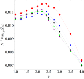
Figure 5: Quantites entering Eq.(39) for lattices with different $\displaystyle N$. In particular, $\displaystyle N=100$ (red full circles), $\displaystyle N=400$ (blue squares), $\displaystyle N=900$ (black diamonds), $\displaystyle N=1600$ (green triangles), $\displaystyle N=2500$ (purple reversed triangles).

Figure 6: Quantites entering Eq.(39) for lattices with different $\displaystyle N$. In particular, $\displaystyle N=100$ (red full circles),$\displaystyle N=400$ (blue squares), $\displaystyle N=900$ (black diamonds), $\displaystyle N=1600$ (green triangles), $\displaystyle N=2500$ (purple reversed triangles).

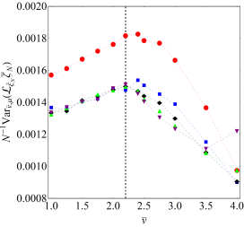
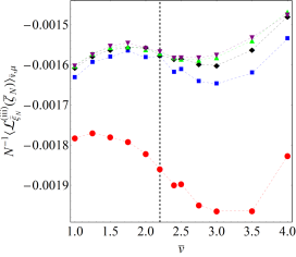
Figure 7: Quantites entering Eq.(39) for lattices with different $\displaystyle N$. In particular, $\displaystyle N=100$ (red full circles),$\displaystyle N=400$ (blue squares), $\displaystyle N=900$ (black diamonds), $\displaystyle N=1600$ (green triangles), $\displaystyle N=2500$ (purple reversed triangles).

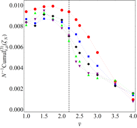
Figure 8: Quantites entering Eq.(39) for lattices with different $\displaystyle N$. Left panel: third cumulant of $\displaystyle\overline{\zeta}_{N}$ for $\displaystyle N=100$ (red full circles), $\displaystyle N=400$ (blue squares), $\displaystyle N=900$ (black diamonds), $\displaystyle N=1600$ (green triangles), $\displaystyle N=2500$ (purple reversed triangles). Right panel: fourth cumulant of $\displaystyle\overline{\zeta}_{N}$ computed at the transition energy density $\displaystyle\bar{v}_{c}\simeq 2.2$, here a systematic deviation from the gaussian scaling with $\displaystyle N$ is well evident.

The results of numerical simulations are reported for each single single term entering Eq.(39). When properly rescaled with $\displaystyle N$, under the hypothesis of diffeomorphism (at any $\displaystyle N$ and also asymptotically) of the equipotential hypersurfaces, all these terms are expected to be uniformly bounded with $\displaystyle N$. Very interestingly, it is found that across the vertical dashed line denoting the phase transition point at the potential energy density $\displaystyle\bar{v}_{c}\simeq 2.2$ all these terms do not show any tendency to change with $\displaystyle N$, except for the case $\displaystyle N=10\times 10$ (for which $\displaystyle 36\%$ of the total number of sites belong to the boundary, making the finite size effects more relevant). There is only one very significative exception, the fourth cumulant of $\displaystyle\overline{\zeta}_{N}$ which, computed around the transition value, is found to systematically grow with $\displaystyle N$. This has been computed by means of the relation

$$\mathrm{Cuml}^{(4)}_{N\bar{v},\mu}\overline{\zeta}=\frac{d}{dv}\left[\mathrm{Cuml}^{(3)}_{N\bar{v},\mu}\overline{\zeta}_{N}\right]-3\left\langle\overline{\zeta}_{N}\right\rangle_{\overline{v},\mu}\left(\mathrm{Corr}_{\overline{v},\mu}\left(\Delta\overline{\zeta}_{N};\mathcal{L}_{\overline{\boldsymbol{\boldsymbol{\xi}}}_{N}}(\overline{\zeta}_{N})\right)\right)$$ (61)

where the derivative of the third cumulant is evaluated numerically.

This means that $\displaystyle\overline{\zeta}_{N}$ is not a Gaussian random process along a MCMC the invariant measure of which is the microcanonical measure. As $\displaystyle\overline{\zeta}_{N}$ is proved to be a Gaussian random process under the constraining hypothesis of asymptotic diffeomorphicity of the level sets $\displaystyle\{\Sigma_{N\bar{v}}^{V_{N}}\}_{\bar{v}\in[\bar{v}_{0},\bar{v}_{1}]}$, the growth with $\displaystyle N$ of $\displaystyle N^{-1}\mathrm{Cuml}^{(4)}_{N\bar{v},\mu}\overline{\zeta}$ entails the loss of asymptotic diffeomorphicity among the $\displaystyle\{\Sigma_{N\bar{v}}^{V_{N}}\}_{\bar{v}<\bar{v}_{c}}$ and the $\displaystyle\{\Sigma_{N\bar{v}}^{V_{N}}\}_{\bar{v}>\bar{v}_{c}}$ for some $\displaystyle\bar{v}_{c}$. This means that the 2D lattice $\displaystyle\phi^{4}$ model does not fulfil a basic requirement of the Main theorem formulated in the present work. Therefore, the 2D lattice $\displaystyle\phi^{4}$ model is not a counterexample to the present version of the topological necessity theorem.

As it has been pointed out in Remark 3, a second order phase transition in the microcanonical ensemble is associated with an asymptotic discontinuity of the third derivative of the entropy and hence an asymptotic divergence of the fourth derivative of the entropy

V Historical overview and challenges of the topological theory of phase transitions

After the investigation of specific, exactly solvable models fernando ; exact1 ; exact2 ; exact3 ; exact4 corroborating the Topological Hypothesis, during the last decade and a half other systems have been studied, shedding doubts on the general validity of the new theory. Even if all these studies are important to better define the validity limits of the Topological Hypothesis, some authors have too quickly drawn fatal verdicts against it.

In fact, for the sake of clarity, let us begin by remarking that the proposed theory applies a-priori to systems described by smooth, finite-range potentials such that the level sets $\displaystyle\Sigma_{v}^{V_{N}}$ and their associated balls $\displaystyle M_{v}^{V_{N}}$ qualify as good differentiable and compact manifolds. Moreover, as we have preliminarily discussed in Ref.vaff , and as it is thoroughly tackled throughout the present paper, topology changes - as loss of diffeomorphicity among differentiable manifolds - can take place also in the absence of critical points of the potential function.

Thus, coming to specific examples, in kastner-cazz the author tackled a system modelling in one-dimension a localization-delocalization transition of interfaces. This so-called Burkhardt model was also considered in romani1d where the pinning potential was considered in a modified version. The absence of coincidence between topological and thermodynamical transitions was reported in both Refs. kastner-cazz and romani1d .

However, the Burkhardt model has two bad properties with respect to the conditions of the Topological Hypothesis, formalized by the theorems in Refs.book ; prl1 ; NPB1 ; NPB2 and by the theorem proved in the present paper. In fact, the pinning potentials considered in Refs. kastner-cazz and romani1d are singular as they need infinitely steep potential barriers to constrain the coordinates of the system on a semi-infinite positive line, and the configuration-space submanifolds are noncompact.

In grinza , and also in romani1d , another one dimensional model was considered, the so-called Peyrard–Bishop model describing DNA denaturation. In Ref. romani1d the authors considered also a modified version of the Peyrard–Bishop model, and for both versions of the model the topological transition is found at a critical value of the potential energy which does not correspond to critical energy value of the thermodynamic transition. The configuration space submanifolds corresponding to these models are noncompact, and the critical manifolds - containing only one critical point of infinite coordinates - are infinitely large. Again, these models are outside the domain of validity of the theorems in Refs.book ; prl1 ; NPB1 ; NPB2 and in the present paper.

Another model, allegedly disproving the topological theory, is the mean-field Berlin–Kac spherical model. In Ref. stariolo the two cases of zero and non-zero external field were considered. In the former case there is a continuous phase transition and in the latter case there is no phase transition. The two cases did not display much difference when considered from the topological viewpoint. However, for this model there is a strong statistical ensemble inequivalence, in fact the continuous phase transition for zero external field is only predicted in the framework of canonical ensemble, whereas it is absent in the framework of microcanonical ensemble kastnerRT ; kastner-ineq which is the reference framework where the topological theory is formulated. Thus there is no contradiction. Moreover, considering that the ergodic invariant measure of Hamiltonian flows is the microcanonical measure, and considering that the objective reality of any physical system is dynamics, the microcanonical ensemble has to be considered the fundamental statistical ensemble.

By the way, this is not the only case of this kind of ensemble inequivalence, for example, though working in the opposite way, the clustering phase transition in a self-gravitating $\displaystyle N$-body system found in the microcanonical ensemble framework is completely absent in the canonical ensemble mnras .

In stariolo1 the authors tackle a modified version of the Berlin-Kac model which is constrained with the introduction of a long-range correlation among the degrees of freedom. In spite of the claim that this model is the first case of short-range, confining potential where the phase transition is not entailed by a topology change in phase space or configuration space, the spherical constraint, by limiting the freedom of mutual independent variation of all the degrees of freedom, makes this model a long-range interaction one. And even though the spherical constraint is, so to speak, a weak constraint, It plays a crucial role because without it the model is trivial.

Another system apparently going against the topological theory is the mean-field $\displaystyle\phi^{4}$ model. The phase transition point of this model does not correspond to the presence of critical points of the potential, that is, it has no topological counterpart romani ; schilling ; baroni . Some correspondence between the topological and thermodynamic transitions was recovered for this model in Ref. romani by introducing a suitable weakening of the Topological Hypothesis. However, the mean-field $\displaystyle\phi^{4}$ model undergoes a $\displaystyle{\mathbb{Z}}_{2}$-symmetry-breaking phase transition, as in the case of the short range $\displaystyle\phi^{4}$ model vaff . As a consequence, the reason why this system is not a counterexample of the topological theory is twofold: on the one side it violates the condition of asymptotic diffeomorphicity of the level sets $\displaystyle\Sigma_{v}^{V_{N}}$ put forward in the present work, and, on the other side, in the broken symmetry phase even in the absence of critical points of the potential in the $\displaystyle N\to\infty$ limit the splitting of the configuration space into two disjoint submanifolds is actually a major change of topology in correspondence with the phase transition point.

All the attempts at falsifying the Topological Hypothesis are useful to better outline the domain of validity of the theory, which, on the other hand, is not intended to apply to all the possible phase transitions. The theory can leave outside its validity domain models with unbound and long-range potentials without being invalidated by this kind of systems.

Summarizing, the Topological Hypothesis is coherent and now free of counterexamples, nevertheless the above mentioned alleged counterexamples have the merit of showing that some - perhaps much - work remains to be done, mainly in the case of long-range interactions. In fact, for example, for the exactly solvable model in Refs.exact2 ; exact3 , which is a mean-field XY model, thus with long-range interactions, a sharp topological transition in configuration space is clearly at the origin of the phase transition. At variance with the mean-field $\displaystyle\phi^{4}$ model described by polynomial potentials, the mean-field XY model is described by a potential bounded from above. Whether and why this fact could explain the different conformity of these models to the topological description of their transitional behaviour is still a wide open question.

VI Concluding remarks

The present work is a substantial leap forward of the topological theory of phase transitions which was seriously undermined by the counterexample mentioned in the previous sections. The theory is rooted in the study of thermodynamical phase transitions from the viewpoint of microscopic Hamiltonian dynamics. As Hamiltonian flows can be identified with geodesics flows of suitable differentiable manifolds, it turned out that across a phase transition point these manifolds undergo major geometrical changes of topological origin. This is to remark that topology is, so to speak, naturally implied by the fundamental/dynamical approach and it is not just conjectured to play a role. The first important consequence of this approach is that the occurrence of a phase transition is not the consequence of a loss of analyticity of statistical measures but it is already encoded in the potential function describing the interactions among the degrees of freedom of a system. This makes the thermodynamic limit dogma no longer necessary neither from the conceptual side nor from the mathematical description side. And, of course, this is interesting when tackling phase transition phenomena in mesoscopic and nanoscopic systems. Moreover, phase transitions phenomena in the absence of symmetry-breaking - and thus in the absence of an order parameter - have been successfully tackled in the topological framework, at present, at least in the case of a model with a gauge symmetry dualising , for a 2D-model with an $\displaystyle O(2)$ symmetry undergoing a Kosterlitz-Thouless transition kosterlitz , and for the protein folding transition proteinfold . It is worth mentioning that in a recent paper loris - partly based on some results given in gori2022 - a purely geometric theory of phase transitions has been put forward. In this work it is proposed that Bachmann’s classification of phase transitions bachmann ; PRL-Bachmann for finite-size systems can be reformulated in terms of geometric properties of the energy level sets associated to a given Hamiltonian function; here the energy-derivatives of the entropy are associated to specific combinations of geometric curvature properties of the energy level sets. There is no contradiction between the geometric theory and the topological theory of phase transitions, mainly because sharp changes of the geometry of the leaves (energy level sets) of a foliation of phase space can be generically attributed to deeper changes of topological kind. However, the precise relationship between geometry and topology is given by theorems in differential topology and, unfortunately, there is only a few number of these theorems that can be constructively used (essentially the Gauss-Bonnet-Hopf, the Chern-Lashof, and Pinkall theorems book ). Therefore the geometric approach has some practical advantage with the respect to the topological one in what curvature properties of the energy level sets can be always explicitly computed.

It is noteworthy that, in principle, the topological approach to classical phase transitions - addressed in the present work, as well as the geometric approach in Ref.loris - can be extended to the treatment of quantum transitions by means of Wick’s analytic prolongation to imaginary times of the path-integral generating functional of quantum field theory, this allows to map a quantum system onto a formally classical one described by a classical partition function written with the euclidean Lagrangian action, on lattice to have a countable number of degrees of freedom book .

Finally, recent developments of powerful computational methods in algebraic topology, like those of persistent homology Carlsson ; noi , provide the topological description of phase transitions with new useful constructive tools in addition to the existing concepts and methods of differential topology.

Appendix A. Uniform boundedness of $\displaystyle{\mathscr{R}}$

Let us now show how asymptotic diffeomorphicity entails uniform boundedness with $\displaystyle N$ of the Ricci scalar curvature defined in equation (17), and using $\displaystyle\|\boldsymbol{\xi}\|=\|\nabla V(\textit{{q}})\|^{-1}$,

$${\mathscr{R}}=\frac{1}{N(N-1)}\left\{-\triangle\log\|\boldsymbol{\xi}\|^{-1}+\nabla\cdot\left[\triangle V(\textit{{q}})\ \boldsymbol{\xi}\right]\right\}\ ,$$ (62)

where the second term in the r.h.s. is

$$\displaystyle\nabla\cdot\left[\triangle V(\textit{{q}})\ \boldsymbol{\xi}\right] \displaystyle= \displaystyle[\nabla\triangle V(\textit{{q}})]\cdot\boldsymbol{\xi}+[\triangle V(\textit{{q}})]\nabla\cdot\boldsymbol{\xi}$$ (63)

$$\displaystyle= \displaystyle\triangle V(\textit{{q}})\ \partial^{i}\left(\frac{\partial_{i}V(\textit{{q}})}{\|\nabla V(\textit{{q})}\|^{2}}\right)+\frac{\partial_{j}V(\textit{{q})}}{\|\nabla V(\textit{{q})}\|^{2}}\partial^{j}\partial^{k}\partial_{k}V(\textit{{q}})$$ (64)

and using convenzione

$$\displaystyle\triangle V(\textit{{q}}) \displaystyle= \displaystyle\nabla\cdot[\nabla V(\textit{{q}})]=\nabla\cdot[\|\nabla V(\textit{{q}})\|^{2}\boldsymbol{\xi}]=\partial^{i}\left(\frac{\xi_{i}}{\|\boldsymbol{\xi}\|^{2}}\right)$$ (65)

$$\displaystyle= \displaystyle\frac{1}{\|\boldsymbol{\xi}\|^{2}}(\partial^{i}\xi_{i})-\frac{4}{\|\boldsymbol{\xi}\|^{2}}\frac{\xi_{i}}{\|\boldsymbol{\xi}\|}\frac{\xi^{j}}{\|\boldsymbol{\xi}\|}(\partial^{i}\xi_{j})$$ (66)

after Eqs.(6),(7), (8) all these terms are uniformly bounded in $\displaystyle N$, and so does $\displaystyle\nabla\cdot\boldsymbol{\xi}$, moreover, the denominator $\displaystyle\|\boldsymbol{\xi}\|^{-4}\sim N^{2}$ is compensated by the pre-factor $\displaystyle 1/N(N-1)$. therefore the second term in the r.h.s. of Eq.(63) is also uniformly bounded in $\displaystyle N$. Then the first term of Eq.(63) is obtained by applying the operator $\displaystyle\boldsymbol{\xi}\cdot\nabla$ to Eq.(66), and, after trivial algebra of the same kind of that leading to Eq.(66), one obtains a lengthy expression - containing mixed second order derivatives of the components of $\displaystyle\boldsymbol{\xi}$ - which are uniformly bounded under the assumption of asymptotic diffeomorphicity. On the other hand, for smooth and regularized potentials, if $\displaystyle n$ is the coordination number of the potential, and $\displaystyle{\textgoth m}_{0}$ is the maximum value of $\displaystyle\partial^{i}\partial_{i}V$, then $\displaystyle\triangle V(\textit{{q}})$ is bounded by $\displaystyle n\,{\textgoth m}_{0}N/[N(N-1)]$. By the same token, if $\displaystyle{\textgoth m}_{1}$ is the maximum value of $\displaystyle\partial_{j}\partial^{i}\partial_{i}V$ then $\displaystyle\boldsymbol{\xi}\cdot\nabla\triangle V(\textit{{q}})$ is uniformly bounded by $\displaystyle n\,{\textgoth m}_{1}B$, where $\displaystyle B$ is the constant of Eq.(8).

Now, coming to the first term in the r.h.s. of Eq.(62), that is $\displaystyle\partial^{i}\left(\partial_{i}\log\|\nabla V(\textit{{q}})\|\right)$, we have

$$\displaystyle\partial^{i}\left(\partial_{i}\log\|\boldsymbol{\xi}\|^{-1}\right) \displaystyle= \displaystyle\partial^{i}(\|\boldsymbol{\xi}\|\partial_{i}\|\boldsymbol{\xi}\|^{-1})=\partial^{i}\|\boldsymbol{\xi}\|\partial_{i}\|\boldsymbol{\xi}\|^{-1}+\|\boldsymbol{\xi}\|\ \partial^{i}\partial_{i}\|\boldsymbol{\xi}\|^{-1}$$ (67)

$$\displaystyle= \displaystyle-\frac{1}{\|\boldsymbol{\xi}\|^{2}}(\partial_{i}\|\boldsymbol{\xi}\|)^{2}+\left[-\frac{1}{\|\boldsymbol{\xi}\|}(\partial^{i}\partial_{i}\|\boldsymbol{\xi}\|)+\frac{2}{\|\boldsymbol{\xi}\|^{2}}(\partial_{i}\|\boldsymbol{\xi}\|)^{2}\right]$$ (68)

$$\displaystyle= \displaystyle-\frac{1}{\|\boldsymbol{\xi}\|}(\partial^{i}\partial_{i}\|\boldsymbol{\xi}\|)+\frac{1}{\|\boldsymbol{\xi}\|^{2}}(\partial_{i}\|\boldsymbol{\xi}\|)^{2}$$ (69)

and

$$\frac{1}{\|\boldsymbol{\xi}\|^{2}}(\partial_{i}\|\boldsymbol{\xi}\|)^{2}=\frac{1}{\|\boldsymbol{\xi}\|^{2}}(\partial_{i}\sqrt{\xi_{j}\xi^{j}})^{2}=\frac{\xi_{j}\xi^{j}}{\|\boldsymbol{\xi}\|^{4}}(\partial_{i}\xi_{j})^{2}$$ (70)

which is uniformly bounded after Eqs.(6),(7),(8) and the pre-factor $\displaystyle 1/N(N-1)$. Then for the first term in Eq.(69) we get

$$\frac{1}{\|\boldsymbol{\xi}\|}(\partial^{i}\partial_{i}\|\boldsymbol{\xi}\|)=\frac{1}{\|\boldsymbol{\xi}\|}\partial^{i}\left(\frac{\xi^{j}}{\|\boldsymbol{\xi}\|}\,\partial_{i}\xi_{j}\right)=\frac{1}{\|\boldsymbol{\xi}\|}\left[\frac{\xi^{j}}{\|\boldsymbol{\xi}\|}\,\partial^{i}\partial_{i}\xi_{j}+\frac{(\partial_{i}\xi_{j})^{2}}{\|\boldsymbol{\xi}\|}-\frac{\xi_{j}\xi^{j}\,(\partial_{i}\xi_{j})^{2}}{\|\boldsymbol{\xi}\|^{3}}\right]$$ (71)

which, under the same conditions mentioned above, is also uniformly bounded in $\displaystyle N$. The relevant consequence is that under the assumption of asymptotic diffeomorphicity of potential energy level sets, the scalar Ricci curvature $\displaystyle{\mathscr{R}}$ in Eq.(62) is uniformly bounded in $\displaystyle N$ and so do all the principal curvatures of the manifolds transformed under the action of the vector field $\displaystyle\boldsymbol{\xi}$.

Appendix B. Lie derivatives of the vector field $\displaystyle\boldsymbol{\xi}$

In the following we derive explicit expressions of the Lie derivatives of the one-parameter diffeomorphism-generating vector field $\displaystyle\boldsymbol{\xi}$ for a potential $\displaystyle V$ in ”critical points-free” regions of configuration space $\displaystyle(\mathcal{X},g_{\mathbb{R}^{N}}$ endowed with a Riemannian metric. Let $\displaystyle(q_{1},....,q_{N})$ be a set of coordinates in configuration space. In what follows we shall refer to $\displaystyle\partial_{i}=\partial/\partial q^{i}$ so that $\displaystyle(\nabla V)_{i}=\partial_{i}V$ and the Hessian $\displaystyle(\mathrm{Hess}V)_{ij}=\partial^{2}_{ij}V$.
With these chioces the divergence of the vector field $\displaystyle\zeta=\mathrm{div}_{\mathbb{R}^{N}}\boldsymbol{\xi}$ reads:

$$\mathrm{div}_{\mathbb{R}^{N}}\boldsymbol{\xi}=\dfrac{\Delta V}{\|\nabla V\|^{2}}-2\dfrac{\nabla V\cdot(\mathrm{Hess}V\nabla V)}{\|\nabla V\|^{4}}$$ (72)

where $\displaystyle\Delta(\cdot)=\sum_{i}^{N}\partial^{i}\partial_{i}(\cdot)$ is the Laplacian operator in the Euclidean configuration space and $\displaystyle\|\boldsymbol{X}\|^{2}=g_{\mathbb{R}^{N}}(\boldsymbol{X},\boldsymbol{X})$ is the Euclidean norm. As the Lie derivative operator along the flow generated by the vector field $\displaystyle\boldsymbol{\xi}$ is

$$\mathcal{L}_{\boldsymbol{\xi}}(\cdot)=(\boldsymbol{\xi}\cdot\nabla)(\cdot)=\sum_{i=1}^{N}\dfrac{\partial^{i}V}{\|\nabla V\|^{2}}\partial_{i}(\cdot)$$ (73)

the first derivative reads

$$\begin{split}\mathcal{L}_{\boldsymbol{\xi}}(\zeta)=&\dfrac{\nabla V\cdot\nabla(\Delta V)}{\|\nabla V\|^{4}}-2\dfrac{(\nabla V\cdot\mathrm{Hess}(V)\nabla V)\Delta V+2\|\mathrm{Hess}V\nabla V\|^{2}+\mathrm{D}^{3}V(\nabla V,\nabla V,\nabla V)}{\|\nabla V\|^{6}}+\\ &+8\dfrac{(\nabla V\cdot\mathrm{Hess}V\nabla V)^{2}}{\|\nabla V\|^{8}}\end{split}$$ (74)

where $\displaystyle\mathrm{D}^{3}V(\nabla V,\nabla V,\nabla V)=\partial^{3}_{ijk}V\partial_{i}V\partial_{j}V\partial_{k}V$.

The second order derivative (with the aid of symbolic manipulation with Mathematica) reads

$$\displaystyle\mathcal{L}_{\boldsymbol{\xi}}^{(ii)}(\zeta)=\dfrac{\nabla(\Delta V)\cdot(\mathrm{Hess}V\nabla V)+\nabla V\cdot(\mathrm{Hess}(\Delta V)\nabla V)}{\|\nabla V\|^{6}}+$$ (75)

$$\displaystyle- \displaystyle 2\Biggr{[}\dfrac{\Delta V\mathrm{D}^{3}V(\nabla V,\nabla V,\nabla V)+2\Delta V\|\mathrm{Hess}V\nabla V\|^{2}+4(\mathrm{Hess}V\nabla V)\cdot(\mathrm{Hess}V\mathrm{Hess}V\nabla V)}{\|\nabla V\|^{8}}+$$

$$\displaystyle+ \displaystyle\dfrac{7\mathrm{D}^{3}V(\mathrm{Hess}V\nabla V,\nabla V,\nabla V)+\mathrm{D}^{4}V(\nabla V,\nabla V,\nabla V,\nabla V)+3(\nabla V\cdot\mathrm{Hess}V\nabla V)(\nabla V\cdot\nabla(\Delta V))}{\|\nabla V\|^{8}}\Biggr{]}+$$

$$\displaystyle+ \displaystyle\dfrac{28(\nabla V\mathrm{Hess}V\nabla V)\left[2\|\mathrm{Hess}V\nabla V\|^{2}+\mathrm{D}^{3}V(\nabla V,\nabla V,\nabla V)\right]+12(\nabla V\mathrm{Hess}V\nabla V)^{2}\Delta V}{\|\nabla V\|^{10}}+$$

$$\displaystyle- \displaystyle 64\dfrac{(\nabla V\mathrm{Hess}V\nabla V)^{3}}{\|\nabla V\|^{12}}$$

and the third order derivative (with the aid of symbolic manipulation with Mathematica) reads

$$\begin{split}&\mathcal{L}_{\boldsymbol{\xi}}^{(iii)}(\zeta)=\dfrac{3\nabla V\cdot\mathrm{Hess}(\Delta V)\mathrm{Hess}V\nabla V+\mathrm{D}^{3}\Delta V(\nabla V,\nabla V,\nabla V)+\mathrm{D}^{3}V(\nabla V,\nabla V,\nabla(\Delta V))}{\|\nabla V\|^{8}}+\\ &+\dfrac{\nabla(\Delta V)\cdot\mathrm{Hess}V\mathrm{Hess}V\nabla V}{\|\nabla V\|^{8}}-2\Biggr{[}\dfrac{4\mathrm{D}^{3}V(\nabla V,\nabla V,\nabla V)(\nabla V\cdot\nabla(\Delta V))}{\|\nabla V\|^{10}}+\\ &+\dfrac{7\mathrm{D}^{4}V(\nabla V,\nabla V,\nabla V,\mathrm{Hess}V\nabla V)}{\|\nabla V\|^{10}}+\\ &+\dfrac{15\mathrm{D}^{3}V(\nabla V,\nabla V,\mathrm{Hess}V\mathrm{Hess}V\nabla V)+7\|\mathrm{D}^{3}V(\nabla V,\nabla V)\|^{2}+18\mathrm{D}^{3}V(\mathrm{Hess}V\nabla V,\mathrm{Hess}V\nabla V,\nabla V)}{\|\nabla V\|^{10}}+\\ &+\dfrac{4\mathrm{D}V(\nabla V,\nabla V,\nabla V,\mathrm{Hess}V\nabla V)+\mathrm{D}^{5}V(\nabla V,\nabla V,\nabla V,\nabla V,\nabla V)+8(\nabla V\cdot\nabla(\Delta V))\|\mathrm{Hess}V\nabla V\|^{2}}{\|\nabla V\|^{10}}+\\ &+\dfrac{8\|\mathrm{Hess}V\mathrm{Hess}V\nabla V\|^{2}+7\mathrm{D}^{3}V(\nabla V,\nabla V,\mathrm{Hess}V\nabla V)\Delta V}{\|\nabla V\|^{10}}+\\ &\dfrac{\Delta V\mathrm{D}^{4}V(\nabla V,\nabla V,\nabla V,\nabla V)+4\Delta V(\mathrm{Hess}V\nabla V)\cdot\mathrm{Hess}V\mathrm{Hess}V\nabla V}{\|\nabla V\|^{10}}+\\ &+\dfrac{6(\mathrm{Hess}V\cdot\mathrm{Hess}V\nabla V)(\nabla V\cdot\mathrm{Hess}(\Delta V)\nabla V)+6(\mathrm{Hess}V\cdot\mathrm{Hess}V\nabla V)(\nabla(\Delta V)\cdot\mathrm{Hess}V\nabla V)}{\|\nabla V\|^{10}}\Biggr{]}+\\ &+4\Biggr{[}\dfrac{7\left(\mathrm{D}^{3}V(\nabla V,\nabla V,\nabla V)\right)^{2}+28\mathrm{D}^{3}V(\nabla V,\nabla V,\nabla V)\|\mathrm{Hess}V\nabla V\|^{2}}{\|\nabla V\|^{12}}+\\ &+\dfrac{10\Delta V\mathrm{D}^{3}V(\nabla V,\nabla V,\nabla V)(\nabla V\cdot\mathrm{Hess}V\nabla V)}{\|\nabla V\|^{12}}+\\ &+\dfrac{28\|\mathrm{Hess}V\nabla V\|^{4}+20\Delta V\|\mathrm{Hess}V\nabla V\|^{2}(\nabla V\cdot\mathrm{Hess}V\nabla V)}{\|\nabla V\|^{12}}+\\ &+\dfrac{(\nabla V\cdot\mathrm{Hess}V\nabla V)[77\mathrm{D}^{3}V(\nabla V,\nabla V,\mathrm{Hess}V\nabla V)}{\|\nabla V\|^{12}}+\\ &+\dfrac{11\mathrm{D}^{4}V(\nabla V,\nabla V,\nabla V,\nabla V)+44(\mathrm{Hess}V\nabla V)\cdot(\mathrm{Hess}V\mathrm{Hess}V\nabla V)}{\|\nabla V\|^{12}}+\\ &+\dfrac{15(\mathrm{Hess}V\cdot\mathrm{Hess}V\nabla V)(\nabla V\cdot\nabla(\Delta V))]}{\|\nabla V\|^{12}}\Biggr{]}+\\ &-8\Biggr{[}\dfrac{59\mathrm{D}^{3}V(\nabla V,\nabla V,\nabla V)(\nabla V\cdot\mathrm{Hess}V\nabla V)^{2}}{\|\nabla V\|^{14}}+\\ &+\dfrac{(\nabla V\cdot\mathrm{Hess}V\nabla V)^{2}[118\|\mathrm{Hess}V\nabla V\|^{2}+15\Delta V(\nabla V\cdot\mathrm{Hess}V\nabla V)]}{\|\nabla V\|^{14}}\Biggr{]}+768\dfrac{(\nabla V\cdot\mathrm{Hess}V\nabla V)^{4}}{\|\nabla V\|^{16}}\end{split}$$ (76)

VII Acknowledgments

This work has been done within the framework of the project MOLINT which has received funding from the Excellence Initiative of Aix-Marseille University - A*Midex, a French “Investissements d’Avenir” programme. This work was also partially supported by the European Union’s Horizon 2020 Research and Innovation Programme under grant agreement no. 964203 (FET-Open LINkS project). Roberto Franzosi acknowledges support by the QuantERA ERA-NET Co-fund 731473 (Project Q-CLOCKS) and the support by the National Group of Mathematical Physics (GNFM-INdAM). Matteo Gori thanks the financial support of DARPA (USA) for his long term visit at Howard University at Washington D.C. during which part of this work was done.

References

• (1) C.N. Yang, and T.D. Lee, Statistical theory of equations of state and phase transitions I. Theory of condensation, Phys. Rev. 87, 404 - 409 (1952); T.D. Lee, and C.N. Yang, Statistical theory of equations of state and phase transitions II. Lattice gas and Ising model, Phys. Rev. 87, 410 - 419 (1952).
• (2) A comprehensive account of the Dobrushin-Lanford-Ruelle theory and of its developments can be found in: H.O. Georgii, Gibbs Measures and Phase Transitions, Second Edition, (De Gruyter, Berlin 2011).
• (3) D.H.E. Gross, Microcanonical Thermodynamics. Phase Transitions in “Small” Systems, (World Scientific, Singapore, 2001).
• (4) M. Bachmann, Thermodynamics and Statistical Mechanics of Macromolecular Systems, (Cambridge University Press, New York, 2014).
• (5) K. Qi and M. Bachmann, Classification of Phase Transitions by Microcanonical Inflection-Point Analysis, Phys. Rev. Lett. 120,180601 (2018).
• (6) M. Pettini, Geometry and Topology in Hamiltonian Dynamics and Statistical Mechanics, IAM Series n.33, (Springer, New York, 2007).
• (7) M. Pettini, Geometrical hints for a nonperturbative approach to Hamiltonian dynamics, Phys. Rev. E47, 828 (1993).
• (8) G. Carlsson, J. Gorham, M. Kahle, and J. Mason, Computational topology for configuration spaces of hard disks, Phys. Rev. E85, 011303 (2012).
• (9) Y. Baryshnikov, P. Bubenik, and M. Kahle, Min-type Morse theory for configuration spaces of hard spheres, Int. Math. Res. Notices, doi:10.1093/imrn/rnt012, (2013).
• (10) O. B. Eriçok, K. Ganesan, and J. K. Mason, Configuration spaces of hard spheres, arXiv:2106.10315v3 [cond-mat.stat-mech]
• (11) D.C. Brody, D.W. Hook, and L. P. Hughston, Quantum phase transitions without thermodynamic limits, Proc. Roy. Soc. A (London) 463, 2021 (2007).
• (12) P. Buonsante, R. Franzosi, A. Smerzi, Phase transitions at high energy vindicate negative microcanonical temperature, arXiv:1506.01933.
• (13) G.E. Volovik, Quantum phase transitions from topology in momentum space, in Quantum analogues : from phase transitions to black holes and cosmology, p.31-73 (Springer, Berlin Heidelberg, 2007).
• (14) L. Angelani, R. Di Leonardo, G. Parisi, and G. Ruocco, Topological description of the aging dynamics in simple glasses, Phys. Rev. Lett. 87, 055502 (2001).
• (15) P.G. Debenedetti, and F. H. Stillinger, Supercooled liquids and the glass transition, Nature 410, 259 (2001) .
• (16) S. Risau-Gusman, A.C. Ribeiro-Teixeira, and D.A. Stariolo, Topology, phase transitions, and the spherical model, Phys. Rev. Lett. 95, 145702 (2005).
• (17) F.A.N. Santos, L.C.B. da Silva, and M.D. Coutinho-Filho, Topological approach to microcanonical thermodynamics and phase transition of interacting classical spins, Journal of Statistical Mechanics: Theory and Experiment 2017, 013202 (2017).
• (18) D.A. Garanin, , R. Schilling, and A. Scala, Saddle index properties, singular topology, and its relation to thermodynamic singularities for a $\displaystyle\phi^{4}$ mean-field model, Phys. Rev. E70, 036125 (2004).
• (19) David Cimasoni, and Robin Delabays, The topological hypothesis for discrete spin models, J.Stat.Mech., 033216 (2019).
• (20) P. Grinza, and A. Mossa, Topological origin of the phase transition in a model of DNA denaturation, Phys. Rev. Lett. 92, 158102 (2004).
• (21) O.M. Becker, and M. Karplus, The topology of multidimensional potential energy surfaces: theory and application to peptide structure and kinetics, J. Chem. Phys. 106, 1495 (1997).
• (22) L. Caiani, L. Casetti, C. Clementi, and M. Pettini, Geometry of Dynamics, Lyapunov Exponents, and Phase Transitions, Phys. Rev. Lett. 79, 4361 (1997).
• (23) L. Caiani and L. Casetti and C. Clementi and G. Pettini and M. Pettini and R. Gatto, Geometry of dynamics and phase transitions in classical lattice $\displaystyle\phi^{4}$ theories, Phys.Rev. E57, 3886 (1998).
• (24) C.L. Brooks, J. N. Onuchic, and D. J. Wales. ”Taking a walk on a landscape.” Science 293, 612-613 (2001).
• (25) D.J. Wales, ”A microscopic basis for the global appearance of energy landscapes.” Science 293, 2067-2070 (2001).
• (26) Fernando A. N. Santos, Ernesto P. Raposo, Maurício D. Coutinho-Filho, Mauro Copelli, Cornelis J. Stam, Linda Douw, Topological phase transitions in functional brain networks, https://www.biorxiv.org/content/10.1101/469478v3
• (27) L.Casetti, M. Pettini, E.G.D. Cohen, Geometric approach to Hamiltonian dynamics and statistical mechanics, Phys. Rep. 337, 237-342 (2000), and references quoted therein.
• (28) R. Franzosi, and M. Pettini, Theorem on the origin of Phase Transitions, Phys. Rev. Lett. 92, 060601 (2004).Ä
• (29) R. Franzosi, M. Pettini, and L. Spinelli, Topology and Phase Transitions I. Preliminary results, Nucl. Phys. B782 [PM], 189 (2007).
• (30) R. Franzosi and M. Pettini, Topology and Phase Transitions II. Theorem on a necessary relation, Nucl. Phys. B782 [PM], 219 (2007).
• (31) M. Kastner and D. Mehta, Phase Transitions Detached from Stationary Points of the Energy Landscape, Phys. Rev. Lett. 107, 160602 (2011).
• (32) M. Gori, R. Franzosi and M. Pettini, Topological origin of phase transitions in the absence of critical points of the energy landscape, J. Stat. Mech. 093204 (2018).
• (33) M.W. Hirsch, Differential Topology, (Springer, New York 1976).
• (34) J.A. Thorpe, Elementary Topics in Differential Geometry, (Springer-Verlag, New York 1979), p. 55.
• (35) Y. Zhou, A Simple Formula for Scalar Curvature of Level Sets in Euclidean Spaces, arXiv:1301.2202 [math.DG].
• (36) Christina Sormani, How Riemannian Manifolds Converge, In: Dai X., Rong X. (eds) Metric and Differential Geometry. Progress in Mathematics, vol 297. Birkhäuser, Basel (2012).
• (37) R.S. Palais and C. Terng, Critical Point Theory and Submanifold Geometry, (Springer, New York 1988).
• (38) H.  Federer, Geometric measure theory (Springer, Berlin, 1969).
• (39) P. Laurence, On the convexity of geometric functional of level for solutions of certain elliptic partial differential equations, ZAMP 40, 258 (1989).
• (40) P. Brémaud, Markov Chains, (Springer, New York 2001), Chapter 7.
• (41) See Lemma 3.1 in: J. Alvarez-Vizoso, M. Kirby, and C. Peterson, Integral invariants from covariance analysis of embedded Riemannian manifolds, arxiv.org/abs/1804.10425v1
• (42) A.I. Khinchin, Mathematical Foundations of Statistical Mechanics, (Dover Publications, Inc., New York 1949).
• (43) Consider a family of random variables $\displaystyle\{X_{k}\}$, if $\displaystyle X_{i}$ and $\displaystyle X_{j}$ satisfy finite-range dependence, i.e. there is a positive integer $\displaystyle n_{0}$ such that if $\displaystyle|i-j|>n_{0}$ then $\displaystyle X_{i}$ and $\displaystyle X_{j}$ are independent. A law of large numbers for $\displaystyle X_{i}$ can then be easily proved.
• (44) L. Caiani, L. Casetti, and M. Pettini, Hamiltonian dynamics of the two-dimensional lattice $\displaystyle\phi^{4}$ model, J. Phys.A: Math.Gen. 31, 3357 (1998).
• (45) L. Casetti, E.G.D. Cohen, and M. Pettini, Topological origin of the phase transition in a mean-field model, Phys. Rev. Lett. 82, 4160 (1999).
• (46) L. Casetti, E.G.D. Cohen, and M. Pettini, Exact result on topology and phase transitions at any finite $\displaystyle N$, Phys. Rev. E 65, 036112 (2002).
• (47) L. Casetti, M. Pettini and E.G.D. Cohen, Phase transitions and topology changes in configuration space, J. Stat. Phys. 111, 1091 (2003).
• (48) L. Angelani, L. Casetti, M. Pettini, G. Ruocco, and F. Zamponi, Topology and Phase Transitions: from an exactly solvable model to a relation between topology and thermodynamics, Phys. Rev. E71, 036152 (2005).
• (49) M. Kastner, Unattainability of a purely topological criterion for the existence of a phase transition for nonconfining potentials, Phys. Rev. Lett.93, 150601 (2004).
• (50) L. Angelani, G. Ruocco, and F. Zamponi, Relationship between phase transitions and topological changes in one-dimensional models, Phys. Rev. E72, 016122 (2005).
• (51) A.C. Ribeiro Teixeira, and D.A. Stariolo, Topological hypothesis on phase transitions: The simplest case, Phys. Rev. E70, 016113 (2004).
• (52) M. Kastner, and O. Schnetz, On the mean-field spherical model, J. Stat. Phys.122, 1195 (2006).
• (53) M. Kastner, Topological approach to phase transitions and inequivalence of statistical ensembles, Physica A359, 447 (2006).
• (54) M. Cerruti-Sola, P. Cipriani and M. Pettini, On the clustering phase transition in self-gravitating N-body systems, Monthly Not. Roy. Astron. Soc. 328, 339 (2001).
• (55) S. Risau-Gusman, A.C. Ribeiro Teixeira, and D.A. Stariolo, Topology, phase transitions, and the spherical model, Phys. Rev. Lett.95, 145702 (2005).
• (56) A. Andronico, L. Angelani, G. Ruocco, and F. Zamponi, Topological properties of the mean-field $\displaystyle\phi^{4}$ model, Phys. Rev. E70, 041101 (2004).
• (57) F. Baroni, Phase Transitions and Topological Changes in Configuration Space for Mean-Field Models, Laurea Thesis in Physics (University of Florence, 2002).
• (58) G. Pettini, M. Gori, R. Franzosi, C. Clementi, and M. Pettini, On the origin of phase transitions in the absence of symmetry-breaking, Physica A516, 376 (2018).
• (59) Gh. Bel-Hadj-Aissa, M. Gori, R. Franzosi, and M. Pettini, Geometrical and Topological study of the Kosterlitz-Thouless Phase Transition in the XY model in two dimensions, J. Stat. Mech., 023206 (2021).
• (60) L. Di Cairano, R. Capelli, G. Bel-Hadj-Aissa, and M. Pettini, Topological origin of protein folding transition, https://hal.archives-ouvertes.fr/hal-03504864 .
• (61) L. Di Cairano, The geometric theory of phase transitions, J. Phys. A: Math. Theor. 55, 27LT01 (2022).
• (62) M. Gori, Configurational microcanonical statistical mechanics from Riemannian geometry of equipotenital level sets, https://arxiv.org/abs/2205.14536
• (63) G. Carlsson and A. Zomorodian, Persistent homology - a survey, Discrete Comput. Geom. 33, 249 (2005); G. Carlsson, Topology and data, Bull. Am. Math. Soc. 2, 255 (2009).
• (64) I. Donato, M. Gori, M. Pettini, G. Petri, S. De Nigris, R. Franzosi, and F. Vaccarino Persistent Homology analysis of Phase Transitions, Phys. Rev. E93, 052138 (2016); and references therein for persistent homology.