Embedding Recycling for Language Models

Abstract

Real-world applications of neural language models often involve running many different models over the same corpus. The resulting high computational cost has led to interest in techniques that can reuse the contextualized embeddings produced in previous runs to speed training and inference of future ones. We refer to this approach as embedding recycling (ER). While multiple ER techniques have been proposed, their practical effectiveness is still unknown because existing evaluations consider very few models and do not adequately account for overhead costs. We perform an extensive evaluation of ER across eight different models (17 to 900 million parameters) and fourteen tasks in English. We show how a simple ER technique that caches activations from an intermediate layer of a pretrained model, and learns task-specific adapters on the later layers, is broadly effective. For the best-performing baseline in our experiments (DeBERTa-v2 XL), adding a precomputed cache results in a >90% speedup during training and 87-91% speedup for inference, with negligible impact on accuracy. Our analysis reveals important areas of future work, and we release code and documentation for our experiments at https://github.com/allenai/embeddingrecycling.

1 Introduction

Large pretrained language models form the foundation of modern NLP, and continue to push the state-of-the-art on a wide range of natural language processing tasks (Devlin et al., 2019; Liu et al., 2019b; Bommasani et al., 2021). Larger models tend to offer superior accuracies (Kaplan et al., 2020), but also entail higher computational costs. The steep computational cost associated with large neural language models slows down experimentation, increases financial barriers to the technology, and contributes to global climate change (Strubell et al., 2019; Dodge et al., 2022).

Our work studies how to reduce computational cost for workloads in which many distinct models are run over the same text. For example, a scholarly search tool that helps users find and understand relevant literature may run separate models for entity recognition, topic classification, relation extraction, summarization, question answering, and so on over a large corpus of papers. New and improved models for the tasks are developed frequently, necessitating additional runs. The need for repeated model runs has also been noted for other applications in previous work, including news applications Du et al. (2020) and virtual assistants Wei et al. (2022). Further, repeated runs also occur very frequently during model development, when exploring model variants or executing multiple training epochs.

Recent work has introduced ways to reduce computational cost in such settings by re-using model activations from one task to speed up other ones Du et al. (2020); Wei et al. (2022). A pretrained language model’s internal activations form a contextualized embedding, which reflects syntactic and semantic knowledge about the input text (Goldberg, 2019; Wiedemann et al., 2019; Rogers et al., 2020) which can be useful across a variety of downstream tasks. We define embedding recycling (ER) as the technique of caching certain activations from a previous model run, and re-using them to improve the efficiency of future training and inference. Recycling imposes a small computation time cost the first time a model processes a text, in order to compute and populate the cache. Thereafter, all subsequent runs on the text can use the precomputed cache, improving efficiency.

While previous work has shown the promise of ER approaches, the existing evaluations are limited. For example, Du et al. (2020) and Wei et al. (2022) each evaluate ER for only one or two base models. Likewise, for ER techniques that cache activations on persistent storage, the storage and time cost of the cache itself has yet to be quantified. In this paper, we present a more comprehensive evaluation of ER with several models and tasks, along with a thorough efficiency analysis. We study a simple layer-recycling ER method that caches the activations from an intermediate layer of a pretrained model, and uses those cached activations as the starting point when the same input sequence is seen again during fine-tuning or inference. We show that even this simple method yields substantial improvements to throughput at small or no cost to accuracy on average. Our results provide the strongest evidence to date that ER can be a practically important technique for reducing costs for NLP systems, but as we discuss in section 6, they also suggest important challenges that must be addressed in future work.

Our contributions are summarized below:

• We propose embedding recycling as a method for lowering the computational costs of training and inference for language models, and explore layer recycling with two techniques: standard fine-tuning and parameter-efficient adapters.

• Our experiments with eight models across a wide range of tasks show that layer recycling is generally effective. For the best-performing ER model on our tasks- DeBERTa-XL with adapters, we find that layer recycling nearly matches performance of the original model while providing a 87-91% speedup at inference time, and greater than 90% speedup at training time.

• We explore open challenges for embedding recycling and present questions for future work.

2 Related Work

The embedding recycling technique we investigate is based on findings from prior work suggesting that not all layers of a pretrained transformer are equally important for end-task finetuning. Shallower layers tend to converge earlier in training than deeper layers (Raghu et al., 2017; Morcos et al., 2018), and weights of later layers change more than earlier ones (Kovaleva et al., 2019), suggesting that earlier layers tend to extract universal features whereas later layers focus on task-specific modeling. Lee et al. (2019) find that 90% of fully fine-tuned performance can be reached when fine-tuning only the final quarter of a transformer’s layers and leaving the rest frozen.

Several proposed methods vary the number of frozen layers over the course of training, approaching or exceeding the performance of fully fine-tuned models while substantially speeding up the training process (Raghu et al., 2017; Xiao et al., 2019; Brock et al., 2017). Similar to our approach, some dynamic freezing methods also employed caching mechanisms (Liu et al., 2021; He et al., 2021), but the dynamic number of frozen layers means the cache applies only at training time and only for a single task. In contrast, we cache embeddings from the pretrained model, which can then be reused across multiple downstream tasks and applied at inference time as well.

Other recent studies have sought to improve model inference speed by skipping computations in later layers. Sajjad et al. (2020) found that in some cases up to half of the layers can be removed from the model with only a 1-3% drop in task performance. Early exit strategies have also been proposed, which allow the model to dynamically decide when to skip later layers (Cambazoglu et al., 2010; Xin et al., 2020). SkipBERT (Wang et al., 2022) combined early exiting with an approach in which cached n-gram embeddings approximate the intermediate activations of new inputs. Lester et al. (2021) explored prompt-tuning as a parameter-efficient approach for adapting frozen language models without adjusting model weights, conditioning language models with soft prompts to perform downstream tasks.

Precomputing text representations to speed up future processing on the same data is commonly done when creating fixed-size document-level embeddings for use on document-level tasks (Conneau et al., 2017; Cohan et al., 2020); in contrast, we study contextualized token-level embeddings that can be used for tasks such as named entity recognition (NER) and question answering. ReadOnce Transformers (Lin et al., 2021) do consider multi-task variable-length document representations, but do so in a setting where a cached document representation is paired with a query text (such as a question or prompt); the approach is pretrained with QA data and evaluated on QA and summarization, rather than tasks such as text classification or NER where the entire input can be cached.

Du et al. (2020) propose an approach similar to ours that caches general-purpose token-level model representations, trained in a multi-task setting; however, that approach only applies a small MLP to the stored representations and reports a meaningful drop in accuracy (greater than 2% on average) compared to fully fine-tuned models. We find that reusing the later layer parameters of a pretrained transformer in addition to the cached activations often enables us to essentially match fully fine-tuned model accuracy while reducing computational cost.

Wei et al. (2022) combine layer freezing and knowledge distillation to create a multi-task model. They do not consider caching activations on persistent storage as we do, but instead re-use activations across tasks at inference time via a branching multi-task model. They use a two stage process where $12-N$ layers are fine-tuned for each individual task keeping $N$ frozen layers. This is followed by distillation of the $N$ layers for further computational gains. We take advantage of the parameter efficient adapter modules (Houlsby et al., 2019), and replace this process with a single step of fine-tuning a frozen base model that has adapters attached only to the deeper layers.

Our work also has connections to work on memory- and retrieval-augmented language modeling. Prior work on using memory (e.g., Grave et al. (2016); Dai et al. (2019); Rae and Razavi (2020); Wu et al. (2022)) generally focuses on modeling long-range context and caching representations of older history in a sequence, while work on retrieval (e.g., Guu et al. (2020); Karpukhin et al. (2020)) focuses on fetching text from a knowledge base or corpus to serve as additional context. In both cases, the aim is to use representations of additional text (from earlier in a document or from a knowledge base) to improve modeling of new inputs. In contrast, our work focuses on caching the representations of an entire sequence to speed up computation for new tasks.

3 Methods

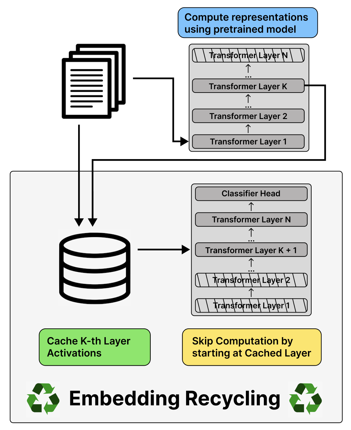
Figure 1: Overview of the embedding recycling approach. In the figure, the K-th layer activations are saved for future fine-tuning on downstream tasks, skipping redundant computations of earlier layers in the transformer model.

In the transformer architecture (Vaswani et al., 2017), an input sequence $x$ of length $S$ and dimension $d$ is transformed with a function $F:\mathbb{R}^{S\times d}\rightarrow\mathbb{R}^{S\times d}$ defined by the composition of $N$ transformer layers $F^{(1)},...,F^{(N)}$ as follows:

$$\texttt{F}^{\ell}(x)=\texttt{LN}(\texttt{FF}^{\ell}(\;x^{\prime})+x^{\prime})$$ (1)

$$\texttt{x'}=\texttt{LN}\Big{(}\texttt{MH}^{\ell}(x)+x\Big{)}$$ (2)

where LN is a layer normalization (Ba et al., 2016), FF is a feed forward network, and MH is the self-attention layer that consists of multiple heads and contextualizes the input sequence vector. The output of each layer is used as input to the next layer.

$$h^{\ell+1}=F^{\ell}(h^{\ell})$$ (3)

Our approach is to cache the output representations $h^{k}\in\mathbb{R}^{S\times d}$ at a certain layer $k$ and reuse them for fine-tuning on a new given task. We refer to this process of caching and reusing the output representations of a layer as layer recycling. This enables us to reduce the size of the transformer model from $N$ layers to $N-k$ layers, reducing the computational cost during fine-tuning and inference.

Note that the key requirement of layer recycling is that we first need to process the entire data with the transformer model and cache the representations, so that we could later reuse these representations many times during fine-tuning and inference on new tasks. We experiment with two types of layer recycling approaches as explained next.

We start with a pretrained transformer $F$ (e.g., BERT) consisting of $F^{(1)},...,F^{(k)},...,F^{(N)}$ layers. During the first epoch of fine-tuning for any given task, we run the transformer over a corpus $\mathcal{C}$ and cache the output representations of layer $k$ for each instance $c$ in $\mathcal{C}$, i.e., $h^{k}_{c\in\mathcal{C}}$. However, for every subsequent epoch of fine-tuning using the same transformer model, we only run and fine-tune the latter $N-k$ layers $F^{(k+1)},...,F^{(N)}$. We can either train all of the weights in the layers (which we refer to as reduced models), or only train adapter modules added on the layers (discussed below). In either case, for the instance $c$ in the dataset $\mathcal{C}$ we simply retrieve and use the previously cached representation $h^{k}_{c\in\mathcal{C}}$ as input to layer $F^{(k+1)}$. This avoids the extra computation through layers $F^{(1)},...,F^{(k)}$ but adds a small cost for retrieving the representation from storage (see subsection 5.4 for efficiency analysis).

3.1 Adapters

We evaluate whether combining recycling with Adapter modules (Houlsby et al., 2019) can improve performance over fully fine-tuned models. Adapters are typically used to improve the parameter efficiency of fine-tuning and mitigate the storage costs of large language models. They also enable more sample-efficient fine-tuning and can result in improved fine-tuning performance (Karimi Mahabadi et al., 2022).

Adapter modules contain a down-projection, an up-projection, and a residual connection module: $h\leftarrow h+(f(h\mathbf{W}_{down})\mathbf{W}_{up})$. The adapters are separately inserted after the MH and the FF layers in the transformer architecture (Equation 2). Further, Rücklé et al. (2021) experiment with dropping adapters from the lower transformer layers to provide inference time speedup. In our experiments, adapters are added to the latter half of transformer layers in the reduced transformer models. As in standard layer recycling, the pretrained original transformer $F$ first caches the intermediate activations $h^{k}_{c\in\mathcal{C}}$ for each input in a selected corpus at layer $k$. Then the first $k$ layers are removed from the transformer. During fine-tuning, the cached representations are fed as input to the later $N-k$ layers of the transformer, which consist of the frozen transformer layers plus trainable adapter parameters. Thus, we fine-tune only the additional 6-8% parameters introduced by the adapters. We refer to learning adapters on all layers as the full adapter setting and the layer recycling version as the reduced adapter setting.

4 Experimental Setup

We now present our experiments evaluating whether recycled embeddings can be paired with reduced large language models to maintain accuracy while improving training and inference speed. We explore the effectiveness of embedding recycling across a variety of different tasks, datasets, and transformer models.

4.1 Models

Our full-size models include the encoder transformers BERT, SciBERT (Beltagy et al., 2019), RoBERTa (Liu et al., 2019b), and DeBERTa (He et al., 2020). We also experiment with the encoder-decoder T5 model (Raffel et al., 2019). We selected these architectures since they are widely-used pretrained transformers across a variety of tasks in different domains. We experiment with multiple sizes of these models, including distilled (Sanh et al., 2019; Wang et al., 2020, 2021), base, and large variants, to gauge the effectiveness of recycled embeddings with an increase in the network size.

To investigate the effectiveness of layer recycling, we test several reduced models in which we use caching to reduce 50% of the layers (e.g., caching layer 12 in RoBERTa-large and layer 6 in BERT-base). We compare each reduced model to its fully fine-tuned counterpart across the text classification, NER, and QA tasks. The hardware details and hyperparameters for our models are specified in Appendix A.

4.2 Datasets

For our experiments, we focus on three core NLP tasks: text classification, named-entity recognition (NER), and extractive question-answering (QA). Scientific papers, due to their immutable nature, are an especially appropriate target for embedding recycling, so we focus much of our evaluation on the scientific domain. For text classification, we selected Chemprot (Kringelum et al., 2016), SciCite (Cohan et al., 2019), and SciERC (Luan et al., 2018). For NER, we used BC5CDR (Li et al., 2016), JNLPBA (Collier and Kim, 2004), and NCBI-Disease (Doğan et al., 2014). For QA, we chose the TriviaQA (Joshi et al., 2017) and SQuAD (Rajpurkar et al., 2016) datasets.

5 Results

5.1 Standard Fine-tuning

	RoBERTa Large		(Sci)BERT		DeBERTa V2 XL		T5 Large		MiniLM L6-H768		MiniLM L6-H384		DistilBERT
Task	Rdc	Full	Rdc	Full	Rdc	Full	Rdc	Full	Rdc	Full	Rdc	Full	Rdc	Full
ChemProt	84.3	83.9	84.0	84.0	86.8	86.7	84.6	84.1	78.3	79.3	76.9	74.6	80.3	79.1
SciCite	85.0	85.5	86.6	86.0	85.2	84.4	86.3	84.9	84.5	84.6	83.7	82.8	84.1	84.0
SciERC-Rel	80.2	80.4	76.7	79.8	79.9	80.2	77.4	80.2	74.8	78.2	72.1	68.9	74.9	72.9
[1pt/1pt] Classification Avg.	83.2	83.3	82.4	83.3	84.0	83.8	82.8	83.1	79.2	80.7	77.6	75.4	79.8	78.7
bc5cdr	90.0	90.4	90.7	91.3	91.3	91.8	90.7	89.9	87.8	87.5	85.9	88.3	88.3	88.7
JNLPBA	79.4	78.7	78.8	79.0	78.5	78.2	79.6	80.0	77.3	76.9	74.0	77.2	78.6	78.5
NCBI-disease	93.0	93.2	93.4	92.9	93.3	93.4	92.8	93.5	91.1	92.1	89.9	91.7	90.5	91.3
[1pt/1pt] NER Avg.	87.5	87.4	87.7	87.7	87.7	87.8	87.7	87.8	85.4	85.5	83.3	85.7	85.8	86.2
TriviaQA	78.2	79.8	67.4	69.1	80.6	81.8	77.4	78.2	72.2	73.8	69.2	71.0	64.7	66.8
SQuAD	91.8	93.6	87.5	88.5	94.5	94.6	93.7	93.9	85.0	87.0	89.0	89.6	84.8	85.4
[1pt/1pt] QA Avg.	85.0	86.7	77.5	78.8	87.5	88.2	85.5	85.9	78.6	80.4	79.1	80.3	74.8	76.1

Table 1: Test scores of reduced (Rdc) models on the text classification, NER, and QA tasks. Bold indicates the best average F-1 score between the reduced and fully fine-tuned (Full) versions of each model over 10 runs. For the ChemProt dataset, we report the micro F-1 scores instead, following past work (Beltagy et al., 2019). The reduced BERT-sized models generally offer similar performance to their full counterparts (scoring within 0.2% when averaged across RoBERTa and SciBERT for the six tasks), and substantially outperform the distilled models.

The results for standard fine-tuning of either full or reduced models are shown in Table 1. For the text classification and NER tasks, the reduced BERT-sized and larger models perform similarly to their fine-tuned counterparts on average, and substantially outperform the distilled models. The reduced distilled models also perform well on those tasks compared to the distilled originals, on average, although there is more variance across models and tasks compared to BERT-sized models. We validate our fully fine-tuned baselines by comparing our results with prior work (Beltagy et al., 2019), finding that our scores land within 1.33% on average and typically score above the previous baselines.

For QA tasks, we found that fully fine-tuning works somewhat better than reduced configurations across all the explored models (Table 1). Generally, reduced configurations typically lag by 1 to 2 points in F-1 score. One possible hypothesis is that the QA datasets are generally much larger than the datasets we used for other tasks (100k-150k examples vs 4k-20k examples for text classification and NER); however, in additional experiments we found that subsampling the QA training sets to 5% of their original size only increased the gap, suggesting that dataset size does not explain the failure of reduced models on this task. We also validate our fully fine-tuned baselines for QA tasks by comparing our results with Yasunaga et al. (2022), finding that our scores differ by less than half a point on average.

Finally, we explored using lightweight multi-layer perceptrons (MLPs) as classifier heads, given their success in prior work. While Du et al. (2020) paired multi-task encoders with 2-layer MLPs, we paired frozen pretrained transformer models with 2-layer MLPs and found that they underperformed trainable layers dramatically, by 26% on average across the classification and NER tasks.

5.2 Adapters

	RoBERTa Large			(Sci)BERT			DeBERTa V2 XL			T5 Large
Task	Rdc + Half Adpt	Full Adpt	Full	Rdc + Half Adpt	Full Adpt	Full	Rdc + Half Adpt	Full Adpt	Full	Rdc + Half Adpt	Full Adpt	Full
ChemProt	84.1	85.2	83.9	84.2	84.9	84.0	87.2	86.5	86.7	84.3	84.9	84.1
SciCite	82.4	82.9	85.5	85.5	84.6	86.0	84.6	85.0	84.4	85.3	84.5	84.9
SciERC-Rel	85.7	85.9	80.4	86.0	85.5	79.8	82.9	82.1	80.2	76.2	75.6	80.2
[1pt/1pt] Classification Avg.	84.1	84.7	83.3	85.2	85.0	83.3	84.9	84.6	83.8	81.9	81.7	83.1
bc5cdr	90.0	90.6	90.4	90.0	90.9	91.3	90.7	91.1	91.8	79.9	85.7	89.9
JNLPBA	79.1	79.2	78.7	79.8	78.3	79.0	79.3	79.0	78.2	78.8	79.5	80.0
NCBI-disease	92.8	93.1	93.2	93.1	93.0	92.9	93.3	93.5	93.4	92.1	92.5	93.5
[1pt/1pt] NER Avg.	87.3	87.6	87.4	87.6	87.4	87.7	87.8	87.9	87.8	83.6	85.9	87.8
TriviaQA	78.5	79.8	79.8	67.4	68.9	69.1	81.6	82.3	81.8	77.0	77.5	78.2
SQuAD	93.5	93.4	93.6	87.9	87.9	88.5	94.7	93.9	94.6	90.6	91.0	93.9
[1pt/1pt] QA Avg.	86.0	86.6	86.7	77.6	78.4	78.8	88.1	88.1	88.2	83.8	84.3	85.9

Table 2: Test scores of reduced adapter (Rdc + Half Adpt) models on the text classification, NER, and QA tasks. Bold indicates the best average F-1 score between the reduced adapter, full adapter (Full Adpt), and fully fine-tuned (Full) versions of each model over 10 runs. For the ChemProt dataset, we report the micro F-1 scores instead, following past work (Beltagy et al., 2019). The reduced, adapter-based transformer models offer similar performance to their full counterparts (scoring within 0.4% when averaged across RoBERTa, SciBERT, and DeBERTa for the eight tasks), and substantially outperform the distilled models.

Our results for reduced adapter models are shown in Table 2. We see that in general, for all the models except for T5-Large, the adapter-based approaches are superior to standard fine-tuning on our tasks. Further, layer recycling remains effective with adapters. Compared to the full adapter baseline, the reduced adapters for RoBERTa-Large, BERT, SciBERT, and DeBERTa models only show a 0.19% reduction in accuracy. Additionally, compared to the fully fine-tuned baseline, these reduced adapters models have a 0.19-0.23% reduction in accuracy. Likewise, in contrast to the full fine-tuning results above, QA accuracy for the top-performing DeBERTa adapter model remains unchanged on average after layer recycling, with the reduced adapter model performing better on one QA task and worse on the other.

5.3 GLUE Results

GLUE task	DeBERTa V2 XL
	Rdc + Half Adpt	Full Adpt	Rdc	Full
CoLA	70.9	71.3	70.8	71.2
SST-2	96.9	97.1	97.1	97.4
[1pt/1pt] Single Sentence Avg.	83.9	84.2	84.0	84.3
MRPC	93.9	94.0	93.4	93.9
STS-B	92.4	92.7	92.5	92.8
[1pt/1pt] Similarity and Paraphrase Avg.	93.2	93.4	93.0	93.4
MNLI-m	91.7	92.0	91.0	91.4
QNLI	95.0	95.1	94.1	94.8
[1pt/1pt] NLI Avg.	93.3	93.6	92.6	93.1

Table 3: Test scores of reduced (Rdc) and reduced adapter (Rdc + Half Adpt) models on GLUE for DeBERTa V2 XL. Bold indicates the best average score between the reduced and fully fine-tuned (Full) versions for the standard and adapter-based configurations. Each score is averaged over 5 runs. We report the scores using the standard GLUE metric for each corresponding task.

For our best-performing model DeBERTa v2 XL, we also provide further experiments on datasets from the GLUE benchmark (Wang et al., 2018), to allow easier comparison against speedup techniques from previous work. We present results on the CoLA, SST-2, MRPC, STS-B, MNLI, and QNLI tasks from GLUE. For our experiments, we tried both our standard reduced models and our reduced adapter models. We found that embedding recycling was successful across the GLUE tasks, with an average accuracy drop of 0.3 points in return for a significant increase in both training and inference time as outlined in Table 5 and Table 4. We note that due to the high computational cost of these experiments, we take existing hyperparameter settings from previous work that worked well for the full models, and also use these for reduced models. Further hyperparameter optimization of the reduced models might improve performance.

5.4 Efficiency Analysis

	Inference Time (Speedup over Baseline)
Model	Baseline	Recycling		Avg. F1 diff when recycling
		FP32 cache	FP16 cache
NVIDIA A10G
MiniLM L6-H384	183 ms	154 ms (+21%)	123 ms (+67%)	$-0.2$
MiniLM L6-H768	325 ms	201 ms (+56%)	195 ms (+66%)	$-0.4$
BERT Base	647 ms	351 ms (+84%)	343 ms (+88%)	$-0.3$
BERT Large	1943 ms	1066 ms (+86%)	1004 ms (+93%)	$-0.2$
DeBERTa V2-XLarge	1914 ms	1010 ms (+89%)	985 ms (+94%)	$-0.1$
NVIDIA A6000
MiniLM L6-H384	123 ms	105 ms (+18%)	100 ms (+23%)	$-0.2$
MiniLM L6-H768	208 ms	161 ms (+29%)	150 ms (+38%)	$-0.4$
BERT Base	416 ms	269 ms (+55%)	245 ms (+59%)	$-0.3$
BERT Large	1235 ms	662 ms (+86%)	643 ms (+92%)	$-0.2$
DeBERTa V2-XLarge	1430 ms	777 ms (+84%)	758 ms (+89%)	$-0.1$

Table 4: Average inference runtime comparison (in ms/batch, averaged over 7 runs) between vanilla encoders and models that cache embeddings on disk. For all runs, cache the middle layer of the encoder. We assume the cache is already precomputed when calculating timings; thus, maximum speedup is 100%. Overall, the larger the model, the higher the speedup from re-using representations. Further, accelerators with fewer execution units (A10G) benefit more from recycling embeddings. Finally, using half precision for embeddings improves speed up across the board, while halving storage size.

To estimate the real-world benefit of recycling embeddings for different tasks, we provide a minimal PyTorch implementation of embedding recycling. This implementation and the following results correspond to both the standard layer recycling approach and the adapter-based layer recycling approach since they follow parallel processes for gradient descent during training and computations during inference, despite the additional 6-8% of parameters added by the trainable adapters. To show that training times do not differ substantially, we also measured the training time the transformer models take to converge to their optimal weights. We found both approaches take approximately the same time to complete training (Table 16).

We evaluated the impact of recycling embeddings on four different architectures and two different hardware platforms. For models, we considered two efficient transformer models (MiniLMv2 (Wang et al., 2020, 2021) models with $l=6$ layers and embeddings of size $h=384$ and $h=768$), two medium sized models ($\text{BERT}_{\textsc{Base}}$, $l=12$, $h=768$; $\text{BERT}_{\textsc{Large}}$, $l=24$, $h=1024$), and a large model ($\text{DeBERTa}_{\textsc{V2-XLarge}}$, $l=24$, $h=1536$). We evaluated embeddings on a efficiency-oriented AI accelerator (NVIDIA A10G), as well as on a high-performance GPU (NVIDIA A6000).

We controlled for differences among tasks considered in tables Table 1, 2, and 3, such as length of sequences and number of samples, by simulating a sequence classification task on Qasper (Dasigi et al., 2021), which includes the full-text of over a thousand academic manuscripts. We run all models with a fixed batch size of 128. For all models, we reduce exactly half of their layers by recycling, which results in a maximum theoretical speed-up of 100%. A run over the corpus consists of 335 batches, and we average results over seven runs.

Table 4 shows the results of caching embeddings to recycle on disk. Overall, we found that all models benefit from embedding recycling, achieving an average speedup ranging from 18 to 86%. Unsurprisingly, larger models benefit more from recycling than smaller ones; this is due to the fact that loading embeddings cached on disk adds a small latency penalty to a model run, which is more noticeable in the case of smaller models. For example, we achieve an 84% speedup when running $\text{BERT}_{\textsc{Base}}$ with embedding recycling on an A10G GPU, which is roughly equivalent to the latency of a $\text{MiniLM}_{\text{L6-H768}}$ model without recycling (351 vs 325 ms per batch on average); this result would us allow to run more accurate models while maintaining the efficiency of shallower architectures.

Model	Training (ms/batch, amortized over 6 epochs)				Speedup
	No Recycling (NR)	Model Frozen (F)	Saving + Recycling (SR)	Only Recycling (R)	NR vs SR	F vs SR	NR vs R
NVIDIA A10G
$\text{MiniLM}_{384}$	51 $\pm$ 1	30 $\pm$ 1	32 $\pm$ 6	25 $\pm$ 4	+59%	-7%	+104%
$\text{MiniLM}_{768}$	90 $\pm$ 4	56 $\pm$ 1	50 $\pm$ 4	45 $\pm$ 3	+80%	+12%	+100%
$\text{BERT}_{\textsc{Base}}$	173 $\pm$ 2	112 $\pm$ 1	90 $\pm$ 4	87 $\pm$ 3	+92%	+24%	+99%
$\text{BERT}_{\textsc{Large}}$	347 $\pm$ 1	246 $\pm$ 1	181 $\pm$ 2	176 $\pm$ 2	+92%	+36%	+97%
$\text{DeBERTa}_{\textsc{XLarge}}$	380 $\pm$ 2	286 $\pm$ 1	199 $\pm$ 1	194 $\pm$ 1	+91%	+44%	+96%
NVIDIA A6000
$\text{MiniLM}_{384}$	41 $\pm$ 1	24 $\pm$ 1	26 $\pm$ 5	22 $\pm$ 3	+55%	-8%	+81%
$\text{MiniLM}_{768}$	61 $\pm$ 1	38 $\pm$ 1	40 $\pm$ 5	34 $\pm$ 3	+52%	-5%	+82%
$\text{BERT}_{\textsc{Base}}$	117 $\pm$ 1	78 $\pm$ 1	60 $\pm$ 3	58 $\pm$ 2	+94%	+30%	+102%
$\text{BERT}_{\textsc{Large}}$	326 $\pm$ 2	212 $\pm$ 1	167 $\pm$ 2	161 $\pm$ 1	+96%	+26%	+103%
$\text{DeBERTa}_{\textsc{XLarge}}$	359 $\pm$ 2	250 $\pm$ 1	184 $\pm$ 1	178 $\pm$ 1	+95%	+35%	+102%

Table 5: Average training runtime comparison (in ms per batch, $\pm$ stdev over 7 runs) between vanilla encoders and models that cache embeddings on disk. For all runs, we cache the middle layer of the encoder; thus, theoretical speedup is 100%. Time per batch is amortized over 6 epochs ($2,000$ steps), the lowest number to convergence over all datasets (c.r.f. Table 16). We present results in four settings: no recycling (NR), freezing ½ of the layers during training (F), 1 training epoch during which embeddings are saved to disk followed by 5 epochs where recycling is enabled (SR), and 6 epochs where embeddings are already saved (R). Overall, we found that embedding recycling speeds up training even when embeddings need to be cached to disk during the first pass. Compared to freezing, saving and recycling improves training time for all but MiniLM models (F vs SR).

Table 4 also includes results when storing embeddings using half precision (that is, cache embeddings in FP16 rather FP32). The smaller embeddings lead to improvements for all models and hardware, ranging from $+8\%$ to $+46\%$. Further, it has no impact on performance, as it changes predicted scores by at most $10^{-3}$ across all tasks evaluated in this work.

We also note that less capable hardware benefits more from caching embeddings. For example, $\text{BERT}_{\textsc{Base}}$ achieves a speedup of $84\%$ on an A10G GPU, while on A6000, the speedup is a more modest $55\%$. This is an expected result: fewer and slower execution cores/accelerator memory impact overall model latency. Further, we note that, despite the smaller relative gains, the more powerful GPU is always faster in absolute terms compared with the less capable one.

It is important to note that these gaps from maximum achievable speedup are only observed when performing inference; for training, we observe almost perfect speed-up for all models and hardware configurations except for the smaller MiniLM models. For example, $\text{BERT}_{\textsc{Base}}$ requires $17.38\pm 1.32\text{ ms/batch}$ without recycling, compared to $8.67\pm 2.18\text{ ms/batch}$ when recycling. Even when considering the additional time to cache embeddings to disk during the first pass, embedding recycling still achieves close to optimum speedup on all models except MiniLMs, where its gains hover between 52% and 82% (“NR vs SR” column in Table 5). When training for just 6 epochs (or roughly $2,000$ steps), recycling embeddings is faster than simply freezing half of the parameters for all models but MiniLM (“F vs SR” column in Table 5); this is due to the relatively higher cost of caching layers to disk in case of smaller models. In these cases, we empirically found that recycling achieves faster training time than freezing after 12 epochs or $4,000$ training steps; since smaller models typically require more epochs to converge, we conclude that recycling is generally preferable to partially freezing a model during training. For $\text{BERT}_{\textsc{Base}}$ and larger models, embedding recycling is also more efficient than layer freezing, providing a $+20\%$ to $+45\%$ speed-up after just 6 training epochs.

We also benchmarked the storage requirements of recycling embeddings. For a sequence of 512 tokens and a hidden model dimension of 768, caching embeddings requires 1.6 MB with 32-bit precision or 0.8 MB with 16-bit precision. This translates to 15.5 MB per paper in Qasper (papers are, on average 4,884 WordPiece tokens long). Weighing the storage cost and compute savings of ER, we find that it is cost-effective in cloud environments only if the corpus is reprocessed several times per month, but is cost-effective on local hardware even with infrequent (yearly) corpus reprocessing (details in subsection A.8 of the appendix).

6 Discussion and Future Work

Our experiments raise several questions and suggest multiple avenues for future work, including:

• Our layer recycling strategy is a straightforward ER approach, but previous work has suggested that weighted pooling across layers can perform better compared to any single layer in many cases (Liu et al., 2019a; Du et al., 2020). Recycling pooled activations may offer improved results. What is the best way to capture and store the syntactic and semantic knowledge encoded in the activations of a model for later recycling?

• As noted in the previous section, naive storage methods for ER can be cost-prohibitive in some settings, and finding ways to mitigate this cost (e.g., by compressing the stored activations) will be important for making ER broadly applicable.

• Our experiments show that the right recycling approach may be task-specific and model-specific. For example, with standard fine-tuning as shown in Table 8, caching layer 12 in RoBERTa-large is most effective for NER and text classification, whereas it is not effective for QA (but layer 6 performs much better). Which embeddings to retrieve and recycle for a task, and the right architecture (e.g. number of layers) to use when consuming the recycled embeddings, represents a large decision space. Methods that can help practitioners automatically choose among public or private shared embedding sets and associated model designs, given their task and objectives for accuracy and computational cost, may be important to make ER an effective practical tool.

• We present results with encoder-only and encoder-decoder models, on classification tasks. Determining whether the approach is effective for generative tasks and autoregressive models is an important question for future work.

• While we show that ER can be effective when coupled with distillation, whether other techniques like quantization and early exiting remain effective in combination with ER is an open question.

• We focus on the setting where the exact same text, at the length of a full document, is being reused for multiple tasks. In practice, we may often perform a task on text that is similar to but not exactly the same as one for which we have cached embeddings (e.g., a Wikipedia page that has been revised). Further, even a completely new document will have similarities and overlapped spans with previously processed ones. Studying ER in these settings, e.g. through a combination of layer recycling and the SkipBERT approach which can apply to unseen passages via cached n-grams (Wang et al., 2022), is an area of future work.

• Finally, it is possible to explore cross-model embedding recycling. We attempted a straightforward implementation of such approach by using recycling embeddings from a larger model into a smaller consumer model. However, the results did not show improvements (Appx. A.3). Developing and evaluating new approaches for this setting is an important item for future work.

7 Conclusion

We have presented embedding recycling, a general technique for reusing previous activations of neural language models to improve the efficiency of future training and inference. We show how a simple technique of caching a layer of activations in a pretrained model is effective. We validate our approach in experiments across fourteen tasks and eight model architectures. We find that recycling typically has small or no impacts to accuracy on average, but does yield substantial throughput increases demonstrated through a careful efficiency analysis. We also discuss several open challenges for future work.

8 Limitations

As discussed in detail in our future work section, several advances are important to make embedding recycling a broadly applicable practical technique. In addition, the techniques we evaluate primarily benefit transformer language models run on GPU-based architectures with rapid storage, components which are not available to all NLP researchers and practitioners. Our experiments demonstrate positive results with one representative embedding recycling technique, but do not directly evaluate all recycling variants proposed earlier in the literature. Finally, the datasets used in our experiments were in English, a high-resource language with robust pretrained models which may benefit embedding recycling. Future work should expand on the applicability of embedding recycling by using non-English datasets in lower-resource settings to determine the breadth of its applicability.

Appendix A Experimental Setup and Additional Results

A.1 Fine-tuning Transformer Models

The candidate transformer models are fine-tuned using configurations suggested by Devlin et al. (2019), Ding et al. (2022) and Houlsby et al. (2019). For text classification, we feed the final hidden state of the [CLS] token into a linear classification layer. For NER and QA, we feed the final hidden states of each token into a linear classification layer with a softmax output.

For all of the models, we apply a dropout of 0.1 to the transformer outputs and optimize for cross entropy loss using Adam (Kingma and Ba, 2015). We employ a batch size of 32 across all tasks. We fine-tune using early stopping with a patience of 10, using a validation set for calculating loss for each epoch. We use a linear warmup followed by linear decay for training (Howard and Ruder, 2018), testing the following learning rate options: 1e-3, 2e-3, 1e-4, 2e-4, 1e-5, 2e-5, 5e-5, and 5e-6. For the text classification and NER datasets, we select the best performing learning rate for each transformer model on the development set and report the corresponding test results. For the QA datasets, we select the best performing learning rate for each transformer model on the training set and report the corresponding results on the validation set. Additionally, for the adapter modules used in certain model configurations, we test bottleneck dimensions as part of our hyperparameter search: 24, 64, and 256.

A.2 Adapter-based Models

Here, we used frozen RoBERTa-Large (Liu et al., 2019b), SciBERT (Beltagy et al., 2019), and BERT models but added adapter modules (Houlsby et al., 2019) only on the latter half of the transformer layers. Only the adapters and the linear classifier attached to the model output were fine-tuned for the text classification, NER, and QA tasks.

We found that the best hyperparameter configuration was generally a bottleneck dimension of 256 and a learning rate of either 1e-4 or 2e-4.

A.3 Cross-model Embedding Reuse

		RoBERTa-Large + MiniLM L6-H768	MiniLM L6-H768	BERT + DistilBERT	DistilBERT
Chemprot	Micro F-1	78.9 (0.3)	79.3 (0.3)	77.8 (0.4)	79.1 (0.5)
	Macro F-1	52.2 (0.2)	52.6 (0.4)	51.2 (0.5)	52.6 (0.3)
SciCite	Micro F-1	85.2 (0.3)	86.0 (0.2)	85.7 (0.1)	85.5 (0.1)
	Macro F-1	83.8 (0.3)	84.6 (0.2)	84.2 (0.1)	84.0 (0.1)
SciERC-Rel	Micro F-1	85.1 (0.4)	86.3 (0.2)	83.8 (0.2)	83.5 (0.4)
	Macro F-1	76.2 (0.8)	78.2 (0.6)	73.6 (0.6)	72.9 (0.7)
Text Classification Average Score		76.9	77.8	76.0	76.3

Table 6: Cross-Model Recycling Results for RoBERTa+MiniLM-L6H768 and BERT+DistilBERT configurations. Bold indicates the best average score between the cross-model recycling and fully finetuned versions of each model. Each score represents the average score of 10 runs, with the standard errors for each score in parentheses.

An alternative to re-using cached activation from a pre-trained model (section 5), is to cache activations from a more expensive, larger model and re-using them in downstream cheaper models. The goal here is to improve accuracy by using more powerful contextual embeddings. Overall, a straightforward implementation of this strategy did not offer improvements, as described below.

We experiment with reusing precomputed embeddings from one source model $F$ in a consumer model $F^{\prime}$ that has a different size but the same tokenization vocabulary. The activations of the final transformer layer $h^{N}_{c\in\mathcal{C}}$ are stored for each input $c$ from corpus $C$. During the fine-tuning of the consumer model $F^{\prime}$, these stored activations are transformed through a learned 2-layer MLP with ReLU activation and added to the input embeddings of $F^{\prime}$. We tried two frameworks for pairing large language model embeddings with compact models: $F$=Roberta-large $\rightarrow$ $F^{\prime}$=MiniLM-6L-H768 and $F$=BERT-base $\rightarrow$ $F^{\prime}$=DistilBERT.

Overall, as shown in Table 6 the larger model’s contextual representations do not improve the smaller model’s accuracy; in fact adding them decreases the average F1 score by 0.3-0.9 points.

A.4 Efficiency of Embedding Recycling when Training

For training, we observe almost perfect speed-up for all models and hardware configuration, barring MiniLM models on the machine equipped with a A6000 GPU (“NR vs R” column in Table 5). For example, $\text{BERT}_{\textsc{Base}}$ requires $17.38\pm 1.32\text{ ms/batch}$ without recycling, compared to $8.67\pm 2.18\text{ ms/batch}$ when recycling. Even when considering the additional time to cache embeddings to disk during the first pass, embedding recycling still achieves close to optimum speedup on all models except MiniLMs, where its gains hover between 52% and 82% (“NR vs SR” column in Table 5). When training for just 6 epochs (or roughly $2,000$ steps), recycling embeddings is faster than simply freezing half of the parameters for all models but MiniLM (“F vs SR” column in Table 5); this is due to the relatively higher cost of caching layers to disk in case of smaller models. In these cases, we empirically found that recycling achieves faster training time than freezing after 12 epochs or $4,000$ training steps; since smaller models typically require more epochs to converge, we conclude that recycling is generally preferable to partially freezing a model during training.

A.5 Embedding Pre-fetching while Recycling

Storing embeddings on NVMe drives, while fast, introduce additional latency compared to RAM. For example, $\text{BERT}_{\textsc{Base}}$ achieves an average latency of $351\pm 1\text{ ms/batch}$ when caching on disk ($84\%$ speedup), compared to just $334\pm 1\text{ ms/batch}$ when using memory ($94\%$ speedup). This is due to the fact that, while embeddings are being loaded from disk, the hardware accelerator responsible for executing the rest of the model sits idle. To reduce the impact of this latency penalty, our implementation supports pre-fetching of future embeddings: when processing a sequence of inputs, such as sentences in a manuscript, it loads embeddings for tokens ahead of the sequence inference is currently being run on. This optimization reduces the time accelerators wait for data to be available for inference; for example, in the case of $\text{BERT}_{\textsc{Base}}$ on A10G, disabling pre-fetching raised inference inference time to $374\pm 1\text{ ms/batch}$ (vs $351\pm 1\text{ ms/batch}$ with pre-fetching). Therefore in this section, all results are reported with prefetching enabled.

A.6 Software and Hardware

For implementation, we use the v4.19 version of the Transformers library (Wolf et al., 2019), the v0.4 version of the OpenDelta library (Ding et al., 2022), and the v1.11 version of the Pytorch library (Paszke et al., 2019). We conduct our experiments using NVIDIA RTX A6000 GPUs and NVIDIA A10G GPUs with CUDA v11.5.

A.7 Considerations in Selecting Hardware for Proof-of-Concept Recycling Experiments

We ran our proof-of-concept implementation on an AWS Cloud instance equipped with an NVIDIA A10G accelerator, and on a NVIDIA A6000 within an on-premise server. The former contains fewer execution units (72 vs 84), fewer tensor cores (288 vs 336), slower memory (600 vs 768 GB/s), and slower boost clock (1800 MHz vs 1695 MHz). However, it is much more efficient, being rated at 150W (compare with A6000’s 300W power target). Therefore, the NVIDIA A10G accelerator presents a more realistic platform for embedding recycling, since it is more suitable for cost-efficient large-scale model deployments. Both machines are equipped with PCIe NVMe drives, which we use to cache embeddings to recycle.

A.8 Cost-effectiveness of Embedding Recycling

In this section we attempt to estimate how cost-effective embedding recycling is for inference in a real-world setting. While this depends heavily on use-case-specific assumptions, we consider two typical settings as proofs-of-concept, one using cloud computing and one using local hardware.

There are four main factors that affect the cost-benefit ratio of embedding recycling: (1) compute cost, (2) storage cost, (3) model architecture, and (4) frequency of corpus reprocessing (i.e., how often the cached embeddings will be used). Compute costs are challenging to estimate for a locally-owned hardware setting due to many hidden cost factors beyond the GPUs (cooling, electrical costs, server to house the GPUs, etc) and so we use AWS EC2 cloud GPU prices as a cost estimate for both cloud and local hardware. In particular, we consider a g5.12xlarge instance with 4 $\times$ A10G GPUs at 5.67 $/hr.

Storage costs are easier to estimate for local hardware than compute costs, and local storage can be significantly cheaper because embedding recycling does not require the availability and durability guarantees provided by cloud solutions (the cache is accessed infrequently and can always be recomputed if it is lost). Therefore, we consider both a cloud storage solution (AWS S3 one-zone infrequent access, at 0.01 $/GB/month) and a local storage solution. For local storage, we consider current consumer-grade hard drive prices at approximately 16.9 $/TB based on data from Amazon and Newegg, and assume a lifespan of 6 years based on data from Backblaze. This results in an average cost of 0.23 $/TB/month over the life of the drive. Finally, we note that AWS does not charge for data transfer between S3 and EC2 within a region, so we can ignore data transfer costs in this calculation.

The frequency of corpus reprocessing is highly variable, so we report results in terms of the minimum reprocessing frequency that would be necessary for embedding recycling to be cost-effective. For all models we assume each input is 512 tokens and the cache is stored with FP16 precision.

Model	Cloud	Local
$\text{MiniLM}_{384}$	0.05	2.2
$\text{MiniLM}_{768}$	0.05	2.4
$\text{BERT}_{\textsc{Base}}$	0.13	5.6
$\text{BERT}_{\textsc{Large}}$	0.30	12.9
$\text{DeBERTa}_{\textsc{XLarge}}$	0.20	8.5

Table 7: Minimum reprocessing frequency (in months) needed in order for embedding recycling to be cost-effective in various model and hardware configurations.

Table 7 shows the minimum reprocessing frequency needed for embedding recycling to be cost effective for our models on cloud and local hardware. Under our assumptions, we find that embedding recycling is cost-effective in a cloud setting only if the corpus is reprocessed very frequently (several times per month). This may be realistic in some use cases, such as when a large team is working with the same corpus and developing many new models, or if new training data arrives frequently and the model developer wants to continually update and re-deploy it.

With local hardware the calculation is much more favorable; embedding recycling with $\text{BERT}_{\textsc{Large}}$ would be worthwhile even if the corpus were only reprocessed once per year.

We note that embedding recycling could become substantially more cost effective with further development. In this work we did not explore ways to reduce storage costs, such as quantization or compression. In addition, while our experiments only considered sequence lengths of 512 tokens, for many full-text document corpora it is desirable to use a much longer sequence length to fit the whole document into a model at once. Because the computational cost of transformers generally scales superlinearly with input length (but storage cost scales only linearly), embedding recycling will be more effective as the sequence length grows.

				RoBERTa-Large
		Reduced + Half Adpt	Full Adapters	6 Layers Reduced	12 Layers Reduced	18 Layers Reduced	Fully Finetuned
ChemProt	Micro F-1	84.1 (0.4)	85.2 (0.3)	84.2 (0.3)	84.3 (0.2)	82.0 (0.2)	83.9 (0.3)
	Macro F-1	60.8 (0.7)	57.5 (0.7)	56.4 (0.4)	56.5 (0.3)	54.5 (0.5)	56.5 (0.4)
SciCite	Micro F-1	85.2 (0.3)	85.6 (0.5)	86.2 (0.2)	86.2 (0.2)	86.2 (0.2)	86.8 (0.2)
	Macro F-1	82.4 (0.4)	82.9 (0.6)	84.9 (0.2)	85.0 (0.2)	85.0 (0.2)	85.5 (0.2)
SciERC-Rel	Micro F-1	89.0 (0.5)	89.3 (0.6)	87.1 (0.4)	86.8 (0.4)	86.1 (0.2)	87.3 (0.4)
	Macro F-1	85.7 (0.7)	85.9 (0.9)	79.4 (0.7)	80.2 (0.8)	76.2 (0.4)	80.4 (0.6)
Text Classification Average Score		81.2	81.1	79.7	79.8	78.3	80.1
bc5cdr	Micro F-1	97.4 (0.0)	97.6 (0.0)	97.2 (0.3)	97.4 (0.0)	97.3 (0.0)	97.5 (0.0)
	Macro F-1	90.0 (0.0)	90.6 (0.0)	89.0 (1.2)	90.0 (0.0)	89.5 (0.1)	90.4 (0.1)
JNLPBA	Micro F-1	93.8 (0.0)	93.8 (0.0)	93.8 (0.0)	93.9 (0.0)	93.7 (0.0)	93.7 (0.1)
	Macro F-1	79.1 (0.1)	79.2 (0.2)	79.3 (0.1)	79.4 (0.1)	79.0 (0.1)	78.7 (0.3)
NCBI-disease	Micro F-1	98.5 (0.0)	98.6 (0.0)	98.5 (0.0)	98.5 (0.0)	98.4 (0.0)	98.6 (0.0)
	Macro F-1	92.8 (0.1)	93.1 (0.1)	93.0 (0.1)	93.0 (0.1)	92.4 (0.1)	93.2 (0.1)
NER Average Score		91.9	92.1	91.8	92.0	91.7	92.0
TriviaQA	Micro F-1	75.3 (0.1)	76.8 (0.2)	76.6 (0.2)	75.1 (0.1)	70.8 (0.1)	76.7 (0.1)
	Macro F-1	78.5 (0.1)	79.8 (0.1)	79.7 (0.2)	78.2 (0.1)	73.8 (0.1)	79.8 (0.1)
SQuAD	Micro F-1	87.0 (0.1)	86.7 (0.0)	86.2 (0.0)	84.7 (0.0)	79.3 (0.0)	87.4 (0.0)
	Macro F-1	93.5 (0.1)	93.4 (0.0)	92.8 (0.0)	91.8 (0.0)	87.8 (0.0)	93.6 (0.0)
QA Average Score		83.6	84.1	83.8	82.4	77.9	84.3

Table 8: RoBERTa Results for Reduced Models. Bold indicates the best average score between the standard reduced, adapter-based reduced, and fully fine-tuned versions of each model. Reduced + Half Adpt indicates adapters on the transformer layers of a fully frozen reduced model, where the earlier half of transformer layers were removed and their activations cached. Full Adapters indicates adapters on all transformer layers of a fully frozen model. Each score represents the average score of 10 runs, with the standard errors for each score in parentheses.

				SciBERT
		Reduced + Half Adpt	Full Adapters	3 Layers Reduced	6 Layers Reduced	9 Layers Reduced	Fully Finetuned
ChemProt	Micro F-1	84.2 (0.3)	84.9 (0.4)	83.8 (0.4)	84.0 (0.2)	81.9 (0.2)	84.0 (0.3)
	Macro F-1	56.9 (0.8)	54.8 (0.4)	56.5 (0.5)	57.0 (0.3)	54.3 (0.3)	56.3 (0.4)
SciCite	Micro F-1	86.6 (0.2)	85.8 (0.1)	87.1 (0.1)	87.6 (0.1)	87.4 (0.1)	87.1 (0.2)
	Macro F-1	85.5 (0.3)	84.6 (0.1)	86.1 (0.1)	86.6 (0.1)	86.2 (0.1)	86.0 (0.2)
SciERC-Rel	Micro F-1	89.4 (0.4)	88.5 (0.6)	86.6 (0.3)	86.1 (0.2)	85.4 (0.2)	86.3 (0.2)
	Macro F-1	86.0 (0.7)	85.5 (0.6)	77.6 (0.5)	76.7 (0.3)	76.2 (0.4)	79.8 (0.5)
Text Classification Average Performance		81.4	80.7	79.6	79.7	78.6	79.9
bc5cdr	Micro F-1	97.5 (0.0)	97.7 (0.1)	97.7 (0.0)	97.6 (0.0)	97.5 (0.0)	97.7 (0.0)
	Macro F-1	90.0 (0.0)	90.9 (0.1)	91.0 (0.1)	90.7 (0.0)	90.2 (0.1)	91.3 (0.0)
JNLPBA	Micro F-1	94.0 (0.0)	93.5 (0.0)	93.6 (0.1)	93.7 (0.1)	93.8 (0.0)	93.6 (0.1)
	Macro F-1	79.8 (0.0)	78.3 (0.2)	78.6 (0.4)	78.8 (0.2)	79.0 (0.1)	79.0 (0.2)
NCBI-disease	Micro F-1	98.6 (0.0)	98.5 (0.0)	98.5 (0.0)	98.6 (0.0)	98.5 (0.0)	98.5 (0.0)
	Macro F-1	93.1 (0.1)	93.0 (0.1)	92.9 (0.1)	93.4 (0.1)	93.1 (0.1)	92.9 (0.1)
NER Average Perforamcne		92.2	92.0	92	92.1	92	92.2

Table 9: SciBERT text classification and NER results for Reduced Models. Bold indicates the best average score between the standard reduced, adapter-based reduced, and fully fine-tuned versions of each model. Reduced + Half Adpt indicates adapters on the transformer layers of a fully frozen reduced model, where the earlier half of transformer layers were removed and their activations cached. Full Adapters indicates adapters on all transformer layers of a fully frozen model. Each score represents the average score of 10 runs, with the standard errors for each score in parentheses. QA tasks are not included since SciBERT was pretrained for scientific datasets.

		BERT
		Reduced + Half Adpt	Full Adapters	3 Layers Reduced	6 Layers Reduced	9 Layers Reduced	Fully Finetuned
TriviaQA	Micro F-1	63.9 (0.5)	65.5 (0.1)	65.7 (0.1)	64.1 (0.2)	61.4 (0.1)	66.0 (0.1)
	Macro F-1	67.4 (0.5)	68.9 (0.1)	68.9 (0.1)	67.4 (0.1)	64.8 (0.1)	69.1 (0.1)
SQuAD	Micro F-1	80.2 (0.1)	80.2 (0.0)	80.8 (0.1)	79.5 (0.1)	75.4 (0.1)	81.1 (0.1)
	Macro F-1	87.9 (0.1)	87.9 (0.0)	88.4 (0.1)	87.5 (0.1)	84.8 (0.1)	88.5 (0.0)
QA Average Scores		74.9	75.6	76.0	74.6	71.6	76.2

Table 10: BERT QA Results for Reduced Models. Bold indicates the best average score between the standard reduced, adapter-based reduced, and fully fine-tuned versions of each model. Reduced + Half Adpt indicates adapters on the transformer layers of a fully frozen reduced model, where the earlier half of transformer layers were removed and their activations cached. Full Adapters indicates adapters on all transformer layers of a fully frozen model. Each score represents the average score of 10 runs, with the standard errors for each score in parentheses.

				DeBERTaV2 XL
		Reduced + Half Adpt	Full Adapters	6 Layers Reduced	12 Layers Reduced	18 Layers Reduced	Fully Finetuned
ChemProt	Micro F-1	87.2 (0.1)	86.5 (0.2)	87.2 (0.2)	86.8 (0.4)	86.4 (0.2)	86.7 (0.9)
	Macro F-1	56.7 (0.5)	55.6 (0.6)	59.6 (0.2)	59.5 (0.5)	59.2 (0.3)	59.0 (1.1)
SciCite	Micro F-1	85.8 (0.4)	86.4 (0.4)	86.0 (0.1)	86.3 (0.2)	86.2 (0.3)	85.9 (0.2)
	Macro F-1	84.6 (0.4)	85.0 (0.5)	84.6 (0.1)	85.2 (0.1)	85.0 (0.3)	84.4 (0.2)
SciERC-Rel	Micro F-1	88.6 (0.5)	88.0 (0.4)	88.3 (0.2)	87.5 (0.1)	86.6 (0.3)	88.0 (0.4)
	Macro F-1	82.9 (0.8)	82.1 (0.8)	80.5 (0.5)	79.9 (0.3)	78.0 (0.4)	80.2 (0.5)
Text Classification Average Score		81.0	80.6	81.0	80.9	80.2	80.7
bc5cdr	Micro F-1	97.6 (0.0)	97.7 (0.0)	97.4 (0.3)	97.7 (0.0)	97.6 (0.0)	97.9 (0.0)
	Macro F-1	90.7 (0.1)	91.1 (0.1)	89.5 (1.4)	91.3 (0.0)	90.9 (0.0)	91.8 (0.1)
JNLPBA	Micro F-1	93.6 (0.0)	93.4 (0.0)	93.7 (0.1)	93.7 (0.0)	93.6 (0.0)	93.7 (0.0)
	Macro F-1	79.3 (0.1)	79.0 (0.1)	78.5 (0.3)	78.5 (0.2)	77.8 (0.1)	78.2 (0.1)
NCBI-disease	Micro F-1	98.3 (0.0)	98.4 (0.0)	98.6 (0.0)	98.6 (0.0)	98.5 (0.0)	98.6 (0.0)
	Macro F-1	93.3 (0.1)	93.5 (0.2)	93.1 (0.1)	93.3 (0.1)	92.8 (0.1)	93.4 (0.1)
NER Average Score		92.1	92.2	91.8	92.2	91.9	92.3
TriviaQA	Micro F-1	78.6 (0.2)	79.1 (0.2)	77.9 (0.2)	77.4 (0.2)	77.0 (0.2)	78.5 (0.1)
	Macro F-1	81.6 (0.1)	82.3 (0.2)	81.2 (0.1)	80.6 (0.1)	80.1 (0.2)	81.8 (0.1)
SQuAD	Micro F-1	88.6 (0.0)	87.2 (0.1)	88.6 (0.1)	88.7 (0.0)	87.1 (0.0)	88.5 (0.1)
	Macro F-1	94.7 (0.0)	93.9 (0.0)	94.6 (0.0)	94.5 (0.0)	93.5 (0.0)	94.6 (0.0)
QA Average Score		85.9	85.6	85.6	85.3	84.4	85.8

Table 11: DeBERTaV2-XL Results for Reduced Models. Bold indicates the best average score between the standard reduced, adapter-based reduced, and fully fine-tuned versions of each model. Reduced + Half Adpt indicates adapters on the transformer layers of a fully frozen reduced model, where the earlier half of transformer layers were removed and their activations cached. Full Adapters indicates adapters on all transformer layers of a fully frozen model. Each score represents the average score of 5 runs, with the standard errors for each score in parentheses.

				T5 Large
		Reduced + Half Adpt	Full Adapters	6 Layers Frozen	12 Layers Reduced	18 Layers Reduced	Fully Finetuned
ChemProt	Micro F-1	84.3 (0.6)	84.9 (0.6)	84.7 (0.6)	84.6 (0.6)	85.0 (0.1)	84.1 (0.8)
	Macro F-1	57.2 (0.7)	58.0 (0.8)	56.2 (0.7)	56.2 (0.7)	57.4 (0.1)	56.1 (0.7)
SciCite	Micro F-1	86.7 (0.3)	86.2 (0.3)	87.4 (0.2)	87.6 (0.1)	88.0 (0.2)	86.4 (0.2)
	Macro F-1	85.3 (0.4)	84.5 (0.4)	86.0 (0.2)	86.3 (0.2)	86.9 (0.2)	84.9 (0.2)
SciERC-Rel	Micro F-1	85.6 (0.4)	85.2 (0.1)	84.3 (0.3)	86.8 (0.4)	83.4 (0.7)	87.4 (0.5)
	Macro F-1	76.2 (1.0)	75.6 (0.2)	73.6 (0.9)	77.4 (0.7)	72.2 (1.0)	80.2 (1.1)
Text Classification Average Score		79.2	79.1	78.7	79.8	78.8	79.9
bc5cdr	Micro F-1	93.8 (0.6)	95.7 (0.7)	97.7 (0.7)	97.4 (0.3)	95.4 (0.8)	97.5 (0.2)
	Macro F-1	79.9 (1.0)	85.7 (1.1)	91.1 (0.5)	90.7 (1.1)	89.3 (1.0)	89.9 (0.8)
JNLPBA	Micro F-1	93.9 (0.4)	93.8 (0.1)	93.8 (0.0)	94.0 (0.0)	93.9 (0.0)	94.2 (0.0)
	Macro F-1	78.8 (0.6)	79.5 (0.2)	78.8 (0.1)	79.6 (0.1)	79.3 (0.0)	80.0 (0.0)
NCBI-disease	Micro F-1	97.8 (0.0)	98.5 (0.0)	98.5 (0.0)	98.5 (0.0)	98.4 (0.0)	98.6 (0.0)
	Macro F-1	92.1 (0.2)	92.5 (0.2)	93.1 (0.1)	92.8 (0.0)	92.2 (0.1)	93.5 (0.0)
NER Average Score		89.4	90.9	92.2	92.2	91.4	92.3
TriviaQA	Micro F-1	68.2 (0.2)	68.8 (0.2)	67.0 (0.0)	66.9 (0.0)	63.9 (0.0)	68.7 (0.0)
	Macro F-1	77.0 (0.1)	77.5 (0.1)	77.5 (0.0)	77.3 (0.0)	74.8 (0.0)	78.0 (0.0)
SQuAD	Micro F-1	81.2 (0.1)	82.0 (0.1)	86.6 (0.1)	86.3 (0.6)	85.2 (0.4)	86.7 (0.4)
	Macro F-1	90.6 (0.1)	91.0 (0.1)	93.8 (0.0)	93.7 (0.3)	92.8 (0.2)	93.9 (0.3)
QA Average Score		79.2	79.8	81.2	81.0	79.2	81.8

Table 12: T5 Large Results for Reduced Models. Bold indicates the best average score between the standard reduced, adapter-based reduced, and fully fine-tuned versions of each model. Reduced + Half Adpt indicates adapters on the encoder and decoder transformer layers of a fully frozen reduced model, where the earlier half of the encoder layers were removed and their activations cached. Full Adapters indicates adapters on all encoder and decoder transformer layers of a fully frozen model. Each score represents the average score of 5 runs, with the standard errors for each score in parentheses.

		DistilBERT
		2 Layers Reduced	3 Layers Reduced	4 Layers Reduced	Fully Fine-tuned
ChemProt	Micro F-1	79.1 (0.4)	80.3 (0.1)	79.0 (0.2)	79.1 (0.5)
	Macro F-1	52.1 (0.5)	51.6 (0.6)	51.6 (0.4)	52.6 (0.3)
SciCite	Micro F-1	85.7 (0.1)	85.6 (0.1)	85.8 (0.1)	85.5 (0.1)
	Macro F-1	84.3 (0.1)	84.1 (0.1)	84.2 (0.1)	84.0 (0.1)
SciERC-Rel	Micro F-1	84.3 (0.3)	84.5 (0.3)	84.6 (0.2)	83.5 (0.4)
	Macro F-1	74.1 (0.7)	74.9 (0.7)	74.6 (0.4)	72.9 (0.7)
Text Classification Average Score		76.6	76.8	76.6	76.3
bc5cdr	Micro F-1	97.0 (0.0)	97.0 (0.0)	96.9 (0.0)	97.2 (0.0)
	Macro F-1	88.3 (0.0)	88.3 (0.1)	87.9 (0.0)	88.7 (0.1)
JNLPBA	Micro F-1	93.4 (0.1)	93.5 (0.0)	93.4 (0.0)	93.5 (0.0)
	Macro F-1	78.0 (0.3)	78.6 (0.1)	77.9 (0.1)	78.5 (0.1)
NCBI-disease	Micro F-1	98.2 (0.0)	98.0 (0.0)	98.1 (0.0)	98.2 (0.0)
	Macro F-1	91.4 (0.1)	90.5 (0.1)	90.7 (0.1)	91.3 (0.1)
NER Average Score		91.1	91	90.8	91.2
TriviaQA	Micro F-1	62.9 (0.1)	61.4 (0.1)	59.1 (0.1)	63.6 (0.1)
	Macro F-1	66.2 (0.1)	64.7 (0.1)	62.4 (0.1)	66.8 (0.1)
SQuAD	Micro F-1	76.6 (0.1)	76.3 (0.1)	72.5 (0.1)	77.1 (0.1)
	Macro F-1	85.1 (0.1)	84.8 (0.0)	82.3 (0.1)	85.4 (0.0)
QA Average Score		72.7	71.8	69.1	73.2

Table 13: DistilBERT Results for Reduced Models. Bold indicates the best average score between the reduced and fully fine-tuned versions of each model. Each score represents the average score of 10 runs, with the standard errors for each score in parentheses.

		MiniLM: 6L-H768
		2 Layers Reduced	3 Layers Reduced	4 Layers Reduced	Fully Fine-tuned
ChemProt	Micro F-1	79.4 (0.3)	78.3 (0.4)	79.0 (0.2)	79.3 (0.3)
	Macro F-1	51.8 (0.4)	50.6 (0.4)	52.0 (0.2)	52.6 (0.4)
SciCite	Micro F-1	85.4 (0.1)	85.8 (0.2)	85.9 (0.1)	86.0 (0.2)
	Macro F-1	84.1 (0.2)	84.5 (0.2)	84.5 (0.1)	84.6 (0.2)
SciERC-Rel	Micro F-1	84.7 (0.3)	83.9 (0.3)	84.1 (0.4)	86.3 (0.2)
	Macro F-1	75.0 (0.4)	74.8 (0.4)	75.3 (0.6)	78.2 (0.6)
Text Classification Average Score		76.7	76.3	76.8	77.8
bc5cdr	Micro F-1	96.1 (0.3)	96.8 (0.0)	96.6 (0.0)	96.8 (0.2)
	Macro F-1	84.6 (1.1)	87.8 (0.1)	86.6 (0.0)	87.5 (1.0)
JNLPBA	Micro F-1	93.2 (0.0)	93.2 (0.0)	93.3 (0.0)	93.3 (0.0)
	Macro F-1	77.5 (0.1)	77.3 (0.1)	77.3 (0.1)	76.9 (0.2)
NCBI-disease	Micro F-1	98.3 (0.0)	98.2 (0.0)	98.2 (0.0)	98.3 (0.0)
	Macro F-1	92.1 (0.1)	91.1 (0.1)	91.0 (0.1)	92.1 (0.1)
NER Average Score		90.3	90.7	90.5	90.8
TriviaQA	Micro F-1	70.2 (0.1)	68.9 (0.1)	65.5 (0.1)	70.4 (0.2)
	Macro F-1	73.4 (0.1)	72.2 (0.1)	68.9 (0.1)	73.8 (0.2)
SQuAD	Micro F-1	77.6 (0.1)	75.6 (0.1)	65.4 (0.2)	78.9 (0.1)
	Macro F-1	86.4 (0.1)	85.0 (0.1)	77.0 (0.1)	87.0 (0.1)
QA Average Score		76.9	75.4	69.2	77.5

Table 14: MiniLM L6-H768 Results for Reduced Models. Bold indicates the best average score between the reduced and fully fine-tuned versions of each model. Each score represents the average score of 10 runs, with the standard errors for each score in parentheses.

		MiniLM: L6-H384
		2 Layers Reduced	3 Layers Reduced	4 Layers Reduced	Fully Fine-tuned
ChemProt	Micro F-1	75.4 (0.5)	76.9 (0.2)	74.9 (0.3)	74.6 (0.4)
	Macro F-1	47.3 (0.7)	50.4 (0.2)	48.8 (0.4)	47.1 (0.8)
SciCite	Micro F-1	84.4 (0.1)	85.4 (0.1)	85.1 (0.1)	84.4 (0.1)
	Macro F-1	82.8 (0.1)	83.7 (0.1)	83.4 (0.1)	82.8 (0.1)
SciERC-Rel	Micro F-1	83.2 (0.3)	82.6 (0.3)	83.3 (0.2)	79.5 (0.9)
	Macro F-1	72.7 (0.6)	72.1 (0.6)	73.7 (0.3)	68.9 (1.1)
Text Classification Average Score		74.3	75.2	74.9	72.9
bc5cdr	Micro F-1	96.6 (0.0)	96.3 (0.0)	95.6 (0.0)	96.9 (0.0)
	Macro F-1	86.9 (0.1)	85.9 (0.1)	83.2 (0.1)	88.3 (0.1)
JNLPBA	Micro F-1	93.0 (0.0)	92.2 (0.0)	92.0 (0.0)	93.3 (0.0)
	Macro F-1	76.3 (0.1)	74.0 (0.1)	73.6 (0.1)	77.2 (0.1)
NCBI-disease	Micro F-1	98.0 (0.0)	97.9 (0.0)	97.7 (0.0)	98.2 (0.0)
	Macro F-1	90.6 (0.1)	89.9 (0.1)	88.9 (0.1)	91.7 (0.1)
NER Average Score		90.2	89.4	88.5	90.9
TriviaQA	Micro F-1	66.6 (0.1)	65.6 (0.1)	63.4 (0.1)	67.6 (0.2)
	Macro F-1	69.9 (0.1)	69.2 (0.1)	67.0 (0.1)	71.0 (0.2)
SQuAD	Micro F-1	81.6 (0.0)	80.9 (0.1)	74.2 (0.2)	81.6 (0.1)
	Macro F-1	89.7 (0.0)	89.0 (0.0)	84.5 (0.1)	89.6 (0.0)
QA Average Score		76.9	76.2	72.3	77.4

Table 15: MiniLM L6-H384 Results for Reduced Models. Bold indicates the best average score between the reduced and fully fine-tuned versions of each model. Each score represents the average score of 10 runs, with the standard errors for each score in parentheses.

Task	Averages	Standard Recycling	Adapter-Based Recycling
Classification	Training Time	2204	2349
	Epochs	38	42
NER	Training Time	4269	3857
	Epochs	43	39
QA	Training Time	8252	8513
	Epochs	6	7

Table 16: Average Training Times and Epochs for Embedding Recycling (seconds for training time, count for epochs). Standard Recycling corresponds to layer recycling on a reduced transformer model. Adapter-Based Recycling corresponds to layer recycling on a reduced frozen transformer model with added trainable Adapter modules. Training time and epoch averages are the averages across the RoBERTa, BERT, SciBERT, DeBERTa V2 XL, and T5-Large transformer models and the text classification, NER, and QA datasets tested.

References

- Ba et al. (2016) Jimmy Ba, Jamie Ryan Kiros, and Geoffrey E. Hinton. 2016. Layer normalization. ArXiv, abs/1607.06450.
- Beltagy et al. (2019) Iz Beltagy, Kyle Lo, and Arman Cohan. 2019. SciBERT: A pretrained language model for scientific text. In Proceedings of the 2019 Conference on Empirical Methods in Natural Language Processing and the 9th International Joint Conference on Natural Language Processing (EMNLP-IJCNLP), pages 3615–3620, Hong Kong, China. Association for Computational Linguistics.
- Bommasani et al. (2021) Rishi Bommasani, Drew A Hudson, Ehsan Adeli, Russ Altman, Simran Arora, Sydney von Arx, Michael S Bernstein, Jeannette Bohg, Antoine Bosselut, Emma Brunskill, et al. 2021. On the opportunities and risks of foundation models. arXiv preprint arXiv:2108.07258.
- Brock et al. (2017) Andrew Brock, Theodore Lim, James M. Ritchie, and Nick Weston. 2017. Freezeout: Accelerate training by progressively freezing layers. ArXiv, abs/1706.04983.
- Cambazoglu et al. (2010) B Barla Cambazoglu, Hugo Zaragoza, Olivier Chapelle, Jiang Chen, Ciya Liao, Zhaohui Zheng, and Jon Degenhardt. 2010. Early exit optimizations for additive machine learned ranking systems. In Proceedings of the third ACM international conference on Web search and data mining, pages 411–420.
- Cohan et al. (2019) Arman Cohan, Waleed Ammar, Madeleine van Zuylen, and Field Cady. 2019. Structural scaffolds for citation intent classification in scientific publications. In Proceedings of the 2019 Conference of the North American Chapter of the Association for Computational Linguistics: Human Language Technologies, Volume 1 (Long and Short Papers), pages 3586–3596, Minneapolis, Minnesota. Association for Computational Linguistics.
- Cohan et al. (2020) Arman Cohan, Sergey Feldman, Iz Beltagy, Doug Downey, and Daniel Weld. 2020. SPECTER: Document-level representation learning using citation-informed transformers. In Proceedings of the 58th Annual Meeting of the Association for Computational Linguistics, pages 2270–2282, Online. Association for Computational Linguistics.
- Collier and Kim (2004) Nigel Collier and Jin-Dong Kim. 2004. Introduction to the bio-entity recognition task at jnlpba. In Proceedings of the International Joint Workshop on Natural Language Processing in Biomedicine and its Applications (NLPBA/BioNLP), pages 73–78.
- Conneau et al. (2017) Alexis Conneau, Douwe Kiela, Holger Schwenk, Loïc Barrault, and Antoine Bordes. 2017. Supervised learning of universal sentence representations from natural language inference data. In Proceedings of the 2017 Conference on Empirical Methods in Natural Language Processing, pages 670–680, Copenhagen, Denmark. Association for Computational Linguistics.
- Dai et al. (2019) Zihang Dai, Zhilin Yang, Yiming Yang, Jaime Carbonell, Quoc V Le, and Ruslan Salakhutdinov. 2019. Transformer-xl: Attentive language models beyond a fixed-length context. arXiv preprint arXiv:1901.02860.
- Dasigi et al. (2021) Pradeep Dasigi, Kyle Lo, Iz Beltagy, Arman Cohan, Noah A. Smith, and Matt Gardner. 2021. A dataset of information-seeking questions and answers anchored in research papers. In Proceedings of the 2021 Conference of the North American Chapter of the Association for Computational Linguistics: Human Language Technologies, pages 4599–4610, Online. Association for Computational Linguistics.
- Devlin et al. (2019) Jacob Devlin, Ming-Wei Chang, Kenton Lee, and Kristina Toutanova. 2019. BERT: Pre-training of deep bidirectional transformers for language understanding. In Proceedings of the 2019 Conference of the North American Chapter of the Association for Computational Linguistics: Human Language Technologies, Volume 1 (Long and Short Papers), pages 4171–4186, Minneapolis, Minnesota. Association for Computational Linguistics.
- Ding et al. (2022) Ning Ding, Yujia Qin, Guang Yang, Fuchao Wei, Zonghan Yang, Yusheng Su, Shengding Hu, Yulin Chen, Chi-Min Chan, Weize Chen, et al. 2022. Delta tuning: A comprehensive study of parameter efficient methods for pre-trained language models. arXiv preprint arXiv:2203.06904.
- Dodge et al. (2022) Jesse Dodge, Taylor Prewitt, Remi Tachet des Combes, Erika Odmark, Roy Schwartz, Emma Strubell, Alexandra Sasha Luccioni, Noah A Smith, Nicole DeCario, and Will Buchanan. 2022. Measuring the carbon intensity of ai in cloud instances. In 2022 ACM Conference on Fairness, Accountability, and Transparency, pages 1877–1894.
- Doğan et al. (2014) Rezarta Islamaj Doğan, Robert Leaman, and Zhiyong Lu. 2014. Ncbi disease corpus: a resource for disease name recognition and concept normalization. Journal of biomedical informatics, 47:1–10.
- Du et al. (2020) Jingfei Du, Myle Ott, Haoran Li, Xing Zhou, and Veselin Stoyanov. 2020. General purpose text embeddings from pre-trained language models for scalable inference. In Findings of the Association for Computational Linguistics: EMNLP 2020, pages 3018–3030, Online. Association for Computational Linguistics.
- Goldberg (2019) Yoav Goldberg. 2019. Assessing bert’s syntactic abilities. arXiv preprint arXiv:1901.05287.
- Grave et al. (2016) Edouard Grave, Armand Joulin, and Nicolas Usunier. 2016. Improving neural language models with a continuous cache. In International Conference on Learning Representations.
- Guu et al. (2020) Kelvin Guu, Kenton Lee, Zora Tung, Panupong Pasupat, and Mingwei Chang. 2020. Retrieval augmented language model pre-training. In Proceedings of the 37th International Conference on Machine Learning, volume 119 of Proceedings of Machine Learning Research, pages 3929–3938. PMLR.
- He et al. (2021) Chaoyang He, Shen Li, Mahdi Soltanolkotabi, and Salman Avestimehr. 2021. Pipetransformer: automated elastic pipelining for distributed training of large-scale models. In International Conference on Machine Learning, pages 4150–4159. PMLR.
- He et al. (2020) Pengcheng He, Xiaodong Liu, Jianfeng Gao, and Weizhu Chen. 2020. Deberta: Decoding-enhanced bert with disentangled attention. arXiv preprint arXiv:2006.03654.
- Houlsby et al. (2019) Neil Houlsby, Andrei Giurgiu, Stanislaw Jastrzebski, Bruna Morrone, Quentin De Laroussilhe, Andrea Gesmundo, Mona Attariyan, and Sylvain Gelly. 2019. Parameter-efficient transfer learning for nlp. In International Conference on Machine Learning, pages 2790–2799. PMLR.
- Howard and Ruder (2018) Jeremy Howard and Sebastian Ruder. 2018. Universal language model fine-tuning for text classification. In Proceedings of the 56th Annual Meeting of the Association for Computational Linguistics (Volume 1: Long Papers), pages 328–339, Melbourne, Australia. Association for Computational Linguistics.
- Joshi et al. (2017) Mandar Joshi, Eunsol Choi, Daniel Weld, and Luke Zettlemoyer. 2017. TriviaQA: A large scale distantly supervised challenge dataset for reading comprehension. In Proceedings of the 55th Annual Meeting of the Association for Computational Linguistics (Volume 1: Long Papers), pages 1601–1611, Vancouver, Canada. Association for Computational Linguistics.
- Kaplan et al. (2020) Jared Kaplan, Sam McCandlish, Tom Henighan, Tom B. Brown, Benjamin Chess, Rewon Child, Scott Gray, Alec Radford, Jeffrey Wu, and Dario Amodei. 2020. Scaling laws for neural language models. CoRR, abs/2001.08361.
- Karimi Mahabadi et al. (2022) Rabeeh Karimi Mahabadi, Luke Zettlemoyer, James Henderson, Lambert Mathias, Marzieh Saeidi, Veselin Stoyanov, and Majid Yazdani. 2022. Prompt-free and efficient few-shot learning with language models. In Proceedings of the 60th Annual Meeting of the Association for Computational Linguistics (Volume 1: Long Papers). Association for Computational Linguistics.
- Karpukhin et al. (2020) Vladimir Karpukhin, Barlas Oguz, Sewon Min, Patrick Lewis, Ledell Wu, Sergey Edunov, Danqi Chen, and Wen-tau Yih. 2020. Dense passage retrieval for open-domain question answering. In Proceedings of the 2020 Conference on Empirical Methods in Natural Language Processing (EMNLP), pages 6769–6781, Online. Association for Computational Linguistics.
- Kingma and Ba (2015) Diederik P. Kingma and Jimmy Ba. 2015. Adam: A method for stochastic optimization. CoRR, abs/1412.6980.
- Kovaleva et al. (2019) Olga Kovaleva, Alexey Romanov, Anna Rogers, and Anna Rumshisky. 2019. Revealing the dark secrets of BERT. In Proceedings of the 2019 Conference on Empirical Methods in Natural Language Processing and the 9th International Joint Conference on Natural Language Processing (EMNLP-IJCNLP), pages 4365–4374, Hong Kong, China. Association for Computational Linguistics.
- Kringelum et al. (2016) Jens Kringelum, Sonny Kim Kjaerulff, Søren Brunak, Ole Lund, Tudor I Oprea, and Olivier Taboureau. 2016. Chemprot-3.0: a global chemical biology diseases mapping. Database, 2016.
- Lee et al. (2019) Jaejun Lee, Raphael Tang, and Jimmy J. Lin. 2019. What would elsa do? freezing layers during transformer fine-tuning. ArXiv, abs/1911.03090.
- Lester et al. (2021) Brian Lester, Rami Al-Rfou, and Noah Constant. 2021. The power of scale for parameter-efficient prompt tuning. arXiv preprint arXiv:2104.08691.
- Li et al. (2016) Jiao Li, Yueping Sun, Robin J Johnson, Daniela Sciaky, Chih-Hsuan Wei, Robert Leaman, Allan Peter Davis, Carolyn J Mattingly, Thomas C Wiegers, and Zhiyong Lu. 2016. Biocreative v cdr task corpus: a resource for chemical disease relation extraction. Database, 2016.
- Lin et al. (2021) Shih-Ting Lin, Ashish Sabharwal, and Tushar Khot. 2021. ReadOnce transformers: Reusable representations of text for transformers. In Proceedings of the 59th Annual Meeting of the Association for Computational Linguistics and the 11th International Joint Conference on Natural Language Processing (Volume 1: Long Papers), pages 7129–7141, Online. Association for Computational Linguistics.
- Liu et al. (2019a) Nelson F. Liu, Matt Gardner, Yonatan Belinkov, Matthew E. Peters, and Noah A. Smith. 2019a. Linguistic knowledge and transferability of contextual representations. In Proceedings of the 2019 Conference of the North American Chapter of the Association for Computational Linguistics: Human Language Technologies, Volume 1 (Long and Short Papers), pages 1073–1094, Minneapolis, Minnesota. Association for Computational Linguistics.
- Liu et al. (2019b) Yinhan Liu, Myle Ott, Naman Goyal, Jingfei Du, Mandar Joshi, Danqi Chen, Omer Levy, Mike Lewis, Luke Zettlemoyer, and Veselin Stoyanov. 2019b. Roberta: A robustly optimized bert pretraining approach. arXiv preprint arXiv:1907.11692.
- Liu et al. (2021) Yuhan Liu, Saurabh Agarwal, and Shivaram Venkataraman. 2021. Autofreeze: Automatically freezing model blocks to accelerate fine-tuning. ArXiv, abs/2102.01386.
- Luan et al. (2018) Yi Luan, Luheng He, Mari Ostendorf, and Hannaneh Hajishirzi. 2018. Multi-task identification of entities, relations, and coreference for scientific knowledge graph construction. In Proceedings of the 2018 Conference on Empirical Methods in Natural Language Processing, pages 3219–3232, Brussels, Belgium. Association for Computational Linguistics.
- Morcos et al. (2018) Ari Morcos, Maithra Raghu, and Samy Bengio. 2018. Insights on representational similarity in neural networks with canonical correlation. Advances in Neural Information Processing Systems, 31.
- Paszke et al. (2019) Adam Paszke, Sam Gross, Francisco Massa, Adam Lerer, James Bradbury, Gregory Chanan, Trevor Killeen, Zeming Lin, Natalia Gimelshein, Luca Antiga, et al. 2019. Pytorch: An imperative style, high-performance deep learning library. Advances in neural information processing systems, 32.
- Rae and Razavi (2020) Jack Rae and Ali Razavi. 2020. Do transformers need deep long-range memory? In Proceedings of the 58th Annual Meeting of the Association for Computational Linguistics, pages 7524–7529, Online. Association for Computational Linguistics.
- Raffel et al. (2019) Colin Raffel, Noam Shazeer, Adam Roberts, Katherine Lee, Sharan Narang, Michael Matena, Yanqi Zhou, Wei Li, and Peter J Liu. 2019. Exploring the limits of transfer learning with a unified text-to-text transformer. arXiv preprint arXiv:1910.10683.
- Raghu et al. (2017) Maithra Raghu, Justin Gilmer, Jason Yosinski, and Jascha Sohl-Dickstein. 2017. Svcca: Singular vector canonical correlation analysis for deep learning dynamics and interpretability. Advances in neural information processing systems, 30.
- Rajpurkar et al. (2016) Pranav Rajpurkar, Jian Zhang, Konstantin Lopyrev, and Percy Liang. 2016. SQuAD: 100,000+ questions for machine comprehension of text. In Proceedings of the 2016 Conference on Empirical Methods in Natural Language Processing, pages 2383–2392, Austin, Texas. Association for Computational Linguistics.
- Rogers et al. (2020) Anna Rogers, Olga Kovaleva, and Anna Rumshisky. 2020. A primer in BERTology: What we know about how BERT works. Transactions of the Association for Computational Linguistics, 8:842–866.
- Rücklé et al. (2021) Andreas Rücklé, Gregor Geigle, Max Glockner, Tilman Beck, Jonas Pfeiffer, Nils Reimers, and Iryna Gurevych. 2021. Adapterdrop: On the efficiency of adapters in transformers. In EMNLP.
- Sajjad et al. (2020) Hassan Sajjad, Fahim Dalvi, Nadir Durrani, and Preslav Nakov. 2020. On the effect of dropping layers of pre-trained transformer models. arXiv preprint arXiv:2004.03844.
- Sanh et al. (2019) Victor Sanh, Lysandre Debut, Julien Chaumond, and Thomas Wolf. 2019. Distilbert, a distilled version of bert: smaller, faster, cheaper and lighter. arXiv preprint arXiv:1910.01108.
- Strubell et al. (2019) Emma Strubell, Ananya Ganesh, and Andrew McCallum. 2019. Energy and policy considerations for deep learning in NLP. In Proceedings of the 57th Annual Meeting of the Association for Computational Linguistics, pages 3645–3650, Florence, Italy. Association for Computational Linguistics.
- Vaswani et al. (2017) Ashish Vaswani, Noam Shazeer, Niki Parmar, Jakob Uszkoreit, Llion Jones, Aidan N Gomez, Łukasz Kaiser, and Illia Polosukhin. 2017. Attention is all you need. Advances in neural information processing systems, 30.
- Wang et al. (2018) Alex Wang, Amanpreet Singh, Julian Michael, Felix Hill, Omer Levy, and Samuel R Bowman. 2018. Glue: A multi-task benchmark and analysis platform for natural language understanding. arXiv preprint arXiv:1804.07461.
- Wang et al. (2022) Jue Wang, Ke Chen, Gang Chen, Lidan Shou, and Julian McAuley. 2022. Skipbert: Efficient inference with shallow layer skipping. In Proceedings of the 60th Annual Meeting of the Association for Computational Linguistics (Volume 1: Long Papers), pages 7287–7301.
- Wang et al. (2021) Wenhui Wang, Hangbo Bao, Shaohan Huang, Li Dong, and Furu Wei. 2021. MiniLMv2: Multi-head self-attention relation distillation for compressing pretrained transformers. In Findings of the Association for Computational Linguistics: ACL-IJCNLP 2021, pages 2140–2151, Online. Association for Computational Linguistics.
- Wang et al. (2020) Wenhui Wang, Furu Wei, Li Dong, Hangbo Bao, Nan Yang, and Ming Zhou. 2020. Minilm: Deep self-attention distillation for task-agnostic compression of pre-trained transformers. Advances in Neural Information Processing Systems, 33:5776–5788.
- Wei et al. (2022) Tianwen Wei, Jianwei Qi, and Shenghuang He. 2022. A flexible multi-task model for bert serving. In ACL.
- Wiedemann et al. (2019) Gregor Wiedemann, Steffen Remus, Avi Chawla, and Chris Biemann. 2019. Does bert make any sense? interpretable word sense disambiguation with contextualized embeddings. arXiv preprint arXiv:1909.10430.
- Wolf et al. (2019) Thomas Wolf, Lysandre Debut, Victor Sanh, Julien Chaumond, Clement Delangue, Anthony Moi, Pierric Cistac, Tim Rault, Rémi Louf, Morgan Funtowicz, et al. 2019. Huggingface’s transformers: State-of-the-art natural language processing. arXiv preprint arXiv:1910.03771.
- Wu et al. (2022) Yuhuai Wu, Markus N Rabe, DeLesley Hutchins, and Christian Szegedy. 2022. Memorizing transformers. arXiv preprint arXiv:2203.08913.
- Xiao et al. (2019) Xueli Xiao, Thosini Bamunu Mudiyanselage, Chunyan Ji, Jie Hu, and Yi Pan. 2019. Fast deep learning training through intelligently freezing layers. 2019 International Conference on Internet of Things (iThings) and IEEE Green Computing and Communications (GreenCom) and IEEE Cyber, Physical and Social Computing (CPSCom) and IEEE Smart Data (SmartData), pages 1225–1232.
- Xin et al. (2020) Ji Xin, Raphael Tang, Jaejun Lee, Yaoliang Yu, and Jimmy Lin. 2020. DeeBERT: Dynamic early exiting for accelerating BERT inference. In Proceedings of the 58th Annual Meeting of the Association for Computational Linguistics, pages 2246–2251, Online. Association for Computational Linguistics.
- Yasunaga et al. (2022) Michihiro Yasunaga, Jure Leskovec, and Percy Liang. 2022. Linkbert: Pretraining language models with document links. arXiv preprint arXiv:2203.15827.