Revisiting fundamental properties of TiO₂ nanoclusters as condensation seeds in astrophysical environments

Abstract

Context. The formation of inorganic cloud particles takes place in several atmospheric environments including those of warm, hot, rocky and gaseous exoplanets, brown dwarfs, and AGB stars. The cloud particle formation needs to be triggered by the in-situ formation of condensation seeds since it can not be reasonably assumed that such condensation seeds preexist in these chemically complex gas-phase environments.

Aims. We aim to develop a methodology to calculate the thermochemical properties of clusters as key inputs to model the formation of condensation nuclei in gases of changing chemical composition. TiO₂ is used as benchmark species for cluster sizes $N$ = 1 - 15.

Methods. We create a total of 90000 candidate (TiO₂)_N geometries, for cluster sizes $N$ = 3 - 15. We employ a hierarchical optimisation approach, consisting of a force field description, density functional based tight binding (DFTB) and all-electron density functional theory (DFT) to obtain accurate zero-point energies and thermochemical properties for the clusters.

Results. Among 129 functional/basis set combinations we find B3LYP/cc-pVTZ including Grimmes empirical dispersion to perform most accurately with respect to experimentally derived thermochemical properties of the TiO₂ molecule. We present a hitherto unreported global minimum candidate for size N = 13. The DFT derived thermochemical cluster data are used to evaluate the nucleation rates for a given temperature-pressure profile of a model hot Jupiter atmosphere. We find that with the updated and refined cluster data, nucleation becomes unfeasible at slightly lower temperatures, raising the lower boundary for seed formation in the atmosphere.

Conclusions. The approach presented in this paper allows to find stable isomers for small (TiO₂)_N clusters. The choice of functional and basis set for the all-electron DFT calculations have a measurable impact on the resulting surface tension and nucleation rate and the updated thermochemical data is recommended for future considerations.

1 Introduction

The quest for the first (or primary) astrophysical condensate that triggers the formation of cosmic dust is as old as the discovery of newly-formed condensates in astrophysical environments (e.g. Blander & Katz (1967); Andriesse et al. (1978); Gail et al. (1986); Patzer et al. (1995); Sloan et al. (2009); Goumans & Bromley (2013)). More recently, this quest was refreshed by the need to understand the formation of clouds in the chemically diverse atmospheres of extrasolar planets and brown dwarfs (e.g. Helling et al. (2008, 2016); Lee et al. (2018); Samra et al. (2020); Charnay et al. (2021); Min et al. (2020)).

Cloud particles form when a supersaturated gas condenses on the surface of ultra-small particles. These nano-sized particles are called cloud condensation nuclei (CCN) (Hudson, 1993). The formation of CCN is a crucial step within cloud formation, however its formation rate needs to be determined from first principles, as attempts to derive it from models using the nucleation rate as a free parameter are unable to constrain it accurately (Ormel & Min, 2019). Several efforts were undertaken to model the formation of CCN from a quantum-mechanical bottom-up approach including nucleating species like titanates (Jeong et al., 2000; Plane et al., 2013; Patzer et al., 2014), SiO (Bromley et al., 2016), Fe- and Kr-bearing molecules (Chang et al., 2005, 2013) and alumina (Patzer et al., 2005), and Al₂O₃ (Lam et al., 2015; Gobrecht et al., 2021a). Recently, Köhn et al. (2021) introduced a 3D Monte Carlo approach for nucleation of TiO₂, that agrees with results from kinetic nucleation approaches reasonably well. Such comparison studies require the knowledge of thermochemical cluster data of the most favourable isomers.

On cool rocky planets, CCN can be formed from external sources, i.e. sulfites from volcanic activity (Andres & Kasgnoc, 1998), sea salt from ocean spray, condensing meteoritic dust and dust particles from sand storms. As these sources do not exist for gaseous planets and are not guaranteed to exist for hot rocky planets, CCN need to be produced by chemical reactions out of the gas-phase within the atmosphere to allow cloud formation. The existence of clouds and hazes has been predicted by models and has been observed in hot Jupiters, for example HD189733b (Pont et al., 2013; Barstow et al., 2014), HAT-P-7b (Helling et al., 2019), or WASP-43b (Helling et al., 2020), warm Saturns (e.g. Nikolov et al. (2021), super earths (Kreidberg et al., 2013) and brown dwarfs (Apai et al., 2013). The process that is considered to produce CCN in the atmospheres of gaseous planets is the formation of small clusters through nucleation. One of the species that has been considered for the formation of CCN in gas giant atmospheres is TiO₂ in addition to less refractory species, for example SiO or KCl (Helling, 2018). Different descriptions have been utilised to describe the formation of condensation seeds in exoplanet, brown dwarf and AGB star research: Classical nucleation theory (Gail et al., 1986), modified classical nucleation theory (Gail & Sedlmayr, 2013), kinetic nucleation networks (Patzer et al., 1998) and chemical-kinetic nucleation descriptions (Gobrecht et al., 2016; Boulangier et al., 2019). All rely at some point in the modelling process on thermochemical data of the species and their small nano-sized clusters. Since experimental data exists often for condensed phases and simple gas phase molecules only, quantum-chemical calculations provide the possibility to address the cluster size space in between. Each cluster size appears with different geometrical structures (i.e. its isomers) and it is not a priori known which of the isomers is the most favourable at each reaction step to eventually form a CCN. Experimental input would be required here. In lieu of that, we assume that the thermodynamically most favourable isomer takes this role of a key reactant. We therefore search for the isomer at the global minimum in potential energy for each cluster size, as it ideally will be the configuration that any cluster of that size will relax towards. Global minimum candidate isomers were found in previous studies on TiO₂ clusters (Lamiel-Garcia et al., 2017; Berardo et al., 2014; Jeong et al., 2000) as well as the analysis of their thermochemical properties (Lee et al., 2015). In this work, a hierarchical approach is applied, utilising three different levels of complexity: force fields, Density-Functional based Tight Binding (DFTB), and Density Functional Theory (DFT) calculations. This approach is developed to globally search for potential geometries of small (TiO₂)_N clusters ($N=3-15$) and their thermochemical properties are analysed using quantum-chemical DFT calculations. In Section 2, we describe the methods used to create possible (TiO₂)_N cluster structures and the approximations used to describe their interatomic interactions when searching for a geometry that is energetically favourable i.e. is located at a potential minimum. This approach is tested against previous results for small TiO₂ clusters $N$=3-6. For the DFT calculations, 129 combinations of functionals and basis-sets are benchmarked against experimental data and we find the B3LYP functional with the cc-pVTZ basis-set including Grimmes empirical dispersion to most accurately predict the potential energies and thermochemical properties of the TiO₂ molecule. In Section 3 the results for the different steps in our multi-level approach are evaluated. This section also evaluates the quality of the approach, by comparing the found cluster isomers with known isomers from literature. Section 4 analyses the impact of the updated cluster potential energies and the related thermochemical data on nucleation rates for a model hot Jupiter atmosphere. Finally, we discuss our results and possible further work in Section 5.

2 Methods

The goal of this paper is to evaluate small clusters of titanium dioxide (TiO₂)_N, $N=1-15$, with regards to their geometry, binding energy and thermochemical properties and the impact of those parameters on cloud nucleation in exoplanet atmospheres. A search is conducted for the most favourable isomer of each size $N$ that represents the global minimum of the the potential energy surface (PES), which characterises the energy of the system. Additionally, other favourable isomers with potential energies close to the minimum are explored. In order to achieve this, the geometries of the clusters are varied, and brought towards a geometry that is located at a potential minimum. A hierarchical method is employed, using three different levels of complexity to describe the PES: force fields, Density-Functional based Tight Binding (DFTB), and Density Functional Theory (DFT) calculations (see Figure 1). Since the DFTB approach takes into account electron-electron interactions of the valence electrons, compared to the purely ionic force field description, it better approximates the binding energies for the isomers, resulting in a more accurate energetic ordering of the candidate clusters for each size. For every cluster size N, candidate cluster isomers are created using different methods and optimised towards a local minimum in potential energy using a basin-hopping algorithm. The energy evaluation in this optimisation procedure is based on a description of the inter-atomic interactions by the Coulomb-Buckingham force field approximation. The resulting cluster geometries are then used as inputs for further geometry optimisation using the DFTB approach, because it describes the PES and interatomic interactions more accurately than the force fields. The DFTB approach is used as a second step only as its higher accuracy comes at higher computational cost, making it more economical to only use pre-optimised clusters from the force field description as inputs. Finally the candidates at the lowest minima in the potential, which in turn have the highest binding energies, from this second step are used as inputs for all-electron DFT optimisations. With this approach, we aim to achieve highly accurate geometries and energies for the thermodynamically most stable isomers of each cluster size $N$.

Figure 1: A hierarchical approach to find global minimum candidate structures for clusters: 1.) The geometries and binding energies of small clusters and isomers are used to calibrate the accuracy of the force field and DFTB methods. 2.) A force field description of interatomic interactions is used to locally optimise the geometries of a large amount of generated clusters for each size $N$ towards a potential energy minimum. 3.) The geometries of these locally and semi-classically optimised cluster candidates are then further refined in a third step, using DFTB methods, optimising the geometries of the cluster candidates for the lowest possible potential energy. This provides an energetic ordering of the candidate geometries. 4.) The energetically most favourable candidate geometries are then used as inputs for DFT calculations resulting in the final, and most accurate geometries, binding energies, vibrational and rotational frequencies for each cluster within this approach.

2.1 Construction of seed structures for cluster geometries

We apply the hierarchical approach to (TiO₂)_N cluster formation. It starts with the creation of a broad range of different seed structures or cluster geometries. These seed structures are unoptimised cluster geometries for (TiO₂)_$N$, $N$ = 3,…,15, which are then optimised towards potential energy minima. In the first optimisation step, these un-optimised cluster geometries are used as inputs with the force field approach (Sect. 2.4.2 and first box in Fig. 1). In order to minimize the chances of missing a particular stable cluster, a large number of seed structures that cover a wide range of structurally diverse geometries are generated. These candidate geometries range from closely packed and compact structures to larger and extended structures with void parts and include both symmetrical and asymmetrical structures for all sizes. Ideally, they are also easily optimisable, which means the average distance between neighbouring atoms should not be much larger than their typical bond length. Four different approaches are used to create these seed clusters of size $N$:

1. Random: For a fully randomised seed structure creation, starting with a single TiO₂ monomer unit, more units are iteratively attached, placing them at the end of a vector with a random orientation and a length of $1.6$Å, which corresponds to the typical Ti-O bond distance for nano-sized TiO₂ clusters. (Fig. 2(a))

2. Known+1: Known stable isomer structures, existing in the literature (Lamiel-Garcia et al., 2017; Berardo et al., 2014) of size $N-1$ are taken and one monomer is randomly attached analogous to method 1. to get seed clusters for size $N$. (Fig. 2(b))

Both of these methods have a tendency to produce rather compact and highly asymmetric seed structures, especially for larger cluster sizes $N$. Therefore, two more approaches are introduced to create spatially extended clusters and symmetric clusters, respectively.

1. Mirror: For even cluster sizes $N$ a cluster of size $\frac{N}{2}$ is taken and mirrored about a random axis. For uneven cluster sizes N, a cluster of size $\frac{\mathrm{N-1}}{2}$ is taken and mirrored. Afterwards a single monomer is added along the mirror axis to bring the total number of monomer units to $N$. All seed geometries created using this method fall within the C₂ point group. (Fig. 2(c))

2. Equidistant: Seed structures of size $N$ are created by evenly distributing $N$ monomers equidistant across a sphere of random radius, so that the distances between their centers of mass are between $1.6-3.2$Å. The resulting geometries resemble hollow spheres. (Fig. 2(d))

An example of a candidate geometry of size $N=7$ produced by each of these approaches is depicted in Figure 2. As the parameter space for possible cluster geometries grows with the cluster size $N$ a distinction between small ($N=3-7$) and large ($N=8-15$) clusters is made in order to save computational cost. For small clusters, 1000 clusters are created with method 1, 400 with method 2, 400 with method 3, and 200 with method 4 giving a total of 2000 cluster seed geometries for each size. For large clusters, the number of guessed geometries is multiplied by 5 to account for the larger parameter space. 10000 cluster seed geometries are created for each size, 5000 with method 1, 2000 with method 2, 2000 with method 3, and 1000 with method 4. (Table 5) Hence, 90000 geometrical seed structures are tested in total. All seed geometries are then optimised towards potential minima using the force field description of the PES, presented at the end of Sect.2.4.2.

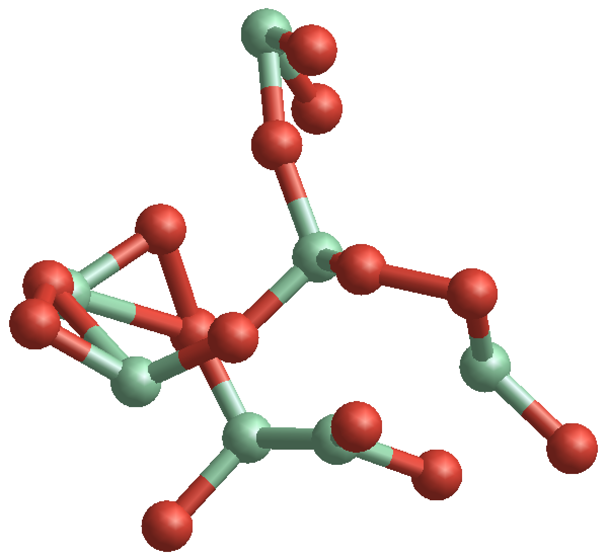
(a)

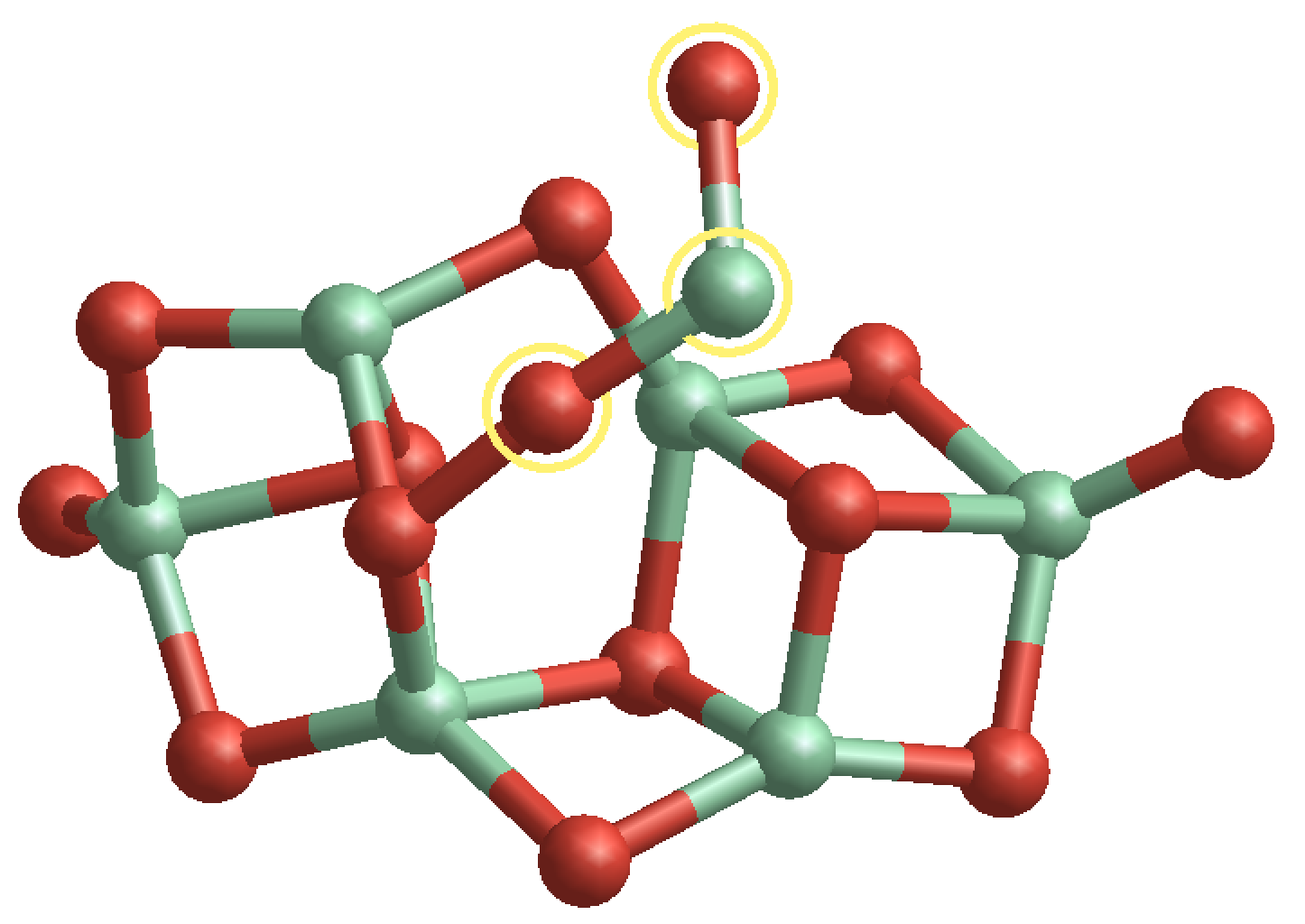
(b)

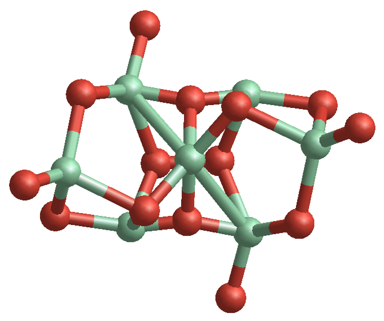
(c)

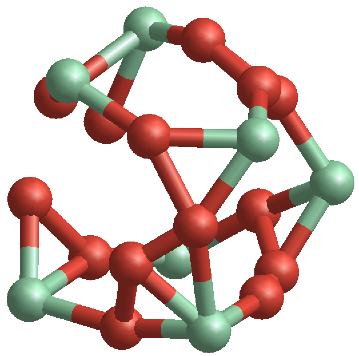
(d)

Figure 2: Examples for initial, unoptimized cluster geometries of size $N=7$, generated (a) randomly, (b) from known cluster with additional monomer (marked with yellow circles), (c) from a mirrored cluster of size $N=3$ with an additional monomer in the center, and (d) from $N=7$ monomers evenly distributed on a sphere.

2.2 Density functional theory

To accurately describe a cluster, a large number of interactions, including quantum-mechanical ones, need to be taken into account. We employ density functional theory (DFT) (see Appendix A.1) as a method to solve the Schrödinger equation approximately and determine zero-point energies, vibrational frequencies and rotational constants of our clusters. Density functional theory is parameterised through the choice of a functional and a basis-set, which has a large impact on the resulting quantities. It is therefore essential to select an appropriate functional and basis-set for our purpose.

2.3 Finding the ideal Functional and basis set

For the calculations at the Density Functional level of theory (DFT), the Gaussian16 (Frisch et al., 2013) program is used. It is desirable to use a model parameterisation that agrees with measured data. In order to determine the DFT parameterisation, in the form of a combination of functional and basis set, that most closely resembles measured data, the results are compared to experimentally derived data for the zero-point energy (Malcolm W. Chase, 1998), vibrational frequencies (Malcolm W. Chase, 1998) and rotational frequencies (Brünken et al., 2008) for the TiO₂ monomer molecule.

Approach for TiO₂:

The tested functionals include 2 GGA DFT functionals, 12 hybrid functionals with included Hartree-Fock exchange and 3 Complete Basis Set (CBS) methods listed in Table 1. The functionals were selected to cover a broad range of theoretical approaches as well as with regards to their availability within Gaussian16. Although there are no interactions within our clusters that stem from non-bonded interactions, we find that empirical damping coefficients as described by Grimme et al. (2011) improve the overall accuracy of our calibration. The EmpiricalDispersion=GD3BJ keyword is therefore used if available. We note that the use of an empirical dispersion does not originate from a physical or chemical consideration. Employing a similar approach in the selection of basis sets, a total of 129 candidate combinations of functionals and basis sets is produced (Table 1). For each of the combinations Gaussian16 is used to perform an optimisation of the TiO₂ monomer as well as a zero-point energy calculation for the Titanium and Oxygen atoms respectively. The resulting energies for the individual functionals and basis sets are compared with the experimental data found in the JANAF-NIST tables. All 129 functional/basis set combinations are evaluated according to their binding energy for the TiO₂ molecule calculated at a temperature of $T=0$K. The binding energy of the monomer (TiO₂) is calculated according to

$$E_{\rm bind}(\mathrm{TiO_{2}})=E_{\rm ZP}(\mathrm{TiO_{2}})-E_{\rm ZP}(\mathrm{Ti})-2\,E_{\rm ZP}(\mathrm{O})$$ (1)

and can now be compared to experimental values (Table 2, 4th column). $E_{\rm ZP}$ denotes the zero-point energy, i.e. the energy of the system at rest in its ground electronic state.
Further values that are known from experiments are the vibrational frequencies $\nu_{1}$, $\nu_{2}$, and $\nu_{3}$ (Malcolm W. Chase, 1998) and the rotational constants $A_{\rm rot}$, $B_{\rm rot}$, and $C_{\rm rot}$ (Brünken et al., 2008) of the TiO₂ monomer. These quantities are also a result of the DFT calculations and the derived thermochemical properties depend on them (Eq. 24). They are therefore used to further constrain which of the candidate combination of functional and basis set is best suited for modeling TiO₂ clusters. For both, the vibrational frequencies and the rotational constants, the quality of an individual candidate combination is assessed through a deviation parameter. Since the smallest deviation of the DFT results from the experimental data is desired, these deviation parameters are computed by taking the root sum squared of all relative deviations of the DFT results from the experimental data for the vibrational frequencies and the rotational constants, respectively (Table 2, 5th and 6th column). For the vibrational frequencies this parameter (Vibrational frequency deviation, VFD) is therefore calculated through:

$$\mathrm{VFD}=\sqrt{\sum_{i=1,..,3}\left(\frac{\nu_{i,DFT}-\nu_{i,Exp}}{\nu_{i,Exp}}\right)^{2}}$$ (2)

and equivalently for the rotational constants (Rotational constant deviation, RCD):

$$\mathrm{RCD}=\sqrt{\sum_{i=A,B,C}\left(\frac{i_{rot,DFT}-i_{rot,Exp}}{i_{rot,Exp}}\right)^{2}}$$ (3)

Using the Gaussian16 outputs for the zero-point energy of atomic oxygen, $E_{\rm ZP}(\rm O)$ [$\mathrm{kJ/mol}$], atomic titanium, $E_{\rm ZP}(\rm Ti)$ [$\mathrm{kJ/mol}$], and the titanium dioxide monomer, $E_{\rm ZP}(\rm TiO_{2})$ [$\mathrm{kJ/mol}$], the binding energy of the monomer is calculated and compared to the literature value from the JANAF-NIST tables. Since the JANAF-NIST tables have an accuracy for the binding energy of 4 $\mathrm{kJ/mol}$ (Malcolm W. Chase, 1998), the selection is narrowed down to all candidate combinations that fall within this uncertainty. This decreases the number of candidate combinations of functionals and basis sets from 192 to 16 (Table 2). Lastly, the runtime for each monomer calculation on a single node (32 cores) is determined, as computational speed and efficiency is desirable.

The thermochemical quantity of interest is the Gibbs free energy of formation $\Delta_{f}G^{\circ}(N)$, which is needed to compute nucleation rates (See Eq. 9 & 17). The molecular system properties that go into computing the Gibbs free energy are the zero-point energy, the vibrational frequencies, the rotational constants and spin multiplicities (Appendix C). The latter do not impact our results as we assume closed shell singlet clusters throughout our calculations.

The candidate combination of functional and basis set that has the smallest deviations from the experimentally known values for the zero-point energy, vibrational levels and rotational constants is considered optimal. The B3LYP functional in combination with the cc-pVTZ basis set and empirical GD3BJ dispersion (Grimme et al., 2011) has the lowest deviation from the experimental values for the zero-point energy and the vibrational frequencies, and the second lowest value for the rotational constant deviation. Therefore, B3LYP/cc-pVTZ represents the most suitable choice for the calibration of approaches with a lower level of complexity (Sect. 2.4.1) as well the final optimisation of our candidate clusters (Sect. 2.5). Additionally, it is desirable to reduce computational cost. In order to achieve that, the fastest configuration that falls within the 4 $\mathrm{kJ/mol}$ threshold, the B3LYP functional in combination with the def2svp basis set, is chosen to pre-optimise candidate geometries. This allows the final optimisation with the cc-pVTZ basis set to be completed in fewer steps, leading to overall lower computational cost. The CCSD(T) method is known as the gold-standard in computational quantum chemistry and has been the method of choice in quantum chemistry (Čížek, 1969; Purvis & Bartlett, 1998; Ramabhadran & Raghavachari, 2013; Nagy & Kállay, 2019). However, these calculations require large amounts computational resources and are prohibitive for larger molecular systems such as nano-sized clusters. Therefore, we performed CCSD(T)/6-311+G(2d,2p) single point calculations for the GM candidates with the smallest cluster sizes of $N$=1-4, and compare the 0K binding energies with our results from hybrid DFT (B3LYP/cc-pVTZ with empirical dispersion). The first thing to note is that CCSD(T) calculation results deviate from experimental results for the binding energy of the monomer by $\approx 90\frac{\mathrm{kJ}}{\mathrm{mol}}$, which is not adequate for our calibration purposes. When comparing the binding energy ratios to the monomer, $E_{bind,N}/E_{bind,1}$, the values for our DFT calculations do not differ by more than $2\%$ from the CCSD(T) values. We therefore conclude that calibration of our method with the experimentally determined properties of the monomer is sufficient. (Appendix B)

Table 1: All Gaussian16 functionals (methods) and basis sets considered when searching for the closest representation of the JANAF-NIST experimental values.

GGA Functionals
B97D3	[Grimme et al. (2011)]
TPSSTPS	[Tao et al. (2003)]
Hybrid Functionals
B3LYP	[Becke (1993b)]
B2PLYPD3	[Goerigk & Grimme (2011)]
BMK	[Boese & Martin (2004)]
PBE1PBE	[Adamo & Barone (1999)]
LC-wPBE	[Vydrov & Scuseria (2006)]
CAM-B3LYP	[Yanai et al. (2004)]
APFD	[Austin et al. (2012)]
M11	[Peverati & Truhlar (2011)]
MN12SX	[Peverati & Truhlar (2012)]
HSEH1PBE	[Heyd et al. (2003)]
X3LYP	[Xu & Goddard (2004)]
M06	[Zhao & Truhlar (2008)]
CBS extrapolations
CBS-4M	[Montgomery et al. (2000)]
CBS-QB3	[Montgomery et al. (2000)]
ROCBS-QB3	[Wood et al. (2006)]
basis sets
def2svp	[Weigend (2006)]
Def2TZVP	[Weigend (2006)]
def2svpp	[Weigend (2006)]
Def2TZVPP	[Weigend (2006)]
cc-pVDZ	[Wilson et al. (1996)]
cc-pVTZ	[Wilson et al. (1996)]
AUG-cc-pVDZ	[Wilson et al. (1996)]
AUG-cc-pVTZ	[Wilson et al. (1996)]
6-311+G*	[Curtiss et al. (1995)]

Table 2: Candidate combinations for functional and basis set with a zero-point binding energy deviation $\lvert E_{bind,JANAF}-E_{bind,DFT}\rvert<4\mathrm{kJ/mol}$, sorted by vibrational constant deviation.

Rank	Functional	basis set	Deviation from Janaf-Nist [kJ/mol]	Vibrational frequency deviation (VFD)	Rotational constant deviation (RCD)	Core computational time [s]
1	B3LYP	cc-pVTZ	0.22	0.096	0.029	1251.6
2	B3LYP	AUG-cc-pVDZ	1.12	0.1	0.025	1229.6
3	B3LYP	Def2TZVPP	3.11	0.101	0.03	978.8
4	X3LYP	cc-pVDZ	0.47	0.12	0.042	1683.9
5	APFD	cc-pVTZ	3.18	0.136	0.05	1842.8
6	APFD	AUG-cc-pVDZ	2.79	0.138	0.047	1462.7
7	M06	Def2TZVP	2.75	0.141	0.045	748.2
8	PBE1PBE	cc-pVDZ	2.99	0.156	0.063	1097.7
9	M11	6-311+G*	1.59	0.157	0.087	837
10	M11	AUG-cc-pVTZ	2.14	0.159	0.079	6287.7
11	M11	cc-pVTZ	2.4	0.16	0.084	3416.2
12	M11	AUG-cc-pVDZ	3.88	0.163	0.086	2879.9
13	M11	Def2TZVP	1.64	0.171	0.088	841.9
14	B3LYP	def2svp	1.04	0.19	0.06	440.1
15	LC-wPBE	Def2TZVP	2.81	0.194	0.086	765.3
16	APFD	def2svp	3.36	0.228	0.079	440.2

2.4 Calibration of force fields and DFTB

2.4.1 Calculation of known small clusters and isomers

After the selection of the ideal combination of functional and basis set, judged by its ability to closely match the experimentally derived properties of TiO₂, it is used to calculate the binding energies and geometries of the global minimum structures of the clusters of $N=2\,\ldots\,6$. The initial geometries for these calculations are sourced from Berardo et al. (2014) and Lamiel-Garcia et al. (2017). Additionally, the binding energy and geometry for several energetically less favorable isomers for each size is calculated (Table 3). This is done so that the accurate depiction of the energetic ordering of isomers of the same size by force field and DFTB+ models can be ensured.

Table 3: Number of isomers for each cluster size optimised at the DFT level, used to calibrate force field and DFTB models.

Cluster size $N$	Number of isomers
2	3
3	9
4	17
5	14
6	14

2.4.2 Force fields

In order to save computational time, it is beneficial to be as efficient as possible in the optimisation process towards local and global potential minima for candidate isomers. For example, a titanium-dioxide cluster of size N=12 ($(\mathrm{TiO}_{2})_{12}$) has 36 atoms and thereby 3x36 = 108 degrees of freedom. The number of possible geometries is simply too large to be modeled at a feasible computational cost for a large number of clusters. Therefore a modelling approach is employed, that describes the interactions between individual atoms through an interatomic Buckingham pair potential including the Coulomb potential. (Appendix A.2) There are several parameterisations for Ti–O systems provided in previous studies, e.g. Matsui & Akaogi (1991) or Lamiel-Garcia et al. (2017). However, we find that neither of them are well suited for our purposes as they do not accurately depict the B3LYP/cc-pVTZ energetic ordering within isomers of the same size $N$. To find a force field prescription that reflects the experimental data available for TiO₂ to the extent possible, a search is conducted for a set of Buckingham parameters that reproduce the binding energies and average bond distance of the smallest clusters calculated at the start of Sect. 2.4.1.

Approach to (TiO₂)_N:

The program used to calculate the energy as well as the bond distance is the General Utility Lattice Program GULP (Gale & Rohl, 2003). The optimise keyword is used in a constant pressure environment (conp) to optimise the DFT optimised clusters and determine their binding energies for each combination of parameters. The parameters that need to be determined in Eq. 18 are the charges of Ti and O, and the Buckingham pair parameters $A$, $B$, and $C$ for each of the relevant interactions, Ti-Ti, O-O, and Ti-O. Since overall charge neutrality needs to be conserved, the charge of Ti is directly coupled to the charge of O by a factor of -2, i.e. there are two negatively charged Oxygen anions for every positively charged Titanium cation. For the TiO₂ molecule the authors find low formal charges. Mulliken charge analysis of the smallest cluster sizes (N=1-4) reveal average Ti charges of less than +1e. The parameterisation therefore has 10 free parameters, three from each of the interactions, i.e. Ti-Ti, O-O, and Ti-O, plus the charge. To find the ideal parameter set all interaction parameters as well as the charge are varied freely and the scipy.optimise differential evolution algorithm (Storn & Price, 1997) is used to find the set of parameters that deviates the least from our calculated binding energies and average bond distances, as well as reproduces the energetic ordering of isomers of the same size. (Appendix D.1) With this physically consistent set of parameters the potential energy of any Ti-O system, i.e. any TiO₂ cluster geometry, can now be accurately predicted, requiring little computational power. This approach of searching for candidate structures with the application of a Buckingham pair potential has been used before, e.g. in Gobrecht et al. (2018) for aluminium oxide, in Cuko et al. (2017) for hydroxylated silica clusters and for titanium dioxide in Lamiel-Garcia et al. (2017).

The seed structures are optimised using our re-parametrised force field as the first step in our hierarchical approach. To even further increase the structural complexity of our searches, a basin-hopping algorithm as described by Wales & Doye (1997) is employed. It is used in its implementation in the ase Python package (Hjorth Larsen et al., 2017) to optimise the geometries of all the seed structures. The potential energy calculation at each step of the optimisation is done through GULP with our parameterisation of the force field. After the force field optimisation the candidate geometries are analysed further in Sect. 2.4.3.

2.4.3 Density Functional based Tight Binding (DFTB)

From the geometry optimisation with the force field approach (Sect. 2.4.2) 2000 candidate geometries at local potential minima for each small cluster size, $N=3-7$, and 10000 candidate geometries for each large cluster size, $N=8-15$, are obtained. However, the Buckingham-Coulomb pair potential does not describe the interaction between electrons and their related orbitals. More precisely, only interactions between Ti cations, O anions, and themselves are taken into account. The interaction of (binding) electrons and the electron correlation is neglected. Still, it serves the purpose of optimising the candidate geometries on a approximate and simplified PES. The potential energies of the (TiO₂)_$N$ cluster candidates are not accurate, because, among other reasons, the force field approach considers single point charges instead of a charge distribution of each ion in the cluster. It is therefore a reasonable assumption that the binding energies of these clusters and their energetic ordering can be improved by an intermediate optimisation step with a more accurate description accounting for electronic orbitals. This is done to get a more accurate energetic ordering of the candidate clusters, so the best set of candidate clusters is chosen to be optimised with computationally expensive all-electron DFT calculations (see Section 2.5). For this intermediate step density functional based tight binding (DFTB, Appendix A.3) is chosen. The choice is made because in both complexity and computational cost, DFTB models fall in between the descriptions offered by force fields and all-electron DFT models (Hourahine et al., 2020). The parameterisation of the exchange-correlation functional is not included within the DFTB model and is done through choosing an appropriate set of Slater-Koster files. These files relate to integrals and contain sets of functions that describe the exchange-correlations part of interactions between two atomic species (i.e. chemical elements). The database at www.dftb.org hosts three different sets that describe the interaction of titanium and oxygen: matsci (Luschtinetz et al., 2009), a general purpose material science set, trans3d (Zheng et al., 2007), a set describing transition metal elements in biological systems, and tiorg (Dolgonos et al., 2010), a set for describing Ti bulk, TiO₂ bulk, TiO₂ surfaces, and TiO₂ with organic molecules. In order to find an exchange-correlation parameterisation that best describes small TiO₂ clusters, our test clusters calculated in Sect. 2.4.1 are used to test all three sets of Slater-Koster files.

Approach to (TiO₂)_N:

The DFTB calculations are done using the DFTB+ program (Hourahine et al., 2020). For the calibration of the DFTB method the energies calculated for geometries in Sect. 2.4.1 are used. For clusters of $N=3\,\ldots\,6$, equivalent to our approach in calibrating our force fields, DFTB+ is used to calculate the total energy for all the isomers with each of the three different sets of Slater-Koster files. Afterwards it is tested which of these reproduces the energetic ordering of the isomers found with all-electron DFT calculations. If two of the Slater-Koster files perform identically in this regard, the one is chosen that better approximates the absolute values of the binding energies. The matsci (Luschtinetz et al., 2009) set of Slater-Koster files is found to perform the best for the purpose of this paper. (Appendix D.2) Subsequently this set of Slater-Koster files is used to describe the exchange correlation in the further evaluation and optimisation of the seed structures from Sect. 2.4.2. To enable direct comparison to the results of DFTB+ optimised isomers, the potential energy for each of the candidate geometries is obtained by performing a single-point energy calculation with DFTB+. Next, an identical calculation for atomic Ti and atomic O is performed, in order to obtain their respective potential energies. The binding energy of a (TiO₂)_$N$ cluster can then be calculated by substracting the individual contributions, analogous to Eq.1:

$$\mathrm{E_{Bind}((TiO_{2})}_{N})=\mathrm{E_{Pot}((TiO_{2})}_{N})-N\cdot\mathrm{E_{Pot}(Ti)}-2\cdot N\cdot\mathrm{E_{Pot}(O)}$$ (4)

This calculation is performed for each of the candidate geometries obtained from Sect. 2.4.2. Each of the candidate geometries is then optimised using the ConjugateGradient method, making use of its implementation within DFTB+, and are again ordered according to their binding energies calculated with Eq. 4. Since the randomisation of seed structures is not ideal, there will be duplicates among the optimised geometries. In order to filter them out any two candidates with a binding energy difference of $\Delta\mathrm{E_{Bind}}\leq 0.01\mathrm{eV}$ are analysed with regards to their similarity. For that the mean of all inter-atomic distances within the cluster is calculated, giving a size parameter $R$. If the average inter-atomic distance of the two clusters is closer than $\Delta R\leq 0.01$Å, the two clusters are found to be duplicates and one of them is removed from the process. After removing the duplicate candidate geometries, the lowest energy clusters for each size and used in our final step, optimisation with all-electron DFT in Sect. 2.5.

2.5 Global minima search with DFT

The energetically most favourable isomers found with DFTB (see Sect. 2.4.3) are further optimised using Gaussian16. In order to reduce total computational time, a first optimisation is performed with the B3LYP/def2svp functional/basis set combination with empirical dispersion as described by Grimme et al. (2011). After this step, the final optimisation is done with the B3LYP/cc-pVTZ functional/basis set combination, also with empirical dispersion (Sec. 2.3). For all these isomers, a frequency analysis is carried out using the same functional/basis set, in order to make sure that the isomer is a true minimum and to exclude transition states. In addition, we calculate the final energies as well as rotational constants needed to determine the thermochemical properties we are interested in. The thermochemical properties entropy $S^{\circ}(N)$ $\left(\frac{\mathrm{J}}{\mathrm{mol}\cdot\mathrm{K}}\right)$, change of enthalpy ddH $\left(\frac{\mathrm{kJ}}{\mathrm{mol}}\right)$ and Gibbs free energy of formation $\Delta_{f}G^{\circ}(N)$ $\left(\frac{\rm kJ}{\rm mol}\right)$ are calculated from the output of the DFT optimisations using the RRHO approximation as implemented within the thermo.pl (Irikura, 2002) code.

3 Results

3.1 Force field optimised clusters

The new parameterisation (Table 9) for the Buckingham-Coulomb force field is used to optimise the geometric seed structures (Sect. 2.1). The algorithm used for this search is a basin hopping algorithm described by Wales & Doye (1997). The energy evaluation within this algorithm is done using GULP with the new set of parameters. At each step of the algorithm a local energy minimisation using the FIRE algorithm (Bitzek et al., 2006) is performed. This algorithm is designed specifically for optimisation of atomistic systems towards their closest local minimum. A numerical ’temperature’ of $T=100$ within the basin-hopping algorithm is chosen to allow for the exploration of nearby local minima in order to find the deepest potential well in the vicinity. This temperature is not a physical temperature, but influences the rejection criterium within the algorithm. All seed structures created in Section 2.1 for each cluster size $N$ = 3,…,15 are optimised with this algorithm.

3.2 DFTB energy calculations and optimisation

A zero-point energy calculation is performed for all cluster geometries calculated in Sect. 3.1 and their binding energies are calculated according to Eq. 4 (Fig. 3). Then each of these cluster geometries is optimised, minimising their potential energy, with the DFTB description of interactions. A ConjugateGradient optimisation algorithm (Hestenes & Stiefel, 1952) is used and the binding energies of the optimised clusters are calculated again (Fig. 4). A comparison of Figures 3 and 4 demonstrates the approximative character of the force field approach, as a seemingly broad variety of local minima for small clusters disappears with the introduction of higher complexity in the form of DFTB. The energy levels become discrete, many different cluster geometries from the force field approach produce the same geometry after further optimisation. To find potentially new global minimum (GM) structures, all known literature GM clusters are optimised and their binding energies calculated with the DFTB approach for comparison. For each size, any unique cluster that has a higher binding energy than the known literature GM is categorised as a candidate for a new GM. Additionally, the 10 isomers with binding energies closest to that of the literature GM are considered. These isomers (Table 4) are passed on to be optimised with all-electron DFT calculations.

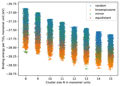
Figure 3: Binding energy per TiO₂ monomer unit for small ($N=3-7$, left) and large ($N=8-15$, right) clusters for the 90% of the most favourable clusters after optimisation with the force field approach. Individual clusters are color coded by method of creation of the candidate cluster (Sec. 2.1). A random spread along the x-axis has been added to enable comparison between clusters at similar energies.

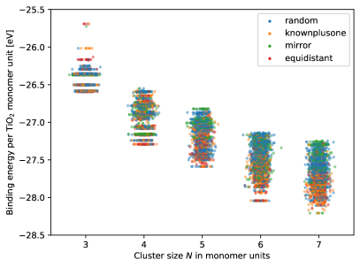
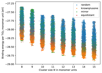
Figure 4: Binding energy per TiO₂ monomer unit for small ($N=3-7$, left) and large ($N=8-15$, right) clusters for the best 90% of clusters after optimisation with the DFTB approach. Individual clusters are color coded by method of creation of the candidate cluster (Sec. 2.1). A random spread along the x-axis has been added to enable comparison between clusters at similar energies.

Table 4: Number of GM candidates, i.e. cluster candidates with a higher binding energy than the literature GM after DFTB optimisation, and number of isomers calculated with all-electron DFT calculations for each size.

Size	GM candidates	Isomers
3	3	10
4	2	10
5	1	10
6	0	10
7	4	10
8	1	10
9	3	10
10	3	10
11	6	10
12	2	10
13	2	10
14	0	10
15	0	10

3.3 Comparison of candidate creation approaches

In this section, the performance of the different methods for creation of candidate geometries (see Sec. 2.1) is discussed. Additionally the necessity for cluster geometries from literature is assessed, to establish if the method is capable of operating without prior knowledge of particularly favourable cluster geometries. The parameter space that needs to be covered to find all possible geometric configurations increases dramatically with cluster size N. One metric to look at is the number of duplicate isomers. Table 5 lists the number of created candidates and resulting unique clusters for all cluster sizes $N$ considered. For the small clusters many duplicates are found, as the parameter space is small and many created geometries share a nearby potential minimum. As the size of the clusters grows, the number of identical geometries falls, creating more unique clusters per candidate. A plateau of unique clusters is reached from size 12, from where about 68% of the created clusters are unique. As larger clusters have a larger parameter space for possible geometric configurations, the trend of an increasing number of unique clusters is expected to continue. The resulting plateau therefore signals a limit of the current methods to fully explore the parameter space of clusters larger than $N=12$.

Table 5: Number of created candidate geometries, unique cluster geometries after DFTB optimisation and percentage of unique clusters per created candidate for all sizes $N$

Size	Candidates	Unique clusters	Unique clusters
			per candidate [%]
3	2000	150	7.5
4	2000	264	13.2
5	2000	606	30.3
6	2000	991	49.6
7	2000	1054	52.7
8	10000	5204	52.0
9	10000	5540	55.4
10	10000	6159	61.6
11	10000	6178	61.8
12	10000	6785	67.9
13	10000	6718	67.2
14	10000	6784	67.8
15	10000	6793	67.9

Two out of the four approaches used in this work rely on known cluster geometries that are reported in the literature, in order to produce cluster candidates (Known+1 and Mirror, methods 2 and 3 in Sec. 2.1, referred to as dependent methods), while the other two (Random and Equidistant, methods 1 and 4 in Sec. 2.1, referred to as independent methods) need only information about the monomer. Figure 5 and Table 6 show the 50 best, i.e. highest binding energy, candidates and their creation methods. For small clusters $N=3-6$ the independent methods produce the majority of the 50 clusters with the highest binding energy. These independent methods also find the GM candidates reported in the literature for $N=3-6$, which are needed for calibration. For larger clusters the dependent methods perform better. The random generation method only produces a single of the 50 energetically most favorable clusters for $N$ $>$ 10. This is because the PES is very large and complex at these sizes and can not be sufficiently explored by a random walk. Therefore, the methods that contain prior information about stable configurations, such as the dependent methods show an enhanced performance. The equidistant method is similar, as it also does not rely on previously reported favourable isomers. That is why for $N$ $>$ 10 the dependent methods make up far more of the energetically most favourable clusters. More elaborate methods to create first-guess cluster geometries are available through, for example, Gaussian process regression (e.g., Meyer & Hauser (2020)). For the present work, the choice was made to apply simple but fast methods and comparisons to more complex approaches are desirable in future works.

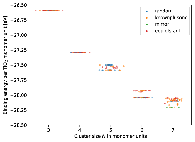
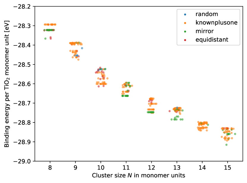
Figure 5: Binding energy per monomer unit for small ($N=3-7$, top) and large ($N=8-15$, bottom) clusters for the best 50 clusters after optimisation with the DFTB approach. Individual clusters are color coded by method of creation of the candidate cluster (Sec. 2.1). A random spread along the x-axis has been added to enable comparison between clusters at similar energies.

Table 6: The 50 lowest energy clusters after DFTB optimisation for which the un-optimised geometry guess were created by four different procedures (random, mirror, known+1, equidistant).

Size	Random	Mirror	Known+1	Equidistant
3	11	0	14	25
4	10	0	6	34
5	19	0	17	14
6	13	3	18	16
7	6	5	28	11
8	0	22	15	13
9	4	2	41	3
10	5	2	30	13
11	0	25	23	2
12	0	14	30	6
13	1	16	28	5
14	0	2	48	0
15	0	12	36	2

3.4 All-electron DFT calculations

All candidate geometries from Table 4, as well as all literature GM geometries from Berardo et al. (2014) and Lamiel-Garcia et al. (2017) are pre-optimised using Gaussian16 with the B3LYP functional, def2svp basis set and empirical dispersion. Afterwards they are optimised and a frequency analysis is performed with the best performing combination found in Sec. 2.3, B3LYP/cc-pVTZ with empirical dispersion. For all isomers, the binding energies are calculated according to Eq. 4 and their respective geometries can be found in electronic form at the CDS via anonymous ftp to or via . For cluster sizes $N=3-10$, the GM candidates predicted in the literature were found among the candidate geometries after DFTB optimisation. For cluster size $N=11$ the predicted GM was found among the candidate geometries after DFT optimisation. For cluster sizes $N=$ 12,14 and 15, the predicted GM were not found among the candidate geometries and no more favourable isomer, i.e. with an even lower potential energy, was found either. This is most likely due to the fact that the seed-creation approaches employed here are not well suited to cover the large parameter space for these large clusters within 10000 candidates, as was mentioned in Sec. 3.3. For $N=13$, we present a new global minimum candidate structure (Fig. 6), which was created through the mirror creation process (Method 3 in Section 2.1). Its potential energy is $0.5\frac{\mathrm{kJ}}{\mathrm{mol}}$ per monomer unit lower than the previous lowest-lying isomer reported by Lamiel-Garcia et al. (2017). This difference is lower than the typically assumed accuracy for DFT calculations of $4\frac{\mathrm{kJ}}{\mathrm{mol}}$ per monomer unit. This supports the need to study energetically similar isomers for each cluster size, as either could play a role in the nucleation process.

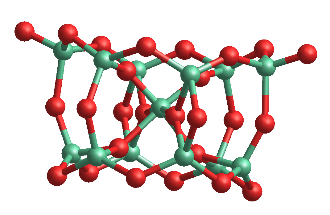
Figure 6: New global minimum structure for (TiO₂)₁₃, binding energy: E${}_{binding}=-1782.96\frac{\mathrm{kJ}}{\mathrm{mol}}$ per monomer unit.

In thermochemical processes such as nucleation, the most relevant isomer for each cluster size is assumed to be the energetically most favourable one. Any less favourable, meta-stable isomer that forms relaxes into that global minimum, given sufficient time for the relaxation. To compare the thermochemical properties, the thermo.pl program is used to calculate the entropy S [J mol^-1 K^-1], change of enthalpy $d\Delta H$ [kJ mol^-1] and Gibbs free energy of formation $\Delta_{f}G^{\circ}$ [kJ mol^-1] for three different sets of clusters:

1. The GM for each size, including cluster geometries reported in the literature, calculated with B3LYP/def2svp and empirical dispersion

2. The GM for each size, including cluster geometries reported in the literature calculated with B3LYP/cc-pVTZ and empirical dispersion

3. The GM for each size, only including cluster geometries that have been found in this work, calculated with B3LYP/cc-pVTZ and empirical dispersion

This is done in order to compare the impact of the choice of functional/basis set on the zero-point energies and the thermochemical properties to the impact of the completeness of the GM search for the cluster geometries. The complete thermochemical tables for set 2 are only available in electronic form at the CDS via anonymous ftp to or via .

4 Astrophysically relevant (TiO₂)_N properties

In previous sections, we have derived the fundamental quantities including the zero-point energy of TiO₂ clusters. The thermochemical properties of interest for astrophysical studies are:

1. S(T), Entropy [J mol^-1 K^-1]

2. d$\Delta H$(T), change in enthalpy [kJ mol^-1]

3. $\Delta_{f}G^{\circ}$(T), Gibbs free energy of formation [kJ mol^-1].

The following sections will present TiO₂ in the context of the gas phase, and TiO₂ clusters as a promising precursor of TiO2 dust formation, and the derivation of their thermochemical properties, especially the size- and temperature-dependent Gibbs free energy of formation $\Delta_{f}G^{\circ}(N,T)$, that are relevant for cloud formation modelling in exoplanets and brown dwarfs as well as for dust formation modelling in AGB stars and supernova ejecta.

4.1 Thermodynamical relevance of TiO₂ in hot Jupiters

In order to assess the relevance of TiO₂ for cloud formation in the atmospheres of hot Jupiters or for dust formation in an AGB envelope, it is necessary to know the thermodynamic quantity ranges in which TiO₂ is the most abundant Titanium-bearing molecule. For this we apply the gas-phase equilibrium chemistry code GGChem from Woitke et al. (2018). TiO₂ is the most abundant Titanium-bearing molecule at a pressure of $10^{-3}$ bar in the low-temperature regime i.e. for T$<1$200 K (Figure 7). Less complex Ti-bearing species dominate the chemical Ti- content with increasing temperatures until Ti⁺ is the dominating Ti species at $T>3500$K. Figure 8 presents the GGChem model as a 2D ($p_{\rm gas}$, $T_{\rm gas}$) plane with a 1D atmospheric $p_{\rm gas}$, $T_{\rm gas}$ profile of a hot Jupiter superimposed. The profile corresponds to a model of a hot Jupiter with $T_{\rm eff}=1600$K and $\log(g)$ = 3, orbiting a G star with $T_{*}=5650$K (Baeyens et al., 2021) which was extrapolated to pressures of $10^{-14}$ bar. The model is plotted at four different locations on the planet: the substellar and anti-stellar point, and the morning and evening terminator for this hot Jupiter.

Only at the substellar point for the model atmosphere ($T_{\rm eff}=1600K$) TiO₂ is not the most abundant Ti-bearing species at any pressure-level, except at a thin layer of the atmosphere at $10^{-2}$ bar. For the anti-stellar point and morning terminator, TiO₂ is the dominant Ti-bearing molecule in the upper atmosphere. Only in the lower atmosphere at around $10^{-1}$ bar, other molecules such as TiO and later atomic Ti become dominant. For the evening terminator, TiO₂ becomes less abundant than TiO at a pressure level of $\sim 10^{-2}$ bar. Moreover, we note that the (TiO₂)_N cluster ionization energies of 9.3-10.5 eV are too high to affect related abundances and the TiO_N nucleation in exoplanet atmospheres(Gobrecht et al., 2021b). This strengthens the argument that TiO₂ is the most relevant Ti-bearing molecule in the upper atmosphere, which is were cloud formation is expected to take place.

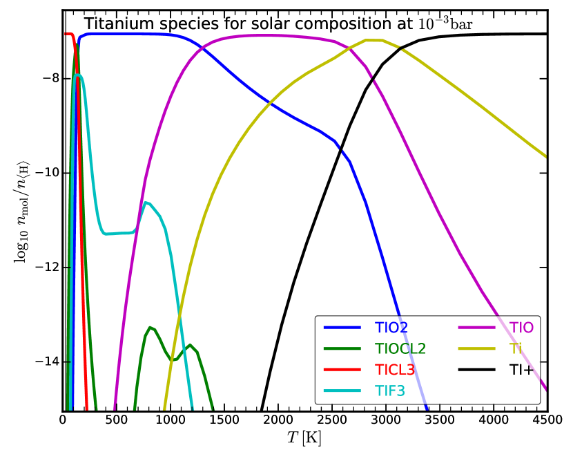
Figure 7: Concentrations of Titanium containing molecules in gas-phase chemical equilibrium at 10^-3 bar. Solar element abundance are assumed. TiO₂ is the most abundant Ti-binding species up to 1200K and the second most abundant species up to 1800K.

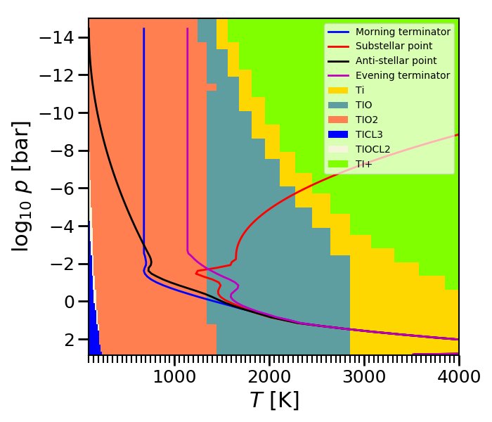
Figure 8: Most abundant gas phase molecules containing Titanium from a gas of solar composition using equilibrium chemistry. Pressure temperature profiles for a hot Jupiter atmospheres with $T_{\rm eff}=1600$K included, probing the atmosphere at four distinct locations.

4.2 Surface tension of TiO₂

In classical and modified classical nucleation theory, the impact of the Gibbs free energy of formation $\Delta_{f}G^{\circ}$ on the nucleation process is modeled through the surface tension $\sigma_{\infty}$ of the bulk solid (Gail & Sedlmayr, 2013). The fact, that the surface tension is different for small a finite size leading to significantly different geometries and properties than the bulk, is neglected. It is however possible to find a surface tension that is valid for small clusters if individual cluster data are available. Here the approach by Jeong et al. (2000) as it was applied by Lee et al. (2015) is followed, in which the dependence of the Gibbs free energy of formation on the cluster size is linked to the surface tension $\sigma_{\infty}$ through:

with cluster size $N$, the Gibbs free energy of formation of a cluster of size N, $\Delta_{f}G^{\circ}(N)$, the Gibbs free energy of the monomer $\Delta_{f}G^{\circ}(1)$, the Gibbs free energy of the bulk phase $\Delta_{f}G^{\circ}_{1}(s)$, a fitting factor $N_{f}$ and

$$\theta_{\infty}=\frac{4\pi a_{0}^{2}\sigma_{\infty}}{k_{b}T}$$ (6)

Here $a_{0}$ is the theoretical monomer radius, which is derived from the bulk density of rutile and the molar mass through:

$$a_{0}=\left(\frac{3M_{TiO_{2}}}{4\pi\rho_{\rm Rutile}}\right)^{1/3}\simeq 1.956\times 10^{-10}m$$ (7)

The fitting factor $N_{f}$ is set to $N_{f}=0$, analogous to Lee et al. (2015). The Gibbs free energies for the monomer and for the bulk are known from experiment (Malcolm W. Chase, 1998), as are the values necessary to derive $a_{0}$. The Gibbs free energy of formation of the clusters is calcluated from the thermochemical values derived from our all-electron DFT calculations and consistently compared to the thermochemical clusterdata from the study by Lee et al. (2015).

That leaves $\sigma_{\infty}$ as the only free parameter, which is fit using Eq. 5. The left-hand side of Figure 9 compares the data from both functional/basis set combinations used in this work to the results from Lee et al. (2015). It becomes apparent that the choice of the functional and basis set influences the resulting thermochemical properties and therefore the surface tension given by the fit. In this work we get a different result for the surface tension than Lee et al. (2015) using their data. The result for the surface tension at $T=1000$K using all available GM data and the best performing functional/basis set combination is $\sigma_{\infty}=518\ \mathrm{erg\ cm^{-2}}$ (blue line in Fig. 9). In the right panel of Figure 9, the comparison is made between the fits for $\sigma_{\infty}$ using all available GM data (blue) and only the best candidates that were produced from candidates in this work (red). Both the data as well as the results for $\sigma_{\infty}$ vary only slightly, visible differences occurring for $N=14$ and $N=15$, where this work did not produce candidates that were identical or energetically close to the literature GM. The best fit value for $\sigma_{\infty}$ without using GM candidates found in the literature is $\sigma_{\infty}=525\ {\rm erg\ cm^{-2}}$, differing from the best fit value by only $7\ {\rm erg\ cm^{-2}}$. This indicates that the choice of functional and basis-set has a stronger impact on the resulting surface tension than finding the lowest-energy isomer for all sizes, given the extent of our searches.

Since potential minimum geometries that were missed all have lower enthalpies and therefore, presumably also lower Gibbs free energies, they can only lower the resulting surface tension. This approach therefore gives an upper limit for the surface tension $\sigma_{\infty}$.

The best fit value for the surface tension is found to be dependent on the temperature. Fig. 10 shows the best fit for a linear dependence of $\sigma_{\infty}$ on T for T = $500-2000$ K:

$$\sigma_{\infty}(T)=589.79-0.0708\cdot T$$ (8)

Studies have been conducted on the surface tension of bulk Rutile at room temperature (Kubo et al., 2007), finding a value of $\sigma_{\infty}(298.15\mathrm{K})=1001\ \mathrm{erg\ cm^{-2}}$ for the (011) lattice. The best fit for room temperature in this study gives a value of $\sigma_{\infty}(298.15\mathrm{K})=575.72\ \mathrm{erg\ cm^{-2}}$ for small (TiO₂)_N molecular clusters. The factor of almost two in surface tension for small clusters versus the bulk phase of TiO₂ makes it clear that the prior is recommended in all considerations regarding nucleation processes.

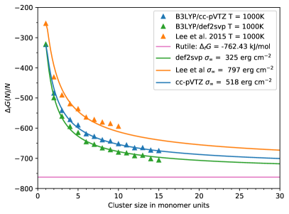
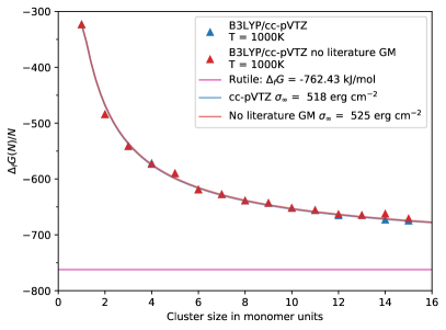
Figure 9: Gibbs free energy of formation per cluster size $N$ as a function of cluster size $N$ at a temperature of T = 1000K. For each approach a fit for $\sigma_{\infty}$ was calculated using eq. 5. Left: Comparison between resulting surface tensions for different sources of cluster data. The sources are Lee et al. (2015) for the orange line, DFT calculations with the fast basis set def2svp for the green line and DFT calculations with the accurate basis set cc-pVTZ for the blue line. Right: Comparison of the impact of isomer completeness on resulting surface tension. Both lines use thermochemical data derived from the accurate cc-pVTZ basis set DFT calculations. For the blue line the energetically most favoured isomer was chosen for all sizes, regardless of whether it was found by the approach in this paper or not. For the red line only outputs from this papers approach were used. As the resulting difference is small it becomes apparent that the choice of the basis set is more impactful than the completeness of the cluster geometries.

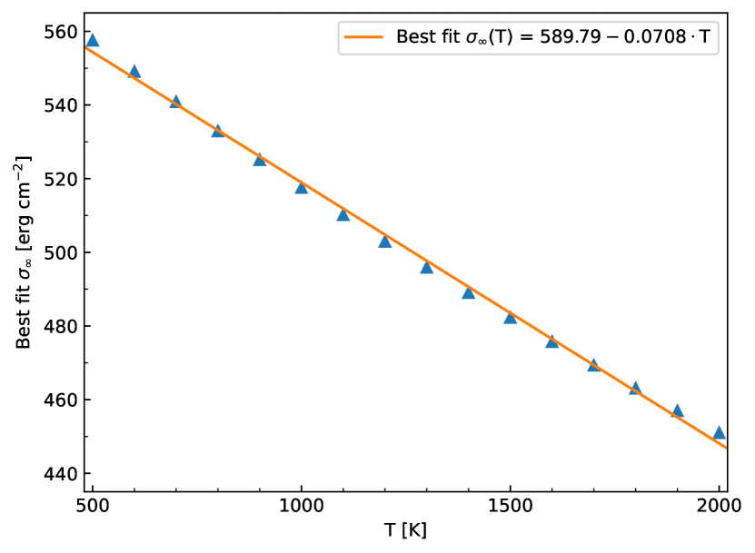
Figure 10: Dependence of the best fit for $\sigma_{\infty}$ on the temperature $T$. A linear regression has been applied.

4.3 Nucleation rates of TiO₂

To quantify the effect of the updated thermochemical cluster data on quantities relevant for cloud formation in exoplanet atmospheres, the nucleation rate for TiO₂ is calculated along the temperature pressure profile of the morning terminator of a hot Jupiter with an effective temperature of $T_{\mathrm{eff}}=1600$K and a surface gravity of $\log g=3$ (blue lines in Fig. 8). The gas phase composition is calculated with the equilibrium chemistry code GGChem.

4.3.1 Modified classical nucleation theory (MCNT)

In this work, the nucleation rates are computed analogously to Lee et al. (2015) for ease of comparison. The stationary, homogeneous, homomolecular nucleation rate in classical nucleation theory is calculated by:

$$\centering J^{c}_{*}=\frac{f^{\circ}(1)}{\tau_{gr}(r_{i},N_{*},T)}Z(N_{*})\exp\left((N_{*}-1)\ln S(T)-\frac{\Delta G(N_{*})}{RT}\right)\@add@centering$$ (9)

Here, $S(T)$ and $f^{\circ}(1)$ are the supersaturation ratio and monomer number density of TiO₂ respectively. $\tau_{gr}$ is the growth timescale, defined as:

$$\centering\tau_{gr}^{-1}=A(N)\alpha(N)v_{rel}n_{f}\@add@centering$$ (10)

with $A(N)=4\pi a_{0}^{2}N^{2/3}$ the effective cross-section of a spherical (TiO₂)_N cluster, $n_{f}$ the monomer number density ($n_{f}=f^{\circ}(1)$), the sticking factor $\alpha$, which is assumed to be $\alpha=1$, and the relative velocity $v_{rel}$, which is given for monomers with mass $m_{x}$ by the thermal velocity through:

$$\centering v_{rel}=\sqrt{\frac{kT}{2\pi m_{x}}}\@add@centering$$ (11)

Z(N) is the Zeldovich factor, which accounts for the contribution to nucleation from Brownian motion:

$$\centering Z(N_{*})=\sqrt{\frac{\theta_{\infty}}{9\pi(N_{*}{-1})^{4/3}}}\@add@centering$$ (12)

and in the final term, the Gibbs free energy $\Delta G(N)$ is approximated using modified classical nucleation theory, or MCNT, giving:

$$\centering\frac{\Delta G(N_{*})}{RT}=\theta_{\infty}(N_{*}-1)^{2/3}\@add@centering$$ (13)

with $\theta_{\infty}$ from Eq. 6. Equation 9 is evaluated at the critical cluster size $N_{*}$, which is given by:

$$\centering N_{*,\infty}=\left(\frac{\frac{2}{3}\theta_{\infty}}{\ln S(T)}\right)^{3}\ \ \ N_{*}=\frac{N_{*,\infty}}{8}+1\@add@centering$$ (14)

The critical cluster size is mainly influenced by the supersaturation of molecular TiO₂ at various temperature and pressure points. When TiO₂ is not supersaturated ($\ln S(T)<0$), N_∗ is negative (Eq 14), and consequently Eq. 13 has no real solution, leading to the absence of nucleation for the modified classical case at these temperature pressure points. Using Eq. 9, the classical nucleation rate was calculated for the given ($\rm p_{gas}$,$\rm T_{gas}$-profile using three different values for $\sigma_{\infty}$: The temperature dependent $\sigma_{\infty}$ from this work, the temperature dependent $\sigma_{\infty}$ from Lee et al. (2015) and a constant $\sigma_{\infty}=797$ erg cm^-2, derived from the re-fit to Lee’s cluster data in this work. Results can be found in Figure 11.

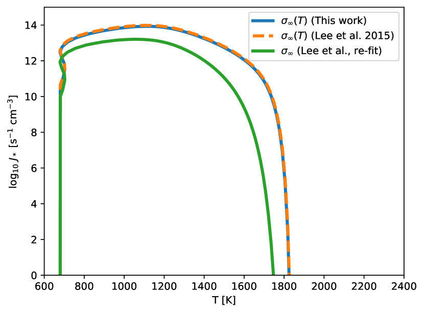
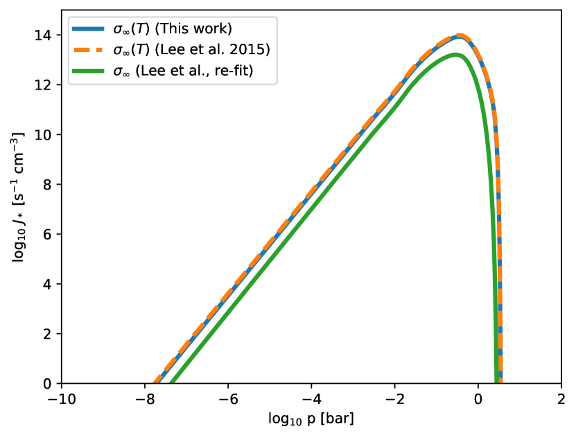
Figure 11: The classical nucleation rate for TiO₂ for three different surface tensions $\sigma_{\infty}$. The temperature - pressure profile is equivalent to the solid blue line in Figure 8. Top: The nucleation rate at different temperatures. Nucleation rates derived from updated cluster data are overall more efficient and extend to higher temperatures. Bottom: The position of the peak of the nucleation rate within the atmosphere is very similar for the three different surface tensions However, nucleation stays efficient up until slightly lower pressures for updated cluster data.

4.3.2 Non-classical nucleation theory

If detailed cluster data for all small sizes $N$ are available, the nucleation rate can be computed using individual cluster growth rates. The non-classical nucleation rate is:

$$\centering J_{*}^{-1}(T)=\sum^{N_{max}}_{N=1}\left(\frac{\tau_{gr}(N,T)}{f^{\circ}(N,T)}\right)\@add@centering$$ (15)

with $\tau_{gr}$ from Eq. 10 and $f^{\circ}(N)$ the number density of a cluster of size $N$. This can be computed from the partial pressure of the latter through:

$$\centering f^{\circ}(N)=\frac{p^{\circ}(N)}{kT}\@add@centering$$ (16)

Applying the law of mass action to a cluster of size $N$ gives its partial pressure as:

$$\centering p^{\circ}(N)=p^{{\circ\kern-2.93999pt-}}\left(\frac{p^{\circ}(1)}{p^{{\circ\kern-2.93999pt-}}}\right)^{N}\exp\left(-\frac{\Delta_{f}G^{\circ}(N)-N\Delta_{f}G^{\circ}(1)}{RT}\right)\@add@centering$$ (17)

with $p^{\circ}(1)$ the partial pressure of the monomer and the reference pressure $p^{\circ\kern-2.93999pt-}=1$bar. The results for the non-classical nucleation rates can be found in Figure 12.

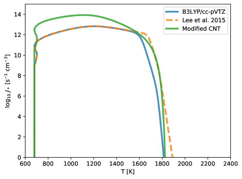
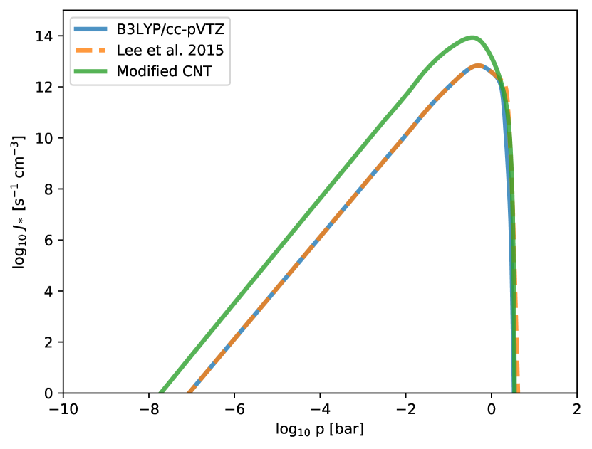
Figure 12: Nucleation rates $J_{*}$ for non-classical nucleation theory. The temperature - pressure profile is equivalent to the solid blue line in Figure 8. Using individual cluster data from this work (B3LYP/cc-pVTZ) (blue), cluster data from Lee et al. (2015) (orange dashed) and the modified CNT approach from section 4.3.1 (green). Top: Dependence on temperature. Bottom: Dependence on pressure.

4.4 Results for TiO₂ nucleation rates

For the modified classical nucleation approach, three values for the surface tension were compared. The shape of the nucleation rate in Fig. 11 is influenced by several factors. The reason for no nucleation occurring below a temperature of $T\approx 680$K is due to the p_gas, T_gas-profile used, which does not extend to lower temperatures (Fig. 8). On the upper temperature end, nucleation is limited due to its dependence on the supersaturation of the TiO₂ monomer. Because supersaturation ($S>1$) is required for nucleation and TiO₂ is no longer super-saturated at these high temperatures, no nucleation occurs. For lower temperatures, the surface tension from this work results in a higher nucleation rate than the recomputed surface tension with cluster data from for Lee et al. (2015) by $\sim$1 order of magnitude. The lower surface tension also leads to nucleation becoming inefficient at higher temperatures. Overall the value for the surface tension from this work agrees well with the value derived in Lee et al. (2015). However, using their cluster-data, we find a significantly higher surface tension (see Fig 11).

Nucleation rates for non-classical nucleation (Fig. 12) are lower than for MCNT for $T=680-1600$K by about 2 orders of magnitude. This is the result of taking into account individual cluster data for all sizes, instead of combining all the information into one quantity, the surface tension. Therefore, monomer growth processes from size $N$ to size $N+1$ are modelled more accurately. If one of the growth processes is less efficient than others it will bottleneck the overall nucleation rate. In this case $N+1$ is considered as the critical cluster size $N_{*}$. At higher temperatures ($T>1600$) cluster data from this work gives lower nucleation rates than both cluster data from Lee et al. (2015) and MCNT. There is no strict upper temperature limit for non-classical nucleation, as clusters can grow as long as it is energetically favorable for them to do and as long as nucleating material, i.e. TiO2 monomers, are available (Eq. 17). Since our updated cluster-data does predict nucleation of TiO₂ becoming inefficient at lower temperatures, the nucleation process starts at lower pressure levels, i.e. higher up in the model atmosphere.

5 Conclusion

This paper presents a method to find and optimise the geometries, zero-point energies, and thermochemical properties for clusters. Emphasis is put on exploring the parameter space of possible geometric configurations for these clusters as well as deriving their potential energies and thermochemical properties accurately. This approach was tested for small ($N=3-15$) (TiO₂)_N clusters. To ensure thermochemical accuracy, 129 combinations of DFT functionals and basis sets were tested with regards to their accuracy against known experimental data for the TiO₂ monomer. The B3LYP functional with the cc-pVTZ basis set and GD3BJ empirical dispersion was found to closely approach the experimental data and have been used for all final optimisation steps and frequency analysis. A new force field parameterisation of the Buckingham-Coulomb pair potential was presented, that more accurately reflects the cluster geometry (i.e. bond lengths) and energetic ordering for small TiO₂ clusters than previous parameterisations. For the DFTB description of interactions, the matsci set of Slater-Koster integrals was found to best reflect the energetic ordering for small clusters and their isomers given by the all-electron DFT calculations. The hierarchical optimisation approach works as intended and produces a large number of energetically low-lying isomers for all sizes. For the smallest clusters $N<7$, all global minimum candidates reported in the literature were found with methods that do not rely on using known cluster geometries. Since these are the same cluster sizes that are used to calibrate the less complex descriptions of inter-atomic potentials, this step of the approach is therefore independent of prior knowledge of cluster geometries. The Random approach of seed candidate creation is well suited to search small parameter spaces, such as $N<7$. However, for any cluster sizes $N>10$, the parameter space is too large to be searched with a fully randomised approach. For these larger cluster sizes the Mirror and Known+1 approaches produce the largest number of energetically low-lying isomers. However, they require prior knowledge of favourable clusters of size $N-1$ for Known+1 and of size $N/2$ for Mirror. This presents a constraint on the efficient search for clusters of these sizes, as without prior knowledge the global minima in potential energy will have to be found iteratively, always growing from $N$ to $N+1$. The current implementation of the hierarchical approach was able to find all known global minima for $N=3-11$, as well as a new global minimum candidate for $N=13$ that lies 6 kJ mol^-1 below the energy of the global minimum candidate structure reported by Lamiel-Garcia et al. (2017). For $N=12$ the global minimum known from the literature could not be reproduced, the closest isomer produced lies $2.45\frac{\mathrm{kJ}}{\mathrm{mol}}$ per monomer unit higher. For $N=14$ this energetic distance between the lowest found isomer and the known global minimum is $5.71\frac{\mathrm{kJ}}{\mathrm{mol}}$ per monomer unit and for $N=15$ it is $6.8\frac{\mathrm{kJ}}{\mathrm{mol}}$ per monomer unit. This shows that the search method is still incomplete for larger clusters. Since only clusters up to size $N=6$ had isomers that were used for calibration, the Mirror approach only had a single literature isomer to generate the clusters for $N=14$ and $N=15$, which drastically reduces the possible configurations explored by this approach.

To estimate the impact of the new thermochemical data on nucleation processes, the surface tension for small molecular clusters, as it is calculated in modified classical nucleation theory, was investigated. The findings of Lee et al. (2015) can not be reproduced, raising the best fit value for $\sigma_{\infty}$ for the test case at T$=1000$K to $\sigma_{\infty}=797$ erg cm^-2. The fast basis set def2svp gives $\sigma_{\infty}=325$ erg cm^-2, while the thermochemically more accurate basis set cc-pVTZ gives $\sigma_{\infty}=518$ erg cm^-2. The spread between these values is a factor of two, and as the surface tension appears in the exponent of the modified nucleation rate (Eq. 9) this spread is amplified. Since the B3LYP/cc-pVTZ functional/basis set was specifically chosen for its accuracy at modelling the thermochemical properties of small TiO₂ molecular clusters, the updated value for the surface tension represents the current best approximation. We find that for modified classical nucleation theory, the impact on the nucleation rates by the choice of the functional and basis set used to calculate the thermochemical properties is more important than finding a true global minimum, as long as the used structure is among the low-energy isomers. This is not true for non-classical nucleation description, which depends on accurate data for all sizes. The non-classical nucleation process described by the updated cluster data becomes inefficient at lower temperatures, putting the atmospheric lower border for seed formation through that process higher. A limitation of this description is that it only allows for homogeneous and homomolecular nucleation, ignoring pathways through cluster-cluster collisions and through species other than TiO₂.

We have shown that the updated cluster data has an impact on the nucleation rates both in their classical and non-classical description. Providing cluster data for larger clusters $N>15$ will allow a more detailed comparison with independent methods, for example with molecular dynamics methods as presented in Köhn et al. (2021). Additionally the spectroscopic properties of small (TiO₂)_N clusters, in particular the frequency-dependent opacities are interesting because they can allow for dust coagulation processes to be constrained through observations (Köhler et al., 2012). The methodology will be improved by additional candidate creation methods and applied to other potentially CCN-forming species in the atmospheres of hot Jupiters.

Appendix A Theoretical approaches used in this work

A.1 Density Functional Theory

Density functional theory can be used to describe the interactions between atoms and electrons within a molecule. The behaviour of every electron is influenced by every other electron in the system, leading to a system of highly coupled differential equations, whose dimensionality cannot be reduced and which has to be solved simultaneously. Therefore, numerical approximations are needed. The Hartree-Fock method (Hartree 1928) approximates the many-electron wavefunction as a product of single-electron wavefunctions. The single-electron wavefunctions are chosen, such that the many-body wavefunction built from them is anti-symmetric to obey the Pauli exclusion principle. The Hartree-Fock method is computationally still very expensive, because one equation has to be solved for every electron in the system. A computationally more efficient solution is given by density functional theory (DFT) (Hohenberg & Kohn 1964; Kohn & Sham 1965; Kohn et al. 1996). In DFT the multi-electron wavefunction is approximated by a function of the electron density. The electron density that minimises the total internal energy of a system is defined as its ground state. The interaction between electrons is then calculated through functionals of the electron density. The exact functionals are unknown. Many different approaches to describe and quantify these functionals have been investigated (Becke 2014). The first and simplest functionals use the local density approximation (LDA) (Hohenberg & Kohn 1964), where the functional is only dependent on the density at the exact coordinates where it is evaluated. This quickly leads to large inaccuracies as it assumes the homogeneity of the electron density, a variable that is highly non-homogeneous. More recent functionals use the gradient of the electron density as an additional qualifier. These functionals belong to the class of generalised gradient approximations (GGA)(Langreth & Mehl 1983). Most currently used functionals do not rely on pure DFT, but also have a component where the exchange energy is calculated from Hartree-Fock theory. These so-called hybrid functionals often combine high levels of accuracy with an acceptable computational cost, making them suitable for many purposes (Becke 1993a). In addition to choosing a functional, a basis set needs to be chosen for all DFT calculations. These basis sets represent a set of basis functions which can be combined linearly to express the electron orbitals in a computationally efficient way. These also exist at varying levels of complexity, mostly differing in the number of linear combinations that can be used to describe a single valence orbital. The choice of both the functional and basis set is crucial for the calculations in DFT. Section 2.3 is therefore dedicated to find the functional and basis set best suited for our purpose, which is the optimisation of (TiO₂)_$N$ clusters.

A.2 The Buckingham-Coulomb potential

The Buckingham-Coulomb potential takes into account the interatomic van der Waals forces, the Pauli exclusion principle and the electrostatic force, as opposed to the later used all-electron DFT calculations, which solve the Schrödinger equation to quantify the energy of a system. The general form of the Buckingham-Coulomb potential reads:

$$U(r_{ij})=A\ \mathrm{exp}\left(-\frac{r_{ij}}{B}\right)-\frac{C}{r_{ij}^{6}}+\frac{q_{i}q_{j}}{r_{ij}}$$ (18)

$U(r_{ij})$ is the potential energy of the interaction of two atoms $i$ and $j$, in this case O and Ti, O and O, or Ti and Ti. $r_{ij}$ is the distance between these atoms, and $q_{i}$ and $q_{j}$ are their respective charges. $A$, $B$, and $C$ are the Buckingham pair parameters. The first term in Eq. 18 represents the short-range repulsion according to the Pauli principle, with an increase in either parameter $A$ or $B$ leading to a increase in the potential barrier towards small distances. The second term describes the van der Waals force and its $r^{-6}$ dependency on inter-atomic distance. An increase in its parameter $C$ adds more attraction. The third and final term represents the Coulomb potential with its inverse proportionality to distance dominating the long-range interaction and implying alternating cation-anion ordering.

A.3 DFTB

In this work density functional based tight-binding methods are used as an intermediate step between a forcefield description and all-electron DFT calculations. The basis of DFTB models is expanding the total energy functional given by Kohn-Sham (KS) DFT (Kohn & Sham 1965) in a Taylor series of up to third order (Hourahine et al. 2020). There are several major approximations made in each term of the Taylor series. First order DFTB1 takes only the first order expansion into account. A valence-only minimal basis set is used with a linear combination of atomic orbitals (LCAO) ansatz. This means that only electrons in the outer shells of the individual atoms, the valence electrons, and their interactions are described by this model. Additionally a two-center approximation to the Hamiltonian operator is used, resulting in only interactions between neighboring electronic orbitals being taken into account, while distant overlapping orbitals are neglected. In this work, second order DFTB, also known as DFTB2 or SCC-DFTB (Self-consistent charge density functional tight-binding), is used. In addition to the first term of the Taylor series, in DFTB2 the second term also gets evaluated in order to calculate the energy of a system. Fluctuations in density, which become relevant in the second order term are approximated by a superposition of atomic contributions of all other atoms, each contributing an exponentially decaying spherically symmetric charge density.

Appendix B High level CCSD(T) calculations

Coupled cluster single point calculations at the CCSD(T)/6-311+G(2d,2p) level of theory have been run for the GM candidate clusters for $N$ = 1-4. (Tab. 7)

Table 7: Binding energies for GM candidate clusters for $N$=1-4 at the CCSD(T)/6-311+G(2d,2p) level of theory.

Size $N$	Ebind [$\frac{\mathrm{kJ}}{\mathrm{mol}}$]
1	1175.5
2	2844.1
3	4540.7
4	6163.8

The value for the monomer binding energy differs from the experimental Janaf Nist value by $\Delta E\approx 90\frac{\mathrm{kJ}}{\mathrm{mol}}$. This is far outside of both the assumed error of DFT and Janaf-Nist values of $\approx 4\frac{\mathrm{kJ}}{\mathrm{mol}}$. To calibrate our methods on these high-level theoretical calculations, we would therefore have to ignore the experimental values. To quantify how closely our chosen B3LYP/cc-pVTZ empdisp method matches the higher level results, the relative binding energies to the monomer were calculated for these clusters (Tab. 8).

Table 8: Relative binding energy to the monomer $\frac{E_{bind,N}}{E_{bind,1}}$

Size	CCSD(T)	DFT	Difference [%]
2	2.42	2.39	1.3
3	3.86	3.79	1.9
4	5.24	5.21	0.6

As the deviation is $<2\%$ for all sizes, we conclude that no information is lost by not using high-level CCSD(T) calculations to calibrate our methods.

Appendix C Calculating the Gibbs free energy of formation from the partition function

The Gibbs free energy of formation, $\Delta_{f}G^{\circ}$, for a gas-phase cluster can be calculated using its enthalpy of formation $\Delta_{f}H^{\circ}$, its entropy $S^{\circ}_{cluster}$, and the entropy of the individual atoms comprised in the cluster $S^{\circ}_{atoms}$:

$$\Delta_{f}G^{\circ}(T)=\Delta_{f}H^{\circ}(T)-T\left(S^{\circ}_{cluster}(T)-\sum S^{\circ}_{atoms}(T)\right)$$ (19)

For a cluster of size $N=5$, the last term is the sum of the entropies of 5 Ti atoms and 10 Oxygen atoms. Calculating the enthalpy of formation of the cluster requires information about the enthalpies of the elements that make up the cluster. The entropies and enthalpies for Ti and O used for these calculations are sourced from the JANAF-NIST tables (Malcolm W. Chase 1998). The enthalpy of formation of the cluster at temperature $T$ is then calculated through:

$$\Delta_{f}H^{\circ}(T)=\Delta_{f}H^{\circ}(T^{\circ\kern-2.93999pt-})+[H^{\circ}(T)-H^{\circ}(T^{\circ\kern-2.93999pt-})]_{cluster}\\ -\sum[H^{\circ}(T)-H^{\circ}(T^{\circ\kern-2.93999pt-})]_{atoms}$$ (20)

with the reference temperature $T^{\circ\kern-2.93999pt-}=0$K. The enthalpy of formation at the reference temperature $\Delta_{f}H^{\circ}(T^{\circ\kern-2.93999pt-})$ is the binding energy of the cluster, caluclated for a cluster of size $N$ through:

$$\Delta_{f}H^{\circ}(T^{\circ\kern-2.93999pt-})=E_{ZP}(\mathrm{Ti}_{N}\mathrm{O}_{2N})-NE_{ZP}({\rm Ti})-2NE_{ZP}({\rm O})$$ (21)

The entropy of the system $S^{\circ}_{cluster}$ is calculated from the internal energy of the system:

$$S^{\circ}_{cluster}=\frac{U(T)-U(0)}{T}+N_{atoms}k_{B}\left(\ln\frac{q(V,T)}{N_{atoms}}+1\right)$$ (22)

With the internal energy $U(T)-U(0)$, the partition function $q(V,T)$, and the number of atoms in the cluster $N_{atoms}$. The internal energy is derived from the partition function $q(V,T)$ through

$$U(T)-U(0)=-N_{atoms}\left(\frac{\partial\ln q(V,T)}{\partial\beta}\right)_{V}$$ (23)

Using the rigid-rotor harmonic-oscillator (RRHO) approximation for a polyatomic, non-linear molecule its partition function is:

$T$ is the temperature of the system, $\beta=\frac{1}{k_{B}T}$, with the Boltzmann constant $k_{B}$. $h$ is the Planck constant and $c$ the speed of light. $\sigma$ is the symmetry number, correcting for the repeated count of indistinguishable configurations. The unknown inputs in Eq. 24 are the vibrational levels $\nu_{i}$, the rotational constants A_rot, B_rot, and C_rot, and $V$, the volume of the particle, which are all outputs of the DFT simulations. For further reading on the calculation of these thermochemical properties, the reader is referred to Chapter 3.6 in Jeong (2000). The partition function used here omits the electronic partition function, $q_{el}$:

$$q_{el}=\sum_{i}g_{i}e^{-\beta\epsilon_{i}}$$ (25)

with the energy levels i, their energies $\epsilon_{i}$ and their respective degeneracies $g_{i}$. This is because Gaussian16 assumes that the first electronic excitation energy is much greater than the thermal energy ($\epsilon_{1}\gg kT$) and therefore inaccessible at any temperature, resulting in a value of $q_{el}=1$ for all cluster and temperatures. In addition, all clusters are assumed to be in a singlet state with g_i=1 $\forall$ i.

Appendix D Calibrations of low-level methods

D.1 Recalibrated force field

margin range destabilise the potential. Starting with a calculation of the potential energy of a (TiO₂)₅ cluster sourced from Berardo et al. (2014), the 10 individual parameters of the Buckingham-Coulomb force field parameterisation are varied until they destabilise the potential, so that it does not have a stable minimum. For each of the parameters the upper and lower value are taken as bounds for the following parameter search (See Table 9). The quality of a set of parameters is determined by a comparison with the energies and geometries calculated with DFT in Sect. 2.4.1. Due to the differences in approximation between the DFT and the force field calculations it is difficult to directly compare their respective results. Since force field calculations rely on a simplified representation of the PES, the absolute Buckingham pair binding energy of the clusters is not realistic when comparing to DFT calculations. However, the relative energies of isomers of the same size are portrayed accurately by the force field description and therefore used as a point of comparison. The monomer and dimer are not addressed with the force field approach, because of the impact of the electronic orbitals that is not considered in the Buckingham pair potential. For any uni-directional force field description the monomer and dimer have linear and flat geometries which are known to not be accurate (Koch & Manzhos 2017). For increasing cluster sizes, the interactions described by the force field grow stronger in comparison to the quantum effects and therefore give a more accurate description of the clusters. For each isomer from Sect. 2.4.1 a conp optimisation is performed using GULP. The energies of all isomers are then compared to the energy of the global minimum cluster of their respective size to determine their relative energy given by the force field approach $\Delta E_{ff}=E_{ff}^{min}-E_{ff}$. This difference in binding energy is then compared to the corresponding difference in binding energy from the DFT calculations $\Delta E_{DFT}=E_{DFT}^{min}-E_{DFT}$ for the same cluster. The quality of a parameter set with regards to the energy $Q(E)$ is then determined by the root sum squared of all relative deviations across all isomers (Eq. 26).

$$Q_{E}=\sqrt{\sum_{i}\left(\Delta E_{ff}(i)-\Delta E_{DFT}(i)\right)^{2}},\ \ i=\mathrm{isomers}$$ (26)

Additionally, the distance parameter $\bar{D}$ is introduced, which is calculated by taking the mean of all interatomic distances within a cluster. This is done to quantify the similarity of the geometries calculated by the force field approach and the DFT calculations. This distance parameter is calculated for every isomer, for both the DFT optimised geometry and the force field optimised geometry. The quality of a set of parameters with regards to the geometry $Q_{\mathrm{Geom}}$ is then calculated analogous to the energy quality by the root sum squared of all deviations of $\bar{D}_{ff}$ for the force field geometries from $\bar{D}_{DFT}$ for the DFT geometries.

$$Q_{\mathrm{Geom}}=\sqrt{\sum_{i}\left(\bar{D}_{ff}(i)-\bar{D}_{DFT}(i)\right)^{2}},\ \ i=\mathrm{isomers}$$ (27)

As optimisation for both quantities at the same time is crucial, a weight is introduced to normalise the values of $Q_{Geom}$ and $Q_{E}$. Evaluation of typical values for $Q_{Geom}$ and $Q_{E}$ reveals a difference of one order of magnitude, giving a weight of 10 as a reasonable counter. The overall quality $Q_{\mathrm{Tot}}$ of a parameter set is then given by the root sum squared of the energy quality $Q(E)$ and the geometry quality $Q_{\mathrm{Geom}}$ with a weight of 10:

$$Q_{\mathrm{Tot}}=\sqrt{10\cdot Q_{\mathrm{Geom}}^{2}+Q_{E}^{2}}$$ (28)

The quality parameter $Q_{\mathrm{Tot}}$ is minimised in order to find the set of parameters for the Buckingham - Coulomb potential that best reproduces the results from DFT calculations. The minimisation is done using the scipy.optimize.differential_evolution algorithm (Storn & Price 1997), with the bounds from Table 9 as well as the bounds derived from the parameters of Lamiel-Garcia et al. (2017). This algorithm was chosen due to its capability to find a global minimum for a multidimensional, non-linear function, its convergence properties and ease of parallelisation. Convergence is achieved after 415 iterations giving a minimum quality parameter of $Q_{\mathrm{Tot}}=4.66$ and results in the parameter set listed in Table 9. A comparison to the performance of this new parameter set can be found in Figure 13. In particular, results are plotted for the force field parameterisation by Lamiel-Garcia et al. (2017) in Figures 13(a) & 13(b), for the values from Matsui & Akaogi (1991) in Figures 13(c) & 13(d), and for the results from this work in Figures 13(e) & 13(f). On the left panel of these plots, the relative energies compared to the energy of the known global minimum geometry (which is set to zero), and their relative deviation are calculated with both the force field description of interactions and all-electron DFT. The positions of the global minimum isomers for all sizes $N$ overlap in the top right-hand corner of each graph. The position on the $x$-axis, which represents the relative energy described by DFT calculations is the same for all isomers of all sizes, representing the most realistic energetic ordering when going from right to left. Ideally, the relative energies calculated from the force field model reproduces the same energetic ordering on the $y$-axis, going from top to bottom, creating a linear function with a slope of 1. In order to aid visually, this line has been plotted in black. In the right panel of Figure 13 the same approach is followed for the average interatomic distance parameter $\bar{D}$. In an ideal case, the interatomic distances from the force field calculations match their DFT optimised counterparts and fall on the black line with slope 1. Significant deviations of individual clusters from that line can be explained by the fact that in some cases the force field approach produces a different local minimum geometry to the DFT approach from the same starting geometry. Finally, to make sure that the result is not a numerical artifact, the values for each parameter were rounded to the same accuracy as the parameters from literature and still outperform them for our purpose (Table 10).

Table 9: Upper and lower stable limits for each of the 10 individual parameters of the Buckingham-Coulomb force field (Eq. 18). These values are taken as upper and lower bounds for the parameter search.

Parameter	Lower	Upper	Final result
	bound	bound
ZTi	1.0	4.0	2.0122427
Ti-Ti A	25000	95000	79003.238832
Ti-Ti B	0.1	0.4	0.2221871
Ti-Ti C	100	850	475.3962942
O-O A	1000	25000	4164.7007783
O-O B	0.1	0.5	0.2836446
O-O C	5	250	19.7054331
Ti-O A	5000	80000	23420.6827084
Ti-O B	0.1	0.4	0.1759698
Ti-O C	0	20	4.5016462

Table 10: Comparison of Quality parameters $Q_{Tot}$, $Q_{Geom}$, and $Q_{E}$ for parameterisations from literature versus this work and this work rounded to the same precision as the literature.

Parameter source	$Q_{Tot}$	$Q_{Geom}$	$Q_{E}$
Lamiel-Garcia et al. (2017)	5.65	0.33	4.58
Matsui & Akaogi (1991)	11.35	0.86	7.47
This work	4.66	0.27	3.79
This work (rounded)	4.92	0.29	3.96

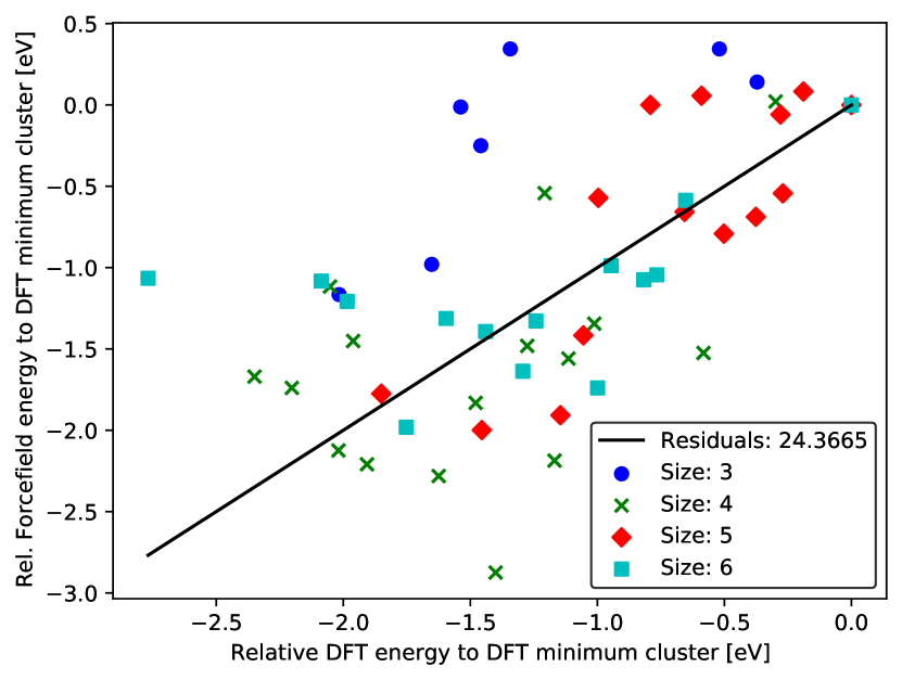
(a)

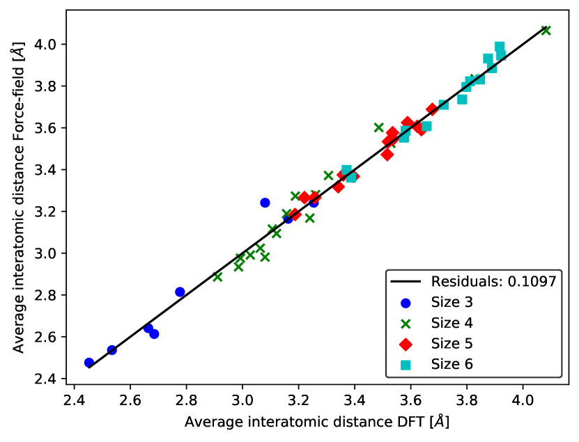
(b)

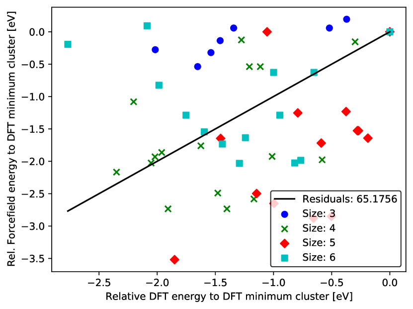
(c)

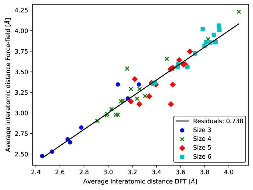
(d)

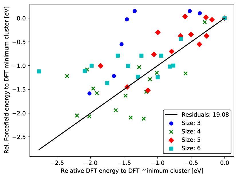
(e)

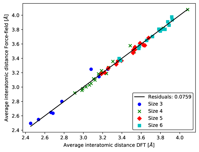
(f)

Figure 13: Left: Relative energy deviation to the global minimum cluster for the force field approach versus the DFT approach for all clusters from Section 2.4.1. Ideally, if the force field approach exactly reproduced the results of the more accurate DFT approach, all points would be on the black line with slope 1. Right: Distance parameter $\bar{D}$ for all clusters from the force field paramterisation versus the DFT approach. In an ideal scenario all clusters are exactly reproduced and therefore have no deviation from the black line with slope 1. Parameters from: Top: Lamiel-Garcia et al. (2017). Middle: Matsui & Akaogi (1991). Bottom: This work.

D.2 DFTB calibration

For the DFTB description of interactions, the energies and forces due to exchange-correlations between individual atoms are described by Slater-Koster integrals. These are constructed and pre-calculated for different purposes and collected in the form of Slater-Koster files on the website . In this work, all three available Slater-Koster files that describe the Titanium-Oxygen interaction are evaluated to determine which of these three integrals reproduces the results of the all-electron DFT calculations most accurately. In order to do this, the three Slater-Koster files, matsci (Luschtinetz et al. 2009), trans3d (Zheng et al. 2007), and tiorg (Dolgonos et al. 2010) are used to calculate the binding energies for all clusters from Sect. 2.4.1 according to Eq. 4. These calculated energies for all isomers of each size ($N=3,..,6$) are then compared to the energy of the global minimum isomer of that respective size to get a relative energy, equivalent to the approach for the force fields in Sect. D.1. These are again compared to the relative energies that result from the DFT calculations (Fig. 15). Analogous to the left panel in Fig. 13, the relative energy deviations to the global minimum are plotted for the DFT calculations. An ideal description matches ordering in both directions and falls onto a slope of 1 (black line). If any clusters fall above the horizontal $0$ eV line, the DFTB parametrisation shows a different isomer as the global minimum for this cluster size, which is not desirable. When comparing the plots in Figure 15, it becomes apparent that for trans3d (Fig. 15(a)) and tiorg (Fig. 15(b)) there are several isomers for all cluster sizes $N=3-6$ and $N=3,5$ respectively that fall above the horizontal $0$ eV line and therefore represent unlikely global minima candidates found by their DFTB description. For matsci (Fig. 14(a)), this is not the case and the lowest-energy isomer corresponds to the global minima candidate derived from all-electron DFT calculations for each respective cluster size. Visual inspection also shows that the deviation of individual isomers from the linear function with slope 1 is the smallest for matsci, telling that it reproduces the energetic ordering of the DFT calculations the best. In comparison, both trans3d and tiorg have large individual outliers for almost all cluster sizes. In order to quantify the quality of each of the Slater-Koster integral sets, the deviation of their relative energies as compared to the relative all-electron DFT energies is calculated. The sum of these residuals is equivalent to $Q_{E}$ in Sec. D.1 and is given in the plots. The visual inspection is confirmed, as the matsci set far outperforms the other two. Therefore the matsci set of Slater-Koster integrals, is used for all DFTB calculations in this work.

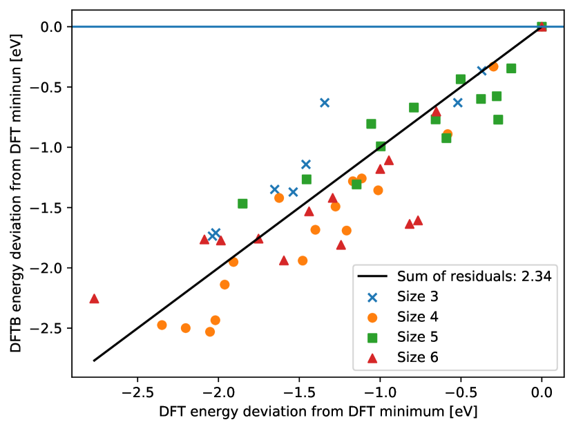
(a)

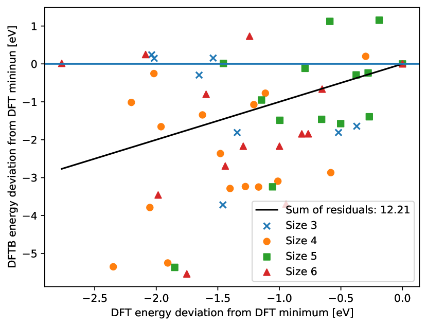
(a)

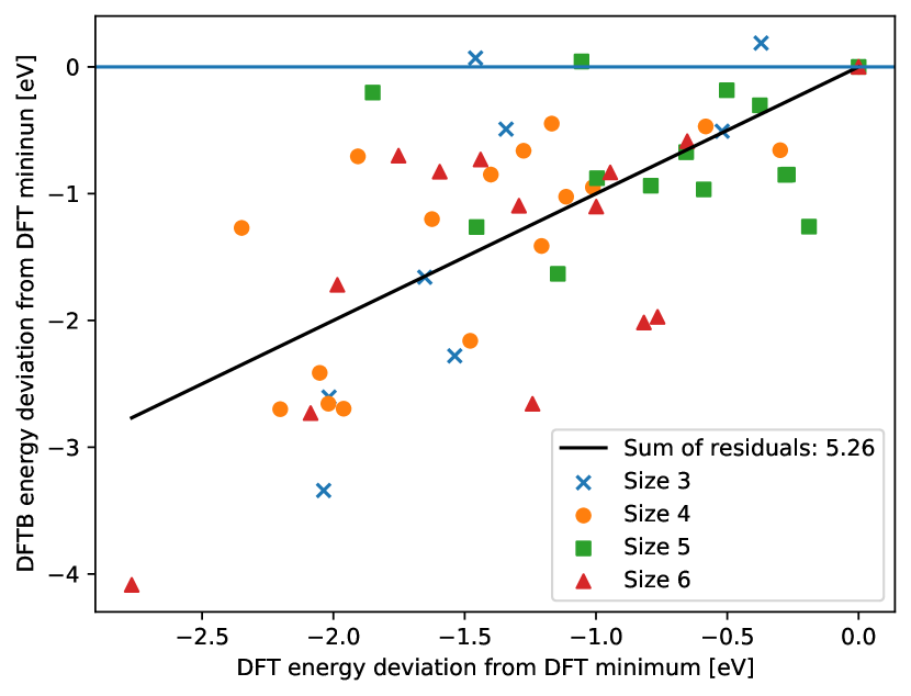
(b)

Figure 15: Comparison between DFT and DFTB energetic orderings for three different sets of Slater-Koster integrals. (a): Matsci Slater-Koster integrals. (b): Trans3d Slater-Koster integrals. (c): Tiorg Slater-Koster integrals. Positions of all isomers on the $x$-axis are consistent throughout all three figures. The energy level of the global minimum according to DFT is given by the blue horizontal lines. The relative energetic ordering from the DFT calculations is given by their order from right to left, whereas the DFTB ordering is given from top to bottom.