Start Small, Think Big:
On Hyperparameter Optimization
for Large-Scale Knowledge Graph Embeddings

Abstract

Knowledge graph embedding (KGE) models are an effective and popular approach to represent and reason with multi-relational data. Prior studies have shown that KGE models are sensitive to hyperparameter settings, however, and that suitable choices are dataset-dependent. In this paper, we explore hyperparameter optimization (HPO) for very large knowledge graphs, where the cost of evaluating individual hyperparameter configurations is excessive. Prior studies often avoided this cost by using various heuristics; e.g., by training on a subgraph or by using fewer epochs. We systematically discuss and evaluate the quality and cost savings of such heuristics and other low-cost approximation techniques. Based on our findings, we introduce GraSH, an efficient multi-fidelity HPO algorithm for large-scale KGEs that combines both graph and epoch reduction techniques and runs in multiple rounds of increasing fidelities. We conducted an experimental study and found that GraSH obtains state-of-the-art results on large graphs at a low cost (three complete training runs in total).

1 Introduction

A knowledge graph (KG) is a collection of facts describing relationships between a set of entities. Each fact can be represented as a (subject, relation, object)-triple such as (Rami Malek, starsIn, Mr. Robot). Knowledge graph embedding (KGE) models [4, 8, 16, 21, 23, 28] represent each entity and each relation of the KG with an embedding, i.e., a low-dimensional continuous representation. The embeddings are used to reason about or with the KG; e.g., to predict missing facts in an incomplete KG [15], for drug discovery in a biomedical KG [14], for question answering [18, 19], or visual relationship detection [2].

Prior studies have shown that embedding quality is highly sensitive to the hyperparameter choices used when training the KGE model [1, 17]. Moreover, the search space is large and hyperparameter choices are dataset- and model-dependent. For example, the best configuration found for one model may perform badly for a different one. As a consequence, we generally cannot transfer suitable hyperparameter configurations from one dataset to another or from one KGE model to another. Instead, a separate hyperparameter search is often necessary to achieve high-quality embeddings.

While using an extensive hyperparameter search may be feasible for smaller datasets—e.g., the study of Ruffinelli et al. [17] uses 200 configurations per dataset and model—, such an approach is generally not cost-efficient or even infeasible on large-scale KGs, where KGE training is expensive in terms of runtime, memory consumption, and storage cost. For example, the Freebase KG consists of $\approx 86\,\text{M}$ entities and more than $300\,\text{M}$ triples. A single training run of a 512-dimensional ComplEx embedding model on Freebase takes up to $50\,\text{min}$ per epoch utilizing 4 GPUs and requires $\approx 164\text{\,GB}$ of memory to store the model.

To reduce these excessive costs, prior studies on large-scale KGE models either avoid hyperparameter optimization (HPO) altogether or reduce runtime and memory consumption by employing various heuristics. The former approach leads to suboptimal quality, whereas the impact in terms of quality and cost of the heuristics used in the latter approach has not been studied in a principled way. The perhaps simplest of such heuristics is to evaluate a given hyperparameter configuration using only a small number of training epochs (e.g., [11] uses only 20 epochs for HPO on the Wikidata5M dataset). Another approach is to use a small subset of the large KG (e.g., the small FB15k benchmark dataset instead of full Freebase) to obtain a suitable hyperparameter configuration [11, 13, 30] or a set of candidate configurations [29]. The general idea behind these heuristics is to employ low-fidelity approximations (fewer epochs, smaller graph) to compare the performance of different hyperparameter configuration during HPO, before training the final model on full fidelity (many epochs, entire graph).

In this paper, we explore how to effectively use a given HPO budget to obtain a high-quality KGE model. To do so, we first summarize and analyze both cost and quality of various low-fidelity approximation techniques. We found that there are substantial differences between techniques and that a combination of reducing the number of training epochs and the graph size is generally preferable. To reduce KG size, we propose to use its $k$-core subgraphs [20]; this simple approach worked best throughout our study.

Building upon these results, we present GraSH, an efficient HPO algorithm for large-scale KGE models. At its heart, GraSH is based on successive halving [10]. It uses multiple fidelities and employs several KGE-specific techniques, most notably, a simple cost model, negative sample scaling, subgraph validation, and a careful choice of fidelities. We conducted an extensive experimental study and found that GraSH achieved state-of-the-art results on large-scale KGs with a low overall search budget corresponding to only three complete training runs. Moreover, both the use of multiple reduction techniques simultaneously and of multiple fidelity levels was key for reaching high quality and low resource consumption.

2 Preliminaries and Related Work

A general discussion of KGE models and training is given in [15, 25]. Here we summarize key points and briefly discuss prior approaches to HPO.

Knowledge graph embeddings. A knowledge graph $\mathcal{G}=(\mathcal{E},\mathcal{R},\mathcal{K})$ consists of a set $\mathcal{E}$ of entities, a set $\mathcal{R}$ of relations, and a set $\mathcal{K}\subseteq\mathcal{E}\times\mathcal{R}\times\mathcal{E}$ of triples. Knowledge graph embedding models [4, 8, 16, 21, 23, 28] represent each entity $i\in\mathcal{E}$ and each relation $p\in\mathcal{R}$ with an embedding ${\boldsymbol{e}}_{i}\in\mathbb{R}^{d}$ and ${\boldsymbol{e}}_{p}\in\mathbb{R}^{d}$, respectively. They model the plausibility of each subject-predicate-object triple $(s,p,o)$ via a model-specific scoring function $f({\boldsymbol{e}}_{s},{\boldsymbol{e}}_{p},{\boldsymbol{e}}_{o})$, where high scores correspond to more, low scores to less plausible triples.

Training and training cost. KGE models are trained [25] to provide high scores for the positive triples in $\mathcal{K}$ and low scores for negative triples by minimizing a loss such as cross-entropy loss. Since negatives are typically unavailable, KGE training methods employ negative sampling to generate pseudo-negative triples, i.e., triples that are likely but not guaranteed to be actual negatives. The number $N^{-}$ of generated pseudo-negatives per positive is an important hyperparameter influencing both model quality and training cost. In particular, during each epoch of training a KGE model, all positives and their associated negatives are scored, i.e., the overall number of per-epoch score computations is $(\lvert\mathcal{K}\rvert+1)N^{-}$. We use this number as a proxy for computational cost throughout. The size of the KGE model itself scales linearly with the number of entities and relations, i.e., $O(\lvert\mathcal{E}\rvert d+\lvert\mathcal{R}\rvert d)$ if all embeddings are $d$-dimensional.

Evaluation and evaluation cost. The standard approach to evaluate KGE model quality for link prediction task is to use the entity ranking protocol and a filtered metric such as mean reciprocal rank (MRR). For each $(s,p,o)$-triple in a held-out test set $\mathcal{K}^{\text{test}}$, this protocol requires to score all triples of form $(s,p,?)$ and $(?,p,o)$ using all entities in $\mathcal{E}$. Overall, $\lvert\mathcal{K}^{\text{test}}\rvert\lvert\mathcal{E}\rvert$ scores are computed so that evaluation cost scales linearly with the number of entities. Since this cost can be substantial, sampling-based approximations have been used in some prior studies [13, 30]. We do not use such approximations here since they can be misleading in that they do not reflect model quality faithfully [11].

Hyperparameters. The hyperparameter space for KGE models is discussed in detail in [1, 17]. Important hyperparameters include embedding dimensionalities, training type, number $N^{-}$ of negatives, sampling type, loss function, optimizer, learning rate, type and weight of regularization, and amount of dropout.

Full-fidelity HPO. Recent studies analyzed the impact of hyperparameters and training techniques for KGE models using full-fidelity HPO [1, 17]. In these studies, the vast hyperparameter search space was explored using a random search and Bayesian optimization with more than $200$ full training runs per model and dataset. The studies focus on smaller benchmark KGs, however; such an approach is excessive for large-scale knowledge graphs.

Low-fidelity HPO. Current work on large-scale KGE models circumvented the high cost of full-fidelity HPO by relying on low-fidelity approximations such as epoch reduction [5, 11] and using smaller benchmark graphs [11, 13, 30] in a heuristic fashion. The best performing hyperparameters in low-cost approximations were directly applied to train a single full-fidelity model. Our experimental study suggests that such an approach may neither be cost-efficient nor produce high-quality results.

Two-stage HPO. AutoNE [24] is an HPO approach for training large-scale network embeddings that optimizes hyperparameters in two stages. It first approximates hyperparameter performance on subgraphs created by random walks, a technique that we will explore in Sec. 4. Subsequently, AutoNE transfers these results to the full graph using a meta learner. In the context of KGs, this approach was outperformed by KGTuner [29], which uses a multi-start random walk (fixed to $20\%$ of the entities) in the first stage and evaluates the top-performing configurations (fixed to $10$) at full fidelity in the second stage. Such fixed heuristics often limit flexibility in terms of budget allocation and lead to an expensive second stage on large KGs. In contrast, GraSH makes use of multiple fidelity levels, carefully constructs and evaluates low-fidelity approximations, and adheres to a prespecified overall search budget. These properties are key for large KGs; see Sec. 5.3 for an experimental comparison with KGTuner.

3 Successive Halving for Knowledge Graphs (GraSH)

GraSH is a multi-fidelity HPO algorithm for KGE models based on successive halving [10]. As successive halving, GraSH proceeds in multiple rounds of increasing fidelity; only the best configurations from each round are transferred to the next round. In contrast to the HPO techniques discussed before, this approach allows to discard unpromising configurations at very low cost. GraSH differs from successive halving mainly in its parameterization and its use of KG-specific reduction and validation techniques.

Parameterization. GraSH is summarized as Alg. 1. Given knowledge graph $\mathcal{G}$, GraSH outputs a single optimized hyperparameter configuration. GraSH is parameterized as described in Alg. 1; default parameter values are given in parentheses if applicable. The most important parameters are the maximal number $E$ of epochs and the overall search budget $B$. The search budget $B$ is relative to the cost of a full training run, which in turn is determined by $E$. The default choice $B=3$, for example, corresponds to an overall search cost of three full training runs. We chose this parameterization because it is independent of utilized hardware and both intuitive and well-controllable. The reduction factor $\eta$ controls the number of configurations (starts at $n$, decreases by factor of $\eta$ per round) and fidelity (increases by factor of $\eta$) of each round. Note that GraSH does not train at full fidelity, i.e., its final configuration still needs to be trained on the full KG (not part of budget $B$). Finally, GraSH is parameterized by a variant $v$. This parameter controls which reduction technique to use (only epoch, only graph, or combined).

Algorithm 1 GraSH: Successive Halving for Knowledge Graph Embeddings

KG $\mathcal{G}=(\mathcal{E},\mathcal{R},\mathcal{K})$, max. epochs $E$, search budget $B$ (=3), num. configurations $n$ (=64), reduction factor $\eta$ (=4), variant $v\in\{$epoch, graph, combined$\}$ (=combined)

Hyperparameter configuration

1:$s\leftarrow\lceil\log_{\eta}(n)\rceil$ $\triangleright$ Number of rounds

2:$R\leftarrow B/s$ $\triangleright$ Per-round budget

3:$\Lambda_{1}\leftarrow\{\lambda_{1},...,\lambda_{n}\}$ $\triangleright$ Generate $n$ hyperparameter configurations

4:for $i\in\{1,...,s\}$ do $\triangleright$ $i$-th round

5:     $f_{i}\leftarrow R/|\Lambda_{i}|$ if $v\neq\textit{combined}$ else $R/\sqrt{|\Lambda_{i}|}$$\triangleright$ Target fidelity

6:     $E_{i}\leftarrow f_{i}E$ if $v\neq$ graph else $E$ $\triangleright$ Epochs in round $i$

7:     $\mathcal{G}_{i}\leftarrow$ reduced KG with $f_{i}|\mathcal{K}|$ triples if $v\neq$ epoch else $\mathcal{G}$ $\triangleright$ Graph in round $i$

8:     $\mathcal{G}_{i}^{\text{train}},\mathcal{G}_{i}^{\text{valid}}\leftarrow$ random train-valid split of $\mathcal{G}_{i}$

9:     $V_{i}\leftarrow$ train each $\lambda\in\Lambda_{i}$ on $\mathcal{G}_{i}^{\text{train}}$ for $E_{i}$ epochs and validate using $\mathcal{G}_{i}^{\text{valid}}$

10:     $\Lambda_{i+1}\leftarrow$ best $\lceil|\Lambda_{i}|/\eta\rceil$ configurations from $\Lambda_{i}$ according to $V_{i}$

11:end for

12:return $\Lambda_{s+1}$ $\triangleright$ Only single configuration left

Algorithm overview. Like successive halving, GraSH proceeds in rounds. Each round has approximately the same overall budget, but differs in the number of configurations and fidelity. For example, using the default settings of $B=3$, $n=64$ and $\eta=4$, GraSH uses three rounds with 64, 16, and 4 configurations and a fidelity of 1/64, 1/16, 1/4, respectively. The hyperparameter configurations in the first round are sampled randomly from the hyperparameter space. Depending on the variant being used, GraSH reduces the number of epochs, the graph size, or both to reach the desired fidelity. If no reduced graph corresponds to the fidelity, the next smaller one is used. After validating each configuration (see below), the best performing $1/\eta$-th of the configurations is passed on to the next round. This process is repeated until only one configuration remains.

Validation on subgraphs. Care must be taken when validating a KGE model trained on a subgraph, e.g., $\mathcal{G}_{i}=(\mathcal{E}_{i},\mathcal{R}_{i},\mathcal{K}_{i})$ in round $i$. Since $\mathcal{G}_{i}$ typically contains a reduced set of entities $\mathcal{E}_{i}\subseteq\mathcal{E}$, a full validation set for $\mathcal{G}$ cannot be used. This is because no embedding is learned for the “unseen” entities in $\mathcal{E}\setminus\mathcal{E}_{i}$, so that we cannot score any triples containing these entities (as required by the entity ranking protocol). To avoid this problem, we explicitly create new train and valid splits $\mathcal{G}_{i}^{\text{train}}$ and $\mathcal{G}_{i}^{\text{valid}}$ in round $i$. Here, $\mathcal{K}_{i}^{\text{valid}}$ is sampled randomly from $\mathcal{K}_{i}$ and $\mathcal{K}_{i}^{\text{train}}=\mathcal{K}_{i}\setminus\mathcal{K}_{i}^{\text{valid}}$. Although this approach is very simple, it worked well in our study. An alternative is the construction of “hard” validation sets as in [22]. We leave the exploration of such techniques to future work.

Negative sample scaling. Recall that the number $N^{-}$ of negative samples is an important hyperparameter for KGE model training. Generally (and assuming without-replacement sampling), each entity is sampled as a negative with probability $N^{-}/\lvert\mathcal{E}\rvert$. When we use a subgraph $\mathcal{G}_{i}$ as in GraSH, this probability increases to $N^{-}/\lvert\mathcal{E}_{i}\rvert$, i.e., each entity is more likely to act as a negative sample due to the reduction of the number of entities. To correctly assess hyperparameter configurations in such cases, GraSH scales the number of negative examples and uses $N^{-}_{i}=\frac{\lvert\mathcal{E}_{i}\rvert}{\lvert\mathcal{E}\rvert}N^{-}$ in round $i$. This choice preserves the probability of sampling each entity as a negative and provides additional cost savings since the total number of scored triples is further reduced in low-fidelity experiments.

Cost model and budget allocation. To distribute the search budget $B$ over the rounds, we make use of a simple cost model to estimate the relative runtime of low-fidelity approximations. This cost model drives the choice of $f_{i}$ in Alg. 1. In particular, we assume that training cost is linear in both the number of epochs ($E_{i}$) and the number of triples ($\lvert\mathcal{K}_{i}\rvert$). For example, this implies that training five configurations for one epoch has the same cost as training one configuration for five epochs. Likewise, training five configurations with 20% of the triples has the same cost as training one configuration on the whole KG. Using this assumption, the relative cost of evaluating a single hyperparameter configuration in round $i$ is given by $\frac{E_{i}}{E}\frac{\lvert\mathcal{K}_{i}\rvert}{\lvert\mathcal{K}\rvert}$. More elaborate cost models are conceivable, but this simple approach already worked well in our experimental study. Note, for example, that our simple cost model neglects negative sample scaling and thus tends to overestimate (but avoids underestimation) of training cost.

4 Low-fidelity Approximation Techniques

In this section, we summarize and discuss various low-fidelity approximation techniques. As discussed previously, the two most common types are graph reduction (i.e. training on a reduced graph) and epoch reduction (i.e., training for fewer epochs). Note that although graph reduction is related to dataset reduction techniques used in other machine learning domains, it represents a major challenge since the relationships between entities need to be taken into account.

Generally, good low-fidelity approximations satisfy the following criteria:

1. Low cost. Computational and memory costs for model training (including model initialization) and evaluation should be low. Recall that computational costs are mainly determined by the number of triples, whereas memory and evaluation cost are determined by the number of entities. Ideally, both quantities are reduced.

2. High transferability. Low-fidelity approximations should transfer to the full KG in that they provide useful information. E.g., rankings of low-fidelity approximations should match or correlate with the rankings at full-fidelity.

3. Flexibility. It should be possible to flexibly trade-off computational cost and transferability.

All three points are essential for cost-effective and practical multi-fidelity HPO.

In the following, we present the graph reduction approaches triple sampling, multi-start random walk, and $k$-core decomposition, as well as epoch reduction. A high-level comparison of these approaches w.r.t. the above desiderata is provided in Tab. 1. The assessment given in the table is based on our experimental results (Sec. 5.2).

Table 1: Comparison of low-fidelity approximation techniques.

Technique	Low Cost	High Transferability	Flexibility
Triple sampling	$\circ$	-	+
Random walk	$\circ$	$\circ$	+
$k$-core decomposition	+	+	$\circ$
Epoch reduction	-	$\circ$	+

4.1 Graph Reduction

Graph reduction techniques produce a reduced KG $\mathcal{G}_{i}=(\mathcal{E}_{i},\mathcal{R}_{i},\mathcal{K}_{i})$ from the full KG $\mathcal{G}=(\mathcal{E},\mathcal{R},\mathcal{K})$. This is commonly done by first determining the reduced set $\mathcal{K}_{i}$ of triples and subsequently retaining only those entities (in $\mathcal{E}_{i}$) and relations (in $\mathcal{R}_{i}$) that occur in $\mathcal{K}_{i}$. A reduction in triples thus may lead to a reduction in the number of entities and relations as well. This consequently results in further savings in computational cost, evaluation cost, and memory consumption. The graph reduction techniques discussed here are illustrated in Fig. 1.

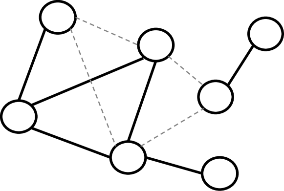
(a) Triple sampling
(60%).

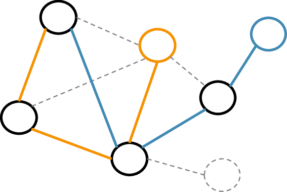
(b) Random walk
($s=2$, $l=3$).

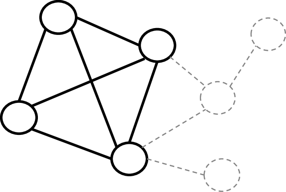
(c) $k$-core decomposition
($k=3$).

Figure 1: Schematic illustration of selected graph reduction techniques. All reduced graphs contain 6 of the 10 original triples but a varying number of entities.

Triple sampling (Fig. 1(a)). The perhaps simplest approach to reduce graph size is to sample triples randomly from the graph. As shown in Fig. 1(a), many entities with sparse interconnections can remain in the resulting subgraphs (e.g., the two entities at the top right) so that $\mathcal{E}_{i}$ tends to be large. The cost in terms of model size and evaluation time is consequently only slightly reduced. We also observed (see Sec. 5.2) that triple sampling leads to low transferability, most likely due to this sparsity. Triple sampling does offer very good flexibility, however, since triple sets of any size can be constructed easily.

Random walk (Fig. 1(b)). In multi-start random walk, which is used in AutoNE [24], a set of $s$ random entities is samples from $\mathcal{E}$. A random walk of length $l$ is started from each of these entities and the resulting triples form $\mathcal{K}_{i}$. Empirically, many entities may ultimately remain so that the reduction of memory consumption and evaluation cost is limited. Although the resulting subgraph tends to be better connected than the ones obtained by triple sampling, transferability is still low and close to triple sampling (again, see Sec. 5.2). As triple sampling, the approach is very flexible though. KGTuner [29] improves on the basic random walk considered here by using biased starts and adding all connections between the retained entities (even if they do not occur in a walk). The $k$-core decomposition, which we discuss next, offers a more direct approach to obtain such a highly-connected graph.

$k$-core decomposition (Fig. 1(c)). The $k$-core decomposition [20] allows for the construction of subgraphs with increasing cohesion. The $k$-core subgraph of $\mathcal{K}$, where $k\in\mathbb{N}$ is a parameter, is defined as the largest induced subgraph in which every retained entity (i.e., $\mathcal{E}_{i}$) occurs in at least $k$ retained triples (i.e., in $\mathcal{K}_{i}$). The computation of $k$-cores is cheap and supported by common graph libraries. Generally, $k$-cores contain only a small number of entities because long-tail entities with infrequent connections are removed. Moreover, they are highly interconnected by construction. As a consequence, we found that computational cost and memory consumption is low and transferability high. The approach is less flexible than the other graph reduction techniques, as the choice of $k$ and the graph structure determines the resulting fidelity. One may interpolate between $k$-cores for improved flexibility but we do not explore this approach in this work.

4.2 Epoch Reduction

Epoch reduction is the most common form of fidelity control used in HPO [3, 26]. As the set $\mathcal{E}$ of entities does not change with varying fidelity, memory and evaluation cost are very large even when using low-fidelity approximations. We observed good transferability as long as the number of epochs is not too small (Sec. 5.2); otherwise, transferability is often considerably worse than graph reduction techniques. This limits flexibility: Especially on large-scale graphs, the overall training budget often consists of only a small number of epochs in the first place (e.g., $10$ as in [11, 30]). Note that the available budget in low-fidelity approximations can be smaller than the cost of one complete epoch (when $f_{i}<1/E$ in Alg. 1). Although partial epochs can be used easily, epoch reduction then corresponds to a form of triple sampling (with the additional disadvantage of not reducing the set of entities).

4.3 Summary

In summary, as long the desired fidelity is sufficiently high, epoch reduction offers high-quality approximations and high flexibility. It does not improve memory consumption and evaluation cost, however, and it leads to high cost and low quality on large-scale graphs with limited budget. Graph reduction approaches, on the other hand, reduce the number of entities and hence memory consumption and evaluation cost. Compared to triple sampling and random walks, the $k$-core decomposition has the highest transferability and lowest cost. In GraSH, we use a combination of epoch reduction and $k$-core decomposition by default to avoid training for partial epochs and the use of very small subgraphs with low-fidelity.

5 Experimental Study

We conducted an experimental study to investigate (i) to what extent hyperparameter rankings obtained with low-fidelity approximations correlate with the ones obtained at full fidelity (Sec. 5.2); (ii) the performance of GraSH in terms of quality (Sec. 5.3), resource consumption (Sec. 5.4) and robustness (Sec. 5.5). In summary, we found that:

1. GraSH was cost-effective and produced high-quality hyperparameter configurations. It reached state-of-the-art results on a large-scale graph with a small overall search budget of three complete training runs (Sec. 5.3).

2. Using multiple reduction techniques was beneficial. In particular, a combination of graph- and epoch-reduction performed best (Sec. 5.2 and 5.3).

3. Low-fidelity approximations correlated best to full fidelity for graph reduction using the $k$-core decomposition and, as long as the budget was sufficiently large, second-best for epoch reduction (Sec. 5.2).

4. Graph reduction was more effective than epoch reduction in terms of reducing computational and memory cost. Evaluation using small subgraphs had low memory consumption and short runtimes (Sec. 5.4).

5. Using multiple rounds with increasing fidelity levels was beneficial (Sec. 5.5).

6. GraSH was robust to changes in budget allocation across rounds (Sec. 5.5).

Table 2: Dataset statistics.

Scale	Dataset	Entities	Relations	$|$Train$|$	$|$Valid$|$	$|$Test$|$
Small	Yago3-10	123 182	37	1 079 040	5 000	5 000
Medium	Wikidata5M	4 594 485	822	21 343 681	5 357	5 321
Large	Freebase	86 054 151	14 824	304 727 650	1 000	10 000

5.1 Experimental Setup

Source code, search configurations, resulting hyperparameters, and an online appendix can be found at https://github.com/uma-pi1/GraSH.

Datasets. We used common KG benchmark datasets of varying sizes with a focus on larger datasets; see Tab. 2. Yago3-10 [8] is a subset of Yago 3 containing only entities that occur at least ten times in the complete graph. Wikidata5M [27] is a large-scale benchmark and the induced graph of the five million most-frequent entities of Wikidata. The largest dataset is Freebase as used in [11, 30]. For all datasets except Freebase, we use the validation and test sets that accompany the datasets to evaluate the final model. For Freebase, we used the sub-sampled validation (1 000 triples) and test sets (10 000 triples) from [11].

Hardware. All runtime, GPU memory, and model size measurements were taken on the same machine (40 Intel Xeon E5-2640 v4 CPUs @ 2.4GHz; 4 NVIDIA GeForce RTX 2080 Ti GPUs).

Implementation and models. GraSH uses DistKGE [11] for parallel training of large-scale graphs and HpBandSter [9] for the implementation of SH. We considered the models ComplEx [23], RotatE [21] and TransE [4]. ComplEx and RotatE are among the currently best-performing KGE models [1, 12, 17, 21] and represent semantic matching and translational distance models, respectively. All three models are commonly used for large-scale KGEs [11, 13, 30].

Hyperparameters. We used the hyperparameter search space of [11]. The search space consists of nine continuous and two categorical hyperparameters. The upper bound on the number of negative samples for ComplEx is 10 000 and for RotatE and TransE 1 000 (since these models are more memory-hungry). We set the maximum training epochs on Yago3-10 to $400$, on Wikidata5M to $64$, and on Freebase to $10$.

Methodology. For the GraSH search, we used the default settings ($B=3$, $\eta=4$, $n=64$). Apart from the upper bound of negatives, we used the same $64$ initial hyperparameter settings for all models and datasets to allow for a fair comparison. For graph reduction, we used $k$-core decomposition unless mentioned otherwise. Subgraph validation sets generated by GraSH consisted of 5 000 triples. The resulting best configurations are published along with our online appendix.

Metrics. We used the common filtered MRR metric to evaluate KGE model quality on the link prediction task as described in Sec. 2. Results for Hits@$k$ are given in our online appendix.

5.2 Comparison of Low-Fidelity Approximation Techniques (Fig. 2)

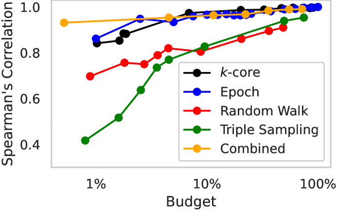
(a) Yago3-10 (max. $40$ epochs).

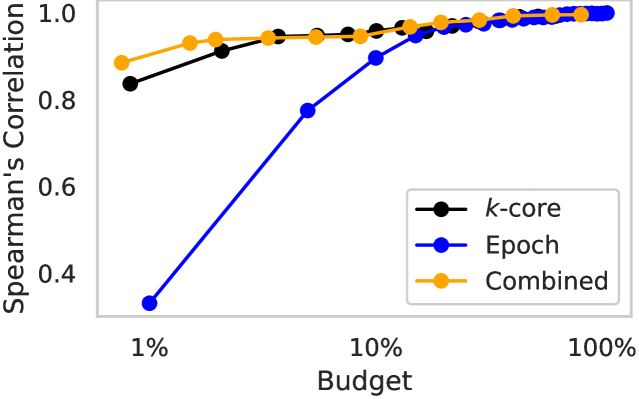
(b) Wikidata5M (max. $20$ epochs).

Figure 2: Comparison of low-fidelity approximations techniques. Shows Spearman’s rank correlation between low-fidelity approximations and a full-fidelity baseline. Budget (log-scale) corresponds to the relative amount of epochs and/or triples.

In our first experiment, we studied and compared the transferability of low-fidelity approximations to full-fidelity results. To do so, we first ran a full-fidelity hyperparameter search consisting of 30 pseudo-randomly generated trials. We then trained and evaluated the same 30 trials using the approximation techniques described in Sec. 4 at various budgets. To keep computational cost feasible, this experiment was only performed on the two smaller datasets and with a smaller number of epochs.

Since the validation sets used with graph reductions differ from the one used at full fidelity (see Sec. 3), we compared the ranking of hyperparameter configurations instead of their MRR metrics. In particular, we used Spearman’s rank correlation coefficient [31] between the low-fidelity and the high-fidelity results. A higher value corresponds to a better correlation.

Our results on Yago3-10 are visualized in Fig. 2(a). We found high transferability for the $k$-core decomposition and epoch reduction. Graph reduction based on triple sampling and random walks led to clearly inferior results and was not further considered. A combination of $k$-core subgraphs and reduced epochs (each contributing $50$% to the savings) further improved low-budget results.

To investigate the behavior on a larger graph, we evaluated the three best techniques on Wikidata5M, see Fig. 2(b). Recall that due to the high cost, a small number of epochs is often used for training on large KGs. This has a detrimental effect on the transferability of epoch reduction, as partial epochs need to be used for low-fidelity approximations (see Sec. 4.2). In particular, there is a considerable drop in transferability for epoch reduction below the 10% budget. This drop in performance is neither visible for the $k$-core approximations nor for the combined approach.

Note that even for the best low-fidelity approximation, the rank correlation increased with budget. This suggests that using multiple fidelities (as in GraSH) instead of a single fidelity is beneficial. In our study, this was indeed the case (see Sec. 5.5).

5.3 Final Model Quality (Tab. 3(b))

In our next experiment, we analyzed the performance of GraSH in terms of the quality of its selected hyperparameter configuration. Tab. 3(a) shows the test-data performance of this resulting configuration trained at full fidelity. We report results for different datasets, different reduction techniques, different KGE models, and different model dimensionalities.

Results (Tab. 3(a)). The combined variant of GraSH offered best or close to best results across all datasets and models. In comparison to the other variants, it avoided the drawbacks of training partial epochs (e.g., epoch reduction on Freebase) as well as using subgraphs that are too small (e.g., graph reduction on Yago3-10).

Comparison to prior results (Tab. 3(b)). We compared the results obtained by GraSH to the best published prior results known to us, see Tab. 3(b). Note that prior models were often trained at substantially higher cost. For example, on Wikidata5M, GraSH used an overall budget of $4\cdot 64=256$ epochs for HPO and training, whereas some prior methods used 1 000 epochs for a single training run. Likewise, dimensionalities of up to 1 000 were sometimes used. For a slightly more informative comparison, we performed a GraSH search with an increased dimensionality of $512$, but kept the low search and training budgets. Even with this low budget, we found that on small to midsize graphs, GraSH performed either similarly (ComplEx, Yago3-10 & Wikidata5M) and sometimes slightly worse (RotatE, Wikidata5M) than the best prior results. On the large-scale Freebase KG, where low-fidelity hyperparameter search is a necessity, GraSH outperformed state-of-the-art results by a large margin.

Table 3: Model quality in terms of MRR. State-of-the-art results underlined. Best reduction variant in bold. Note that best prior results often use a considerably larger budget and/or model dimensionality.

(a) GraSH with default settings ($B=3$, $n=64$, $\eta=4$).

	Dataset	Variant $\to$ Model $\downarrow$	Epoch Dim 128	Graph Dim 128	Comb. Dim 128	Comb. Dim 512
Small	Yago 3-10	ComplEx	0.536	0.463	0.528	0.552
		RotatE	0.432	0.432	0.434	0.453
	($E=400$)	TransE	0.499	0.422	0.499	0.496
Medium	Wiki- data5M	ComplEx	0.300	0.300	0.300	0.294
		RotatE	0.241	0.232	0.241	0.261
	($E=64$)	TransE	0.263	0.263	0.268	0.249
Large	Free- base	ComplEx	0.572	0.594	0.594	0.678
		RotatE	0.561	0.613	0.613	0.615
	($E=10$)	TransE	0.261	0.553	0.553	0.559

(b) Prior results

MRR	Dim	Epochs
0.551	128	400	[5]
0.495	1 000	?	[21]
0.510	350	4 000	[6]
0.308	128	300	[11]
0.290	512	1 000	[27]
0.253	512	1 000	[27]
0.612	400	10	[11]
0.567	128	10	[11]
-	-	-

Comparison to KGTuner. KGTuner [29] was developed in parallel to this work and follows similar goals as GraSH. We compared the two approaches on the smaller Yago3-10 KGE with ComplEx; a comparison on the larger datasets was not feasible since KGTuner has large computational costs. We ran both GraSH and KGTuner with the default settings of KGTuner ($n=50$ trials, $E=50$ epochs, dim. 1 000) to obtain a fair comparison. KGTuner reached an MRR of $0.505$ in about 5 days (its search budget corresponds to $B\approx 20$). GraSH reached an MRR of $0.530$ in about $1.5$ hours ($B=3$, sequential search on 1 GPU), i.e., a higher quality result at lower cost. The high computational cost of KGTuner mainly stems from its inflexible and inefficient budget allocation (e.g., always 10 full-fidelity evaluations). The higher quality of GraSH stems from its use of multiple fidelities (vs. two in KGTuner) and by using a combination of $k$-cores and epoch reduction (vs. random walks in KGTuner).

5.4 Resource Consumption (Tab. 4)

Table 4: Resource consumption per round (ComplEx).

		Round Time (min)			Model Size (MB)
		Epoch	Graph	Comb.	Epoch	Graph	Comb.
Yago3-10	Round 1	43.9	24.7	15.9	60.2	0.3	2.0
	Round 2	34.8	13.3	27.1	60.2	0.4	6.3
	Round 3	38.7	28.1	33.5	60.2	6.3	16.7
	Total	117.4	66.1	76.5
Wikidata5M	Round 1	182.3	60.1	82.3	2 353.3	1.0	71.3
	Round 2	134.2	87.4	88.6	2 353.3	36.0	182.0
	Round 3	126.9	92.5	95.3	2 353.3	182.0	454.7
	Total	443.4	240.0	266.2
Freebase	Round 1	915.9	250.7	179.7	42 025.9	87.3	1 322.2
	Round 2	507.9	172.0	151.2	42 025.9	520.1	2 667.7
	Round 3	423.4	197.5	207.0	42 025.9	2 667.7	6 571.3
	Total	1 847.2	620.2	537.9

Next, we investigated the computational cost and memory consumption of each round of GraSH. We used 4 GPUs in parallel, evaluating one trial per GPU with the same settings as used in Sec. 5.3. Our results are summarized in Tab. 4.

Memory consumption. Epoch reduction was less effective than graph reduction and a combined approach in terms of memory usage. With epoch reduction, training is performed on the full graph in every round and therefore performed with full model size. Due to the large model sizes on the largest graph Freebase, the model could not be kept in GPU memory introducing further overheads for parameter management. Graph reduction with $k$-core decomposition reduced the number of entities contained in a subgraph considerably. As the model size is mainly driven by the number of entities, the resulting model sizes were small.

Runtime. Similarly to memory consumption, a GraSH search based on epoch reduction was less effective in terms of runtime compared to graph reduction and a combined approach. With epoch reduction, runtime was mainly driven by the cost of model evaluation and model initialization (see Sec. 2 and 4.2). This is especially visible in the first round of the search on large graphs. Here, the number of trials and therefore the number of model initializations and evaluations is high. Additionally, on the largest graph, the overhead for parameter management for training on the full KG increased runtime further. In contrast, small model sizes and low GPU utilization with graph reduction would even allow further performance gains. For example, improving on the presented results, the runtime of the first round on Wikidata5M can be reduced from $60.1$ to $22.9$ minutes by training three models per GPU instead of one.

5.5 Influence of Number of Rounds (Tab. 5)

Table 5: Influence of the number of rounds on model quality in terms of MRR (ComplEx, graph reduction, $n=64$ trials, $B=3$). The number of rounds is directly controlled by the choice of $n$ and $\eta$.

	$\eta=2$	$\eta=4$	$\eta=8$	$\eta=64$	$\eta=64$
Dataset	6 rounds	3 rounds	2 rounds	1 round	1 round
		(default)		$B=3$	$B=1$
Yago3-10	0.463	0.463	0.485	0.427	0.427
Wikidata5M	0.300	0.300	0.300	0.300	0.285
Freebase	0.594	0.594	0.594	0.572	0.572

In our final experiment, we investigated the sensitivity of GraSH with respect to the number of rounds being used as well as whether using multi-fidelity optimization is beneficial. Our results are summarized in Tab. 5. All experiments were conducted at the same budget ($B=3$) and number of trials ($n=64$). Note that the number of rounds used by GraSH is given by $\log_{\eta}(n)$, where $n$ denotes the number of trials and $\eta$ the reduction factor. The smaller $\eta$, the more rounds are used and the lower the (initial) fidelity.

We found that on the two larger graphs, the search was robust to changes in budget allocation and $\eta$ did not influence the final trial selection (as long as at least 2 rounds were used). Only on the smaller Yago3-10 KG, the final model quality differed with varying values of $\eta$. Here, low-fidelity approximation (small $\eta$) was riskier since the subgraphs used in the first rounds were very small.

To investigate whether multi-fidelity HPO—i.e., multiple rounds—are beneficial, we (i) used the best configuration of the first round directly ($\eta=64$, $B=1$) and (ii) performed an additional single-round search with a comparable budget to all other settings ($\eta=64$, $B=3$). As shown in Tab. 5, both settings did not reach the performance achieved via multiple rounds. We conclude that the use of multiple fidelity levels is essential for cost-effective HPO.

6 Conclusion

We first presented and experimentally explored various low-fidelity approximation techniques for evaluating hyperparameters of KGE models. Based on our findings, we proposed GraSH, an open-source, multi-fidelity hyperparameter optimizer for KGE models based on successive halving. We found that GraSH often reproduced or outperformed state-of-the-art results on large knowledge graphs at very low overall cost, i.e., the cost of three complete training runs. We argued that the choice of low-fidelity approximation is crucial ($k$-core reduction combined with epoch reduction worked best), as is the use of multiple fidelities.

References

- [1] Ali, M., Berrendorf, M., Hoyt, C.T., Vermue, L., Galkin, M., Sharifzadeh, S., Fischer, A., Tresp, V., Lehmann, J.: Bringing light into the dark: A large-scale evaluation of knowledge graph embedding models under a unified framework. IEEE Transactions on Pattern Analysis and Machine Intelligence (2021)
- [2] Baier, S., Ma, Y., Tresp, V.: Improving visual relationship detection using semantic modeling of scene descriptions. In: International Semantic Web Conference. pp. 53–68. Springer (2017)
- [3] Baker, B., Gupta, O., Raskar, R., Naik, N.: Accelerating neural architecture search using performance prediction. In: International Conference on Learning Representations (Workshop) (2018)
- [4] Bordes, A., Usunier, N., Garcia-Duran, A., Weston, J., Yakhnenko, O.: Translating embeddings for modeling multi-relational data. Advances in neural information processing systems 26, 2787–2795 (2013)
- [5] Broscheit, S., Ruffinelli, D., Kochsiek, A., Betz, P., Gemulla, R.: Libkge a knowledge graph embedding library for reproducible research. In: Proceedings of the 2020 Conference on Empirical Methods in Natural Language Processing (2020)
- [6] Costabello, L., Pai, S., Van, C.L., McGrath, R., McCarthy, N., Tabacof, P.: AmpliGraph: a Library for Representation Learning on Knowledge Graphs (Mar 2019)
- [7] Csardi, G., Nepusz, T., et al.: The igraph software package for complex network research. InterJournal, complex systems 1695(5), 1–9 (2006)
- [8] Dettmers, T., Minervini, P., Stenetorp, P., Riedel, S.: Convolutional 2d knowledge graph embeddings. In: Proceedings of the 32nd AAAI Conference on Artificial Intelligence. pp. 1811–1818 (2018)
- [9] Falkner, S., Klein, A., Hutter, F.: Bohb: Robust and efficient hyperparameter optimization at scale. In: International Conference on Machine Learning. pp. 1437–1446. PMLR (2018)
- [10] Jamieson, K., Talwalkar, A.: Non-stochastic best arm identification and hyperparameter optimization. In: Artificial intelligence and statistics. pp. 240–248. PMLR (2016)
- [11] Kochsiek, A., Gemulla, R.: Parallel training of knowledge graph embedding models: a comparison of techniques. Proceedings of the VLDB Endowment 15(3), 633–645 (2021)
- [12] Lacroix, T., Usunier, N., Obozinski, G.: Canonical tensor decomposition for knowledge base completion. In: Proceedings of 35th International Conference on Machine Learning. pp. 2863–2872. PMLR (2018)
- [13] Lerer, A., Wu, L., Shen, J., Lacroix, T., Wehrstedt, L., Bose, A., Peysakhovich, A.: Pytorch-biggraph: A large-scale graph embedding system. Proceedings of the 2nd SysML Conference (2019)
- [14] Mohamed, S.K., Nounu, A., Nováček, V.: Drug target discovery using knowledge graph embeddings. In: Proceedings of the 34th ACM/SIGAPP Symposium on Applied Computing. pp. 11–18 (2019)
- [15] Nickel, M., Murphy, K., Tresp, V., Gabrilovich, E.: A review of relational machine learning for knowledge graphs. Proceedings of the IEEE (2015)
- [16] Nickel, M., Tresp, V., Kriegel, H.P.: A three-way model for collective learning on multi-relational data. In: Proceedings of the 28th International Conference on Machine Learning. vol. 11, pp. 809–816 (2011)
- [17] Ruffinelli, D., Broscheit, S., Gemulla, R.: You CAN teach an old dog new tricks! on training knowledge graph embeddings. In: International Conference on Learning Representations (2020)
- [18] Saxena, A., Kochsiek, A., Gemulla, R.: Sequence-to-sequence knowledge graph completion and question answering. In: Proceedings of the 60th Annual Meeting of the Association for Computational Linguistics (Volume 1: Long Papers). pp. 2814–2828 (2022)
- [19] Saxena, A., Tripathi, A., Talukdar, P.: Improving multi-hop question answering over knowledge graphs using knowledge base embeddings. In: Proceedings of the 58th annual meeting of the association for computational linguistics. pp. 4498–4507 (2020)
- [20] Seidman, S.B.: Network structure and minimum degree. Social networks 5(3), 269–287 (1983)
- [21] Sun, Z., Deng, Z.H., Nie, J.Y., Tang, J.: Rotate: Knowledge graph embedding by relational rotation in complex space. In: International Conference on Learning Representations (2019)
- [22] Toutanova, K., Chen, D.: Observed versus latent features for knowledge base and text inference. In: Proceedings of the 3rd workshop on continuous vector space models and their compositionality. pp. 57–66 (2015)
- [23] Trouillon, T., Welbl, J., Riedel, S., Gaussier, É., Bouchard, G.: Complex embeddings for simple link prediction. In: International conference on machine learning. pp. 2071–2080. PMLR (2016)
- [24] Tu, K., Ma, J., Cui, P., Pei, J., Zhu, W.: Autone: Hyperparameter optimization for massive network embedding. In: Proceedings of the 25th ACM SIGKDD International Conference on Knowledge Discovery & Data Mining. pp. 216–225 (2019)
- [25] Wang, Q., Mao, Z., Wang, B., Guo, L.: Knowledge graph embedding: A survey of approaches and applications. IEEE Transactions on Knowledge and Data Engineering 29(12), 2724–2743 (2017)
- [26] Wang, R., Chen, X., Cheng, M., Tang, X., Hsieh, C.J.: Rank-nosh: Efficient predictor-based architecture search via non-uniform successive halving. In: Proceedings of the IEEE/CVF International Conference on Computer Vision. pp. 10377–10386 (2021)
- [27] Wang, X., Gao, T., Zhu, Z., Liu, Z., Li, J., Tang, J.: Kepler: A unified model for knowledge embedding and pre-trained language representation. Transactions of the Association for Computational Linguistics (2021)
- [28] Yang, B., Yih, S.W.t., He, X., Gao, J., Deng, L.: Embedding entities and relations for learning and inference in knowledge bases. In: Proceedings of the International Conference on Learning Representations (2015)
- [29] Zhang, Y., Zhou, Z., Yao, Q., Li, Y.: Efficient hyper-parameter search for knowledge graph embedding. In: Proceedings of the 60th Annual Meeting of the Association for Computational Linguistics (Volume 1: Long Papers). pp. 2715–2735 (2022)
- [30] Zheng, D., Song, X., Ma, C., Tan, Z., Ye, Z.H., Dong, J., Xiong, H., Zhang, Z., Karypis, G.: Dgl-ke: Training knowledge graph embeddings at scale. Proceedings of the 43rd International ACM SIGIR Conference on Research and Development in Information Retrieval (2020)
- [31] Zwillinger, D., Kokoska, S.: CRC standard probability and statistics tables and formulae. Crc Press (1999)