Emergence of mass in the gauge sector of QCD

Abstract

It is widely accepted nowadays that gluons, while massless at the level of the fundamental QCD Lagrangian, acquire an effective mass through the non-Abelian implementation of the classic Schwinger mechanism. The key dynamical ingredient that triggers the onset of this mechanism is the formation of composite massless poles inside the fundamental vertices of the theory. These poles enter in the evolution equation of the gluon propagator, and affect nontrivially the way the Slavnov-Taylor identities of the vertices are resolved, inducing a smoking-gun displacement in the corresponding Ward identities. In this article we present a comprehensive review of the pivotal concepts associated with this dynamical scenario, emphasizing the synergy between functional methods and lattice simulations, and highlighting recent advances that corroborate the action of the Schwinger mechanism in QCD.

I Introduction

Gluons are massless at the level of the fundamental Lagrangian that describes pure Yang-Mills theories or the gauge sector of Quantum Chromodynamics (QCD) Marciano and Pagels (1978), and the use of symmetry-preserving regularization schemes, such as dimensional regularization Collins (1986), enforces their masslessness at any finite order in perturbation theory. Nonetheless, mounting evidence indicates Cloet and Roberts (2014); Aguilar et al. (2016a); Roberts (2020, 2021); Horak et al. (2022) that the nonperturbative gluon self-interactions give rise to a dynamical gluon mass, or mass gap, as originally asserted four decades ago in a series of seminal works Cornwall (1979); Parisi and Petronzio (1980); Cornwall (1982); Bernard (1982, 1983); Donoghue (1984), and subsequently explored in a variety of contexts Mandula and Ogilvie (1987); Cornwall and Papavassiliou (1989); Wilson et al. (1994); Lavelle (1991); Halzen et al. (1993); Mihara and Natale (2000); Philipsen (2002); Kondo (2001); Aguilar et al. (2003). In principle, this mass sets the scale for dimensionful quantities such as glueball masses Athenodorou and Teper (2020, 2021) and “chiral limit” trace anomaly Collins et al. (1977), and cures the instabilities (e.g., Landau pole) stemming from the infrared divergences of the perturbative expansion. The gluon mass gap underlies the concept of a “maximum gluon wavelength” above which an effective decoupling (screening) of the gluonic modes occurs Brodsky and Shrock (2008), and is intimately connected to confinement, fragmentation, and the suppression of the Gribov copies, see, e.g., Braun et al. (2010); Binosi et al. (2015); Gao et al. (2018) and references therein.

In a strict sense, the term mass gap is understood to mean a physical scale, which is independent of the gauge-fixing procedure used to quantize the theory, and invariant under changes of the renormalization scale $\mu$. Of course, when the emergence of such a mass is exhibited by the off-shell $n$-point correlation (Green) functions of the theory, the resulting effects are both gauge- and $\mu$-dependent. Nevertheless, the distinctive patterns induced by the gluon mass to the infrared behavior of two- and three-point functions admit a pristine physical interpretation, providing invaluable information on the nature and operation of the underlying dynamical mechanisms. Moreover, a special combination of these correlation functions, denominated process-independent QCD effective charge Cornwall (1982); Binosi and Papavassiliou (2003); Aguilar et al. (2009a), allows the definition of a renormalization-group-invariant gluonic scale of about half the proton mass Binosi et al. (2017); Cui et al. (2020).

Particularly conclusive in this context is the characteristic feature of infrared saturation displayed by the gluon propagator, which has been observed in numerous large-volume lattice simulations Cucchieri and Mendes (2007, 2008); Bogolubsky et al. (2007, 2009); Oliveira and Silva (2009); Oliveira and Bicudo (2011); Cucchieri and Mendes (2010) and explored within a variety of continuum approaches Aguilar et al. (2008); Fischer et al. (2009); Binosi et al. (2012); Serreau and Tissier (2012); Tissier and Wschebor (2010); Aguilar et al. (2016b); Peláez et al. (2014); Dudal et al. (2008); Rodriguez-Quintero (2011); Pennington and Wilson (2011); Meyers and Swanson (2014); Siringo (2016); Cyrol et al. (2018a). This special attribute is rather general, manifesting itself in the Landau gauge, when other gauge-fixing choices are implemented Cucchieri et al. (2009, 2010); Bicudo et al. (2015); Epple et al. (2008); Campagnari and Reinhardt (2010); Aguilar et al. (2017); Glazek et al. (2017), and in the presence of dynamical quarks Bowman et al. (2007); Kamleh et al. (2007); Ayala et al. (2012); Aguilar et al. (2013a, 2020a). In all these cases, as the scalar form factor, $\Delta(q^{2})$, of the gluon propagator reaches a finite nonvanishing value in the deep infrared, a gluon mass may be defined through the simple identification $\Delta^{-1}(0)=m^{2}$, as happens in the case of ordinary massive fields. However, as we will see in detail in what follows, the field-theoretic circumstances that account for this exceptional behavior are far from ordinary, involving a subtle interplay between nonperturbative dynamics and symmetry.

The way to reconcile local gauge invariance with a gauge boson mass was elucidated long ago by Schwinger Schwinger (1962a, b): a gauge boson may acquire a mass, even if the gauge symmetry forbids a mass term at the level of the fundamental Lagrangian, provided that, at zero momentum transfer ($q^{2}=0$), its vacuum polarization develops a pole with positive residue. In what follows we will refer to this fundamental idea as the “Schwinger mechanism”. As we will demonstrate, this special mechanism is indeed operational in the gauge sector of QCD.

The precise implementation of the Schwinger mechanism in the case of Yang-Mills theories is commonly explored with continuum Schwinger function methods, such as the Schwinger-Dyson equations (SDEs) Roberts and Williams (1994); Alkofer and von Smekal (2001); Fischer (2006); Roberts (2008); Binosi and Papavassiliou (2009); Cloet and Roberts (2014); Huber (2020) and the functional renormalization group Pawlowski et al. (2004); Pawlowski (2007); Cyrol et al. (2018b); Corell et al. (2018); Blaizot et al. (2021), which describe the momentum evolution of correlation functions. A crucial ingredient in all such studies is the incorporation of longitudinally coupled massless poles Aguilar et al. (2012); Ibañez and Papavassiliou (2013); Binosi and Papavassiliou (2018); Aguilar et al. (2018); Binosi and Papavassiliou (2018); Eichmann et al. (2021) in the fundamental interaction vertices of the theory. These poles carry color and correspond to massless bound state excitations, whose formation is governed by appropriate Bethe-Salpeter equations (BSEs) Aguilar et al. (2012); Ibañez and Papavassiliou (2013); Aguilar et al. (2018); Binosi and Papavassiliou (2018). The inclusion of these poles in the diagrammatic expansion of the SDE that determines the function $\Delta(q^{2})$, or, equivalently, the gluon vacuum polarization, triggers the Schwinger mechanism, giving rise to a dynamically generated gluon mass Aguilar et al. (2012); Binosi et al. (2012); Ibañez and Papavassiliou (2013); Aguilar et al. (2017, 2018); Binosi and Papavassiliou (2018). It is important to emphasize that these massless poles do not produce divergences in physical observables (see Sec. XI), and are intimately connected with the vortex picture of confinement, see, e.g., Ch.7 of Cornwall et al. (2010) and references therein.

Since the massless poles are longitudinally coupled, they drop out from the transversely projected vertices employed in lattice simulations Cucchieri et al. (2006, 2008); Athenodorou et al. (2016); Duarte et al. (2016); Boucaud et al. (2018); Aguilar et al. (2020a), and only the pole-free parts contribute to the lattice results. Nonetheless, the information on the existence of the massless poles is unequivocally encoded in the pole-free parts. Indeed, the additional key role of the massless poles is their participation in the realization of the Slavnov-Taylor identities (STIs) Taylor (1971); Slavnov (1972) satisfied by the vertices: the form of the STIs remains intact, but they are resolved through the crucial participation of the massless poles Eichten and Feinberg (1974); Poggio et al. (1975); Smit (1974); Cornwall (1982); Papavassiliou (1990); Aguilar et al. (2008); Binosi et al. (2012); Aguilar et al. (2016b). Thus, when the gluon momentum of the STIs is taken to vanish, the Ward identities (WIs) satisfied by the pole-free parts are displaced by a characteristic amount, dubbed the displacement function Aguilar et al. (2022); quite remarkably, it is exactly identical to the BS amplitude for the pole formation found when solving the corresponding dynamical equations. The WI displacement function serves as a smoking-gun signal, whose precise measurement furnishes a highly nontrivial confirmation of the action of the Schwinger mechanism in QCD Aguilar et al. (2016b, 2022).

In the present work we review the central concepts and techniques that are instrumental for the aforementioned framework, focusing especially on recent developments that have enabled the systematic scrutiny and preliminary substantiation of this entire approach Aguilar et al. (2022). Furthermore, we emphasize the creative synergy between continuum methods and gauge-fixed lattice simulations of Schwinger functions, and elaborate on the tight connection between dynamics and symmetry, as expressed through the SDEs and BSEs on the one hand, and the special displacement of the WIs on the other.

The article is organized as follows. In Sec. II we introduce the notation and the basic SDEs that govern the relevant two- and three-point correlation functions. Then, in Sec. III we discuss in detail the salient features of the Schwinger mechanism in the context of the pure Yang-Mills theory. Sec. IV is dedicated to the derivation and solution of the BSE that controls the emergence of poles in the three-gluon and ghost-gluon vertices. In Sec. V we explain in detail how the gluon mass gets induced at the level of the gluon SDE, once the massless poles have been formed. In Sec. VI we introduce the concept of the WI displacement, and discuss its origin and implications, while in Sec. VII we derive the WI displacement function of the three-gluon vertex. Then, in Sec. VIII we determine this particular function from the judicious combinations of ingredients obtained from lattice QCD. In Sec. IX we present a deep connection between the WI displacement and an important identity that enforces the nonperturbative masslessness of the gluon in the absence of the Schwinger mechanism. In Sec. X we analyze in detail the structure of the transition amplitude that connects an off-shell gluon with the composite excitation, and derive a compact formula that relates its value at the origin with the gluon mass. In continuation, in Sec. XI we demonstrate with an explicit example the mechanism that leads to the cancellation of the massless poles from the $S$-matrix. Finally, our concluding remarks are presented in Sec. XII.

II Notation and general framework

In this section we establish the necessary notation and comment on the basic functional equations that determine the dynamics of the correlation functions that we consider in this work.

The Lagrangian density of the SU(N) Yang-Mills theory with covariant gauge-fixing is given by

$${\cal L}_{\mathrm{YM}}=-\frac{1}{4}F^{a}_{\mu\nu}F^{a\mu\nu}+\frac{1}{2\xi}(\partial^{\mu}A^{a}_{\mu})^{2}-{\overline{c}}^{a}\partial^{\mu}D_{\mu}^{ab}c^{b}\,,$$ (1)

where $A^{a}_{\mu}(x)$, $c^{a}(x)$, and ${\overline{c}}^{a}(x)$ denote the gauge, ghost, and antighost fields, respectively, $F^{a}_{\mu\nu}=\partial_{\mu}A^{a}_{\nu}-\partial_{\nu}A^{a}_{\mu}+gf^{abc}A^{b}_{\mu}A^{c}_{\nu}$ is the antisymmetric field tensor, $D_{\mu}^{ab}=\partial_{\mu}\delta^{ac}+gf^{amb}A^{m}_{\mu}$ is the covariant derivative in the adjoint representation, and $\xi$ represents the gauge-fixing parameter. For the color indices we have $a=1,\dots,N^{2}-1$, and $f^{abc}$ are the totally antisymmetric structure constants of SU($N$). Obviously, the transition to QCD is implemented by adding to ${\cal L}_{\mathrm{YM}}$ the appropriate kinetic and interaction terms for the quark fields. In what follows we will work exclusively with Eq. (1), corresponding to pure Yang-Mills.

Throughout the article we carry out calculations employing Feynman rules derived in the Minkowski space; then, the final expressions are passed to the Euclidean space, where their numerical evaluation is carried out. Note that all derivations are valid for space-like momenta only; this allows the use of inputs taken from lattice simulations, and facilitates the comparison of the functional results to those of the lattice.

In the Landau gauge that we employ, the gluon propagator, $\Delta^{ab}_{\mu\nu}(q)=-i\delta^{ab}\Delta_{\mu\nu}(q)$, assumes the completely transverse form

$$\Delta_{\mu\nu}(q)=\Delta(q^{2}){P}_{\mu\nu}(q)\,,\qquad{P}_{\mu\nu}(q):=g_{\mu\nu}-q_{\mu}q_{\nu}/{q^{2}}\,,\quad\quad\Delta(q^{2})=\mathcal{Z}(q^{2})/q^{2}\,,$$ (2)

where, for latter convenience, we have introduced the gluon dressing function, $\mathcal{Z}(q^{2})$.

The SDE for the gluon propagator is given by

$$\Delta^{-1}(q^{2})P_{\mu\nu}(q)=q^{2}P_{\mu\nu}(q)+i{\Pi}_{\mu\nu}(q)\,,$$ (3)

where $\Pi_{\mu\nu}(q)$ is the gluon self-energy, shown diagrammatically in the first row of Fig. 1. Since $\Pi_{\mu\nu}(q)$ is transverse,

$$q^{\mu}\Pi_{\mu\nu}(q)=0\,\,\,\,\Longrightarrow\,\,\,\,\Pi_{\mu\nu}(q)=\Pi(q^{2})P_{\mu\nu}(q)\,,$$ (4)

from Eq. (3) follows that

$$\Delta^{-1}(q^{2})=q^{2}+i\Pi(q^{2}).$$ (5)

Note that, in the case of the infrared finite solutions for $\Delta^{-1}(q^{2})$, found in lattice simulations and numerous SDE analyses, the square of the gluon mass is identified with the finite nonvanishing value of $\Delta^{-1}(q^{2})$ at the origin Aguilar and Papavassiliou (2006); Aguilar et al. (2008), namely

$$m^{2}=\Delta^{-1}(0)\,.$$ (6)

In addition, we introduce the ghost propagator, denoted by $D^{ab}(q^{2})=i\delta^{ab}D(q^{2})$, and the corresponding dressing function, $F(q^{2})$, defined as

$$D(q^{2})=\frac{F(q^{2})}{q^{2}}.$$ (7)

According to numerous lattice simulations and studies in the continuum, at $q=0$ the dressing function reaches a finite nonvanishing value, see, e.g., Aguilar et al. (2008); Dudal et al. (2008); Kondo (2010); Dudal et al. (2012); Aguilar et al. (2013b); Cyrol et al. (2016); Boucaud et al. (2018); Huber (2020); Aguilar et al. (2021a).

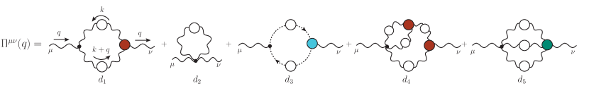
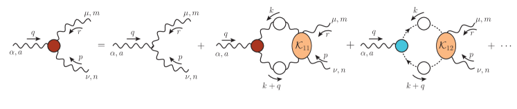
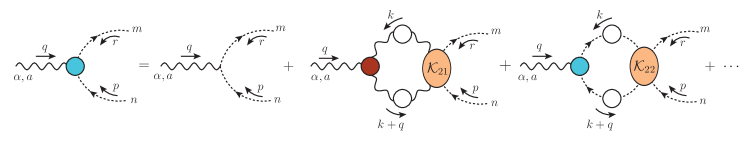
Figure 1: First row: The diagrammatic representation of the gluon self-energy. Second row: The SDE for the three-gluon vertex. Third row: The SDE for the ghost-gluon vertex. White (colored) circles denote fully dressed propagators (vertices), while the orange ellipses denote four-particle kernels.

We next turn to the three-point sector of the theory, which, in the absence of dynamical quarks, contains the three-gluon and the ghost-gluon vertices, denoted by

$${\rm{I}}\!\Gamma^{abc}_{\alpha\mu\nu}(q,r,p)=gf^{abc}\,{\rm{I}}\!\Gamma_{\alpha\mu\nu}(q,r,p)\,,\qquad\qquad{\rm{I}}\!\Gamma_{\mu}^{mna}(r,p,q)=-gf^{mna}\,{\rm{I}}\!\Gamma_{\mu}(r,p,q)\,,$$ (8)

where all momenta are incoming, $q+p+r=0$. The corresponding SDEs that govern the evolution of ${\rm{I}}\!\Gamma_{\alpha\mu\nu}(q,r,p)$ and ${\rm{I}}\!\Gamma_{\mu}(r,p,q)$ are shown in the second and third row of Fig. 1, respectively Schleifenbaum et al. (2005); Huber and von Smekal (2013); Aguilar et al. (2013b); Huber et al. (2012); Blum et al. (2014); Eichmann et al. (2014); Williams et al. (2016); Aguilar et al. (2018); Huber (2020); Papavassiliou et al. (2022). The omitted terms, indicated by ellipses, contain the fully-dressed four-gluon vertex (with incoming momentum $q$). In general, these latter contributions are technically harder to compute; nonetheless, related studies seem to suggest that their impact on our analysis is likely to be rather small Williams et al. (2016); Huber (2020).

Note that in Fig. 1 we show the Bethe-Salpeter version of the vertex SDE, whose main difference is that, inside the loops, the tree-level vertices (with incoming momentum $q$) have been replaced by their fully-dressed counterparts. This substitution may be carried out provided that the corresponding four-particle kernels ${\cal K}_{ij}$ have been modified accordingly, in order to avoid overcounting. For example, ladder graphs (straight boxes) must be omitted, while cross-ladder (crossed boxes) are retained (see e.g., Fig. 7 of Aguilar et al. (2012)). This particular formulation of the SDE offers an important technical advantage: vertex renormalization constants, which otherwise would appear explicitly multiplying individual diagrams, are fully absorbed by the additional dressed vertices (see Sec. V).

The algebraic manipulations of potentially divergent integrals require the use of symmetry-preserving regularization schemes. This is particularly important, because a flawed regularization procedure may introduce artifacts that mimic the effects of a gluon mass. Dimensional regularization Collins (1986) is especially well-suited for this purpose, and will be adopted in what follows. Note, in fact, that its use is crucial for the demonstration of the seagull identity Aguilar and Papavassiliou (2010); Aguilar et al. (2016b) (see Sec. IX), whose validity, in turn, guarantees the nonperturbative masslessness of the gluon, when the Schwinger mechanism is not activated.

For the loop integrals regularized with dimensional regularization we introduce the short-hand notation

$$\int_{k}:=\frac{\mu_{{\scriptscriptstyle 0}}^{\epsilon}}{(2\pi)^{d}}\!\int_{-\infty}^{+\infty}\!\!\mathrm{d}^{d}k\,,$$ (9)

where $d=4-\epsilon$ is the dimension of the space-time, and $\mu_{{\scriptscriptstyle 0}}$ denotes the ’t Hooft mass. It is understood that the regularization is employed until certain crucial cancellations have taken place, and the procedure of renormalization has been duly carried out. Past that point, the resulting equations are finite, and no regularization is needed.

III Schwinger mechanism in Yang-Mills theories

Endowing gauge bosons with a mass in a field-theoretically consistent way is particularly subtle. In this section we review the generation of a gluon mass through the nonperturbative realization of the well-known Schwinger mechanism Schwinger (1962a, b) in the context of a Yang-Mills theory described by Eq. (1).

The general idea of the mechanism is best expressed in terms of the dimensionless vacuum polarization, $\overline{\Pi}(q^{2})$, defined in terms of the gluon self-energy ${\Pi}(q^{2})$ through ${\Pi}(q^{2})=q^{2}\overline{\Pi}(q^{2})$, such that

$$\Delta^{-1}({q^{2}})=q^{2}[1+i\overline{\Pi}(q^{2})]\,.$$ (10)

Schwinger’s fundamental observation states that if the vacuum polarization $\overline{\Pi}(q^{2})$ develops a pole at zero momentum transfer ($q^{2}=0$), then the vector meson (gluon) acquires a mass, even if the gauge symmetry prohibits the inclusion of a mass term at the level of the defining Lagrangian. Thus, one has

$$\lim_{q\to 0}i\overline{\Pi}(q^{2})=m^{2}/q^{2}\,\,\Longrightarrow\,\,\lim_{q\to 0}\,\Delta^{-1}(q^{2})=\lim_{q\to 0}\,(q^{2}+m^{2})\,\,\Longrightarrow\,\,\Delta^{-1}(0)=m^{2}\,,$$ (11)

and the vector meson picks up a mass, in the sense that its propagator at the origin saturates at a finite nonvanishing value, which is determined by the (positive) residue of the pole.

The argument described above is completely general, and its key conclusion does not depend on the dynamical details that lead to the appearance of a massless pole in $\overline{\Pi}(q^{2})$. Of course, in practice, depending on the characteristics of each theory, the circumstances that trigger the sequence described in Eq. (11) may be very distinct Jackiw and Johnson (1973); Jackiw (1973). In the case of Yang-Mills theories, the origin of the pole is purely dynamical, as first described in the classic work by Eichten and Feinberg Eichten and Feinberg (1974). In what follows we will present the modern implementation of this scenario, as it has been developed in a series of articles during the past few years.

The general idea is that the nonperturbative vertices of the theory develop special massless composite excitations, which find their way into the gluon vacuum polarization through the SDE of Fig. 1 Aguilar et al. (2012); Binosi et al. (2012); Ibañez and Papavassiliou (2013); Binosi and Papavassiliou (2018); Aguilar et al. (2018). In particular, the three-gluon and ghost-gluon vertices assume the general form (see Fig. 2)

$${\rm{I}}\!\Gamma_{\alpha\mu\nu}(q,r,p) = \Gamma_{\alpha\mu\nu}(q,r,p)+V_{\alpha\mu\nu}(q,r,p)\,,\qquad$$

$${\rm{I}}\!\Gamma_{\alpha}(q,r,p) = \Gamma_{\alpha}(q,r,p)+V_{\alpha}(q,r,p)\,,$$ (12)

where $\Gamma_{\alpha\mu\nu}(q,r,p)$ and $\Gamma_{\alpha}(r,p,q)$ are the pole-free components of the two vertices, while $V_{\alpha\mu\nu}(q,r,p)$ and $V_{\alpha}(q,r,p)$ contain longitudinally coupled bound-state poles, i.e., of the special tensorial structure

$$V_{\alpha\mu\nu}(q,r,p) = \frac{q_{\alpha}}{q^{2}}C_{\mu\nu}(q,r,p)+\frac{r_{\mu}}{r^{2}}A_{\alpha\nu}(q,r,p)+\frac{p_{\nu}}{p^{2}}B_{\alpha\mu}(q,r,p)\,,$$

$$V_{\alpha}(q,r,p) = \frac{q_{\alpha}}{q^{2}}C(q,r,p)\,.$$ (13)

We emphasize that the pole-free components are not “regular” functions, in the strict sense of the term, because certain of their form factors diverge logarithmically in the infrared, see,e.g., Aguilar et al. (2014a). Note also that the corresponding tree-level expressions are given by

$$\Gamma_{\!0}^{\alpha\mu\nu}(q,r,p)=(q-r)^{\nu}g^{\alpha\mu}+(r-p)^{\alpha}g^{\mu\nu}+(p-q)^{\mu}g^{\nu\alpha}\,,\qquad\qquad\Gamma_{\!0}^{\alpha}(q,r,p)=r^{\alpha}\,.$$ (14)

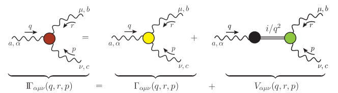
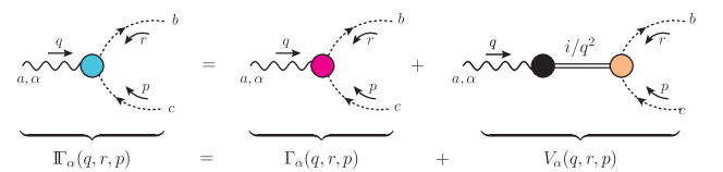
Figure 2: The diagrammatic representation of the three-gluon and ghost-gluon vertices introduced in Eq. (12): ${\rm{I}}\!\Gamma_{\alpha\mu\nu}(q,r,p)$ (first row) and ${\rm{I}}\!\Gamma_{\alpha}(q,r,p)$ (second row). The first term on the r.h.s. indicates the pole-free part, $\Gamma_{\alpha\mu\nu}(q,r,p)$ or $\Gamma_{\alpha}(q,r,p)$, while the second denotes the pole term $V_{\alpha\mu\nu}(q,r,p)$ or $V_{\alpha}(q,r,p)$.

The longitudinal nature of the $V_{\alpha\mu\nu}(q,r,p)$ and $V_{\alpha}(q,r,p)$ is easily established at the level of Fig. 2. Specifically, the black circle denotes the transition amplitude, $I_{\alpha}(q)$, connecting a gluon with a (massless composite) scalar; since this amplitude depends on a single momentum, $q$, and a single Lorentz index, $\alpha$, its general form is simply $I_{\alpha}(q)=q_{\alpha}I(q^{2})$, where $I(q^{2})$ is a scalar form factor Aguilar et al. (2012); Ibañez and Papavassiliou (2013). In the case of $V_{\alpha\mu\nu}(q,r,p)$, Bose symmetry enforces the same property in the remaining two channels, thus finally accounting for the general form given in Eq. (13). The form factor $I(q^{2})$ is eventually absorbed into $C(q,r,p)$ and $C_{\mu\nu}(q,r,p)$; additional details on the structure of $I_{\alpha}(q)$ will be given in Sec. X.

An immediate consequence of Eq. (13) is that $V_{\alpha\mu\nu}(q,r,p)$ and $V_{\alpha}(q,r,p)$ satisfy the crucial relations

$${P}_{\alpha^{\prime}}^{\alpha}(q){P}_{\mu^{\prime}}^{\mu}(r){P}_{\nu^{\prime}}^{\nu}(p)V_{\alpha\mu\nu}(q,r,p)=0\,,\qquad{P}_{\alpha^{\prime}}^{\alpha}(q)V_{\alpha}(q,r,p)=0\,;$$ (15)

therefore, they drop out from the typical quantities studied on the lattice, which involve the transversely projected vertices [see, e.g., Eq. (75)]. In fact, as we will see in detail in Sec. XI, Eq. (15) is instrumental for the cancellation of all pole divergences from physical observables, such as $S$-matrix elements.

Note that, even though $V_{\alpha\mu\nu}(q,r,p)$ possesses poles in all three of its channels, only the one associated with the $q$-channel, i.e., the channel that carries the physical momentum entering in the gluon propagator, is actually relevant. In fact, the longitudinal structure of $V_{\alpha\mu\nu}(q,r,p)$, together with the fact that we work in the Landau gauge, and hence, gluon propagators inside Feynman diagrams are transverse, leads to the simplification

$${P}_{\mu^{\prime}}^{\mu}(r){P}_{\nu^{\prime}}^{\nu}(p)V_{\alpha\mu\nu}(q,r,p)=\frac{q_{\alpha}}{q^{2}}{P}_{\mu^{\prime}}^{\mu}(r){P}_{\nu^{\prime}}^{\nu}(p)C_{\mu\nu}(q,r,p)\,.$$ (16)

Thus, for our analysis we only require the tensorial decomposition of the term $C_{\mu\nu}(q,r,p)$ in Eq. (13), given by

$$C_{\mu\nu}(q,r,p)=C_{1}\,g_{\mu\nu}+C_{2}\,r_{\mu}r_{\nu}+C_{3}\,p_{\mu}p_{\nu}+C_{4}\,r_{\mu}p_{\nu}+C_{5}\,p_{\mu}r_{\nu}\,,$$ (17)

where $C_{j}:=C_{j}(q,r,p)$. Now, when the $C_{\mu\nu}(q,r,p)$ of Eq. (17) is substituted into Eq. (16), and the relation $q+p+r=0$ is appropriately employed, only two form factors survive,

$${P}_{\mu^{\prime}}^{\mu}(r){P}_{\nu^{\prime}}^{\nu}(p)V_{\alpha\mu\nu}(q,r,p)=\frac{q_{\alpha}}{q^{2}}{P}_{\mu^{\prime}}^{\mu}(r){P}_{\nu^{\prime}}^{\nu}(p)\left[C_{1}\,g_{\mu\nu}+C_{5}q_{\mu}q_{\nu}\right]\,.$$ (18)

Since we are mostly interested in the behavior of the gluon propagator at the origin, in what follows we will be expanding the relevant equations around $q=0$, keeping terms at most linear in $q$. In such an expansion, the term proportional to $C_{5}$ in Eq. (18) is subleading, being of order ${\cal O}(q^{2})$. So, finally, one ends up with a single relevant form factor per pole vertex, namely $C_{1}(q,r,p)$, related to $V_{\alpha\mu\nu}(q,r,p)$, and $C(q,r,p)$, the unique component of $V_{\alpha}(q,r,p)$.

In what follows we will repeatedly use the Taylor expansion of a function $f(q,r,p)$ around $q=0$ ($p=-r$), given by

$$\lim_{q\to 0}f(q,r,p) = f(0,r,-r)+q^{\alpha}\left[\frac{\partial f(q,r,p)}{\partial q^{\alpha}}\right]_{q=0}+\cdots\,,$$ (19)

$$= f(0,r,-r)+2(q\cdot r)\left[\frac{\partial f(q,r,p)}{\partial p^{2}}\right]_{q=0}+\cdots\,.$$

where the ellipses denote terms of ${\cal O}(q^{2})$ or higher.

There are two important results relevant for the Taylor expansion of $C_{1}(q,r,p)$ and $C(q,r,p)$, namely

$$C_{1}(0,r,-r)=0\,,\qquad\qquad C(0,r,-r)=0\,.$$ (20)

The first relation follows directly from the Bose symmetry of the three-gluon vertex, which implies that $C_{1}(q,r,p)=-C_{1}(q,p,r)$. The justification of the second relation in Eq. (20) is less immediate, relying on special relations Binosi and Papavassiliou (2002a, 2009) linking ${\rm{I}}\!\Gamma_{\alpha}(q,r,p)$ with the vertex $\widetilde{\Gamma}_{\alpha}(q,r,p)$ introduced in Sec. VI. As we will see in Sec. VII, the first relation in Eq. (20) will be derived in a completely independent way from the fundamental WIs satisfied by the three-gluon vertex.

In view of Eq. (20), the Taylor expansion of ${C}_{1}(q,r,p)$ and ${C}(q,r,p)$ around $q=0$ yields

$$\lim_{q\to 0}{C}_{1}(q,r,p)=2(q\cdot r){\mathbb{C}}(r^{2})\,+\cdots\,,\qquad\lim_{q\to 0}{C}(q,r,p)=2(q\cdot r){\cal C}(r^{2})\,+\cdots\,,$$ (21)

with

$${\mathbb{C}}(r^{2}):=\left[\frac{\partial{C}_{1}(q,r,p)}{\partial p^{2}}\right]_{q=0}\,,\qquad\qquad{\cal C}(r^{2}):=\left[\frac{\partial{C}(q,r,p)}{\partial p^{2}}\right]_{q=0}\,.$$ (22)

The functions ${\mathbb{C}}(r^{2})$ and ${\cal C}(r^{2})$ are central to the ensuing analysis. In particular, there are three pivotal points related to them that will be elucidated in the next sections. First, we will prove that nonvanishing ${\mathbb{C}}(r^{2})$ and ${\cal C}(r^{2})$ do indeed emerge from the corresponding dynamical equations for ${\rm{I}}\!\Gamma_{\alpha\mu\nu}(q,r,p)$ and ${\rm{I}}\!\Gamma_{\alpha}(q,r,p)$. In fact, as we will see in the next section, these two functions turn out to be the BS amplitudes describing the formation of a gluon-gluon and a ghost-antighost colored composite bound state, respectively. Second, we will derive the formula that expresses the gluon mass in terms of ${\mathbb{C}}(r^{2})$ and ${\cal C}(r^{2})$, and will demonstrate that it furnishes a result compatible with the lattice simulations; that will be the subject of Sec. V. Third, in Sec. VI we will elaborate on the notion of the WI displacement, and show that ${\mathbb{C}}(r^{2})$ corresponds precisely to the displacement function that quantifies the modification of the WIs satisfied by $\Gamma_{\alpha\mu\nu}(q,r,p)$ in the presence of massless poles.

IV Dynamical formation of massless poles

We next turn to the study of the precise dynamics that leads to the formation of the poles that comprise the components $V_{\alpha\mu\nu}(q,r,p)$ and $V_{\alpha}(q,r,p)$ entering in Eq. (13). The fundamental equations that control this process are the SDEs for ${\rm{I}}\!\Gamma_{\alpha\mu\nu}(q,r,p)$ and ${\rm{I}}\!\Gamma_{\alpha}(q,r,p)$, which, in the limit $q\to 0$, provide a set of linear BSEs for the quantities ${\mathbb{C}}(r^{2})$ and ${\cal C}(r^{2})$, defined in Eqs. (21) and (22).

In what follows we set $\lambda:=ig^{2}C_{\rm A}/2$, where $C_{\mathrm{A}}$ is the Casimir eigenvalue of the adjoint representation [$N$ for $SU(N)$]. Then, the system of SDEs shown in Fig. 1 assumes the form Aguilar et al. (2022)

$${\rm{I}}\!\Gamma^{\alpha\mu\nu} = \Gamma_{\!0}^{\alpha\mu\nu}-\lambda\int_{k}{\rm{I}}\!\Gamma^{\alpha\beta\gamma}\Delta_{\beta\rho}\Delta_{\gamma\sigma}{\cal K}_{11}^{\mu\nu\sigma\rho}+2\lambda\int_{k}{\rm{I}}\!\Gamma^{\alpha}DD{\cal K}_{12}^{\mu\nu}\,,$$

$${\rm{I}}\!\Gamma^{\alpha} = \Gamma_{\!0}^{\alpha}-\lambda\int_{k}{\rm{I}}\!\Gamma^{\alpha\beta\gamma}\Delta_{\beta\rho}\Delta_{\gamma\sigma}{\cal K}_{21}^{\sigma\rho}-\lambda\int_{k}{\rm{I}}\!\Gamma^{\alpha}DD{\cal K}_{22}\,,$$ (23)

where, for compactness, all momentum arguments, indicated explicitly on the diagrams of Fig. 1, have been suppressed.

Next, we substitute into Eq. (23) the expressions for the fully-dressed vertices given in Eq. (12). In addition, in order to exploit Eq. (18), the first of the two equations is multiplied by the factor ${P}_{\mu^{\prime}\mu}(r){P}^{\mu^{\prime}}_{\nu}(p)$. Then, as the limit $q\to 0$ is taken, two tensorial structures emerge: one associated with the pole-free terms, which is proportional to $r^{\alpha}$, and one associated with the pole terms, being proportional to $q^{\alpha}$. The matching of the terms proportional to $q^{\alpha}$ on both sides leads to the desired BSEs, while the matching of the terms proportional to $r^{\alpha}$ furnishes a dynamical system for the so-called “soft-gluon” form-factors of $\Gamma_{\alpha\mu\nu}(q,r,p)$ and $\Gamma_{\alpha}(q,r,p)$ [see, for example, Eq. (68)]. Focusing on the BSEs, the limit $q\to 0$ activates Eq. (21), and the functions ${\mathbb{C}}(r^{2})$ and ${\mathbb{C}}(r^{2})$ make their appearance.

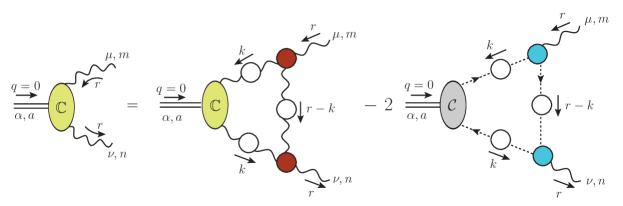
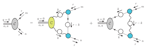
Figure 3: The diagrammatic representation of the coupled system of BSEs that governs the evolution of the functions ${\mathbb{C}}(r^{2})$ and ${\cal C}(r^{2})$.

Specifically, after employing the useful relation

$$\int_{k}(q\cdot k)\,f(k,r)=\frac{(q\cdot r)}{r^{2}}\int_{k}(r\cdot k)\,f(k,r)\,,$$ (24)

with $f(k,r)$ denoting a generic kernel, we arrive at a system of homogeneous equations involving ${\mathbb{C}}(r^{2})$ and ${\mathcal{C}}(r^{2})$, namely (see Fig. 3)

$${\mathbb{C}}(r^{2}) = -\frac{\lambda}{3}\int_{k}{\mathbb{C}}(k^{2})\Delta^{2}(k^{2})P_{\rho\sigma}(k)P_{\mu\nu}(r)\widetilde{\cal K}_{11}^{\mu\nu\sigma\rho}+\frac{2\lambda}{3}\int_{k}{\mathcal{C}}(k^{2})D^{2}(k^{2})P_{\mu\nu}(r)\widetilde{\cal K}_{12}^{\mu\nu}\,,$$

$${\mathcal{C}}(r^{2}) = -\lambda\int_{k}{\mathbb{C}}(k^{2})\Delta^{2}(k^{2})P_{\sigma\rho}(k)\widetilde{\cal K}_{21}^{\sigma\rho}-\lambda\int_{k}{\mathcal{C}}(k^{2})D^{2}(k^{2})\widetilde{\cal K}_{22}\,,$$ (25)

where $\widetilde{\cal K}_{ij}:=(r\cdot k/r^{2})\,{\cal K}_{ij}(r,-r,k,-k)$. Note that the above derivation has been carried out in Minkowski space, and hence the imaginary factor of $i$ in the definition of $\lambda$. Before proceeding with the numerical analysis, the result must be passed to the Euclidean space, following standard conversion rules. Note, in particular, that the integral measure changes according to $d^{4}k\to id^{4}k_{{\scriptscriptstyle\rm E}}$; this additional factor of $i$ combines with $\lambda$ to yield real expressions.

The system of integral equations given in Eq. (25) are the BSEs that govern the formation of massless colored bound states out of two gluons and a ghost-antighost pair; the functions ${\mathbb{C}}(r^{2})$ and ${\mathcal{C}}(r^{2})$ are the corresponding BS amplitudes. It is therefore of the utmost importance to find nontrivial solutions for these functions, even if certain simplifying assumptions will be implemented at the level of the ingredients entering in Eq. (25).

To that end, we employ the “one-particle exchange” approximation for the kernels ${\cal K}_{ij}$, shown in Fig. 4; the ingredients required for their evaluation are the fully dressed propagators and vertices. Note that only the pole-free parts $\Gamma_{\alpha\mu\nu}$ and $\Gamma_{\alpha}$ are relevant for the evaluation of the kernels ${\cal K}_{ij}$, because the various projections implemented during the derivation of Eq. (25) activate Eq. (15); the reader is referred to Aguilar et al. (2022), and in particular Appendix A therein, for further details.

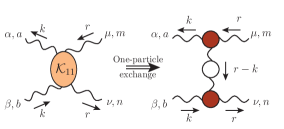
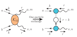
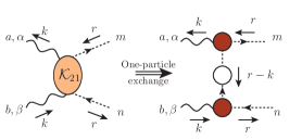
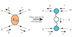
Figure 4: The one-particle exchange approximations of the kernels ${\cal K}_{ij}$, and the associated kinematic conventions.

The system of integral equations in Eq. (25) is linear and homogeneous in the unknown functions, thus corresponding to an eigenvalue problem, which finally singles out a special value for the strong coupling, $\alpha_{s}=g^{2}/4\pi$. Specifically, we find that $\alpha_{s}=0.63$ when the renormalization point $\mu=4.3$ GeV. For this particular value of $\alpha_{s}$, we find nontrivial solutions for ${\mathbb{C}}(r^{2})$ and ${\mathcal{C}}(r^{2})$, which are shown in the left panel of Fig. 5. This value of $\alpha_{s}$ is to be contrasted with the corresponding value obtained within the concrete renormalization scheme that we employ. Specifically, we work within the general framework of the momentum subtraction (MOM) scheme Hasenfratz and Hasenfratz (1980), where two-point functions acquire their tree-level expressions at a given scale $\mu$, i.e., $\Delta^{-1}_{{\scriptscriptstyle R}}(\mu^{2})=\mu^{2}$. Within this scheme we adapt the so-called asymmetric version Alles et al. (1997); Davydychev et al. (1998); Boucaud et al. (1998a, b); Athenodorou et al. (2016); Aguilar et al. (2020a), characterized by the condition $\mathit{L}_{{sg}}(\mu^{2})=1$, where $\mathit{L}_{{sg}}(r^{2})$ is the form factor of the three-gluon vertex in the soft-gluon (“asymmetric”) configuration, see Eq. (75); the estimated value of $\alpha_{s}$ within this scheme is $\alpha_{s}=0.27$ Athenodorou et al. (2016); Aguilar et al. (2020a).

It is of course natural to interpret this numerical discrepancy in the values of $\alpha_{s}$ as an artifact of the truncation employed, and especially the approximation of the kernels ${\cal K}_{ij}$ by their one-particle exchange diagrams. It is worth mentioning that, according to a preliminary analysis, moderate modifications of the kernel affect the value of $\alpha_{s}$ considerably, leaving the form of the solutions found for ${\mathbb{C}}_{\star}(r^{2})$ and ${\mathcal{C}}_{\star}(r^{2})$ essentially unmodified. This observation implies that a more complete knowledge of the corresponding BSE kernels is required in order to decrease $\alpha_{s}$ towards its correct MOM value. On the other hand, the solutions obtained with the approximations described above should be considered as fairly reliable.

It is important to stress that, due to the homogeneity and linearity of Eq. (25), the overall scale of the solutions is undetermined, since the multiplication of a given solution by an arbitrary real constant produces another solution. In the case of the solutions shown in Fig. 5, denoted by ${\mathbb{C}}_{\star}(r^{2})$ and ${\mathcal{C}}_{\star}(r^{2})$, the scale has been fixed by requiring the best possible matching with the corresponding result obtained for ${\mathbb{C}}(r^{2})$ from the WI displacement in Sec. VIII. This scale ambiguity originates from considering only the leading order terms of the BSEs in the expansion around $q=0$; it may be resolved if further orders in $q$ are kept, because of the additional inhomogeneous terms that they induce, see, e.g., Nakanishi (1969); Maris and Roberts (1997); Blank and Krassnigg (2011).

Note finally that ${\mathbb{C}}_{\star}(r^{2})$ is considerably larger in magnitude than ${\mathcal{C}}_{\star}(r^{2})$ Aguilar et al. (2018), indicating that the three-gluon vertex accounts for the bulk of the gluon mass.

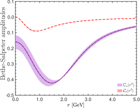
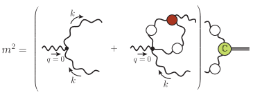
Figure 5: Left panel: The solutions for ${\mathbb{C}}_{\star}(r^{2})$ (purple dot-dashed) and ${\mathcal{C}}_{\star}(r^{2})$ (red dashed) obtained from the coupled BSE system of Eq. (25). Right panel: Diagrammatic representation of the mass term that emerges from the insertion of the pole term $V_{\nu\alpha^{\prime}\beta^{\prime}}$ into the diagrams $d_{1}$ and $d_{4}$ of Fig. 1.

V Gluon mass via the Schwinger mechanism

In this section we elucidate in some detail on how the inclusion of vertices with massless poles into the gluon SDE triggers the Schwinger mechanism, leading to the generation of a gluon mass.

In order to fix the ideas, let us consider a specific example, namely the diagram $d_{1}^{\mu\nu}(q)$ shown in the first row of Fig. 1, corresponding to the expression

$$id_{1}^{\mu\nu}(q)=\lambda\int_{k}{\Gamma}^{\mu\alpha\beta}_{0}(q,k,-k-q)\Delta_{\alpha\alpha^{\prime}}(k)\Delta_{\beta\beta^{\prime}}(k+q){\rm{I}}\!\Gamma^{\nu\alpha^{\prime}\beta^{\prime}}(q,k,-k-q)\,.$$ (26)

Let us next use for ${\rm{I}}\!\Gamma^{\nu\alpha^{\prime}\beta^{\prime}}(q,k,-k-q)$ a three-gluon vertex containing the type of massless poles described above (evidently with the appropriate relabelling of indices). In particular, substitute into Eq. (26) the vertex given in the first equation of Eq. (12), with $\{\alpha,\mu,\nu\}\to\{\nu,\alpha^{\prime},\beta^{\prime}\}$, and denote by ${\widehat{d}}_{1}^{\,\mu\nu}(q)$ the contribution originating exclusively from the term $V_{\nu\alpha^{\prime}\beta^{\prime}}(q,k,-k-q)$, namely

$$i{\widehat{d}}_{1}^{\,\mu\nu}(q)=\lambda\int_{k}{\Gamma}^{\mu\alpha\beta}_{0}(q,k,-k-q)\Delta_{\alpha\alpha^{\prime}}(k)\Delta_{\beta\beta^{\prime}}(k+q)V^{\nu\alpha^{\prime}\beta^{\prime}}(q,k,-k-q)\,.$$ (27)

Now, from the general form of $V^{\alpha\mu\nu}$ given in Eq. (13) it is evident that, since we work in the Landau gauge, the only term that survives in Eq. (27) is proportional to $C^{\alpha^{\prime}\beta^{\prime}}(q,k,-k-q)$, such that

$$i{\widehat{d}}_{1}^{\,\mu\nu}(q)=\lambda\frac{q^{\nu}}{q^{2}}\int_{k}{\Gamma}^{\mu\alpha\beta}_{0}(q,k,-k-q)\Delta_{\alpha\alpha^{\prime}}(k)\Delta_{\beta\beta^{\prime}}(k+q)C^{\alpha^{\prime}\beta^{\prime}}(q,k,-k-q)\,.$$ (28)

Clearly, ${\widehat{d}}_{1}^{\,\mu\nu}(q)$ can only be proportional to $q^{\mu}q^{\nu}$; so, we set ${\widehat{d}}_{1}^{\,\mu\nu}(q)=(q^{\mu}q^{\nu}/q^{2}){\widehat{d}}_{1}(q^{2})$, with

$$i{\widehat{d}}_{1}(q^{2})=\lambda\frac{q_{\mu}}{q^{2}}\int_{k}{\Gamma}^{\mu\alpha\beta}_{0}(q,k,-k-q)\Delta_{\alpha\alpha^{\prime}}(k)\Delta_{\beta\beta^{\prime}}(k+q)C_{\alpha^{\prime}\beta^{\prime}}(q,k,-k-q)\,.$$ (29)

We next determine ${\widehat{d}}_{1}(0)$,

$$i{\widehat{d}}_{1}(0)=\lambda\frac{q_{\mu}}{q^{2}}\,\lim_{q\to 0}\,\int_{k}{\Gamma}_{0}^{\mu\alpha\beta}(q,k,-k-q)\Delta_{\alpha\alpha^{\prime}}(k)\Delta_{\beta\beta^{\prime}}(k+q)C^{\alpha^{\prime}\beta^{\prime}}(q,k,-k-q)\,.$$ (30)

The expansion of the integrand around $q=0$ proceeds by inserting Eq. (21) and setting $q=0$ elsewhere, yielding

$$i{\widehat{d}}_{1}(0)=2\lambda\,\frac{q_{\mu}q_{\nu}}{q^{2}}\int_{k}k^{\nu}{\Gamma}_{0}^{\mu\alpha\beta}(0,k,-k)P_{\alpha\beta}(k)\Delta^{2}(k^{2}){\mathbb{C}}(k^{2})\,,$$ (31)

with

$${\Gamma}_{0}^{\mu\alpha\beta}(0,k,-k)=2k^{\mu}g^{\alpha\beta}-k^{\alpha}g^{\mu\beta}-k^{\beta}g^{\mu\alpha}\,.$$ (32)

Since the integral is proportional to $g^{\mu\nu}$, we find (using that $g_{\mu}^{\mu}=4$ and $P_{\mu}^{\mu}(q)=3$)

$$i{\widehat{d}}_{1}(0) = \frac{\lambda}{2}\int_{k}k_{\mu}{\Gamma}_{0}^{\mu\alpha\beta}(0,k,-k)P_{\alpha\beta}(k)\Delta^{2}(k^{2}){\mathbb{C}}(k^{2})$$ (33)

$$= 3\lambda\int_{k}k^{2}\Delta^{2}(k^{2}){\mathbb{C}}(k^{2})\,.$$

To establish explicit contact with the formulation by Schwinger described in Sec. III, notice that the contribution of ${\widehat{d}}_{1}^{\,\mu\nu}(q)$ to the gluon vacuum polarization, $\overline{\Pi}(q^{2})$, is simply given by ${\widehat{d}}_{1}(0)/q^{2}$; as advocated, it amounts to a massless pole, whose residue is precisely ${\widehat{d}}_{1}(0)$.

The full computation of the total gluon mass proceeds by including the effects of diagrams $d_{3}$ and $d_{4}$, shown in the first line of Fig. 1. Specifically, diagram $d_{4}$ will contribute to the mass for the same reason as $d_{1}$, namely due to the insertion of the massless pole associated with the three-gluon vertex, proportional to $C_{\alpha^{\prime}\beta^{\prime}}$; eventually, after the limit $q\to 0$ has been taken, ${\mathbb{C}}(k^{2})$ emerges once again. As a result, the corresponding contributions from $d_{1}$ and $d_{4}$ may be naturally combined into a single expression, whose diagrammatic representation is given in the right panel of Fig. 5. Note that the contribution from graph $d_{4}$ contains a function denoted by $Y(k^{2})$, given by Binosi et al. (2012)

$$Y(k^{2})=\frac{i\lambda}{2k^{2}}\,k^{\rho}\int_{\ell}\Delta_{\mu\rho}(\ell)\Delta_{\alpha\nu}(\ell+k)\Gamma^{\alpha\mu\nu}(k,\ell,-k-\ell)\,,$$ (34)

whose origin is the one-loop subdiagram nested inside $d_{4}$. In addition, the contribution of $d_{3}$ originates from the pole in the fully-dressed ghost-gluon vertex, ${\rm{I}}\!\Gamma_{\alpha}$, in accordance with Eqs. (12) and (13); it is proportional to $C(q,r,p)$, and once the limit $q\to 0$ has been implemented, to ${\cal C}(k^{2})$.

As with any SDE computation, multiplicative renormalization must be implemented following the standard rules. In particular, we introduce the renormalized fields and coupling constant Aguilar et al. (2014b)

$$A^{a\,\mu}_{{\scriptscriptstyle R}}(x)=Z^{-1/2}_{{\scriptscriptstyle A}}A^{a\,\mu}(x)\,,\qquad c_{{\scriptscriptstyle R}}^{a}(x)=Z^{-1/2}_{c}c^{a}(x)\,,\qquad g_{{\scriptscriptstyle R}}=Z_{g}^{-1}g\,,$$ (35)

such that the associated two point functions are renormalized as

$$\Delta_{{\scriptscriptstyle R}}(q^{2})=Z^{-1}_{{\scriptscriptstyle A}}\Delta(q^{2})\,,\qquad D_{{\scriptscriptstyle R}}(q^{2})=Z^{-1}_{c}D(q^{2})\,.$$ (36)

Similarly, the renormalization constants of the three fundamental Yang-Mills vertices (ghost-gluon, three-gluon, and four-gluon) are defined as

$${\rm{I}}\!\Gamma^{\mu}_{\!\!{\scriptscriptstyle R}}=\widetilde{Z}_{1}{\rm{I}}\!\Gamma^{\mu};\qquad{\rm{I}}\!\Gamma^{\mu\alpha\beta}_{\!\!{\scriptscriptstyle R}}=Z_{3}{\rm{I}}\!\Gamma^{\mu\alpha\beta};\qquad{\rm{I}}\!\Gamma^{\mu\alpha\beta\nu}_{\!\!{\scriptscriptstyle R}}=Z_{4}{\rm{I}}\!\Gamma^{\mu\alpha\beta\nu}.$$ (37)

In addition, we employ the following set of exact relations

$$Z_{g}=\widetilde{Z}_{1}Z_{{\scriptscriptstyle A}}^{-1/2}Z_{c}^{-1}=Z_{3}Z_{{\scriptscriptstyle A}}^{-3/2}=Z_{4}^{1/2}Z_{{\scriptscriptstyle A}}^{-1}\,,$$ (38)

which are enforced by the STIs of the theory. Once the renormalization procedure has been completed, the subscript “$\rm R$” will be suppressed from all quantities, in order to avoid notational clutter.

Next we pass the answer to Euclidean space and make standard use of the hyperspherical coordinates, carrying out the trivial angular integrations. The final result reads

$$m^{2}=3\hat{\lambda}\int_{0}^{\infty}\!\!dy\,\mathcal{Z}^{2}(y)\left[6\pi\alpha_{s}C_{\mathrm{A}}Z_{4}Y(y)-Z_{3}\right]{\mathbb{C}}(y)\,+\,\hat{\lambda}\,\widetilde{Z}_{1}\int_{0}^{\infty}\!\!dy\,F^{2}(y)\,{\cal C}(y)\,,$$ (39)

where we have employed the gluon and ghost dressing functions, $\mathcal{Z}(q^{2})$ and $F(q^{2})$, introduced in Eqs. (2) and (7), respectively, and have set $\hat{\lambda}:=C_{\mathrm{A}}\alpha_{s}/8\pi$.

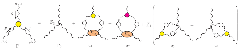
Figure 6: The SDE satisfied by the pole-free part of the renormalized three-gluon vertex, with the vertex renormalization constants $Z_{3}$ and $Z_{4}$ explicitly indicated. The symmetry factor of diagrams $a_{3}$ and $a_{4}$ is $\frac{1}{2}$.

Turning to the renormalization constants appearing in Eq. (39), let us first point out that, in the Landau gauge, $\widetilde{Z}_{1}$ has a finite, cutoff-independent value, by virtue of Taylor’s theorem Taylor (1971); in fact, in the so-called “Taylor scheme” Boucaud et al. (2009); von Smekal et al. (2009); Boucaud et al. (2011), we have that $\widetilde{Z}_{1}=1$. However, in our analysis we will employ the “asymmetric” MOM scheme mentioned earlier, which yields a slightly lower value, $\widetilde{Z}_{1}\approx 0.95$ Aguilar et al. (2021a). On the other hand, both $Z_{3}$ and $Z_{4}$ are cutoff-dependent, thus complicating considerably the use of Eq. (39).

To circumvent this difficulty, consider the renormalized SDE of the pole-free part, $\Gamma^{\alpha\mu\nu}$, shown in Fig. 6; the renormalization constants that survive, after the relations in Eq. (38) have been duly employed, are explicitly shown. It is relatively straightforward to establish that the sum

$${\cal G}^{\mu\alpha\beta}(q,r,p):=Z_{3}{\Gamma}^{\mu\alpha\beta}_{0}(q,r,p)+Z_{4}\left[{a}^{\mu\alpha\beta}_{3}(q,r,p)+{a}^{\mu\alpha\beta}_{4}(q,r,p)\right]$$ (40)

is precisely the combination of vertex diagrams that appears inside the kernel of the mass equation (right panel of Fig. 5), in the special momentum configuration ${\cal G}^{\mu\alpha\beta}(0,k,-k)$ Aguilar et al. (2014b). Note that the graphs $a_{3}$ and $a_{4}$, after appropriate symmetrization, generate precisely the contribution associated with the function $Y(k^{2})$; in fact, the symmetry factor of the diagrams $a_{3}$ and $a_{4}$ is $\frac{1}{2}$, exactly as needed for reaching Eq. (40).

Then, if we set

$${\cal G}^{\mu\alpha\beta}(0,k,-k)=2{\cal G}(k^{2})\,k^{\mu}g^{\alpha\beta}+\cdots\,,$$ (41)

where the ellipsis indicates contributions proportional to $k^{\alpha}g^{\mu\beta}$, $k^{\beta}g^{\mu\alpha}$, or $k^{\mu}k^{\alpha}k^{\beta}$, which get annihilated when contracted by the projector $P^{\alpha\beta}(k)$, Eq. (39) may be written as

$$m^{2}=3\hat{\lambda}\int_{0}^{\infty}\!\!dy\,\mathcal{Z}^{2}(y){\cal G}(y)\,{\mathbb{C}}(y)\,+\,\hat{\lambda}\,\widetilde{Z}_{1}\int_{0}^{\infty}\!\!dy\,F^{2}(y)\,{\cal C}(y)\,.$$ (42)

But, as is clear from the SDE, one may also set

$${\cal G}^{\mu\alpha\beta}(q,r,p)=\Gamma^{\mu\alpha\beta}(q,r,p)-[{a}^{\mu\alpha\beta}_{1}(q,r,p)+{a}^{\mu\alpha\beta}_{2}(q,r,p)]\,.$$ (43)

For practical purposes, the main difference between Eqs. (40) and (43) is the absence of renormalization constants in the latter. In that sense, Eq. (43) is more reliable, and will be used for the actual determination of the value of the gluon mass.

In particular, we have that

$$\Gamma^{\mu\alpha\beta}(0,k,-k)=2\mathit{L}_{{sg}}(k^{2})\,k^{\mu}g^{\alpha\beta}+\cdots,\qquad{a}_{i}^{\mu\alpha\beta}(0,k,-k)={a}_{i}(k^{2})\,k^{\mu}g^{\alpha\beta}+\cdots(i=1,2)\,,$$ (44)

so that the form factor ${\cal G}(k^{2})$, introduced in Eq. (40), is now given by

$${\cal G}(k^{2})=\mathit{L}_{{sg}}(k^{2})-\frac{1}{2}[{a}_{1}(k^{2})+{a}_{2}(k^{2})]\,.$$ (45)

This last form of ${\cal G}(k^{2})$ will be used in Eq. (42) for the numerical computation of $m^{2}$. The quantity $\mathit{L}_{{sg}}(k^{2})$ is determined from large-volume lattice simulations Athenodorou et al. (2016); Aguilar et al. (2020a, 2021b, 2014b), while the form factors ${a}_{1}(k^{2})$ and ${a}_{2}(k^{2})$ must be computed from the graphs $a_{1}$ and $a_{2}$ in Fig. 6, where the one-particle exchange approximation for the kernels ${\cal K}_{11}$ and ${\cal K}_{12}$, shown in Fig. 4, will be implemented.

It is important to stress that the solutions for ${\mathbb{C}}(y)$ and ${\cal C}(y)$ obtained from the BSEs decrease sufficiently rapidly in the ultraviolet for the integrals of Eq. (42) to be convergent. In particular, for large values of $y$, we have that ${\mathbb{C}}(y)\sim y^{-1.45}$ and ${\cal C}(y)\sim y^{-1.12}$ Aguilar et al. (2022).

The numerical evaluation of Eq. (42) yields finally the value of $m=320\pm 35$ MeV Horak et al. (2022), where the error is estimated from the uncertainties in the evaluation of the form factors ${a}_{1}(k^{2})$ and ${a}_{2}(k^{2})$. The calculated value of $m$ is in very good agreement with the lattice value $m_{\rm{{\scriptscriptstyle L}}}=354\pm 1$ MeV, which is obtained from the inverse of the saturation value of the gluon propagator, $\Delta(0)=7.99\pm 0.05\,\rm GeV^{-2}$, when the renormalization point is $\mu=4.3$ GeV; see Fig. 7 and Aguilar et al. (2021a). Note that the lattice error reported is purely statistical.

It is clear that the value of $m$ extracted in this manner depends on the choice of the renormalization point $\mu$, as already stated in the Introduction. Specifically, if a different point of renormalization, say $\nu$, had been chosen instead, the entire curve of the gluon propagator would be modified according to Aguilar et al. (2010)

$$\Delta(q^{2},\nu^{2})=\frac{\Delta(q^{2},\mu^{2})}{\nu^{2}\Delta(\nu^{2},\mu^{2})}\,,$$ (46)

which, for $q^{2}=0$, yields

$$m^{2}(\nu^{2})=m^{2}(\mu^{2})\,\nu^{2}\Delta(\nu^{2},\mu^{2})\,.$$ (47)

Note finally that a renormalization-group-invariant gluon mass may be obtained by working with the process-independent effective charge Binosi et al. (2017); Cui et al. (2020); Roberts (2020), which constitutes the QCD analogue of the Gell-Mann–Low coupling known from QED Gell-Mann and Low (1954). The value of this mass turns out to be $m_{\rm{{\scriptscriptstyle RGI}}}=430\pm 10$ MeV.

VI Ward identity displacement: general observations

We will now turn to another central point of the entire approach, and elaborate on the displacement that the Schwinger mechanism induces to the WIs satisfied by the pole-free parts of the vertices Aguilar et al. (2016b).

In order to fix the ideas with a relatively simple example, we consider the vertex $B^{a}_{\alpha}(q){\bar{c}}^{\,m}(r)c^{n}(p)$, where $B^{a}_{\alpha}$ is “background” gluon, while ${\bar{c}}^{\,m}$ ($c^{n}$) are the anti-ghost (ghost) fields. This vertex has a reduced tensorial structure, and, due to the general properties of the Background Field Method (BFM)  DeWitt (1967); Honerkamp (1972); ’t Hooft (1971); Kallosh (1974); Kluberg-Stern and Zuber (1975); Abbott (1981); Shore (1981); Abbott et al. (1983) (see Sec. IX), it satisfies an Abelian STI. Specifically, after suppressing the gauge coupling $g$ and the color factor $f^{amn}$, the contraction of the remainder of this vertex, to be denoted by $\widetilde{\Gamma}_{\alpha}(q,r,p)$, yields

$$q^{\alpha}\widetilde{\Gamma}_{\alpha}(q,r,p)={D}^{-1}(p^{2})-{D}^{-1}(r^{2})\,,$$ (48)

where ${D}(q^{2})$ is the ghost propagator defined in Eq. (7).

At this point we will assume that the form factors comprising $\widetilde{\Gamma}_{\alpha}(q,r,p)$ do not contain poles, i.e., the Schwinger mechanism is turned off. In that case, one may carry out the Taylor expansion of both sides of Eq. (48), keeping terms at most linear in $q$:

$$[{\rm l.h.s}]=q^{\alpha}\widetilde{\Gamma}_{\alpha}(0,r,-r)\,,\qquad\qquad[{\rm r.h.s}]=q^{\alpha}\frac{\partial{D}^{-1}(r^{2})}{\partial r^{\alpha}}\,.$$ (49)

Equating the coefficients of the terms linear in $q^{\alpha}$ on both sides, one arrives at a simple QED-like WI

$$\widetilde{\Gamma}_{\alpha}(0,r,-r)=\,\frac{\partial{D}^{-1}(r^{2})}{\partial r^{\alpha}}\,.$$ (50)

Since $\widetilde{\Gamma}_{\alpha}(0,r,-r)$ is described by a single form factor, namely

$$\widetilde{\Gamma}_{\alpha}(0,r,-r)=\widetilde{\cal A}(r^{2})r_{\alpha}\,,$$ (51)

we may cast Eq. (50) into the equivalent form

$$\widetilde{\cal A}(r^{2})=2\frac{\partial{D}^{-1}(r^{2})}{\partial r^{2}}\,.$$ (52)

Let us now activate the Schwinger mechanism, and denote the resulting full vertex by $\widetilde{\rm{I}}\!\Gamma_{\alpha}(q,r,p)$; in complete analogy with Eq. (13), it is comprised by a pole-free component and a pole term, according to

$$\widetilde{{\rm{I}}\!\Gamma}_{\alpha}(q,r,p)=\widetilde{\Gamma}_{\alpha}(q,r,p)+\frac{q_{\alpha}}{q^{2}}{\widetilde{C}}(q,r,p)\,.$$ (53)

As the Schwinger mechanism becomes operational, the STIs satisfied by the elementary vertices retain their original form, but are now resolved through the nontrivial participation of the massless pole terms Eichten and Feinberg (1974); Poggio et al. (1975); Smit (1974); Cornwall (1982); Papavassiliou (1990); Aguilar et al. (2008); Binosi et al. (2012); Aguilar et al. (2016b). In particular, $\widetilde{{\rm{I}}\!\Gamma}_{\alpha}(q,r,p)$ satisfies, as before, precisely Eq. (48), namely

$$q^{\alpha}\widetilde{{\rm{I}}\!\Gamma}_{\alpha}(q,r,p) = q^{\alpha}\widetilde{\Gamma}_{\alpha}(q,r,p)+\widetilde{C}(q,r,p)$$ (54)

$$= {D}^{-1}(p^{2})-{D}^{-1}(r^{2})\,.$$

Quite importantly, the contraction of $\widetilde{{\rm{I}}\!\Gamma}_{\alpha}(q,r,p)$ by $q^{\alpha}$ cancels the massless pole in $q^{2}$, yielding a completely pole-free result. Consequently, the WI obeyed by $\widetilde{\Gamma}_{\alpha}(q,r,p)$ may be derived as before, by carrying out a Taylor expansion around $q=0$, keeping terms at most linear in $q$. In particular, we obtain

$$q^{\alpha}\widetilde{\Gamma}_{\alpha}(0,r,-r)=\widetilde{C}(0,r,-r)+q^{\alpha}\left\{\frac{\partial{D}^{-1}(r^{2})}{\partial r^{\alpha}}-\left[\frac{\partial\widetilde{C}(q,r,p)}{\partial q^{\alpha}}\right]_{q=0}\right\}\,.$$ (55)

It is clear now that the only zeroth-order contribution present in Eq. (55), namely $\widetilde{C}(0,r,-r)$, must vanish:

$$\widetilde{C}(0,r,-r)=0\,.$$ (56)

It is interesting to note that this last property is a direct consequence of the antisymmetry of $\widetilde{C}(q,r,p)$ under $r\leftrightarrow p$, $\widetilde{C}(q,r,p)=-\widetilde{C}(q,p,r)$, which is imposed by the general ghost-antighost symmetry of the $B(q){\bar{c}}(r)c(p)$ vertex. Let us now set

$$\left[\frac{\partial\widetilde{C}(q,r,p)}{\partial q^{\alpha}}\right]_{q=0}\!\!\!\!\!=2r_{\alpha}\,{\widetilde{\mathcal{C}}}(r^{2})\,,\qquad{\widetilde{\mathcal{C}}}(r^{2}):=\left[\frac{\partial\widetilde{C}(q,r,p)}{\partial p^{2}}\right]_{q=0}\,,$$ (57)

and proceed with the matching of the terms linear in $q$, thus arriving at the WI

$$\widetilde{\Gamma}_{\alpha}(0,r,-r)=\frac{\partial{D}^{-1}(r^{2})}{\partial r^{\alpha}}-\underbrace{2r_{\alpha}\,{\widetilde{\mathcal{C}}}(r^{2})}_{\rm WI\,displacement}\,.$$ (58)

Evidently, the WI in Eq. (58) is displaced with respect to that of Eq. (50) by an amount proportional to the BSE amplitude for the dynamical pole formation, namely ${\widetilde{\mathcal{C}}}(r^{2})$. Similarly, the displaced analogue of Eq. (52) is given by

$$\widetilde{\cal A}(r^{2})=2\left[\frac{\partial{D}^{-1}(r^{2})}{\partial r^{2}}-\,{\widetilde{\mathcal{C}}}(r^{2})\right]\,.$$ (59)

VII Ward identity displacement of the three-gluon vertex

In this section we demonstrate that the WI displacement of $\Gamma^{\alpha\mu\nu}$ is expressed precisely in terms of the function ${\mathbb{C}}(r^{2})$, which is thus found to play a dual role: it is both the BS amplitude associated with the pole formation and the displacement function of the thee-gluon vertex.

The starting point of our analysis is the STI satisfied by the vertex ${\rm{I}}\!\Gamma_{\alpha\mu\nu}(q,r,p)$,

$$q^{\alpha}{\rm{I}}\!\Gamma_{\alpha\mu\nu}(q,r,p)=F(q^{2})\left[\Delta^{-1}(p^{2})P_{\nu}^{\sigma}(p)H_{\sigma\mu}(p,q,r)-\Delta^{-1}(r^{2})P_{\mu}^{\sigma}(r)H_{\sigma\nu}(r,q,p)\right]\,,$$ (60)

where $H^{abc}_{\nu\mu}(q,p,r)=-gf^{abc}H_{\nu\mu}(q,p,r)$ is the ghost-gluon kernel Aguilar et al. (2019a). Note that $H_{\sigma\mu}(p,q,r)$ and $H_{\sigma\nu}(r,q,p)$ contain massless poles in the $r_{\mu}$ and $p_{\nu}$ channels, respectively, which are completely eliminated by the transverse projections in Eq. (65). In what follows we will employ the special relation Ibañez and Papavassiliou (2013); Aguilar et al. (2022)

$$H_{\nu\mu}(p,q,r)={\widetilde{Z}}_{1}g_{\nu\mu}+q^{\rho}K_{\nu\mu\rho}(p,q,r)\,,$$ (61)

which is particular to the Landau gauge. ${\widetilde{Z}}_{1}$ is the same constant introduced in Eq. (39), and the kernel $K$ does not contain poles as $q\to 0$.

It is clear from Eqs. (12) and (13) that

$${P}_{\mu^{\prime}}^{\mu}(r){P}_{\nu^{\prime}}^{\nu}(p)\left[q^{\alpha}{\rm{I}}\!\Gamma_{\alpha\mu\nu}(q,r,p)\right]={P}_{\mu^{\prime}}^{\mu}(r){P}_{\nu^{\prime}}^{\nu}(p)[q^{\alpha}\Gamma_{\alpha\mu\nu}(q,r,p)+C_{\mu\nu}(q,r,p)]\,,$$ (62)

while, from the STI of Eq. (60)

$${P}_{\mu^{\prime}}^{\mu}(r){P}_{\nu^{\prime}}^{\nu}(p)\left[q^{\alpha}{\rm{I}}\!\Gamma_{\alpha\mu\nu}(q,r,p)\right]={P}_{\mu^{\prime}}^{\mu}(r){P}_{\nu^{\prime}}^{\nu}(p)\,F(q^{2})\,{R}_{\nu\mu}(p,q,r)\,,$$ (63)

where

$${R}_{\nu\mu}(p,q,r):=\Delta^{-1}(p^{2})H_{\nu\mu}(p,q,r)-\Delta^{-1}(r^{2})H_{\mu\nu}(r,q,p)\,.$$ (64)

Then, equating the right-hand sides of Eqs. (62) and (63) we obtain

$$q^{\alpha}\left[{P}_{\mu^{\prime}}^{\mu}(r){P}_{\nu^{\prime}}^{\nu}(p)\Gamma_{\alpha\mu\nu}(q,r,p)\right]={P}_{\mu^{\prime}}^{\mu}(r){P}_{\nu^{\prime}}^{\nu}(p)\left[\,F(q^{2})\,{R}_{\nu\mu}(p,q,r)-C_{\mu\nu}(q,r,p)\right]\,.$$ (65)

Next, we carry out the Taylor expansion of both sides of Eq. (65) around $q=0$, keeping terms that are at most linear in $q$.

The computation of the l.h.s. of Eq. (65) is immediate, yielding

$$[{\rm l.h.s}]=q^{\alpha}{\cal T}_{\mu^{\prime}\nu^{\prime}}^{\mu\nu}(r)\Gamma_{\alpha\mu\nu}(0,r,-r)\,,\qquad{\cal T}_{\mu^{\prime}\nu^{\prime}}^{\mu\nu}(r):={P}_{\mu^{\prime}}^{\mu}(r){P}_{\nu^{\prime}}^{\nu}(-r)\,.$$ (66)

Given that $\Gamma_{\alpha\mu\nu}(0,r,-r)$ depends on a single momentum ($r$), its general tensorial decomposition is given by

$$\Gamma_{\alpha\mu\nu}(0,r,-r)=2{\cal A}_{1}(r^{2})\,r_{\alpha}g_{\mu\nu}+{\cal A}_{2}(r^{2})(r_{\mu}g_{\nu\alpha}+r_{\nu}g_{\mu\alpha})+{\cal A}_{3}(r^{2})\,r_{\alpha}r_{\mu}r_{\nu}\,.$$ (67)

The form factors ${\cal A}_{i}(r^{2})$ do not contain poles, but are not regular functions; in particular, ${\cal A}_{1}(r^{2})$ diverges logarithmically as $r\to 0$, due to the “unprotected” logarithms that originate from the massless ghost loops in the diagrammatic expansion of the vertex Aguilar et al. (2014a); Athenodorou et al. (2016).

It is then elementary to derive from Eq. (67) that

$${\cal T}_{\mu^{\prime}\nu^{\prime}}^{\mu\nu}(r)\Gamma_{\alpha\mu\nu}(0,r,-r)={\cal A}_{1}(r^{2})\lambda_{\mu^{\prime}\nu^{\prime}\alpha}(r)\,,\qquad\lambda_{\mu\nu\alpha}(r):=2r_{\alpha}P_{\mu\nu}(r)\,,$$ (68)

and therefore Eq. (66) becomes

$$[{\rm l.h.s}]={\cal A}_{1}(r^{2})\,q^{\alpha}\lambda_{\mu^{\prime}\nu^{\prime}\alpha}(r)\,.$$ (69)

The computation of the r.h.s. of Eq. (65) is slightly more laborious; in what follows we will highlight some of the technical issues involved Aguilar et al. (2022) .

(i) The action of the projectors ${P}_{\mu^{\prime}}^{\mu}(r){P}_{\nu^{\prime}}^{\nu}(p)$ on $C_{\mu\nu}(q,r,p)$ triggers Eq. (18), and, to lowest order in $q$, only the term $C_{1}(q,r,p)g_{\mu\nu}$ survives.

(ii) Since it follows immediately from Eq. (64) that ${R}_{\nu\mu}(-r,0,r)=0$, the vanishing of the zeroth order contribution imposes the condition

$$C_{1}(0,r,-r)=0\,,$$ (70)

in exact analogy to Eq. (56). Note that we have arrived once again at the result of Eq. (20), but through an entirely different path: while Eq. (20) is enforced by the Bose symmetry of the three-gluon vertex, Eq. (70) is a direct consequence of the STI that this vertex satisfies.

(iii) The Taylor expansion involves the differentiation of the ghost-gluon kernel. In particular, to lowest order in $q$, we encounter the partial derivatives

$$\left[\frac{\partial H_{\nu\mu}(p,q,r)}{\partial q^{\alpha}}\right]_{q=0}\!\!\!\!\!\!=K_{\nu\mu\alpha}(-r,0,r)\,,\qquad\left[\frac{\partial H_{\mu\nu}(r,q,p)}{\partial q^{\alpha}}\right]_{q=0}\!\!\!\!\!\!=K_{\mu\nu\alpha}(r,0,-r)\,,$$ (71)

where Eq. (61) has been used.

(iv) We next employ the tensorial decomposition Aguilar et al. (2020b),

$$K_{\mu\nu\alpha}(r,0,-r)=-\frac{{\cal W}(r^{2})}{r^{2}}g_{\mu\nu}r_{\alpha}+\cdots\,,$$ (72)

where the ellipsis denotes terms that get annihilated upon contraction with the projector ${\cal T}_{\mu^{\prime}\nu^{\prime}}^{\mu\nu}(r)$. Eq. (72), in conjunction with the elementary relation ${\cal T}_{\mu^{\prime}\nu^{\prime}}^{\mu\nu}(r)K_{\nu\mu\alpha}(-r,0,r)=-{\cal T}_{\mu^{\prime}\nu^{\prime}}^{\mu\nu}(r)K_{\mu\nu\alpha}(r,0,-r)$, enables us to finally express the partial derivatives of Eq. (71) in terms of the function ${\cal W}(r^{2})$.

Taking points (i)-(iv) into account, we can show that the r.h.s. of Eq. (65) becomes

$$[{\rm r.h.s}]=q^{\alpha}\lambda_{\mu^{\prime}\nu^{\prime}\alpha}(r)\left[F(0)\left\{\widetilde{Z}_{1}[\Delta^{-1}(r^{2})]^{\prime}+\frac{{\cal W}(r^{2})}{r^{2}}\Delta^{-1}(r^{2})\right\}-{\mathbb{C}}(r^{2})\right]\,,$$ (73)

where the “prime” denotes differentiation with respect to $r^{2}$.

The final step is to equate the terms linear in $q$ that appear in Eqs. (69) and (73), and thus to obtain the WI

$${\cal A}_{1}(r^{2})=F(0)\left\{\widetilde{Z}_{1}[\Delta^{-1}(r^{2})]^{\prime}+\frac{{\cal W}(r^{2})}{r^{2}}\Delta^{-1}(r^{2})\right\}-{\mathbb{C}}(r^{2})\,.$$ (74)

Thus, the inclusion of the term $V_{\alpha\mu\nu}(q,r,p)$ in the three-gluon vertex leads ultimately to the displacement of the WI satisfied by the pole-free part $\Gamma_{\alpha\mu\nu}(q,r,p)$, by an amount given by the function ${\mathbb{C}}(r^{2})$. Evidently, if ${\mathbb{C}}(r^{2})=0$ one recovers the WI in the absence of the Schwinger mechanism.

VIII The displacement function from lattice inputs

In this section we determine the functional form of ${\mathbb{C}}(r^{2})$ from the “mismatch” between the quantities entering on the two hand-sides of the WI of $\Gamma^{\alpha\mu\nu}$, using inputs obtained almost exclusively from lattice simulations. The crucial conceptual advantage of such a determination is that the lattice is inherently “blind” to field theoretic constructs such as the Schwinger mechanism; the results are obtained through the model-independent functional averaging over gauge-field configurations. Thus, the emergence of a nontrivial signal would strongly indicate that the Schwinger mechanism, with the precise field theoretic realization described here, is indeed operational in the gauge sector of QCD.

We first establish a pivotal connection between the form factor ${\cal A}_{1}(r^{2})$ and a special projection of the three-gluon vertex, which has been studied extensively in lattice simulations Parrinello (1994); Alles et al. (1997); Parrinello et al. (1998); Boucaud et al. (1998a); Cucchieri et al. (2006, 2008); Duarte et al. (2016); Sternbeck et al. (2017); Vujinovic and Mendes (2019); Boucaud et al. (2018); Aguilar et al. (2020a, 2021b). Specifically, after appropriate amputation of the external legs, the lattice quantity $\mathit{L}_{{sg}}(r^{2})$ is given by

$$\mathit{L}_{{sg}}(r^{2}) = \frac{\Gamma_{\!0}^{\alpha\mu\nu}(q,r,p)P_{\alpha\alpha^{\prime}}(q)P_{\mu\mu^{\prime}}(r)P_{\nu\nu^{\prime}}(p){\rm{I}}\!\Gamma^{\alpha^{\prime}\mu^{\prime}\nu^{\prime}}(q,r,p)}{\rule[0.0pt]{0.0pt}{12.80365pt}\;{\Gamma_{\!0}^{\alpha\mu\nu}(q,r,p)P_{\alpha\alpha^{\prime}}(q)P_{\mu\mu^{\prime}}(r)P_{\nu\nu^{\prime}}(p)\Gamma_{\!0}^{\alpha^{\prime}\mu^{\prime}\nu^{\prime}}(q,r,p)}}\rule[0.0pt]{0.0pt}{14.22636pt}\Bigg{|}_{\begin{subarray}{c}\!\!q\to 0\\ p\to-r\end{subarray}}\,,$$ (75)

where the suffix “sg” stands for “soft gluon”.

Clearly, by virtue of Eq. (15), the term $V^{\alpha^{\prime}\mu^{\prime}\nu^{\prime}}(q,r,p)$, associated with the massless poles, drops out from Eq. (75) in its entirety, amounting to the effective replacement ${\rm{I}}\!\Gamma^{\alpha^{\prime}\mu^{\prime}\nu^{\prime}}(q,r,p)\to\Gamma^{\alpha^{\prime}\mu^{\prime}\nu^{\prime}}(q,r,p)$.

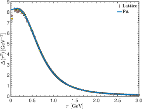
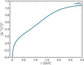
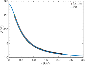
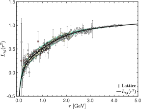
Figure 7: Upper panel: The gluon propagator (left) and the first derivative of its inverse (right). Lower panel: The ghost dressing function (left) and the soft gluon form factor $\mathit{L}_{{sg}}(r^{2})$ of the three-gluon vertex (right). All items are taken from Aguilar et al. (2021a), and have been cured from volume and discretization artifacts. Note that $\mathit{L}_{{sg}}(r^{2})$ is markedly below unity in the infrared, displaying the characteristic zero crossing and the attendant logarithmic divergence at the origin Aguilar et al. (2014a); Athenodorou et al. (2016); Boucaud et al. (2017); Blum et al. (2015); Corell et al. (2018); Aguilar et al. (2019b).

Then, the numerator, ${\cal N}$, and denominator, ${\cal D}$, of the fraction on the r.h.s. of Eq. (75), after employing Eq. (67), become

$${\cal N}=4(d-1)[r^{2}-(r\cdot q)^{2}/q^{2}]{\cal A}_{1}(r^{2})\,,\qquad{\cal D}=4(d-1)[r^{2}-(r\cdot q)^{2}/q^{2}]\,.$$ (76)

At this point, the path-dependent contribution contained in the square bracket drops out when forming the ratio ${\cal N}/{\cal D}$, and Eq. (75) yields the important relation Aguilar et al. (2021a)

$$\mathit{L}_{{sg}}(r^{2})={\cal A}_{1}(r^{2})\,.$$ (77)

In conclusion, the form factor ${\cal A}_{1}(r^{2})$ appearing in Eq. (74) is precisely the one measured on the lattice in the soft-gluon kinematics; Eq. (77) is to be employed in Eq. (74), in order to substitute ${\cal A}_{1}(r^{2})$ by $\mathit{L}_{{sg}}(r^{2})$.

After this last operation, we pass the result of Eq. (74) from Minkowski to Euclidean space, following the standard conversion rules. Specifically, we set $r^{2}=-r_{{\scriptscriptstyle\rm E}}^{2}$, with $r^{2}_{{\scriptscriptstyle\rm E}}>0$ the positive square of an Euclidean four-vector, and use

$$\Delta_{{\scriptscriptstyle\rm E}}(r^{2}_{{\scriptscriptstyle\rm E}})= -\Delta(-r^{2}_{{\scriptscriptstyle\rm E}})\,,\qquad F_{{\scriptscriptstyle\rm E}}(r^{2}_{{\scriptscriptstyle\rm E}})= F(-r^{2}_{{\scriptscriptstyle\rm E}})\,,$$

$$\mathit{L}_{{sg}}^{{\scriptscriptstyle\rm E}}(r^{2}_{{\scriptscriptstyle\rm E}})= \mathit{L}_{{sg}}(-r^{2}_{{\scriptscriptstyle\rm E}})\,,\qquad{\mathbb{C}}_{{\scriptscriptstyle\rm E}}(r^{2}_{{\scriptscriptstyle\rm E}})= -{\mathbb{C}}(-r^{2}_{{\scriptscriptstyle\rm E}})\,.$$ (78)

Then, solving for ${\mathbb{C}}(r^{2})$, we get (suppressing the indices “${\rm E}$”)

$${\mathbb{C}}(r^{2})=\mathit{L}_{{sg}}(r^{2})-F(0)\left\{\frac{{\cal W}(r^{2})}{r^{2}}\Delta^{-1}(r^{2})+\widetilde{Z}_{1}[\Delta^{-1}(r^{2})]^{\prime}\right\}\,.$$ (79)

For the determination of ${\mathbb{C}}(r^{2})$, we use lattice inputs for all the quantities that appear on the r.h.s. of Eq. (79), with the exception of the function ${\cal W}(r^{2})$, which will be computed from the SDE satisfied by the ghost-gluon kernel. The lattice inputs are shown in Fig. 7; all curves are renormalized at $\mu=4.3$ MeV. The computation of ${\cal W}(r^{2})$ is rather technical, and has been given in detail in Aguilar et al. (2022), Appendix B; the result is shown in the left panel of Fig. 8.

When all aforementioned quantities are inserted into the r.h.s. of Eq. (79), a nontrivial result emerges for ${\mathbb{C}}(r^{2})$, which is shown in the right panel of Fig. 8. The blue error band assigned to ${\mathbb{C}}(r^{2})$ represents the total propagation of the individual errors associated with all the inputs entering in Eq. (79). Quite interestingly, the result obtained is not only markedly different from the case ${\mathbb{C}}(r^{2})=0$ (green dotted horizontal line in the right panel of Fig. 8), but it bares a striking resemblance to the ${\mathbb{C}}(r^{2})$ obtained from the BSE solution. In fact, the marked similarity between the two curves provides strong evidence in support of the veracity of the approximations employed in deriving these results, and corroborates the SDE treatment that yields the result for ${\cal W}(r^{2})$ shown in the left panel of Fig. 8.

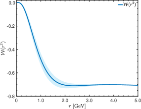
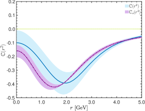
Figure 8: Left panel: The function ${\cal W}(r^{2})$, computed from the one-loop dressed SDE that governs the ghost-gluon kernel. Right panel: The displacement function ${\mathbb{C}}(r^{2})$ obtained from Eq. (79) (blue continuous curve), compared to the same quantity obtained from the BSE in Eq. (25) (purple dot-dashed curve).

IX Ward identity displacement and seagull identity

When deriving the mass formula of Eq. (39) we dealt exclusively with the $q^{\mu}q^{\nu}$ component of gluon propagator, given that the pole terms $V$ contribute only to this particular tensorial structure. Of course, the transversality of the self-energy, as captured by Eq. (4), clearly states that the complete treatment of the $g^{\mu\nu}$ component must yield precisely the same answer; nonetheless, the detailed demonstration of this fact in the present context is highly non-trivial. In particular, the WI displacement turns out to be crucial for the appearance of a term $g^{\mu\nu}\Delta^{-1}(0)$, as can be best exposed within the formalism emerging from the fusion of the pinch technique (PT) Cornwall (1982); Cornwall and Papavassiliou (1989); Pilaftsis (1997); Binosi and Papavassiliou (2002b, 2009) and the BFM, known as “PT-BFM scheme”. In this section we will briefly outline the key elements of this general construction; for further details, the reader is referred to Aguilar and Papavassiliou (2006); Binosi and Papavassiliou (2008a).

(i) Within the PT-BFM framework, the starting point of our analysis is the propagator $\widetilde{\Delta}_{\mu\nu}(q)$ connecting a quantum gluon, $Q^{a}_{\mu}(q)$, with a background one, $B^{a}_{\mu}(-q)$; the corresponding self-energy, $\widetilde{\Pi}_{\mu\nu}(q)$, is diagrammatically shown in Fig. 9. One of the most striking properties of $\widetilde{\Pi}_{\mu\nu}(q)$ is its “block-wise” transversality Aguilar and Papavassiliou (2006); Binosi and Papavassiliou (2008a, b): each of the three subsets of diagrams shown in Fig. 9 is individually transverse, i.e.,

$$q_{\nu}\widetilde{\Pi}_{i}^{\mu\nu}(q)=0\qquad i=1,2,3.$$ (80)

This result is a direct consequence of the Abelian STIs satisfied by the fully dressed vertices, denoted by $\widetilde{{\rm{I}}\!\Gamma}$, entering in these diagrams, namely

$$q^{\mu}\widetilde{{\rm{I}}\!\Gamma}_{\mu\alpha\beta}(q,r,p) = \Delta_{\alpha\beta}^{-1}(r)-\Delta_{\alpha\beta}^{-1}(p)\,,$$

$$q^{\mu}\widetilde{{\rm{I}}\!\Gamma}^{mnrs}_{\mu\alpha\beta\gamma}(q,r,p,t) = f^{mse}f^{ern}{{\rm{I}}\!\Gamma}_{\alpha\beta\gamma}(r,p,q+t)+f^{mne}f^{esr}{{\rm{I}}\!\Gamma}_{\beta\gamma\alpha}(p,t,q+r)$$ (81)

$$+ f^{mre}f^{ens}{{\rm{I}}\!\Gamma}_{\gamma\alpha\beta}(t,r,q+p)\,,$$

together with Eq. (54).

(ii) $\Delta(q^{2})$ and $\widetilde{\Delta}(q^{2})$ are related by the exact identity

$$\Delta(q^{2})=[1+G(q^{2})]\widetilde{\Delta}(q^{2})\,,$$ (82)

where $G(q^{2})$ is the $g_{\mu\nu}$ component of a special two-point function Grassi et al. (2001); Binosi and Papavassiliou (2002a); Binosi and Quadri (2013). Eq. (82) allows one to recast the SDE governing $\Delta(q^{2})$ in the alternative form

$$\Delta^{-1}(q^{2})P_{\mu\nu}(q)=\frac{q^{2}P_{\mu\nu}(q)+i\widetilde{\Pi}_{\mu\nu}(q)}{1+G(q^{2})}\,,$$ (83)

which has the advantage that its diagrammatic expansion contains vertices that satisfy Abelian STIs. Note finally that, in the Landau gauge only, the powerful identity $F^{-1}(0)=1+G(0)$ Aguilar et al. (2009b) expresses the function $G$ at the origin in terms of the saturation value of the ghost dressing function.

(iii) The corresponding vertices develop massless poles, following the exact same pattern indicated in Eqs. (12) and (13). We can set generically,

$$\widetilde{{\rm{I}}\!\Gamma}=\widetilde{\Gamma}+\widetilde{V}\,,$$ (84)

and the tensorial structures of the vertices $\widetilde{V}$ are those given in Eq. (13), but with the corresponding form factors carrying a “tilde”, e.g.,

$$\widetilde{V}_{\alpha}(q,r,p)=\frac{q_{\alpha}}{q^{2}}\widetilde{C}(q,r,p).$$ (85)

(iv) In order to isolate the $g^{\mu\nu}$ component, we simply set $q=0$ in the parts of the diagrams that contain the pole-free vertices, $\widetilde{\Gamma}$; the implementation of this limit, in turn, triggers the corresponding WIs. The block-wise transversality property of Eq. (80) enables one to meaningfully consider this limit within each block, in the sense that there is no communication between blocks that enforces cancellations, as happens in the conventional formulation within the ordinary covariant gauges. We can therefore illustrate the basic point by means of the block that is operationally simpler, namely $\widetilde{\Pi}_{2}^{\mu\nu}(q)$, composed by diagrams $a_{3}$ and $a_{4}$ of Fig. 9.

(v) A crucial ingredient in this demonstration is the seagull identity Aguilar and Papavassiliou (2010); Aguilar et al. (2016b), which states that

$$\int\!\!d^{d}k\,k^{2}\frac{\partial f(k^{2})}{\partial k^{2}}+\frac{d}{2}\int\!\!d^{d}k\,f(k^{2})=0\,,$$ (86)

for functions $f(k^{2})$ that satisfy Wilson’s criterion Wilson (1973); the cases of physical interest are $f(k^{2})=\Delta(k^{2}),D(k^{2})$. This identity is particularly powerful, because, in conjunctions with the WIs of the PT-BFM formalism, it enforces the nonperturbative masslessness of the gluon in the absence of the Schwinger mechanism.

(vi) We now want to determine the value of the $g^{\mu\nu}$ component of $\widetilde{\Pi}_{2}^{\mu\nu}(q)$ at $q=0$. We have that the ($q$-independent) contribution from $a^{\mu\nu}_{4}$ is proportional to $g^{\mu\nu}$, while $a_{3}^{\mu\nu}(q)$ contains both $g^{\mu\nu}$ and $q^{\mu}q^{\nu}$ components; however, in the limit $q\to 0$ the latter vanish, precisely due to the absence of a pole in $q^{2}$. Let us denote by ${\cal B}(q^{2})$ the total contribution proportional to $g^{\mu\nu}$ originating from both diagrams; using the Feynman rules of the BFM Binosi and Papavassiliou (2009), it is rather straightforward to show that, as $q\to 0$,

$$i{\cal B}(0)=\frac{2\lambda}{d}F(0)\left[\int_{k}k_{\mu}D^{2}(k^{2})\widetilde{\Gamma}^{\mu}(0,-k,k)-d\int_{k}D(k^{2})\right]\,.$$ (87)

When the Schwinger mechanism is turned off, the WI of Eq. (50) may be recast in the form

$$\widetilde{\Gamma}^{\mu}(0,-k,k)=-2k^{\mu}D^{-2}(k^{2})\frac{\partial D(k^{2})}{\partial k^{2}}\,,$$ (88)

and so Eq. (87) becomes

$$i{\cal B}(0)=-\frac{4\lambda}{d}F(0)\underbrace{\left[\int_{k}k^{2}\frac{\partial D(k^{2})}{\partial k^{2}}+\frac{d}{2}\int_{k}D(k^{2})\right]}_{\rm seagull\,\,identity}=0\,.$$ (89)

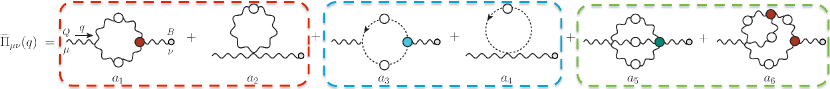
Figure 9: The diagrammatic representation of the self-energy $\widetilde{\Pi}_{\mu\nu}(q)$; the grey circles at the end of the gluon lines indicate a background gluon. The corresponding Feynman rules are given in the Appendix B of Binosi and Papavassiliou (2009).

When the Schwinger mechanism is activated, the displaced WI of Eq. (58) must be employed, such that

$$\widetilde{\Gamma}^{\mu}(0,-k,k)=-2k^{\mu}\left[D^{-2}(k^{2})\frac{\partial D(k^{2})}{\partial k^{2}}+\widetilde{\cal C}(k^{2})\right]\,.$$ (90)

Upon insertion of Eq. (90) into Eq. (87), the first term triggers the seagull identity as before and vanishes, while the second furnishes a nonvanishing finite result

$$i{\cal B}(0)=\frac{4\lambda}{d}F(0)\int_{k}k^{2}D^{2}(k^{2})\widetilde{\cal C}(k^{2})\,.$$ (91)

(vii) Using the exact relation Aguilar et al. (2022)

$${\mathcal{C}}(k^{2})=F(0)\,{\widetilde{\mathcal{C}}}(k^{2})\,,$$ (92)

which is derived from the “background-quantum identity” that relates $\widetilde{\rm{I}}\!\Gamma_{\alpha}(q,r,p)$ and ${\rm{I}}\!\Gamma_{\alpha}(q,r,p)$ Binosi and Papavassiliou (2002a, 2009), Eq. (91) becomes

$$i{\cal B}(0)=\frac{4\lambda}{d}\int_{k}k^{2}D^{2}(k^{2}){\mathcal{C}}(k^{2})\,.$$ (93)

Setting $d=4$, introducing the renormalization constant $\widetilde{Z}_{1}$ and the ghost dressing function $F$, then passing to Euclidean space and employing spherical coordinates, it is straightforward to confirm that the expression in Eq. (93) is identical to that given by the second term in Eq. (39). Completely analogous procedures may be applied to the remaining two blocks, $\widetilde{\Pi}_{1}^{\mu\nu}(q)$ and $\widetilde{\Pi}_{3}^{\mu\nu}(q)$, by exploiting the Abelian STIs of Eq. (81) Binosi et al. (2012).

In summary, the WI displacement of the vertices evades the seagull identity, and endows the $g^{\mu\nu}$ component of the gluon propagator with the exact amount of mass required by its transverse nature.

X Relating the gluon mass with the transition amplitude

It is particularly instructive to zoom into the detailed composition of the vertex $V_{\alpha\mu\nu}(q,r,p)$, by essentially unfolding the black circles in Fig. 2 and exposing the diagrammatic structure of the transition amplitude $I_{\alpha}(q)$, introduced in the paragraph following Eq. (14). This analysis unravels interesting diagrammatic properties, and allows us to derive a simple relation between the transition amplitude and the gluon mass.

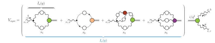
Figure 10: The diagrammatic representation of the vertex $V_{\alpha\mu\nu}(q,r,p)$ in terms of the transition amplitude $I_{\alpha}(q)$, the propagator of the massless excitation, and the vertex function. Note that the diagrams $s_{i}$ are in one-to-one correspondence with the $d_{i}$ of Fig. 1, except for the seagull graph $d_{2}$, which has no analogue $s_{2}$.

The basic elements composing the vertex $V_{\alpha\mu\nu}(q,r,p)$, shown in Fig. 10, are: (i) the transition amplitude $I_{\alpha}(q)$, which connects a gluon to the massless composite excitation, (ii) the propagator of the latter, and (iii) the vertex function $B_{\mu\nu}(q,r,p)$, connecting the massless excitation to a pair of gluons. Since color indices are suppressed in Fig. 10, we emphasize that the propagator of the colored massless excitations is given by the expression $i\delta^{ab}/q^{2}$, i.e., it carries color, as it should. Similarly, the vertex $B_{\mu\nu}(q,r,p)$ is multiplied by the structure constants $f^{abc}$, providing precisely the color term that has been factored out from $V_{\alpha\mu\nu}(q,r,p)$ in Eq. (13). Thus, we have

$$V_{\alpha\mu\nu}(q,r,p)=I_{\alpha}(q)\left(\frac{i}{q^{2}}\right)B_{\mu\nu}(q,r,p)\,,\qquad I_{\alpha}(q)=q_{\alpha}I(q^{2})\,,$$ (94)

with

$$B_{\mu\nu}(q,r,p)=B_{1}\,g_{\mu\nu}+B_{2}\,r_{\mu}r_{\nu}+B_{3}\,p_{\mu}p_{\nu}+B_{4}\,r_{\mu}p_{\nu}+B_{5}\,p_{\mu}r_{\nu}\,.$$ (95)

Given that the $V_{\alpha\mu\nu}(q,r,p)$ appearing in Eqs. (13) and (94) represents the same vertex, we deduce immediately that

$$C_{1}(q,r,p)=iI(q^{2})B_{1}(q,r,p)\,.$$ (96)

Evidently, since $C_{1}(0,r,-r)=0$ [see Eqs. (20) and (70)], one obtains from Eq. (96) that $B_{1}(0,r,-r)=0$, so that

$$\lim_{q\to 0}{B}_{1}(q,r,p)=2(q\cdot r){\mathbb{B}}(r^{2})+\cdots\,,\qquad{\mathbb{B}}(r^{2}):=\left[\frac{\partial{B}_{1}(q,r,p)}{\partial p^{2}}\right]_{q=0}\,,$$ (97)

and therefore, from Eq. (96) we have

$${\mathbb{C}}(r^{2})=iI(0){\mathbb{B}}(r^{2})\,.$$ (98)

In order to illustrate the origin of a key relation between $I(0)$ and $m^{2}$, let us simplify the discussion by assuming that graph $s_{1}$ in Fig. 10 represents the only contribution to $I^{\alpha}(q)$, to be denoted by ${\bar{I}}^{\alpha}(q)$. Clearly, the equivalent approximation at the level of the analysis presented in Sec. V would be to assume that only graph $d_{1}$ in Fig. 1 contributes to the gluon mass.

It is straightforward to deduce from Fig. 10 that ${\bar{I}}^{\alpha}(q)$ is given by

$${\bar{I}}^{\alpha}(q)=\frac{C_{A}}{2}\int_{k}\Gamma_{0}^{\alpha\beta\lambda}(-q,-k,k+q)\Delta_{\lambda\mu}(k)\Delta_{\beta\nu}(k+q)B^{\mu\nu}(q,k,-k-q)\,,$$ (99)

where $\frac{1}{2}$ is the corresponding symmetry factor. Since, by Lorentz invariance, ${\bar{I}}^{\alpha}(q)=q^{\alpha}{\bar{I}}(q^{2})$, we have that ${\bar{I}}(q^{2})=q_{\alpha}{\bar{I}}^{\alpha}(q)/q^{2}$. Therefore, from Eq. (99) we obtain

$${\bar{I}}(q^{2})=\frac{C_{A}}{2\,q^{2}}\int_{k}\{q_{\alpha}\Gamma_{0}^{\alpha\beta\lambda}(-q,-k,k+q)\}\Delta_{\lambda\mu}(k)\Delta_{\beta\nu}(k+q)B^{\mu\nu}(-q,-k,k+q)\,.$$ (100)

Next, employing the expression for $\Gamma_{\!0}^{\alpha\mu\nu}(q,r,p)$ given in Eq. (14), we have that

$$q_{\alpha}\Gamma_{0}^{\alpha\beta\lambda}(q,k,-k-q)=-(q^{2}+2q\cdot k)g^{\beta\lambda}+\cdots$$ (101)

where the ellipsis indicates terms that get annihilated upon contraction with the Landau-gauge propagators $\Delta_{\lambda\mu}(k)$ and $\Delta_{\beta\nu}(k+q)$ in the integrand of Eq. (100).

In order to determine from Eq. (100) the expression for ${\bar{I}}(0)$, note that, by virtue of Eq. (97), only the term $(2q\cdot k)$ in Eq. (101) contributes to ${\bar{I}}(0)$, yielding the combined contribution $(2q\cdot k)^{2}\,{\mathbb{B}}(k^{2})$. Thus, using that $P_{\mu}^{\mu}(k)=3$,

$${\bar{I}}(0) = -6C_{A}\frac{q^{\mu}q^{\nu}}{q^{2}}\int_{k}k_{\mu}k_{\nu}\Delta^{2}(k^{2}){\mathbb{B}}(k^{2})$$ (102)

$$= -\frac{3C_{A}}{2}\int_{k}k^{2}\Delta^{2}(k^{2}){\mathbb{B}}(k^{2})\,.$$

Returning to Eq. (33), and substituting in it Eq. (98), it is clear that ($\lambda:=ig^{2}C_{\rm A}/2$)

$$i{\widehat{d}}_{1}(0)=g^{2}{\bar{I}}(0)\underbrace{\left\{-\frac{3C_{A}}{2}\int_{k}k^{2}\Delta^{2}(k^{2}){\mathbb{B}}(k^{2})\right\}}_{\bar{I}(0)}\,.$$ (103)

As mentioned above, at this level of approximation, $i{\widehat{d}}_{1}(0)$ is the only contribution to the gluon mass, to be denoted by ${\overline{m}}^{2}$; so, Eq. (103) becomes

$${\overline{m}}^{2}=g^{2}{\bar{I}}^{2}(0)\,.$$ (104)

Thus, the pattern that emerges from the study of this particular example may be summarized as follows: when the vertex $V_{\alpha\mu\nu}$ is given by Eq. (94) with $I_{\alpha}(q)\to{\bar{I}}_{\alpha}(q)$, its insertion in the corresponding propagator graph $d_{1}$ leads to the replication of the ${\bar{I}}_{\alpha}(q)$, as shown schematically in Fig. 11.

It turns out that this property may be generalized to include the entire $I_{\alpha}(q)$, composed by the graphs $s_{1}$, $s_{3}$, $s_{4}$, and $s_{5}$ in Fig. 10, provided that the propagator graphs $d_{1}$, $d_{3}$, $d_{4}$, and $d_{5}$ of Fig. 1 are correspondingly included; for details, see Ibañez and Papavassiliou (2013). The final result is precisely the generalization of Eq. (104), namely

$$m^{2}=g^{2}I^{2}(0)\,.$$ (105)

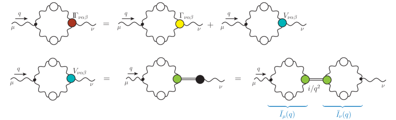
Figure 11: The diagrammatic representation of the sequence that leads to Eq. (104). First row: The diagram $d_{1}$ of Fig. 1, once the replacement ${\rm{I}}\!\Gamma_{\alpha\mu\nu}(q,r,p)=\Gamma_{\alpha\mu\nu}(q,r,p)+V_{\alpha\mu\nu}(q,r,p)$ of Eq. (12) has been implemented. Second row: The diagrammatic steps that leads to the replication of the ${\bar{I}}_{\alpha}(q)$, and eventually to Eq. (104).

We emphasize that, as far as the numerical determination of the gluon mass is concerned, Eq. (105) contains the same information as Eq. (39), once the diagrammatic expansion of $I_{\alpha}(q)$ has been implemented. Nonetheless, the formulation presented above exposes an elaborate diagrammatic pattern, and is particularly useful for the analysis presented in the next section, mainly due to the role played by the vertex function $B_{\mu\nu}(q,r,p)$.

XI Absence of pole divergences in the $S$-matrix

As has been emphasized in the early literature on the subject, one of the main properties of the massless composite excitations that trigger the Schwinger mechanism is that they do not induce divergences in on-shell amplitudes, see, e.g.,  Jackiw and Johnson (1973); Jackiw (1973). In the case of the Yang-Mills theories that we study, the elimination of potentially divergent terms hinges on the longitudinality of the vertices $V$, as captured by Eq. (13), in conjunction with the special limit given by Eq. (97). In this section we demonstrate with a specific example how all terms containing massless poles are either annihilated in their entirety, or, in the kinematic limit where poles might in principle cause divergences, they actually give finite contributions, i.e., they correspond to evitable singularities.

Let us consider the elastic scattering process $g_{\mu}^{a}(k_{1})g_{\nu}^{b}(k_{2})\to g_{\rho}^{c}(k_{3})g_{\sigma}^{d}(k_{4})$, depicted in Fig. 12, where the $g_{\alpha}^{a}(k_{i})$ denotes an “on-shell” gluon of momentum $k_{i}$, and $q=k_{2}-k_{1}=k_{4}-k_{3}$ is the corresponding momentum transfer, with $q^{2}=t$ is the relevant Mandelstam variable. The scattering amplitude consists of the three distinct terms denoted by ($a$), ($b$), and ($c$) in Fig. 12. We notice that, unlike ($a$) and ($c$), diagram ($b$) has no perturbative analogue, since all components that comprise it are generated through nonperturbative effects; observe, in particular, the appearance of the vertex function $B_{\mu\nu}(q,r,p)$, introduced in the previous section.

As we will show at the end of this section, the elimination of all pole divergences does not rely on any particular properties associated with the “on-shellness” of the gluons; this feature is especially welcome, given that gluons do not appear as asymptotic states. Nonetheless, it is instructive to first examine how the cancellations proceed when the gluons are assumed to be on shell, because this will allow us to identify the crucial properties that must be fulfilled in the off-shell case.

To that end, let us assume that, due to the on-shellness of the gluons, each external leg is contracted by the corresponding transverse polarization vector, $\epsilon^{\mu}(k)$, for which

$$k^{\mu}\epsilon_{\mu}(k)=0\,.$$ (106)

We start our discussion with diagram $(a)$, given by

$$(a)=\epsilon^{\mu}(k_{1})\epsilon^{\nu}(k_{2}){\rm{I}}\!\Gamma^{\alpha\mu\nu}(q,k_{1},k_{2})\Delta(q)P^{\alpha\beta}(q){\rm{I}}\!\Gamma^{\beta\rho\sigma}(q,k_{3},k_{4})\epsilon^{\rho}(k_{3})\epsilon^{\sigma}(k_{4})\,.$$ (107)

Noting that, due to the longitudinality of $V_{\alpha\mu\nu}(q,r,p)$,

$$V_{\alpha\mu\nu}(q,r,p)P^{\alpha\beta}(q)\epsilon^{\mu}(r)\epsilon^{\nu}(p)=0\,,$$ (108)

it is clear that the terms $V$ drop out from Eq. (107), and the two fully dressed vertices ${\rm{I}}\!\Gamma$ are replaced by their pole-free counterparts, $\Gamma$. As a result, the contribution from graph ($a$) is finite.

Turning to diagram ($b$), we have that

$$(b)=B_{\mu\nu}(q,k_{1},k_{2})\left[\frac{i}{q^{2}}\right]B_{\rho\sigma}(q,k_{3},k_{4})\,.$$ (109)

As the limit $q\to 0$ is taken, Eq. (97) is triggered, such that

$$\lim_{q\to 0}\,(b) = \{2(q\cdot k_{1})\,{\mathbb{B}}(k_{1}^{2})\}\left[\frac{i}{q^{2}}\right]\{2(q\cdot k_{3})\,{\mathbb{B}}(k_{3}^{2})\}$$ (110)

$$= 4i\lvert k_{1}\rvert\lvert k_{3}\rvert\cos\theta_{1}\cos\theta_{3}\,{\mathbb{B}}(k_{1}^{2})\,{\mathbb{B}}(k_{3}^{2})\,,$$

where $\theta_{1}$ and $\theta_{3}$ are the angles formed between $q$ and $k_{1}$ and $k_{3}$, respectively. The above contribution is clearly finite.

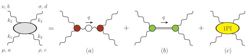
Figure 12: The four-gluon scattering amplitude and the three types of diagrams contributing to it. The abbreviation “1PI” stands for “one-particle irreducible”. Note that diagram ($b$) is composed entirely by nonperturbative structures.

Finally, note that none of the possible $V$-type vertices survives in the diagrams contributing to ($c$), precisely due to their longitudinal nature. Indeed, if a vertex is fully inserted in a diagram, i.e., when none of its momenta is any of the $k_{i}$, then it is contracted by three Landau-gauge gluon propagators, and Eq. (15) is automatically triggered. If, on the other hand, some of the legs of the vertex carry a momentum $k_{i}$, say $k_{1}$, then the part of $V$ that does not get cancelled by the transverse gluon propagators will necessary be proportional to $k_{1}^{\mu}/k^{2}$; it is therefore annihilated upon contraction with the $\epsilon_{\mu}(k_{1})$, by virtue of Eq. (106).

Thus, it is evident from the above considerations that, in the limit $q\to 0$, the terms associated with the massless composite excitations furnish only finite contributions to the amplitude.

It is important to recognize that, in the above demonstration, the only element introduced due to the assumed on-shellness of the scattered gluons is the contraction of the amplitude by the corresponding polarization vectors, satisfying Eq. (106). In particular, note that at no point have we assumed anything special about the values of $k_{i}^{2}$, i.e., neither that $k_{i}^{2}=0$ nor that $k_{i}^{2}=m^{2}$.

As a result, it is possible to relax the on-shellness condition completely, and consider the above amplitude as an off-shell sub-process, embedded into a more complicated scattering process, as depicted in Fig. 13. Indeed, the demonstration presented above goes through unaltered, because the on-shell gluons are replaced by Landau-gauge propagators, which trigger precisely the same relations that the polarization vectors did in the on-shell case.

In conclusion, the above analysis, albeit restricted to a special example, strongly supports the notion that the terms associated with the massless excitations do not induce any divergences in the QCD scattering amplitudes.

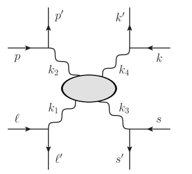
Figure 13: The four-gluon amplitude regarded as a completely off-shell subprocess, embedded into a multi-quark scattering process.

XII Conclusions

The apparent simplicity of the QCD Lagrangian conceals an enormous wealth of dynamical patterns, giving rise to a vast array of complex “emergent phenomena” Roberts and Mezrag (2017). As has been argued in a series of recent works Roberts (2020, 2021); Binosi (2022), the pivotal notion that unifies all these phenomena is the emergence of a hadronic mass, which leaves its imprint on a wide range of physical observables. The generation of a mass scale due to the self-interactions of the gluons represents arguably the most fundamental expression of such an emergence. In the present work we have highlighted certain salient aspects of the research activity dedicated to this subject, within a framework that is based predominantly on the SDEs of the theory, but capitalizes extensively on a number of results obtained from large-volume lattice simulations.

The central idea underlying the approach summarized in this article is the implementation of the celebrated Schwinger mechanism in the context of nonperturbative QCD. The activation of this mechanism hinges on the formation of massless longitudinal poles in the fundamental vertices of the theory. These poles are composite and carry color, and play a dual role: they provide the required structures in the gluon vacuum polarization, and affect nontrivially the way that the STIs of these vertices are realized. This dual nature of the poles is perfectly encoded in the function ${\mathbb{C}}(r^{2})$, which describes the distinct displacement to the WI satisfied by the pole-free part of the three-gluon vertex, and, at the same time, is the bound-state wave function that governs the dynamical formation of the massless poles by the merging of two gluons, through a characteristic BSE. This duality, in turn, unveils a profound connection between dynamics (BSEs) and symmetry (STIs), which becomes particularly patent within the PT-BFM framework.

In fact, it is especially tempting to interpret these massless poles as composite would-be Nambu-Goldstone bosons, given that they appear to fulfill precisely all crucial functions typically ascribed to the latter, namely (i) they are “absorbed” by the gluons to make them massive, (ii) maintain the STIs of the theory intact once the gluons have been endowed with mass, (iii) are longitudinally coupled, and (iv) do not introduce divergences in physical observables, e.g., the $S$-matrix, as was shown in Sec. XI. It would be clearly interesting to pursue this point further; a most promising starting point for such an investigation is offered by the PT-based analysis first presented in Papavassiliou (1990).

The displacement of the WI, quantified by the function ${\mathbb{C}}(r^{2})$, is exclusive to the special realization of the Schwinger mechanism reviewed here. The use of lattice results for the main ingredients entering in the pertinent WI reveals the presence of a robust model-independent signal for ${\mathbb{C}}(r^{2})$, which is in agreement with the result obtained for it from the solution of the BSE, under certain simplifying assumptions. These findings corroborate the operation of the Schwinger mechanism in QCD, and set the stage for further novel developments.

References

- Marciano and Pagels (1978) W. J. Marciano and H. Pagels, Phys. Rept. 36, 137 (1978).
- Collins (1986) J. C. Collins, Renormalization: An Introduction to Renormalization, The Renormalization Group, and the Operator Product Expansion, Cambridge Monographs on Mathematical Physics, Vol. 26 (Cambridge University Press, Cambridge, 1986).
- Cloet and Roberts (2014) I. C. Cloet and C. D. Roberts, Prog. Part. Nucl. Phys. 77, 1 (2014).
- Aguilar et al. (2016a) A. C. Aguilar, D. Binosi, and J. Papavassiliou, Front. Phys.(Beijing) 11, 111203 (2016a).
- Roberts (2020) C. D. Roberts, Symmetry 12, 1468 (2020).
- Roberts (2021) C. D. Roberts, AAPPS Bull. 31, 6 (2021).
- Horak et al. (2022) J. Horak, F. Ihssen, J. Papavassiliou, J. M. Pawlowski, A. Weber, and C. Wetterich, [arXiv:2201.09747 [hep-ph]] .
- Cornwall (1979) J. M. Cornwall, Nucl. Phys. B 157, 392 (1979).
- Parisi and Petronzio (1980) G. Parisi and R. Petronzio, Phys. Lett. B 94, 51 (1980).
- Cornwall (1982) J. M. Cornwall, Phys. Rev. D 26, 1453 (1982).
- Bernard (1982) C. W. Bernard, Phys. Lett. B 108, 431 (1982).
- Bernard (1983) C. W. Bernard, Nucl. Phys. B 219, 341 (1983).
- Donoghue (1984) J. F. Donoghue, Phys. Rev. D 29, 2559 (1984).
- Mandula and Ogilvie (1987) J. Mandula and M. Ogilvie, Phys. Lett. B 185, 127 (1987).
- Cornwall and Papavassiliou (1989) J. M. Cornwall and J. Papavassiliou, Phys. Rev. D 40, 3474 (1989).
- Wilson et al. (1994) K. G. Wilson, T. S. Walhout, A. Harindranath, W.-M. Zhang, R. J. Perry, and S. D. Glazek, Phys. Rev. D49, 6720 (1994).
- Lavelle (1991) M. Lavelle, Phys. Rev. D 44, 26 (1991).
- Halzen et al. (1993) F. Halzen, G. I. Krein, and A. A. Natale, Phys. Rev. D 47, 295 (1993).
- Mihara and Natale (2000) A. Mihara and A. A. Natale, Phys. Lett. B 482, 378 (2000).
- Philipsen (2002) O. Philipsen, Nucl. Phys. B628, 167 (2002).
- Kondo (2001) K.-I. Kondo, Phys. Lett. B 514, 335 (2001).
- Aguilar et al. (2003) A. C. Aguilar, A. A. Natale, and P. S. Rodrigues da Silva, Phys. Rev. Lett. 90, 152001 (2003).
- Athenodorou and Teper (2020) A. Athenodorou and M. Teper, JHEP 11, 172 (2020).
- Athenodorou and Teper (2021) A. Athenodorou and M. Teper, JHEP 12, 082 (2021).
- Collins et al. (1977) J. C. Collins, A. Duncan, and S. D. Joglekar, Phys. Rev. D 16, 438 (1977).
- Brodsky and Shrock (2008) S. J. Brodsky and R. Shrock, Phys. Lett. B666, 95 (2008).
- Braun et al. (2010) J. Braun, H. Gies, and J. M. Pawlowski, Phys. Lett. B684, 262 (2010).
- Binosi et al. (2015) D. Binosi, L. Chang, J. Papavassiliou, and C. D. Roberts, Phys. Lett. B742, 183 (2015).
- Gao et al. (2018) F. Gao, S.-X. Qin, C. D. Roberts, and J. Rodriguez-Quintero, Phys. Rev. D97, 034010 (2018).
- Binosi and Papavassiliou (2003) D. Binosi and J. Papavassiliou, Nucl. Phys. Proc. Suppl. 121, 281 (2003).
- Aguilar et al. (2009a) A. C. Aguilar, D. Binosi, J. Papavassiliou, and J. Rodriguez-Quintero, Phys. Rev. D80, 085018 (2009a).
- Binosi et al. (2017) D. Binosi, C. Mezrag, J. Papavassiliou, C. D. Roberts, and J. Rodriguez-Quintero, Phys. Rev. D96, 054026 (2017).
- Cui et al. (2020) Z.-F. Cui, J.-L. Zhang, D. Binosi, F. de Soto, C. Mezrag, J. Papavassiliou, C. D. Roberts, J. Rodríguez-Quintero, J. Segovia, and S. Zafeiropoulos, Chin. Phys. C 44, 083102 (2020).
- Cucchieri and Mendes (2007) A. Cucchieri and T. Mendes, PoS LATTICE2007, 297 (2007).
- Cucchieri and Mendes (2008) A. Cucchieri and T. Mendes, Phys. Rev. Lett. 100, 241601 (2008).
- Bogolubsky et al. (2007) I. Bogolubsky, E. Ilgenfritz, M. Muller-Preussker, and A. Sternbeck, PoS LATTICE2007, 290 (2007).
- Bogolubsky et al. (2009) I. Bogolubsky, E. Ilgenfritz, M. Muller-Preussker, and A. Sternbeck, Phys. Lett. B676, 69 (2009).
- Oliveira and Silva (2009) O. Oliveira and P. Silva, PoS LAT2009, 226 (2009).
- Oliveira and Bicudo (2011) O. Oliveira and P. Bicudo, J. Phys. G G38, 045003 (2011).
- Cucchieri and Mendes (2010) A. Cucchieri and T. Mendes, Phys. Rev. D81, 016005 (2010).
- Aguilar et al. (2008) A. C. Aguilar, D. Binosi, and J. Papavassiliou, Phys. Rev. D78, 025010 (2008).
- Fischer et al. (2009) C. S. Fischer, A. Maas, and J. M. Pawlowski, Annals Phys. 324, 2408 (2009).
- Binosi et al. (2012) D. Binosi, D. Ibañez, and J. Papavassiliou, Phys. Rev. D86, 085033 (2012).
- Serreau and Tissier (2012) J. Serreau and M. Tissier, Phys. Lett. B712, 97 (2012).
- Tissier and Wschebor (2010) M. Tissier and N. Wschebor, Phys. Rev. D 82, 101701 (2010).
- Aguilar et al. (2016b) A. C. Aguilar, D. Binosi, C. T. Figueiredo, and J. Papavassiliou, Phys. Rev. D94, 045002 (2016b).
- Peláez et al. (2014) M. Peláez, M. Tissier, and N. Wschebor, Phys. Rev. D 90, 065031 (2014).
- Dudal et al. (2008) D. Dudal, J. A. Gracey, S. P. Sorella, N. Vandersickel, and H. Verschelde, Phys. Rev. D78, 065047 (2008).
- Rodriguez-Quintero (2011) J. Rodriguez-Quintero, J. High Energy Phys. 01, 105 (2011).
- Pennington and Wilson (2011) M. R. Pennington and D. J. Wilson, Phys. Rev. D84, 119901 (2011).
- Meyers and Swanson (2014) J. Meyers and E. S. Swanson, Phys. Rev. D90, 045037 (2014).
- Siringo (2016) F. Siringo, Nucl. Phys. B907, 572 (2016).
- Cyrol et al. (2018a) A. K. Cyrol, J. M. Pawlowski, A. Rothkopf, and N. Wink, SciPost Phys. 5, 065 (2018a).
- Cucchieri et al. (2009) A. Cucchieri, T. Mendes, and E. M. S. Santos, Phys. Rev. Lett. 103, 141602 (2009).
- Cucchieri et al. (2010) A. Cucchieri, T. Mendes, G. M. Nakamura, and E. M. S. Santos, PoS FACESQCD, 026 (2010).
- Bicudo et al. (2015) P. Bicudo, D. Binosi, N. Cardoso, O. Oliveira, and P. J. Silva, Phys. Rev. D92, 114514 (2015).
- Epple et al. (2008) D. Epple, H. Reinhardt, W. Schleifenbaum, and A. P. Szczepaniak, Phys. Rev. D77, 085007 (2008).
- Campagnari and Reinhardt (2010) D. R. Campagnari and H. Reinhardt, Phys. Rev. D82, 105021 (2010).
- Aguilar et al. (2017) A. C. Aguilar, D. Binosi, and J. Papavassiliou, Phys. Rev. D95, 034017 (2017).
- Glazek et al. (2017) S. D. Glazek, M. Gómez-Rocha, J. More, and K. Serafin, Phys. Lett. B773, 172 (2017).
- Bowman et al. (2007) P. O. Bowman, U. M. Heller, D. B. Leinweber, M. B. Parappilly, A. Sternbeck, L. von Smekal, A. G. Williams, and J.-b. Zhang, Phys. Rev. D 76, 094505 (2007).
- Kamleh et al. (2007) W. Kamleh, P. O. Bowman, D. B. Leinweber, A. G. Williams, and J. Zhang, Phys. Rev. D76, 094501 (2007).
- Ayala et al. (2012) A. Ayala, A. Bashir, D. Binosi, M. Cristoforetti, and J. Rodriguez-Quintero, Phys. Rev. D86, 074512 (2012).
- Aguilar et al. (2013a) A. C. Aguilar, D. Binosi, and J. Papavassiliou, Phys. Rev. D88, 074010 (2013a).
- Aguilar et al. (2020a) A. C. Aguilar, F. De Soto, M. N. Ferreira, J. Papavassiliou, J. Rodríguez-Quintero, and S. Zafeiropoulos, Eur. Phys. J. C80, 154 (2020a).
- Schwinger (1962a) J. S. Schwinger, Phys. Rev. 125, 397 (1962a).
- Schwinger (1962b) J. S. Schwinger, Phys. Rev. 128, 2425 (1962b).
- Roberts and Williams (1994) C. D. Roberts and A. G. Williams, Prog. Part. Nucl. Phys. 33, 477 (1994).
- Alkofer and von Smekal (2001) R. Alkofer and L. von Smekal, Phys. Rept. 353, 281 (2001).
- Fischer (2006) C. S. Fischer, J. Phys. G 32, R253 (2006).
- Roberts (2008) C. D. Roberts, Prog. Part. Nucl. Phys. 61, 50 (2008).
- Binosi and Papavassiliou (2009) D. Binosi and J. Papavassiliou, Phys. Rept. 479, 1 (2009).
- Huber (2020) M. Q. Huber, Phys. Rept. 879, 1 (2020).
- Pawlowski et al. (2004) J. M. Pawlowski, D. F. Litim, S. Nedelko, and L. von Smekal, Phys. Rev. Lett. 93, 152002 (2004).
- Pawlowski (2007) J. M. Pawlowski, Annals Phys. 322, 2831 (2007).
- Cyrol et al. (2018b) A. K. Cyrol, M. Mitter, J. M. Pawlowski, and N. Strodthoff, Phys. Rev. D97, 054006 (2018b).
- Corell et al. (2018) L. Corell, A. K. Cyrol, M. Mitter, J. M. Pawlowski, and N. Strodthoff, SciPost Phys. 5, 066 (2018).
- Blaizot et al. (2021) J.-P. Blaizot, J. M. Pawlowski, and U. Reinosa, Annals Phys. 431, 168549 (2021).
- Aguilar et al. (2012) A. C. Aguilar, D. Ibanez, V. Mathieu, and J. Papavassiliou, Phys. Rev. D85, 014018 (2012).
- Ibañez and Papavassiliou (2013) D. Ibañez and J. Papavassiliou, Phys. Rev. D87, 034008 (2013).
- Binosi and Papavassiliou (2018) D. Binosi and J. Papavassiliou, Phys. Rev. D97, 054029 (2018).
- Aguilar et al. (2018) A. C. Aguilar, D. Binosi, C. T. Figueiredo, and J. Papavassiliou, Eur. Phys. J. C78, 181 (2018).
- Eichmann et al. (2021) G. Eichmann, J. M. Pawlowski, and J. a. M. Silva, Phys. Rev. D 104, 114016 (2021).
- Cornwall et al. (2010) J. M. Cornwall, J. Papavassiliou, and D. Binosi, The Pinch Technique and its Applications to Non-Abelian Gauge Theories, Vol. 31 (Cambridge University Press, 2010).
- Cucchieri et al. (2006) A. Cucchieri, A. Maas, and T. Mendes, Phys. Rev. D74, 014503 (2006).
- Cucchieri et al. (2008) A. Cucchieri, A. Maas, and T. Mendes, Phys. Rev. D77, 094510 (2008).
- Athenodorou et al. (2016) A. Athenodorou, D. Binosi, P. Boucaud, F. De Soto, J. Papavassiliou, J. Rodriguez-Quintero, and S. Zafeiropoulos, Phys. Lett. B761, 444 (2016).
- Duarte et al. (2016) A. G. Duarte, O. Oliveira, and P. J. Silva, Phys. Rev. D94, 074502 (2016).
- Boucaud et al. (2018) P. Boucaud, F. De Soto, K. Raya, J. Rodríguez-Quintero, and S. Zafeiropoulos, Phys. Rev. D98, 114515 (2018).
- Taylor (1971) J. Taylor, Nucl. Phys. B 33, 436 (1971).
- Slavnov (1972) A. Slavnov, Theor. Math. Phys. 10, 99 (1972).
- Eichten and Feinberg (1974) E. Eichten and F. Feinberg, Phys. Rev. D 10, 3254 (1974).
- Poggio et al. (1975) E. C. Poggio, E. Tomboulis, and S. H. H. Tye, Phys. Rev. D11, 2839 (1975).
- Smit (1974) J. Smit, Phys. Rev. D 10, 2473 (1974).
- Papavassiliou (1990) J. Papavassiliou, Phys. Rev. D 41, 3179 (1990).
- Aguilar et al. (2022) A. C. Aguilar, M. N. Ferreira, and J. Papavassiliou, Phys. Rev. D 105, 014030 (2022).
- Aguilar and Papavassiliou (2006) A. C. Aguilar and J. Papavassiliou, J. High Energy Phys. 12, 012 (2006).
- Kondo (2010) K.-I. Kondo, Prog. Theor. Phys. 122, 1455 (2010).
- Dudal et al. (2012) D. Dudal, O. Oliveira, and J. Rodriguez-Quintero, Phys. Rev. D86, 105005 (2012).
- Aguilar et al. (2013b) A. C. Aguilar, D. Ibañez, and J. Papavassiliou, Phys. Rev. D87, 114020 (2013b).
- Cyrol et al. (2016) A. K. Cyrol, L. Fister, M. Mitter, J. M. Pawlowski, and N. Strodthoff, Phys. Rev. D94, 054005 (2016).
- Aguilar et al. (2021a) A. C. Aguilar, C. O. Ambrósio, F. De Soto, M. N. Ferreira, B. M. Oliveira, J. Papavassiliou, and J. Rodríguez-Quintero, Phys. Rev. D 104, 054028 (2021a).
- Schleifenbaum et al. (2005) W. Schleifenbaum, A. Maas, J. Wambach, and R. Alkofer, Phys. Rev. D 72, 014017 (2005).
- Huber and von Smekal (2013) M. Q. Huber and L. von Smekal, J. High Energy Phys. 04, 149 (2013).
- Huber et al. (2012) M. Q. Huber, A. Maas, and L. von Smekal, J. High Energy Phys. 11, 035 (2012).
- Blum et al. (2014) A. Blum, M. Q. Huber, M. Mitter, and L. von Smekal, Phys. Rev. D89, 061703 (2014).
- Eichmann et al. (2014) G. Eichmann, R. Williams, R. Alkofer, and M. Vujinovic, Phys. Rev. D89, 105014 (2014).
- Williams et al. (2016) R. Williams, C. S. Fischer, and W. Heupel, Phys. Rev. D93, 034026 (2016).
- Papavassiliou et al. (2022) J. Papavassiliou, A. C. Aguilar, and M. N. Ferreira, Supl. Rev. Mex. Fis. 3, 0308112 (2022).
- Aguilar and Papavassiliou (2010) A. C. Aguilar and J. Papavassiliou, Phys. Rev. D81, 034003 (2010).
- Jackiw and Johnson (1973) R. Jackiw and K. Johnson, Phys. Rev. D 8, 2386 (1973).
- Jackiw (1973) R. Jackiw, In *Erice 1973, Proceedings, Laws Of Hadronic Matter*, New York 1975, 225-251 and M I T Cambridge - COO-3069-190 (73,REC.AUG 74) 23p (1973).
- Aguilar et al. (2014a) A. C. Aguilar, D. Binosi, D. Ibañez, and J. Papavassiliou, Phys. Rev. D89, 085008 (2014a).
- Binosi and Papavassiliou (2002a) D. Binosi and J. Papavassiliou, Phys. Rev. D66, 025024 (2002a).
- Hasenfratz and Hasenfratz (1980) A. Hasenfratz and P. Hasenfratz, Phys. Lett. B 93, 165 (1980).
- Alles et al. (1997) B. Alles, D. Henty, H. Panagopoulos, C. Parrinello, C. Pittori, and D. G. Richards, Nucl. Phys. B502, 325 (1997).
- Davydychev et al. (1998) A. I. Davydychev, P. Osland, and O. V. Tarasov, Phys. Rev. D 58, 036007 (1998).
- Boucaud et al. (1998a) P. Boucaud, J. P. Leroy, J. Micheli, O. Pene, and C. Roiesnel, J. High Energy Phys. 10, 017 (1998a).
- Boucaud et al. (1998b) P. Boucaud, J. P. Leroy, J. Micheli, O. Pene, and C. Roiesnel, JHEP 12, 004 (1998b).
- Nakanishi (1969) N. Nakanishi, Prog. Theor. Phys. Suppl. 43, 1 (1969).
- Maris and Roberts (1997) P. Maris and C. D. Roberts, Phys. Rev. C 56, 3369 (1997).
- Blank and Krassnigg (2011) M. Blank and A. Krassnigg, Comput. Phys. Commun. 182, 1391 (2011).
- Aguilar et al. (2014b) A. C. Aguilar, D. Binosi, and J. Papavassiliou, Phys. Rev. D89, 085032 (2014b).
- Boucaud et al. (2009) P. Boucaud, F. De Soto, J. Leroy, A. Le Yaouanc, J. Micheli, et al., Phys. Rev. D79, 014508 (2009).
- von Smekal et al. (2009) L. von Smekal, K. Maltman, and A. Sternbeck, Phys. Lett. B 681, 336 (2009).
- Boucaud et al. (2011) P. Boucaud, D. Dudal, J. Leroy, O. Pene, and J. Rodriguez-Quintero, J. High Energy Phys. 12, 018 (2011).
- Aguilar et al. (2021b) A. C. Aguilar, F. De Soto, M. N. Ferreira, J. Papavassiliou, and J. Rodríguez-Quintero, Phys. Lett. B 818, 136352 (2021b).
- Aguilar et al. (2010) A. C. Aguilar, D. Binosi, and J. Papavassiliou, J. High Energy Phys. 07, 002 (2010).
- Gell-Mann and Low (1954) M. Gell-Mann and F. E. Low, Phys. Rev. 95, 1300 (1954).
- DeWitt (1967) B. S. DeWitt, Phys. Rev. 162, 1195 (1967).
- Honerkamp (1972) J. Honerkamp, Nucl. Phys. B 48, 269 (1972).
- ’t Hooft (1971) G. ’t Hooft, Nucl. Phys. B 35, 167 (1971).
- Kallosh (1974) R. E. Kallosh, Nucl. Phys. B 78, 293 (1974).
- Kluberg-Stern and Zuber (1975) H. Kluberg-Stern and J. B. Zuber, Phys. Rev. D 12, 482 (1975).
- Abbott (1981) L. Abbott, Nucl. Phys. B 185, 189 (1981).
- Shore (1981) G. M. Shore, Annals Phys. 137, 262 (1981).
- Abbott et al. (1983) L. F. Abbott, M. T. Grisaru, and R. K. Schaefer, Nucl. Phys. B 229, 372 (1983).
- Aguilar et al. (2019a) A. C. Aguilar, M. N. Ferreira, C. T. Figueiredo, and J. Papavassiliou, Phys. Rev. D99, 034026 (2019a).
- Aguilar et al. (2020b) A. C. Aguilar, M. N. Ferreira, and J. Papavassiliou, Eur. Phys. J. C 80, 887 (2020b).
- Parrinello (1994) C. Parrinello, Phys. Rev. D50, R4247 (1994).
- Parrinello et al. (1998) C. Parrinello, D. Richards, B. Alles, H. Panagopoulos, and C. Pittori (UKQCD), Nucl. Phys. B Proc. Suppl. 63, 245 (1998).
- Sternbeck et al. (2017) A. Sternbeck, P.-H. Balduf, A. Kizilersu, O. Oliveira, P. J. Silva, J.-I. Skullerud, and A. G. Williams, PoS LATTICE2016, 349 (2017).
- Vujinovic and Mendes (2019) M. Vujinovic and T. Mendes, Phys. Rev. D99, 034501 (2019).
- Boucaud et al. (2017) P. Boucaud, F. De Soto, J. Rodríguez-Quintero, and S. Zafeiropoulos, Phys. Rev. D95, 114503 (2017).
- Blum et al. (2015) A. L. Blum, R. Alkofer, M. Q. Huber, and A. Windisch, Acta Phys. Polon. Supp. 8, 321 (2015).
- Aguilar et al. (2019b) A. C. Aguilar, M. N. Ferreira, C. T. Figueiredo, and J. Papavassiliou, Phys. Rev. D99, 094010 (2019b).
- Pilaftsis (1997) A. Pilaftsis, Nucl. Phys. B 487, 467 (1997).
- Binosi and Papavassiliou (2002b) D. Binosi and J. Papavassiliou, Phys. Rev. D 66, 111901 (2002b).
- Binosi and Papavassiliou (2008a) D. Binosi and J. Papavassiliou, Phys. Rev. D77, 061702 (2008a).
- Binosi and Papavassiliou (2008b) D. Binosi and J. Papavassiliou, J. High Energy Phys. 11, 063 (2008b).
- Grassi et al. (2001) P. A. Grassi, T. Hurth, and M. Steinhauser, Annals Phys. 288, 197 (2001).
- Binosi and Quadri (2013) D. Binosi and A. Quadri, Phys. Rev. D88, 085036 (2013).
- Aguilar et al. (2009b) A. C. Aguilar, D. Binosi, and J. Papavassiliou, J. High Energy Phys. 11, 066 (2009b).
- Wilson (1973) K. G. Wilson, Phys. Rev. D7, 2911 (1973).
- Roberts and Mezrag (2017) C. D. Roberts and C. Mezrag, EPJ Web Conf. 137, 01017 (2017).
- Binosi (2022) D. Binosi, Few Body Syst. 63, 42 (2022).