Quantum corrections to frame-dragging in scattering amplitudes

Abstract

Frame-dragging effect manifests itself as polarization direction rotation when linearly polarized electromagnetic/gravitational wave scatters from a spinning point source through gravitational interactions, an effect also known as the gravitational Faraday rotation. Treating general relativity as an effective field theory, the Faraday rotation angle and its quantum corrections are computed using scattering amplitudes. While the classical rotation angle is universal as expected from the equivalence principle, the quantum corrections are found to be different between electromagnetic and gravitational waves, supporting earlier studies that some formulations of the equivalence principle may need reformulation in the quantum regime.

I Introduction

Quantum gravity is incomplete in the sense that no known theory remains valid at all energy scales. However, it is known that any theory of gravitons (defined as self-interacting massless spin-2 particles) obeying certain physical principles such as unitarity, Lorentz invariance, and locality must reduce to general relativity (GR) at sufficiently low energy or curvature scales [1, 2, 3]. Moreover, GR as a quantum theory is a perfectly valid effective theory which gives consistent predictions below the cutoff scale, where the cutoff is conjectured to be of the order of the Planck mass [4, 5, 6]. Therefore, it is still possible to make definite predictions in quantum gravity which do not depend on the ultraviolet completion of the theory. The aim of this study is probing quantum corrections to frame-dragging, also known as the Lense-Thirring effect.

Frame-dragging is a feature of GR for which its Newtonian counterpart does not exist. Thus, the study of quantum corrections to frame-dragging is a study of quantum GR, which is qualitatively different from studies of quantum effects in Newtonian gravity; the former cannot be faithfully studied from the latter. This makes quantum frame-dragging an interesting subject of study as usual studies of quantum effects focus on phenomena having Newtonian analogs [4, 5, 7, 8, 9, 10, 11].

Frame-dragging is sourced by angular momentum, and localized distribution of angular momentum can be approximated as a point source with spin. Spin effects in quantum GR have already been studied in the literature; as corrections to the metric [12, 13, 14, 15], or as corrections to the potential [16, 17]. However, both the metric and the potential are gauge-dependent quantities in GR, which renders them incomplete as observable effects. Moreover, the spins of the point sources considered in the works were quantum spins having values of $s=1/2$ or $s=1$. There is a conceptual gap between quantum spin (having values $s=1/2,1,3/2,\cdots$) and classical spin, and closure of the gap seems necessary to make connections with potentially realizable experiments; the frame-dragging effect sourced by quantum spins would be too small to have any observable consequences. Fortunately, methods to circumvent both limitations have already been studied in the literature.

The limitation of gauge-dependent quantities can be overcome by studying scattering observables measured at asymptotic infinity, which are free of gauge ambiguities. The approach has already been used to argue breakdown of the equivalence principle in the quantum realm [10, 11, 18, 19]. A scattering observable that is a direct consequence of frame-dragging effect is the gravitational Faraday rotation (GFR), where polarization direction of linearly polarized light (or gravitational wave) is rotated due to the ambient gravitomagnetic field sourced by angular momentum [20, 21, 22, 23, 24, 25, 26, 27, 28]. The rotation angle can also be computed using scattering amplitudes of quantum field theory [29], which makes it an ideal observable for studying quantum frame-dragging.

The conceptual gap between quantum and classical spin has been studied in the context of scattering amplitude approaches to the classical gravitational two-body problem [5, 8, 9, 30, 31, 32, 33, 34]. While it is known that certain classical spin effects can be captured by quantum spins [16, 35, 36, 37, 38], the description fails to capture terms that are affected by identities dependent on spin representations of the spinning particle, such as trace identities. Therefore, higher-spin ($s>2$) particle descriptions are required to capture the full dynamics of classical spinning particles [39, 40, 41, 42, 43], which has met with great success in determining the classical two-body dynamics in GR [39, 40, 44, 45, 43, 46, 47, 48, 49, 50, 51, 52]. In this work the semiclassical Compton amplitude [48], which is defined as the Compton amplitude in the classical spin limit ($s\to\infty$ with $S=s\hbar$ fixed), is used. Note that amplitude computations at tree level [39, 40, 44, 41, 45, 53] and one-loop level [54, 49, 51, 52] with spins in the classical spin limit have been checked against corresponding classical computations, and found to reproduce classical spin dependence to all orders in spin, which can be viewed as evidence for the validity of the approach.

The GFR angle $\alpha$ and its leading quantum corrections at linear order in spin are computed to be

$$\alpha_{X}(b) =\frac{5\pi G^{2}m^{2}(\hat{k}\cdot\vec{a})}{4b^{3}}+c_{X}\frac{G^{2}m\hbar(\hat{k}\cdot\vec{a})}{\pi b^{4}}\,,$$ (1a)

where $$m \vec{a}=\vec{S}/m b \hat{k}=\vec{k}/\omega X=\gamma,h$$ is the mass of the gravitating point source, is its spin-length vector, is the impact parameter, is the propagation direction of the electromagnetic/gravitational wave, and denotes particle species.

$$\begin{aligned} c_{\gamma}&=-\frac{994}{15}+32\log\frac{b}{b_{0}}&&&&\text{photon}\\ c_{h}&=-60+24\log\frac{b}{b_{0}}&&&&\text{graviton}\end{aligned}$$ (1b)

The leading classical term of Eq.(1a) agrees with known geometric optics limit results [20, 28, 29]. Similar to the deflection angle [10, 11, 18, 19], the quantum corrections to the GFR angle differ for different particle species.

In terms of the deflection angle $\theta=\frac{4Gm}{b}(1+{\mathcal{O}}(\frac{Gm}{b}))$, the GFR angle can be written as

$$\begin{aligned} \alpha_{X}(\theta)&=\frac{5\pi}{256}(\hat{k}\cdot\vec{\chi})\,\theta^{3}+\tilde{c}_{X}\frac{m_{\text{Pl}}^{2}}{m^{2}}(\hat{k}\cdot\vec{\chi})\,\theta^{4}\,,\\ \tilde{c}_{X}&=\left\{\begin{aligned} \tilde{c}_{\gamma}&=-\frac{497}{240}-\log\frac{\theta}{\theta_{0}}&&&&\text{photon}\\ \tilde{c}_{h}&=-\frac{15}{8}-\frac{3}{4}\log\frac{\theta}{\theta_{0}}&&&&\text{graviton}\end{aligned}\right.\end{aligned}$$ (2)

where $\vec{\chi}=\vec{S}/Gm^{2}$ is the dimensionless spin parameter and $m_{\text{Pl}}=\sqrt{\hbar/8\pi G}$ is the reduced Planck mass. This expression has the advantage that all quantities on both sides can (in principle) be directly measured at asymptotic infinity, and that ill-definedness of $b$ at the wave-packet scale can be avoided . It would be interesting to study whether measurements at asymptotic infinity open up loopholes that can be used to bypass the known no-go results for experimental observation of quantum gravity effects [56, 57].

II Computation setup

Consider a massive-massless $2\to 2$ scattering $p_{1}k_{2}\to p_{1}^{\prime}k_{2}^{\prime}$, where $p$ denotes massive momenta with mass $m$ and $k$ denotes massless momenta, while $q=k_{2}^{\prime}-k_{2}=p_{1}-p_{1}^{\prime}$ is the transfer momentum. The massive particle has spin $S^{\mu}$, causing GFR on massless particle’s polarization through frame-dragging.

The GFR angle $\alpha$ is obtained from the difference of phase gain between two helicity states of the massless particle. The difference in phase gain is identified with the difference in eikonal phases $\delta$ of helicity-preserving scattering amplitudes [29],

$$\alpha:=-\frac{\delta_{+}-\delta_{-}}{2|h|}\,,$$ (3)

where the eikonal phase $\delta_{\pm}$ is the logarithm of the scattering amplitude in impact parameter space (IPS) [58, 59, 60, 61, 62, 63, 64, 65].

$$\begin{aligned} e^{i\delta_{\pm}}&:=\int\frac{d^{D}q}{(2\pi)^{D}}P(q)\langle p_{1}^{\prime},k_{2}^{\prime}(\pm)|S|p_{1},k_{2}(\pm)\rangle\,,\\ P(q)&=e^{-ib\cdot q}\hat{\delta}[q\cdot(p_{1}+p_{1}^{\prime})]\hat{\delta}[q\cdot(k_{2}+k_{2}^{\prime})]\,.\end{aligned}$$ (4)

Here $\hat{\delta}(x)=2\pi\delta(x)$, and $\pm$ is the massless particle’s helicity. The classical terms of the eikonal phase satisfy exponentiation under the adopted projection condition $P(q)$ [66, 67]. Only the nonanalytic terms of the scattering amplitude contribute to finite $b$ eikonal phase, which are constructible from unitarity-based methods [68, 69, 70].

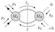
Figure 1: The two-graviton cut for the one-loop amplitude $M_{4}(p_{1},k_{2}^{+h},k_{3}^{-h},p_{4})$. Solid lines denote massive semiclassical spinning particle, dashed lines denote massless helicity $h$ particle, and wavy lines denote internal exchanged gravitons. $M_{L}$ is the semiclassical gravitational spinning Compton amplitude [Eq.(6)], and $M_{R}$ is the two-graviton–two-helicity-$h$ amplitude [Eq.(7)]. Figure drawn with package TikZ-Feynman [71].

The relevant $S$-matrix elements $iM$ can be obtained from the $4\to 0$ amplitude $M_{4}(p_{1},k_{2}^{+h},k_{3}^{-h},p_{4})$ using crossing symmetry. The relevant tree-level amplitudes were found to not contribute to GFR [29],

$$\begin{aligned} M_{4}^{(0)}&=M_{4,s=0}^{(0)}\times\exp\left(\frac{i[{2}|A|{3}\rangle}{[{2}|p_{1}|{3}\rangle}\right)\,,\\ \frac{M_{4,s=0}^{(0)}}{(\kappa/2)^{2}}&=\left\{\begin{aligned} &\phantom{a}-\frac{[{2}|p_{1}|{3}\rangle^{2}}{t}&&h=1\\ &\frac{[{2}|p_{1}|{3}\rangle^{4}}{(s-m^{2})(u-m^{2})t}&&h=2\end{aligned}\right.\end{aligned}$$ (5)

where $s=(p_{1}+k_{2})^{2}$, $t=(k_{2}+k_{3})^{2}$, $u=(p_{1}+k_{3})^{2}$, and $\kappa=\sqrt{32\pi G}$. The case $h=2$ corresponds to the semiclassical spinning Compton amplitude for Kerr black holes valid to quartic order in spin [39, 44, 72, 42, 48], which also enters the two-graviton cut in Fig.1 as $M_{L}$. The vector $A^{\mu}=(k_{2}+k_{3})_{\nu}S^{\mu\nu}(p_{1})$ was introduced to simplify the notations . The spin tensor $S^{\mu\nu}(p_{1})$ is the Lorentz generator $J^{\mu\nu}$ restricted to the little group space of the incoming particle of momentum $p_{1}$, satisfying the covariant spin supplementary condition $p_{1\mu}S^{\mu\nu}=0$  and related to the spin vector by $S^{\mu\nu}=-\frac{1}{m}\epsilon^{\mu\nu\alpha\beta}p_{1\alpha}S_{\beta}$. The spin vector is the mass rescaled Pauli-Lubanski pseudovector $S^{\mu}=\frac{-1}{2m}\epsilon^{\mu\alpha\beta\gamma}p_{1\alpha}J_{\beta\gamma}$ [43, 46, 48]. Only the terms up to linear order in spin are considered, but the extension to higher orders would be straightforward.

The relevant terms of the one-loop amplitude $M_{4}^{(1)}$ can be constructed from the two-graviton cut in Fig.1. The cut has nonvanishing contributions only when internal graviton states have opposite helicities [11], e.g. $\ell^{+}$ and $\ell_{1}^{+}$. For this helicity configuration the subamplitudes are given as 

$$M_{L}^{\ell^{+},-\ell_{1}^{-}} =\frac{\left(-{\kappa}/{2}\right)^{2}[{\ell}|p_{1}|{\ell_{1}}\rangle^{4}}{-4t(k_{2}\cdot\ell)(k_{2}\cdot\ell_{1})}\exp\left(\frac{i[{\ell}|A|{\ell_{1}}\rangle}{[{\ell}|p_{1}|{\ell_{1}}\rangle}\right)\,,$$ (6)

$$M_{R}^{-\ell^{-},\ell_{1}^{+}} =\frac{\left(-{\kappa}/{2}\right)^{2}[{\ell_{1}}|2|{\ell}\rangle^{4}}{-4t(k_{2}\cdot\ell)(k_{2}\cdot\ell_{1})}\left(\frac{\langle 3\ell\rangle}{\langle 2\ell\rangle}\right)^{2h}\,,$$ (7)

where $M_{L}=M_{\text{Comp}}(p_{1},\ell^{+2},-\ell_{1}^{-2},p_{4})$ is the semiclassical spinning Compton amplitude Eq.(5), and $M_{R}=M_{XhhX}(k_{2}^{+h},\ell_{1}^{+2},-\ell^{-2},k_{3}^{-h})$ is the two-graviton–two-helicity $h$ amplitude valid for $h\leq 2$. The cases $h=1,2$ are considered, which correspond to the Einstein-Maxwell theory ($h=1$) and GR ($h=2$).

Using unitarity-based methods [68, 69, 70], the one-loop integrand for $M_{4}(p_{1},k_{2}^{+h},k_{3}^{-h},p_{4})$ is constructed from the two-graviton cut as 

$$iM_{4}^{(1)} =\int\hskip-4.0pt\frac{d^{D}\ell}{(2\pi)^{D}}\frac{\left[M_{L}^{\ell^{+},-\ell_{1}^{-}}\hskip-2.0ptM_{R}^{-\ell^{-},\ell_{1}^{+}}\right]+(\ell\leftrightarrow-\ell_{1})}{2\ell^{2}\ell_{1}^{2}}\,,$$ (8)

where the “numerator” $M_{L}\times M_{R}$ captures all momentum dependence of the full one-loop integrand subject to the cut conditions $\ell^{2}=0$ and $\ell_{1}^{2}=(\ell-k_{2}-k_{3})^{2}=0$, which determines the nonanalytic $t$ dependence of the full amplitude relevant to long-distance physics [9]. The second term $(\ell\leftrightarrow-\ell_{1})$ in the numerator of Eq.(8) denotes opposite helicity configuration for the gravitons. Explicit evaluation of the first term $M_{L}^{\ell^{+},-\ell_{1}^{-}}M_{R}^{-\ell^{-},\ell_{1}^{+}}$ for $n$th order in spin yields

$$\begin{aligned} \left.\frac{M_{L}M_{R}}{(\kappa/4)^{4}}\right|_{{\mathcal{O}}(S^{n})}\hskip-9.0pt&=\frac{i^{n}}{n!}\frac{[\text{tr}_{-}(\not{k_{2}}\not{\ell_{1}}\not{p_{1}}\not{\ell})]^{4-n}[\text{tr}_{-}(\not{k_{2}}\not{\ell_{1}}\not{A}\not{\ell})]^{n}}{t^{2}(p_{1}\cdot\ell)(p_{1}\cdot\ell_{1})(k_{2}\cdot\ell)(k_{2}\cdot\ell_{1})}\\ &\phantom{=a}\times\frac{1}{[{3}|p_{1}|{2}\rangle^{2h}}\left(\frac{\text{tr}_{-}(\not{k_{2}}\not{\ell}\not{k_{3}}\not{p_{1}})}{2(k_{2}\cdot\ell)}\right)^{2h}\,,\end{aligned}$$ (9)

where $\text{tr}_{-}(\not{a}\not{b}\cdots)=\text{tr}(\frac{1-\gamma_{5}}{2}\not{a}\not{b}\cdots)$. The vector $A^{\mu}$ is expanded on the basis formed from external momenta

$$A^{\mu}=a_{1}p_{1}^{\mu}+a_{2}k_{2}^{\mu}+a_{3}k_{3}^{\mu}+a_{4}\epsilon^{\alpha\beta\gamma\mu}p_{1\alpha}k_{2\beta}k_{3\gamma}\,,$$ (10)

where the coefficients $a_{i}$ are rational functions of Mandelstam invariants and spin-vector Lorentz invariants

$$\{\,(k_{2}\cdot S)\,,\,(k_{3}\cdot S)\,,\,\epsilon_{\alpha\beta\gamma\mu}p_{1}^{\alpha}k_{2}^{\beta}k_{3}^{\gamma}S^{\mu}\,\}\,.$$ (11)

All loop-momentum-dependent Levi-Civita contractions take the form $\epsilon_{\alpha\beta\gamma\mu}p_{1}^{\alpha}k_{2}^{\beta}k_{3}^{\gamma}\ell^{\mu}$ under the expansion Eq.(10). Any expression linear in this Levi-Civita contraction vanishes after loop-momentum integration [19], so they can be discarded before performing reduction to master integrals.

Reduction to master one-loop integrals was performed using the package LiteRed v1.83 [77, 78], where the one-loop amplitude is expanded on the basis of scalar bubble ($I_{2}(t)$), massive ($I_{3}(t,m)$) and massless ($I_{3}(t,0)$) triangle, and two box ($I_{4}(s,t)$ and $I_{4}(u,t)$) integrals. The results for ${\mathcal{M}}_{4}(h,n)$ defined by the relations

$$\frac{\kappa^{4}{\mathcal{M}}_{4}(h,n)}{[{3}|p_{1}|{2}\rangle^{2h}}=\left.iM_{4}^{(1)}(p_{1},k_{2}^{+h},k_{3}^{-h},p_{4})\right|_{{\mathcal{O}}(S^{n})}\,,$$ (12)

expanded in terms of master integrals

$$\begin{aligned} {\mathcal{M}}_{4}(h,n)&=b_{1}I_{4}(s,t)+b_{2}I_{4}(u,t)+t_{1}I_{3}(t,m)\\ &\phantom{=asdf}+t_{2}I_{3}(t,0)+bI_{2}(t)\,,\end{aligned}$$ (13)

are presented in the ancillary file integralcoeffs.m  for $h=0,1,2$ and $n=0,1$, where the coefficients ($b_{1}$, $b_{2}$, $t_{1}$, $t_{2}$, and $b$) are rational functions of Mandelstam invariants and polynomials of spin Lorentz invariants [Eq.(11)]. The integral coefficients were checked against overlapping known results in the literature [11, 19, 29] and found to agree.

The eikonal phase [Eq.(4)] is evaluated using the center of momentum (COM) frame kinematics parametrized as

$$\begin{gathered}p_{1}^{\mu}=(\sqrt{m^{2}+\omega^{2}},-\vec{k}+\vec{q}/2)\,,\,k_{2}^{\mu}=(\omega,\vec{k}-\vec{q}/2)\,,\\ p_{1}^{\prime\mu}=(\sqrt{m^{2}+\omega^{2}},-\vec{k}-\vec{q}/2)\,,\,k_{2}^{\prime\mu}=(\omega,\vec{k}+\vec{q}/2)\,,\end{gathered}$$ (16)

where $k:=\frac{k_{2}+k_{2}^{\prime}}{2}$ and $q:=k_{2}^{\prime}-k_{2}$. On-shell conditions require $\vec{k}\cdot\vec{q}=0$ and $\omega^{2}=\vec{k}^{2}+\vec{q}^{2}/4$. The $\hbar$ factors are restored through the rules [80, 36, 81, 29]

$$G\to\frac{G}{\hbar}\,,\,S^{\mu}\to\frac{S^{\mu}}{\hbar}\,,\,\omega\to\hbar\omega\,,\,\vec{k}\to\hbar\vec{k}\,,\,\vec{q}\to\hbar\vec{q}\,,$$ (17)

and the classical expansion parameters are chosen as

$$\left\{Gm|\vec{q}|\sim\frac{Gm}{b}\,,\,\frac{|\vec{q}||\vec{S}|}{m}\sim\frac{S}{mb}\,,\,\frac{|\vec{q}|}{\omega}\sim\frac{1}{\omega b}=\frac{\lambda}{b}\right\}\,,$$ (18)

where $b=|\vec{b}|$ is the impact parameter and $\lambda:=\omega^{-1}$ is the wavelength of the massless particle. Only the leading terms in $(\omega b)^{-1}$ are considered, limiting the analyses to the geometric optics regime [81, 29]. $\hbar=1$ is used unless explicit $\hbar$ counting is necessary. In the COM frame, the components of the covariant spin vector are

$$S^{\mu}=\left(\frac{\vec{p}_{1}\cdot\vec{S}}{m},\vec{S}+\frac{\vec{p}_{1}(\vec{p}_{1}\cdot\vec{S})}{m(m+E_{1})}\right)\,,$$ (19)

where $E_{1}=\sqrt{m^{2}+\omega^{2}}$ and $\vec{p}_{1}=-\vec{k}+\vec{q}/2$. The following basis of spin Lorentz invariants is used in the eikonal phase where $n_{\mu}=\epsilon_{\alpha\beta\gamma\mu}p_{1}^{\alpha}k^{\beta}q^{\gamma}$:

$$\begin{aligned} (k\cdot S)&=-\left\{\frac{m+\omega}{m}(\vec{k}\cdot\vec{S})-\frac{\omega(\vec{q}\cdot\vec{S})}{2m}\right\}[1+{\mathcal{O}}(\hbar^{2})]\,,\\ (q\cdot S)&=-(\vec{q}\cdot\vec{S})[1+{\mathcal{O}}(\hbar^{2})]\,,\\ (n\cdot S)&=(m+\omega)\left\{\vec{q}\cdot(\vec{k}\times\vec{S})\right\}[1+{\mathcal{O}}(\hbar^{2})]\,.\end{aligned}$$

The expressions were expanded to first subleading order in $\hbar$. The little group factor $[{2^{\prime}}|p_{1}|{2}\rangle$ is

$$\begin{aligned} [{2^{\prime}}|p_{1}|{2}\rangle&=[{2}|p_{1}|{2^{\prime}}\rangle=\sqrt{\text{tr}_{-}(\not{k_{2}}\not{p_{1}}\not{k_{2}^{\prime}}\not{p_{1}})}\\ &=2(m+\omega)\,\omega\left[1+{\mathcal{O}}((q/\omega)^{2},\hbar^{2})\right]\,.\end{aligned}$$ (20)

The $\epsilon^{-1}$ pole subtracted scalar integrals ($D=4-2\epsilon$) are used when converting to IPS, where $t=-\vec{q}^{2}$ and relevant terms for leading quantum corrections were kept. The integrals were taken from Ref.[82].

$$\begin{aligned} I_{2}(t)&=\frac{-i}{16\pi^{2}}\log(\vec{q}^{2})\,,\\ I_{3}(t,0)&=\frac{-i}{32\pi^{2}}\frac{\log^{2}(\vec{q}^{2})}{\vec{q}^{2}}\,,\\ I_{3}(t,m)&=\frac{-i}{32}\left(\frac{1}{m\sqrt{\vec{q}^{2}}}+\frac{\log(\vec{q}^{2})}{\pi^{2}m^{2}}\right)\,,\\ I_{4}(s,t)+I_{4}(u,t)&=\frac{-(m-\omega)}{16\pi m^{2}\omega}\frac{\log(\vec{q}^{2})}{\vec{q}^{2}}\,,\\ I_{4}(s,t)-I_{4}(u,t)&=\frac{-1}{16\pi m\omega}\frac{\log(\vec{q}^{2})}{\vec{q}^{2}}\,.\end{aligned}$$ (21)

The table for IPS Fourier transform is

$$\begin{aligned} \int\hskip-4.0pt\frac{d^{2}q}{(2\pi)^{2}}e^{i\vec{q}\cdot\vec{b}}\,\frac{1}{\vec{q}^{2}}&=-\frac{\log(b)}{2\pi}\,,\\ \int\hskip-4.0pt\frac{d^{2}q}{(2\pi)^{2}}e^{i\vec{q}\cdot\vec{b}}\,\frac{1}{\sqrt{\vec{q}^{2}}}&=\frac{1}{2\pi b}\,,\\ \int\hskip-4.0pt\frac{d^{2}q}{(2\pi)^{2}}e^{i\vec{q}\cdot\vec{b}}\,\log(\vec{q}^{2})&=-\frac{1}{\pi b^{2}}\,,\\ \int\hskip-4.0pt\frac{d^{2}q}{(2\pi)^{2}}e^{i\vec{q}\cdot\vec{b}}\,\frac{\log(\vec{q}^{2})}{\vec{q}^{2}}&=\frac{\log^{2}(b)}{2\pi}\,,\\ \int\hskip-4.0pt\frac{d^{2}q}{(2\pi)^{2}}e^{i\vec{q}\cdot\vec{b}}\,\frac{\log^{2}(\vec{q}^{2})}{\vec{q}^{2}}&=-\frac{2\log^{3}(b)}{3\pi}\,,\end{aligned}$$ (22)

where regulator-dependent terms [e.g. $\log(4\pi)$, $\gamma_{E}$, $\zeta_{n}$, etc.] were dropped from the ${\mathcal{O}}(\epsilon^{0})$ terms computed from the master integral eq.(3.14) of Ref.[83] ($D-2=2-2\epsilon$).

III Results

The eikonal phase [Eq.(4)] is decomposed into the average part $\bar{\delta}$ and the GFR angle $\alpha$ [Eq.(3)] as

$$\delta_{\pm\to\pm}=\bar{\delta}\mp|h|\alpha\,,$$ (23)

which is further decomposed into five pieces,

$$\delta=\delta^{\mathrel{\mathchoice{\hbox{\hbox to0.0pt{$\displaystyle\bot$\hss}$\displaystyle\top$}}{\hbox{\hbox to0.0pt{$\textstyle\bot$\hss}$\textstyle\top$}}{\hbox{\hbox to0.0pt{$\scriptstyle\bot$\hss}$\scriptstyle\top$}}{\hbox{\hbox to0.0pt{$\scriptscriptstyle\bot$\hss}$\scriptscriptstyle\top$}}}}+\delta^{\Box-\mathrel{\mathchoice{\hbox{\hbox to0.0pt{$\displaystyle\bot$\hss}$\displaystyle\top$}}{\hbox{\hbox to0.0pt{$\textstyle\bot$\hss}$\textstyle\top$}}{\hbox{\hbox to0.0pt{$\scriptstyle\bot$\hss}$\scriptstyle\top$}}{\hbox{\hbox to0.0pt{$\scriptscriptstyle\bot$\hss}$\scriptscriptstyle\top$}}}^{2}}+\delta^{\bigtriangleup}+\delta^{\bigtriangledown}+\delta^{\mathrel{\mathchoice{\hbox{\hbox to1.0pt{$\displaystyle($\hss}$\displaystyle)$}}{\hbox{\hbox to1.0pt{$\textstyle($\hss}$\textstyle)$}}{\hbox{\hbox to1.0pt{$\scriptstyle($\hss}$\scriptstyle)$}}{\hbox{\hbox to1.0pt{$\scriptscriptstyle($\hss}$\scriptscriptstyle)$}}}}\,,$$ (24)

where $\delta$ stands for $\bar{\delta}$, $\alpha$, or $\delta_{\pm}$. The decomposition is based on the contributing integral; $\delta^{\mathrel{\mathchoice{\hbox{\hbox to0.0pt{$\displaystyle\bot$\hss}$\displaystyle\top$}}{\hbox{\hbox to0.0pt{$\textstyle\bot$\hss}$\textstyle\top$}}{\hbox{\hbox to0.0pt{$\scriptstyle\bot$\hss}$\scriptstyle\top$}}{\hbox{\hbox to0.0pt{$\scriptscriptstyle\bot$\hss}$\scriptscriptstyle\top$}}}}$ is the tree, $\delta^{\bigtriangleup}$($\delta^{\bigtriangledown}$) is the massive(massless) triangle, $\delta^{\mathrel{\mathchoice{\hbox{\hbox to1.0pt{$\displaystyle($\hss}$\displaystyle)$}}{\hbox{\hbox to1.0pt{$\textstyle($\hss}$\textstyle)$}}{\hbox{\hbox to1.0pt{$\scriptstyle($\hss}$\scriptstyle)$}}{\hbox{\hbox to1.0pt{$\scriptscriptstyle($\hss}$\scriptscriptstyle)$}}}}$ is the massless bubble, and $\delta^{\Box-\mathrel{\mathchoice{\hbox{\hbox to0.0pt{$\displaystyle\bot$\hss}$\displaystyle\top$}}{\hbox{\hbox to0.0pt{$\textstyle\bot$\hss}$\textstyle\top$}}{\hbox{\hbox to0.0pt{$\scriptstyle\bot$\hss}$\scriptstyle\top$}}{\hbox{\hbox to0.0pt{$\scriptscriptstyle\bot$\hss}$\scriptscriptstyle\top$}}}^{2}}$ is the remainder that captures failure of exponentiation by the box contributions, e.g. 

$$i\delta_{+}^{\Box-\mathrel{\mathchoice{\hbox{\hbox to0.0pt{$\displaystyle\bot$\hss}$\displaystyle\top$}}{\hbox{\hbox to0.0pt{$\textstyle\bot$\hss}$\textstyle\top$}}{\hbox{\hbox to0.0pt{$\scriptstyle\bot$\hss}$\scriptstyle\top$}}{\hbox{\hbox to0.0pt{$\scriptscriptstyle\bot$\hss}$\scriptscriptstyle\top$}}}^{2}}=\left[\int\hskip-4.0pt\frac{d^{2}q}{(2\pi)^{2}}\frac{\kappa^{4}[b_{1}I_{4}(s,t)+b_{2}I_{4}(u,t)]}{[{2}|p_{1}|{2^{\prime}}\rangle^{2h}}\right]-\frac{[\delta_{+}^{\mathrel{\mathchoice{\hbox{\hbox to0.0pt{$\displaystyle\bot$\hss}$\displaystyle\top$}}{\hbox{\hbox to0.0pt{$\textstyle\bot$\hss}$\textstyle\top$}}{\hbox{\hbox to0.0pt{$\scriptstyle\bot$\hss}$\scriptstyle\top$}}{\hbox{\hbox to0.0pt{$\scriptscriptstyle\bot$\hss}$\scriptscriptstyle\top$}}}}]^{2}}{2!}\,.$$

The remainder term is also known as the quantum remainder [65, 85, 86], but is known to contribute classically at first subleading order in $(\omega b)^{-1}$ [29]. When writing the eikonal phase, it is convenient to define the vectors

$$\hat{k}:=\frac{\vec{k}}{\omega}\,,\,\vec{a}:=\frac{\vec{S}}{m}\,,\,\vec{d}:=\frac{\vec{k}\times\vec{S}}{m\omega}=\hat{k}\times\vec{a}\,.$$ (25)

The vector $\hat{k}$ has unit length to the considered approximation order, is directed along the massless particle’s propagation direction, and is orthogonal to the IPS.

The tree eikonal phase from Eq.(5) is independent of helicity,

$$\bar{\delta}^{\mathrel{\mathchoice{\hbox{\hbox to0.0pt{$\displaystyle\bot$\hss}$\displaystyle\top$}}{\hbox{\hbox to0.0pt{$\textstyle\bot$\hss}$\textstyle\top$}}{\hbox{\hbox to0.0pt{$\scriptstyle\bot$\hss}$\scriptstyle\top$}}{\hbox{\hbox to0.0pt{$\scriptscriptstyle\bot$\hss}$\scriptscriptstyle\top$}}}}=\delta_{\pm}^{\mathrel{\mathchoice{\hbox{\hbox to0.0pt{$\displaystyle\bot$\hss}$\displaystyle\top$}}{\hbox{\hbox to0.0pt{$\textstyle\bot$\hss}$\textstyle\top$}}{\hbox{\hbox to0.0pt{$\scriptstyle\bot$\hss}$\scriptstyle\top$}}{\hbox{\hbox to0.0pt{$\scriptscriptstyle\bot$\hss}$\scriptscriptstyle\top$}}}}=-4G(m+\omega)\,\omega\left[\log(b)+\frac{\vec{d}\cdot\vec{b}}{b^{2}}\right]\,,$$ (26)

and has quantum terms  which did not appear in the previous study, traced back to different IPS projection condition $P(q)$ and different definition of $\omega$ [29].

The remainder and massive triangle contributions are found to be universal; they are the same for $h=0,1,2$.

$$i\bar{\delta}^{\Box-\mathrel{\mathchoice{\hbox{\hbox to0.0pt{$\displaystyle\bot$\hss}$\displaystyle\top$}}{\hbox{\hbox to0.0pt{$\textstyle\bot$\hss}$\textstyle\top$}}{\hbox{\hbox to0.0pt{$\scriptstyle\bot$\hss}$\scriptstyle\top$}}{\hbox{\hbox to0.0pt{$\scriptscriptstyle\bot$\hss}$\scriptscriptstyle\top$}}}^{2}} =\frac{2G^{2}m^{2}}{b^{2}}\left[1-\frac{6(\vec{d}\cdot\vec{b})}{b^{2}}+\frac{2\omega\hbar}{m}\left[1-\frac{4(\vec{d}\cdot\vec{b})}{b^{2}}\right]\right]\,,$$

$$i\alpha^{\Box-\mathrel{\mathchoice{\hbox{\hbox to0.0pt{$\displaystyle\bot$\hss}$\displaystyle\top$}}{\hbox{\hbox to0.0pt{$\textstyle\bot$\hss}$\textstyle\top$}}{\hbox{\hbox to0.0pt{$\scriptstyle\bot$\hss}$\scriptstyle\top$}}{\hbox{\hbox to0.0pt{$\scriptscriptstyle\bot$\hss}$\scriptscriptstyle\top$}}}^{2}} =\frac{8G^{2}m^{2}(\hat{k}\cdot\vec{a})}{\omega b^{4}}\left(1+\frac{\omega\hbar}{m}\right)\,,$$

$$\bar{\delta}^{\bigtriangleup} =\frac{15\pi G^{2}m^{2}\omega}{4b}\left(1+\frac{\omega\hbar}{m}\right)\left[1-\frac{4}{3}\frac{(\vec{d}\cdot\vec{b})}{b^{2}}\right]$$

$$\phantom{=a}-\frac{15}{2\pi}\left(\frac{Gm}{b}\right)^{2}\left(\frac{\omega\hbar}{m}\right)\left[1-\frac{8}{3}\frac{(\vec{d}\cdot\vec{b})}{b^{2}}\right]\,,$$ (27)

$$\alpha^{\bigtriangleup} =\frac{5\pi G^{2}m^{2}(\hat{k}\cdot\vec{a})}{4b^{3}}\left[1-\frac{8}{\pi^{2}}\frac{\hbar}{mb}\right]\,.$$ (28)

The remainder terms are purely imaginary, and the classical remainder terms are $(\omega b)^{-1}$ subleading compared to the classical triangle terms [29]. Since it is unclear how to interpret the imaginary terms, the remainder terms are neglected in the final analysis.

The remaining contributions differ for external scalar($\varphi$), photon($\gamma$), and graviton($h$). The massless triangle contributions have a universal scaling

$$\bar{\delta}_{X}^{\bigtriangledown} =\frac{8G^{2}m\omega\hbar}{\pi b^{2}}\left[\frac{(\vec{d}\cdot\vec{b})}{b^{2}}+\log(b)\left[1-\frac{2(\vec{d}\cdot\vec{b})}{b^{2}}\right]\right]c_{1,X}^{\bigtriangledown}\,,$$ (29)

$$\alpha_{X}^{\bigtriangledown} =\frac{8G^{2}m\hbar(\hat{k}\cdot\vec{a})}{\pi b^{4}}\left[-1+\log(b)\right]c_{2,X}^{\bigtriangledown}\,,$$ (30)

where

$$c_{1,\varphi}^{\bigtriangledown} =3\,,\, c_{1,\gamma}^{\bigtriangledown} =3\,, c_{1,h}^{\bigtriangledown} =4\,,$$ (31)

$$c_{2,\gamma}^{\bigtriangledown} =4\,,\, c_{2,h}^{\bigtriangledown} =3\,,$$ (32)

and $X=\varphi,\gamma,h$ denotes particle species. The bubble contributions are not as orderly;

$$\bar{\delta}_{X}^{\mathrel{\mathchoice{\hbox{\hbox to1.0pt{$\displaystyle($\hss}$\displaystyle)$}}{\hbox{\hbox to1.0pt{$\textstyle($\hss}$\textstyle)$}}{\hbox{\hbox to1.0pt{$\scriptstyle($\hss}$\scriptstyle)$}}{\hbox{\hbox to1.0pt{$\scriptscriptstyle($\hss}$\scriptscriptstyle)$}}}} =\frac{G^{2}m\omega\hbar}{\pi b^{2}}c_{3,X}^{\mathrel{\mathchoice{\hbox{\hbox to1.0pt{$\displaystyle($\hss}$\displaystyle)$}}{\hbox{\hbox to1.0pt{$\textstyle($\hss}$\textstyle)$}}{\hbox{\hbox to1.0pt{$\scriptstyle($\hss}$\scriptstyle)$}}{\hbox{\hbox to1.0pt{$\scriptscriptstyle($\hss}$\scriptscriptstyle)$}}}}+\frac{G^{2}m\omega\hbar(\vec{d}\cdot\vec{b})}{\pi b^{4}}c_{4,X}^{\mathrel{\mathchoice{\hbox{\hbox to1.0pt{$\displaystyle($\hss}$\displaystyle)$}}{\hbox{\hbox to1.0pt{$\textstyle($\hss}$\textstyle)$}}{\hbox{\hbox to1.0pt{$\scriptstyle($\hss}$\scriptstyle)$}}{\hbox{\hbox to1.0pt{$\scriptscriptstyle($\hss}$\scriptscriptstyle)$}}}}\,,$$ (33)

$$\alpha_{X}^{\mathrel{\mathchoice{\hbox{\hbox to1.0pt{$\displaystyle($\hss}$\displaystyle)$}}{\hbox{\hbox to1.0pt{$\textstyle($\hss}$\textstyle)$}}{\hbox{\hbox to1.0pt{$\scriptstyle($\hss}$\scriptstyle)$}}{\hbox{\hbox to1.0pt{$\scriptscriptstyle($\hss}$\scriptscriptstyle)$}}}} =\frac{G^{2}m\hbar(\hat{k}\cdot\vec{a})}{\pi b^{4}}c_{5,X}^{\mathrel{\mathchoice{\hbox{\hbox to1.0pt{$\displaystyle($\hss}$\displaystyle)$}}{\hbox{\hbox to1.0pt{$\textstyle($\hss}$\textstyle)$}}{\hbox{\hbox to1.0pt{$\scriptstyle($\hss}$\scriptstyle)$}}{\hbox{\hbox to1.0pt{$\scriptscriptstyle($\hss}$\scriptscriptstyle)$}}}}\,.$$ (34)

The coefficients are found to be;

$$c_{3,\varphi}^{\mathrel{\mathchoice{\hbox{\hbox to1.0pt{$\displaystyle($\hss}$\displaystyle)$}}{\hbox{\hbox to1.0pt{$\textstyle($\hss}$\textstyle)$}}{\hbox{\hbox to1.0pt{$\scriptstyle($\hss}$\scriptstyle)$}}{\hbox{\hbox to1.0pt{$\scriptscriptstyle($\hss}$\scriptscriptstyle)$}}}} =\frac{3}{10}\,,\, c_{3,\gamma}^{\mathrel{\mathchoice{\hbox{\hbox to1.0pt{$\displaystyle($\hss}$\displaystyle)$}}{\hbox{\hbox to1.0pt{$\textstyle($\hss}$\textstyle)$}}{\hbox{\hbox to1.0pt{$\scriptstyle($\hss}$\scriptstyle)$}}{\hbox{\hbox to1.0pt{$\scriptscriptstyle($\hss}$\scriptscriptstyle)$}}}} =-\frac{161}{30}\,,\, c_{3,h}^{\mathrel{\mathchoice{\hbox{\hbox to1.0pt{$\displaystyle($\hss}$\displaystyle)$}}{\hbox{\hbox to1.0pt{$\textstyle($\hss}$\textstyle)$}}{\hbox{\hbox to1.0pt{$\scriptstyle($\hss}$\scriptstyle)$}}{\hbox{\hbox to1.0pt{$\scriptscriptstyle($\hss}$\scriptscriptstyle)$}}}} =-\frac{29}{2}\,,$$ (35)

$$c_{4,\varphi}^{\mathrel{\mathchoice{\hbox{\hbox to1.0pt{$\displaystyle($\hss}$\displaystyle)$}}{\hbox{\hbox to1.0pt{$\textstyle($\hss}$\textstyle)$}}{\hbox{\hbox to1.0pt{$\scriptstyle($\hss}$\scriptstyle)$}}{\hbox{\hbox to1.0pt{$\scriptscriptstyle($\hss}$\scriptscriptstyle)$}}}} =\frac{52}{5}\,,\, c_{4,\gamma}^{\mathrel{\mathchoice{\hbox{\hbox to1.0pt{$\displaystyle($\hss}$\displaystyle)$}}{\hbox{\hbox to1.0pt{$\textstyle($\hss}$\textstyle)$}}{\hbox{\hbox to1.0pt{$\scriptstyle($\hss}$\scriptstyle)$}}{\hbox{\hbox to1.0pt{$\scriptscriptstyle($\hss}$\scriptscriptstyle)$}}}} =\frac{326}{15}\,,\, c_{4,h}^{\mathrel{\mathchoice{\hbox{\hbox to1.0pt{$\displaystyle($\hss}$\displaystyle)$}}{\hbox{\hbox to1.0pt{$\textstyle($\hss}$\textstyle)$}}{\hbox{\hbox to1.0pt{$\scriptstyle($\hss}$\scriptstyle)$}}{\hbox{\hbox to1.0pt{$\scriptscriptstyle($\hss}$\scriptscriptstyle)$}}}} =40\,,$$ (36)

$$c_{5,\gamma}^{\mathrel{\mathchoice{\hbox{\hbox to1.0pt{$\displaystyle($\hss}$\displaystyle)$}}{\hbox{\hbox to1.0pt{$\textstyle($\hss}$\textstyle)$}}{\hbox{\hbox to1.0pt{$\scriptstyle($\hss}$\scriptstyle)$}}{\hbox{\hbox to1.0pt{$\scriptscriptstyle($\hss}$\scriptscriptstyle)$}}}} =-\frac{364}{15}\,,\, c_{5,h}^{\mathrel{\mathchoice{\hbox{\hbox to1.0pt{$\displaystyle($\hss}$\displaystyle)$}}{\hbox{\hbox to1.0pt{$\textstyle($\hss}$\textstyle)$}}{\hbox{\hbox to1.0pt{$\scriptstyle($\hss}$\scriptstyle)$}}{\hbox{\hbox to1.0pt{$\scriptscriptstyle($\hss}$\scriptscriptstyle)$}}}} =-26\,.$$ (37)

Collecting the results ($\alpha^{\bigtriangleup}$, $\alpha^{\bigtriangledown}$, and $\alpha^{\mathrel{\mathchoice{\hbox{\hbox to1.0pt{$\displaystyle($\hss}$\displaystyle)$}}{\hbox{\hbox to1.0pt{$\textstyle($\hss}$\textstyle)$}}{\hbox{\hbox to1.0pt{$\scriptstyle($\hss}$\scriptstyle)$}}{\hbox{\hbox to1.0pt{$\scriptscriptstyle($\hss}$\scriptscriptstyle)$}}}}$) yields the GFR angle Eq.(1), or Eq.(2) in dimensionless variables, after restoring reference scales ($b_{0}$ or $\theta_{0}$) in the logarithms. The difference of the GFR angle between photons and gravitons is

$$\begin{aligned} \alpha_{\gamma}-\alpha_{h}&=-\left(\frac{94}{15}-8\log\frac{b}{b_{0}}\right)\frac{G^{2}m\hbar(\hat{k}\cdot\vec{a})}{\pi b^{4}}\\ &=-\left(\frac{47}{240}+\frac{1}{4}\log\frac{\theta}{\theta_{0}}\right)\frac{m_{\text{Pl}}^{2}}{m^{2}}(\hat{k}\cdot\vec{\chi})\,\theta^{4}\,.\end{aligned}$$ (38)

While the remainder term $\alpha^{\Box-\mathrel{\mathchoice{\hbox{\hbox to0.0pt{$\displaystyle\bot$\hss}$\displaystyle\top$}}{\hbox{\hbox to0.0pt{$\textstyle\bot$\hss}$\textstyle\top$}}{\hbox{\hbox to0.0pt{$\scriptstyle\bot$\hss}$\scriptstyle\top$}}{\hbox{\hbox to0.0pt{$\scriptscriptstyle\bot$\hss}$\scriptscriptstyle\top$}}}^{2}}$ is nonzero, the difference [Eq.(38)] is independent of it because its contribution is universal.

IV Discussion

Measuring classical frame-dragging effect is already a technological challenge [88], and measuring its quantum corrections does not seem to be possible in the near future if not impossible [for reference, $(m_{\text{Pl}}/M_{\odot})^{2}\sim 10^{-78}$ for solar mass $M_{\odot}$]. Nevertheless, the quantum corrections to the GFR angle are interesting from a theoretical perspective, as the result provides a window into how the equivalence principle—the founding principle of GR which can be bootstrapped from physical requirements [89]—should be understood when quantum loops are present.

In classical geometric optics approximation the GFR angle is computed by integrating the Levi-Civita connection along the ray’s trajectory [20], which is independent of particle’s species and can be understood as a manifestation of the equivalence principle [28, 29]. But in the quantum regime different particle species experience different polarization rotation, which can be attributed to; the difference in the trajectories [10], the difference in the frame-dragging rate, or both. Any of the suggested options are in tension with the usual formulation of the equivalence principle, which demands that massless particles travel on a universal trajectory and experience a universal frame-dragging rate.

Moreover, the difference of the GFR angle [Eq.(38)] is robust against redefinitions; it is invariant under the mass redefinition $m\to m\,(1+\#\frac{\omega\hbar}{m})$ or the impact parameter redefinition $b\to b\,(1+\#\frac{Gm}{b}+\#\frac{\hbar}{mb})$, where $\#$ are ${\mathcal{O}}(1)$ $c$ numbers. The former is relevant since on-shell mass and classical mass can be different [66]. The latter is relevant since the definition of $b$ may change due to geometry of the kinematics [90], and since it is ill defined at the wave-packet scale ($\frac{\hbar}{m}$ is the Compton wavelength).

However, it would be premature to conclude from the findings that the equivalence principle is violated, as the tension may be resolved under scrutiny. One possibility is that the difference [Eq.(38)] is a tidal effect induced by the finite size of the wave-packet, for which the equivalence principle need not hold. The other possibility is that the equivalence principle only constrains outcomes of experiments, which are subject to the resolving power of the experimental apparatuses.

For the former possibility, the difference should depend on the size of the wave-packet, which in turn is determined by the massless particle’s wavelength $\lambda=\omega^{-1}$. While the quantum suppression factor $\frac{\hbar}{mb}$ in Eq.(38) does not depend on $\lambda$, the wavelength dependence could be hidden in the reference scale $b_{0}$. For the latter possibility, the difference should be compared with the theoretical bound on the resolution for the deflection angle and the polarization direction. Understanding how the reference scale ($b_{0}$ or $\theta_{0}$) of the logarithms is determined would be necessary for exploring any of the considered possibilities, and a more thorough analysis is needed before a definite conclusion could be made. Whether the conclusions of this work, which are based on calculations of a single quantum of electromagnetic/gravitational wave scattering from a point source, still apply for classical waves described by coherent states [67] would be another subject for future studies.