Bound State Formation in Time Dependent Potentials

Abstract

We study the temporal formation of quantum mechanical bound states within a one-dimensional attractive square-well potential, by first solving the time-independent Schrödinger equation and then study a time dependent system with an external time-dependent potential. For this we introduce Gaussian potentials with different spatial and temporal extensions, and generalize this description also for subsequent pulses and for random, noisy potentials. Our main goal is to study the time scales, in which the bound state is populated and depopulated. Particularly we clarify a likely connection between the uncertainty relation for energy and time and the transition time between different energy eigenstates. We demonstrate, that the formation of states is not delayed due to the uncertainty relation but follows the pulse shape of the perturbation. In addition we investigate the (non-)applicability of first-order perturbation theory on the considered quantum system.

I Introduction

In relativistic heavy-ion collisions, as performed with the most energetic accelerators like the RHIC or the LHC, the abundant production of hadronic particles has been established over the years in order to study the very facets and properties of the created hot and dense matter. Recently, the yields of light nuclei, such as deuterons, tritons, hyper-tritons, helium-3 or helium-4, and also of the anti-nuclei as similar counterparts have been measured by the ALICE collaboration at LHC Adam et al. (2016a, b); Braun-Munzinger and Dönigus (2019).

As rather fragile quantum bound states like, e.g., the deuteron with a binding energy of only 2.3 MeV the immediate question comes up when and how such states do form and appear: A rather surprising observation is the fact that the overall experimental yields of the light nuclei and anti-nuclei are in an obvious agreement with the calculated yields obtained with the statistical hadronization model, which is characterized by a chemical freeze-out temperature of $T_{\text{ch}}=155$ MeV and nearly vanishing net baryon density Andronic et al. (2011, 2018). At such conditions of the fireball the system is still very energy-dense and hot and thus any potential light nuclei shall not exist as expected.

A phenomenological description for the microscopic production of deuterons or even larger light nuclei are the coalescence models and leads to a good agreement with data on low-temperature cluster formation Toneev and Gudima (1983); Nagle et al. (1996); Monreal et al. (1999); Neubert and Botvina (2003); Braun-Munzinger and Dönigus (2019), but also at much higher energies Botvina et al. (2017); Gläßel et al. (2022). Here it is typically assumed that the nucleons had their last interactions in the system and if two (or more) are close in space and also close in momentum-space, those nucleons may coalesce to a bound nuclear state Scheibl and Heinz (1999).

In contrast to such a phenomenology, it has been shown that, e.g., deuterons have to be produced by three-body reactions of three nucleons to a deuteron and a nucleon in the evolving system, and also its potential dissociation are given by the reverse interactions fulfilling the principle of detailed balance Danielewicz and Bertsch (1991). In this respect, very recently it has been shown that within such a kinetic transport approach, where the continuous production and subsequent dissociation of deuterons Oliinychenko et al. (2019); Vovchenko et al. (2020); Oliinychenko et al. (2021); Neidig et al. (2022); Sun et al. (2021); Staudenmaier et al. (2021) as well as for the more massive light nuclei Neidig et al. (2022) are incorporated, the experimental findings of the LHC results can reasonably be described. The special role of the conservation of the baryon and anti-baryon number also bridges the result of the statistical hadronization description and the kinetic description of such dissociation and regeneration of light nuclei Vovchenko et al. (2020); Neidig et al. (2022). A possible criticism is that the formation time of such bound states like, e.g., the deuteron underlies the Heisenberg’s uncertainty relation in energy and time so that it may scale as the inverse binding energy $\tau\sim 1/E_{\text{B}}$ and thus much longer than the system time.

In this present work a simple nonrelativistic one-dimensional quantum system with one profound and distinct bound state and having a continous quantum spectrum of unbounded states will be investigated being exposed to time-dependent and spatially localized pulses. A single particle can stay initially in the bound state or in an excited, freely moving state. Due to the action of the time-dependent pulse, the temporal dissociation or, alternatively, the temporal population of the bound state can be simulated and analyzed. With this at hand one can study the time scales, in which the bound state is being created or destroyed.

The paper is organized as follows: In section II the one-dimensional quantum system is introduced, solving then for the Schrödinger equation and to obtain the energy spectrum. The distinct bound state is constructed similarly to a deuteron with a box-type potential. In section III the time-dependent Schrödinger equation is set up with an additional external time-dependent and localized potential. The formal solution will be expanded in the basis of the undisturbed quantum system. Section IV shows various results for the reaction of the quantum particle being exposed to one single pulse or a few pulses. With this, we will also briefly discuss the reaction of the system to a random noise in the next section V. In addition, the potential (non-)applicability of first-order perturbation theory on the considered quantum system will be considered in the following section VI. Finally, in section VII we intend to clarify a likely connection between the uncertainty relation for energy and time and the transition time between different energy eigenstates. The formation of states is not delayed due to the uncertainty relation, but basically follows the pulse shape of the acting perturbation. An additional and more formal discussion is given in appendix B for the interpretation of the energy-time uncertainty relation. We close the findings of this study with a summary and an outlook.

II Stationary wave function

To address the question of the dynamical formation and destruction of a bound state due to the influence of a time-dependent potential, mimicking the scatterings or kicks with particles in a bath we consider the one-dimensional motion of a single particle in the potential,

$$V_{0}(x)=\begin{cases}\infty&\mbox{for }-\infty<x<-L,\\ 0&\mbox{for }-L\leq x\leq-a\text{ (area 1)},\\ -V_{0}&\mbox{for }-a\leq x\leq a\text{ (area 2)},\\ 0&\mbox{for }a\leq x\leq L\text{ (area 3)},\\ \infty&\mbox{for }L\leq x\leq\infty.\end{cases}$$ (1)

In the following the energy eigenfunctions are defined as solutions of the time-independent Schrödinger equation,

$$\hat{H}_{0}\psi_{n}(x)=E_{n}\psi_{n}(x)$$ (2)

with

$$\hat{H}_{0}=-\frac{\hbar^{2}}{2m}\nabla^{2}+\hat{V}_{0}(x).$$ (3)

Since the Hamiltonian is symmetric under spatial reflections $x\rightarrow-x$ we can choose the energy eigenfunctions as parity eigenstates, fulfilling

$$\psi_{1}^{s}(-x)=\psi_{3}^{s}(x)\qquad\text{and}\qquad\psi_{2}^{s}(x)=\psi_{2}^{s}(-x)$$

for the symmetric and

$$\psi_{1}^{a}(-x)=-\psi_{3}^{a}(x)\qquad\text{and}\qquad\psi_{2}^{a}(-x)=-\psi_{2}^{a}(x)$$

for the antisymmetric solutions. This simplifies the calculation for constructing the wave function for area 1 and 2 only, where area 1 is in between $-L$ and $-a$ and area 2 in between $-a$ and $a$, and implies, that the wave functions are real. This leads to the ansatz

$$\psi_{1,2}(x)=A_{1,2}\exp(k_{1,2}x)+B_{1,2}\exp(-k_{1,2}x),$$ (4)

which has to fulfill the boundary and continuity conditions

$$\psi_{3}(L) =\psi_{1}(-L)=0,$$

$$\psi_{1}(-a) =\psi_{2}(-a),$$

$$\psi_{2}(a) =\psi_{3}(a),$$

$$\partial_{x}\psi_{1}(-a) =\partial_{x}\psi_{2}(-a)$$

$$\partial_{x}\psi_{2}(a) =\partial_{x}\psi_{3}(a)$$

with

$$k_{1,n}^{2}=-\frac{2m}{\hbar^{2}}E_{n}\qquad\text{and}\qquad k_{2,n}^{2}=-\frac{2m}{\hbar^{2}}(E_{n}-V_{0})$$ (5)

as a result of the stationary Schrödinger equation, and therefore the relation $E_{n}=-\frac{\hbar^{2}k_{1,n}^{2}}{2m}$, which is to calculate the energy eigenvalues.

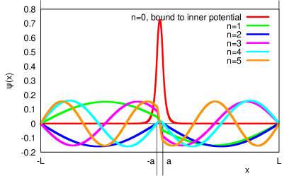
Figure 1: The first six wave functions for the double potential well. Here $2a=1.2$ fm and $L=100a$.

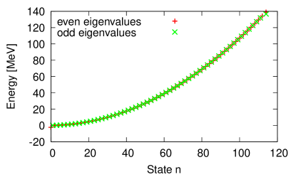
Figure 2: Energy eigenvalues for deuteron with binding energy of $-2.3$ MeV.

From the boundary conditions the following solutions for symmetric and antisymmetric wave emerge,

$$\psi_{1,<}^{s}(x) =A\left[\text{e}^{k_{1}^{s}x}-\text{e}^{-k_{1}^{s}(2L+x)}\right]$$ (6)

$$\psi_{2,<}^{s}(x) =A\frac{\left[\text{e}^{-k_{1}^{s}a}-\text{e}^{k_{1}^{s}(a-2L)}\right]}{\cos(k_{2}^{s}a)}\cos(k_{2}^{s}x)$$

$$\psi_{3,<}^{s}(x) =A\left[\text{e}^{-k_{1}^{s}x}-\text{e}^{k_{1}^{s}(x-2L)}\right]$$

$$\psi_{1,<}^{a}(x) =A\left[\text{e}^{k_{1}^{a}x}-\text{e}^{-k_{1}^{a}(2L+x)}\right]$$

$$\psi_{2,<}^{a}(x) =A\frac{\left[\text{e}^{-k_{1}^{a}a}-\text{e}^{k_{1}^{a}(a-2L)}\right]}{\sin(k_{2}^{a}a)}\sin(k_{2}^{a}x)$$

$$\psi_{3,<}^{a}(x) =-A\left[\text{e}^{-k_{1}^{a}x}-\text{e}^{k_{1}^{a}(x-2L)}\right]$$

for $E<0$ and

$$\psi_{1,>}^{s}(x) =A^{\prime}\frac{\sin(k_{1,n}(x+L))}{\sin(k_{1,n}L)}$$ (7)

$$\psi_{2,>}^{s}(x) =A^{\prime}\frac{\sin(k_{1,n}(L-a))}{\sin(k_{1,n}L)\cos(k_{2,n}a)}\cos(k_{2,n}x)$$

$$\psi_{3,>}^{s}(x) =A^{\prime}\frac{\sin(k_{1,n}(L-x))}{\sin(k_{1,n}L)}$$

$$\psi_{1,>}^{a}(x) =A^{\prime}\frac{\sin(k_{1,n}(x+L))}{\sin(k_{1,n}L)}$$

$$\psi_{2,>}^{a}(x) =A^{\prime}\frac{\sin(k_{1,n}(L-a))}{\sin(k_{1,n}L)\sin(k_{2,n}a)}\sin(k_{2,n}x)$$

$$\psi_{3,>}^{a}(x) =A^{\prime}\frac{\sin(k_{1,n}(L-x))}{\sin(k_{1,n}L)}$$

for $E>0$, where $A$ and $A^{\prime}$ are determined numerically to satisfy normalization, cf. fig. 1, and $s$ and $a$ denote parity even and odd real valued solutions, respectively. Finally, from the continuity condition

$$\left.\frac{\text{d}\psi_{1}(x)}{\text{d}x}\right|_{-a}=\left.\frac{\text{d}\psi_{2}(x)}{\text{d}x}\right|_{-a}$$

the equations for the energy eigenvalues

$$\tan(k_{2,n}^{s}a)=\frac{k_{1,n}^{s}}{k_{2,n}^{s}}\frac{1+\text{e}^{2k_{1,n}^{s}(a-L)}}{1-\text{e}^{2k_{1,n}^{s}(a-L)}}$$ (8)

for the symmetric and

$$\cot(k_{2,n}^{a}a)=-\frac{k_{1,n}^{a}}{k_{2,n}^{a}}\frac{1+\text{e}^{2k_{1,n}^{a}(a-L)}}{1-\text{e}^{2k_{1,n}^{a}(a-L)}}$$ (9)

for the antisymmetric wave functions follow, which are solved numerically. In fig. 2 the energy eigenvalues for the first 110 eigenstates are shown, using “deuteron parameters”, $2a=1.2$ fm, $E_{\text{bind}}=-2.3$ MeV Povh et al. (2014), resulting from choosing the potential $V_{0}=-18$ MeV and $L=100$ fm. In the calculation, $m$ is chosen to be the reduced mass $m_{\text{p}}/2$ Povh et al. (2014). Comparing eq. 8 and eq. 9 with eq. 5, one realizes from fig. 2, that $E_{n}\sim n^{2}$ for large $n$. For small $n$ the growth is not exactly quadratic, due to the exponential parts of eq. 8 and eq. 9. For the chosen parameters there is only one “bound state” with $E<0$.

For the following numerical calculations the energy eigenbasis up to the $110^{\text{th}}$ state will be truncated, which corresponds to an energy cut-off of about $140$ MeV. As will be discussed in the next section, the eigenbasis will serve as a restricted Hilbert space.

III Time dependent wave function

In the following we employ the energy eigenfunctions of $\hat{H}_{0}$ to solve the time-dependent problem,

$$\begin{split}i\hbar\partial_{t}\psi(x,t)&=\hat{H}\psi(x,t)\\ &=\left[-\frac{\hbar^{2}}{2m}\partial_{x}^{2}+V_{0}(x)+V(x,t)\right]\psi(x,t),\end{split}$$ (10)

where $V(x,t)$ represents a time-dependent “external potential”. Expanding the state in terms of the $\hat{H}_{0}-$eigenstates $\ket{\psi_{n}}$,

$$\ket{\psi}=\sum_{n}c_{n}(t)\ket{\psi_{n}},$$ (11)

it follows for the time-dependent Schrödinger equation

$$\begin{split}\mathrm{i}\hbar\frac{\mathrm{d}}{\mathrm{d}t}\ket{\psi}&=\mathrm{i}\hbar\sum_{n}\dot{c}_{n}(t)\ket{\psi_{n}}\\ &=\hat{H}\ket{\psi}=\sum_{n}c_{n}(t)\left[E_{n}+\hat{V}\right]\ket{\psi_{n}},\end{split}$$ (12)

where $E_{n}$ are the eigenvalues of $\hat{H}_{0}$. Multiplying with $\bra{\psi_{j}}$ leads to

$$\mathrm{i}\hbar\dot{c}_{j}(t)=E_{j}c_{j}(t)+\sum_{n}V_{jn}(t)c_{n}(t)$$ (13)

with the matrix elements

$$V_{jn}(t)=\left\langle{\psi_{j}}\left|\vphantom{\psi_{j}\psi_{n}}{\hat{V}}\right|{\psi_{n}}\right\rangle.$$ (14)

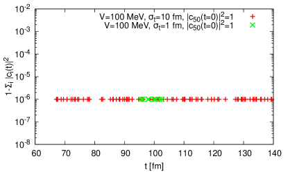
Figure 3: $1-\sum_{n}|c_{n}(t)|^{2}$ for a single pulse at $t=100$ fm with $\sigma_{x}=1.2$ fm.

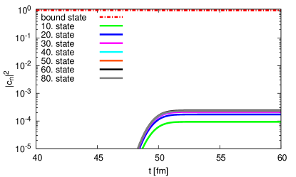
Figure 4: $|c_{n}(t)|^{2}$ with a time dependent potential. The bound state is originally populated, $|c_{0}(t=0)|=1$ and $|c_{n\neq 0}(t=0)|=0$, $\sigma_{t}=1$ fm and $\sigma_{x}=0.2a=0.12$ fm, furthermore $t_{0}=50$ fm and $V=100$ MeV.

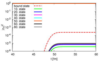
Figure 5: $|c_{n}(t)|^{2}$ with a time dependent potential. Here $|c_{50}(t=0)|=1$ and $|c_{n\neq 50}(t=0)|=0$, $\sigma_{t}=1$ fm and $\sigma_{x}=0.2a=0.12$ fm, $t_{0}=50$ fm and $V=100$ MeV.

This set of first-order differential equations can be simplified by the ansatz

$$c_{j}(t)=\tilde{c}_{j}(t)\mathrm{e}^{-\text{i}E_{j}t/\hbar},$$ (15)

which leads to

$$\text{i}\hbar\dot{\tilde{c}}_{j}(t)=\sum_{n}V_{jn}(t)\exp\left(\text{i}\omega_{jn}t\right)\tilde{c}_{n}(t),$$ (16)

where we have defined the transition frequencies $\omega_{jn}=(E_{j}-E_{n})/\hbar$.

For the numerical solution of the infinite coupled set of differential equations eq. 16 we truncate the expansion by using the first 110 eigenstates only and use a fourth-order Runge-Kutta solver. Then $\sum_{n}|c_{n}(t)|^{2}=1$ for all $t$. To evaluate the accuracy of the numerical results, we show this conservation of the normalization of the state, which should hold exactly since in the truncated Hilbert space the matrix $V_{nm}=\braket{n}{\hat{V}}{m}$ is Hermitian. As illustrated in fig. 3 (the parameters are detailed in section IV and VII) the norm of the numerically calculated state at $t=100\;\,{\rm fm}$ deviates from 1 only by about $10^{-6}$, and proves the high accuracy of the numerical integration of the coupled set of linear differential equations (16).

IV Time dependent Potential and Dynamics of States

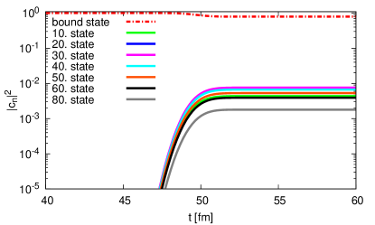
Figure 6: $|c_{n}(t)|^{2}$ with a time dependent potential. The bound state is originally populated, $|c_{0}(t=0)|=1$ and $|c_{n\neq 0}(t=0)|=0$, $\sigma_{t}=1$ fm and $\sigma_{x}=1.2$ fm, $t_{0}=50$ fm and $V=100$MeV.

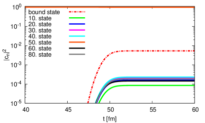
Figure 7: $|c_{n}(t)|^{2}$ with a time dependent potential. Here $|c_{50}(t=0)|=1$ and $|c_{n\neq 50}(t=0)|=0$, $\sigma_{t}=1$ fm and $\sigma_{x}=1.2$ fm, $t_{0}=50$ fm and $V=100$ MeV.

As already discussed, the “deuteron parameters” for the one-dimensional square well potential in a box are given by a potential depth of $V_{0}=-18$ MeV, a diameter of $2a=1.2$ fm and a binding energy of $-2.3$ MeV. This value of $V_{0}$ deviates from the value given in Povh et al. (2014), as there the three-dimensional case of a spherical symmetric cavity is considered with $V_{0}=-57$ MeV. However, for simplification we discuss the one-dimensional case here. In the following calculations we take a time dependent Gaussian potential, which reads

$$\begin{split}V(x,t)=&V\exp\left[-\frac{(x-x_{0})^{2}}{2\sigma_{x}^{2}}\right]\left[\exp\left(-b(t-t_{0})^{2}\right)\right.\\ &\left.+\exp\left(-b(t-t_{1})^{2}\right)+\cdots\right.\\ &\left.+\exp\left(-b(t-t_{N})^{2}\right)\right],\end{split}$$ (17)

with $b=\frac{1}{2\sigma_{t}^{2}}$, where $t_{0},t_{1},...,t_{N}$ are the $N$-times, when “potential pulses” interact with the system. We take $x_{0}=0$ as the potential should disturb the system where the bound/ground state is well localized.

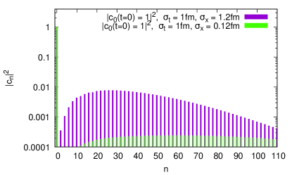
Figure 8: $|c_{n}(t\gg t_{0})|^{2}$ after the impact of the time dependent potential. Here $|c_{0}(t=0)|=1$ and $|c_{n\neq 0}(t=0)|=0$ for different space width, cf. fig. 4 and fig. 6. $V=100$ MeV.

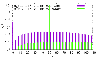
Figure 9: $|c_{n}(t\gg t_{0})|^{2}$ after the impact of the time dependent potential. Here $|c_{50}(t=0)|=1$ and $|c_{n\neq 50}(t=0)|=0$ for different space width, cf. fig. 5 and fig. 7. $V=100$ MeV.

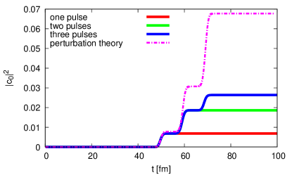
Figure 10: $|c_{0}(t)|^{2}$. Bound state formation after three pulses, with $|c_{20}(t=0)|^{2}=1$, $\sigma_{t}=1$ fm, $\sigma_{x}=1.2$ fm, $V=100$ MeV. The dashed line represents the same calculation in first order perturbation theory (cf. section VI).

At first the situation is given by the interaction of one single pulse. The parameters, which were chosen here are either $\sigma_{x}=2a=1.2$ fm or $\sigma_{x}=0.2a=0.12$ fm to study the impact of the spatial width of the potential and apply various time durations $\sigma_{t}$. In fig. 4 one can see, that if the bound state, corresponding to the binding energy of a deuteron, $-2.3$ MeV, is originally populated, $|c_{0}(t=0)|^{2}=1$, and the system interacts with a time dependent potential at some time, here for $t_{0}=50$ fm and $\sigma_{t}=1$ fm, the excited states are populated right at the arrival of the pulse, and the originally prepared bound state decreases correspondingly. For $\sigma_{x}=0.2a$ the bound state is depopulated by about $4\%$, and the system has gained a small energy increase due to the interaction, cf. fig. 4. On the other hand, if $\sigma_{x}$ is larger, here $2a$, then the originally populated bound state is depopulated by about $30\%$, also the mean population of the other states grows by orders of magnitude, cf. fig. 6.

One can observe this behavior also if the 50th state is populated originally and then decays after the impact of the potential, cf. fig. 5 and fig. 7. In both cases, $\sigma_{x}=0.2a$ and $\sigma_{x}=2a$, $|c_{50}(t\gg t_{0})|^{2}$ ($E_{50}\approx 26$ MeV, cf. fig. 2) decreases slightly, while the bound state reacts strongly and also almost instantaneously on the time scale $\sigma_{t}$. Due to the large energy gap the bound state populates by more than an order of magnitude stronger than the other excited states. In fig. 8 one can see the distribution of populated states if the bound state is originally prepared and $\sigma_{x}$ is varied between $\sigma_{x}=0.2a$ and $\sigma_{x}=2a$. All the other parameters in eq. 17 are kept fixed at $\sigma_{t}=1\,\text{fm}$ and $V=100\,\text{MeV}$. One finds a small decrease of the bound state, $n=0$, and an increase of all the other states after the impact of the potential.

Figure 11: Stochastic potential with 1000 equidistant timesteps and Gaussian distributed potential strength.

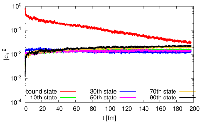
Figure 12: Averaged $|c_{n}(t)|^{2}$ of a Gaussian distributed stochastic potential with 2000 pulses with initial conditions $|c_{0}(t=0)|^{2}=1$ and $|c_{n\neq 0}(t=0)|^{2}=0$. Here $\sigma_{x}=1.2$ fm and the potential given in eq. 18.

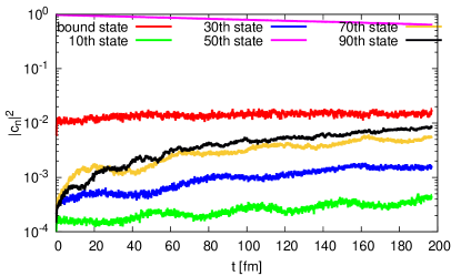
Figure 13: Averaged $|c_{n}(t)|^{2}$ of a Gaussian distributed stochastic potential with 2000 pulses with initial conditions $|c_{50}(t=0)|^{2}=1$ and $|c_{n\neq 50}(t=0)|^{2}=0$. Here $\sigma_{x}=1.2$ fm and the potential given in eq. 18.

It is important to mention, that increasing the spatial width of the pulse does not lead to a linear increase in the state formation, but also lead to a different shape of the distribution in the states. One can see in fig. 8, that a larger $\sigma_{x}$ narrows the distribution, such, that they are Breit-Wigner-like distributed around the 25th state, which corresponds to an energy of $\sim 3\,\text{MeV}$, cf. fig. 2. If the 50th state is populated originally, then after the impact of the pulse, $|c_{50}(t)|^{2}$ decreases slightly, as already mentioned. The bound state forms dominantly, compared to the other states. The most important difference is, that the states populate in a broad distribution, whose broadness is not dominantly determined by $\sigma_{x}$, cf. fig. 9. Of course a wider pulse leads to a stronger population of the states.

We will continue the discussion of the results of fig. 8 and fig. 9 in section VII, where the impact of the interaction time $\sigma_{t}$ on the distribution of states will be investigated in more depth, in order to understand the interplay between the energy distribution and the pulse duration in terms of Heisenberg’s uncertainty relation of energy and time. The impact of a longer and a shorter pulse and taking $\sigma_{x}=1.2$ fm refers to a particle, which interacts with a deuteron, having a similar size in the interaction channel.

Following eq. 17, one also can easily increase $N$, the number of pulses, for example $N=2$ and $N=3$, cf. fig. 10. One can see, that after each pulse, the bound state will be increasingly populated. The other states will populate similarly in time (with other amplitudes) and the 20th state will depopulate accordingly. In addition, the results (purple dashed line) of first order perturbation theory for this particular situation is also depicted and will be discussed briefly in section VI.

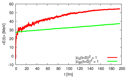
Figure 14: Mean energy, cf. eq. 19, of a Gaussian distributed stochastic potential with 2000 pulses.

V Randomized potential pulses

To briefly study the behavior of a system, that interacts all the time with a stochastic potential, such as a random noise, we increase the number of pulses $N$ to an order of $\mathcal{O}(2000)$, where $t_{i+1}=t_{i}+\Delta t$, with a Gaussian distributed amplitude $V_{\xi}$ with $\braket{V_{\xi}}=0$ and $\sigma_{V}=50$ MeV,

$$\begin{split}V(x,t)=&\sum_{j=1}^{N}V_{\xi}\exp\left(-\frac{x^{2}}{2\sigma_{x}^{2}}\right)\\ &\left[\Theta(t-jn\Delta t)-\Theta(t-j(n+1)\Delta t)\right].\end{split}$$ (18)

Furthermore, the parameters are taken as $\Delta t=0.02\,\,{\rm fm}$ and $\sigma_{x}=1.2\,\,{\rm fm}$, and the real value $n$ is set to be $n=5$, which means, that numerically every 5th time step a random pulse occurs. This corresponds to the interaction of the nuclei with random “bath particles”, which leads to the formation and dissociation of bound states or other quantum states as described above. Generating this statistical potential leads to the potential profile illustrated in fig. 11.

In the following we take ensemble averages of the time evolution over these random potentials. Figs. 12 and 13 show the evolution of states under the influence of a potential with 2000 pulses, employing two different initial conditions: (a) the bound state originally populated and (b) the 50th state originally populated; the results are averaged over 200 Monte-Carlo realizations of the random process, $V(x,t)$. It turns out that the initially prepared state is depopulated continuously and the other states get correspondingly occupied. As illustrated in fig. 13 the bound state forms on a very small timescale, i.e., rather instantly. The bound state reacts fastest to the impact of the pulses, cf. fig. 13, red line, since the state of smallest and distinct energy is preferably populated.

As illustrated in fig. 14, the mean energy of the system,

$$\braket{E(t)}=\frac{\sum_{n}E_{n}|c_{n}(t)|^{2}}{\sum_{n}|c_{n}(t)|^{2}}=\sum_{n}E_{n}|c_{n}(t)|^{2},$$ (19)

starts at $t=0$ with the $n$-th energy eigenvalue of the initialized state and then continuously increases due to the time-dependent external potential. This behavior as found stands in contrast to a potential equilibration of the system, that should occur for $t\rightarrow\infty$, if we consider the system as coupled to a potential heat bath of random particles, or interactions. In principle energy dissipation has to be incorporated as an additional ingredient for the propagation of the particle in the system, in analogy to the classical Langevin equation,

$$\dot{p}=-\gamma p+f(t).$$ (20)

Dissipation and fluctuation are intimately related. The further development of a consistent quantum-theoretical description for the formation of bound states in open quantum systems is an intriguing question, and is relevant in particular for the microscopic understanding of the production of light nuclei Danielewicz and Bertsch (1991) or heavy quarkonia states in relativistic heavy ion collisions Katz and Gossiaux (2016); Blaizot and Escobedo (2018); Rothkopf (2020). Powerful non-equilibrium quantum formalisms to evaluate the equilibration of an open quantum system, including dissipation, are given by the Kadanoff-Baym equations Danielewicz (1984); Greiner and Leupold (1998) or by the Caldeira-Leggett master equation Caldeira and Leggett (1983), both of which describe the time evolution of the system in terms of (reduced) density matrices or Green’s functions.

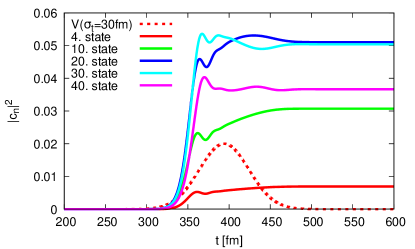
Figure 15: Non-perturbative behavior of the system, reacting on a long pulse, here $\sigma_{t}=30$ fm, $\sigma_{x}=1.2$ fm and $V=100$MeV, centred at $t_{0}=400$ fm and $|c_{0}(t=0)|^{2}=1$. Green dashed line indicates the shape of the pulse.

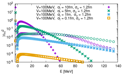
Figure 16: First order perturbation theory for different $V$, $\sigma_{t}$ and $\sigma_{x}$. The circles represent the exact numerical solution corresponding to the same color in perturbation theory.

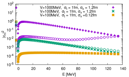
Figure 17: First order perturbation theory for different $V$ and $\sigma_{x}$. The circles represent the exact numerical solution corresponding to the same color in perturbation theory.

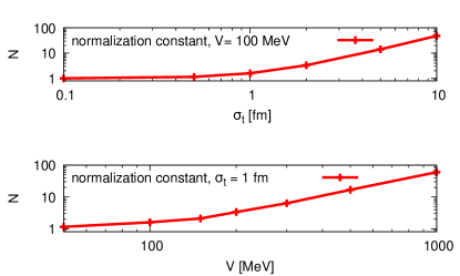
Figure 18: $N$ in first order perturbation theory for different $V$, $\sigma_{t}$ at $\sigma_{x}=1.2$ fm.

VI Perturbation theory

In this Sec. we also want to study the applicability of perturbation theory, i.e., we validate Fermi’s golden rule, i.e., first order perturbation theory, which allows the description of the transition amplitude from an initial state $i$ to a final state $f$ via $|c_{n}(t)|^{2}$,

$$c_{f}^{(1)}(t) =\delta_{fi}-\frac{\text{i}}{\hbar}\int_{t_{0}}^{t}\text{d}t^{\prime}V_{fi}(t^{\prime}),$$ (21)

where $V_{fi}(t^{\prime})=V(t^{\prime})\exp(-\text{i}\omega_{fi}t^{\prime})$ Landau and Lifshitz (1981). To set the stage, in fig. 15 the highly non-perturbative behavior of a long pulse is clearly demonstrated.

Intuitively and regarding eq. 21 first order perturbation theory should be valid if $\frac{1}{\hbar^{2}}|\int\text{d}tV_{fi}|^{2}\ll 1$. Furthermore, (cf. Langhoff et al. (1972)) first order perturbation theory is not normalized. Therefore it is a reasonable method to evaluate the applicability of perturbation theory by considering the “normalization constant”, $N=1/\sqrt{\sum_{n}|c_{\text{n, pert}}|^{2}}$. In the case of fig. 15, $N\approx 74$, which is much larger than one and proves, that here perturbation theory is not applicable.

To study the validity of perturbation theory for different model parameters, in fig. 16 $|c_{n}(t\gg t_{0})|^{2}$ different pulse lengths $\sigma_{t}$ are shown. In fig. 17 the potential strengths are set to either $V=100$ MeV or $V=1000$ MeV and also the widths are either $\sigma_{x}=0.12\,\,{\rm fm}$ or $\sigma_{x}=1.2\;\,{\rm fm}$, while $\sigma_{t}$ is set constantly at 1 fm and first-order perturbation theory is compared to the exact numerical results in the case of one pulse at $t_{0}=50\,\,{\rm fm}$. The circles of the same color refer to the same parameters as the perturbative ones but represent the exact results solving the time-dependent Schrödinger equation. In fig. 18 the normalization constant, $N$, is shown for different values of $\sigma_{t}$ while keeping $V=100\,\,{\rm MeV}$ constant, and for different values of $V$ while keeping $\sigma_{t}=1\,\,{\rm fm}$ constant.

As shown in fig. 16, for $\sigma_{t}=1$ fm and $\sigma_{t}=0.1$ fm for a potential of $V=100$ MeV and $\sigma_{x}=1.2$ fm perturbation theory and the numerical results are still applicable and thus in reasonable agreement. If one increases $\sigma_{t}$, such that $\sigma_{t}=5$ fm or $\sigma_{t}=10$ fm the perturbative results deviate from the numerical ones, not only by a factor but also in the shape of the distribution. For $V=1000$ MeV instead, cf. fig. 17, all perturbative results lie about two orders of magnitude above the exact numerical results.

As expected, the perturbative results for $V=1000$ MeV deviate from the ones for $V=100$ MeV by a factor of 100, cf. eq. 21. Furthermore the shape of the distribution changes, because for the numerical results the $|c_{n}|^{2}$ increase for higher energies. This is due to the fact, that $V=1000$ MeV exceeds the highest energy of $\approx 140\;\,{\rm MeV}$ taken into account in the truncated Hilbert space. On the other hand, the norm is conserved due to the unitarity of the time evolution in the truncated Hilbert space, $\sum_{n}|c_{n}|^{2}=1$, which leads to a higher occupation of the higher states. This of cause does not affect the calculation in perturbation theory.

For $V=100$ MeV, $\sigma_{t}=1\,\,{\rm fm}$ but $\sigma_{x}=0.12\,\,{\rm fm}$ perturbation theory agrees satisfactorily with the exact numerical results. Considering a typical pulse duration of an interacting particle having a similar size as a deuteron ($\sigma_{x}=1.2\;\,{\rm fm}$), of about $\sigma_{t}=1\;\,{\rm fm}$ and $50$-$150\;\,{\rm MeV}$, thus agrees reasonably well with the exact calculation. As depicted in fig. 18, increasing the potential, $V$, and/or the duration of the pulses, $\sigma_{t}$, leads to an increase of $N$ and therefore the failure of perturbation theory. E.g., for $\sigma_{t}\approx 5$ fm $N$ is already about $10$ times larger than for $\sigma_{t}=1$ fm. For larger potentials, the normalization diverges more or less quadratically. In a range of $\sigma_{t}=1$ fm and $V=100$ MeV, $N$ is about 1, indicating that perturbation theory is a good approximation for this parameter setting.

Therefore one can conclude, that perturbation theory is applicable for weak potentials in comparison to the considered energy range of the system and for short interaction times of about 1 fm. Furthermore, one can see, that an increase of either parameter leads to an increase of the error of the perturbative results, which is due to the fact, that $\frac{1}{\hbar^{2}}|\int\text{d}tV_{fi}|^{2}\ll 1$ should hold as an applicability criterion for first order perturbation theory. Correspondingly, if one increases the number of pulses, cf. fig. 10, where the number of three pulses has been considered, the perturbative calculation provides significantly different results than the numerical calculation due to the fact, that in the integral of eq. 21 the contributions from the subsequent pulses just add up, while in the full calculation all states get populated already after the first pulse considerably, which is not taken into account in eq. 21. In order to improve the applicability of perturbation theory, one has to modify the ansatz to obtain correct rate equations in form of a (norm-conserving) master equation, which takes into account gain and loss of the states after every single pulse. This is the legitimation of a (quantum) kinetic master equation or Boltzmann-type equation.

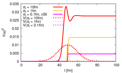
Figure 19: Formation of states during a pulse with $\sigma_{t}=10$ fm, $\sigma_{t}=1$ fm and $\sigma_{t}=0.01$ fm (here $|c_{30}(t,\sigma_{t}=0.1\text{ fm})|^{2}$ multiplied by a factor of 50, for visualization), $\sigma_{x}=1.2$fm and $V=100$MeV, $|c_{0}(t=0)|^{2}=1$.

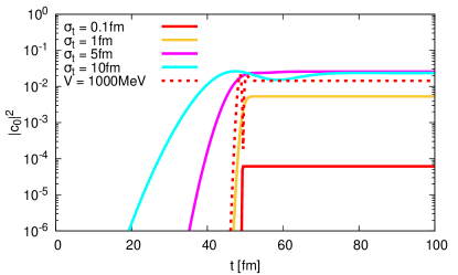
Figure 20: Bound state formation of $|c_{50}(t=0)|^{2}=1$ for different time length (solid lines) at $V=100$ MeV and a comparison of a strong potential of $1000$ MeV with $\sigma_{t}=1$ fm (dashed line), one pulse.

VII Heisenberg’s energy-time uncertainty relation

A seemingly straight-forward expectation is that the formation of states, especially bound states, underlies the Heisenberg’s uncertainty relation in energy and time. A disturbance of the system caused by an interacting particle, e.g. a collision or here the time-dependent potential, leads to a reaction of the system which then rearranges its energy distribution over the available states. One possible idea is, that this rearrangement underlies the uncertainty relation in energy and time such, that the system needs some time $\Delta t$, which is the difference between the potential impact and the reaction of the system, which then is dependent on the energy,

$$\tau_{\text{f}}\sim\frac{\hbar}{E_{\text{D}}}\quad\text{or}\quad\tau_{\text{f}}\sim\frac{\hbar}{E_{\text{B}}},$$ (22)

where $\tau_{\text{f}}$ is then the “formation time” of for example a deuteron, and $E_{\text{D}}$ the energy difference of a certain state before and after the interaction or even simply the binding energy, $E_{\text{B}}$.

In contradiction to this possible straight-forward idea, as demonstrated in fig. 19 and fig. 20, the states form immediately, independently of the pulse duration (cf. also fig. 4-fig. 7). Especially in fig. 19 we decrease the pulse duration to only $0.1$ fm (pink line) and find, that still the state reacts immediately to the pulse.

Therefore, as illustrated by these results, Heisenberg’s uncertainty relation in energy and time should be understood in a different way. It is more suitable to talk about the population time instead of the formation time, because we want to point out, that the formation time is equivalent to the interaction time of the potential, and therefore the term is misleading. This picture is also in good agreement with the interpretation of the energy-time uncertainty relation given in Landau and Lifshitz (1981) and Messiah (1999), which is motivated by considering the transition probability from the energy eigenstate $\psi_{i}$ to the energy eigenstate $\psi_{f}$ of the unperturbed system, due to the external potential. In first-order perturbation theory the transition amplitude is given by eq. 21, which reads, rewritten for our present case of a potential (17) representing only one pulse

$$\begin{split}c_{f}(t)=-\text{i}\frac{V_{fi}}{\hbar}\int_{-\infty}^{t}\text{d}t^{\prime}&\exp\left(-\frac{(t^{\prime}-t_{0})^{2}}{2\sigma_{t}^{2}}\right)\\ &\exp(\text{i}\omega_{fi}t^{\prime})\end{split}$$ (23)

where $\omega_{fi}=\Delta E/\hbar$ and

$$V_{fi}=\int_{\mathbb{R}}\mathrm{d}xV\psi_{f}^{*}(x)\exp\left[-\frac{(x-x_{0})^{2}}{2\sigma_{x}^{2}}\right]\psi_{i}(x).$$ (24)

In the limit $t\rightarrow\infty$ the probability for a transition of the particle from an energy eigenstate $\psi_{i}$ through the perturbation of duration $\sigma_{t}$, adiabatically switched on and off via the Gaussian time dependence, reads

$$\begin{split}S_{fi}&=\lim_{t\rightarrow\infty}c_{f}(t)\\ &=-\mathrm{i}\sqrt{2\pi}\frac{V_{fi}}{\hbar}\sigma_{t}\exp\left[-\frac{1}{2}\sigma_{t}^{2}\omega_{fi}^{2}\right],\end{split}$$ (25)

and therefore the transition probability is

$$|S_{fi}|^{2}=2\pi\frac{|V_{fi}|^{2}\sigma_{t}^{2}}{\hbar^{2}}\exp\left[-\sigma_{t}^{2}\omega_{fi}^{2}\right].$$ (26)

This implies that the smaller $\Delta t\simeq\sigma_{t}$, the broader is the distribution of the observed changes of energy.

In App. B we give a more general, non-perturbative interpretation of the time-energy uncertainty relation, related to the accuracy of “time and energy measurements”. This is in accordance with Landau and Lifshitz (1981), where it is pointed out, that the uncertainty relation in energy and time can not be interpreted as a uncertainty of measurement in energy at a certain time, as the uncertainty relation in position and momentum, but is the difference of energies, that are measured at two different times.

Figure 19 illustrates, that the system reacts immediately to the pulse. The dashed lines indicate the pulse, and a randomly picked state reacts immediately to the potential, independently of the pulse duration. If one decreases $\sigma_{t}$ even more ($\sigma_{t}=0.1$ fm), then the states populate still immediately with the appearance of the potential. This is valid also for a system, where $n=50$ is originally prepared and the bound state is populated due to the perturbation, as can be seen in fig. 20. Also the occupation of the states stays constant immediately after the perturbation is switched off, cf. fig. 19 and fig. 20. As shown in fig. 19, if one applies a very short pulse, dashed pink line (potential) and pink line (state), where the pulse is $\sigma_{t}=0.1\;\,{\rm fm}$, the states get populated immediately, as suggested above. In fig. 3 we show the conservation of the norm during the time evolution for $\sigma_{t}=1$ fm and $\sigma_{t}=10$ fm, which demonstrates the high numerical accuracy of the calculation. In fig. 20 one can also see, that a stronger potential, here $1000$ MeV, does not automatically lead to a stronger increase in the states, but leads to oscillations during the pulse, which shows again, that first-order perturbation theory is not applicable in this case.

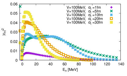
Figure 21: Distribution of $|c_{n}(t_{\text{final}})|^{2}$, comparing different $\sigma_{t}$ and $V$. $\sigma_{x}=1.2$ fm, with initial condition $|c_{0}(t=0)|^{2}=1$.

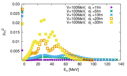
Figure 22: Distribution of $|c_{n}(t_{\text{final}})|^{2}$, comparing different $\sigma_{t}$ and $V$. $\sigma_{x}=1.2$ fm, with initial condition $|c_{50}(t=0)|^{2}=1$.

Heisenberg’s energy uncertainty relation,

$$\Delta E\Delta t\geq\frac{\hbar}{2},$$ (27)

should be interpreted as

$$\Delta E\cdot\sigma_{t}\geq\frac{\hbar}{2},$$ (28)

where $\Delta E$ is the standard deviation of the energy of the final distribution of states, as illustrated in fig. 21 and fig. 22, and $\sigma_{t}$ is the standard deviation of the pulse length. Let us therefore consider the yellow dots, which represent a pulse of length $\sigma_{t}=30\,\,{\rm fm}$. The expectation value for the energy lies here at $\approx 9$ MeV and the width of the distribution is $\approx 12$ MeV. Therefore we obtain an energy spread of $\Delta E\approx 24$ MeV. If $\sigma_{t}=30\,\,{\rm fm}$, we obtain

$$\Delta E\sigma_{t}\geq\frac{\hbar}{2}\leftrightarrow 24\text{ MeV}\cdot\frac{30\text{ fm}}{197\text{ MeV fm}}\approx 3.65>\frac{1}{2},$$ (29)

which shows, that the interaction time could still be enlarged, to obtain a narrower distribution. For smaller $\sigma_{t}$, for example $\sigma_{t}=1,5,10$ fm, more states are excited and the energy distribution gets broader. This can also be seen in the strength of the excitation, which means the amplitude in $|c_{n}(t\gg t_{0})|^{2}$. The longer the interaction time of the potential with the system, the more a certain state is populated and the more the distribution peaks at a certain point. If one increases $\sigma_{t}$, then the distribution shifts to the left. We want to mention here, that those states, that were originally prepared in fig. 21 and fig. 22 are above the range of the axis of abscissas in both figures. This is due to the fact, that for small $\sigma_{t}$ the destruction of the initial state is not significant. The width of each peak in the distribution is never less than the limiting value of $\frac{\hbar}{\sigma_{t}}$, in accordance with Heisenberg’s uncertainty relation in energy and time. Therefore we can conclude, that the Heisenberg’s uncertainty relation in energy and time describes, which energy states are occupied after a perturbation, but not how fast. As illustrated in fig. 21, for $\sigma_{t}=10$ fm, and especially in fig. 22 there are two or three peaks at certain energies in the distribution, which correspond to further excitations of the systems of higher orders, similar to the harmonics of a string, corresponding to the energy differences $\hbar\omega_{mn}$.

VIII Conclusions and Outlook

To address the question of bound-state formation and dissociation under the influence of time-dependent perturbations we have investigated a simple one-dimensional model of a particle in a square-well potential, which has been adjusted such that only one bound state exists (analogous to the case of the deuteron). After solving the energy eigenproblem we have solved numerically the time evolution of the system under the influence of Gaussian time-dependent pulses. We have demonstrated, that disturbing the system with such a pulse leads to the excitement of higher energy states and a de-excitement of the bound state, if the bound state is originally fully populated. On the other hand a before unoccupied bound state can be formed due to the interaction with the pulse. Due to the large energy gap, the bound state reacts fastest and evolves in accordance with the pulse. After the interaction with the potential the state remains constant. Increasing the number of pulses and applying stochastic pulses to simulate a thermal bath interacting with the system leads to a decrease of the originally populated state and an increase of all other states.

We have investigated the regime in which first-order perturbation theory is applicable and therefore in a good agreement with the numerical results. First-order perturbation theory is applicable for short interaction times, $\sim 1\,\,{\rm fm}$ and energies $\sim 50\,\,{\rm MeV}$ to $\sim 150\,\,{\rm MeV}$. Furthermore, the spacial width of the potential should be small. We have also shown, that first-order perturbation theory should be modified in order to obtain a (norm-conserving) master equation, if one increases the number of pulses.

We have demonstrated, that the system adjusts its states simultaneously to the potential, independent of the duration of the pulse. We have shown, that Heisenberg’s uncertainty relation for energy and time is fulfilled in standard deviations of the energy distributions of the various quantum states and the standard deviation of the duration of the time-dependent perturbation. Therefore we have seen, that strong and long pulses interact with the system such, that the potential leads to certain excitations of energies, which are characterized by the energy differences, $\hbar\omega_{mn}$. The width of the distribution is related to Heisenberg’s uncertainty relation in energy and time and does not fall below the limit of $\Delta E\geq\frac{1}{2\sigma_{t}}$. On the other hand, short pulses lead to a weak population of all energy states of the system. Nevertheless, there is no time delay in the excitation or de-excitation of a state due to the impact of an interacting potential, but the states rearrange immediately after the impact of the time-dependent potential. There is no upper limit of $\braket{E(t)}$, because the time dependent potential provides the system with additional energy all the time.

Since the system is not damped due to a quantum mechanical (dissipative) Langevin equation the aim of further studies is to develop a non-equilibrium quantum formalism and evaluate the equilibration of an open quantum system including distinct bound states, in which our model serves as a system particle, and dissipation and fluctuation of energy are introduced by the interaction with a thermal environment. This will be achieved by employing the influence-functional formalism and the Caldeira-Leggett master equation in a Lindblad approach Rais and contemporaneously by the use of the Kadanoff-Baym equations Neidig , to microscopically understand the production of light nuclei, i.e., the deuteron or heavy quarkonia states. As a further improvement, the model will be extended to three dimensions.

Appendix

Appendix A Conservation of the norm $\sum_{n}|c_{n}(t)|^{2}$

Let $\psi(t,x)$ be the wave function and taking the time derivative of the norm,

$$\begin{split}&\frac{\text{d}}{\text{d}t}\int_{-L}^{L}\text{d}x|\psi(x,t)|^{2}=\int_{-L}^{L}\text{d}x\frac{\text{d}}{\text{d}t}|\psi(x,t)|^{2}\\ &=\int_{-L}^{L}\text{d}x\frac{\partial}{\partial t}(\psi^{*}(x,t)\psi(x,t))\\ &=\int_{-L}^{L}\text{d}x\left[\psi^{*}(x,t)\frac{\partial\psi(x,t)}{\partial t}+\frac{\partial\psi^{*}(x,t)}{\partial t}\psi(x,t)\right].\end{split}$$ (30)

Using the Schrödinger equation,

$$\frac{\partial\psi(x,t)}{\partial t}=\frac{\text{i}\hbar}{2m}\frac{\partial^{2}\psi(x,t)}{\partial x^{2}}-\frac{\text{i}}{\hbar}V(x,t)\psi(x,t)$$ (31)

and its complex conjugate

$$\frac{\partial\psi^{*}(x,t)}{\partial t}=-\frac{\text{i}\hbar}{2m}\frac{\partial^{2}\psi^{*}(x,t)}{\partial x^{2}}+\frac{\text{i}}{\hbar}V(x,t)\psi^{*}(x,t),$$ (32)

we obtain

$$\begin{split}&\frac{\partial}{\partial t}|\psi(x,t)|^{2}=\psi^{*}(x,t)\frac{\text{i}\hbar}{2m}\frac{\partial^{2}\psi^{*}(x,t)}{\partial x^{2}}\\ &-\frac{\text{i}}{\hbar}V(x,t)\psi(x,t)\psi^{*}(x,t)\\ &\qquad-\psi(x,t)\frac{\text{i}\hbar}{2m}\frac{\partial^{2}\psi^{*}(x,t)}{\partial x^{2}}\\ &+\frac{\text{i}}{\hbar}V(x,t)\psi(x,t)\psi^{*}(x,t)\\ &=\frac{\text{i}\hbar}{2m}\left(\psi^{*}(x,t)\frac{\partial^{2}\psi(x,t)}{\partial x^{2}}-\frac{\partial^{2}\psi^{*}(x,t)}{\partial x^{2}}\psi(x,t)\right)\\ &=\frac{\partial}{\partial x}\left[\frac{\text{i}\hbar}{2m}\left(\psi^{*}(x,t)\frac{\partial\psi(x,t)}{\partial x}-\frac{\partial\psi^{*}(x,t)}{\partial x}\psi(x,t)\right)\right].\end{split}$$

This leads, inserting into LABEL:Schroednorm to

$$\frac{\text{d}}{\text{d}t}\int_{-L}^{L}\text{d}x|\psi(x,t)|^{2}$$

$$=\frac{\text{i}\hbar}{2m}\left.\left(\psi^{*}(x,t)\frac{\partial\psi(x,t)}{\partial x}-\frac{\partial\psi^{*}(x,t)}{\partial x}\psi(x,t)\right)\right|_{-L}^{L}.$$

With the boundary condition $\psi(\pm L,t)=0$ it follows

$$\frac{\text{d}}{\text{d}t}\int_{-L}^{L}\text{d}x|\psi(x,t)|^{2}=0.$$

Expanding the wave function,

$$\psi(x,t)=\sum_{n=0}^{m}c_{n}(t)\psi_{n}(x),$$

also

$$\frac{\text{d}}{\text{d}t}\sum_{n=0}^{m}|c_{n}(t)|^{2}=0$$

holds. This is valid for any $m$, because the “truncated” matrix $H_{jk}=\braket{\psi_{j}}{\hat{H}}{\psi_{k}}$, with $j,k\in\left\{0,1,...,m\right\}$ is Hermitian.

Appendix B Interpretation of the energy-time uncertainty relation

In this Appendix we briefly discuss the meaning of the “energy-time uncertainty relation”, following Messiah (1999); Landau and Lifshitz (1981); Mandelstam and Tamm (1945). Particularly we want to emphasize that $\Delta t$ does not refer to a kind of “formation time” for bound states in a medium.

It is important to note that the energy-time uncertainty relation needs a special consideration concerning its interpretation since in quantum mechanics time cannot be treated as an observable. As has been argued by Pauli Pauli (1980), time cannot be interpreted as an observable in quantum theory since then it would be represented by a self-adjoint operator, $\hat{t}$, and since the Hamilton operator, which represents the energy of the system, by definition is the generator of the time evolution, it had to fulfill the commutation relation $[\hat{t},\hat{H}]=-\mathrm{i}\hbar$. Then the usual argument familiar from the analogous situation for position and momentum operators leads to entire $\mathbb{R}$ as the spectrum for $\hat{H}$. This would imply that the energy of any system were not bounded from below, i.e., there would be no ground state of minimal energy and thus matter would not be stable. In addition it also contradicts the observation of discrete energy spectra for bound states as in atomic physics.

Now we first consider the usual Heisenberg uncertainty relation for arbitrary observables $A$ and $B$, represented by the self-adjoint operators $\hat{A}$ and $\hat{B}$. Let the system be prepared in a pure state $\ket{\psi}$. For simplicity we define the operators $\hat{A}^{\prime}=\hat{A}-\left\langle A\right\rangle$ and $\hat{B}^{\prime}=\hat{B}-\left\langle B\right\rangle$, where $\left\langle A\right\rangle=\braket{\psi}{\hat{A}}{\psi}$ is the expectation value of the observable $A$. Then the standard deviations $\Delta A$ and $\Delta B$ are given by $\Delta A^{2}=\left\langle A^{\prime 2}\right\rangle$ and $\Delta B^{2}=\left\langle B^{\prime 2}\right\rangle$. Now we define the real quadratic polynomial, $f(\lambda)=\braket{(\hat{A}^{\prime}+\mathrm{i}\lambda\hat{B}^{\prime})\psi}{(\hat{A}^{\prime}+\mathrm{i}\lambda\hat{B}^{\prime})}{\psi}\geq 0$. For $\lambda\in\mathbb{R}$ we have

$$\begin{split}f(\lambda)&=\braket{\psi}{(\hat{A}^{\prime}-\mathrm{i}\lambda\hat{B}^{\prime})(\hat{A}^{\prime}+\mathrm{i}\lambda\hat{B}^{\prime})}{\psi}\\ &=\Delta A^{2}+\lambda^{2}\Delta B^{2}+\left\langle\mathrm{i}[\hat{A}^{\prime},\hat{B}^{\prime}]\right\rangle\lambda\geq 0.\end{split}$$ (33)

Assuming $\Delta B\neq 0$, this is indeed a quadratic polynomial with real coefficients, and since it is everywhere $f(\lambda)\geq 0$, it can have at most one real root, which implies that

$$\begin{split}\Delta A^{2}\Delta B^{2}&\geq\frac{1}{4}\left\langle\mathrm{i}[\hat{A},\hat{B}]\right\rangle^{2}\;\Rightarrow\\ \Delta A\Delta B&\geq\frac{1}{2}\left|\left\langle\mathrm{i}[\hat{A},\hat{B}]\right\rangle\right|.\end{split}$$ (34)

This is the usual Heisenberg uncertainty relation for arbitrary two observables, $A$ and $B$. It constrains the possibility to prepare quantum states, for which the observables take well-defined values. Indeed, if the commutator, $[\hat{A},\hat{B}]=0$, there is no such constraint and there is a complete set common orthonormal eigenvectors of $\hat{A}$ and $\hat{B}$, i.e., the observables can simultaneously take precisely defined values. If $[\hat{A},\hat{B}]\neq 0$, usually such states do not exist, and preparing the system such that $A$ is rather well defined, i.e., $\Delta A$ being small, the value of $B$ is necessarily uncertain, i.e., $\Delta B$ must be large. The most famous example is the uncertainty between the components of the position and momentum of a particle in the same direction,

$$\Delta x\Delta p_{x}\geq\frac{\hbar}{2}.$$ (35)

Now we consider possible interpretations for an analogous uncertainty relation between time and energy of a system. Since time, by definition, is not an observable in quantum mechanics, eq. 34 cannot be directly applied, we have to specify how to “measure” time intervals. This, of course, can only be achieved by measuring the change of some observable $A$ with time. Since the Hamiltonian is the generator for the time evolution of the system, the operator representing the time derivative of the observable $A$ is

$$\mathring{\hat{A}}=\frac{1}{\mathrm{i}\hbar}[\hat{A},\hat{H}].$$ (36)

Now we can apply the usual uncertainty relation eq. 34 to the energy, i.a., $H$, and the observable $\hat{A}$ used for time measurement,

$$\Delta H\Delta A\geq\frac{1}{2}\left|\left\langle\mathrm{i}[\hat{A},\hat{H}]\right\rangle\right|=\frac{\hbar}{2}\left|\left\langle\mathring{\hat{A}}\right\rangle\right|.$$ (37)

To resolve a change of $A$ this change should be $\geq\Delta A$, which means that time intervals measured by observing changes of $A$ with time have at least an uncertainty

$$\Delta t\geq\frac{\Delta A}{\left|\left\langle\mathring{\hat{A}}\right\rangle\right|}\geq\frac{\hbar}{2\Delta H}\;\Rightarrow\;\Delta t\Delta H\geq\frac{\hbar}{2}.$$ (38)

This means that, the more accurately one likes to measure time intervals through observation of the change of an observable $A$ with time, the system used for this measurement must be prepared in a state, for which the energy uncertainty $\Delta H\geq\hbar/2\Delta t$.

This general consideration can also be applied for the case treated perturbatively in Sect. VII. Here the observable, used to observe the time evolution of the system is the unperturbed energy, represented by $\hat{A}=\hat{H}_{0}$, under the influence of the perturbing external potential $\hat{V}$. Since $\hat{H}_{0}=\hat{p}^{2}/(2m)+V_{0}(\hat{x})$ and $\hat{H}=\hat{H}_{0}+V(\hat{x},t)$ in this case

$$\begin{split}\mathring{\hat{A}}=\mathring{\hat{H}}_{0}&=\frac{1}{\mathrm{i}\hbar}[\hat{H}_{0},\hat{H}]=\frac{1}{2m\mathrm{i}\hbar}[\hat{p}^{2},\hat{V}]\\ &=-\frac{1}{2m}[\hat{p}\partial_{x}\hat{V}+(\partial_{x}\hat{V})\hat{p}]=\hat{P},\end{split}$$ (39)

where $\hat{P}=(\hat{v}\hat{F}+\hat{F}\hat{v})/2$ with $\hat{v}=\hat{p}/m$ is the power transferred to the system, described by $\hat{H}_{0}$, due to the perturbation $\hat{V}$, i.e., $\Delta t=\Delta H_{0}/\left\langle P\right\rangle$. The corresponding energy-time uncertainty relation (38) holds at any time and for any state the system is prepared in.

It is also consistent with the perturbative derivation of the energy-time uncertainty relation in Sec. VII, i.e., the width of the energy distribution for a perturbation of a finite duration $\Delta t\simeq\sigma_{t}$ since after the perturbation (or for $t\rightarrow\infty$ for our Gaussian time dependence of the perturbation, which has to be understood as an “adiabatic-switching procedure”) $\hat{H}=\hat{H}_{0}$, i.e., then $\Delta H=\Delta H_{0}$. Here $\Delta t\simeq\sigma_{t}$, because only during the time the perturbation is effective, $\left\langle H_{0}\right\rangle$ can change. In other words, the power

$$\left\langle\hat{P}\right\rangle\simeq\frac{\Delta H_{0}}{\sigma_{t}}$$ (40)

in accordance with (28).

References

- Adam et al. (2016a) J. Adam et al. (ALICE Collaboration), Phys. Lett. B 754, 360 (2016a), arXiv:1506.08453 [nucl-ex] .
- Adam et al. (2016b) J. Adam et al. (ALICE Collaboration), Phys. Rev. C 93, 024917 (2016b), arXiv:1506.08951 [nucl-ex] .
- Braun-Munzinger and Dönigus (2019) P. Braun-Munzinger and B. Dönigus, Nucl. Phys. A 987, 144 (2019).
- Andronic et al. (2011) A. Andronic, P. Braun-Munzinger, J. Stachel, and H. Stöcker, Phys. Lett. B 697, 203 (2011), arXiv:1010.2995 [nucl-th] .
- Andronic et al. (2018) A. Andronic, P. Braun-Munzinger, K. Redlich, and J. Stachel, Nature 561, 321 (2018), arXiv:1710.09425 [nucl-th] .
- Toneev and Gudima (1983) V. D. Toneev and K. K. Gudima, Nucl. Phys. A 400, 173C (1983).
- Nagle et al. (1996) J. L. Nagle, B. S. Kumar, D. Kusnezov, H. Sorge, and R. Mattiello, Phys. Rev. C 53, 367 (1996).
- Monreal et al. (1999) B. Monreal, S. A. Bass, M. Bleicher, S. Esumi, and W. Greiner, Phys. Rev. C 60, 031901 (1999).
- Neubert and Botvina (2003) W. Neubert and A. S. Botvina, Eur. Phys. J. A 17, 559 (2003), arXiv:nucl-ex/0304025 .
- Botvina et al. (2017) A. S. Botvina, J. Steinheimer, and M. Bleicher, Phys. Rev. C 96, 014913 (2017), arXiv:1706.08335 [nucl-th] .
- Gläßel et al. (2022) S. Gläßel, V. Kireyeu, V. Voronyuk, J. Aichelin, C. Blume, E. Bratkovskaya, G. Coci, V. Kolesnikov, and M. Winn, Phys. Rev. C 105, 014908 (2022), arXiv:2106.14839 [nucl-th] .
- Scheibl and Heinz (1999) R. Scheibl and U. Heinz, Phys. Rev. C 59, 1585 (1999).
- Danielewicz and Bertsch (1991) P. Danielewicz and G. Bertsch, Nucl. Phys. A 533, 712 (1991).
- Oliinychenko et al. (2019) D. Oliinychenko, L.-G. Pang, H. Elfner, and V. Koch, Phys. Rev. C 99, 044907 (2019), arXiv:1809.03071 [hep-ph] .
- Vovchenko et al. (2020) V. Vovchenko, K. Gallmeister, J. Schaffner-Bielich, and C. Greiner, Phys. Lett. B 800, 135131 (2020).
- Oliinychenko et al. (2021) D. Oliinychenko, C. Shen, and V. Koch, Phys. Rev. C 103, 034913 (2021), arXiv:2009.01915 [hep-ph] .
- Neidig et al. (2022) T. Neidig, K. Gallmeister, C. Greiner, M. Bleicher, and V. Vovchenko, Phys. Lett. B 827, 136891 (2022).
- Sun et al. (2021) K.-J. Sun, R. Wang, C. M. Ko, Y.-G. Ma, and C. Shen, (2021), arXiv:2106.12742 [nucl-th] .
- Staudenmaier et al. (2021) J. Staudenmaier, D. Oliinychenko, J. M. Torres-Rincon, and H. Elfner, Phys. Rev. C 104, 034908 (2021), arXiv:2106.14287 [hep-ph] .
- Povh et al. (2014) B. Povh, K. Rith, C. Scholz, F. Zetsche, and W. Rodejohann, Particles and Nuclei, 7th ed. (Springer-Verlag, Berlin, Heidelberg, 2014).
- Katz and Gossiaux (2016) R. Katz and P. Gossiaux, Ann. Phys. 368, 267 (2016).
- Blaizot and Escobedo (2018) J.-P. Blaizot and M. A. Escobedo, JHEP 2018 (2018), 10.1007/jhep06(2018)034.
- Rothkopf (2020) A. Rothkopf, Phys. Rep. 858, 1 (2020).
- Danielewicz (1984) P. Danielewicz, Ann. Phys. 152, 239 (1984).
- Greiner and Leupold (1998) C. Greiner and S. Leupold, Ann. Phys. 270, 328 (1998).
- Caldeira and Leggett (1983) A. Caldeira and A. Leggett, Physica A 121, 587 (1983).
- Landau and Lifshitz (1981) L. D. Landau and L. M. Lifshitz, Quantum Mechanics Non-Relativistic Theory, Third Edition: Volume 3, 3rd ed. (Butterworth-Heinemann, 1981) p. 152 ff.
- Langhoff et al. (1972) P. W. Langhoff, S. T. Epstein, and M. Karplus, Rev. Mod. Phys. 44, 602 (1972).
- Messiah (1999) A. Messiah, Quantum Mechanics (Dover Publications, New York, 1999).
- (30) J. Rais, work in progress .
- (31) T. Neidig, work in progress .
- Mandelstam and Tamm (1945) L. Mandelstam and I. G. Tamm, J. Phys. USSR 9, 249 (1945).
- Pauli (1980) W. Pauli, General Principles of Quantum Mechanics (Springer-Verlag, Berlin, Heidelberg, 1980).